AP/A

ESD-TR-85-323

Technical Report 727

Cramer-Rao Bound Analysis for Frequency Estimation of Sinusoids in Noise

J.M. Skon

24 March 1986

Lincoln Laboratory MASSACHUSETTS INSTITUTE OF TECHNOLOGY

LEXINGTON, MASSACHUSETTS

Prepared for ihe Department of the Army under Electronic Systems Division Contract F19628-85-C-0002.

Approved for public release; distribution unlimited.

&$*&&•

The work reported in this document was performed at Lincoln Laboratory, a center for research operated by Massachusetts Institute of Technology, with the support of the Department of the Air Force under Contract F19628-85-C-0002.

This report may be reproduced to satisfy needs of U.S. Government agencies.

The views and conclusions contained in this document are those of the contractor and should not be interpreted as necessarily representing the official policies, either expressed or implied, of the United States Government.

The ESD Public Affairs Office has reviewed this report, and it is releasable to the National Technical Information Service, where it will be available to the general public, including foreign nationals.

This technical report has been reviewed and is approved for publication.

FOR THE COMMANDER

, w£s)' A-w*^ Thomas J. Alpert, Major, USAF Chief, ESD Lincoln Laboratory Project Office

Non-Lincoln Recipients

PLEASE DO NOT RETURN

Permission is given to destroy this document when it is no longer needed.

MASSACHUSETTS INSTITUTE OF TECHNOLOGY LINCOLN LABORATORY

CRAMER-RAO BOUND ANALYSIS FOR FREQUENCY ESTIMATION OF SINUSOIDS IN NOISE

J.M. SKOIS Group 32

TECHNICAL REPORT 727

24 March 1986

Approved for public release; distribution unlimited.

LEXINGTON MASSACHUSETTS

ABSTRACT

The Cramer-Rao inequality is used to determine a lower bound on the variance with which a sinusoidal frequency can be estimated in the presence of Gaussian white noise. A parametric study has elucidated the influence of number of samples (N), sampling frequency (1/A), phase (</>), and signal-to-noise ratio (SNR) on the Cramer-Rao bound. A closed form expression for the asymptotic level to which the Cramer-Rao bound decays is characterized and, for low frequencies, the bound is determined analytically and graphically. The form of the Cramer-Rao bound is linked to resolution in the sampling problem. Identification of trade-offs characterizing the sensitivity of the bound and parameters associated with it are discussed.

in

TABLE OF CONTENTS

Abstract iii List of Illustrations vii

I. INTRODUCTION 1

II. DERIVATION OF THE CRAM^R-RAO BOUND 2

III. NUMERICAL RESULTS: Phase (4>) = 0 5

IV. DERIVATION OF THE ASYMPTOTIC CRAMER-RAO BOUND (</> = 0) 8

V. NUMERICAL RESULTS FOR NON-ZERO PHASE 10

VI. NORMALIZATION OF THE CRAMER-RAO BOUND: TRADE-OFFS INVOLVING NA AND SNR 12

VII. SUMMARY AND CONCLUSIONS 16

Acknowledgements 17

References 17

LIST OF ILLUSTRATIONS

Figure No. Page

1 Nyquist Intervals of Cramer-Rao Bound. N = 16, A - 0.008, <t> = 0 5

2 Cramer-Rao Bound for Frequency Estimation A = 0.008, 4> = 0 6

3 Cramer-Rao Bound for Frequency Estimation. </> = 0, AN = 1

4 Cramer-Rao Bound for Frequency Estimation. N = 64, A = 0.008 10

5 Cramer-Rao Bound for Frequency Estimation. Worst Case 4>, AN = 1 11

6 Normalized Cramer-Rao Bound for Frequency Estimation 0 = 0 12

7 Fully Normalized Cramer-Rao Bound 13

8 Fully Normalized Cramer-Rao Bound (Example 1, 2) 14

LIST OF TABLES

Table No. Page

1 Calculated Asymptotic Cramer-Rao Bound 9

vu

CRAM£R-RAO BOUND ANALYSIS FOR FREQUENCY ESTIMATION OF SINUSOIDS IN NOISE

I. INTRODUCTION

A problem of interest is estimation of the frequency of a sinusoidal oscillation from noisy sampled data. The particular emphasis in this report is on the case in which only a fraction of a cycle is sampled. It is hoped that the guidance achieved in solving this problem could be applied to the more complex problem of motion other than a pure sinusoid. The approach here is to use the Cramer-Rao bound as a calculation tool. The Cramer-Rao bound is a lower bound on the variance in parameter estimation in the case when the estimator is unbiased.

The problem of frequency estimation for single and multiple complex sinusoids in noise has received attention in the literature [1,2] for the case of frequency large compared with the reciprocal of the measurement interval (1/NA). A maximum likelihood method for frequency estimation of real sinusoids in noise, with improved computation efficiency, has already been presented [3]. Of interest to the problem of determination of frequencies is the case in which the observation period NA (N = number of samples, A = sampling interval) is short compared with the oscillation period. In this case a good signal-to-noise ratio (SNR) can compensate for the short measurement interval.

Examination of the Cramer-Rao bound follows its derivation from the original problem of sampling a sine wave. A frequency independent form for the Cramer-Rao bound is presented which is accurate for frequencies between those designated by the Nyquist criterion. The frequency dependence of the bound at low frequencies, for initial phases of 0 and 7r/2, is obtained. Finally, the family of Cramer-Rao bound curves parameterized by N and A is reduced to a single operating curve from which trade-offs involving NA and SNR, as well as an expression for the bound for low frequencies, are determined.

II. DERIVATION OF THE CRAMER-RAO BOUND

The general problem of estimation of a sinusoidal frequency in Gaussian white noise derives from taking N samples of the system separated by successive sampling intervals A

Yi^Si + W; , Sj = A sin (27rfAi + 0) (i = 1 . . . N) (1)

where A, f, and 4> are oscillation amplitude, frequency, and phase. The measurement errors Wj are Gaussian and independently distributed with zero mean and variance a^. Since the (Yj S;) = Wj are therefore also Gaussian, the probability density function for these terms can be represented:

I P(Y/S)= (27r)N/2aN eXP

N

-- X (yi - s.)2/^ i=l

(2)

The Cramer-Rao inequality is a lower bound on the variance in parameter estimation and is derived from the Fisher information matrix [4, 5], This matrix can be expressed as follows:

d In P(Y/S)\ 2

da where a = (3)

In P(Y/S) as

is the log likelihood function which can be discerned from the above density function

N lnP(Y/S) = -l/2 X (Yi'Si)2/4 (4)

1=1

ignoring the constant terms. The derivative of the log likelihood function with respect to the parameters of the sinusoid,

a - A f 1

d In P(Y/S)

IS

N

da dS. 1

S (Y' - Si) "d^ -2T i=l (5)

Squaring this expression and taking its expectation results in:

d In P(Y/S) da

N N

X 2 i=i j=i

(Yj ~ St) (Yj - Sj) dS; dSj

da da (6)

E[(Yj - Sj) (Y: - S:)] = 0 except at i = j where it equals a^.

Thus E d In P(Y/S)

where dSj da

da

N

X i=l

dS: dsT da da

(7)

<9A

3f <9S;

and each element (jk) of the resulting Fisher information matrix

N B equals ^

1 dS{ c?Sj

i=l 'R da. <9ak

It is the inverse of B which yields the Cramer-Rao bound on estimation of the ay The Cramer-Rao bound can be stated as

Var (aJ - aJ) ^ BU

where a-, is an unbiased estimate of a; and Bii is the jth diagonal element of the inverse of B.

The matrix B to be inverted is symmetric and is shown explicitly below:

B,, = 2 —2~ (sin (27rfAi + <«r i=l CTR

N j 2 B22 = X ~X" (27rAiA cos (27rfAi + 0))

i=l CTR

N , 2 B33= X ~^r <A cos (27rfAi + <*>))

i=l CTR (8)

N B12 = B2, = ^ ~^~~ (27rAiA sin (2rrfAi + </>) cos (27rfAi + <f>))

i=l aR

N 1 B13 " B31 " X —2~ (A sin (27rfAi + <t>) cos (27rfAi + 0))

i=l CTR

N j 2 B23 = B32 = X ~^T (27rAi (A c°S (27rfAi + </>)) )

i=l aR

Rather than working with the Cramer-Rao bound in terms of variance, the root mean square error in frequency estimation, (B22)'/2, will be used here whenever the Cramer-Rao bound is referred to subsequently. (B11)1/2 and (B33)'/2 are the Cramer-Rao bounds for estimation of amplitude and phase, respectively. (A/OR) is the square root of the signal-to-noise ratio (vSNR) and is taken to be equal to 1 everywhere except in Section VI.

III. NUMERICAL RESULTS: PHASE (<£) = 0

One of the first characteristics of the Cramer-Rao bound with which to be concerned is its behavior at the Nyquist frequency l/A = 2f. This corresponds to the case in which the sinusoidal frequency is sampled exactly at its nodes. Since frequency estimation is then impossible, the Cramer-Rao bound is infinite. For f = k/2A (where k = 1, 2 . . . ) the infinity repeats for higher frequencies. Figure I shows the behavior of the Cramer-Rao bound for the sampling parameters N = 16, A = 0.008. The Cramer-Rao bound (B22)1 2 is computed from (8) and is singular at I = 1 2A = 62.5 and all multiples.

102 r

IT)

to

O tr cr

< a

<

o o EC

00 62.5

FREQUENCY (Hz) 1250

Figure I. Nyquist intervals of Cramer-Rao bound. ,V= 16. A - 0.008. <J = 0.

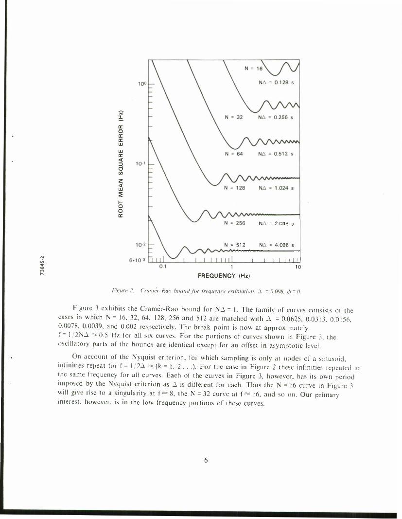
The following figure exhibits the Cramer-Rao bound behavior for frequencies much less than the Nyquist frequency. The Cramer-Rao bound (B22)1 2 computed from (8) is plotted in Figure 2. taking N = 16, 32, 64, 128, 256 and 512 successive samples separated in time by a constant interval of A = 0.008 s. It is immediately obvious that the Cramer-Rao bound decreases when N, the number of samples taken, increases. The break point between the monotonic and oscillatory parts of each curve occurs at f= I 2NA which is at increasingly lower frequency as N becomes greater. The third trend is that the Cramer-Rao bound decays to an asymptotic level as frequency increases. VSNR has been taken to be I here, however, it is implicit from Equations (8) for B22

that the Cramer-Rao bound shown in Figures 1 and 2 should be divided by vSNR in the more general case.

3 ID

tr O tr cc UJ

UJ cc <

a

o o cc

NA = 2.048 s

N = 512 NA = 4096 s >^»^»*—!».»,.»., .. . I i

J I I I 1 I 10

FREQUENCY (Hz)

Figure 2. Cramer-Rao bound for frequency estimation. S =0.008. 4> = 0.

Figure 3 exhibits the Cramer-Rao bound for NA= 1. The family of curves consists of the cases in which N = 16, 32, 64, 128, 256 and 512 are matched with A = 0.0625, 0.0313, 0.0156, 0.0078, 0.0039, and 0.002 respectively. The break point is now at approximately 1 = 1 /2NA =* 0.5 Hz for all six curves. For the portions of curves shown in Figure 3, the oscillatory parts of the bounds are identical except for an offset in asymptotic level.

On account of the Nyquist criterion, for which sampling is only at nodes of a sinusoid, infinities repeat for f = 1 2A « (k = 1, 2 . . .). For the case in Figure 2 these infinities repeated at the same frequency for all curves. Each of the curves in Figure 3, however, has its own period imposed by the Nyquist criterion as A is different for each. Thus the N = 16 curve in Figure 3 will give rise to a singularity at f = 8, the N = 32 curve at f«* 16, and so on. Our primary interest, however, is in the low frequency portions of these curves.

cr O cr cr LU

UJ cr <

a

< UJ

o cr

m 10 ' 10°

FREQUENCY (Hz)

Figure 3. Cramer-Rao hound for frequency estimation. 4> - ft AN = /.

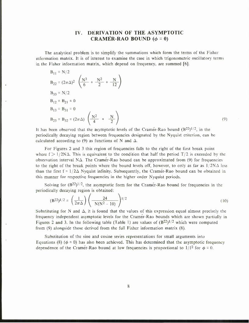
IV. DERIVATION OF THE ASYMPTOTIC CRAMER-RAO BOUND (<t> = 0)

The analytical problem is to simplify the summations which form the terms of the Fisher information matrix. It is of interest to examine the case in which trigonometric oscillatory terms in the Fisher information matrix, which depend on frequency, are summed [6]:

B33 = N/2

B,2 = B2| = 0

(9)

It has been observed that the asymptotic levels of the Cramer-Rao bound (B22)'/2, in the periodically decaying region between frequencies designated by the Nyquist criterion, can be calculated according to (9) as functions of N and A.

For Figures 2 and 3 this region of frequencies falls to the right of the first break point where f > 1/2NA. This is equivalent to the condition that half the period T/2 is exceeded by the observation interval NA. The Cramer-Rao bound can be approximated from (9) for frequencies to the right of the break points where the bound levels off, however, to only as far as 1/2NA less than the first f = 1/2A Nyquist infinity. Subsequently, the Cramer-Rao bound can be obtained in this manner for respective frequencies in the higher order Nyquist periods.

Solving for (B22)'/2, the asymptotic form for the Cramer-Rao bound for frequencies in the periodically decaying region is obtained:

Substituting for N and A, it is found that the values of this expression equal almost precisely the frequency independent asymptotic levels for the Cramer-Rao bounds which are shown partially in Figures 2 and 3. In the following table (Table I) are values of (B22)'/2 which were computed from (9) alongside those derived from the full Fisher information matrix (8).

Substitution of the sine and cosine series representations for small arguments into Equations (8) {<$> - 0) has also been achieved. This has determined that the asymptotic frequency dependence of the Cramer-Rao bound at low frequencies is proportional to 1/f2 for <f> - 0.

TABLE 1

Calculated Asymptotic Cramer -Rao Bound

N A (B22}1/2

from (9) from (10)

16 0.008 1.61 1.55

32 0.008 0.55 0.54

64 0.008 0.19 0.19

128 0.008 0.068 0.068

256 0.008 0.024 0.024

512 0.008 0.008 0.008

16 0.0625 0.206 0.199

32 0.0313 0.141 0.138

64 0.0156 0.099 0.098

128 0.0078 0.070 0.069

256 0.0039 0.049 0.049

512 0.002 0.034 0.034

V. NUMERICAL RESULTS FOR NON-ZERO PHASE

Figure 4 depicts the Cramer-Rao bound as a function of frequency when 0 = 0, n-/4, n/2 and 37T/4 for the case in which N = 64 and A = 0.008. The bound was computed from the full Fisher information matrix (8). It can be discerned that the oscillations decay so that asympotically the curves all approach a single Cramer-Rao bound level equal to that for 0 = 0, N = 64, A = 0.008 (Figure 2). The frequency dependence of the bound at low frequencies, for 0 = 77-/2, is determined to be 1/f. For frequencies less tha 0.2 Hz, the asymptotic behavior of the Cramer-Rao bounds for 0 - 0 and 0 = 7r/2 form an envelope about all of the phases shown in Figure 4.

Figure 5 departs from Figure 3 by only a small amount for f > 1. Figure 3 was obtained with 0 = 0. The former is created by taking the Cramer-Rao bound [computed from Equations (8)] with the phase which yields the highest Crame'r-Rao bound out of 100 phases

in t ID CO

10' MM 1 1 1 I 1 1 1 1 1 l 1 1

\ <|> : 0 - _

I * = 37TV4 - oc o DC DC UJ

-

SQ

UA

RE

o o -

\ <t> = 7T/2

-

Z < UJ

5 _

1- o o oc

. 't> = 7T/4

10' i I i I 1 1 1 1 1 I 1 III i I I

5-102 10' 10°

FREQUENCY (Hz)

Figure 4. Cramer- Rao bound for frequency estimation. N = 64, A = 0.008.

10

equally spaced between 0 and n. The behavior of the Cramer-Rao bound for worst case phase has already been shown in [2], however, this is for the case of a constant sampling interval A

and large frequency.

NA is constrained to be equal to 1 for both Figures 3 and 5. The break point between the monotonic and periodic segments in the family of curves in Figure 5 occurs at approximately f = l/NA, while for Figure 3 is at approximately 1/2NA. The lower break point for the case of </> = 0 is equal to the first null in sin Nw/sin w, where w = 7r/N, and w = 27rfA, which is exactly

f= I/2NA.

or O <r oc

DC < o C/3

< LU

I- o o DC

in in

102 10 ' 10«

FREQUENCY (Hz)

Figure 5. Cramer-Rao bound for frequency estimation. Worst case <t>. -VV- /.

II

VI. NORMALIZATION OF THE CRAMER-RAO BOUND: TRADE-OFFS INVOLVING NA AND SNR

One conclusion which can be drawn from Figures 2 and 3 in the previous section is that the width of the main lobe of the Cramer-Rao bound curves is the parameter I/2NA. This can be identified with the resolution of the estimation process. The greater the observation interval NA, the smaller will be the resolution <5f = 1/2NA. This trend can be likened to that of a square wave and its Fourier transform. The wider the square wave is, the smaller the width to the first null of its Fourier transform will be.

In Figure 6, the Cramer-Rao bound af normalized by the resolution Sf = 1/2NA is plotted against the frequency normalized by Sf. This is achieved for N = 16, 32, 64, 128, 256, and 512, for A = 0.008 in each case. These are the same parameters as were used for the unnormalized case in Figure 2. The curves of the family which results all break at the same f/Sf and are separated by a constant multiple for all f/Sf.

s

in

<o

10 i -

f/5f

Figure 6. Normalized Cramer-Rao bound for frequency estimation. <t> = 0

12

It was shown in Equation (10) of Section IV that the asymptotic Crame'r-Rao bound is on the order of 1/N3/2A. Thus the normalized Cramer-Rao bound of/Sf is on the order of l/\/N. Another piece of information we can extract from scaling the Cramer-Rao bound is that the family of curves in Figure 6 can be collapsed to one of \/N af/6f versus f/5f. This is shown in Figure 7 where for numerical convenience another scaling factor y/l/64 has been included. The family of curves is thus represented by the single relationship of vN/64 Of/Sf versus f/Sf.

From Figure 7 it can be observed that, in the low frequency region where f< 1/2NA, the slope of the curve is approximately -2, for 0 = 0.

101

J i i i i i 11 _i i i i i i 11

100

f/6f 10

Figure 7. Fully normalized Cramer-Rao bound.

Pf C <5f = / fv2 Thus \/N/64 -, or af *=*

(M N7/2A3f2 (ID

where 8i = rrr— and C «« 0.1 2NA

13

This relation represents the dependence of the Cramer-Rao bound on frequency, for low frequencies mapped onto the limb of the curve which lies to the left of the break point.

The following examples are designed to exemplify the trade-offs of NA and SNR which can be determined using Figure 7.

Example 1: Given f = 2 Hz, Sf = 1 Hz, and SNR = 1, what are N and A such that the Cramer-Rao bound Of equals 0.1?

For f/<5f= 2, it is shown in Figure 8 that vN/64 of/5f equals approximately 0.2. Since a(ld{ = 0.1, N can be solved for and is found to be 256. It is also known that 5f = 1/2NA = 1 Hz, so with N = 256, A need be no larger than 0.002.

10'

*

z

10°

03

02

101

0032

J

1 1

1

1 1 1 1 1 1

1 1

1 1 1

»fl

1 111

1 1 1

1 I

1 1

1 1

1

SNR « 100 j

- 1 1 I I ill i i 1 i i I I l 1 1 1 0 64 10°

f/5f 200 10

Figure 8. Fully normalized Cramer-Rao bound (example I. 2).

For the second example, SNR is for the first time a variable parameter and is no longer set equal to 1. It can be discerned from Equation set (8) that (B22)'/2, the Cramer-Rao bound, will be proportional to l/A/oR or 1/vSNR.

14

Example 2: Using Figure 7, the problem here is to determine what SNR ratio is necessary so that af = 0.2 Hz when f = 2 Hz, N = 16, and A = 0.01.

It is known that 5f = 1/2NA = 1/0.32 Hz so that f/5f = 0.64. The design point for which VSNR will be determined is, for N= 16, at \/l6/64 af/5f. When af= 0.2 Hz and 5f = 1/0.32 Hz, this point falls at 0.032 on the vertical axis of Figure 8. However, the actual point on the axis to which f/6f = 0.64 corresponds is approximately 0.3. Therefore a VSNR ratio of *" 10 is required to reduce the normalized and scaled value of the Cramer-Rao bound from "* 0.3 to 0.032.

15

VII. SUMMARY AND CONCLUSIONS

The influences of number of samples, sampling frequency, phase, and signal-to-noise ratio on the Cramer-Rao bound for frequency estimation of sine waves in Gaussian white noise have been studied. A closed form expression for the asymptotic Cramer-Rao bound has been derived which exhibits a 1/N3/2A dependence. The Cramer-Rao bound normalized by the resolution and scaled by vN, where N is the number of samples, reduces the family of curves parameterized by N and A to a single operating curve. Examples of trade-offs involving NA and SNR ratio are determined by this composite relationship among the parameters.

As long as the measurement interval NA is at least a half cycle of the sine wave, the Cramer-Rao bound is close to being independent of frequency; however, in the instance of worst case phase the measurement interval must cover an entire cycle. In the low frequency region where NA is less than half a cycle, the bound on Of varies as 1/f2 for phase 0 = 0, and 1/f for phase <j> = 77-/2. For example, if the frequency is 0.1 Hz, the value of af will be at most 25 times larger than for a frequency of 0.5 Hz, with the same parameters N, A. If the signal-to-noise is sufficiently high, it is still possible to obtain accurate frequency estimates even in this low frequency region.

16

ACKNOWLEDGMENTS

I wish to thank Dr. Keh-Ping Dunn, Dr. Daniel O'Connor, and Dr. Stephen Weiner for their help and suggestions in preparing this paper. The programming assistance of Mr. Paul Warren is gratefully acknowledged. I also wish to express my appreciation to Miss Nancy Asadoorian and Miss Laura Parr for their typing expertise.

REFERENCES

1. D.C. Rife and R.R. Boorstyn, "Single-tone Parameter Estimation from Discrete- Time Observations," IEEE Trans. Inf. Theory IT-20 (September 1974).

2. D.C. Rife and R.R. Boorstyn, "Multiple Tone Parameter Estimation from Discrete- Time Observations," Bell Syst. Tech. J. 55 (November 1976).

3. M.J. Tsai, "The ML Method for Frequency Estimation of Real Sinusoids in Noise," Technical Report 689, Lincoln Laboratory, MIT (27 July 1984), DTIC AD-A146053.

4. H.L. Van Trees, Detection, Estimation, and Modulation Theory Part 1 (Wiley, New York, 1968).

5. D. Slepian, "Estimation of Signal Parameters in the Presence of Noise," IRE Trans. Inf. Theory PGIT-3 (March 1954).

6. L.B.W. Jolley, Summation of Series (Dover, New York, 1961).

17

UNCLASSIFIED SECURITY CLASSIFICATION OF THIS PAGE (When Data Entered)

REPORT DOCUMENTATION PAGE READ INSTRUCTIONS BEFORE COMPLETING FORM

1. REPORT NUMBER

ESD-TR-85-323

2. GOVT ACCESSION NO 3. RECIPIENT'S CATALOG NUMBER

4. TITLE (and Subtitle)

Cramer-Rao Bound Analysis for Frequency Estimation of Sinusoids in Noise

I. TYPE OF REPORT ft PERIOD COVERED

Technical Report

6. PERFORMING ORG. REPORT NUMBER

Technical Report 727

7. AUTHOR^

Joy M. Skon

8. CONTRACT OR GRANT NUMBERS

F19628-85-C-0002

9 PERFORMING ORGANIZATION NAME AND ADDRESS

Lincoln Laboratory, MIT P.O. Box 73 Lexington, MA 02173-0073

10. PROGRAM ELEMENT. PROJECT. TASK AREA & WORK UNIT NUMBERS

Program Element Nos. 63220C and 63304A

II. CONTROLLING OFFICE NAME AND ADDRESS

U.S. Army Strategic Defense Command Sensors Directorate P.O. Box 1500 Huntsville, AL 35807-3801

Huntsville 12. REPORT DATE

24 March 1986

13, NUMBER OF PAGES

22 14. MONITORING AGENCY NAME & ADDRESS (if different from Controlling Office)

Electronic Systems Division Hanscom AFB, MA 01731

IS. SECURITY CLASS, (of this Report)

Unclassified

15.i. DECLASSIFICATION DOWNGRADING SCHEDULE

16 DISTRIBUTION STATEMENT (of thu Report)

Approved for public release; distribution unlimited.

17 DISTRIBUTION STATEMENT (of the abstract entered in Block 20, if different from Report)

18 SUPPLEMENTARY NOTES

None

19. KEY WORDS (Continue on reverse side if necessary and identify by block number)

Cramer-Rao bound frequency estimation sampling frequency

signal-to-noise ratio resolution sinusoids

20. ABSTRACT (Continue on reverse side if necessary and identify by block number)

The Cramer-Rao inequality is used to determine a lower bound on the variance with which a sinusoidal frequency can be estimated in the presence of Gaussian white noise. A parametric study has elucidated the influence of number of samples (N), sampling frequency (1/A), phase (<£), and signal-to- noise ratio (SNR) on the Cramer-Rao bound. A closed form expression for the asymptotic level to which the Cramer-Rao bound decays is characterized and, for low frequencies, the bound is determined analytically and graphically. The form of the Cramer-Rao bound is linked to resolution in the sampling problem. Identification of trade-offs characterizing the sensitivity of the bound and parameters associated with it are discussed.

DD FORM

1 Jin 73 1473 EDITION OF 1 N0V 65 IS OBSOLETE UNCLASSIFIED

SECURITY CLASSIFICATION OF THIS PAGE (When Data Knlerrdl