covariant symanzik identities
TRANSCRIPT

PROBABILITY andMATHEMATICAL
PHYSICS
msp
COVARIANT SYMANZIK IDENTITIES
ADRIEN KASSEL AND THIERRY LÉVY
2:32021

msp
PROBABILITY andMATHEMATICAL
PHYSICSVol. 2, No. 3, 2021
https://doi.org/10.2140/pmp.2021.2.419
COVARIANT SYMANZIK IDENTITIES
ADRIEN KASSEL AND THIERRY LÉVY
Classical isomorphism theorems due to Dynkin, Eisenbaum, Le Jan, and Sznitman establish equalitiesbetween the correlation functions or distributions of occupation times of random paths or ensembles ofpaths and Markovian fields, such as the discrete Gaussian free field. We extend these results to the case ofreal, complex, or quaternionic vector bundles of arbitrary rank over graphs endowed with a connection, byproviding distributional identities between functionals of the Gaussian free vector field and holonomies ofrandom paths. As an application, we give a formula for computing moments of a large class of random, ingeneral non-Gaussian, fields in terms of holonomies of random paths with respect to an annealed randomgauge field, in the spirit of Symanzik’s foundational work on the subject.
Introduction 4191. Graphs, paths, and loops 4252. Vector bundles 4343. A covariant Feynman–Kac formula 4454. The Gaussian free vector field 4495. Isomorphism theorems of Dynkin and Eisenbaum 4526. Isomorphism theorems of Le Jan and Sznitman 4587. Symanzik identity 469Concluding remarks 472Acknowledgements 473References 473
Introduction
Following the pioneering work of Symanzik [1969] where he established, for the needs of Euclideanquantum field theory, a heuristic correspondence between random fields and random paths, Dynkin [1980]initiated the mathematical study of the deep relations that exist between a Markovian field and a Markovprocess when they share the same generator. Another seminal contribution in this direction was madearound the same time by Brydges, Fröhlich and Spencer [Brydges et al. 1982].
The joint study of random fields over a space and random paths in the same space may be seen as aprobabilistic instance of the general principle that the geometry of a space can be understood by lookingat good functions that live on it as well as by looking at its points.
MSC2020: 60J55, 60J57, 81T25, 82B20.Keywords: discrete potential theory, Laplacian on vector bundles, Gaussian free vector field, random walks, covariant
Feynman–Kac formula, Poissonian ensembles of Markovian loops, local times, isomorphism theorems, discrete gauge theory,holonomy.
419

420 ADRIEN KASSEL AND THIERRY LÉVY
The essence of the situation that gives rise to the correspondence investigated by Symanzik, Dynkin andmany others after them, is the existence, on a topological or geometrical space, of a differential operator(say a Laplacian) which determines on one hand a random field on the space (the Gaussian free field)and on the other hand a random motion within the space (the Brownian motion). Both random objectsexpress something of the geometry of the underlying space, and the general problem is to understandhow the properties of the one mirror the properties of the other.
A fairly general framework where a Laplacian operator is defined is that of a Riemannian manifold. Anatural extension of this framework is that of a Euclidean or Hermitian vector bundle over a Riemannianmanifold, endowed with a connection. In this case, the Laplacian acts on sections of the vector bundle,and the role of the random field will be played by a random vector field.
The goal of this paper is to investigate some of the relations between random vector fields and randompaths in a discrete version of the setting that we just described, namely on a vector bundle with a connectionover a finite graph. There, the discrete nature of space keeps the analysis simple, making for instance anyprocedure of renormalisation irrelevant, but the presence of the vector bundle lets interesting geometryenter the picture. In this framework, we will give appropriate formulations and complete self-containedproofs of the natural analogues of four classical theorems, sometimes called “isomorphism theorems”,due to Dynkin, Eisenbaum, Le Jan, and Sznitman, and of a fifth result in the original spirit of Symanzik.We insist that these classical statements are not used in our proofs, and that the proofs that we proposealso provide a geometrical insight into these classical statements. In their original form, these theoremsrelate occupation times of various random paths and functions of the square of the Gaussian free field.An interesting feature of the extensions of these results that we propose is the prominent role playednot only by random paths on the graph, but also by the parallel transport determined along them by theconnection.
Let us illustrate, without too much formal preparation, and on the example of an identity that isfundamental to our study, the role played by the parallel transport. Suppose x and y are vertices of ourgraph. Let Px denote the distribution of the natural continuous time random walk issued from x . Let tbe a positive real. If γ is a path in the graph, we denote by γt its position at time t , and by hol(γ|[0,t))
the holonomy, or parallel transport, along the restriction to [0, t) of γ . If γt = y, and provided t is not ajump time of γ , this is a linear isometry from the fibre over y to the fibre over x . Then, in a matricialexpression of the operator e−t1 acting on the space of vector fields over the graph, that is, on the directsum of all the fibres of the bundle, the block corresponding to a linear map from the fibre over y to thefibre over x can be expressed as
(e−t1)x,y =
∫hol(γ|[0,t))
−11{γt=y} dPx(γ ). (1)
This equation is indeed the simplest case of a (covariant) Feynman–Kac formula that will be oneof our main tools in proving our five main results. In the case where the bundle is a line bundleand the connection is trivial, this formula is an equality of scalars, saying nothing more than thefact that the Laplacian is the infinitesimal generator of the semigroup of the random walk on thegraph.

COVARIANT SYMANZIK IDENTITIES 421
x ye
Fx ' Rr Fy ' Rr
he
h−1e
Figure 1. A discrete real vector bundle F of rank r over a graph with an orthogonal connection h.
Overview of the results. In order to give a more precise idea of at least some of these results, it isnecessary to be a little more specific about our framework. We consider a real, complex or quaternionicvector bundle of arbitrary rank over a finite graph endowed with a unitary connection. In this introduction,for the sake of simplicity, we will focus on the real case. The connection, in this case, consists in anorthogonal matrix over each oriented edge of the graph, called the holonomy along this edge. Theholonomies along an edge and the same edge with the opposite orientation are inverses of each other (seeFigure 1). We denote the connection by h. The holonomy hol(γ ) along a path γ is the ordered product ofthe holonomies along the edges traversed by the path. It is an isometry from the fibre over the startingpoint of the path to the fibre over its finishing point.
The connection h gives rise to a quadratic form
E( f )= 12
∑e=xy
‖ fx − h−1e fy‖
2
on the space of vector fields over the graph, the sum being extended to all oriented edges of the graph.To this quadratic form is associated a centred Gaussian random vector field 8, called the Gaussian freevector field (see Figure 2 for an illustration and Section 2L for a precise definition). Let us stress thatexcept for very specific choices of the connection, there do not exist bases of the fibres in which thecomponents of the field would be independent Gaussian free fields.
The covariance of the Gaussian free vector field has an expression in terms of random walk. Indeed,if x and y are vertices, and if ξ and η are respectively vectors of the fibres over x and y, then
E[〈ξ,8x 〉〈8y, η〉] =
∫〈ξ, hol(γ )−1(η)〉 dνx,y(γ ), (2)
where νx,y is a finite measure on the set of paths from x to y (see Definition 1.10).By virtue of Wick’s formula, one can turn (2) into an expression for the moments of the field 8, that
is, for quantities of the form E[( f1,8) · · · ( fk,8)], where f1, . . . , fk are vector fields. This expression isan integral of products of matrix coefficients of holonomies along paths with respect to a multibridgemeasure.
422 ADRIEN KASSEL AND THIERRY LÉVY
All the results presented in this paper will follow more or less directly from identities slightly moregeneral than, but similar to (2). For instance, a special case of our analogue of Dynkin’s theorem(Theorem 5.1) goes as follows. We denote by `z(γ ) the time spent by a path γ at a vertex z.
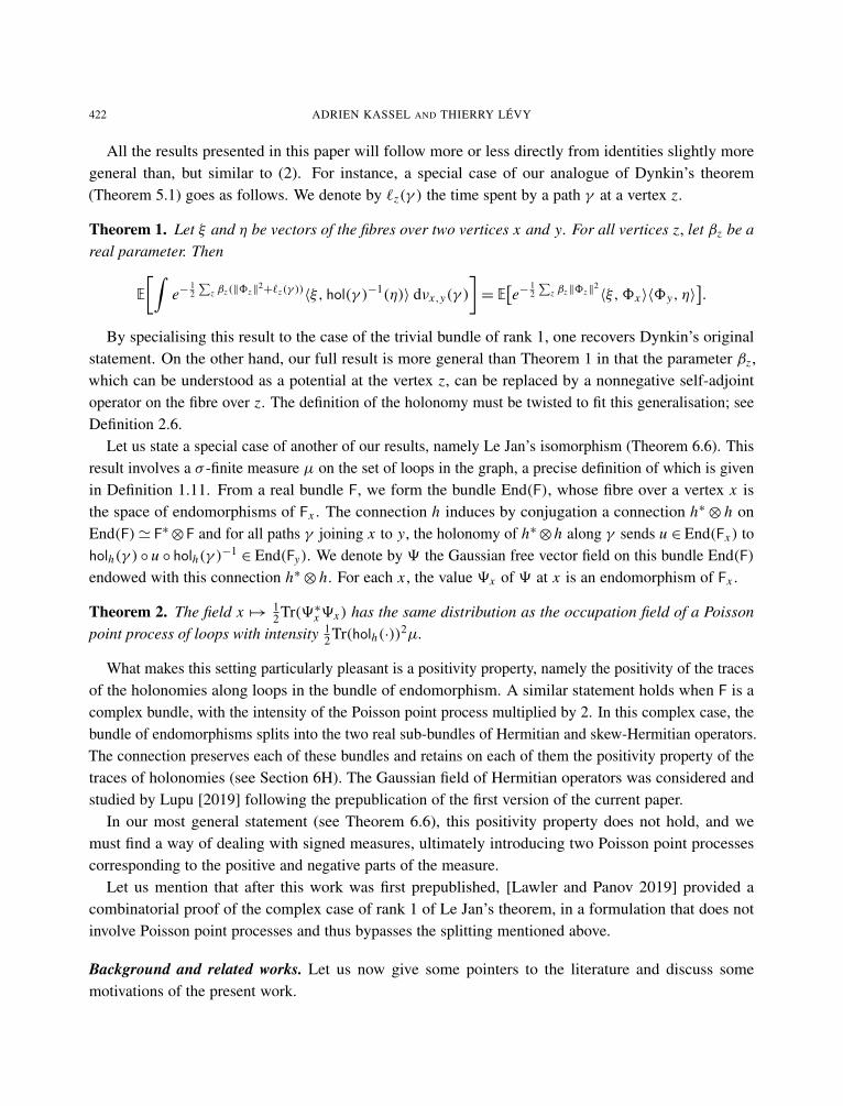
Theorem 1. Let ξ and η be vectors of the fibres over two vertices x and y. For all vertices z, let βz be areal parameter. Then
E
[∫e−
12∑
z βz(‖8z‖2+`z(γ ))〈ξ, hol(γ )−1(η)〉 dνx,y(γ )
]= E
[e−
12∑
z βz‖8z‖2〈ξ,8x 〉〈8y, η〉
].
By specialising this result to the case of the trivial bundle of rank 1, one recovers Dynkin’s originalstatement. On the other hand, our full result is more general than Theorem 1 in that the parameter βz ,which can be understood as a potential at the vertex z, can be replaced by a nonnegative self-adjointoperator on the fibre over z. The definition of the holonomy must be twisted to fit this generalisation; seeDefinition 2.6.
Let us state a special case of another of our results, namely Le Jan’s isomorphism (Theorem 6.6). Thisresult involves a σ -finite measure µ on the set of loops in the graph, a precise definition of which is givenin Definition 1.11. From a real bundle F, we form the bundle End(F), whose fibre over a vertex x isthe space of endomorphisms of Fx . The connection h induces by conjugation a connection h∗⊗ h onEnd(F)' F∗⊗F and for all paths γ joining x to y, the holonomy of h∗⊗h along γ sends u ∈ End(Fx) toholh(γ ) ◦ u ◦ holh(γ )−1
∈ End(Fy). We denote by 9 the Gaussian free vector field on this bundle End(F)endowed with this connection h∗⊗ h. For each x , the value 9x of 9 at x is an endomorphism of Fx .
Theorem 2. The field x 7→ 12 Tr(9∗x9x) has the same distribution as the occupation field of a Poisson
point process of loops with intensity 12 Tr(holh(·))2µ.
What makes this setting particularly pleasant is a positivity property, namely the positivity of the tracesof the holonomies along loops in the bundle of endomorphism. A similar statement holds when F is acomplex bundle, with the intensity of the Poisson point process multiplied by 2. In this complex case, thebundle of endomorphisms splits into the two real sub-bundles of Hermitian and skew-Hermitian operators.The connection preserves each of these bundles and retains on each of them the positivity property of thetraces of holonomies (see Section 6H). The Gaussian field of Hermitian operators was considered andstudied by Lupu [2019] following the prepublication of the first version of the current paper.
In our most general statement (see Theorem 6.6), this positivity property does not hold, and wemust find a way of dealing with signed measures, ultimately introducing two Poisson point processescorresponding to the positive and negative parts of the measure.
Let us mention that after this work was first prepublished, [Lawler and Panov 2019] provided acombinatorial proof of the complex case of rank 1 of Le Jan’s theorem, in a formulation that does notinvolve Poisson point processes and thus bypasses the splitting mentioned above.
Background and related works. Let us now give some pointers to the literature and discuss somemotivations of the present work.
COVARIANT SYMANZIK IDENTITIES 423
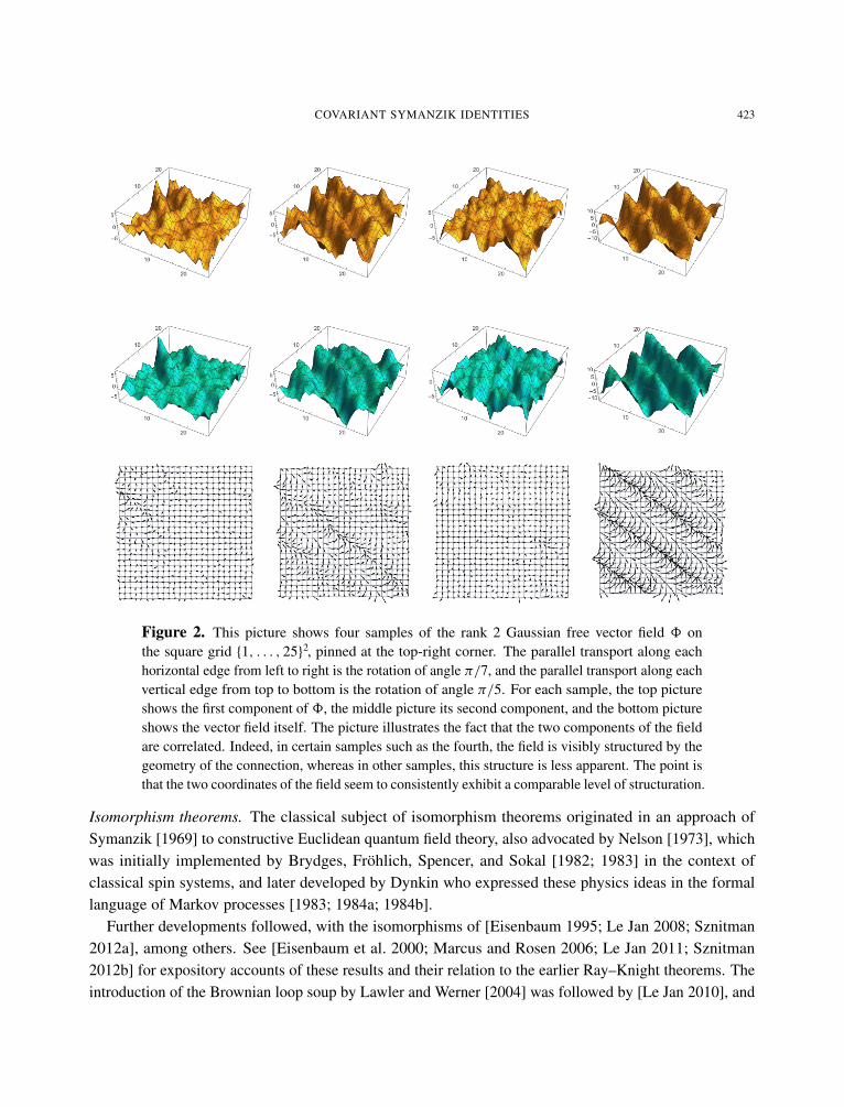
Figure 2. This picture shows four samples of the rank 2 Gaussian free vector field 8 onthe square grid {1, . . . , 25}2, pinned at the top-right corner. The parallel transport along eachhorizontal edge from left to right is the rotation of angle π/7, and the parallel transport along eachvertical edge from top to bottom is the rotation of angle π/5. For each sample, the top pictureshows the first component of 8, the middle picture its second component, and the bottom pictureshows the vector field itself. The picture illustrates the fact that the two components of the fieldare correlated. Indeed, in certain samples such as the fourth, the field is visibly structured by thegeometry of the connection, whereas in other samples, this structure is less apparent. The point isthat the two coordinates of the field seem to consistently exhibit a comparable level of structuration.
Isomorphism theorems. The classical subject of isomorphism theorems originated in an approach ofSymanzik [1969] to constructive Euclidean quantum field theory, also advocated by Nelson [1973], whichwas initially implemented by Brydges, Fröhlich, Spencer, and Sokal [1982; 1983] in the context ofclassical spin systems, and later developed by Dynkin who expressed these physics ideas in the formallanguage of Markov processes [1983; 1984a; 1984b].
Further developments followed, with the isomorphisms of [Eisenbaum 1995; Le Jan 2008; Sznitman2012a], among others. See [Eisenbaum et al. 2000; Marcus and Rosen 2006; Le Jan 2011; Sznitman2012b] for expository accounts of these results and their relation to the earlier Ray–Knight theorems. Theintroduction of the Brownian loop soup by Lawler and Werner [2004] was followed by [Le Jan 2010], and

424 ADRIEN KASSEL AND THIERRY LÉVY
an isomorphism for Brownian interlacement was given by Sznitman [2013]. The whole subject has seenfurther recent developments, attested among many other papers by [Lupu 2016; Werner 2016; Qian andWerner 2019; Lupu and Werner 2016; Zhai 2018; Ding and Li 2018; Sabot and Tarres 2016; Sznitman2016; Abächerli and Sznitman 2018; Drewitz et al. 2018].
Very recently, in [Bauerschmidt et al. 2021], the authors considered other geometries for the targetspace of the Gaussian field than the Euclidean one, namely spherical and hyperbolic geometries. Theyprovide a unified exposition of three Dynkin isomorphism theorems relating fields to not necessarilyMarkovian random paths, namely the simple, vertex-reinforced, and vertex-diminished random walks.
Lattice gauge theories. The geometric framework of connections on graphs is the classical framework oflattice gauge theory, which gives a finite approximation scheme to continuous gauge theories, such as theYang–Mills theory; see [Lévy 2020] for a recent survey of progress on Yang–Mills theory in dimension 2.One long-term general motivation for our study is the construction of a tractable probabilistic model forthe interaction of a gauge field with a fermionic field, that is, for a random connection coupled to a modelof statistical physics. The Gaussian free vector fields and the loop soups appearing in this paper wouldrather qualify as bosonic, but there are hints that they are related to the fermionic side. For instance, oneway to describe Le Jan’s loop measure is by means of Wilson’s algorithm for sampling a uniform spanningtree by erasing loops from random walk trajectories ([Le Jan 2011; Lawler 2018]). The distribution of theensemble of erased loops is related to Le Jan’s measure, and the uniform spanning tree, of determinantalnature, could qualify as fermionic matter.
In a work in preparation [Kassel and Lévy ≥ 2021] we introduce an analogue of uniform spanning treemeasures in the context of vector bundles over graphs and discuss links to electrical networks and randomwalk holonomies. A preview of the definition of these quantum spanning forests is available in [Kasseland Levy 2019, Section 1.5]. Spanning forests on vector bundles of real, complex, or quaternionic rank 1were investigated by Kenyon [2011] (see also [Kassel and Kenyon 2017]), and the slightly different butrelated case of loop soups on graph coverings was considered in [Le Jan 2017].
In the work of physicists, it is customary that computations involving matrix models, connections, andgauge symmetry, can be expressed in terms of random surfaces or topological expansions. In the presentpaper, we are dealing with random paths rather than surfaces. Nevertheless, in the framework consideredby Lupu [2019] and described before Theorem 2, topological expansions over maps do appear. Anotherway in which such higher-dimensional expansions arise is by considering Gaussian random forms onthe cells of a simplicial complex and relating them to simplicial random walks [Kassel and Rosenthal2016]. A combinatorial relationship between vector bundles over graphs and simplicial complexes ofhigher dimension was also suggested in [Kassel and Lévy 2020, Section 7.1].
Finally, the relationship between fields and paths that we explore fits nicely in the framework of gaugetheory: when the law of the Markovian field is gauge invariant (as for instance in Theorem 2), we expressit in terms of a random process determined by traces of holonomies along loops. These traces (the averagesof which with respect to a random connection are called Wilson loops) are indeed gauge invariant, andknown, in many cases of interest, to generate a dense subalgebra of gauge-invariant functions; see, e.g.,[Lévy 2004].

COVARIANT SYMANZIK IDENTITIES 425
Covariant Feynman–Kac formula. One of the most useful results for our study is a covariant versionof the Feynman–Kac formula. This formula can be thought of as a discrete analogue of a continuumversion which can be traced back at least to the work of Norris [1992] (see also [Albeverio et al. 1989]) instochastic differential geometry, and which can also be found, in a different guise for discrete time walks,in earlier works of Brydges, Fröhlich, and Seiler [1979] on lattice gauge theories as we discovered aftercompleting our work. Batu Güneysu also kindly informed us of related work in [Güneysu et al. 2014].
Organisation of the paper. Sections 1 and 2 are devoted to a detailed description of the basic setup ofvector bundles over graphs which we use throughout. The main novelty consists in the introduction, inSection 2, of a notion of twisted holonomy (Definition 2.6) which, we believe, is a fruitful extension inour geometric framework of classical exponential functionals of local times. In Section 3, we prove thecovariant Feynman–Kac formula (Theorem 3.1).
The main results of the paper are presented in Sections 5, 6, and 7. Section 5 presents a very generalformulation of both Dynkin’s (Theorem 5.1) and Eisenbaum’s (Theorem 5.2) isomorphism theorems.Our formulation is targeted at giving more insight into the relation between these isomorphism theoremsand the probabilistic formulation of potential theory; see, for instance, (46). We believe that a part of themeaning of these isomorphisms appears more clearly in our general framework than in the classical case.In any case, the relations that we prove between twisted holonomies and fields extend the known relationsbetween random paths and Gaussian fields, since the class of functionals obtained from twisted holonomiescaptures more faithfully, thanks to the noncommutativity of the gauge groups, the actual geometry ofpaths, whereas local times ignore much of the chronological unfolding of events in a trajectory.
Section 6 presents a unified formulation (Theorem 6.6) of the isomorphisms of Le Jan and Sznitmanin the context of vector bundles. The most general statement is rather involved, with notions such assplittings, colour decompositions, signed measures, and amplitudes, all introduced gradually. We alsopresent a special case of the statement (Theorem 6.7) which is much more concise and holds for certaintype of connections which we call trace-positive.
Finally, Section 7 builds on the previous sections to prove a statement (Theorem 7.3) relating momentsof a large class of random sections to holonomies of random paths under an annealed gauge field. Wecall these formulas covariant Symanzik identities.
1. Graphs, paths, and loops
1A. Graphs. In this first section, we give a precise definition of the graphs that we will consider through-out this paper. One aspect in which this definition differs from that used for example in [Sznitman 2012b]or [Le Jan 2011] is that we allow more than one edge between two vertices of a graph. We also allowloop edges, that is, edges with identical end points.
Definition 1.1. A graph is a quintuple G= (V,E, s, t, i) consisting of• two nonempty finite sets V and E,• two maps s, t : E→ V, and• a fixed-point free involution i of E such that t ◦ i = s holds.

426 ADRIEN KASSEL AND THIERRY LÉVY
Figure 3. The graph depicted on the left has 6 vertices and 12 geometric edges. The picture onthe right shows the 24 edges of this graph.
The elements of V are the vertices of the graph, the elements of E its edges. Each edge e is orientedand joins its source s(e) to its target t (e).
The involution i induces an equivalence relation on E and the equivalence classes of these relations,that is, the pairs {e, i(e)}, are called the geometric edges of the graph. The set of geometric edges of thegraph is denoted by [E].
We will often write e = s(e), e = t (e) and e−1= i(e) for the source, target, and inverse of an edge.
We will also write a graph simply as a pair (V,E) and not mention the maps s, t, i .We say that the graph G= (V,E) is connected if for all x, y ∈ V, there exists a well-chained alternating
sequence (x0, e1, x1, . . . , en, xn) of vertices and edges such that x0= x , xn = y and for all k ∈ {1, . . . , n},the edge ek starts at xk−1 and finishes at xk . In this paper, we will only work with connected graphs.
Definition 1.2. In a graph G= (V,E), we call well a proper nonempty subset W of the set V of vertices.The elements of V \W are called the proper vertices of the graph. The subset
∂(V \W)= {x ∈ V \W : there exists e ∈ E, s(e)= x and t (e) ∈W}
of V is called the rim of the well.
A typical situation giving rise to graphs with wells is that where an infinite graph is exhausted by anincreasing sequence V1 ⊂ V2 ⊂ · · · of finite subgraphs. Then, for each n ≥ 1, one can consider the graphwith vertex set Vn+1, with the edges inherited from the infinite ambient graph, and with well Vn+1 \Vn .See Figure 3 for an illustration.
1B. Weights and measures. We will gradually introduce a certain amount of structure on the graphs thatwe consider. We start with a weighting of the edges.
Definition 1.3. Let G = (V,E) be a graph. A conductance on G is a positive real-valued functionχ : E→ (0,+∞) such that χ ◦ i = χ .
We think of χ as a measure on the set of edges of the graph. We shall usually write χe instead of χ(e)for the conductance of an edge e. The pair (G, χ) is called a weighted graph.
Let G= (V,E) be a graph with a well endowed with a conductance χ . We define the reference measureon G as the function λ : V→ (0,+∞) defined by
for all x ∈ V, λx =∑
e∈E:e=x
χe. (3)
COVARIANT SYMANZIK IDENTITIES 427
Let us emphasise that λ takes a positive value at every vertex, even on the vertices of the well.The part of λ that is due to the conductances of edges joining a proper vertex to a vertex of the well
plays a special role. We define, for every proper vertex x ,
κx =∑
e∈E:e=x,e∈W
χe.
By definition, the support of the measure κ , that is, the set of vertices x such that κx > 0, is the rim of thewell.
In this paper, unless explicitly stated otherwise, by a weighted graph with a well, we will always meanthe data of the collection of objects (W ⊂ V,E, s, t, i, χ, λ, κ) as defined in this section, and with thisnotation. We will moreover always assume that the graph is connected, in the sense explained above.
Let us conclude this section with a few terminological remarks. Firstly, the reader may find that thereis an absence of distinction between measures and functions in our presentation, as we took advantage ofthe discrete nature of our framework to identify the measures χ, λ, κ with their densities with respect tothe counting measures on E and V. We adopted these identifications because they allow for a simpler andlighter notation, but we also believe that they hide to some extent the true nature of the objects whichone manipulates (and which would appear more clearly in a continuous setup). Therefore, we invite thereader to check periodically that our statements are consistent in this respect and that our formulas are, inthe physical sense, homogeneous.
Secondly, the objects that we are considering are very classical and receive several different namesin the literature. The main reason for introducing them with care is that when dealing with twistedholonomies, one has to be careful with the precise definition of paths (when there are multiple edges,and when there are edges leading to the well, which we also consider backwards). The vertex or set ofvertices that we call the well is sometimes called the sink, and sometimes also the cemetery, and theauthors who use the latter name call the quantity that we denote by κ the killing rate. We prefer to avoida morbid terminology, but respect the tradition and keep the notation κ .1 An electric analogy is also oftenused in this context, accounting for the name of the conductance. In this terminology, the well should bethought of as an electric ground. This may be the place to mention that, depending on the analogy whichone chooses, the conductance of an edge can be understood as the inverse of an electric resistance, theinverse of a length, or the section of a water pipe.
1C. Discrete paths. Paths in graphs will play a crucial role in this study. The reader will soon noticethat it is not only important for us to know which vertices a path visits, but also which edges it traverses,and because this is not the most widespread point of view, we give complete definitions of the objectsthat we consider. We will mainly study paths indexed by continuous time, but it is convenient to definepaths indexed by discrete time first.
Let us fix a graph G= (V,E).
1We do find wells and their rims more inspiring than sinks and cemeteries, following Neruda [1973]: Hay que sentarse a laorilla/del pozo de la sombra/y pescar luz caída/con paciencia; [We must sit on the rim/of the well of darkness/and fish for fallenlight/with patience].
428 ADRIEN KASSEL AND THIERRY LÉVY
Definition 1.4. Let n ≥ 0 be an integer. The set of discrete paths of length n in G is the set
DPn(G)={(x0, e1, x1, . . . , en, xn) ∈ V× (E×V)n : for all k ∈ {1, . . . , n}, ek = xk−1 and ek = xk
}. (4)
The set of discrete paths on G is the disjoint union
DP(G)=⋃n≥0
DPn(G). (5)
For example, a discrete path of length 0 is simply a vertex, and a discrete path of length 2 is awell-chained sequence (x0, e1, x1, e2, x2) of vertices and edges. The length of a path, sometimes calledits combinatorial length, is the number of edges traversed by this path. In this work, as the previousdefinition indicates, we will only consider finite discrete paths.
A discrete path of positive length k is of course completely characterised by the sequence of k edgeswhich it traverses. Nevertheless, despite the fact that edges will play for us a more important role than isusual (because the parallel transport along parallel edges will not be assumed to be equal), we will stillpay a lot of attention to the sequence of vertices visited by paths, and it is useful to keep explicit track ofthis information in their definition.
The initial and final vertex of a discrete path p = (x0, e1, . . . , xn) are respectively denoted by p = x0
and p = xn .
Definition 1.5. A discrete loop is a discrete path with identical initial and final vertices. The set ofdiscrete loops of length n is denoted by DLn(G) and the set of all discrete loops by
DL(G)=⋃n≥0
DLn(G).
Note that DL0(G)= DP0(G)= V.
1D. Continuous paths. A path indexed by continuous time is a discrete path which spends, at eachvertex that it visits, a certain positive amount of time. Here is the formal definition.
Definition 1.6. Let G= (V,E) be a graph. A continuous path in G is an element of the set
P(G)=⋃n≥0
(DPn(G)× (0,+∞)n × (0,+∞]).
A continuous loop in G is an element of the set
L(G)=⋃n≥0
(DLn(G)× (0,+∞)n × (0,+∞]).
If p= (x0, e1, . . . , xn) is a discrete path, τ0, . . . , τn−1 are positive reals and τn is an element of (0,+∞],then we will denote the continuous path (p, τ0, . . . , τn) by
γ = ((x0, τ0), e1, (x1, τ1), . . . , en, (xn, τn)).
This path is understood as the trajectory of a particle which starts from x0, spends time τ0 at x0, jumpsto x1 through the edge e1, spends time τ1 at x1, and so on. The path p is said to be the discrete path

COVARIANT SYMANZIK IDENTITIES 429
underlying the continuous path γ . Note that a continuous loop spends at least two intervals of time at itsstarting point, one at the beginning and the other at the end of its course.
The times τ0, . . . , τn are called the holding times of γ . The total lifetime of γ is
|γ | = τ0+ · · ·+ τn.
The proper lifetime of γ is the time at which γ first hits the well:
τ(γ )= τ0+ · · ·+ τm−1, where m = inf{l ≥ 0 : xl ∈W}. (6)
It is understood that if the starting point of γ belongs to the well, then τ(γ )= 0, and that if γ never hitsthe well, then τ(γ )= |γ |.
To the path γ , we associate a right-continuous function from [0, |γ |) to V, which we also denote by γ .It is defined as follows: for every t ∈ [0, |γ |), there is a unique k ∈ {0, . . . , n} such that τ0+· · ·+ τk−1 ≤
t < τ0+ · · ·+ τk , and we set γt = xk . If t ∈ [0, τ0), then k = 0 and γt = x0. Informally,
γt =
n∑k=0
xk1[τ0+···+τk−1,τ0+···+τk)(t).
For every t ∈ (0, |γ |), we define the restriction of the continuous path γ to [0, t) by setting
γ|[0,t) =((x0, τ0), e1, . . . , ek−1, (xk−1, τk−1), ek, (xk, t − (τ0+ · · ·+ τk−1))
),
where k is the same integer as before. Note that the right-continuous function from [0, t) to V associatedto the continuous path γ|[0,t) is equal to the restriction to [0, t) of the right-continuous function from[0, |γ |) to V associated to γ .
Finally, if the total lifetime of γ is finite, we define the time-reversal, or inverse of γ as the path
γ−1= ((xn, τn), e−1
n , (xn−1, τn−1), . . . , e−11 , (x0, τ0)).
The total lifetime of γ−1 is the same as that of γ , and the right-continuous function from [0, |γ |) to V
associated to γ−1 is defined byγ−1
t = lims↑|γ |−t
γs .
1E. Discrete time random walk. We will now describe the natural random walk on a weighted graphwith a well. It is a random continuous path on the graph, for which we will start off by describing theunderlying random discrete path.
There is nothing complicated about this random discrete path: from any vertex, it selects randomlyone of the outgoing edges, using the conductances as probability weights, then goes to the other end ofthe selected edge, and from there repeats this procedure, until it hits the well. The reason why we givesome detail about this random walk is that, because our graph can have several edges between two givenvertices, and because we want to keep track of which edge the random walk chose (because the paralleltransport of the connection along it will be specific to that edge), we are slightly outside the classicalframework of Markov chains on the vertex set of a graph. The random walk that we want to consider can

430 ADRIEN KASSEL AND THIERRY LÉVY
however easily be derived, as we will now explain, from a natural Markov chain on the set of half-edgesof the graph.
Let us consider a graph G= (V,E). We introduce the sets
Hs = {(x, e) ∈ V×E : x = s(e)} and Ht = {(e, y) ∈ E×V : t (e)= y} (7)
of initial and final half-edges, and the set
H= Hs ∪Ht
of all half-edges.The conductances on the edges of our graph allow us to construct a Markovian transition matrix on the
set H: it is the stochastic matrix Q ∈ MH,H(R) such that
• for all edges e, with x = e and y = e, we have Q(x,e),(e,y) = 1,
• for all vertices x and all edges e and f such that e = x and f = x , Q(e,x),(x, f ) = χ f /λx .
The only allowed transition from an initial half-edge to a final half-edge is to the final half of the sameedge, and the only possible transitions from a final half-edge with target x are to the initial half-edgesstarting from x .
For every vertex x , let us denote by ηx the following probability measure on the set of initial half-edgesissued from x :
ηx =∑
e∈E:e=x
χe
λxδ(x,e).
For all vertices x ∈ V \W, the hitting time of the set of final half-edges of the form (e, w) with w ∈Wis almost surely finite for the Markov chain on H with transition matrix Q and initial distribution ηx . Apath of this Markov chain stopped at this hitting time is thus of the form
((x0, e1), (e1, x1), . . . , (xn−1, en), (en, xn))
with x0 = x , x0, . . . , xn−1 ∈ V \W, xn ∈ W. The sequence (x0, e1, x1, . . . , en, xn) is then a randomelement of DP(G), of which we denote Qx the distribution.
For x ∈W, we define Qx as the Dirac mass at the constant path at x , of length 0.The measure Qx can be described and characterised as follows.
Proposition 1.7. Let G be a weighted graph with a well. For every vertex x ∈ V, Qx is the uniqueprobability measure on the countable set DP(G) such that for every discrete path (x0, e1, . . . , en, xn),one has
Qx({(x0, e1, . . . , en, xn)})= 1{x}(x0)1W(xn)
n∏k=1
[1V\W(xk−1)
χek
λxk−1
]. (8)
Note that the probability Qx is supported by the set of paths joining x to the well. In particular, andalthough we do not make this explicit in the notation, the measure Qx depends on the well W.

COVARIANT SYMANZIK IDENTITIES 431
Proof. The expression (8) of Qx follows immediately from its description given before the statementof the proposition. The uniqueness is obvious, since (8) describes the mass assigned by Qx to everysingleton of the countable set DP(G). �
It will be convenient in the following to introduce the notation
Px,e =χe
λx(9)
defined for all (x, e) ∈ Hs , that is, for all vertices x and all edges e starting from x .
1F. Continuous time random walk. Definition 1.6 of the set P(G) of continuous paths on G as a countableunion of Cartesian products of a finite set and finitely many intervals suggests the definition of a σ -fieldon P(G) which we adopt but do not deem necessary to write down explicitly.
Definition 1.8. Let G be a weighted graph with a well. For every x ∈ V, we denote by Px the uniqueprobability measure on P(G) such that, for every bounded measurable function F on P(G),∫P(G)
F(γ ) dPx(γ )=∑n≥0
∑p∈DPn(G)
p=(x0,e1,...,xn)
Qx({p})
∫(0,+∞)n
F(((x0,τ0),e1, . . . , (xn−1,τn−1),en, (xn,+∞))
)e−τ0−···−τn−1 dτ0 · · ·dτn−1. (10)
In words, a sample of Px can be obtained by first sampling Qx , in order to obtain a discrete path(x0, e1, . . . , en, xn), and then sampling n independent exponential random variables τ0, . . . , τn−1 ofparameter 1. The continuous path
((x0, τ0), e1, . . . , en−1, (xn−1, τn−1), en, (xn,+∞))
has the distribution Px .Note that Px is supported by continuous paths with infinite lifetime. Moreover, for all t > 0, the inverse
of γ|[0,t) is well defined (see the end of Section 1D).The following lemma expresses the reversibility, or more precisely the λ-reversibility of the continuous
time random walk on G.
Lemma 1.9. Let G be a weighted graph with a well. Let x, y ∈ V \W be proper vertices of G. Let t > 0be a positive real. Let F be a bounded measurable function on P(G). Then
λx
∫P(G)
F(γ−1[0,t))1{γt=y} dPx(γ )= λy
∫P(G)
F(γ[0,t))1{γt=x} dPy(γ ).
Note that on the Px -negligible event where the path γ jumps at time t , the time-reversed path γ−1|[0,t)
starts from the vertex visited by γ immediately before time t , which may not be y.

432 ADRIEN KASSEL AND THIERRY LÉVY
Proof. The left-hand side is equal to
e−t∞∑
n=0
∑p∈DPn
p=(x0,e1,...,xn)x0=x,xn=y
λx Px0,e1 · · · Pxn−1,en
∫0<t1<···<tn<t
F(((xn, t − tn), e−1
n , . . . , (x1, t2− t1), e−11 , (x0, t1))
)dt1 · · · dtn.
Using the λ-reversibility of the discrete random walk, that is, the relation
λx0
χe1
λx0
· · ·χen
λxn−1
= λxn
χe−1n
λxn
· · ·
χe−11
λx1
,
and performing the change of variables si = t−ti for i ∈ {1, . . . , n}, we find an expression of the right-handside. �
1G. Measures on paths and loops. In this section, we will use the probability measures Px to constructtwo families of measures on P(G) which will play a central role in this work. We assume as always that Gis a weighted graph with a well.
The first family of measures is defined as follows.
Definition 1.10. Let x, y ∈ V \W be proper vertices. The measure νx,y is the measure on P(G) such thatfor all nonnegative measurable functions F on P(G), we have∫
P(G)
F(γ )dνx,y(γ )=
∫P(G)×(0,+∞)
F(γ|[0,t))1{γt=y}1λy
dPx(γ )dt.
The measure νx is defined byνx =
∑y∈V\W
νx,yλy,
so that for all bounded measurable functions F on P(G), we have∫P(G)
F(γ )dνx(γ )=
∫P(G)
∫ τ(γ )
0F(γ|[0,t)) dtdPx(γ ). (11)
Finally, the measure ν is defined byν =
∑x∈V\W
νx .
In Section 3, we shall compute various integrals with respect to these measures, and we will see inparticular that they are finite.
Let us comment and partially rephrase these definitions. For this, let us focus first on the description ofthe measure νx given by (11). It is an average under Px of the following operation:
• pick a path γ starting from x and let τ(γ ) be the (Px -almost surely finite) time at which this pathhits the well, then
• consider the image on P(G) of the Lebesgue measure on the interval [0, τ (γ )) by the map t 7→ γ|[0,t).

COVARIANT SYMANZIK IDENTITIES 433
In particular, the mass of νx is the expected hitting time of the well starting from x . Moreover, (11) canbe written at the level of measures as
νx = Ex
∫ τ(γ )
0δγ|[0,t) dt. (12)
Then, for all y, the measure νx,y is λ−1y times the part of νx supported by paths ending at y.
The second family of measures is the following, and was introduced in [Le Jan 2011].
Definition 1.11. Let x, y ∈ V \W be proper vertices. The measure µx,y is the measure on P(G) such thatfor all nonnegative measurable functions F on P(G), we have∫
P(G)
F(γ )dµx,y(γ )=
∫P(G)×(0,+∞)
F(γ|[0,t))1{γt=y}1λy
dPx(γ )dtt.
The measure µx is defined byµx =
∑y∈V\W
µx,yλy,
so that for all bounded measurable functions F on P(G), we have∫P(G)
F(γ )dµx(γ )=
∫P(G)
∫ τ(γ )
0F(γ|[0,t))
dtt
dPx(γ ).
Finally, the measure µ is defined byµ=
∑x∈V\W
µx .
In analogy with (12), we can write, for all proper vertices x ,
µx = Ex
∫ τ(γ )
0δγ|[0,t)
dtt. (13)
The only difference between the definitions of the two families of measures that we consider is thus thepresence of the factor 1
t in the second family.The measures µx,y are finite when x 6= y, but the measures µx,x are infinite, because of the contribution
of short loops, which in the present discrete setting are constant loops. Let us split the measure µ in away that allows us to isolate this divergence.
Definition 1.12. The measures µ and µ are defined as
µ =∑
x∈V\W
µx,xλx and µ=∑
x,y∈V\W,x 6=y
µx,yλy,
so that µ is the restriction of µ to the set L(G) of continuous loops. We now split the measure µ as
µ = µ +µ ,
where µ is the restriction of µ (and hence of µ) to the set of constant loops, and µ its restriction to theset of nonconstant loops.

434 ADRIEN KASSEL AND THIERRY LÉVY
Note that the measure µ has a very simple expression: for every measurable function F on P(G), wehave ∫
P(G)
F(γ )dµ (γ )=∑
x∈V\W
∫+∞
0F((x, t))e−t dt
t.
The measure µ is in particular infinite, and we shall see that µ−µ = µ + µ is finite.The following straightforward consequence of Lemma 1.9 will be useful.
Lemma 1.13. With the notation of Definitions 1.10 and 1.11, the respective images by the map γ 7→ γ−1
of the measures νx,y and µx,y are the measures νy,x and µy,x . The measure µ is invariant under the mapγ 7→ γ−1.
2. Vector bundles
In this section, we introduce the notion which plays the main role in our study, namely that of a vectorbundle over a graph.
2A. Bundles and bundle-valued forms. Let G= (V,E) be a graph. Let us choose a base field K to beeither R or C. Let r ≥ 1 be an integer.
Definition 2.1. A K-vector bundle of rank r over G is a collection F= ((Fx)x∈V, (Fe)e∈E) of vector spacesover K which all have the same dimension r , and such that for all edge e ∈ E, Fe = Fe−1 . The vectorspace Fx is called the fibre of the bundle F over the vertex x .
We say that the bundle F is Euclidean (if K= R), or Hermitian (if K= C), if each of the vector spacesof which it consists are Euclidean, or Hermitian. The bilinear, or sesquilinear form on the vector space Fx
(resp. Fe) is denoted by 〈 · , · 〉x (resp. 〈 · , · 〉e). When K = C, we take this form to be antilinear in the firstvariable and linear in the second, according to the physicists’ convention. We also denote by ‖ · ‖x and‖ · ‖e the associated norms.
Most of our results will have the same form in the real and complex cases, up to the adjustment of afew constants. In order to uniformise the results, it turns out to be useful to introduce the parameter
β = dimR K. (14)
This parameter will not be used until Section 4A, and its definition will be recalled there.2
2Although we will not treat this case in detail, our results hold for quaternionic bundles endowed with quaternionic unitary(symplectic) connections and quaternion Hermitian potentials. In other words, K = H is also allowed in our results, and in thiscase, β = 4. We do not claim that the proofs of our results adapt directly to the quaternionic case, because they involve linearalgebraic notions such as determinants which must be handled with care. However, a quaternionic bundle of rank r endowed witha symplectic connection can be seen as a real bundle of rank 4r with an orthogonal connection, if a special one. This is similar tothe fact that a complex bundle of rank r with a unitary connection can be seen as a real bundle of rank 2r with an orthogonalconnection which commutes to multiplication by i . Moreover, the real part trace of a (left) quaternionic linear transformation of a(right) quaternionic vector space is equal to 4 times the trace of the same transformation seen as real linear, of a real vector space.
For the Eisenbaum, Le Jan and Sznitman isomorphisms, this remark allows for a straightforward application to the quaternioniccase. For Dynkin’s isomorphism, it is the form given by (43) which extends readily.

COVARIANT SYMANZIK IDENTITIES 435
Definition 2.2. Let F be a vector bundle over a graph G= (V,E). We define the space of sections of F,or 0-forms with values in F, as the vector space
�0(F)=⊕x∈V
Fx .
For all subsets S of V, we denote by �0(S, F) the subspace of �0(F) consisting of all sections that vanishidentically outside S. Moreover, we denote by πS :�0(F)→�0(S, F) the projection operator such thatfor every section f of F over V and every x ∈ V,
(πS f )(x)= 1S(x) f (x). (15)
We define the space of 1-forms on G with values in F as the space
�1(F)={ω ∈
⊕e∈E
Fe : for all e ∈ E, ω(e−1)=−ω(e)}.
It would of course be possible to define 1-forms on subsets of E, but we will not use this constructionin this work.
A fundamental example of a vector bundle over a graph G is the trivial vector bundle of rank r , denotedby Kr
G, which is such that for all a ∈ V∪E, the fibre (KrG)a over a is Kr. When r = 1, the sections of this
bundle are exactly the functions over V, and 1-forms with values in this bundle are the usual scalar-valued1-forms on the graph G, for example in the sense of [Le Jan 2011].
2B. Hermitian structures. Let us now assume that G is a weighted graph with a well. In what follows,we use the word Hermitian in place of Euclidean or Hermitian.
For all f1, f2 ∈�0(F), we set
( f1, f2)�0 =
∑x∈V
λx 〈 f1(x), f2(x)〉x .
This endows �0(F) with the structure of a Hermitian space.In the case where F is the rank 1 trivial bundle KG, of which sections are simply functions on the graph,
we use the notation ( · , · ) without any subscript for the Hermitian structure on �0(KG).There is also a Hermitian scalar product on the space of 1-forms with values in F. For all ω1, ω2∈�
1(F),we define
(ω1, ω2)�1 =12
∑e∈E
χe〈ω1(e), ω2(e)〉e. (16)
2C. Connections. Recall from (7) the definition of the sets Hs and Ht of initial and final half-edges ofthe graph.
The only part of the extension to the quaternionic case that we do not make explicit is the way in which Wick’s formulaextends. For more information on this, we refer the reader to [Bryc and Pierce 2009, Theorem 3.1]. This quaternionic formulawas also used by Lupu [2019].

436 ADRIEN KASSEL AND THIERRY LÉVY
Fx
Fe Fy
xy
e
he,x hy,e
he−1,yhx,e−1
Figure 4. The isomorphisms he,x and h y,e correspond to parallel transport along the orientededge e.
Definition 2.3. A connection3 on the Hermitian (resp. Euclidean) vector bundle F is a collection h ofunitary (resp. orthogonal) isomorphisms between some of the vector spaces which constitute F, namelythe data,
• for each (x, e) ∈ Hs , of a unitary isomorphism he,x : Fx → Fe, and
• for each (e, y) ∈ Ht , of a unitary isomorphism h y,e : Fe→ Fy ,
such that for all (x, e) ∈ Hs , the relation hx,e−1 = h−1e,x holds.
This definition is illustrated in Figure 4. We shall denote the set of connections on F by A(F).It is perhaps easier to remember our notation if one notices that, whether a and b be vertices or edges,
ha,b sends the fibre over b to the fibre over a.As a useful example, let us mention that Kr
G, the trivial bundle of rank r carries a connection that wecall the canonical connection, for which all the isomorphisms ha,b are the identity of Kr.
2D. Gauge transformations. Let us define the group of automorphisms of our vector bundle, called thegauge group. For every Hermitian (resp. Euclidean) vector space F, let us denote by U(F) the group ofunitary (resp. orthogonal) linear transformations of F.
Definition 2.4. The gauge group of the vector bundle F over G= (V,E) is the group
Aut(F)=
{j ∈
∏x∈V
U(Fx)×∏e∈E
U(Fe) : je = je−1 for all e ∈ E}.
The elements of the gauge group are called gauge transformations.
The gauge group will act on all the objects that we define and we will systematically say how. Forinstance, Aut(F) acts on the set A(F) of connections on F, as follows. Let h be a connection on F. Let j
3Although the word connection is common in this context, and was used for instance in [Kenyon 2011], h is really, in thelanguage of differential geometry, a discrete analogue of the parallel transport induced by a connection.

COVARIANT SYMANZIK IDENTITIES 437
be a gauge transformation. The connection j · h is defined by
( j · h)x,e = jx ◦ hx,e ◦ j−1e for (x, e) ∈ Hs and
( j · h)e,y = je ◦ he,y ◦ j−1y for (e, y) ∈ Ht .
2E. Holonomy. Let h be a connection on the vector bundle F over the graph G. For each edge e ∈ E, wedefine the holonomy along e as the isomorphism
he = h e,e ◦ he,e : Fe→ Fe.
The holonomy of the connection h along a discrete path p = (x0, e1, . . . , en, xn) is defined as
holh(p)= hen ◦ · · · ◦ he1 : Fx0 → Fxn .
This definition extends to the case of a continuous path γ with underlying discrete path p (see Section 1D)by setting
holh(γ )= holh(p).
Let us write the modification of the holonomy along a continuous path induced by the action of agauge transformation on the connection. Suppose h is a connection, j a gauge transformation, and γ apath, discrete or continuous, in our graph. Then
hol j ·h(γ )= jγ ◦ holh(γ ) ◦ j−1γ .
2F. Twisted holonomy. The definition of the holonomy along a continuous path which we just gaveis natural, but it depends only on the discrete path which underlies it. We propose a definition of theholonomy along a continuous-time trajectory in a graph which is genuinely dependent on its continuoustime structure.
In order to give this definition, we need to introduce a new ingredient. From the bundle F, we can forma new bundle End(F) such that for all a ∈ V∪E, the fibre of End(F) over a is
End(F)a = End(Fa),
the vector space of K-linear endomorphisms of Fa . We give a name to some sections of this new bundle.
Definition 2.5. Let G be a weighted graph with a well. Let F be a Euclidean (resp. Hermitian) vectorbundle over G. A potential on F is an element H ∈ �0(V \W,End(F)), that is, a section of the vectorbundle End(F) vanishing over the well and such that for every vertex x ∈ V, the operator Hx ∈ End(Fx) issymmetric (resp. Hermitian).
We can now give an enhanced definition of the holonomy along a continuous path.
Definition 2.6. Let h be a connection and H a potential on a Euclidean or Hermitian vector bundle F
over a graph G. Let γ = ((x0, τ0), e1, . . . , en, (xn, τn)) be a continuous path in G. Assume that τn <∞
or Hxn = 0. The holonomy of h twisted by H along γ is the linear map
holh,H (γ )= e−τn Hxn ◦ hen ◦ · · · ◦ e−τ1 Hx1 ◦ he1 ◦ e−τ0 Hx0 : Fx0 → Fxn .

438 ADRIEN KASSEL AND THIERRY LÉVY
Let us emphasise that the twisted holonomy does not behave well with respect to the time-reversal ofpaths: in general, even if the path γ−1 is defined (see the end of Section 1D), it may be that
holh,H (γ−1) 6= holh,H (γ )
−1.
For example, if γ = ((x, τ )) is a constant path at a vertex x such that Hx 6= 0, then γ−1= γ but
holh,H (γ−1)= e−τHx 6= eτHx = holh,H (γ )
−1. Note however that the equality
holh,H (γ−1)= holh,H (γ )
∗ (17)
holds, and we will indeed use this equality a lot.Let us explain how twisted holonomies are affected by gauge transformations. For this, we need
to explain how the gauge group acts on the space of potentials. Let H be a potential and j a gaugetransformation. We define j · H as the potential such that for all vertices x ,
( j · H)x = jx ◦ Hx ◦ j−1x .
Then, for all continuous paths γ , we have the relation
hol j ·h, j ·H (γ )= jγ ◦ holh,H (γ ) ◦ j−1γ .
We would expect the definition of the twisted holonomy to seem rather strange to some readers,especially after the comment that we just made, and we hope that the results that will be proved in thispaper will convince them of its interest. In the meantime, let us devote the next paragraph to a discussionof two points of view from which, we hope, this definition can be found natural.
2G. Twisted holonomy and hidden loops. The first point of view is quite informal and inspired byquantum mechanics. We already alluded to the fact that a path in a graph can be seen as a discrete modelfor the time evolution of a particle in space. In this picture, the connection represents the way in whichan ambient gauge field acts on the state of the particle as it moves around. If we now understand theoperator Hx , up to a factor i or i/h, as the Hamiltonian of the particle at the point x , then the term e−τx Hx
represents the evolution of the state of the particle as it spends a stretch of time τx at the vertex x , and thetwisted holonomy along the path followed by the particle simply represents the subsequent modificationof its state.
From a second and more mathematical point of view, the twisted holonomy as we defined it can beseen, at least in the case where the operators Hx are nonnegative, as an averaged version of the ordinaryholonomy in a larger graph, which has a small loop attached to each vertex.
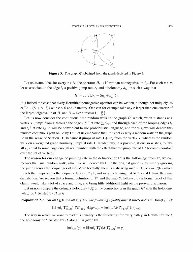
To explain this, let us consider a weighted graph with a well G. Let us associate to G a new graphG◦ = (V,E◦) which has the same vertices as G, and an extended set of edges
E◦ = E∪⋃x∈V
{lx , l−1x },
where the edge lx and its inverse have source and target x . We call these new edges looping edges.
COVARIANT SYMANZIK IDENTITIES 439
Figure 5. The graph G◦ obtained from the graph depicted in Figure 3.
Let us assume that for every x ∈ V, the operator Hx is Hermitian nonnegative on Fx . For each x ∈ V,let us associate to the edge lx a positive jump rate rx and a holonomy hlx , in such a way that
Hx = rx(2IdFx − (hlx + h−1lx)).
It is indeed the case that every Hermitian nonnegative operator can be written, although not uniquely, asr(2Id− (U +U−1)) with r > 0 and U unitary. One can for example take any r larger than one quarter ofthe largest eigenvalue of H, and U = exp i arccos
(1− H
2r
).
Let us now consider the continuous time random walk in the graph G◦ which, when it stands at avertex x , jumps from x through the edge e ∈ E at rate χe/λx , and through each of the looping edges lx
and l−1x at rate rx . It will be convenient to use probabilistic language, and for this, we will denote this
random continuous path on G◦ by 0◦. Let us emphasise that 0◦ is not exactly a random walk on the graphG◦ in the sense of Section 1E, because it jumps at rate 1+ 2rx from the vertex x , whereas the randomwalk on a weighted graph normally jumps at rate 1. Incidentally, it is possible, if one so wishes, to takeall rx equal to some large enough real number, with the effect that the jump rate of 0◦ becomes constantover the set of vertices.
The reason for our change of jumping rate in the definition of 0◦ is the following: from 0◦, we canrecover the usual random walk, which we will denote by 0, in the original graph G, by simply ignoringthe jumps across the loop-edges of G◦. More formally, there is a shearing map S : P(G◦)→ P(G) whichforgets the jumps across the looping edges of E◦ \E, and we are claiming that S(0◦) and 0 have the samedistribution. We reckon that a formal definition of 0◦ and the map S, followed by a formal proof of thisclaim, would take a lot of space and time, and bring little additional light on the present discussion.
Let us now compare the ordinary holonomy hol◦h of the connection h in the graph G◦ with the holonomyholh,H of h twisted by H in G.
Proposition 2.7. For all t ≥ 0 and all x, y ∈V, the following equality almost surely holds in Hom(Fx , Fy):
Ex [hol◦
h(0◦
|[0,t))|S(0◦
|[0,t))]1{0◦t =y} = holh,H (S(0◦|[0,t)))1{0◦t =y}.
The way in which we want to read this equality is the following: for every path γ in G with lifetime t ,the holonomy of h twisted by H along γ is given by
holh,H (γ )= E[hol◦h(0◦
t )|S(0◦
|[0,t))= γ ],

440 ADRIEN KASSEL AND THIERRY LÉVY
the average over a set of nonobserved paths in the larger graph G◦ of an ordinary unitary holonomy, andof which the observed path γ is an approximation.
Proof. Conditional on S(0◦|[0,t)) = ((x0, τ0), e1, . . . , (xn, τn)), the path 0◦
|[0,t) is equal to S(0◦|[0,t)) to
which have been grafted, at each of its stays at one of the vertices x1, . . . , xn , an independent Poissonianset of excursions through the loop-edges at this vertex.
For each k ∈ {0, . . . , n}, let Nk be an independent Poisson variable with parameter 2rxkτk and let βxk ,τk
be a random discrete loop of length Nk based at xk , which traverses Nk times one of the edges lx and l−1x
(and no other), independently with equal probability at each jump. Then
Ex [hol◦
h(X◦
|[0,t))|S(X◦
|[0,t))= ((x0, τ0), e1, . . . , (xn, τn))]
= E[hol◦h(βxn,τn )] ◦ hen ◦ E[hol◦h(βxn−1,τn−1)] ◦ · · · ◦ he1 ◦ E[hol◦h(βx0,τ0)].
On the other hand, for each k ∈ {0, . . . , n},
E[hol◦h(βxk ,τk )] = e−2rxk τk
∞∑n=0
(2rxkτk)n
n!12n
n∑m=0
(nm
)hm
lxkhn−m
l−1xk
= e−τkrxk (2IdFxk
−(hlxk+h−1
lxk))
= e−τk Hxk ,
and the expected result follows. �
2H. Occupation measures and local times. A particular case of interest of the twisted holonomy is thatwhere for every vertex x , the operator Hx is scalar. In this case, the twisted holonomy of a path can berelated to its occupation measure, or to its local time, which we now define.
Definition 2.8. Let γ = ((x0, τ0), e1, . . . , en, (xn, τn)) be a continuous path in the graph G. The occupationmeasure of γ is the measure ϑ(γ ) on V such that for every vertex x ,
ϑx(γ )=
n∑k=0
δx,xkτk .
The local time of γ is the density of its occupation measure with respect to the reference measure λ: forevery vertex x ,
`x(γ )=ϑx(γ )
λx=
1λx
n∑k=0
δx,xkτk .
From Section 6 on, we will consider Poissonian ensembles of paths. We will then use the followingextended definition of the occupation measures and local times: if P is a set of paths, we define, for everyvertex x ,
`x(P)=∑γ∈P
`x(γ ) and ϑx(P)=∑γ∈P
ϑx(γ ).
The following lemma is a straightforward consequence of the definition of the twisted holonomy. Inits statement, we use the same notation for a scalar operator and its unique eigenvalue.

COVARIANT SYMANZIK IDENTITIES 441
ex y
f(x) f(y)
he,x
he−1,y
df(e)
Fx Fe Fy
Figure 6. The computation of d f (e).
Lemma 2.9. Assume that for every vertex x , the operator Hx is scalar on Fx , that is, equal to Hx IdFx
for some Hx ∈ K. Let γ be a continuous path. Assume that τ(γ ) < +∞ or Hγ = 0. Then one has theequality
holh,H (γ )= e−∑
x∈V Hxϑx (γ )holh(γ ). (18)
This lemma shows how the twisted holonomy, which, in the classical language of the theory of Markovprocesses, could be called a multiplicative functional, extends the classical definition of exponentialfunctionals of local times.
2I. Differentials. Let us consider a graph G= (V,E), a vector bundle F over G and a connection h on F.
Definition 2.10. The differential is the linear operator
d :�0(F)→�1(F)⊂⊕e∈E
Fe
defined by setting, for every f ∈�0(F) and every e ∈ E,
(d f )(e)= he−1,e f (e)− he,e f (e).
The range of d is contained in �1(F); indeed, if the inverse of the edge e is defined, then replacing eby e−1 in this definition exchanges e and e, so that (d f )(e−1)=−(d f )(e) as expected. See Figure 6 foran illustration.
The definition of d depends on the connection h, but we prefer not to use the notation dh, which wefind too heavy.
Let us now assume that the graph G is a weighted graph with a well. Recall from (9) the notationPx,e = χe/λx .
Definition 2.11. The codifferential is the operator
d∗ :�1(F)→�0(F)

442 ADRIEN KASSEL AND THIERRY LÉVY
defined by setting, for all ω ∈�1(F) and all x ∈ U,
d∗ω(x)=∑
e∈E:e=x
Px,ehx,eω(e)=−∑
e∈E:e=x
Px,ehx,e−1ω(e). (19)
The following lemma justifies the notation that we used for the codifferential.
Lemma 2.12. The operators d and d∗ are adjoint of each other with respect to the Hermitian forms( · , · )�0 and ( · , · )�1 .
Let us emphasise that the proof of this lemma depends on the fact that the connection h consists ofunitary operators.
Proof. Let f ∈�0(U, F) and ω ∈�1(E, F). We have
( f, d∗ω)�0 =
∑x∈V
λx 〈 f (x), d∗ω(x)〉x
=12
∑x∈V
∑e∈E:e=x
χe〈 f (x), hx,eω(e)〉x −12
∑x∈V
∑e∈E:e=x
χe〈 f (x), hx,e−1ω(e)〉x
=12
∑e∈E
χe〈 f (e), h e,eω(e)〉e−12
∑e∈E
χe〈 f (e), he,e−1ω(e)〉e
=12
∑e∈E
χe〈he−1,e f (e), ω(e)〉e−12
∑e∈E
χe〈he,e f (e), ω(e)〉e
=12
∑e∈E
χe〈d f (e), ω(e)〉e = (d f, ω)�1 .
We used the unitarity of h between the third and the fourth line. �
2J. Laplacians. To the situation that we have been describing since the beginning of this paper, isassociated a Laplace operator, which is our main object of interest. A simple definition of this operator,acting on �0(F), would be the following:
1h = d∗ ◦ d ∈ End(�0(F)).
However, the Laplacian that we will use most of the time is the compression of this operator to thesubspace �0(V \W, F) of sections that vanish on the well (see Definition 2.2). In the following definition,we will use the notation πV\W, defined by (15), for the orthogonal projection of �0(F) onto �0(V \W, F).The adjoint π∗V\W of this projection is the inclusion of �0(V \W, F) into �0(F).
Definition 2.13. Let G be a weighted graph with a well. Let F be a vector bundle over G. Let h be aconnection on F. The h-Laplacian, or simply Laplacian, is defined on �0(V \W, F) as the linear mapping
1h = πV\W ◦ d∗ ◦ d ◦π∗V\W ∈ End(�0(V \W, F)).

COVARIANT SYMANZIK IDENTITIES 443
Consider f ∈�0(V \W, F) and choose x ∈ V \W. Thanks to (19), we have
(1h f )(x)=−∑
e∈E:e=x
Px,ehx,e−1(d f )(e)
=
∑e∈E:e=x
Px,e( f (x)− he−1 f (e))
= f (x)−∑
e∈E:e=x
Px,e1V\W(e)he−1 f (e). (20)
This last expression will be useful in the sequel.Using the Laplacian, we can define the Dirichlet energy functional on �0(V \W, F).
Definition 2.14. Let f be an element of �0(V \W, F). The Dirichlet energy of f is the real number
Eh( f )= ( f,1h f )�0 .
Remembering that an element of �0(V \W, F) is seen as a section of F over V vanishing over W, ashort computation yields
Eh( f )= 12
∑e∈E
χe‖ f (e)− he−1 f (e)‖2e, (21)
which makes it obvious that Eh( f ) is nonnegative.
Proposition 2.15. The operator 1h is Hermitian, nonnegative, and invertible on �0(V \W, F).
Proof. It follows from Lemma 2.12 that 1h = πV\W ◦ d∗ ◦ d ◦ πV\W is Hermitian and nonnegative on�0(V \W, F). There remains to prove that it is invertible.
Consider a section f such that 1h f = 0. Since f vanishes identically on the well, (21) and the factthat Eh( f )= 0 imply that f vanishes everywhere on V. �
In the special case of the trivial bundle KG over G endowed with the canonical connection (see the endof Section 2C), we will denote the Laplacian simply by 1.
2K. The smallest eigenvalue of the Laplacian. It follows from Proposition 2.15 that the lowest eigen-value of 1h is positive. In this section, we give a lower bound on this first eigenvalue. Let us define
σh =min Spec 1h = minf ∈�0(V\W,F)\{0}
( f,1h f )�0
( f, f )�0. (22)
On the trivial bundle K with the usual Laplacian 1, we denote this quantity by σ .
Proposition 2.16 (discrete Kato’s lemma). The following inequality holds:
σh ≥ σ > 0 .
Proof. The inequality σ > 0 is a special case of Proposition 2.15. Let us prove that σh ≥ σ . For this,consider a section f ∈�0(V \W, F). For all e ∈ E, we have
‖ f (e)− he−1 f (e)‖e ≥∣∣‖ f (e)‖e−‖he−1 f (e)‖e
∣∣= ∣∣‖ f (e)‖e−‖ f (e)‖e∣∣,
444 ADRIEN KASSEL AND THIERRY LÉVY
because he is unitary. Using (21), this implies the inequality
( f,1h f )�0 ≥ (‖ f ‖,1‖ f ‖) ,
where ‖ f ‖ is the function on V defined by ‖ f ‖(x) = ‖ f (x)‖x . Since ( f, f )�0 = (‖ f ‖, ‖ f ‖), theinequality σh ≥ σ follows. �
2L. Generalised Laplacians. We will consider linear operators on the space of sections of F that aresimilar to, but more general than the Laplacian 1h . In analogy with the case of a Hermitian vector bundleover a Riemannian manifold, for which there exists many second order differential operators with thesame symbol, which all deserve to be called Laplacians, and which differ by a term of order 0, we set thefollowing definition.
Recall from Definition 2.5 that we call potential a section of the vector bundle End(F) over V suchthat Hx is Hermitian (or, in the real case, symmetric) for each x ∈ V. There is a natural inclusion�0(End(F))⊂ End(�0(F)) thanks to which a potential can act on a section of F. Concretely, if H is apotential and f a section of F, then the section H f is simply defined by the fact that for all x ∈ V,
(H f )(x)= Hx( f (x)).
Definition 2.17. Let F be a Hermitian vector bundle over a graph with a well G, endowed with aconnection h. Let H be a potential on F. The generalised Laplacian on F associated to h and H, or(h, H)-Laplacian, is the following linear endomorphism of �0(V \W, F):
1h,H =1h + H.
Imitating Definition 2.14, we define the generalised Dirichlet energy of a section f as the number
Eh,H ( f )= ( f, (1h + H) f )�0 (23)
=12
∑e∈E
χe‖ f (e)− he−1 f (e)‖2e +∑x∈V
λx 〈 f (x), Hx f (x)〉x .
Recall from the previous section that we denote by σh the smallest eigenvalue of 1h , and that σh > 0. IfHx >−σh for every vertex x , then the operator 1h,H is invertible. This is in particular the case as soonas Hx ≥ 0 for every vertex x .
Let us conclude by describing the action of the gauge group on the operators that we just defined. Thegauge group acts naturally on �0(F): for all gauge transformations j and all sections f , the section j · fis defined by
( j · f )(x)= jx( f (x)).
This action extends to an action by conjugation on End(�0(F)): if B is an endomorphism of �0(F) andf is a section, then
( j · B)( f )= j · (B( j−1· f )).

COVARIANT SYMANZIK IDENTITIES 445
These actions allow us to express the way in which the Laplacians are acted on by the gauge group: withour current notation,
j ·1h,H =1 j ·h, j ·H . (24)
Since the gauge group acts on each fibre by unitary transformations, it follows that the Dirichlet energysatisfies
E j ·h, j ·H ( j · f )= Eh,H ( f ).
3. A covariant Feynman–Kac formula
3A. A Feynman–Kac formula. In this section, we will prove our first theorem, which is a version of theFeynman–Kac formula featuring holonomies, and which will be one of the most useful results for ourstudy. Recall the notion of twisted holonomy introduced in Definition 2.6.
Theorem 3.1 (Feynman–Kac formula). Let G be a weighted graph with a well. Let F be a vector bundleover G, endowed with a connection h and a potential H. Let X be the random walk on G defined inSection 1E.
Let f be an element of �0(V \W, F). For all x ∈ V \W and all t ≥ 0, the following equality holds:
(e−t1h,H f )(x)=∫P(G)
holh,H (γ−1|[0,t)) f (γt) dPx(γ ).
Note that since f vanishes identically on the well, the paths that reach the well before time t do notcontribute to the right-hand side.
Proof. We will use the fact that for any two endomorphisms A and B of a finite-dimensional vector spaceand all real t > 0,
et (A+B)=
∞∑k=0
∫0<t0<···<tk−1<t
et0 A Be(t1−t0)A · · · Be(t−tk−1)A dt0 · · · dtk−1,
a formula that can be checked by expanding the exponentials on the right-hand side in power series,computing the Eulerian integrals that appear, and observing that one recovers the left-hand side. In ourcontext, we use this formula in the following way: we first write e−t1h,H = e−t e−t H+t (Id−1h) and deducethat
e−t1h,H = e−t∞∑
k=0
∫0<t0<···<tk−1<t
e−t0 H (Id−1h)e−(t1−t0)H · · · (Id−1h)e−(t−tk−1)H dt0 · · · dtk−1.
Let f be a section of F and x a vertex of G. Using the expression (20) of 1h , we find
(e−t1h,H f )(x)= e−t∞∑
k=0
∑e1,...,ek∈E
Px,e1 Pe1,e2 · · · Pek−1,ek
k∏q=1
1V\W(eq)∫0<t0<···<tk−1<t
e−t0 Hx he−11
e−(t1−t0)He1 · · · he−1k
e−(t−tk−1)Hek f (ek) dt0 · · · dtk−1. (25)
446 ADRIEN KASSEL AND THIERRY LÉVY
On the other hand, according to (8) and (10),∫P(G)
holh,H (γ−1|[0,t)) f (γt) dPx(γ )
=
∑0≤k<n
p∈DPn(G)p=(x0,e1,...,en,xn)
Qx({p})∫
0<t0<···<tk−1<t<tk<···<tn−1
e−t0 Hx he−11
e−(t1−t0)Hx1
· · · he−1k
e−(t−tk−1)Hxk f (xk)e−tn−1 dt0 · · · dtn−1
= e−t∞∑
k=0
∑e1,...,ek∈E
Px,e1 Pe1,e2 · · · Pek−1,ek
k∏q=1
1V\W(eq)
( ∞∑l=0
∑e′1,...,e
′
l∈E
Pek ,e′1 Pe′1,e′
2· · · Pe′l−1,e
′
l1W(e′l)
l∏r=1
1V\W(e′r ))
∫0<t0<···<tk−1<t
e−t0 Hx he−11
e−(t1−t0)He1 · · · he−1k
e−(t−tk−1)Hek f (ek) dt0 · · · dtk−1.
The sum over l between the brackets is the total mass of the probability measure Qek , that is, 1, and werecover the right-hand side of (25). �
We will often use a slightly different, but equivalent, version of the Feynman–Kac formula. In order tostate it, let us introduce the following notation. The vector space of linear endomorphisms of �0(V\W, F)
is isomorphic to
End(�0(V \W, F))= End( ⊕
x∈V\W
Fx
)=
⊕x,y∈V\W
Hom(Fy, Fx).
This decomposition is nothing more than the block decomposition of the matrix representing an endo-morphism of �0(V \W, F), each block corresponding to one of the fibres of the bundle. For all linearoperator B ∈ End(�0(V \W, F)) and all x, y ∈ V, we will denote by Bx,y the linear map from Fy to Fx
which appears in the right-hand side of the decomposition above.Theorem 3.1 immediately implies the following.
Corollary 3.2. Under the assumptions of Theorem 3.1, and for all x, y ∈ V \W, the following equalityholds in Hom(Fy, Fx):
(e−t1h,H )x,y =
∫P(G)
holh,H (γ−1|[0,t))1{γt=y} dPx(γ ).
Provided we are careful enough about the source and target spaces of the linear operators that we arewriting, we can express the corollary in the following more compact form:
e−t1h,H =
⊕x∈V
(e−t1h,H )x,y =
∫P(G)
holh,H (γ−1|[0,t)) dPx(γ ).
COVARIANT SYMANZIK IDENTITIES 447
3B. The Green section. We devote this very short section to the definition of the analogue, in oursituation, of the Green function. For this, let us define the operator 3 on �0(F) such that for any section fand any vertex x ∈ V,
(3 f )(x)= λx f (x).
Recall from Section 2L that if Hx is a nonnegative Hermitian operator on Fx for every x ∈ V \W, thenthe operator 1h,H is invertible.
Definition 3.3. Let G be a weighted graph with a well. Let F be a fibre bundle over G. Let h be aconnection on F and H be a nonnegative potential on F. The Green section associated with h and H isthe operator
Gh,H = (3 ◦1h,H )−1∈ End(�0(V \W, F)).
According to (24), given a gauge transformation j of F, we have
j ·Gh,H = j ◦Gh,H ◦ j−1= G j ·h, j ·H . (26)
Let us make a brief comment about the distinction between sections and measures. The operator 3takes a section and multiplies it by a measure. The result of this operation is an object that can be pairedpointwise with a section, using the Hermitian scalar product of each fibre, thus producing a scalar functionthat can be integrated over the graph. It would thus be fair to say that 3 sends �0(F) into its dual space,and, since 1h,H is a genuine operator on �0(V \W, F), that Gh,H sends the dual of �0(V \W, F) into�0(V \W, F) itself. In a sense that we will not make very precise, the kernel of Gh,H is thus analogousto a function of two variables.
3C. Two elementary algebraic identities. The Feynman–Kac formula relates the semigroup of the gen-eralised Laplacian to the average of the twisted holonomy along the paths of the random walk in thegraph. In this paragraph, we will derive two consequences of this formula which will be the bases of ourproofs of the isomorphism theorems. The two formulas which we will now prove ultimately rely on thefollowing elementary lemma.
Lemma 3.4. Let A and B be two positive Hermitian matrices of the same size. Then∫∞
0e−t A dt = A−1 (27)
and ∫∞
0
e−t A− e−t B
tdt = log B− log A . (28)
Proof. It suffices to prove that for all positive real a,∫∞
0
e−ta− e−t
tdt =− log a .
Now, for all ε > 0,∫∞
εe−ta
t dt =∫∞
aεe−t
t dt and the integral that we want to compute is equal to∫ εaε
e−t
t dt =∫ ε
aε1t dt + O(ε), from which the result follows immediately. �

448 ADRIEN KASSEL AND THIERRY LÉVY
From the Feynman–Kac formula (Theorem 3.1), the definition of the measure ν (Definition 1.10),and (27), we deduce the following proposition.
Proposition 3.5. Assume that the potential H is nonnegative. For all x, y ∈ V \W the equality∫P(G)
holh,H (γ−1) dνx,y(γ )= (Gh,H )x,y (29)
holds in Hom(Fy, Fx). Moreover, we have the following equality in End(�0(V \W, F)):∫P(G)
holh,H (γ−1) dν(γ )=1−1
h,H . (30)
Similarly, from Theorem 3.1, Definition 1.11 and (28), we deduce the following.
Proposition 3.6. Let h, h′ be two connections on F and H, H ′ be two nonnegative potentials. We havethe following identity in End(�0(V \W, F)):∫
P(G)
(holh,H (γ−1)− holh′,H ′(γ
−1)) dµ(γ )= log1h′,H ′ − log1h,H . (31)
It turns out that (31) is difficult to use in its present form, and that it is often more convenient to usethe less detailed but still informative equation obtained from it by taking the trace of both sides. Here, bythe trace, we mean the usual trace in the space of endomorphisms of �0(V \W, F). Thus, if B is such anendomorphism, we call the trace of B the number
Tr(B)=∑
x∈V\W
TrFx (Bx,x).
Corollary 3.7. Let h be a connection and H a nonnegative potential. We have the identity∫L(G)
(Tr holh,H (γ−1)−Tr holh(γ−1)
)dµ (γ )= log
det1h
det1h,H. (32)
The reader may wonder why we wrote Proposition 3.6 as we did with a difference of holonomies,and what the integral of the twisted holonomy along a random path with respect to the measure µis. The answer is that this integral is ill defined, because of the presence of the infinite measure µwithin µ. However, it makes sense to compute this integral against µ−µ . The result is given by thenext proposition.
Proposition 3.8. Let h be a connection and H a nonnegative potential. In End(�0(V \W, F)), we havethe identity ∫
P(G)
holh,H (γ−1) d(µ−µ )(γ )=− log1h,H + log(Id+ H) . (33)
COVARIANT SYMANZIK IDENTITIES 449
Proof. Consider x and y in V. We have
l.h.s. of (33)=1λy
∫P(G)×(0,+∞)
hol(γ−1|[0,t))(1−1{γ|[0,t)=(x,t)}) dPx(γ )
dtt
=1λy
∫∞
0((e−t1h,H )x,y − δx,ye−t e−t Hx )
dtt
=1λy
(∫∞
0
e−t1h,H − e−t (Id+H)
tdt)
x,y.
Summing over y with respect to the reference measure λ and over x with respect to the counting measure,and using (28), we find the expected result. �
4. The Gaussian free vector field
In this section, we consider a weighted graph with a well G, over which we are given a vector bundle F
with a connection h and a potential H. In this setting, we will construct a Gaussian probability measureon �0(V \W, F).
From now on in this paper, we will always assume that potentials are nonnegative. In fact, whenever aconnection h is given, our results make sense and hold under the assumption that for all x ∈ V \W, onehas Hx >−σh , where σh is defined by (22).
4A. Probability measures on �0(V \ W,F). First, we will discuss Lebesgue measures on the space�0(V \W, F). Let us agree that the natural Lebesgue measure on a Euclidean or Hermitian space is thatwhich gives measure 1 to any real cube the edges of which have length 1. With this convention, there is anatural Lebesgue measure Leb�0 on �0(V \W, F) and, for each x ∈ V \W, a natural Lebesgue measureLebx on Fx . Considering the way in which the Euclidean or Hermitian structures on �0(V, F) on onehand and on the fibres of F on the other hand are related, through the measure λ (see Section 2B), we findthe equality
Leb�0 =
⊗x∈V\W
(λβ2 rx Lebx),
where, in order to treat the Euclidean and Hermitian cases simultaneously, we used the constant
β = dimR K, (34)
equal to 1 in the Euclidean case and to 2 in the Hermitian case.Let us denote by |V \W| the cardinality of V \W. We define the probability measure Ph,H on
�0(V \W, F) by setting
dPh,H ( f )=(
det1h,H
2πr |V\W|
) β2
e−12 ( f,1h,H f )
�0 dLeb�0( f ). (35)

450 ADRIEN KASSEL AND THIERRY LÉVY
We shall denote by 8 the canonical process (that is, the identity map) on �0(V \W, F), so that for allbounded measurable functions F :�0(V \W, F)→ R, we have
Eh,H[F(8)] =
∫�0(V,F)
F( f ) dPh,H ( f ).
The random section 8 is called the Gaussian free vector field, or simply Gaussian free field, on G
associated with h and H.We will often consider the Gaussian free vector field associated to a connection h and the zero potential.
In that case, we will use the notation Eh instead of Eh,0.
4B. Covariance. The measure Ph,H is Gaussian on�0(V\W, F) and we will now compute its covariancefunction. Let us introduce some notation which will be useful to express this covariance, and several ofthe results that we shall prove.
Consider a Euclidean or Hermitian vector space (V, ( · , · )). Recall that if V is Hermitian, we take theHermitian scalar product to be linear in the second variable. We define the conjugation map to be
V → V ∗, v 7→ v = (v, ·).
This map is an antilinear isomorphism between V and its dual V ∗, and it satisfies, for every scalar z andevery vector v, the relation zv = z v.
If V and W are Euclidean or Hermitian spaces, and if v and w are elements of V and W respectively,then w⊗ v is an element of W ⊗ V ∗ ' Hom(V,W ). More specifically, w⊗ v is the linear map of rank 1from V to W such that for all u ∈ V,
(w⊗ v)(u)= (v, u)w.
With this notation, a standard Gaussian computation yields the following identity.
Proposition 4.1. Let F be a vector bundle over G, endowed with a connection h and a potential H. Let 8be the associated Gaussian free vector field on G. Then
Eh,H[8⊗8] =1−1
h,H .
In other words, for all f, g ∈�0(V \W, F),
Eh,H[( f,8)�0(8, g)�0] = ( f,1−1
h,H g)�0 . (36)
Note that this formulation is true in the Euclidean case as well as in the Hermitian case.It is often useful to have an expression of the covariance of the values of the Gaussian free vector
field in two specific fibres of F. Passing from the space of sections to the individual fibres involves thereference measure λ, so that the inverse of the Laplacian will be replaced by the Green section.
Proposition 4.2. Let F be a vector bundle over G, endowed with a connection h and a potential H. Let 8be the Gaussian free vector field on G. Let Gh,H be the Green section of F. For all x, y ∈ V \W, we havethe following identity in Hom(Fy, Fx):
Eh,H[8x ⊗8y] = (Gh,H )x,y . (37)
COVARIANT SYMANZIK IDENTITIES 451
Proof. Let us choose two vertices x and y in V and two vectors ξ ∈Fx and η∈Fy . Applying Proposition 4.1to the sections f = ξ1{x} and g = η1{y}, which vanish respectively everywhere except at x and y, andsatisfy f (x)= ξ and g(y)= η, we find
λxλyEh,H[〈ξ,8x 〉x 〈8y, η〉y] = λx 〈ξ, (1
−1h,H )x,yη〉x .
This equality can be written
Eh,H[〈ξ,8x 〉x 〈8y, η〉y] = 〈ξ, (1
−1h,H3
−1)x,yη〉x ,
or even〈ξ, Eh,H
[8x ⊗8y]η〉x = 〈ξ, (Gh,H )x,yη〉x ,
which, because it is true for all ξ and η, implies the result. �
This proposition and (26) allow us to understand how the Gaussian free vector field transforms underthe action of a gauge transformation. Indeed, let us choose j ∈ Aut(F). For all vertices x, y and all ξ ∈ Fx
and η ∈ Fy , we have
Eh,H[〈ξ, jx(8x)〉x 〈 jy(8y), η〉y] = Eh,H
[〈 j−1x (ξ),8x 〉x 〈8y, j−1
y (η)〉y]
= 〈ξ, ( jx ◦ (Gh,H )x,y ◦ j−1y )(η)〉x
= 〈ξ, (G j ·h, j ·H )x,y(η)〉x
Thus, if 8 is the Gaussian free vector field associated to the pair (h, H) and if j is a gauge transformation,then the Gaussian free vector field associated to the pair ( j · h, j · H) has the same distribution as j (8).
4C. Laplace transform. For future reference, let us record the Laplace transform and a formula for thehigher moments of the Gaussian free vector field. We keep the notation of the previous section.
The next proposition follows from (36) and the standard computation of a Gaussian integral. Note thatit is written in such a way as to be true in the real case as well as in the complex case.
Proposition 4.3. For all f ∈�0(V \W, F), we have
Eh,H[|e
12 ( f,8)
�0 |2] = e
12 ( f,1−1
h,H f )�0 .
The following formula, which is a reformulation of Wick’s theorem (see [Janson 1997]) in our context,combined with (30), will be useful in the proof of the covariant Symanzik identity (Theorem 7.3). It isone of the results where the real and complex case are quite different.
Proposition 4.4. Assume K = R. Then, for any integer k ≥ 0 and all sections f1, . . . , fk ∈�0(V \W, F),
we have
Eh,H[ k∏
i=1
( fi ,8)�0
]=
∑π
∏{i, j}∈π
∫P(G)
λγ 〈 fi (γ ), holh,H (γ−1) f j (γ )〉γ dν(γ ), (38)
where the sum is over all partitions of the set {1, . . . , k} by pairs. In particular, this expectation is zeroif k is odd.
452 ADRIEN KASSEL AND THIERRY LÉVY
Assume that K = C. Then, for all integers k, l ≥ 0, all f1, . . . , fk and f ′1, . . . , f ′l in �0(V \W, F), wehave
Eh,H[ k∏
i=1
( fi ,8)�0
l∏j=1
(8, f ′j )�0
]=
∑σ
k∏i=1
∫P(G)
λγ 〈 fi (γ ), holh,H (γ−1) f ′σ(i)(γ )〉γ dν(γ ), (39)
where the sum is over all bijections from {1, . . . , k} to {1, . . . , l}. In particular, this expectation is zero ifk 6= l.
4D. Square of the shifted Gaussian free vector field. In this section, and in preparation for the proofof Theorem 6.6, we record a useful lemma which expresses the Laplace transform of the square of theshifted Gaussian free vector field. This is a generalisation of [Sznitman 2012b, Proposition 2.14] to thepresent covariant setting.
Proposition 4.5. Let h be a connection and H a potential on F. For all f ∈�0(V \W, F), we have
Eh[e−
12 (8+ f,H(8+ f ))
�0 ] = Eh[e−
12 (8,H8)�0 ]e
12 (1h f,(1−1
h,H−1−1h )1h f )
�0 . (40)
Proof. Let us compute the left-hand side of the equality to prove. We will successively apply thedefinition (35) of the measure Ph, writing dϕ instead of dLeb�0(ϕ), then perform the usual completion ofthe square, then use the invariance by translation of the Lebesgue measure. We find(πr |V|
det1h
)β2
Eh[e−
12 (8+ f,H(8+ f ))
�0 ] =
∫�0(V\W,F)
e−12 (ϕ+ f,H(ϕ+ f ))
�0 e−12 (ϕ,1hϕ)�0 dϕ
=
∫�0(V\W,F)
e−12 (ϕ+1
−1h,H H f,1h,H (ϕ+1
−1h,H H f ))
�0 dϕ e12 ( f,(H1−1
h,H H−H) f )�0
=
∫�0(V\W,F)
e−12 (ϕ,1h,Hϕ)�0 dϕ e
12 (1h f,(1−1
h,H−1−1h )1h f )
�0 .
In the second exponential of the last line, we used the equality
a(a+ b)−1a− a = (a+ b− b)(a+ b)−1(a+ b− b)− a = b(a+ b)−1b− b
which is true in any associative algebra and that we applied in this instance to a = H and b =1h in thealgebra End(�0(V \W, F)).
Now, in the integral on the right-hand side we recognise, up to the normalisation factor by which wemultiplied both sides, the expectation on the right-hand side of (40). �
5. Isomorphism theorems of Dynkin and Eisenbaum
In this section, we explain how the two classical isomorphism theorems of Dynkin [1984a] and Eisenbaum[1995] extend to the present setting, in a way which incorporates the geometry of the vector bundle overthe graph. Our main tool will be the following combination of (29) and (37), which reads, for any two

COVARIANT SYMANZIK IDENTITIES 453
vertices x and y of a weighted graph with a well,
Eh,H[8x ⊗8y] = (Gh,H )x,y =
∫P(G)
holh,H (γ−1) dνx,y(γ ). (41)
5A. Dynkin’s isomorphism. Our generalisation of Dynkin’s isomorphism is the following. We use thenotation
∫νx,y
to denote the integral with respect to the finite measure νx,y . Recall from (34) the definitionof the constant β.
Theorem 5.1. Let G be a weighted graph with a well. Let F be a Hermitian or Euclidean vector bundleover G. Let h be a connection on F and H a potential on F. For all vertices x, y of V \W, the followingidentity holds in Hom(Fy, Fx):
Eh⊗∫νx,y[e−
12 (8,H8)�0 holh,H (γ
−1)] = Eh[e−
12 (8,H8)�0 8x ⊗8y] . (42)
In particular, if ξ ∈ Fx and η ∈ Fy ,
Eh⊗∫νx,y[e−
12 (8,H8)�0 〈ξ, holh,H (γ
−1)(η)〉x ] = Eh,H[〈ξ,8x 〉x 〈8y, η〉y] (43)
Proof. By definition of the measure Ph,H, we have
Eh[e−
12 (8,H8)�08x ⊗8y]
Eh[e−12 (8,H8)�0 ]
= Eh,H[8x ⊗8y] ,
which equals∫νx,y[holh,H (γ
−1)] by (41). The result follows immediately. �
Let us explain how successive specialisations of this theorem will allow us to recover Dynkin’sisomorphism in its classical version. Let us consider first the case where H is a scalar potential, that is, thecase where for each vertex x ∈ V, the operator Hx has a unique eigenvalue, which we also denote by Hx .In that case, according to Lemma 2.9, the twisted holonomy along a continuous path can be expressed interms of its classical holonomy and an exponential functional of its local time, and (42) becomes
Eh⊗∫νx,y
[e−
12∑
x∈V λx Hx (‖8x‖2+`x (γ ))holh(γ
−1)]= Eh[e− 1
2∑
x∈V λx Hx‖8x‖28x ⊗8y
].
Going one step further in the specialisation, let us apply this formula to the case of the trivial real bundleof rank 1 endowed with the trivial connection. In that case, 8 is a random real valued function on V \W
and we find one of the classical formulations of Dynkin’s isomorphism, namely
E⊗∫νx,y[e−
12∑
x∈V λx Hx (|8x |2+`x (γ ))] = E[e−
12∑
x∈V λx Hx |8x |28x8y].
It appears that Dynkin’s theorem is one of these deep results that, with the benefit of a few decades ofhindsight and the appropriate set of preliminary definitions, become almost tautological. Nevertheless,from our point of view, it remains definitely not trivial in that it expresses the covariance of the Gaussianfree vector field as a weighted sum of holonomies along paths in our graph. For example, if we pick avertex x , then the covariance matrix of the random vector 8x in the vector space Fx is given by
Eh,H[8x ⊗8x ] =
∫L(G)
holh,H (γ−1) dνx,x(γ ) ∈ End(Fx).
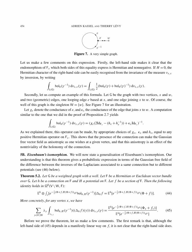
454 ADRIEN KASSEL AND THIERRY LÉVY
x w
e
e−1
Figure 7. A very simple graph.
Let us make a few comments on this expression. Firstly, the left-hand side makes it clear that theendomorphism of Fx which both sides of this equality express is Hermitian and nonnegative. If H = 0, theHermitian character of the right-hand side can be easily recognised from the invariance of the measure νx,x
by inversion, by writing∫L(G)
holh(γ−1) dνx,x(γ )=
∫L(G)
12(holh(γ )+ holh(γ )
−1) dνx,x(γ ).
Secondly, let us compute an example of this formula. Let G be the graph with two vertices, x and w,and two (geometric) edges, one looping edge e based at x , and one edge joining x to w. Of course, thewell of this graph is the singleton W = {w}. See Figure 7 for an illustration.
Let χe denote the conductance of e, and κx the conductance of the edge that joins x tow. A computationsimilar to the one that we did in the proof of Proposition 2.7 yields∫
L(G)
holh(γ−1) dνx,x(γ )= (χe(2IdFx − (he+ h−1
e ))+ κx IdFx )−1.
As we explained there, this operator can be made, by appropriate choices of χe, κx and he, equal to anypositive Hermitian operator on Fx . This shows that the presence of the connection can make the Gaussianfree vector field as anisotropic as one wishes at a given vertex, and that this anisotropy is an effect of thenontriviality of the holonomy of the connection.
5B. Eisenbaum’s isomorphism. We will now state a generalisation of Eisenbaum’s isomorphism. Ourunderstanding is that this theorem gives a probabilistic expression in terms of the Gaussian free field ofthe difference between the inverses of the Laplacians associated to a same connection but to differentpotentials (see (46) below).
Theorem 5.2. Let G be a weighted graph with a well. Let F be a Hermitian or Euclidean vector bundleover G. Let h be a connection on F and H a potential on F. Let f be a section of F. Then the followingidentity holds in �0(V \W, F):
Eh⊗∫ν[e−
12 (8+ f,H(8+ f ))
�0holh,H (γ−1)]1h f = Eh
[e−12 (8+ f,H(8+ f ))
�0 (8+ f )]. (44)
More concretely, for any vertex x , we have∑y∈V\W
λy
∫νx,y
holh,H (γ−1)((1h f )(y)) dνx,y(γ )=
Eh[e−
12 (8+ f,H(8+ f ))
�0 (8x + fx)]
Eh[e−12 (8+ f,H(8+ f ))
�0 ]
. (45)
Before we prove the theorem, let us make a few comments. The first remark is that, although theleft-hand side of (45) depends in a manifestly linear way on f , it is not clear that the right-hand side does.

COVARIANT SYMANZIK IDENTITIES 455
This is however the case, as will be clear from the proof. This feature is shared by Eisenbaum’s originalstatement, which we shall deduce from our theorem later.
A second remark is that one of the prominent features of Eisenbaum’s theorem, namely the use ofunconditioned measures on the trajectories of the Markov process, seems to have disappeared in ourstatement. We shall explain below how to fill this apparent gap between our formulation and Eisenbaum’soriginal statement.
A third remark is that, in the right-hand side of (45), f can be taken out of the expectation, thusproducing, thanks to (30), a statement of the form
1−1h,H1h f = f + · · ·
where the dots hide a nonobviously linear functional of f . Applying this formula not to f but to 1−1h f ,
we find
1−1h,H f =1−1
h f +Eh[e−
12 (8+1
−1h f,H(8+1−1
h f ))�08]
Eh[e−12 (8+1
−1h f,H(8+1−1
h f ))�0 ]
, (46)
the announced probabilistic expression of the difference between the inverses of two Laplacians.Let us now turn to the proof of the theorem.
Proof. Using successively (30) and Proposition 4.1, we find(∫P(G)
holh,H (γ−1) dν(γ )1h f
)(x)=1−1
h,H (1h f )(x)= Eh,H[(8,1h f )�08x ].
We now use the following Gaussian lemma. Let (X, Y ) be an (r+1)-dimensional Gaussian vector suchthat X is r-dimensional and Y is 1-dimensional. Assume that the vector (X, Y ) is symmetric, that is,centred in the real case, and, in the complex case, such that (eiθ X, eiθY ) has the same distribution as(X, Y ) for every real θ . Then, denoting by <Y the real part of Y,
E[Y X ] =E[e<Y X ]E[e<Y ]
.
We apply this lemma X =8x and Y = (1h f,8)�0 . The Gaussian vector (X, Y ) is symmetric because 8and −8 have the same distribution and, in the complex case, the same distribution as eiθ8 for all real θ .We find (∫
P(G)
holh,H (γ−1) dν(γ )1h f
)(x)=
Eh,H[e<(8,1h f )
�08x ]
Eh,H [e<(8,1h f )�0 ]
.
Replacing, by an affine change of variables, 8 by 8+ f in the numerator and the denominator, we findthat this quotient is equal to
Eh,H[e−<(8,H f )
�0 (8x + fx)]
Eh,H [e−<(8,H f )�0 ]
=Eh[e−
12 (8+ f,H(8+ f ))
�0 (8x + fx)]
Eh[e−12 (8+ f,H(8+ f ))
�0 ]
,
as expected. �

456 ADRIEN KASSEL AND THIERRY LÉVY
The next lemma will help us to bridge the gap between Theorem 5.2 and Eisenbaum’s originalisomorphism. In order to state it, recall from (6) the following notation: for every continuous path γ ,
τ(γ )= inf{t ≥ 0 : γt ∈W}
is the hitting time of the well by γ .
Lemma 5.3. Let x be a proper vertex of G. Let F be a nonnegative measurable function on P(G). Then∑y∈V\W
κy
∫P(G)
F(γ ) dνx,y(γ )=
∫P(G)
F(γ|[0,τ (γ ))) dPx(γ ).
Proof. Let us compute the left-hand side. It is equal to
∑y∈V\W
κy
λy
∫∞
0e−t
∞∑n=0
∑(x,e1,x1,...,xn−1,en,y)∈DPn(G)
Px,e1 Px1,e2 · · · Pxn−1,en∫0<t1<···<tn<t
F((x, t1), e1, (x1, t2− t1), . . . , (y, t − tn)) dt1 · · · dtn,
that is, to∑(x,e1,...,y)∈DPn(G)
e∈E:e=y,e∈W
Qx((x, e1, . . . , y, e, e))∫(0,+∞)n+1
F((x, τ0), e1, . . . , (y, τn))e−τ0−···−τn dτ0 · · · dτn,
in which we recognise the right-hand side. �
Using this lemma, we will now state a corollary of Theorem 5.2 from which it will be easy to deducethe classical statement.
Let us introduce the operator K on �0(V \W, F) defined by
(K f )(x)= κx f (x).
Corollary 5.4. Let F be a Hermitian vector bundle over a weighted graph with a well G. Let h be aconnection on F and H a potential on F. Let x be a vertex of G. Let b be a section of F over ∂(V \W).Define a global section f of F over V by setting
f = Gh K b.
Then the following identity holds in Fx :
Eh⊗ Ex
[e−
12 (8+ f,H(8+ f ))
�0holh,H (γ−1|[0,τ (γ )))(b)
]= Eh[e− 1
2 (8+ f,H(8+ f ))�0 (8x + fx)
]. (47)
Note that the path γ−1[0,τ (γ )) does not start from a vertex of the well, but instead from the last proper
vertex visited by γ before hitting the well. This last visited proper vertex belongs to the set ∂(V \W),which is precisely the set where b is defined.

COVARIANT SYMANZIK IDENTITIES 457
Proof. According to Lemma 5.3 and (41),
Ex [holh,H (γ|[0,τ (γ )))−1)(b)] = (Gh,H K b)(x)=1−1
h,H1h f,
which, given (30), is computed by Theorem 5.2. �
Just as in the case of Dynkin’s isomorphism, this result can be specialised to the original versionof Eisenbaum’s isomorphism. Assume that H is scalar in each fibre Fx , equal to Hx IdFx . In that case,observing that the full trajectory of the random walk and the trajectory stopped at the hitting time of thewell have the same local time at every vertex of V, (47) becomes
Eh⊗ Ex
[e−
12∑
x∈V\W λx Hx (‖8x+ fx‖2+`x (γ ))holh(γ
−1|[0,τ (γ )))(b)
]= Eh[e− 1
2∑
x∈V\W λx Hx‖8x+ fx‖2(8x + fx)
].
Assume now that the fibre bundle is the trivial real bundle of rank 1 and the connection is the trivialconnection. Let b be the section, that is, the function, which is identically equal to a real number s on∂(V \W). In that case, f = G K b = sGκ = s1V, the function identically equal to s on V \W. Then theformula above becomes
E⊗ Ex [e−12∑
x∈V\W λx Hx ((8x+s)2+`x (X))]s = E[e−12∑
x∈V\W λx Hx (8x+s)2(8x + s)].
Provided s is not zero, dividing by s yields one of the classical formulations of Eisenbaum’s isomorphism.Let us finally explain how the results of this section can be understood in terms of the resolution of a
Dirichlet problem in G.Recall from the beginning of Section 2J that there exists an uncompressed Laplacian 1h = d∗ ◦ d
acting on the space �0(V, F) of all sections of F, even those that do not vanish on the well. Adding apotential H to this Laplacian, we obtain the operator 1h,H =1h + H.
Suppose that we are given a section w ∈�0(W, F) of F over the well and we want to solve the Dirichletproblem with this boundary condition, that is, to find a section f ∈�0(V, F) of F such that{
1h,H f = 0 on V \W,
f = w on W.(48)
Assuming that H vanishes on the well as usual, the Laplacians 1h,H and 1h,H agree everywhere but onthe rim and for every x ∈ ∂(V \W), we have
1h,H f (x)=1h,H f (x)−∑
e=x,e∈W
h−1e f (e).
Thus, f solves the Dirichlet problem (48) if and only if it is satisfies
1h,H f (x)=
{0 if x ∈ (V \W) \ ∂(V \W),
b if x ∈ ∂(V \W),(49)
where b is the section of F over ∂V defined by
b(x)=∑
e=x,e∈W
h−1e w(e).

458 ADRIEN KASSEL AND THIERRY LÉVY
It appears that solving the Dirichlet problem for the uncompressed Laplacian in the graph with a boundarycondition on the well amounts to applying the inverse of the compressed Laplacian to a certain sectionof F over the rim.
It is a classical fact that the solution of the Dirichlet problem in a domain with a certain boundarycondition is the average of the Gaussian free field on this domain conditioned to satisfy this boundarycondition. The relation (46) extends this result in the following sense: provided one knows how to solvethe Dirichlet problem associated with the Laplacian 1h for a certain boundary condition, this corollarygives an expression in terms of the Gaussian free field of the solution of the Dirichlet problem with thesame boundary condition but for any of the generalised Laplacians 1h,H .
6. Isomorphism theorems of Le Jan and Sznitman
In this section, we continue our investigation of the way in which classical isomorphism theorems can beextended to the covariant setting and we turn to Le Jan’s and Sznitman’s isomorphism theorems, whichrelate the magnitude of the Gaussian free vector field to local times of Poissonian ensembles of loops andpaths.
Just as our approach to the generalisation of the isomorphism theorems of Dynkin and Eisenbaum wasbased on one main equality, namely (30), the results of this section will ultimately be based on (31). Inparticular, the measure µ in its various forms (see Definition 1.11) will play a prominent role in this study.
However, (31) turns out to be more difficult to use than (30) and we use instead the traced versionof (31), namely (32), which we recall here for the convenience of the reader:∫
L(G)
(Tr holh,H (γ−1)−Tr holh(γ−1))dµ (γ )= logdet1h
det1h,H. (50)
Using the definition of the measure µ , this equality can be written∑x∈V
∫∞
0
∫L(G)
(TrFx (holh,H (γ
−1|[0,t)))−TrFx (holh(γ
−1|[0,t)))
)1{γt=x} dPx(γ )
dtt= log
det1h
det1h,H. (51)
6A. Overview of the approach. Let us explain, in the Euclidean case, and with Le Jan’s theorem in mind,how we are going to use (50). Firstly, we are going to exponentiate it and recognise, in the right-handside, the expectation Eh
[e−12 (8,H8)�0 ]. The problem is to interpret the left-hand side
exp∫L(G)
(Tr holh,H (γ−1)−Tr holh(γ−1))dµ (γ ). (52)
A probabilistic interpretation of this quantity relies on Campbell’s formula for Poisson point processes,which goes as follows. Given a nonatomic σ -finite Borel measure m on a Polish space X , let us denoteby X the Poisson point process on X with intensity m. Then the Campbell formula (see for instance[Kingman 1993]) asserts that for every Borel function f on X such that f ≥ 1,
E
[∏x∈X
f (x)]= exp
∫X( f − 1) dm.

COVARIANT SYMANZIK IDENTITIES 459
In order to put (50) in the form of Cambpell’s formula, we will proceed as follows. Firstly, we will usethe fact that the measure µ is invariant under the path reversal map γ 7→ γ−1 (see Lemma 1.13) and thefact that the twisted holonomy is turned into its adjoint by composition by the same map (see (17)), to saythat the imaginary part of the integral in (50) vanishes and that we can replace traces by their real parts.
The second step one would like to take is a simple algebraic manipulation leading to the form
exp∫L(G)
(<Tr holh,H (γ−1)
<Tr holh(γ−1)− 1
)d(<Tr holh(γ−1)µ ). (53)
This form has two drawbacks. The first is that the quotient of real part of traces is difficult to interpret.With [Le Jan 2011] in mind, we would like to understand it as the exponential of some linear functionalof H and the local time of γ . However, the noncommutativity of the present setting makes it difficultto extract from this quotient the contribution of H. The second drawback is the fact that we are nowintegrating with respect to a signed measure. In certain specific situations, it so happens that the trace ofthe holonomy along any loop is nonnegative; we will give an example of such a situation in Section 6H.But in general, we will simply write the signed measure as the difference of two positive measures, anduse Campbell’s formula for each of them. We will thus obtain a quotient of two instances of Campbell’sformula.
On the other hand, we offer a solution to the problem of the interpretation of the quotient of real partsof traces of holonomies. It consists in lifting the integral from the space of loops to a larger space, onwhich holonomies, or rather quotients of holonomies, become scalar quantities. This requires a detailedexplanation, which will occupy us for the next few sections.
6B. Splitting of vector bundles. The main new piece of structure that we need in our study of Le Jan’sand Sznitman’s isomorphisms is a decomposition of each fibre of the vector bundle F as an orthogonaldirect sum of linear subspaces.
Definition 6.1. Let G be a graph. Let F be a vector bundle over G. A splitting of F, or colouring of F, isa collection I= {(Ix , (F
ix)i∈Ix ) : x ∈ V} in which, for each x ∈ V, Ix is a set and {Fi
x : i ∈ Ix} is a familyof pairwise orthogonal linear subspaces of Fx such that
Fx =
⊥⊕i∈Ix
Fix . (54)
For each x ∈ V and i ∈ Ix , we denote by π ix : Fx → Fi
x the orthogonal projection.
A special case of splitting is the trivial splitting, in which each fibre of F is simply written as being equalto itself. As trivial as it is, this splitting will be useful for us, and we will denote it by T={({x}, Fx) : x ∈V}.
Another special case is the case of complete splittings, in which each fibre is written as an orthogonaldirect sum of lines.
There is a natural partial ordering of the set of all splittings of a fibre bundle: we say that the splitting I
is finer than the splitting I′ if for each vertex x and each i ∈ Ix , there exists i ′ ∈ I ′x such that Fix ⊂ Fi ′
x . Thetrivial splitting is the maximum of this order, and the complete splittings are its minimal elements.

460 ADRIEN KASSEL AND THIERRY LÉVY
We say that a splitting I and a potential H on F are adapted to each other if for all x ∈ V and all i ∈ Ix ,the space Fi
x is an eigenspace of Hx . In this case, we will denote by H ix the unique eigenvalue of the
restriction of Hx to Fix , so that for all x ∈ V, we have
Hx =∑i∈Ix
H ixπ
ix .
For example, to say that a potential is adapted to the trivial splitting means that it is scalar on eachfibre. This is a kind of potential that we already considered twice, in order to specialise Theorems 5.1and 5.2 respectively to the classical Dynkin and Eisenbaum isomorphisms.
To every potential H we can associate its eigensplitting, the splitting of F obtained by writing eachfibre Fx as the direct sum of the eigenspaces of Hx . This splitting is of course adapted to H and it is,among all splittings adapted to H, the one that is maximal for the partial order that we just described.
6C. Splitting of the Gaussian free vector field. A splitting of F allows us, among other things, to splitthe Gaussian free vector field on G.
Let h be a connection and H be a potential on our vector bundle F over G. Let 8 be the Gaussian freevector field on F associated to h and H. Let I be a splitting of F. For each vertex x and each i ∈ Ix , wedefine
8ix = π
ix(8x). (55)
We meet here for the first time a new kind of field, namely (8ix)x∈V\W,i∈Ix , indexed not only by the
vertices of G, but also, at each vertex x , by elements of Ix , which we will call colours. Without givingtoo precise a meaning to this term, we will speak of a coloured field.
This coloured field (8ix)x∈V\W,i∈Ix is a Gaussian random element of
⊕x∈V\W,i∈Ix
Fix . It is centred,
and an application of (37) allows us to compute its covariance: for all x, y ∈ V\W and all i ∈ Ix , j ∈ Iy ,
Eh,H[8i
x ⊗8jy] = π
ix ◦ (Gh,H )x,y ◦π
jy , (56)
an equality to be read in Hom(F jy, F
ix).
The case where I is a complete splitting is of particular interest. Let us consider this case, and let usalso assume that the set of colours Ix is the same for each vertex x ∈ V, namely Ix = {1, . . . , r}. Letus finally choose a unit vector ui
x in each line Fix . Then, for each i ∈ {1, . . . , r}, we can define a scalar
random field 8i on V by setting, for all x ∈ V, and with a conflict of notation that we do not deem tooserious,
8ix = 〈u
ix ,8x 〉x .
Each of the r scalar fields 8i , i ∈ {1, . . . , r} is a centred Gaussian field and for all i ∈ {1, . . . , r}, thecovariance of the scalar field 8i is given, for all x, y ∈ V, by
Eh,H[8i
x8iy] = 〈u
ix , (Gh,H )x,yui
y〉x .
Although this is clear from (56), we would like to stress that the fields 81, . . . , 8r are genericallycorrelated, due to the presence of the connection h and the potential H (see Figure 8).
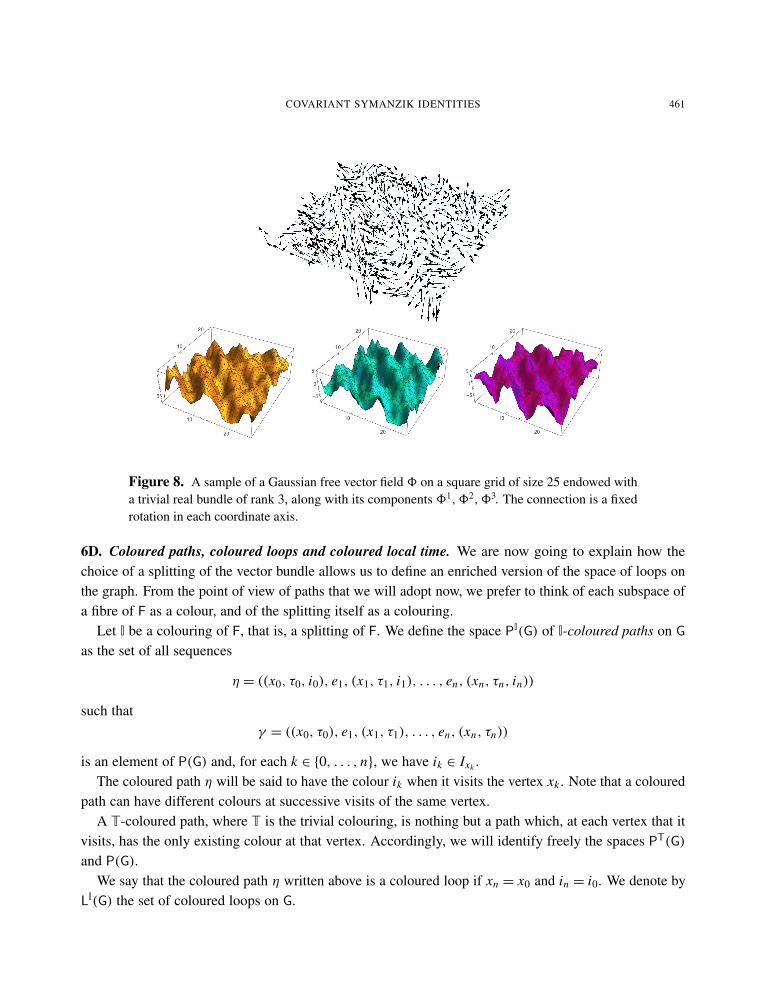
COVARIANT SYMANZIK IDENTITIES 461
Figure 8. A sample of a Gaussian free vector field 8 on a square grid of size 25 endowed witha trivial real bundle of rank 3, along with its components 81,82,83. The connection is a fixedrotation in each coordinate axis.
6D. Coloured paths, coloured loops and coloured local time. We are now going to explain how thechoice of a splitting of the vector bundle allows us to define an enriched version of the space of loops onthe graph. From the point of view of paths that we will adopt now, we prefer to think of each subspace ofa fibre of F as a colour, and of the splitting itself as a colouring.
Let I be a colouring of F, that is, a splitting of F. We define the space PI(G) of I-coloured paths on G
as the set of all sequences
η = ((x0, τ0, i0), e1, (x1, τ1, i1), . . . , en, (xn, τn, in))
such thatγ = ((x0, τ0), e1, (x1, τ1), . . . , en, (xn, τn))
is an element of P(G) and, for each k ∈ {0, . . . , n}, we have ik ∈ Ixk .The coloured path η will be said to have the colour ik when it visits the vertex xk . Note that a coloured
path can have different colours at successive visits of the same vertex.A T-coloured path, where T is the trivial colouring, is nothing but a path which, at each vertex that it
visits, has the only existing colour at that vertex. Accordingly, we will identify freely the spaces PT(G)
and P(G).We say that the coloured path η written above is a coloured loop if xn = x0 and in = i0. We denote by
LI(G) the set of coloured loops on G.

462 ADRIEN KASSEL AND THIERRY LÉVY
By analogy with Definition 2.8, we define, for all x ∈ V and all i ∈ Ix , the occupation measure and thelocal time of η with colour i at the vertex x ∈ V by
ϑ ix(η)=
n∑k=0
δx,xkδi,ikτk and `ix(η)=
1λxϑ i
x(γ ).
In our naive quantum mechanical picture of paths on the graph, a coloured path describes not onlythe motion of a particle, but the successive states in which this particle can be found at the successivevertices that it visits. If the splitting that we are considering is the eigensplitting of a potential H, thenthese states can be measured at each vertex x by the observable Hx .
Let us conclude this section by saying something about the way in which the set of I-coloured pathsdepends on the colouring I. Let us consider two colourings I and I′ of F such that I is finer than I′.Extending the metaphor of colours, there is a bleaching map bI′,I : P
I(G)→ PI′(G) which, at each vertex xvisited by a path, changes the colour i ∈ Ix into the unique colour i ′ ∈ I ′x such that Fi
x ⊂ Fi ′x . If I′′ is a
third colouring such that I′ is finer than I′′, then the relation bI′′,I′ ◦ bI′,I = bI′′,I holds.The special case where I′ is the trivial colouring will be of particular interest, and we will use the
simpler notation [η] = bT,I(η) for the element of P(G) obtained by forgetting altogether the colours of anI-coloured path η.
6E. Amplitudes. We will now use the colourings of a path to decompose the trace of the holonomyalong that path, and ultimately to simplify the expression (53).
Let I be an arbitrary colouring and let η = ((x0, τ0, i0), e1, (x1, τ1, i1), . . . , en, (xn, τn, in)) be an I-coloured path. Recall that we chose a connection h and a potential H on the vector bundle F. We definethe amplitude of h along the I-coloured path η twisted by H as the operator
ampIh,H (η)= π
inxn◦ e−τn Hxn ◦ hen ◦ · · · ◦π
i1x1◦ e−τ1 Hx1 ◦ he1 ◦π
i0x0◦ e−τ0 Hx0 : Fi0
x0→ Fin
xn.
This definition is designed for the following equality to hold: for every (noncoloured) path γ ,∑η∈PI(G):[η]=γ
ampIh,H (η)= holh,H (γ ) , (57)
where holh,H was defined in Definition 2.6. More generally, if I is finer than I′, then for all η′ ∈ PI′(G),∑η∈PI(G):bI′,I(η)=η
′
ampIh,H (η)= ampI′
h,H (η′) . (58)
Note that for every I-coloured path η, we have
ampIh,H (η
−1)= ampIh,H (η)
∗, (59)
the adjoint of ampIh,H (η). In particular, if η is a coloured loop, then the traces Tr ampI
h,H (η) andTr ampI
h,H (η−1) are conjugate complex numbers.
One of the reasons to introduce amplitudes is the following: if H and I are adapted, then
ampIh,H (η)= e−
∑x∈V\W,i∈Ix H i
xϑix (η)ampI
h(η), (60)

COVARIANT SYMANZIK IDENTITIES 463
a formula analogous to (18), but which holds without the assumption that H be scalar in each fibre. Thisindicates that, after lifting (53) from L(G) to LI(G), it will be much easier to deal with the quotient ofholonomies, which will become a quotient of amplitudes. Before we implement this lifting procedure, wemust say a word about the measures, indeed the signed measures that we will use on LI(G) and PI(G).
6F. Signed measures on the sets of coloured loops and paths. In this section, we will define two familiesof measures on sets of coloured paths. Firstly, we will define a signed measure µ ,I
h on the set of I-colouredloops, which in a sense lifts a measure on the set of loops absolutely continuous with respect µ (seeDefinition 1.11), with a density depending on the connection h. Then, for every section f of F, we willdefine a signed measure νI
h, f on the set of I-coloured paths, which in a similar sense lifts and generalisesthe measures νx,y (see Definition 1.10).
Definition 6.2. Let h be a connection on F. Let I be a colouring of F. The measure µ ,Ih is defined on
LI(G) by the fact that for all bounded nonnegative measurable functions F on LI(G),∫LI(G)
F(η) dµ ,Ih (η)=
∫L(G)
∑η∈LI(G):[η]=γ
F(η)<Tr(ampIh(η−1)) dµ (γ ).
To make it clear that the integral above exists, we can rewrite it as∫L(G)
∑η∈LI(G):[η]=γ
F(η)<Tr(ampIh(η−1)) dµ (γ )+
∑x∈V
∫+∞
0
∑i∈Ix
F((x, t, i))e−t dtt, (61)
so that the measure µ ,Ih appears as the sum of an honest signed measure and a σ -finite positive measure.
In the particular case of the trivial splitting, the formula above defines a measure µ ,Th on L(G), which
we will denote simply by µh and which can be written as
dµh(γ )=<Tr(holh(γ−1)) dµ (γ ). (62)
The next proposition tells us how to lift to the space of coloured loops the integrals we are interested in.
Proposition 6.3. Let F be a bounded nonnegative function on L(G). Then∫L(G)
F(γ ) dµh(γ )=
∫LI(G)
F([η]) dµ ,Ih (η). (63)
Assume that F(γ )= F(γ−1) for every loop γ . Then∫L(G)
F(γ )Tr(holh,H (γ−1)) dµ (γ )=∫LI(G)
F([η])e−∑
x∈V\W,i∈Ix H ixϑ
ix (η) dµ ,I
h (η). (64)
Proof. The first assertion is a direct consequence of the definition of µ ,Ih and (57).
For the second assertion, we start from the right-hand side, apply the definition of µ ,Ih , and use (60)
and then (57). This yields the real part of the left-hand side of the equality that we wish to prove. To seethat this left-hand side is indeed real, we use Lemma 1.13, which asserts that the measure µ is invariantunder the involution γ 7→ γ−1, and (59). �

464 ADRIEN KASSEL AND THIERRY LÉVY
η 7→ [η]
PI(G)
P(G)
µ ,I,+h
µ ,I,−h
µ ,+h µ ,−
h
Figure 9. This schematic picture shows the supports of the positive and negative parts of themeasures that we introduced on PI(G) and P(G).
Note that we can use (58) to generalise (63): if I is finer than I′, then for every bounded nonnegativemeasurable function on LI′(G), we have∫
LI(G)
F ◦ bI′,I dµ ,I=
∫LI′ (G)
F dµ ,I′ . (65)
In the statement of our main result, we will make use of the positive and negative parts of themeasure µ ,I
h , which we will denote respectively by µ ,I,+h and µ ,I,−
h . Note that µ ,I,+h contains the second
term of the right-hand side of (61), corresponding to constant coloured loops, and is thus an infinitepositive measure, whereas µ ,I,−
h is a finite positive measure supported by the set of nonconstant colouredloops.
Let us mention a delicate point which arises from the fact that we are using signed measures. Although(65) expresses the compatibility of the family of measures µ ,I
h with the bleaching maps bI′,I, it is notthe case that the measures µ ,I,+
h , nor the measures µ ,I,−h satisfy the same compatibility relations: in
symbols, we have in general
µ,I,+
h ◦ b−1I′,I 6= µ
,I′,+ and µ,I,−
h ◦ b−1I′,I 6= µ
,I′,−,
but(µ
,I,+h −µ
,I,−h ) ◦ b−1
I′,I = (µ,I′,+−µ ,I′,−).
This is because the amplitudes of all the I-colourings of a path compatible with a given I′-colouring ofthe same path need not have traces of the same sign. See Figure 9 for a graphical explanation of thisphenomenon in the case where I′ is the trivial colouring. We shall come back to this point after the proofof Theorem 6.6 below.
Let us turn to the definition of the second family of measures announced at the beginning of thissection. It is a family of measures on the set of coloured paths that are not necessarily loops.
Definition 6.4. Let h be a connection on F. Let I be a colouring of F. Let f ∈�0(V \W, F) be a sectionof F. The measure νI
h, f is the measure on PI(G) such that for all nonnegative measurable function F
COVARIANT SYMANZIK IDENTITIES 465
on PI(G),∫PI(G)
F(η) dνIh, f (η)=
∫P(G)
∑η∈PI(G):[η]=γ
λγ F(η)<〈(1h f )γ , ampIh(η−1)(1h f )γ 〉γ dν(γ ). (66)
Since ν, in contrast to µ , is a finite measure, νIh, f is a genuine signed measure, with finite positive
and negative parts.Applied to the trivial splitting, this definition yields a measure νT
h, f on P(G) which we denote simply by
dνh, f (γ )= λγ<〈(1h f )(γ ), holh(γ−1)(1h f )(γ )〉γ dν(γ ).
Recall from Definition 1.10 that the definition of ν involves the value of λ at the final point of the path,so that the equation above is more symmetric than it looks, and could be written as
dνh, f (γ )=∑
x,y∈V\W
λxλy<〈(1h f )(x), holh(γ−1)(1h f )(y)〉x dνx,y(γ ).
We have for the measures νIh, f the following formulas, analogous to those of Proposition 6.3.
Proposition 6.5. Let F be a nonnegative measurable function on PI(G). Then∫P(G)
F(γ ) dνh, f (γ )=
∫PI(G)
F([η]) dνIh, f (η) (67)
and∫P(G)
λγ F(γ )〈(1h f )(γ ), holh,H (γ−1)(1h f )(γ )〉γ dν(γ )
=
∫PI(G)
F([η])e−∑
x∈V\W,i∈Ix H ixϑ
ix (η) dνI
h, f (η). (68)
Proof. The proof uses almost exactly the same arguments as the proof of Proposition 6.3. The onlydifference is the fact that the measure ν is not invariant under the map γ 7→ γ−1, but the measure λγ dν(γ ),that is, the measure
∑x,y∈V\W λxλyνx,y , is invariant. �
In the next section, we will make use of the positive and negative parts of this measure, which we willdenote respectively by νI,+
h, f and νI,−h, f . A simple yet useful observation is that if f is the zero section, then
these measures are the null measures.The measures νI
h, f , where h and f are fixed and I varies in the set of splittings of the vector bundle F,satisfy the exact same compatibility relations with respect to the bleaching maps as the measures µ ,I
h ,and the same precautions are in order when one considers the behaviour of the positive and negative partsof these measures with respect to the bleaching maps.
6G. Le Jan and Sznitman’s isomorphisms. Let us introduce a last piece of notation. Let I be a colouringof the fibre bundle F. Let P be a set of I-coloured paths. We denote by `I(P) the collection
`I(P)= (`ix(P))x∈V\W,i∈Ix ,

466 ADRIEN KASSEL AND THIERRY LÉVY
where for all x ∈ V \W and all i ∈ Ix ,
`ix(P)=
∑η∈P
`ix(η).
Let now f be a section of F. We denote by ‖·‖2,I( f ) the collection
‖·‖2,I( f )= (‖π i
x( f )‖2x)x∈V\W,i∈Ix .
In the informal terminology that we introduced in Section 6C, both `I(P) and ‖·‖2,I( f ) are scalar colouredfields. The following theorem, which generalises the isomorphism theorems of Le Jan and Sznitman,states the equality in distribution of random scalar coloured fields of this nature.
Theorem 6.6. Let G be a weighted graph with a well. Let F be a vector bundle over G. Let h be aconnection on F. Let 8 be the Gaussian free vector field on G associated with h. Let I be a colouringof F. Let f ∈ �0(V \W, F) be a section of F. Let L+ and L− be Poissonian ensembles in LI(G) withrespective intensities β2µ
,I,+h and β
2µ,I,−
h . Let E+ and E− be Poissonian ensembles in PI(G) with respectiveintensities β
2 νI,+h, f and β
2 νI,−h, f . Assume that8,L+,L−, E+, E− are independent. Then the following equality
holds in distribution:
`I(L+ ∪ E+)(d)=
12‖·‖
2,I(8+ f )+ `I(L− ∪ E−). (69)
Moreover,12‖·‖
2,I(8)+ `I(E+)(d)=
12‖·‖
2,I(8+ f )+ `I(E−). (70)
To be clear, the conclusion of (69) in the theorem is that the two random vectors
{`ix(L+ ∪ E+) : x ∈ V \W, i ∈ Ix} and
{ 12‖π
ix(8x + fx)‖
2x + `
ix(L− ∪ E−) : x ∈ V \W, i ∈ Ix
}have the same distribution. Likewise, the meaning of (70) is that the two random vectors{1
2‖πix(8x)‖
2x + `
ix(E+) : x ∈ V \W, i ∈ Ix
}and
{ 12‖π
ix(8x + fx)‖
2x + `
ix(E−) : x ∈ V \W, i ∈ Ix
}have the same distribution.
Proof. We start by proving the theorem in the case where f = 0. In this case, the ensembles E+ and E−are almost surely empty.
Let us choose a potential H adapted to I and such that Hx is nonnegative for all x ∈ V. We startfrom (32), which we multiply by β
2 and of which we exponentiate both sides. On the right-hand side wefind (
det1h
det1h,H
) β2
= Eh[e−
12 (8,H8)�0 ].
On the left-hand side, we find, thanks to (64) applied once to the zero potential and once to the potential H,
expβ
2
∫LI(G)
(e−∑
x∈V\W,i∈Ix H ixϑ
ix (η)− 1) dµ ,I
h (η).

COVARIANT SYMANZIK IDENTITIES 467
Splitting the measure µ ,Ih into its positive and negative parts and writing Campbell’s formula for each
part, we find that
E[e−∑
x∈V\W,i∈Ix λx H ix`
ix (L+)] = Eh
[e−12∑
x∈V\W,i∈Ix λx H ix‖π
ix (8x )‖
2x ]E[e−
∑x∈V\W,i∈Ix λx H i
x`ix (L−)], (71)
where the first expectation (resp. the last) is taken with respect to the distribution of the Poisson pointprocess with intensity β
2µ,I,+
h (resp. β2µ,I,−
h ). Since this equality holds for arbitrary nonnegative valuesof the numbers H i
x , it says exactly that the Laplace transforms of both sides of (69) are equal.We now turn to the proof of the general case. We proceed again to show the equality of the Laplace
transforms of both sides of (69). Combining the special case of the theorem that we just proved, wheref = 0, and Proposition 4.5, which was precisely designed to be used here, we conclude that it suffices toprove the equality
E[e−∑
x∈V\W,i∈Ix λx H ix`
ix (E+)] = e
12 (1h f,(1−1
h,H−1−1h )1h f )
�0 E[e−∑
x∈V\W,i∈Ix λx H ix`
ix (E−)] .
Following backwards the same arguments that we used in the first part of this proof, we see that we mustprove that ∫
PI(G)
(e−∑
x∈V\W,i∈Ix H ixϑ
ix (η)− 1) dνI
h, f (η)= (1h f, (1−1h,H −1
−1h )1h f )�0 . (72)
By (30) and Definition 1.10, the right-hand side is equal to∑x,y∈V\W
λxλy
∫P(G)
〈(1h f )(x), (holh,H (γ−1)− holh(γ−1))(1h f )(y)〉x dνx,y(γ ). (73)
By (68), this is equal to the left-hand side of (72), as expected.The equation (70) follows from the same proof by using the result for f = 0 to replace local times of
L+ and L− appropriately by the squared norms of Gaussian free vector field parts. �
Just as for the theorems of Dynkin and Eisenbaum, the classical theorems of Le Jan and Sznitmancorrespond to the special case of our theorem where F = RG is the trivial real vector bundle of rank 1endowed with the trivial connection. In that case, all measures are positive, and the ensembles L− and E−are almost surely empty. Let us write L= L+ and E = E+.
When f = 0, we recover Le Jan’s theorem, which asserts, in our notation, that `(L) has the samedistribution as 1
282. When f is constant equal to a real
√2s, we have1 f =
√2s κ
λ, and the measure β
2 νIh, f
becomes simply
s∑
x,y∈V\W
κxκyνx,y .
Then we recover Sznitman’s theorem which asserts that `(L∪E) has the same distribution as 12(8+
√2s)2.
It is tempting to compare the conclusions of Theorem 6.6 for two different colourings I and I′ suchthat I is finer than I′. It seems that of the two statements associated with two such colourings, no one islogically stronger than the other.

468 ADRIEN KASSEL AND THIERRY LÉVY
Let us discuss without proof the case where I is a complete splitting such that Ix = {1, . . . , r} for everyvertex x , and I′ the trivial splitting. Let us also assume, for the sake of simplicity, that f = 0. Then, usingthe equality ‖81
x‖2x + · · ·+ ‖8
rx‖
2x = ‖8x‖
2x for every x , one can prove the equality in distribution{ r∑
i=1
`ix(LI+)+ `x(L−) : x ∈ V \W
}(d)=
{ r∑i=1
`ix(LI−)+ `x(L+) : x ∈ V \W
},
where the ensembles corresponding to I carry a superscript I, and the ensembles corresponding to I′ carryno superscript. The common distribution of these random vectors can moreover be described as thedistribution of the local time of a Poissonian ensemble of noncoloured paths with intensity equal to theimage by the bleaching map η 7→ [η] of the measure 1C I |µ
,Ih |, where
C I= {η ∈ LI(G) : sgn(<Tr(amph(η
−1)))= sgn(<Tr(holh([η]−1)))}.
In Figure 9, the set C I is the union of the top-left and bottom-right rectangles.
6H. Trace-positive connections. Our extension of Le Jan’s isomorphism theorem, that is, the specialisa-tion of Theorem 6.6 to the case where f = 0, takes a particularly nice form for certain connections thatwe call trace-positive, and which are characterised by the fact that
for all γ ∈ L(G), <Tr(holh(γ ))≥ 0. (74)
For a trace-positive connection, (62) defines µh as a positive σ -finite measure, and the theorem, stated forthe trivial splitting, takes the following form.
Theorem 6.7. Let G be a weighted graph with a well, and F a vector bundle over G. Let h be a trace-positive connection on F and 8 be the Gaussian free vector field on G associated with h. Let L be aPoissonian ensemble in L(G) with intensity
β
2<Tr(holh(·)) dµ (·),
independent of 8. Then
`(L) (d)= 12(‖8x‖
2)x∈V\W. (75)
Let us describe several ways of constructing trace-positive connections from an arbitrary real or complexbundle F of rank r endowed with a connection h.
The first way consists in taking the direct sum of F with the trivial bundle Kr of the same rank andendowed with the trivial connection. Then, denoting by h⊕ Id the connection on the bundle F⊕Kr, wehave, for any loop γ ,
<Tr(holh⊕Id(γ ))=<Tr(holh(γ )⊕ IdKr )=<Tr(holh(γ ))+ r ≥ 0.
A second way consists in taking the tensor product of F with its dual bundle, that is, considering thebundle End(F)' F∗⊗ F. On this bundle, the connection h induces by conjugation a connection h∗⊗ h,

COVARIANT SYMANZIK IDENTITIES 469
such that for all paths γ and for all f ∈ End(F)γ = End(Fγ ),
holh∗⊗h(γ )( f )= holh(γ ) ◦ f ◦ holh(γ )−1.
The trace-positivity of the connection h∗⊗ h follows from the fact that if u is a unitary transformation ofa Euclidean or Hermitian space E , then the trace of the linear transformation f 7→ u f u−1 of End(E) is|Tr(u)|2. Thus,
<Tr(holh∗⊗h(γ ))= Tr(holh∗⊗h(γ ))= |Tr(holh(γ ))|2 ≥ 0.
The bundle End(F) splits as the direct sum End+(F)⊕End−(F) of the bundles of self-adjoint and skew-self-adjoint endomorphisms, each of which is stabilised by the connection h∗ ⊗ h. In the real case,the restrictions of h∗⊗ h to these sub-bundles are not trace-positive, except in trivial cases where thesub-bundles have rank 1. However, in the complex case, the restrictions to Hermitian and skew-Hermitiansoperators are trace-positive. In that case, the Gaussian free fields 9 on these sub-bundles are independentand the induced squared-norm fields x 7→ 1
2‖9x‖2 have the same distribution which is equal to the
occupation time of a Poissonian ensemble in L(G) with intensity 12 |Tr(holh(·))|2 dµ (·).
The bundle of Hermitians operators of a complex bundle was studied by Lupu [2019], who gavetopological expansions, in terms of maps on surfaces and traces of holonomies of random paths, forthe expression of the mixed moments of traces of squares of the random Hermitian endomorphisms atdifferent vertices. His formulas generalise both the classical Brézin–Itzykson–Parisi–Zuber formula (inthe case of moments of the Gaussian unitary (random matrix) ensemble, corresponding to a graph withonly one proper vertex) and the Dynkin isomorphism, thus unifying, in probabilistic terms, the approachesof ’t Hooft and Symanzik.
7. Symanzik identity
In this last section, we investigate Symanzik’s identity, which gives an expression of the moments ofsome non-Gaussian random sections of the vector bundle over our graph.
7A. Non-Gaussian random sections. The random fields that one considers in Symanzik’s identity areannealed versions of the Gaussian free vector field; they are Gaussian with respect to a random potential.In our covariant situation, we let not only the potential, but also the connection be random. In the classicalcase, a further family of fields was considered in [Brydges et al. 1982] using Fourier transforms insteadof Laplace transforms, which make the probabilistic formulation less easy to state.
Let, as usual, G be a weighted graph with a well and F a vector bundle over G. Recall that the setof connections on F is denoted by A(F). Let H(F) denote the set of potentials on F, in the sense ofDefinition 2.5. The space A(F) is a compact topological space and H(F) is a finite-dimensional vectorspace. We endow both of them with their Borel σ -field.
Definition 7.1. Let P be a Borel probability measure on A(F)×H(F). The measure PP is the probabilitymeasure on �0(V \W, F) such that for all bounded measurable functions F on �0(V \W, F),∫
�0(V\W,F)
F( f ) dPP( f )=1
Z P
∫�0(V\W,F)×A(F)×H(F)
F( f )e−12 ( f,1g,K f )
�0 dLeb�0( f )dP(g, K ),

470 ADRIEN KASSEL AND THIERRY LÉVY
where
Z P= π
βr |V|2
∫A(F)×H(F)
det1−β2
g,K dP(g, K ). (76)
If P is the Dirac mass at (h, H), then PP= Ph,H. In that case, we denote Z P simply by Zh,H, instead
of Z δ(h,H) .Let us emphasise that in general, PP is not equal to
∫A(F)×H(F) Pg,K dP(g, K ), but rather to
PP=
1Z P
∫A(F)×H(F)
Z g,K Pg,K dP(g, K ). (77)
If one is given a reference connection h and a reference potential H, then the definition of themeasure PP can be rewritten as∫�0(V\W,P)
F( f ) dPP( f )=1
Z P
∫�0(V\W,F)
F( f )[∫
A(F)×H(F)e−
12 ( f,(1g,K−1h,H ) f )
�0 dP(g, K )]
dPh,H ( f ),
so that this measure appears as a perturbation of the distribution Ph,H of the Gaussian free vector field. Ifone is interested in a particular perturbation, then one should look for a probability measure P whichmakes the expression between the brackets equal to this perturbation. This perturbative point of view wasone of Symanzik’s original motivations to prove the identity that bears his name.
Let us give another expression of the measure PP based on a computation of the partition function Z P.
Lemma 7.2. Let L be a Poissonian ensemble of loops with intensity rβ2 µ . For every connection g and
every potential K, the following equality holds:
E
[∏γ∈L
tr(holg,K (γ−1))
]=
(det1r
det1g,K
) β2
= (π−|V| det1)rβ2 Z g,K .
Proof. By Campbell’s formula, the leftmost quantity is equal to
expβ
2
∫L(G)
(Tr(holg,K (γ−1))− r) dµ (γ ).
In order to apply (32), we need to understand the scalar r as the trace of the holonomy of a connectionalong γ . Such a connection can be constructed by choosing a basis of each fibre of F and letting, forevery vertex x and every edge e issued from x , the holonomy he,x be the identity in the chosen basesof Fx and Fe. For such a connection, the holonomy along every loop based at a vertex x is the identityof Fx . Moreover, the Laplacian associated to such a connection is conjugated to the Laplacian of thetrivial bundle of rank r endowed with the trivial connection. This accounts for the first equality. Thesecond follows from (76). �

COVARIANT SYMANZIK IDENTITIES 471
It follows immediately from this result that for every connection g and every potential K,
Z g,K
Z P =
E
[∏γ∈L tr(holg,K (γ−1))
]E⊗ E
[∏γ∈L tr(holg′,K ′(γ−1))
] . (78)
7B. Symanzik’s identity. We can now state the covariant version of Symanzik’s identity. Recall thedefinition of the measure ν (Definition 1.10).
Theorem 7.3. Let G be a weighted graph with a well. Let F be a vector bundle over G. Let P be a Borelprobability measure on A(F)×H(F).
Assume that K = R. Let f1, . . . , f2k be 2k sections of F. Then
EP[ 2k∏
i=1
( fi ,8)�0
]=
E⊗E⊗∫ν⊗k
[∏γ∈L
tr(holg,K (γ−1))∑π
k∏l=1
λγl 〈 fil (γl),holg,K (γ−1) f jl (γl)〉γl
]E⊗E
[∏γ∈L
tr(holg,K (γ−1))
] , (79)
where the sum is taken over all partitions π = {{i1, j1}, . . . , {ik, jk}} of {1, . . . , 2k} by pairs.Assume that K = C. Let f1, . . . , fk, f ′1, . . . , f ′k be 2k sections of F. Then
EP[ k∏
i=1
( fi ,8)�0
k∏i=1
(8, f ′i )�0
]
=
E⊗ E⊗∫ν⊗k
[∏γ∈L
tr(holg,K (γ−1))∑σ
k∏l=1
λγl 〈 fl(γl), holg,K (γ−1) f ′σ(l)(γl)〉γl
]E⊗ E
[∏γ∈L
tr(holg,K (γ−1))
] , (80)
where the sum is over all permutations of {1, . . . , k}.
An illustration of Theorem 7.3 is given in Figure 10.
Proof. The only difference between the real and complex cases is the form of Wick’s theorem, whichwe stated in the present context as Proposition 4.4. Let us treat the complex case. Writing the definitionof PP and using precisely Proposition 4.4, we find that the left-hand side of (80) is equal to
1Z P
∑σ
∫A(F)×H(F)
Z g,K∫P(G)k
k∏l=1
λγl 〈 fl(γl), holg,K (γ−1) f ′σ(l)(γl)〉γl dν(γ1) · · · dν(γk) dP(g, K ).
It suffices to replace Z g,K
Z P by its value given by (78) to find the right-hand side of (80). �

472 ADRIEN KASSEL AND THIERRY LÉVY
x1
x2
x3
y1y3
y2
Figure 10. According to Symanzik’s identity, illustrated here in the complex case, the correlationof the random section of F at the points x1, x2, x3 and its conjugate at the points y1, y2, y3 can becomputed in terms of the traces of the holonomies along loops of a Poissonian ensemble (here ingrey) and the holonomies along paths connecting the x points to the y points.
Concluding remarks
We view our paper as setting a framework for further study in random spatial processes on vector bundlesover graphs. Some further aspects are studied in [Kassel and Levy 2019; ≥ 2021]. As a conclusion, wemention without much detail a number of possible directions of future research.
We expect that our results should extend to the framework of Euclidean or Hermitian vector bundlesover manifolds, at least for choices of smooth enough connections. In that case, random walk paths arereplaced by Brownian paths on the manifold, and the continuum Gaussian free vector field is a randomsection of the vector bundle; moments of the twisted holonomies as well as moments of the Gaussianfree vector field need to be renormalised by replacing them with appropriate Wick powers. In order toprove these statements, the existing covariant Feynman–Kac formulas [Albeverio et al. 1989; Norris 1992;Güneysu 2010] will certainly be key.
Our setup should also allow the study of the random interlacement model [Sznitman 2012a], whichcan be investigated on an infinite lattice by using an exhausting sequence of finite graphs. We expect theanalogue of Theorem 6.6 to be true in that case too.
Loop percolation is the study of connectivity properties of the loop soup. On hypercubic lattices, itsphase transition with respect to an intensity parameter is now well understood. In our setup, there aremany variants of loop percolation which could be defined and studied. In particular, since our parameterspace is the space of connections, one can expect more complicated phase diagrams.
Our definition of twisted holonomies provides a covariant analogue of local times. Cover times alsohave strong relations to Gaussian free fields. Ding and Li [2018] and Zhai [2018] used the refinement ofLe Jan’s isomorphism theorem by Lupu [2016] (a refinement of which is given by Sznitman [2016]) toprove results on cover times. Can one extend these results to our setup? What is the covariant analogueof the cover time and its relation to the Gaussian free vector field?

COVARIANT SYMANZIK IDENTITIES 473
Acknowledgements
We thank Alain-Sol Sznitman for stimulating discussions on the subject. We thank, for their hospitalityand support, the Forschungsinstitut für Mathematik (FIM) in Zurich, the Centre Interfacultaire Bernoulli(CIB) in Lausanne, and the ETH Zurich where parts of this work were completed. We thank the refereesfor their careful reading and comments.
References
[Abächerli and Sznitman 2018] A. Abächerli and A.-S. Sznitman, “Level-set percolation for the Gaussian free field on a transienttree”, Ann. Inst. Henri Poincaré Probab. Stat. 54:1 (2018), 173–201. MR Zbl
[Albeverio et al. 1989] S. Albeverio, R. Hø egh Krohn, H. Holden, and T. Kolsrud, “A covariant Feynman–Kac formula forunitary bundles over Euclidean space”, pp. 1–12 in Stochastic partial differential equations and applications, II ((Trento, 1988)),edited by G. D. Prato and L. Tubaro, Lecture Notes in Math. 1390, Springer, 1989. MR Zbl
[Bauerschmidt et al. 2021] R. Bauerschmidt, T. Helmuth, and A. Swan, “The geometry of random walk isomorphism theorems”,Ann. Inst. Henri Poincaré Probab. Stat. 57:1 (2021), 408–454. MR Zbl
[Bryc and Pierce 2009] W. o. Bryc and V. Pierce, “Duality of real and quaternionic random matrices”, Electron. J. Probab. 14(2009), no. 17, 452–476. MR Zbl
[Brydges et al. 1979] D. Brydges, J. Fröhlich, and E. Seiler, “On the construction of quantized gauge fields, I: General results”,Ann. Physics 121:1-2 (1979), 227–284. MR
[Brydges et al. 1982] D. Brydges, J. Fröhlich, and T. Spencer, “The random walk representation of classical spin systems andcorrelation inequalities”, Comm. Math. Phys. 83:1 (1982), 123–150. MR
[Brydges et al. 1983] D. C. Brydges, J. Fröhlich, and A. D. Sokal, “The random-walk representation of classical spin systemsand correlation inequalities, II: The skeleton inequalities”, Comm. Math. Phys. 91:1 (1983), 117–139. MR
[Ding and Li 2018] J. Ding and L. Li, “Chemical distances for percolation of planar Gaussian free fields and critical randomwalk loop soups”, Communications in Mathematical Physics 360 (2018), 523–553. Zbl
[Drewitz et al. 2018] A. Drewitz, A. Prévost, and P.-F. Rodriguez, “Geometry of Gaussian free field sign clusters and randominterlacements”, preprint, 2018. arXiv
[Dynkin 1980] E. B. Dynkin, “Markov processes and random fields”, Bull. Amer. Math. Soc. (N.S.) 3:3 (1980), 975–999. MRZbl
[Dynkin 1983] E. B. Dynkin, “Markov processes as a tool in field theory”, J. Funct. Anal. 50:2 (1983), 167–187. MR Zbl
[Dynkin 1984a] E. B. Dynkin, “Gaussian and non-Gaussian random fields associated with Markov processes”, J. Funct. Anal.55:3 (1984), 344–376. MR Zbl
[Dynkin 1984b] E. B. Dynkin, “Local times and quantum fields”, pp. 69–83 in Seminar on stochastic processes ((Gainesville,Fla., 1983)), edited by K. L. C. E. Cinlar and R. K. Getoor, Progr. Probab. Statist. 7, Birkhäuser, Boston, 1984. MR Zbl
[Eisenbaum 1995] N. Eisenbaum, “Une version sans conditionnement du théorème d’isomorphisms de Dynkin”, pp. 266–289 inSéminaire de Probabilités, XXIX, edited by P. A. M. J. Azéma, M. Emery and M. Yor, Lecture Notes in Math. 1613, Springer,1995. MR Zbl
[Eisenbaum et al. 2000] N. Eisenbaum, H. Kaspi, M. B. Marcus, J. Rosen, and Z. Shi, “A Ray–Knight theorem for symmetricMarkov processes”, Ann. Probab. 28:4 (2000), 1781–1796. MR Zbl
[Güneysu 2010] B. Güneysu, “The Feynman–Kac formula for Schrödinger operators on vector bundles over complete manifolds”,J. Geom. Phys. 60:12 (2010), 1997–2010. MR Zbl
[Güneysu et al. 2014] B. Güneysu, O. Milatovic, and F. Truc, “Generalized Schrödinger semigroups on infinite graphs”, PotentialAnal. 41:2 (2014), 517–541. MR
[Janson 1997] S. Janson, Gaussian Hilbert spaces, Cambridge Tracts in Mathematics 129, Cambridge University Press, 1997.MR Zbl

474 ADRIEN KASSEL AND THIERRY LÉVY
[Kassel and Kenyon 2017] A. Kassel and R. Kenyon, “Random curves on surfaces induced from the Laplacian determinant”,Ann. Probab. 45:2 (2017), 932–964. MR Zbl
[Kassel and Levy 2019] A. Kassel and T. Levy, “Determinantal probability measures on Grassmannians”, preprint, 2019,available at https://hal.archives-ouvertes.fr/hal-02333790. arXiv
[Kassel and Lévy 2020] A. Kassel and T. Lévy, “A colourful path to matrix-tree theorems”, Algebr. Comb. 3:2 (2020), 471–482.MR Zbl
[Kassel and Lévy ≥ 2021] A. Kassel and T. Lévy, “Quantum spanning forests”, in preparation.
[Kassel and Rosenthal 2016] A. Kassel and R. Rosenthal, “Isomorphism theorems and simplicial loop soups”, unpublishednotes, 2016.
[Kenyon 2011] R. Kenyon, “Spanning forests and the vector bundle Laplacian”, Ann. Probab. 39:5 (2011), 1983–2017. MR Zbl
[Kingman 1993] J. F. C. Kingman, Poisson processes, Oxford Studies in Probability 3, The Clarendon Press, Oxford UniversityPress, New York, 1993. MR Zbl
[Lawler 2018] G. F. Lawler, “Topics in loop measures and the loop-erased walk”, Probab. Surv. 15 (2018), 28–101. MR Zbl
[Lawler and Panov 2019] G. F. Lawler and P. Panov, “Weighted graphs and complex Gaussian free fields”, Electron. Commun.Probab. 24 (2019), art. id. 38. MR Zbl
[Lawler and Werner 2004] G. F. Lawler and W. Werner, “The Brownian loop soup”, Probab. Theory Related Fields 128:4 (2004),565–588. MR Zbl
[Le Jan 2008] Y. Le Jan, “Dynkin’s isomorphism without symmetry”, pp. 43–53 in Stochastic analysis in mathematical physics,edited by Y. L. J. Gerard Ben Arous, Ana Bela Cruzeiro and J.-C. Zambrini, World Sci. Publ., Hackensack, NJ, 2008. MR Zbl
[Le Jan 2010] Y. Le Jan, “Markov loops and renormalization”, Ann. Probab. 38:3 (2010), 1280–1319. MR Zbl
[Le Jan 2011] Y. Le Jan, “Markov paths, loops and fields”, pp. viii+124 in École d’Été de Probabilités de Saint-Flour, 2008,Lecture Notes in Math. 2026, Springer, 2011. MR
[Le Jan 2017] Y. Le Jan, “Markov loops, coverings and fields”, Ann. Fac. Sci. Toulouse Math. (6) 26:2 (2017), 401–416. MRZbl
[Lévy 2004] T. Lévy, “Wilson loops in the light of spin networks”, J. Geom. Phys. 52:4 (2004), 382–397. MR Zbl
[Lévy 2020] T. Lévy, “Two-dimensional quantum Yang–Mills theory and the Makeenko-Migdal equations”, pp. 275–325 inFrontiers in analysis and probability, edited by A. N. Nalini Anantharaman and M. T. Rassias, Springer, 2020. MR
[Lupu 2016] T. Lupu, “From loop clusters and random interlacements to the free field”, Ann. Probab. 44:3 (2016), 2117–2146.MR Zbl
[Lupu 2019] T. Lupu, “Topological expansion in isomorphism theorems between matrix-valued fields and random walks”, 2019.arXiv
[Lupu and Werner 2016] T. Lupu and W. Werner, “A note on Ising random currents, Ising-FK, loop-soups and the Gaussian freefield”, Electron. Commun. Probab. 21 (2016), art. id. 13. MR Zbl
[Marcus and Rosen 2006] M. B. Marcus and J. Rosen, Markov processes, Gaussian processes, and local times, CambridgeStudies in Advanced Mathematics 100, Cambridge University Press, 2006. MR Zbl
[Nelson 1973] E. Nelson, “The free Markoff field”, J. Functional Analysis 12 (1973), 211–227. MR Zbl
[Neruda 1973] P. Neruda, El mar y las campanas, Editorial Losanda, Buenos Aires, 1973.
[Norris 1992] J. R. Norris, “A complete differential formalism for stochastic calculus in manifolds”, pp. 189–209 in Séminairede Probabilités, XXVI, edited by P.-A. M. J. Azéma and M. Yor, Lecture Notes in Math. 1526, Springer, 1992. MR Zbl
[Qian and Werner 2019] W. Qian and W. Werner, “Decomposition of Brownian loop-soup clusters”, Journal of the EuropeanMathematical Society 21:10 (2019), 3225–3253. Zbl
[Sabot and Tarres 2016] C. Sabot and P. Tarres, “Inverting Ray–Knight identity”, Probab. Theory Related Fields 165:3-4 (2016),559–580. MR Zbl
[Symanzik 1969] K. Symanzik, “Euclidean quantum field theory”, pp. 152–223 in Scuola internazionale di Fisica “EnricoFermi”, XLV Corso, Academic Press, 1969.

COVARIANT SYMANZIK IDENTITIES 475
[Sznitman 2012a] A.-S. Sznitman, “An isomorphism theorem for random interlacements”, Electron. Commun. Probab. 17(2012), art. id. 9. MR Zbl
[Sznitman 2012b] A.-S. Sznitman, Topics in occupation times and Gaussian free fields, European Mathematical Society (EMS),Zürich, 2012. MR Zbl
[Sznitman 2013] A.-S. Sznitman, “On scaling limits and Brownian interlacements”, Bull. Braz. Math. Soc. (N.S.) 44:4 (2013),555–592. MR Zbl
[Sznitman 2016] A.-S. Sznitman, “Coupling and an application to level-set percolation of the Gaussian free field”, Electron. J.Probab. 21 (2016), art. id. 35. MR Zbl
[Werner 2016] W. Werner, “On the spatial Markov property of soups of unoriented and oriented loops”, pp. 481–503 in Séminairede Probabilités XLVIII, edited by A. L. Catherine Donati-Martin and A. Rouault, Lecture Notes in Math. 2168, Springer, 2016.MR Zbl
[Zhai 2018] A. Zhai, “Exponential concentration of cover times”, Electron. J. Probab. 23 (2018), art. id. 32. MR Zbl
Received 12 May 2020. Revised 20 Dec 2020. Accepted 16 Mar 2021.
ADRIEN KASSEL: [email protected]é de Mathématiques Pures et Appliquées, CNRS - ENS Lyon, Lyon, France
THIERRY LÉVY: [email protected] de Probabilités, Statistique et Modélisation, Sorbonne Université, Paris, France
mathematical sciences publishers msp


PROBABILITY andMATHEMATICAL
PHYSICS msp.org/pmp
EDITORS-IN-CHIEF
Alexei Borodin Massachusetts Institute of Technology, United States
Hugo Duminil-Copin IHÉS, France & Université de Genève, Switzerland
Robert Seiringer Institute of Science and Technology, Austria
Sylvia Serfaty Courant Institute, New York University, United States
EDITORIAL BOARD
Nalini Anantharaman Université Paris-Sud XI, France
Scott Armstrong Courant Institute, New York University, United States
Roland Bauerschmidt University of Cambridge, UK
Ivan Corwin Columbia University, United States
Mihalis Dafermos Princeton University, United States
Semyon Dyatlov MIT, United States
László Erdos IST Austria
Yan Fyodorov King’s College London, UK
Christophe Garban Université Claude Bernard Lyon 1, France
Alessandro Giuliani Università degli studi Roma Tre, Italy
Pierre-Emmanuel Jabin Pennsylvania State University, United States
Mathieu Lewin Université Paris Dauphine & CNRS, France
Eyal Lubetzky Courant Institute, New York University, United States
Jean-Christophe Mourrat École normale supérieure de Lyon & CNRS, France
Laure Saint Raymond École normale supérieure de Lyon & CNRS, France
Benjamin Schlein Universität Zürich, Switzerland
Vlad Vicol Courant Institute, New York University, United States
Simone Warzel Technische Universität München, Germany
PRODUCTION
Silvio Levy (Scientific Editor)[email protected]
See inside back cover or msp.org/pmp for submission instructions.
Probability and Mathematical Physics (ISSN 2690-1005 electronic, 2690-0998 printed) at Mathematical Sciences Publishers, 798 EvansHall #3840, c/o University of California, Berkeley, CA 94720-3840 is published continuously online. Periodical rate postage paid atBerkeley, CA 94704, and additional mailing offices.
PMP peer review and production are managed by EditFlow® from MSP.
PUBLISHED BYmathematical sciences publishers
nonprofit scientific publishinghttps://msp.org/
© 2021 Mathematical Sciences Publishers

PROBABILITY andMATHEMATICAL
PHYSICS
PROBABILITY and MATHEMATICAL PHYSICS
2:3 2021
419Covariant Symanzik identitiesAdrien Kassel and Thierry Lévy
477Quantitative spectral gaps for hypoelliptic stochastic differential equations withsmall noise
Jacob Bedrossian and Kyle Liss533A family of probability distributions consistent with the DOZZ formula: towards a
conjecture for the law of 2D GMCDmitry Ostrovsky
563Excess deviations for points disconnected by random interlacementsAlain-Sol Sznitman
613On a distinguished family of random variables and Painlevé equationsTheodoros Assiotis, Benjamin Bedert, Mustafa Alper Gunes and Arun Soor
643Geodesic networks in Liouville quantum gravity surfacesEwain Gwynne
2690-0998(2021)2:3;1-9
PROBABILIT
Yand
MATHEM
ATICALPH
YSIC
S2:3
2021