course notes for introduction to scientific computation
TRANSCRIPT
Course Notes forIntroduction to Scientific Computation
Professor Keith Geddes
Fall term, 2008
David R. Cheriton School of Computer Science
University of Waterloo
August 28, 2008
1

Contributions to these notes have been madeby past and present instructors for CS 370.
The support of the Mathematics Endowment Fund (MEF)in preparing these notes is gratefully acknowledged.
c©Keith Geddes, Waterloo, August 28, 2008
2
Contents
1 Floating Point Number Systems 71.1 Pitfalls in Floating Point Computation . . . . . . . . . . . . . . . . . . . 71.2 Floating Point Numbers . . . . . . . . . . . . . . . . . . . . . . . . . . . 81.3 Absolute and Relative Error . . . . . . . . . . . . . . . . . . . . . . . . . 91.4 Relationship between x and its representation fl(x) . . . . . . . . . . . . 101.5 Roundoff Error Analysis . . . . . . . . . . . . . . . . . . . . . . . . . . . 121.6 Conditioning and Stability . . . . . . . . . . . . . . . . . . . . . . . . . . 14
2 Interpolation 192.1 Polynomial Interpolation . . . . . . . . . . . . . . . . . . . . . . . . . . . 20
2.1.1 The Basic Theorem of Polynomial Interpolation . . . . . . . . . . 202.1.2 The Vandermonde System . . . . . . . . . . . . . . . . . . . . . . 202.1.3 The Lagrange Form . . . . . . . . . . . . . . . . . . . . . . . . . . 21
2.2 Piecewise Polynomial Interpolation . . . . . . . . . . . . . . . . . . . . . 232.2.1 Cubic Spline Interpolants . . . . . . . . . . . . . . . . . . . . . . 242.2.2 Matlab Support for Splines . . . . . . . . . . . . . . . . . . . . . . 242.2.3 Representation of S(x) . . . . . . . . . . . . . . . . . . . . . . . . 25
3 Planar Parametric Curves 293.1 Introduction to Parametric Curves . . . . . . . . . . . . . . . . . . . . . 293.2 Interpolating Curve Data by a Parametric Curve . . . . . . . . . . . . . 303.3 Graphics for Handwriting . . . . . . . . . . . . . . . . . . . . . . . . . . 31
4 Numerical Linear Algebra 354.1 From Equation Reduction to Triangular Factorization . . . . . . . . . . . 35
4.1.1 Reducing a system of equations . . . . . . . . . . . . . . . . . . . 354.1.2 Augmented Matrix Notation and Row Reduction . . . . . . . . . 364.1.3 Matrix factorization form of Gaussian elimination . . . . . . . . . 40
4.2 LU Factorization . . . . . . . . . . . . . . . . . . . . . . . . . . . . . . . 404.2.1 How do we count work? . . . . . . . . . . . . . . . . . . . . . . . 414.2.2 Pivoting and the Stability of Factorization . . . . . . . . . . . . . 424.2.3 Stability . . . . . . . . . . . . . . . . . . . . . . . . . . . . . . . . 43
4.3 Matrix and Vector Norms . . . . . . . . . . . . . . . . . . . . . . . . . . 444.4 Condition Numbers . . . . . . . . . . . . . . . . . . . . . . . . . . . . . . 45
4.4.1 Conditioning . . . . . . . . . . . . . . . . . . . . . . . . . . . . . 454.4.2 The residual . . . . . . . . . . . . . . . . . . . . . . . . . . . . . . 46
5 Google Page Rank 495.1 Introduction . . . . . . . . . . . . . . . . . . . . . . . . . . . . . . . . . . 495.2 Representing Random Surfer by a Markov Chain Matrix . . . . . . . . . 50
5.2.1 Dead End Pages . . . . . . . . . . . . . . . . . . . . . . . . . . . 515.2.2 Cycling Pages . . . . . . . . . . . . . . . . . . . . . . . . . . . . . 51
5.3 Markov Transition Matrices . . . . . . . . . . . . . . . . . . . . . . . . . 52
3
5.4 Page Rank . . . . . . . . . . . . . . . . . . . . . . . . . . . . . . . . . . . 53
5.5 Convergence Analysis . . . . . . . . . . . . . . . . . . . . . . . . . . . . . 53
5.5.1 Some Technical Results . . . . . . . . . . . . . . . . . . . . . . . . 53
5.5.2 Convergence Proof . . . . . . . . . . . . . . . . . . . . . . . . . . 54
5.6 Practicalities . . . . . . . . . . . . . . . . . . . . . . . . . . . . . . . . . 55
5.7 Summary . . . . . . . . . . . . . . . . . . . . . . . . . . . . . . . . . . . 56
5.7.1 Some Other Interesting Points . . . . . . . . . . . . . . . . . . . . 56
6 Least Squares Problems 57
6.1 Least Squares Fitting . . . . . . . . . . . . . . . . . . . . . . . . . . . . . 58
6.2 Total squared error . . . . . . . . . . . . . . . . . . . . . . . . . . . . . . 60
6.3 The Normal Equations . . . . . . . . . . . . . . . . . . . . . . . . . . . . 61
6.4 Solving Least Squares Problems in Matlab . . . . . . . . . . . . . . . . . 64
6.5 Another example: Canada’s Population . . . . . . . . . . . . . . . . . . . 64
7 Fourier Transforms 67
7.1 Introduction to Fourier Analysis . . . . . . . . . . . . . . . . . . . . . . . 67
7.2 Fourier Series . . . . . . . . . . . . . . . . . . . . . . . . . . . . . . . . . 69
7.3 Discrete Fourier Transform (DFT) . . . . . . . . . . . . . . . . . . . . . . 71
7.3.1 Inverse Discrete Fourier Transform (IDFT) . . . . . . . . . . . . . 74
7.3.2 Lack of Standardization . . . . . . . . . . . . . . . . . . . . . . . 75
7.4 Dependencies Among the Fourier Coefficients . . . . . . . . . . . . . . . 75
7.5 1-D Image Compression . . . . . . . . . . . . . . . . . . . . . . . . . . . 76
7.6 2-D Image Compression . . . . . . . . . . . . . . . . . . . . . . . . . . . 77
7.7 Fast Fourier Transform . . . . . . . . . . . . . . . . . . . . . . . . . . . . 79
7.8 A Two Dimensional FFT . . . . . . . . . . . . . . . . . . . . . . . . . . . 82
8 Dynamic Simulation: Modeling with ODEs 83
8.1 Single Population Model: How is Canada Growing? . . . . . . . . . . . . 83
8.1.1 Difference Equation Model . . . . . . . . . . . . . . . . . . . . . . 84
8.1.2 Differential Equation Model . . . . . . . . . . . . . . . . . . . . . 84
8.2 Novelty Golf Driving Range . . . . . . . . . . . . . . . . . . . . . . . . . 85
8.3 Pursuit Problems . . . . . . . . . . . . . . . . . . . . . . . . . . . . . . . 86
8.3.1 Derivation of the Equations . . . . . . . . . . . . . . . . . . . . . 86
8.4 Standard First Order Form for Initial Value Problems . . . . . . . . . . . 88
8.4.1 The single population model . . . . . . . . . . . . . . . . . . . . . 89
8.4.2 The golf driving range . . . . . . . . . . . . . . . . . . . . . . . . 89
8.4.3 The pursuit problem . . . . . . . . . . . . . . . . . . . . . . . . . 90
8.5 The Matlab ODE Suite . . . . . . . . . . . . . . . . . . . . . . . . . . . . 90
8.5.1 The basic form of the ODE suite interface . . . . . . . . . . . . . 91
8.5.2 Extending the basic form of the Matlab ODE suite interface . . . 93
4
9 Initial Value Problems 979.1 Introduction . . . . . . . . . . . . . . . . . . . . . . . . . . . . . . . . . . 97
9.1.1 Other Differential Equations . . . . . . . . . . . . . . . . . . . . . 1009.2 Approximating Methods . . . . . . . . . . . . . . . . . . . . . . . . . . . 101
9.2.1 The Forward Euler Method . . . . . . . . . . . . . . . . . . . . . 1019.2.2 Discrete Approximations . . . . . . . . . . . . . . . . . . . . . . . 1039.2.3 The Modified Euler Method . . . . . . . . . . . . . . . . . . . . . 105
9.3 Global vs. Local Error . . . . . . . . . . . . . . . . . . . . . . . . . . . . 1089.4 Practical Issues . . . . . . . . . . . . . . . . . . . . . . . . . . . . . . . . 1089.5 Overview of Numerical Methods and the Matlab ODE Suite . . . . . . . 110
9.5.1 Classification of methods for advancing the solution . . . . . . . . 1119.5.2 Time step control II: extending the Matlab ODE interface . . . . 112
A Conveying Information in Graphs 115
B Review of Complex Numbers 119B.1 Roots of Unity . . . . . . . . . . . . . . . . . . . . . . . . . . . . . . . . 120B.2 Orthogonality Property . . . . . . . . . . . . . . . . . . . . . . . . . . . . 121
5

6
1 Floating Point Number Systems
1.1 Pitfalls in Floating Point Computation
The content of most mathematical courses assumes that all the arithmetic is exact whenworking, for example, over the real number field R. However, problems in scientificcomputation typically use a computer’s floating point number system, a system in whichmost real numbers have only an approximate representation. In this section we give someexamples of computational pitfalls that result from the use of inexact arithmetic.
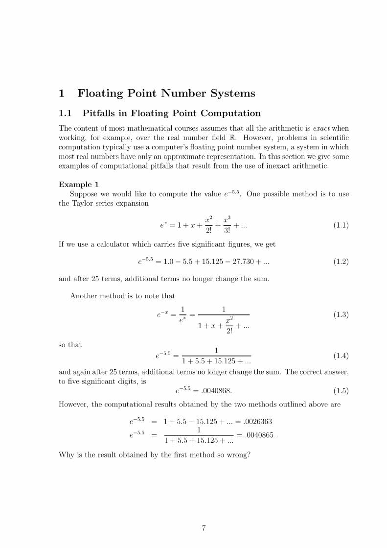
Example 1Suppose we would like to compute the value e−5.5. One possible method is to use
the Taylor series expansion
ex = 1 + x +x2
2!+
x3
3!+ ... (1.1)
If we use a calculator which carries five significant figures, we get
e−5.5 = 1.0− 5.5 + 15.125− 27.730 + ... (1.2)
and after 25 terms, additional terms no longer change the sum.
Another method is to note that
e−x =1
ex =1
1 + x +x2
2!+ ...
(1.3)
so that
e−5.5 =1
1 + 5.5 + 15.125 + ...(1.4)
and again after 25 terms, additional terms no longer change the sum. The correct answer,to five significant digits, is
e−5.5 = .0040868. (1.5)
However, the computational results obtained by the two methods outlined above are
e−5.5 = 1 + 5.5− 15.125 + ... = .0026363
e−5.5 =1
1 + 5.5 + 15.125 + ...= .0040865 .
Why is the result obtained by the first method so wrong?
7
1.2 Floating Point Numbers
For most of our discussions of numerical computation, we assume we are using thearithmetic of the mathematically defined real number system, which we denote by R.The number system R is infinite in two senses:
1. R is infinite in extent, in the sense that there are numbers, x, in R such that |x| isarbitrarily large.
2. R is infinite in density, in the sense that any interval I = {x | a ≤ x ≤ b} of R isan infinite set.
Digital computers can represent only finite sets of numbers, so all implementations ofalgorithms must use approximations to R and inexact arithmetic. The approximationsto R used by digital computers are known as floating point number systems.
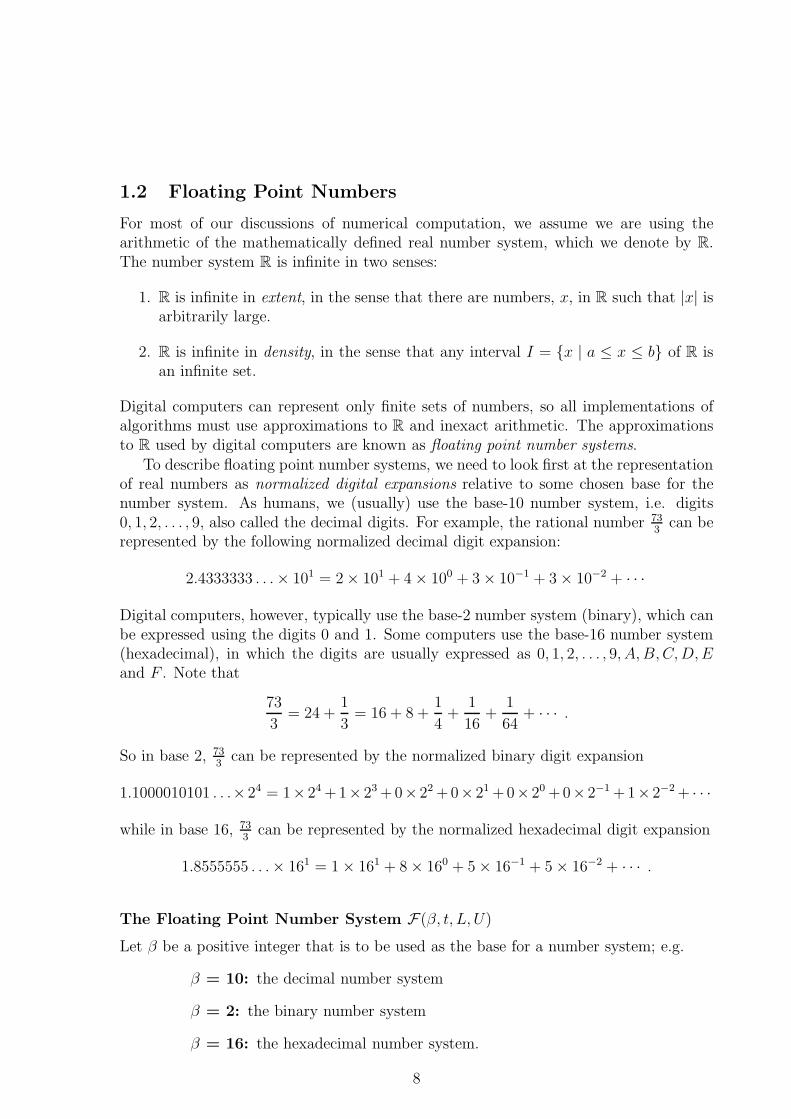
To describe floating point number systems, we need to look first at the representationof real numbers as normalized digital expansions relative to some chosen base for thenumber system. As humans, we (usually) use the base-10 number system, i.e. digits0, 1, 2, . . . , 9, also called the decimal digits. For example, the rational number 73
3can be
represented by the following normalized decimal digit expansion:
2.4333333 . . .× 101 = 2× 101 + 4× 100 + 3× 10⁻¹ + 3× 10⁻² + · · ·
Digital computers, however, typically use the base-2 number system (binary), which canbe expressed using the digits 0 and 1. Some computers use the base-16 number system(hexadecimal), in which the digits are usually expressed as 0, 1, 2, . . . , 9, A, B, C, D, Eand F . Note that
73
3= 24 +
1
3= 16 + 8 +
1
4+
1
16+
1
64+ · · · .
So in base 2, 733
can be represented by the normalized binary digit expansion
1.1000010101 . . .×24 = 1×24 +1×23 +0×22 +0×21 +0×20 +0×2−1 +1×2−2 + · · ·
while in base 16, 733
can be represented by the normalized hexadecimal digit expansion
1.8555555 . . .× 161 = 1× 161 + 8× 160 + 5× 16−1 + 5× 16−2 + · · · .
The Floating Point Number System F(β, t, L, U)
Let β be a positive integer that is to be used as the base for a number system; e.g.
β = 10: the decimal number system
β = 2: the binary number system
β = 16: the hexadecimal number system.
8
Any positive number in R can be represented by an infinite base-β expansion in thenormalized form
d0.d1d2d3 · · · × βp
where
- dk are base-β digits, i.e. dk ∈ {0, 1, . . . , β − 1}
- ‘normalized’ means d0 6= 0
- p is an integer (not necessarily positive).
We call d0.d1d2d3 . . . the significand (also sometimes called the mantissa), β the base,and p the exponent.
Floating point number systems limit the infinite density of R by retaining a fixednumber, t, of digits in the significand (t is called the precision of the number system).They limit the infinite extent of R by allowing only a finite number of integer values forthe exponent p, specifically by imposing the restriction L ≤ p ≤ U for two fixed integerbounds L and U . So every floating point number system is identified by four integerparameters, {β, t, L, U}, which are the base, the precision, and lower and upper boundson the exponent range. The numbers which can be represented in such a system areprecisely those of the form
± d0.d1d2...dt−1 × βp for L ≤ p ≤ U with d0 6= 0
and 0 (a special case).
There are two standardized floating point number systems that are widely used inthe design of computer software and hardware:
IEEE single precision system: {β = 2; t = 24; L = −126; U = 127}.IEEE double precision system: {β = 2; t = 53; L = −1022; U = 1023}.
We will denote a floating point number system by F(β, t, L, U) or sometimes simply byF when the parameters are understood.
1.3 Absolute and Relative Error
When we obtain a computed result, x, and we wish to discuss its relationship with thecorrect mathematical result, xexact, we can measure either the absolute error :
Errabs = |xexact − x|
or we can measure the relative error:
Errrel =|xexact − x||xexact|
.
Note: When measuring relative error, sometimes the value used in the denominator isthe computed value |x| rather than |xexact| as stated above. In most cases, the differencebetween the two definitions is insignificant.
9
For the type of computations performed on a digital computer, the relative errormeasure is most useful. This is because there is a close relationship between relativeerror and the number of correct significant digits in the computed result.Remark: The significant digits of a number are all the digits starting with the leftmostnonzero digit.
The computed result x is said to approximate xexact to about s significant digits if therelative error is approximately 10−s; or, to be more precise, if the relative error satisfies
0.5× 10−s ≤ |xexact − x||xexact|
< 5.0× 10−s . (1.6)
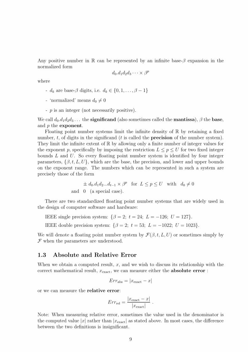
Consider the situation from Example 1. Two different methods are used to computea floating point approximation for the value e−5.5. The correct value, to five significantdigits, is
e−5.5 = 0.0040868 .
The value computed by the first method is x1 = 0.0026363, yielding a relative error of
Errrel =|0.0040868− x1|
0.0040868≈ 3.5× 10⁻¹ .
Based on equation (1.6), we would estimate that x1 has approximately one significantdigit correct (in actual fact, we can see that it has no correct digits).
Next consider the value computed by the second method, x2 = 0.0040865. Its relativeerror is
Errrel =|0.0040868− x2|
0.0040868≈ 0.7× 10⁻⁴ .
Based on equation (1.6), we would estimate that x2 has approximately four significantdigits correct. We can see that x2 is indeed correct to four significant digits.
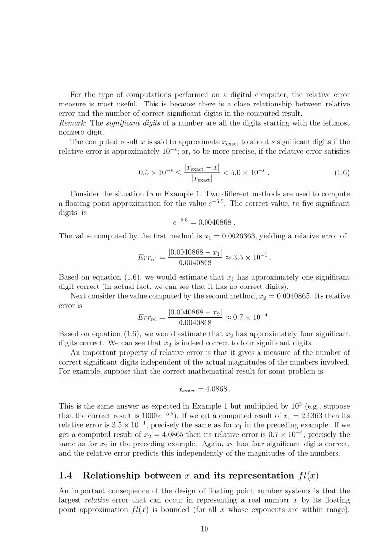
An important property of relative error is that it gives a measure of the number ofcorrect significant digits independent of the actual magnitudes of the numbers involved.For example, suppose that the correct mathematical result for some problem is
xexact = 4.0868 .
This is the same answer as expected in Example 1 but multiplied by 103 (e.g., supposethat the correct result is 1000 e−5.5). If we get a computed result of x1 = 2.6363 then itsrelative error is 3.5× 10⁻¹, precisely the same as for x1 in the preceding example. If weget a computed result of x2 = 4.0865 then its relative error is 0.7× 10⁻⁴, precisely thesame as for x2 in the preceding example. Again, x2 has four significant digits correct,and the relative error predicts this independently of the magnitudes of the numbers.
1.4 Relationship between x and its representation fl(x)
An important consequence of the design of floating point number systems is that thelargest relative error that can occur in representing a real number x by its floatingpoint approximation fl(x) is bounded (for all x whose exponents are within range).
10
This maximum relative error measure of machine precision is called machine epsilon,denoted here by ε. It is also called the unit roundoff error since ε can be defined asthe smallest representable number such that, in F(β, t, L, U),
1 + ε > 1 .
If a computer uses base β arithmetic with t digits in the significand, i.e. F(β, t, L, U),then the value of machine epsilon (or unit roundoff error) is
ε =1
2β1−t .
In general then, the relative error between any nonzero real number x and its floatingpoint representation is bounded by ε. Let fl(x) be the floating point representation ofx. Then
|fl(x)− x||x| ≤ ε .
This relationship can also be expressed as
fl(x)− x = δ x
where |δ| ≤ ε
and thus we have
fl(x) = x (1 + δ) (1.7)
where δ is some value (positive, negative or zero) such that −ε ≤ δ ≤ ε .
The IEEE standard basically says that a single arithmetic operation in F must bedone so that the computed result is rounded to the nearest representable floating pointnumber to the exact real arithmetic result. An exception occurs if the exponent isout of range, which leads to a state called overflow if the exponent is too large, orunderflow if the exponent is too small.
Let us denote the floating point addition operator in F by ⊕. Then for adding twofloating point numbers w, z ∈ F , using (1.7), we have
w ⊕ z = fl(w + z) = (w + z)(1 + δ) .
Next we will consider adding three floating point numbers a, b, c ∈ F using the floatingpoint addition operation in F .
Exercise
Make up an example to show that the sum of three numbers in F , computed using ⊕,depends on the order in which the terms are added. I.e. find values of a, b, c ∈ F suchthat
(a⊕ b)⊕ c 6= a⊕ (b⊕ c) .
11
1.5 Roundoff Error Analysis
Although each floating point arithmetic operation is done with a relative error that isbounded by ε, it is not the case that the result of a sequence of two or more floatingpoint arithmetic operations has a relative error that is bounded by ε. Consider addingthree floating point numbers a, b, c ∈ F .
How does (a ⊕ b) ⊕ c differ from the true sum a + b + c ? I.e., what is the size ofthe relative error in this sum computed in F? We will do a small exercise in traditionalfloating point error analysis to answer this question.
First we express (a⊕b)⊕c in terms of exact additions with relative error perturbationsδ1 due to the first operation, and δ2 due to the second operation:
(a⊕ b)⊕ c = (a + b)(1 + δ1)⊕ c =(
(a + b)(1 + δ1) + c)
(1 + δ2)
=(
(a + b + c) + (a + b)δ1
)
(1 + δ2)
= (a + b + c) + (a + b)δ1 + (a + b + c)δ2 + (a + b)δ1δ2 . (1.8)
Therefore,
|(a + b + c)− ((a⊕ b)⊕ c)| ≤ (|a|+ |b|+ |c|) (|δ1|+ |δ2|+ |δ1| |δ2|) (1.9)
where we have slightly increased the upper bound (the right hand side) to make thebound symmetric in the variables a, b and c. In other words, the upper bound as statedis not affected by the order of the terms in the sum.
If a + b + c 6= 0 then the relative error in the floating point sum
Errrel =|(a + b + c)− ((a⊕ b)⊕ c)|
|a + b + c|
is bounded as follows, from (1.9):
Errrel ≤|a|+ |b|+ |c||a + b + c| (2 ε + ε2) . (1.10)
Note that (1.10) tells us:
• if |a + b + c| ≈ |a|+ |b|+ |c| (for example, if a, b, c are all positive, or all negative)then Errrel is dominated by (2 ε + ε2) which is small;
• if |a + b + c| ≪ |a| + |b| + |c| then Errrel can be quite large, namely (2 ε + ε2)
multiplied by the “magnification factor” |a|+|b|+|c||a+b+c|
.
In what situations will the factor |a|+|b|+|c||a+b+c|
be very large? This will happen when
the denominator (the actual sum) is much smaller than the numerator (the sum of theabsolute values). This phenomenon, known as cancellation, can occur when adding amix of both positive and negative values.
For example, in the floating point number system F(10, 5,−10, 10), suppose that
a = 10000. , b = 3.1416 , c = −10000.
12
Then |a|+ |b|+ |c| = 20003.1416 and a + b + c = 3.1416. Thus, the relative error boundgiven by (1.10) is
Errrel ≤ 6367.2 (2 ε + ε2) ≈ 0.6
since ε = 1210−4. (Note that since the unit roundoff error ε is a small quantity, ε2 is very
small, and we can approximate 2 ε + ε2 ≈ 2 ε .) This relative error of 0.6× 100 is quitelarge, implying that there may be no significant digits correct in the result. Indeed, forthis example the computation proceeds as follows:
(a⊕ b)⊕ c = 10003.⊕ (−10000.) = 3.0000
compared with the true sum which is 3.1416 and therefore the computed sum actuallyhas one significant digit correct.
In contrast, using the same floating point number system F(10, 5,−10, 10), supposethat all three summands are positive:
a = 10000. , b = 3.1416 , c = 10000.
In this case the relative error bound given by (1.10) is
Errrel ≤ 2 ε + ε2 ≈ 2 ε ≈ 10−4
which implies that we can expect about four correct significant digits in the result. (Thisis a “best case” situation, where the relative error bound is a small multiple of ε.) Theactual computation for this case is as follows:
(a⊕ b)⊕ c = 10003.⊕ 10000. = 20003.
compared with the true sum which is 20003.1416 and we can see that we have, in fact,all five significant digits correct in this case.
The error bound (1.10) for the case of adding three numbers can be generalized tothe case of adding N numbers. Let xi ∈ F , i = 1, . . . , N , be N given floating pointnumbers (i.e. numbers stored in a computer system). If
fl
(
N∑
i=1
xi
)
denotes the computed result of adding the N numbers in F , and if∑N
i=1 xi 6= 0 thenthe relative error bound can be expressed as
∣
∣
∣
∑Ni=1 xi − fl
(
∑Ni=1 xi
)∣
∣
∣
∣
∣
∣
∑Ni=1 xi
∣
∣
∣
≤∑N
i=1 |xi|∣
∣
∣
∑Ni=1 xi
∣
∣
∣
1.01 N ε . (1.11)
The appearance of the factor 1.01 in (1.11) is an artificial technicality. We had notedin the roundoff error analysis for adding three numbers that, for practical purposes,
13
2 ε + ε2 ≈ 2 ε since ε is small. Similarly, the analysis leading to the bound (1.11) hasemployed a simplification such that an expression of the form
(N − 1) ε +(N − 1)(N − 2)
2ε2 + · · ·+ εN−1
has been replaced by an upper bound of the form 1.01 N ε, which holds as long asN < .01
ε. This level of detail is of no importance to us here; in applying the bound (1.11)
we understand that, for practical purposes, 1.01 N ε ≈ N ε .
A similar roundoff error analysis for a product of numbers, rather than a sum, showsthat the error bound is always approximately N ε . This arises because for a product wehave
∣
∣
∣
∣
∣
N∏
i=1
xi
∣
∣
∣
∣
∣
=
N∏
i=1
|xi|
and therefore,∣
∣
∣
∏Ni=1 xi − fl
(
∏Ni=1 xi
)∣
∣
∣
∣
∣
∣
∏Ni=1 xi
∣
∣
∣
≤ 1.01 N ε . (1.12)
1.6 Conditioning and Stability
It is important to understand the concept that some problems, as posed, may be well-conditioned and some may be ill-conditioned. More precisely, we like to have a measureof how well-conditioned (or how ill-conditioned) a given problem may be. The conceptof conditioning may be defined as follows.
Consider a problem P with input values I and output values O. If a small change ofsize ∆I in one or more input values causes a relatively small change in the mathematicallycorrect output values, then the problem is said to be well-conditioned. Otherwise, theproblem is said to be ill-conditioned. Stated another way, an ill-conditioned problemhas output that is very sensitive to slight changes in the input.
Remark 1: This phenomenon is a statement about a mathematical problem, and is notdue to floating point errors.
Remark 2: There is always a “sliding scale” for “how well-conditioned” or “how ill-conditioned” a particular problem is.
Example 2
Finding the point of intersection of two lines requires some calculation. Dependingon the lines themselves, this calculation may be well-conditioned or ill-conditioned. Thelines in Figure 1(a) are nearly perpendicular. A small adjustment to the slope of one ofthe lines will not move the point of intersection very much, and hence that calculationis well-conditioned. On the other hand, the lines in Figure 1(b) are nearly parallel. Aslight adjustment to the slope of one of those lines will move the point of intersectionquite a lot. That calculation is ill-conditioned.
14
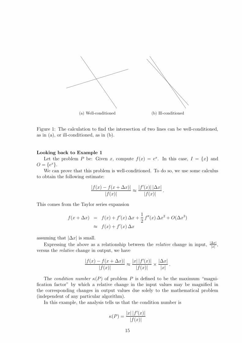
(a) Well-conditioned (b) Ill-conditioned
Figure 1: The calculation to find the intersection of two lines can be well-conditioned,as in (a), or ill-conditioned, as in (b).
Looking back to Example 1
Let the problem P be: Given x, compute f(x) = ex. In this case, I = {x} andO = {ex}.
We can prove that this problem is well-conditioned. To do so, we use some calculusto obtain the following estimate:
|f(x)− f(x + ∆x)||f(x)| ≈ |f
′(x)| |∆x||f(x)| .
This comes from the Taylor series expansion
f(x + ∆x) = f(x) + f ′(x) ∆x +1
2f ′′(x) ∆x2 + O(∆x3)
≈ f(x) + f ′(x) ∆x
assuming that |∆x| is small.
Expressing the above as a relationship between the relative change in input, |∆x||x|
,versus the relative change in output, we have
|f(x)− f(x + ∆x)||f(x)| ≈ |x| |f
′(x)||f(x)| ×
|∆x||x| .
The condition number κ(P ) of problem P is defined to be the maximum “magni-fication factor” by which a relative change in the input values may be magnified inthe corresponding changes in output values due solely to the mathematical problem(independent of any particular algorithm).
In this example, the analysis tells us that the condition number is
κ(P ) =|x| |f ′(x)||f(x)|
15
for any function f(x). In our example, f ′(x) = f(x) so in this particular case we have
κ(P ) = |x| .
The computational results obtained by the two methods outlined in Example 1 are
e−5.5 = 1− 5.5 + 15.125− · · · = 0.0026363
e−5.5 =1
1 + 5.5 + 15.125 + · · · = 0.0040865 .
Using a “bad algorithm” (the first method), the computed result was 0.0026363 com-pared with the correct value which is 0.0040868. In other words, all digits in the com-puted result are wrong!
This bad computational result cannot be blamed on the problem: the problem asstated is well-conditioned. From above, the condition number for this problem is
κ(P ) = |x| = 5.5 .
Noting that κ(P ) < 10, we can conclude that roundoff errors (in relative error) of size ε(the unit roundoff error) can lead to relative errors in the output bounded by
Errrel ≈ κ(P ) ε < 10 ε .
For example, if ε is approximately 10−5 as in Example 1, then the output might haverelative error as large as 10−4 meaning that we should expect to have about four signif-icant digits correct (rather than than all five digits correct). This is the worst that canhappen due to the conditioning of the problem.
Any larger errors, such as seen in this example, must be blamed on the choice ofa bad algorithm. Indeed, Example 1 shows a good algorithm which computes e−5.5 togood accuracy. We say that the first computation is using an unstable algorithm andthe second computation is using a stable algorithm. The concept of stability may bedefined as follows in a general setting.
Consider a problem P with condition number κ(P ) and suppose that we apply al-gorithm A to solve problem P . If we can guarantee that the computed output valuesfrom algorithm A will have relative errors not too much larger than the errors due tothe condition number κ(P ), then algorithm A is said to be stable. Otherwise, if thecomputed output values from algorithm A can have much larger relative errors, thenalgorithm A is said to be unstable.
We can state the concept of stability more informally as follows. If an algorithmproduces inaccurate results, we have to try to determine whether the errors can beblamed on the mathematical problem as stated (i.e. the problem has a large conditionnumber), or, as is often the case, we have chosen an unstable algorithm to solve theproblem. In the latter case, we try to find a more stable algorithm; i.e., an algorithmwhich does not cause a large magnification of errors. Since we always commit roundofferrors during the execution of an algorithm in a floating point number system, it is themagnification of such errors that is of concern to us.
16
Exercises
1. The numbers in a floating point system F(β, t, L, U) are defined by a base β, asignificand length t, and an exponent range [L, U ]. A nonzero floating point numberx has the form
x = ± d0.d1d2 · · · dt−1 × βe .
Here d0.d1d2 · · · dt−1 is the significand and e is the exponent. The exponent satisfiesL ≤ e ≤ U . The di are base-β digits and satisfy 0 ≤ di ≤ β−1. Nonzero floating pointnumbers x are normalized: d0 6= 0. The floating point number zero is represented bysetting all digits in the significand to zero and setting e = L.
(a) What is the largest value of n so that n! can be exactly represented in the floatingpoint number system F(2, 5,−10, 10)? Show your work.
(b) Suppose that on a base-2 computer, the distance between 7 and the next largestfloating point number is 2−12. What is the distance between 70 and the nextlargest floating point number?
(c) Assume that x and y are normalized positive floating point numbers in a base-2computer with t-bit significand. How small can y − x be if x < 8 < y?
2. Consider a fictitious floating point number system composed of the following num-bers:
S = { ± d1.d2d3 × 2±y : d2, d3, y = 0 or 1,
and d1 = 1 unless d1 = d2 = d3 = 0 } .
I.e. each number is normalized unless it is the number zero.
(a) Plot the elements of S on the real axis.
(b) Indicate on your plot the regions of OFL (overflow) and UFL (underflow).
(c) How many elements are contained in S?
(d) What is the value of ε (machine epsilon)?
3. Using the floating point number system F(2, 20,−200, 200), represent the distancebetween the Earth and the Sun (1.5 × 10⁸ kilometers) and the distance betweenToronto and Waterloo (110 kilometers). What length does the last bit of the signifi-cand represent in each case?
4. Carry out a roundoff error analysis to show that, in a floating point number system,if ab + c 6= 0 then
|(ab + c)− ((a⊗ b)⊕ c)||ab + c| ≤ |ab|
|ab + c|ε (1 + ε) + ε
where ε denotes machine epsilon. Justify each inequality that you introduce.
17

18
2 Interpolation
It is often the case that one has a discrete (finite) set of data (x1, y1), . . . , (xn, yn) thatdescribes the behaviour of some (unknown) function g(x) and that one wishes to deter-mine g(x) or at least some approximation to g(x). One can then use this function toevaluate the data at some unknown values, determine instantaneous changes at somepoints (i.e., estimate the derivative), and so on.
One approach is to require that our approximate function g(x) should have theproperty that it interpolates the data, that is,
g(x1) = y1, . . . , g(xn) = yn. (2.1)
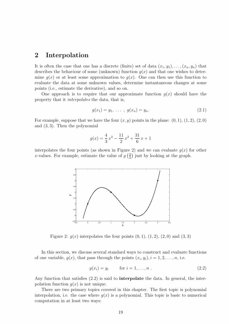
For example, suppose that we have the four (x, y) points in the plane: (0, 1), (1, 2), (2, 0)and (3, 3). Then the polynomial
g(x) =4
3x3 − 11
2x2 +
31
6x + 1
interpolates the four points (as shown in Figure 2) and we can evaluate g(x) for otherx-values. For example, estimate the value of g
(
32
)
just by looking at the graph.
−0.5 0 0.5 1 1.5 2 2.5 3 3.5−0.5
0
0.5
1
1.5
2
2.5
3
3.5
4
x
y
Figure 2: g(x) interpolates the four points (0, 1), (1, 2), (2, 0) and (3, 3)
In this section, we discuss several standard ways to construct and evaluate functionsof one variable, g(x), that pass through the points (xi, yi), i = 1, 2, . . . , n, i.e.
g(xi) = yi for i = 1, . . . , n . (2.2)
Any function that satisfies (2.2) is said to interpolate the data. In general, the inter-polation function g(x) is not unique.
There are two primary topics covered in this chapter. The first topic is polynomialinterpolation, i.e. the case where g(x) is a polynomial. This topic is basic to numericalcomputation in at least two ways:
19
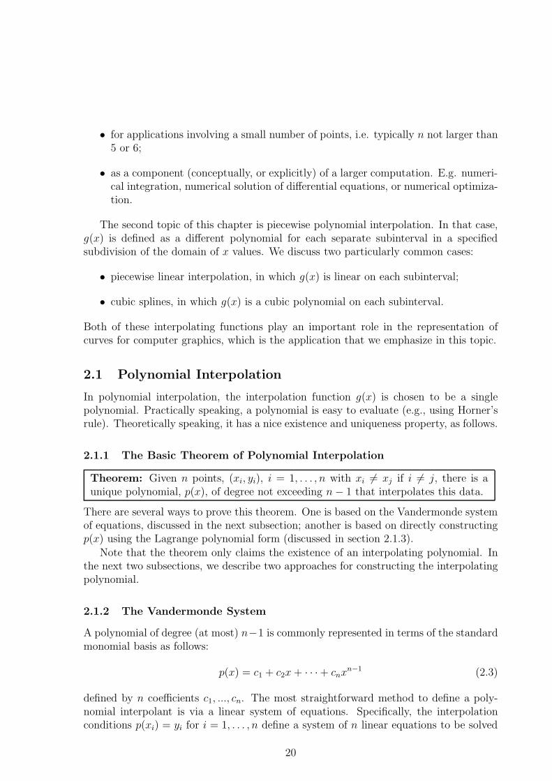
• for applications involving a small number of points, i.e. typically n not larger than5 or 6;
• as a component (conceptually, or explicitly) of a larger computation. E.g. numeri-cal integration, numerical solution of differential equations, or numerical optimiza-tion.
The second topic of this chapter is piecewise polynomial interpolation. In that case,g(x) is defined as a different polynomial for each separate subinterval in a specifiedsubdivision of the domain of x values. We discuss two particularly common cases:
• piecewise linear interpolation, in which g(x) is linear on each subinterval;
• cubic splines, in which g(x) is a cubic polynomial on each subinterval.
Both of these interpolating functions play an important role in the representation ofcurves for computer graphics, which is the application that we emphasize in this topic.
2.1 Polynomial Interpolation
In polynomial interpolation, the interpolation function g(x) is chosen to be a singlepolynomial. Practically speaking, a polynomial is easy to evaluate (e.g., using Horner’srule). Theoretically speaking, it has a nice existence and uniqueness property, as follows.
2.1.1 The Basic Theorem of Polynomial Interpolation
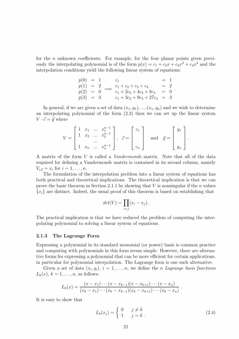
Theorem: Given n points, (xi, yi), i = 1, . . . , n with xi 6= xj if i 6= j, there is aunique polynomial, p(x), of degree not exceeding n− 1 that interpolates this data.
There are several ways to prove this theorem. One is based on the Vandermonde systemof equations, discussed in the next subsection; another is based on directly constructingp(x) using the Lagrange polynomial form (discussed in section 2.1.3).
Note that the theorem only claims the existence of an interpolating polynomial. Inthe next two subsections, we describe two approaches for constructing the interpolatingpolynomial.
2.1.2 The Vandermonde System
A polynomial of degree (at most) n−1 is commonly represented in terms of the standardmonomial basis as follows:
p(x) = c1 + c2x + · · ·+ cnxn−1 (2.3)
defined by n coefficients c1, ..., cn. The most straightforward method to define a poly-nomial interpolant is via a linear system of equations. Specifically, the interpolationconditions p(xi) = yi for i = 1, . . . , n define a system of n linear equations to be solved
20
for the n unknown coefficients. For example, for the four planar points given previ-ously the interpolating polynomial is of the form p(x) = c1 + c2x + c3x
2 + c4x3 and the
interpolation conditions yield the following linear system of equations:
p(0) = 1p(1) = 2p(2) = 0p(3) = 3
=⇒c1 = 1c1 + c2 + c3 + c4 = 2c1 + 2c2 + 4c3 + 8c4 = 0c1 + 3c2 + 9c3 + 27c4 = 3
.
In general, if we are given a set of data (x1, y1), ..., (xn, yn) and we wish to determinean interpolating polynomial of the form (2.3) then we can set up the linear systemV · ~c = ~y where
V =
1 x1 ... xn−11
1 x2 ... xn−12
...1 xn ... xn−1
n
, ~c =
c1
cn
and ~y =
y1
yn
.
A matrix of the form V is called a Vandermonde matrix. Note that all of the datarequired for defining a Vandermonde matrix is contained in its second column, namelyVi,2 = xi for i = 1, . . . , n.
The formulation of the interpolation problem into a linear system of equations hasboth practical and theoretical implications. The theoretical implication is that we canprove the basic theorem in Section 2.1.1 by showing that V is nonsingular if the n values{xi} are distinct. Indeed, the usual proof of this theorem is based on establishing that
det(V ) =∏
i<j
(xi − xj).
The practical implication is that we have reduced the problem of computing the inter-polating polynomial to solving a linear system of equations.
2.1.3 The Lagrange Form
Expressing a polynomial in its standard monomial (or power) basis is common practiceand computing with polynomials in this form seems simple. However, there are alterna-tive forms for expressing a polynomial that can be more efficient for certain applications,in particular for polynomial interpolation. The Lagrange form is one such alternative.
Given a set of data (xi, yi), i = 1, . . . , n, we define the n Lagrange basis functionsLk(x), k = 1, . . . , n, as follows:
Lk(x) =(x− x1) · · · (x− xk−1)(x− xk+1) · · · (x− xn)
(xk − x1) · · · (xk − xk−1)(xk − xk+1) · · · (xk − xn).
It is easy to show that
Lk(xj) =
{
0 j 6= k1 j = k .
(2.4)
21
Note that Lk(x), for any other real number x, need not be 0 or 1.Define a polynomial p(x) in terms of the Lagrange basis functions using as coefficients
the given {yi} data values as follows:
p(x) = y1L1(x) + y2L2(x) + · · ·+ ynLn(x) .
Then p(x) is a polynomial of degree n − 1 that interpolates the n data points since foreach i we have
p(xi) = y1L1(xi) + · · ·+ yiLi(xi) + · · ·+ ynLn(xi)= y1 · 0 + · · ·+ yi · 1 + · · ·+ yn · 0= yi .
For the cubic example (interpolating four points) discussed above, we have:
L1(x) = (x−1)(x−2)(x−3)(−1)(−2)(−3)
= (x−1)(x−2)(x−3)−6
L2(x) = (x−0)(x−2)(x−3)(1)(−1)(−2)
= (x)(x−2)(x−3)2
L3(x) = (x−0)(x−1)(x−3)(2)(1)(−1)
= (x)(x−1)(x−3)−2
L4(x) = (x−0)(x−1)(x−2)(3)(2)(1)
= (x)(x−1)(x−2)6
and the Lagrange interpolating polynomial is
p(x) = 1 · L1(x) + 2 · L2(x) + 0 · L3(x) + 3 · L4(x)= −1
6(x− 1)(x− 2)(x− 3) + x(x− 2)(x− 3) + 1
2x(x− 1)(x− 2) .
One can check by multiplying out the factors that the polynomial expressed here inLagrange form is the same polynomial determined previously in standard monomialform, namely
p(x) =4
3x3 − 11
2x2 +
31
6x + 1 .
Exercises
1. Consider data (x1, y1), (x2, y2), (x3, y3) with x1 < x2 < x3 and y2 > max(y1, y3).Graphically, the middle data point is higher than the two end points. This data isinterpolated by a quadratic polynomial, p2(x). Intuitively, it seems clear that p2(x)lies above the line joining the two end data points for x1 < x < x3, and, consequently,there is a maximum value of p2(x) in this interval.
We want to show algebraically that this is correct and give a formula for the max-imum. The algebra (and programs for doing computations) are simplified by doingsome transformations of the data. By rescaling the x-variable, we can assume thatx1 = 0 and x3 = 1; we will rename x2 = a for convenience. Without loss of generality,we can also assume that y1 < y3 and, by subtracting y1 from each yk, that y1 = 0.
(a) The line interpolating the end points of the normalized data is p1(x) = y3x.Show that p2(x) > p1(x) for 0 < x < 1.Hint: The Lagrange representation of p2(x) may be helpful.
22
(b) Show that the coefficient of x2 in p2(x) is negative.
(c) Let xmax be the x-value at which p2(x) achieves its maximum. Derive a formulafor xmax in terms of a, y2, and y3.
2. Let Lk(x), k = 1 . . . n, be the Lagrange basis functions for xk = k, k = 1 . . . n. Byconsidering an appropriately chosen data set {yk} and using the basic theorem inSection 2.1.1, prove that
n∑
k=1
k Lk(x) = x
for every value of x.
2.2 Piecewise Polynomial Interpolation
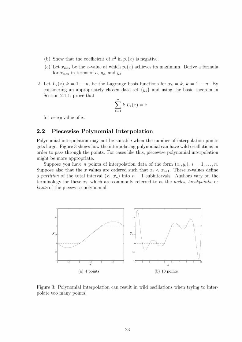
Polynomial interpolation may not be suitable when the number of interpolation pointsgets large. Figure 3 shows how the interpolating polynomial can have wild oscillations inorder to pass through the points. For cases like this, piecewise polynomial interpolationmight be more appropriate.
Suppose you have n points of interpolation data of the form (xi, yi), i = 1, . . . , n.Suppose also that the x values are ordered such that xi < xi+1. These x-values definea partition of the total interval (x1, xn) into n − 1 subintervals. Authors vary on theterminology for these xi, which are commonly referred to as the nodes, breakpoints, orknots of the piecewise polynomial.
1 1.5 2 2.5 3 3.5 4−1
−0.5
0
0.5
1
1.5
2
x
y
(a) 4 points
1 2 3 4 5 6 7 8 9 10−1
−0.5
0
0.5
1
1.5
2
x
y
(b) 10 points
Figure 3: Polynomial interpolation can result in wild oscillations when trying to inter-polate too many points.
23
A piecewise polynomial interpolant, s(x), is:
• a function of x for x1 ≤ x ≤ xn,
• an interpolant, i.e. s(xi) = yi,
• a polynomial for each subinterval, (xi, xi+1), usually different oneach subinterval,
• continuous for the total interval [x1, xn].
(2.5)
The Matlab command plot(x,y), for vector arguments x and y, creates a plot of thepiecewise-linear (degree 1) interpolant of (xi, yi), i = 1, . . . , n.
2.2.1 Cubic Spline Interpolants
This is a case in which the polynomial on each subinterval is of degree (at most) 3. LetS(x) be a cubic spline with knots at xi. Some of the defining characteristics of S(x) are:
1. S(x) is a piecewise polynomial interpolant (see (2.5));
2. S(x) is of degree ≤ 3 between the knots; i.e., it is a cubic polynomial on eachsubinterval;
3. S(x) is twice continuously differentiable; i.e.,
dS(x)
dxand
d2S(x)
dx2
are continuous functions for x1 ≤ x ≤ xn.
It would be nice if these three conditions completely defined S(x). But, unfortunately,they do not. It is necessary to add additional requirements at the end points, x1 and xn,to completely define S(x). Different applications of cubic splines will call for differentchoices for these end conditions, and this brings some messy technicalities to the dis-cussion of cubic splines. For good results in applications (e.g., graphics), it is importantthat these details be addressed correctly.
Computing with a cubic spline, S(x), involves two activities:
• computing a representation for S(x) from the data (xi, yi);
• evaluating S(x) at one (or more) values of x, i.e., evaluating S(x) using the chosenrepresentation.
2.2.2 Matlab Support for Splines
Matlab’s support for interpolation computations in one variable can be thought of asbeing organized into three layers of increasing technical detail and complexity of use.The simpler layers use the more complex ones and hide their details from the user. It isreasonable to refer to these as ‘layers’ because these names are overloaded; the function
24
that they perform depends on the form of parameter sequence, i.e. the signature of thecommand. This can be seen from the help <cmd> documentation for each.
The Matlab command interp1 is the simplest, least specific layer. The primarycommand of the second layer is the spline command. Using different signatures, splinecan be used to either
(a) combine the two tasks of computing the representation and evaluating S at pre-scribed arguments, or
(b) just compute the representation.
If the vectors x and y hold the interpolation data (i.e. the x- and y-coordinates of theinterpolation points), and xeval holds the x-values at which one wants to evaluate thecubic spline, then task (a) is accomplished by the Matlab command
yeval = spline(x,y,xeval) .
The vector yeval contains the corresponding values of S(x).Matlab calls its internal representation of a cubic spline a ppform. If Matlab’s spline
command is called as
pp = spline(x,y)
then the ppform is returned in variable ‘pp’. This variable is not useful directly, butcan be passed to Matlab command ppval, along with an argument vector at which youwant to evaluate the spline, in order to get the corresponding vector of spline values.
The most complex layer is formed by the spline toolbox of Matlab. This layer hasmany commands which can be listed by entering help splines. For example, csape isa more sophisticated function to compute cubic splines.
2.2.3 Representation of S(x)
There are two basic concepts associated with the representation of cubic splines that wehope to convey. One is that continuity of S(x) and its derivatives across a breakpointxk places conditions on the coefficients of the representations in the adjoining intervals[xk−1, xk] and [xk, xk+1]. This is, of course, common to piecewise polynomial represen-tation generally. The second concept is that for cubic splines these conditions lead to asystem of linear equations in which the coefficients of the cubic spline representation arethe unknowns. This system must be solved to find values for these coefficients. Fortu-nately, the system of equations has a special form (tridiagonal), enabling it to be solvedvery efficiently. Otherwise, cubic splines would be less practical.
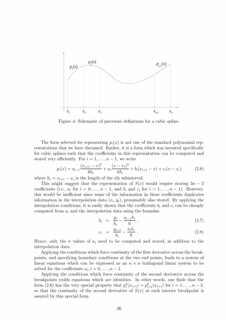
A standard representation for a cubic spline is based on defining S(x) as a cubicpolynomial pi(x) on each subinterval xi ≤ x ≤ xi+1. Figure 4 presents a schematic ofthe definition.
25
x2 x3 xn-1 xn
p (x)2
n-1p (x)
x1
p (x)1
Figure 4: Schematic of piecewise definitions for a cubic spline.
The form selected for representing pi(x) is not one of the standard polynomial rep-resentations that we have discussed. Rather, it is a form which was invented specificallyfor cubic splines such that the coefficients in this representation can be computed andstored very efficiently. For i = 1, . . . , n− 1, we write
pi(x) = ai−1(xi+1 − x)3
6hi
+ ai(x− xi)
3
6hi
+ bi(xi+1 − x) + ci(x− xi) (2.6)
where hi = xi+1 − xi is the length of the ith subinterval.This might suggest that the representation of S(x) would require storing 3n − 2
coefficients (i.e., ai for i = 0, . . . , n − 1, and bi and ci for i = 1, . . . , n − 1). However,this would be inefficient since some of the information in these coefficients duplicatesinformation in the interpolation data (xi, yi), presumably also stored. By applying theinterpolation conditions, it is easily shown that the coefficients bi and ci can be cheaplycomputed from ai and the interpolation data using the formulas
bi =yi
hi− ai−1hi
6, (2.7)
ci =yi+1
hi− aihi
6. (2.8)
Hence, only the n values of ai need to be computed and stored, in addition to theinterpolation data.
Applying the conditions which force continuity of the first derivative across the break-points, and specifying boundary conditions at the two end points, leads to a system oflinear equations which can be expressed as an n × n tridiagonal linear system to besolved for the coefficients ai, i = 0, . . . , n− 1.
Applying the conditions which force continuity of the second derivative across thebreakpoints yields equations which are identities. In other words, one finds that theform (2.6) has the very special property that p′′i (xi+1) = p′′i+1(xi+1) for i = 1, . . . , n− 2,so that the continuity of the second derivative of S(x) at each interior breakpoint isassured by this special form.
26
Exercises
1. (a) Show that p′′i (xi+1) = ai. Why is this not sufficient to ensure that S(x) is twicecontinuously differentiable?
(b) The requirement that S(x) be continuous means that
limx→xi−
S(x) = limx→xi+
S(x) (2.9)
at each internal knot, i.e. for i = 2, . . . , n − 1. “limx→xi− S(x)” is the limit ofthe values of S(x) as x → xi while x < xi; it is called the limit from the left.Clearly, limx→xi− S(x) = limx→xi− pi−1(x), since if x is near xi but x < xi thenx is in the (i− 1)st subinterval.Show that the continuity condition, (2.9) and the interpolation condition forS(x) at x = xi require
limx→xi−
pi−1(x) = yi (2.10)
limx→xi+
pi(x) = yi . (2.11)
(c) Show that (2.10) implies (2.8) and that (2.11) implies (2.7).
2. Consider the following alternative representation for a cubic spline, S(x):
S(x) =
a + b(x− 1) + c(x− 1)2 − 14(x− 1)2(x− 2) 1 ≤ x ≤ 2
e + f(x− 2) + g(x− 2)2 + 14(x− 2)2(x− 3) 2 ≤ x ≤ 3.
We also wish our cubic spline to satisfy the boundary conditions:
d2S
dx2(1) = 0 ,
d2S
dx2(3) = 0 .
(a) What are the conditions on the coefficients a through g such that S(x) interpo-lates the points (1,1), (2,1), and (3,0)? Deduce the values of a and e.
(b) What is the condition on the coefficients such that S ′(x) is continuous at x = 2?
(c) Show that enforcing the boundary conditions at x = 1 and x = 3 leads to c = −14
and g = −12.
(d) Compute the values of b and f from part (a).
(e) To ensure that S(x) is a cubic spline, what other condition needs to be checked?(It is not necessary to actually verify this condition for the purpose of thisexercise.)
27

28
3 Planar Parametric Curves
3.1 Introduction to Parametric Curves
This is a short introduction to concepts, examples, and terminology of parametric curvesin the x-y plane. Parametric curves are directed curves described by a pair of continuousfunctions, x(t) and y(t), of a common argument t usually called the parameter, for
a ≤ t ≤ b. For notational convenience, we define the vector function ~P (t) = (x(t), y(t)).
The curve C is the set of points {~P (t) | a ≤ t ≤ b}.
Some Examples
C1: x(t) = cos(πt), y(t) = sin(πt), 0 ≤ t ≤ 1 .
C1 is the semi-circle in the upper half plane directed from (1, 0) to (−1, 0).
C2: x(t) = cos(π(1− t)), y(t) = sin(π(1− t)), 0 ≤ t ≤ 1 .
C2 is C1 with its direction reversed.
C3: x(t) = cos(πt2), y(t) = sin(πt2), 0 ≤ t ≤ 1 .
C3 is visually the same curve as C1, but it has a different parameterization. Math-ematically, it is a different parametric curve.
C4: x(t) = cos(πt), y(t) = sin(πt), 0 ≤ t ≤ 2 .
C4 is the entire circle; it is a closed curve, whereas the previous examples are opencurves. It is a simple curve, meaning that it does not intersect itself.
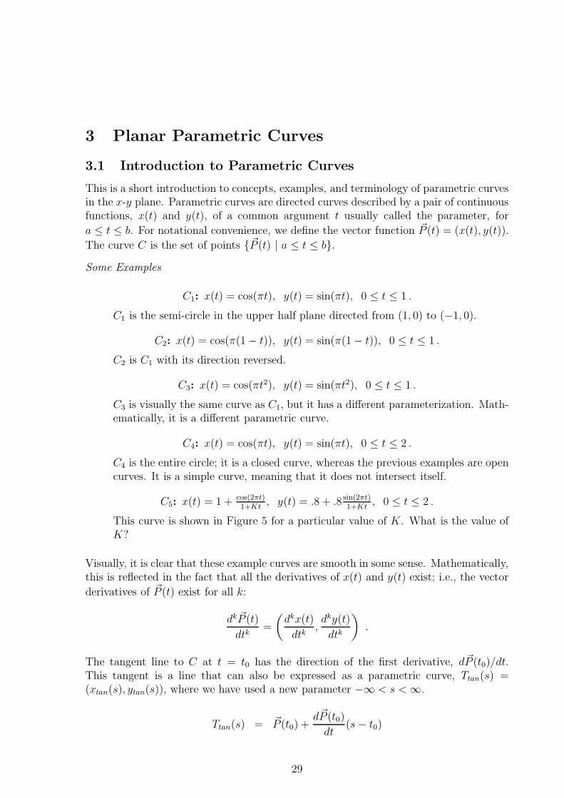
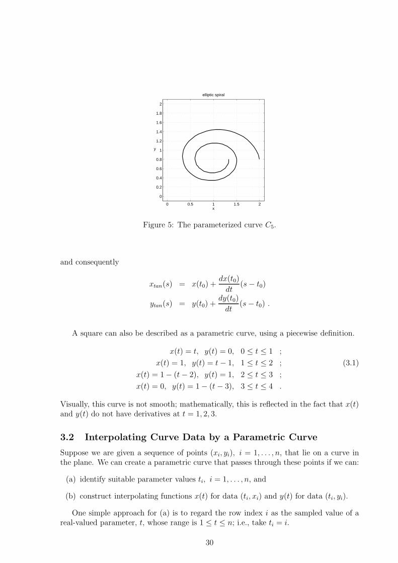
C5: x(t) = 1 + cos(2πt)1+Kt
, y(t) = .8 + .8 sin(2πt)1+Kt
, 0 ≤ t ≤ 2 .
This curve is shown in Figure 5 for a particular value of K. What is the value ofK?
Visually, it is clear that these example curves are smooth in some sense. Mathematically,this is reflected in the fact that all the derivatives of x(t) and y(t) exist; i.e., the vector
derivatives of ~P (t) exist for all k:
dk ~P (t)
dtk=
(
dkx(t)
dtk,dky(t)
dtk
)
.
The tangent line to C at t = t0 has the direction of the first derivative, d~P (t0)/dt.This tangent is a line that can also be expressed as a parametric curve, Ttan(s) =(xtan(s), ytan(s)), where we have used a new parameter −∞ < s <∞.
Ttan(s) = ~P (t0) +d~P (t0)
dt(s− t0)
29
0 0.5 1 1.5 2
0
0.2
0.4
0.6
0.8
1
1.2
1.4
1.6
1.8
2
elliptic spiral
x
y
Figure 5: The parameterized curve C5.
and consequently
xtan(s) = x(t0) +dx(t0)
dt(s− t0)
ytan(s) = y(t0) +dy(t0)
dt(s− t0) .
A square can also be described as a parametric curve, using a piecewise definition.
x(t) = t, y(t) = 0, 0 ≤ t ≤ 1 ;
x(t) = 1, y(t) = t− 1, 1 ≤ t ≤ 2 ; (3.1)
x(t) = 1− (t− 2), y(t) = 1, 2 ≤ t ≤ 3 ;
x(t) = 0, y(t) = 1− (t− 3), 3 ≤ t ≤ 4 .
Visually, this curve is not smooth; mathematically, this is reflected in the fact that x(t)and y(t) do not have derivatives at t = 1, 2, 3.
3.2 Interpolating Curve Data by a Parametric Curve
Suppose we are given a sequence of points (xi, yi), i = 1, . . . , n, that lie on a curve inthe plane. We can create a parametric curve that passes through these points if we can:
(a) identify suitable parameter values ti, i = 1, . . . , n, and
(b) construct interpolating functions x(t) for data (ti, xi) and y(t) for data (ti, yi).
One simple approach for (a) is to regard the row index i as the sampled value of areal-valued parameter, t, whose range is 1 ≤ t ≤ n; i.e., take ti = i.
30
For step (b), we could use piecewise linear interpolation, giving a function xpl(t) for0 ≤ t ≤ n. If we did the same thing with the y coordinate data, we would get anotherfunction, ypl(t), for 0 ≤ t ≤ n, and together (xpl(t), ypl(t)) define a parametric curvepassing through the data points. By default, the Matlab plotting command plot(x,y)
plots the piecewise linear interpolation curve, (xpl(t), ypl(t)).For a smoother interpolating curve, consider using cubic spline interpolation. I.e.,
interpolate (ti, xi) by a cubic spline function, xcs(t), and do the same for the y coordinatedata. Then we would have a smooth interpolating parametric curve (xcs(t), ycs(t)).
How well would using a piecewise linear interpolating parametric curve work forrepresenting the unit square curve in equation (3.1)? How well would using a cubicspline interpolating parametric curve work for this same curve?
For cubic spline interpolation, choosing the parameter values ti = i can lead to acurve that does not look the way you intended due to distortions caused by this naivechoice of parameterization. An ideal parameterization would be one where the parametervalues ti reflect the arc length distance along the curve between successive data points.A good approximation to this ideal is obtained by defining successive parameter valuesti based on the Euclidean distance between points, namely
ti+1 = ti +√
(xi+1 − xi)2 + (yi+1 − yi)2 . (3.2)
3.3 Graphics for Handwriting
Handwriting can be viewed as a series of curve segments in the plane. Here we discusscreating a computer representation of handwriting based on interpolating parametriccurves using cubic splines. See Appendix A for an example and a discussion of cus-tomizing plots for different purposes.
Consider the following Matlab based procedure for representing a single script letter,or a word.
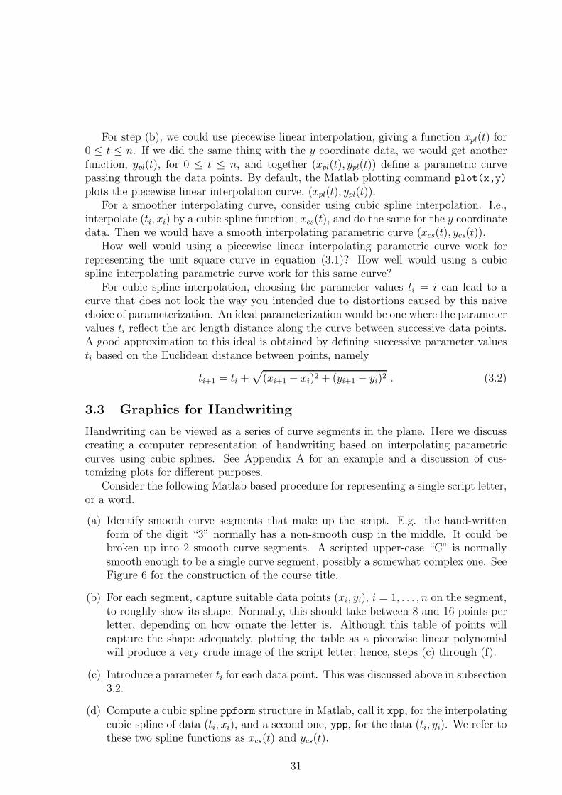
(a) Identify smooth curve segments that make up the script. E.g. the hand-writtenform of the digit “3” normally has a non-smooth cusp in the middle. It could bebroken up into 2 smooth curve segments. A scripted upper-case “C” is normallysmooth enough to be a single curve segment, possibly a somewhat complex one. SeeFigure 6 for the construction of the course title.
(b) For each segment, capture suitable data points (xi, yi), i = 1, . . . , n on the segment,to roughly show its shape. Normally, this should take between 8 and 16 points perletter, depending on how ornate the letter is. Although this table of points willcapture the shape adequately, plotting the table as a piecewise linear polynomialwill produce a very crude image of the script letter; hence, steps (c) through (f).
(c) Introduce a parameter ti for each data point. This was discussed above in subsection3.2.
(d) Compute a cubic spline ppform structure in Matlab, call it xpp, for the interpolatingcubic spline of data (ti, xi), and a second one, ypp, for the data (ti, yi). We refer tothese two spline functions as xcs(t) and ycs(t).
31
End Result Using Splines
−15 −10 −5 0 5 10 15 20 25 30 35 40−10
−5
0
5
10Curve and Point Data
x axis
y ax
is
Figure 6: Constructing the CS 370 logo with splines.
(e) Compute a finer partition, trefj of the parameter interval t1 ≤ t ≤ tn.
(f) Create plotting points (xrefi, yrefi) by evaluating the cubic splines at each param-eter value in trefj. i.e. xrefi = xcs(trefi) and yrefi = ycs(trefi) for i = 1, . . . , n.Finally, plot (xrefi, yrefi).
This process has been followed to produce the CS 370 logo that appears on the titlepage of these notes. In Figure 6, we show the result of steps (a) and (b) in the lowerfigure, and the result of steps (e) and (f), plotted with no axes, in the upper figure.
Some details
Steps (a) and (b)A simple way to accomplish steps (a) and (b) is to write a large version of the letter(or word) on squared graph paper. Identify the segments and mark the data pointson the curve segments. Introduce an x axis and a y axis on the paper and read offthe coordinates of the sequence of points on each segment. For efficiency, pick a smallnumber of data points to capture the main features of the shape. If the curve segmentis closed (e.g. the letter “O”), repeat the first data point as the last one in the sequence.
Step (d)Some spline end conditions work better than others, depending on the curve and its
32
position in the letter. In general, this can only be determined by trial and error; however,for smooth closed curves, periodic end conditions should be used.
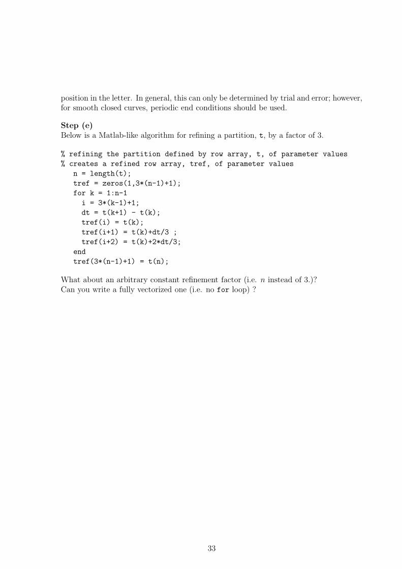
Step (e)Below is a Matlab-like algorithm for refining a partition, t, by a factor of 3.
% refining the partition defined by row array, t, of parameter values
% creates a refined row array, tref, of parameter values
n = length(t);
tref = zeros(1,3*(n-1)+1);
for k = 1:n-1
i = 3*(k-1)+1;
dt = t(k+1) - t(k);
tref(i) = t(k);
tref(i+1) = t(k)+dt/3 ;
tref(i+2) = t(k)+2*dt/3;
end
tref(3*(n-1)+1) = t(n);
What about an arbitrary constant refinement factor (i.e. n instead of 3.)?Can you write a fully vectorized one (i.e. no for loop) ?
33

34
4 Numerical Linear Algebra
4.1 From Equation Reduction to Triangular Factorization
“Gaussian elimination” for solving systems of linear equations has several meanings.Commonly, solving a linear systems of equations such as Ax = b is first learned via aprocess of reducing the given system of equations to a new system in which the unknowns,xi, are systematically eliminated. It may be necessary to re-order the equations toaccomplish this (equation pivoting).
However, the standard computer techniques referred to as “Gaussian elimination”for solving Ax = b are based on factoring A into triangular matrices, L and U . Thatis, these computer algorithms find non-singular N × N matrices L and U such thatA = LU . After the matrix factorization, the system can be solved in two steps: firstsolving Lz = b for z, followed by solving Ux = z for x. The factorization may not bepossible without re-ordering the equations. In matrix terms, re-ordering the equationsis accomplished by multiplying A and b by a ‘permutation’ matrix, P . Then, solvingthe equivalent system PAx = Pb can be done by factoring the matrix PA.
In this section, we show how these views are closely related. To do this, we discuss acommon intermediate view that is often used in elementary teaching about solving linearsystems of equations, the augmented matrix notation. The role here of the discussionof the augmented matrix procedure is that it enables us to move from manipulatingequations as per the equation reduction view to a matrix operations description. Thisin turn leads to the concepts of matrix factorization.
4.1.1 Reducing a system of equations
The elementary equation reduction form of Gaussian elimination can be summarized asfollows. Let E1, E2, . . . , EN represent the N equations in the system of equations.
Step one:The first step of the reduction process aims to eliminate x1 from all the N equationsexcept for E1.
For n→2 to Nreplace En by En − An,1
A1,1E1
End for
The result is a new system with
1) a subsystem of N − 1 new equations in unknowns (x2, x3, . . . , xN ), and
2) a single equation involving (x1, x2, . . . , xN ).
The solution of the new and old systems are the same.
The next step of the reduction, which is the final step, uses the first step recursively!
35
a) Apply “step one” to the smaller subsystem of N − 1 equations in (1) involvingthe variables (x2, x3, . . . , xN). However, instead of eliminating x1 (which is alreadygone), eliminate x2.Do this step recursively until you arrive at a system with only one equation andone unknown, xN . Thus, xN is known.
b) Use the known value of xN to solve the 2-equation system from the previousrecursion step. That is, solve for xN−1. Work your way back through the recursionsteps, and eventually solve for x1 using (x2, x3, . . . , xN).
After k invocations of the recursion of the reduction process, we have
• a subsystem of N − k equations in unknowns (xk+1, . . . , xN), and
• a subsystem of k equations. In this subsystem, the first equation involves allthe unknowns (x1, x2, . . . , xN). For each equation j (j = 2, . . . , k), the unknowns(x1, . . . , xj−1) have been eliminated.
Question: What if x1 does not appear in equation 1 (i.e A1,1 = 0)? Or if the same thinghappens in trying to apply subsequent reductions?
4.1.2 Augmented Matrix Notation and Row Reduction
Matrix notation was originally introduced to avoid explicitly writing down the symbolsfor the unknowns (x1, . . . , xk). This made pencil and paper calculations faster. Butmatrix notation is also useful for expressing the equation reduction process in terms ofmatrix multiplications.
Here we define the augmented system matrix as the N × (N + 1) matrix
A = [A, b] .
Step one of the equation reduction process can be described in terms of the followingrow reduction operations.
For n→2 to Nreplace row n by
(
row n− An,1
A1,1row 1
)
End for
This row reduction step can be expressed mathematically as a matrix multiplication bythe N ×N matrix M (1),
[A(1), b(1)] = M (1)A .
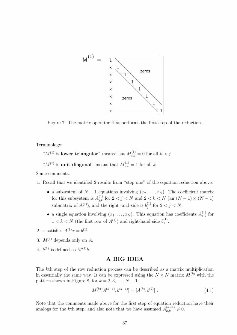
The pattern of entries in M (1) is as shown in Figure 7, where each ‘x’ in the first columnrepresents a non-zero number.
To pick a specific case, do you see why M(1)3,1 =
−A3,1
A1,1? And so in general M
(1)k,1 =
−Ak,1
A1,1
for k = 2, . . . , N .
36
1
x
x
1
1
1
1
1
1
1
x
x
x
x
xzeros
zeros
(1)=M
Figure 7: The matrix operator that performs the first step of the reduction.
Terminology:
“M (1) is lower triangular” means that M(1)j,k = 0 for all k > j
“M (1) is unit diagonal” means that M(1)k,k = 1 for all k
Some comments:
1. Recall that we identified 2 results from “step one” of the equation reduction above:
• a subsystem of N − 1 equations involving (x2, . . . , xN ). The coefficient matrix
for this subsystem is A(1)j,k for 2 < j < N and 2 < k < N (an (N − 1)× (N − 1)
submatrix of A(1)), and the right -and side is b(1)j for 2 < j < N ;
• a single equation involving (x1, . . . , xN). This equation has coefficients A(1)1,k for
1 < k < N (the first row of A(1)) and right-hand side b(1)1 .
2. x satisfies A(1)x = b(1).
3. M (1) depends only on A.
4. b(1) is defined as M (1)b.
A BIG IDEA
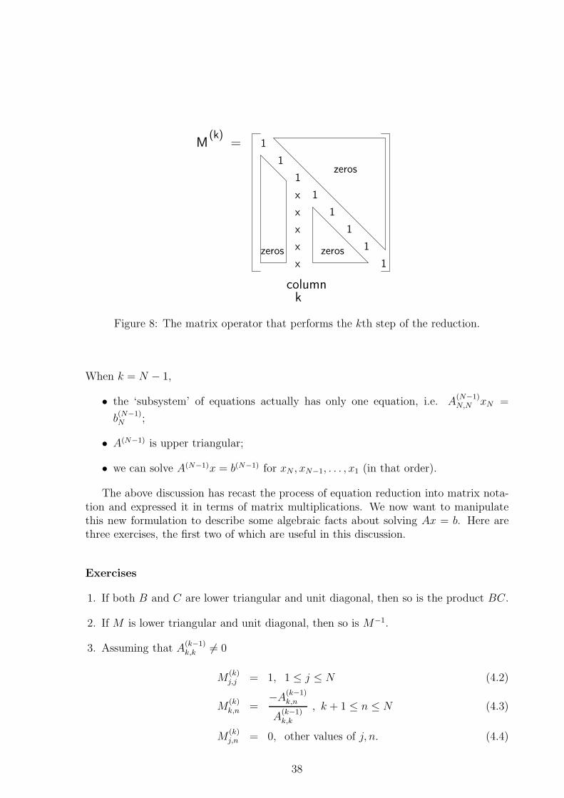
The kth step of the row reduction process can be described as a matrix multiplicationin essentially the same way. It can be expressed using the N ×N matrix M (k) with thepattern shown in Figure 8, for k = 2, 3, . . . , N − 1.
M (k)[A(k−1), b(k−1)] = [A(k), b(k)] . (4.1)
Note that the comments made above for the first step of equation reduction have theiranalogs for the kth step, and also note that we have assumed A
(k−1)k,k 6= 0.
37
1
1
1
1
1
1
1
1
zeros
=M
x
x
x
x
x
(k)
columnk
zeroszeros
Figure 8: The matrix operator that performs the kth step of the reduction.
When k = N − 1,
• the ‘subsystem’ of equations actually has only one equation, i.e. A(N−1)N,N xN =
b(N−1)N ;
• A(N−1) is upper triangular;
• we can solve A(N−1)x = b(N−1) for xN , xN−1, . . . , x1 (in that order).
The above discussion has recast the process of equation reduction into matrix nota-tion and expressed it in terms of matrix multiplications. We now want to manipulatethis new formulation to describe some algebraic facts about solving Ax = b. Here arethree exercises, the first two of which are useful in this discussion.
Exercises
1. If both B and C are lower triangular and unit diagonal, then so is the product BC.
2. If M is lower triangular and unit diagonal, then so is M−1.
3. Assuming that A(k−1)k,k 6= 0
M(k)j,j = 1, 1 ≤ j ≤ N (4.2)
M(k)k,n =
−A(k−1)k,n
A(k−1)k,k
, k + 1 ≤ n ≤ N (4.3)
M(k)j,n = 0, other values of j, n. (4.4)
38
Define U = A(N−1); this is the standard designation of this upper triangular matrixin the context of Gaussian elimination.
The matrix description of the kth reduction step shown in (4.1) can be broken intotwo steps:
M (k)A(k−1) = A(k) and M (k)b(k−1) = b(k) . (4.5)
The first of these implies
A(k−1) = (M (k))−1A(k) , (4.6)
and the second implies
b(k−1) = (M (k))−1b(k) . (4.7)
If we look at (4.6) for k = N − 1, we see that A(N−2) =(
M (N−1))−1
A(N−1). In general,
A(N−k) =(
M (N−k+1))−1 (
M (N−k+2))−1 · · ·
(
M (N−1))−1
A(N−1). (4.8)
Each matrix inverse,(
M (N−j))−1
, j = 1, . . . , k − 1, in (4.8) is lower triangular and unitdiagonal (see Exercise 2 above). Moreover, the product of these matrices is also lowertriangular and unit diagonal (see Exercise 1 above). So, setting k = N − 1, and definingthe matrix J as the product of the inverse matrices in (4.8), and setting A(N−1) = U ,we have
A(1) = JU (4.9)
where J is a lower triangular and unit diagonal matrix, and U is an upper triangularmatrix. Finally, since
A =(
M (1))−1
A(1) =(
M (1))−1
J U , (4.10)
by defining L as the product(
M (1))−1
J , the matrix of coefficients of the original systemof equations can be written as a product of two factors,
A = LU , (4.11)
where L is a lower triangular, unit diagonal matrix, and U is an upper triangular matrix.
If we performed the same development on (4.7), we could conclude that
b = Lb(N−1) . (4.12)
Then, we can get the solution, x, by solving
Ux = b(N−1) . (4.13)
This triangular factorization is the matrix view of Gaussian elimination. By factoringthe system matrix A into upper and lower triangular factors, the solution can easily beextracted.
39
4.1.3 Matrix factorization form of Gaussian elimination
This view of Gaussian elimination has the following major steps:
1. Compute triangular factors L and U so that LU = A.
2. Solve Lz = b (see (4.12) and identify z with b(N−1)).
3. Solve Ux = z.
What we have shown in the preceding sections is that these steps are not only possible,but are, in fact, closely related to what is done by the elementary equation reductionprocess. The next section presents and analyzes algorithms for the computations ofthese three steps.
4.2 LU Factorization
Consider an N × N matrix A, a solution vector x and a right hand side vector b. Wewish to solve
Ax = b . (4.14)
The preceding section gave an overview of how the triangular factorization of A is relatedto the row reduction process, but not the details of how to carry out the computation.Here we present the algorithm for factoring A = LU , where L is unit lower triangular,and U is upper triangular.
Algorithm: LU FactorizationGiven an N ×N matrix A = aij
For k = 1, . . . , NFor i = k + 1, . . . , N
mult := aik/akk
aik := multFor j = k + 1, . . . , N
aij := aij −mult ∗ akj
EndForEndFor
EndFor
Note that in the above LU factorization algorithm, the original entries of A areoverwritten by L and U . The strictly lower part of the modified A array contains thestrictly lower part of L (the unit diagonal is understood). The upper triangular part ofthe A array now contains U . This convention is common among implementations of theLU factorization algorithm because it requires no extra storage.
To solve equation (4.14), we note that
Ax = LUx = b . (4.15)
40
If we define z = Ux, then it follows from equation (4.15) that
Lz = b , (4.16)
Ux = z . (4.17)
Equations (4.16) and (4.17) are easy to solve. Let the entries of (L)ij = lij , where werecall that L is unit lower triangular. We can easily solve Lz = b for z using the forwardsolve algorithm:
Algorithm: Forward SolveFor i = 1, . . . , N
zi := bi
For j = 1, . . . , i− 1zi := zi − lij ∗ zj
EndForEndFor
Let the entries of (U)ij = uij. We can easily solve Ux = z for x using the back solvealgorithm:
Algorithm: Back SolveFor i = N, . . . , 1
xi := zi
For j = i + 1, . . . , Nxi := xi − uij ∗ xj
EndForxi := xi/uii
EndFor
One of the advantages of factoring A = LU is that we can solve for multiple right-hand sides simply by doing multiple forward and back solves. Can you think of anefficient way to form A−1 given that you have already found A = LU?
4.2.1 How do we count work?
The running time of the above algorithms will be proportional to the number of flops.Notice that most statements consist of linked triad operations such as
zi := zi − lij ∗ zj .
That is, usually multiplication is paired with an addition or subtraction. So, oftena measure of work is to simply count the number of multiply-adds. Usually, the totalnumber of multiply-adds is about one-half the total number of additions+subtractions+multiplies + divides. In fact, both operation counts are called number of flops. Thereis no standard agreement on this terminology. We shall adopt the Matlab convention,
41
which is to count the total number of operations, i.e. one multiply-add is two flops. Theflop count will include the total number of adds + multiplies + divides + subtracts. Asimple calculation gives the total number of flops for factoring an N ×N matrix:
LU Factorization Work =2N3
3+ O(N2) flops
= O(N3) flops. (4.18)
The flop count for the Forward Solve plus Back Solve is:
Forward + Back Solve Work = 2N2 + O(N)
= O(N2). (4.19)
Obviously, for large N , the factorization process is more expensive than the forward/backsolve.
4.2.2 Pivoting and the Stability of Factorization
Each of the closely related views of Gaussian elimination given in the opening section canfail if a division by zero is encountered at some stage. This problem can be sidesteppedif we carry out some form of row pivoting.
For the equation reduction view, row pivoting defines a re-ordering of the equations.For the augmented matrix view, it has the effect of re-ordering the rows of [A(k), b(k)].This operation can be described in matrix terms as a multiplication by a permutationmatrix. A permutation matrix is a matrix of 0s and 1s. Each row of a permutationmatrix contains exactly one 1 (all the other elements are 0s). The same is true for eachcolumn of a permutation matrix. For example, the permutation matrix that interchangesthe second and third rows of a 3× 3 matrix is
P =
1 0 00 0 10 1 0
.
Try multiplying a 3× 3 matrix by P to see how it works.In the LU factorization algorithm, if a
(k)kk = 0 at some stage, then we examine all
entries in the kth column below a(k)kk to find the element with the largest absolute value.
Suppose |a(k)τk | is the largest, i.e.
maxj=k,..,N
|a(k)jk | = |a
(k)τk | . (4.20)
Then we swap row τ with row k, and use a(k)τk to form the multiplier. This process is
called pivoting. Note that at least one of a(k)kk , a
(k)k+1,k, . . . , a
(k)Nk must be nonzero, otherwise
the matrix is singular. Row-swapping produces a re-ordering of the rows of A that couldbe described by a permutation matrix, P . This same re-ordering is applied to the right-hand side vector b. As a result, we get the new system of equations, PAx = Pb, havingthe same solution, x, as the original system, Ax = b.
42
Algorithmically, the process of pivoting is intertwined with the factorization to pro-duce P , L, and U from A.
Standard computer oriented algorithms for solving Ax = b have two stages:
(a) from A, compute P , L and U such that PA = LU ;
(b) from P , L, U and b, compute x.
The amount of work required for stage (a) is 2N3
3 +O(N2) flops, while stage (b) requires
2N2 + O(N) flops.
In Matlab, stage (a) can be done using the lu(A) command:
[L,U,P] = lu(A) .
4.2.3 Stability
So far, we have been discussing the factorization algorithm as it operates using math-ematically exact arithmetic. What happens when we implement the algorithm in theinexact arithmetic of a floating point number system? Could errors build up during theO(N3) arithmetic operations of the factorization?
The following is a general rule of thumb concerning the behaviour of algorithmsimplemented in inexact (floating point) arithmetic.
If an algorithm fails under some condition when exact arithmetic is used,then, if the algorithm is implemented using inexact arithmetic, it can generatelarge errors when the failure condition is approximately true.
The algorithm of interest here is the LU factorization of matrix A. Using exact arith-metic, it can fail if a
(k)kk = 0 at some stage. The rule of thumb says that a program to
implement it in floating point arithmetic can generate large errors if |a(k)kk | is very small.
(So what constitutes being small? )
However, if we add row pivoting to the LU factorization algorithm, then, in exactarithmetic, the resulting algorithm only fails if the row pivoting fails to find a non-zeroentry anywhere on or below the diagonal in column k of A(k). So we can expect thefactorization computed in floating point to be reasonably accurate unless all the entriesof A(k) on or below the diagonal in column k are small, not just A
(k)kk itself.
A measure of the stability of factorization is
ρ = maxi,j,k|a(k)
ij |, (4.21)
i.e. if the size of the maximum entry in A(k) becomes very large during the course ofelimination, then this indicates that small pivots are encountered.
43
4.3 Matrix and Vector Norms
Before we continue, we give a short overview of matrix and vector norms. The norm ofa vector is a measure of its size. Let x be the vector
x =
x1
x2...
xn
. (4.22)
Then we define the 1-norm, 2-norm, and ∞-norm as
‖x‖1 =
n∑
i=1
|xi|
‖x‖2 =
(
n∑
i=1
x2i
)1/2
‖x‖∞ = maxi|xi| .
Usually, these types of norms are referred to as p-norms
‖x‖p where p = 1, 2,∞ . (4.23)
Matlab computes these vector norms using the norm command.
Properties of Norms
‖x‖ = 0 iff xi = 0 ∀i‖αx‖ = |α| ‖x‖ , α = scalar
‖x + y‖ ≤ ‖x‖+ ‖y‖
Matrix NormsWe define a matrix norm for an n× n matrix A corresponding to a given vector norm,as follows:
‖A‖p = max‖x‖6=0
‖Ax‖p‖x‖p
for any ‖ · ‖p norm. It can be shown that (see any linear algebra text)
‖A‖1 = maxj
n∑
i=1
|aij|
= max absolute column sum
‖A‖∞ = maxi
n∑
j=1
|aij|
= max absolute row sum.
44
For the ‖ · ‖2 norm, we have to consider the eigenvalues of A. Recall that A has aneigenvalue λ (a scalar) associated with a nonzero vector x if
Ax = λx,
where the vector x is the eigenvector associated with the eigenvalue λ. If λi, i = 1, .., nare the eigenvalues of AtA, then
‖A‖2 = maxi|λi|1/2.
Matlab also computes these matrix norms via the norm command.Note that for any n× n matrices A and B, and any n-vector x, we have
‖A‖ = 0 iff aij = 0 ∀i, j‖αA‖ = |α| ‖A‖ , α = scalar
‖A + B‖ ≤ ‖A‖+ ‖B‖‖Ax‖ ≤ ‖A‖ ‖x‖‖AB‖ ≤ ‖A‖ ‖B‖‖I‖ = 1 , I = identity matrix.
4.4 Condition Numbers
4.4.1 Conditioning
Suppose we perturb the right-hand-side vector b in
Ax = b.
What happens to x? Let’s replace b by b+∆b, which means that x will change to x+∆x,which gives
A(x + ∆x) = b + ∆b. (4.24)
Since if x is the exact solution, then Ax = b, so that equation (4.24) becomes
∆x = A−1∆b. (4.25)
Noting that Ax = b, so that
‖b‖ ≤ ‖A‖‖x‖, (4.26)
and from equation (4.25) we obtain
‖∆x‖ ≤ ‖A−1‖‖∆b‖. (4.27)
Now, equation (4.26) gives
‖x‖ ≥ ‖b‖‖A‖ or‖A‖‖b‖ ≥
1
‖x‖ . (4.28)
45
Equations (4.27) and (4.28) give
‖∆x‖‖x‖ ≤ ‖A‖ ‖A−1‖‖∆b‖
‖b‖ . (4.29)
Note that the above is true for any ‖ · ‖p norm.Let κ(A) = ‖A‖‖A−1‖ be the condition number of A. So, equation (4.29) says
that
relative change in x ≤ condition number × relative change in b.
If κ(A) is large, then the problem may be ill-conditioned; since the bound is not verysharp, κ(A) may grossly overestimate the problem. On the other hand, if κ(A) is small(near one), then, for sure the problem is well-conditioned.
Now, suppose we perturb the matrix elements A, i.e.
(A + ∆A)(x + ∆x) = b, (4.30)
then, assuming Ax = b, i.e. x is the exact solution, equation (4.30) implies
A∆x = −∆A(x + ∆x)
∆x = −A−1 [∆A(x + ∆x)] , (4.31)
which then gives
‖∆x‖ ≤ ‖A−1‖‖∆A‖‖x + ∆x‖, (4.32)
or
‖∆x‖‖x + ∆x‖ ≤ ‖A−1‖‖A‖‖∆A‖
‖A‖
= κ(A)‖∆A‖‖A‖ . (4.33)
Once again the condition number appears. So, a measure of the sensitivity to changesin A or b is the condition number. Note that
• κ(A) ≥ 1;
• κ(αA) = κ(A), α = scalar.
4.4.2 The residual
The accuracy of the computed solution is sometimes measured by the size of the residualwhich is defined as follows. If the computed solution for the system Ax = b is x + ∆x(it is not exact) then the residual is
r = b− A(x + ∆x) . (4.34)
46
If the residual r = 0 then ∆x = 0 and we have the exact solution. From equation (4.34)we have
A(x + ∆x) = b− r .
Similar analysis as in equations (4.24-4.29) gives
‖∆x‖‖x‖ ≤ κ(A)
‖r‖‖b‖ . (4.35)
Thus a small residual does not necessarily imply a small error, if κ(A) is large. Forexample, it is unavoidable that
‖r‖‖b‖ ≃ εmachine (4.36)
in which case equation (4.35) implies
‖∆x‖‖x‖ ≤ κ(A) εmachine
which may not be small if the problem is poorly conditioned.For implementation in floating point arithmetic, Gaussian elimination with pivoting
is known to be a stable method. Moreover, it yields a computed result whose residualis small, namely, the residual is approximately the size indicated by equation (4.36) inmost cases. For this reason, it is a commonly used method.
Another type of analysis known as “backward error analysis” yields the following re-sult. Gaussian elimination with pivoting produces a computed solution x which satisfies
(A + E)x = b
where ‖E‖ = εmachine ‖A‖. In other words, Gaussian elimination with pivoting solves anearby problem exactly. From equation (4.33) we have
‖x− x‖‖x‖ ≤ κ(A) εmachine .
As stated before, the condition number is a property of the problem and not a propertyof the algorithm used to solve the problem. We conclude that the result computedin a floating point number system via Gaussian elimination with pivoting is about asaccurate as could ever be achieved. However, the computed solution may not be closeto the true solution if the problem has a large condition number.
47

48
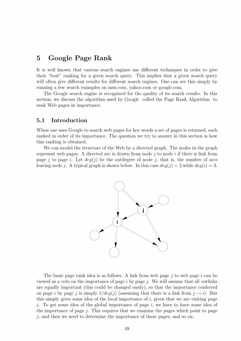
5 Google Page Rank
It is well known that various search engines use different techniques in order to givetheir “best” ranking for a given search query. This implies that a given search querywill often give different results for different search engines. One can see this simply byrunning a few search examples on msn.com, yahoo.com or google.com.
The Google search engine is recognized for the quality of its search results. In thissection, we discuss the algorithm used by Google called the Page Rank Algorithm torank Web pages in importance.
5.1 Introduction
When one uses Google to search web pages for key words a set of pages is returned, eachranked in order of its importance. The question we try to answer in this section is howthis ranking is obtained.
We can model the structure of the Web by a directed graph. The nodes in the graphrepresent web pages. A directed arc is drawn from node j to node i if there is link frompage j to page i. Let deg(j) be the outdegree of node j, that is, the number of arcsleaving node j. A typical graph is shown below. In this case deg(j) = 2 while deg(i) = 3.
i
j
The basic page rank idea is as follows. A link from web page j to web page i can beviewed as a vote on the importance of page i by page j. We will assume that all outlinksare equally important (this could be changed easily), so that the importance conferredon page i by page j is simply 1/deg(j) (assuming that there is a link from j → i). Butthis simply gives some idea of the local importance of i, given that we are visiting pagej. To get some idea of the global importance of page i, we have to have some idea ofthe importance of page j. This requires that we examine the pages which point to pagej, and then we need to determine the importance of these pages, and so on.
49
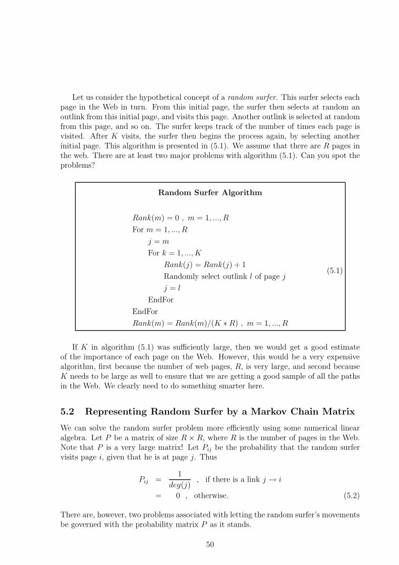
Let us consider the hypothetical concept of a random surfer. This surfer selects eachpage in the Web in turn. From this initial page, the surfer then selects at random anoutlink from this initial page, and visits this page. Another outlink is selected at randomfrom this page, and so on. The surfer keeps track of the number of times each page isvisited. After K visits, the surfer then begins the process again, by selecting anotherinitial page. This algorithm is presented in (5.1). We assume that there are R pages inthe web. There are at least two major problems with algorithm (5.1). Can you spot theproblems?
Random Surfer Algorithm
Rank(m) = 0 , m = 1, ..., R
For m = 1, ..., R
j = m
For k = 1, ..., K
Rank(j) = Rank(j) + 1
Randomly select outlink l of page j
j = l
EndFor
EndFor
Rank(m) = Rank(m)/(K ∗R) , m = 1, ..., R
(5.1)
If K in algorithm (5.1) was sufficiently large, then we would get a good estimateof the importance of each page on the Web. However, this would be a very expensivealgorithm, first because the number of web pages, R, is very large, and second becauseK needs to be large as well to ensure that we are getting a good sample of all the pathsin the Web. We clearly need to do something smarter here.
5.2 Representing Random Surfer by a Markov Chain Matrix
We can solve the random surfer problem more efficiently using some numerical linearalgebra. Let P be a matrix of size R× R, where R is the number of pages in the Web.Note that P is a very large matrix! Let Pij be the probability that the random surfervisits page i, given that he is at page j. Thus
Pij =1
deg(j), if there is a link j → i
= 0 , otherwise. (5.2)
There are, however, two problems associated with letting the random surfer’s movementsbe governed with the probability matrix P as it stands.
50
5.2.1 Dead End Pages
What happens if page i has no outlinks? In this case, once our random surfer visits pagei, he will have no way of leaving this page. To avoid this problem, we suppose that therandom surfer teleports to another page at random, if he encounters a dead end page.We suppose that this teleportation moves the surfer to any other page in the Web withequal probability. More precisely, let d be an R dimensional column vector such that
[d]i = 1 , if deg(i) = 0
= 0 , otherwise (5.3)
and let e = [1, 1, ..., 1]t be the R dimensional column vector of ones. Then we define anew matrix P ′ of transition probabilities to include the teleportation property, as follows:
P ′ = P +1
Re · dt . (5.4)
5.2.2 Cycling Pages
Suppose that page j contains only a link to page i, and page i contains only a link topage j. This will trap our random surfer in an endless cycle. We will again use theteleportation idea to make sure that the random surfer can escape from the boredomof visiting the same pages in cyclic fashion. Let 0 < α < 1 (Google uses α = .85), anddefine a new matrix of probabilities
M = αP ′ + (1− α) · 1
Re · et . (5.5)
What does equation (5.5) do? Essentially, we are saying that the surfer moves to otherpages based on the usual idea of selecting an outlink at random, and, in addition, thesurfer can also teleport any other page on the web with equal probability. We weightthe usual outlink probabilities by α, and the teleportation probability by (1−α), so thatthe total probability of visiting the next page on the web is one. Once again, we caninterpret Mij as the probability that the random surfer will move from page j to page i.Note that from the definition of M we have that 0 < Mij ≤ 1, and
∑
i
Mij = 1 ; (5.6)
i.e., each column sums to 1 (colsum(M) = 1). In other words, given that the randomsurfer is at page j, then the probability that he will end up at some new page is one.
The matrix M defined by equation (5.5) is referred to as the Google Matrix.
51
5.3 Markov Transition Matrices
Let us be a bit more formal here.
Definition 5.1 A matrix Q is a Markov matrix if
0 ≤ Qij ≤ 1 and∑
i
Qij = 1 . (5.7)
Obviously, matrix M in equation (5.5) is a Markov matrix. Let [p]i represent theprobability that the random surfer is at page i so that p is an R dimensional columnvector. We could, for example, specify that initially
[p]i =1
R, ∀i (5.8)
that is, the random surfer visits each page initially with equal probability.
Definition 5.2 A vector q is a probability vector if
0 ≤ [q]i ≤ 1 and∑
i
[q]i = 1 . (5.9)
Given that, at hop n, the random surfer is in the state represented by the probabilityvector pn, that is, the probability that the surfer is at page i is [pn]i, then the probabilityvector at state n + 1 is
pn+1 = Mpn . (5.10)
We should verify that pn+1 is a probability vector. Since M is a Markov matrix, and pn
is a probability vector, then we have that
[pn+1]i ≥ 0 , ∀i (5.11)
and as well
∑
i
[pn+1]i =∑
i
∑
j
Mij [pn]j
=∑
j
[pn]j∑
i
Mij
=∑
j
[pn]j
= 1 . (5.12)
Thus pn a probability vector implies then pn+1 is also a probability vector for each n.
52
5.4 Page Rank
Given the assumption above, we can now precisely state the algorithm for determiningthe ranking of each page in the Web. Let
p0 =1
Re (5.13)
(that is, the random surfer visits each page initially with equal probability). Then therank of page i is given by [p]∞i where
p∞ = limk→∞
(M)kp0 . (5.14)
So, essentially, we start with p0 defined by equation (5.13) and then repeatedlymultiply by M , to give us p∞. There are two obvious questions
• Does iteration (5.14) converge?
• If yes, how fast does this iteration converge?
5.5 Convergence Analysis
In order to analyze the convergence of iteration (5.14), we have to review some basiclinear algebra. (Maybe you haven’t seen this before, but its easy). Suppose we have aspecial vector x such that
Qx = λx (5.15)
where λ is a (possibly complex) nonzero scalar. The special vector x is an eigenvectorof the matrix Q, with eigenvalue λ.
Note that equation (5.15) is equivalent to finding a nonzero solution of the linearsystem of equations (λI − Q)x = 0 and so λ an eigenvalue of Q is equivalent to thematrix λI − Q being singular. This in turn implies that eigenvalues are roots of thecharacteristic polynomial det(λI −Q) of Q.
5.5.1 Some Technical Results
We are going to very briefly derive some technical properties of the eigenvalues of aMarkov matrix here. If you are not a linear algebra fan, I suggest you skip to Section5.5.2.
Theorem 5.3 Every Markov matrix Q has 1 as an eigenvalue.
Proof: The eigenvalues of Q and Qt are the same (since Q and Qt have the samecharacteristic polynomials). Since Qte = e, we have that λ = 1 is an eigenvalue of Qt.Thus λ = 1 is an eigenvalue of Q.
Theorem 5.4 Every (possibly complex) eigenvalue λ of a Markov matrix Q satisfies
|λ| ≤ 1 . (5.16)
Thus 1 is the largest eigenvalue of Q.
53
Proof: This result actually follows from the Gershgorin Circle Theorem (a resultthat can be found in optimization texts) applied to the eigenvalues of Qt. Since theeigenvalues of Q and Qt are the same, the theorem follows.
Definition 5.5 A Markov matrix Q is a positive Markov matrix if
Qij > 0 , ∀i, j . (5.17)
Theorem 5.6 If Q is a positive Markov matrix, then there is only one eigenvector ofQ with |λ| = 1.
Proof: See, for example, (Grimmett and Stirzaker, Probability and Random Pro-cesses, Oxford University Press, 1989.)
5.5.2 Convergence Proof
Theorem 5.7 If M is a positive Markov matrix, the iteration (5.14) converges to aunique vector p∞, for any initial probability vector p0.
Proof: Let xl be an eigenvector of M , corresponding to the eigenvalue λl. Supposethat M has a complete set of eigenvectors, in other words, we can represent p0 as
p0 =∑
l
clxl (5.18)
for some scalars cl. (We do not have to make this assumption, but it simplifies theproof). Suppose also that we order these eigenvectors so that |λ1| > |λ2| ≥ ... so thatx1 corresponds to the unique eigenvector with λ1 = 1. Then
(M)kp0 = c1x1 +
R∑
l=2
cl(λl)kxl . (5.19)
From Theorem (5.6), we have that |λl| < 1 for all l > 1, so that
limk→∞
(M)kp0 = c1x1 (5.20)
for any p0. c1x1 cannot be identically zero, since p0 is a probability vector, and hencep∞ is a probability vector. Hence c1 6= 0 and x1 cannot be the zero vector. Uniquenessfollows since if we start the iteration with another probability vector
q0 =∑
l
blxl (5.21)
for some coefficients bl, then
q∞ = limk→∞
(M)kq0 = b1x1 . (5.22)
But, for given x1, since q∞,p∞ are probability vectors, we have b1 = c1.
54
Remark 5.8 The speed of convergence of algorithm (5.14) is determined by the size ofthe second largest eigenvalue λ2 of the Google matrix M , since |λl| < |λ2|, l > 2. One canshow that the size of |λ2| ≃ α (see Golub and van Loan, Matrix Computations, 1996).For example, if α = .85, then |λ2|114 = (.85)114 ≃ 10−8. This means that 114 iterationsof algorithm (5.14) for any starting vector should give reasonably accurate estimates forp∞.
The Web is estimated to contain billions of pages. Using algorithm (5.14) is esti-mated to require several days of computation. Note that the ranking vector p∞ can becomputed and stored independent of the Google query. When a user enters a keywordsearch, a subset of Web pages containing the keywords is returned. Then, these pagesare ranked according to the precomputed vector p∞.
Why not just choose α very small, since this would speed up the computation?Consider the case α = 0. Then its easy to see that [p∞]i = 1/R, i.e. all pages areranked equally. The smaller the value of α, the faster the convergence of algorithm(5.14). However small values of α result in less significant ranking information.
5.6 Practicalities
If we assume that pn is a probability vector then
eet
Rpn =
1
Re(etpn)
=e
R(5.23)
so that
Mpn = αP ′pn + (1− α)e
R(5.24)
and that
P ′pn = (P +e · dt
R)pn
= Ppn + e(dtpn
R) . (5.25)
Putting these two steps together gives
Mpn = α(Ppn + e(dtpn
R)) + (1− α)
e
R. (5.26)
Typically, P is quite sparse, so that even though M is dense, we can perform the matrix-vector multiply Mpn in O(R) operations.
55
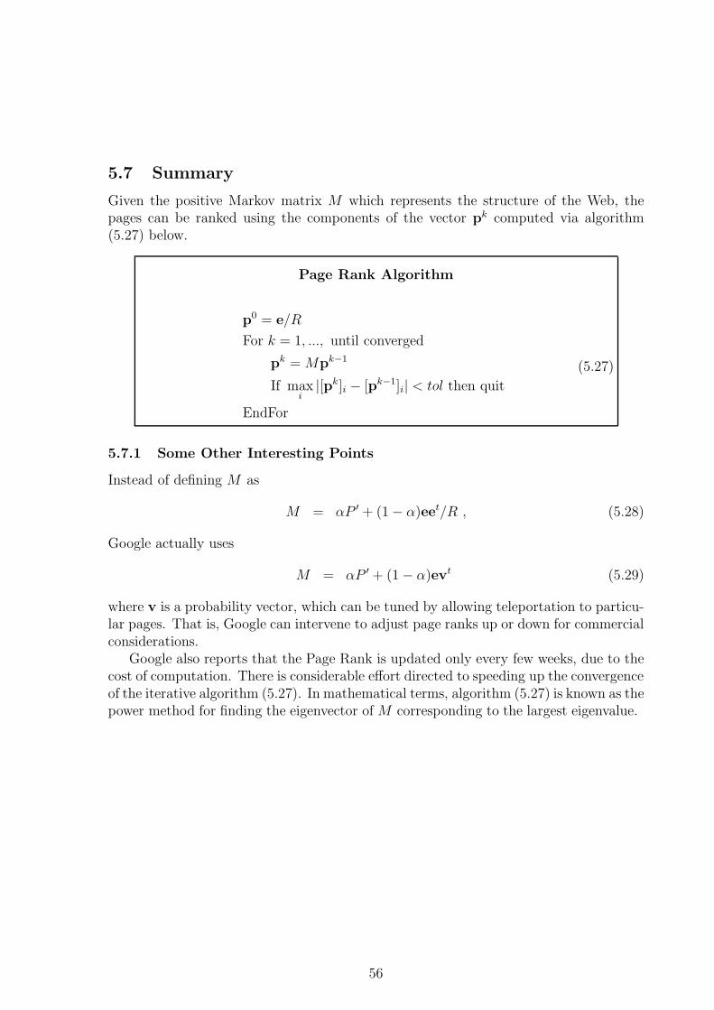
5.7 Summary
Given the positive Markov matrix M which represents the structure of the Web, thepages can be ranked using the components of the vector pk computed via algorithm(5.27) below.
Page Rank Algorithm
p0 = e/R
For k = 1, ..., until converged
pk = Mpk−1
If maxi|[pk]i − [pk−1]i| < tol then quit
EndFor
(5.27)
5.7.1 Some Other Interesting Points
Instead of defining M as
M = αP ′ + (1− α)eet/R , (5.28)
Google actually uses
M = αP ′ + (1− α)evt (5.29)
where v is a probability vector, which can be tuned by allowing teleportation to particu-lar pages. That is, Google can intervene to adjust page ranks up or down for commercialconsiderations.
Google also reports that the Page Rank is updated only every few weeks, due to thecost of computation. There is considerable effort directed to speeding up the convergenceof the iterative algorithm (5.27). In mathematical terms, algorithm (5.27) is known as thepower method for finding the eigenvector of M corresponding to the largest eigenvalue.
56
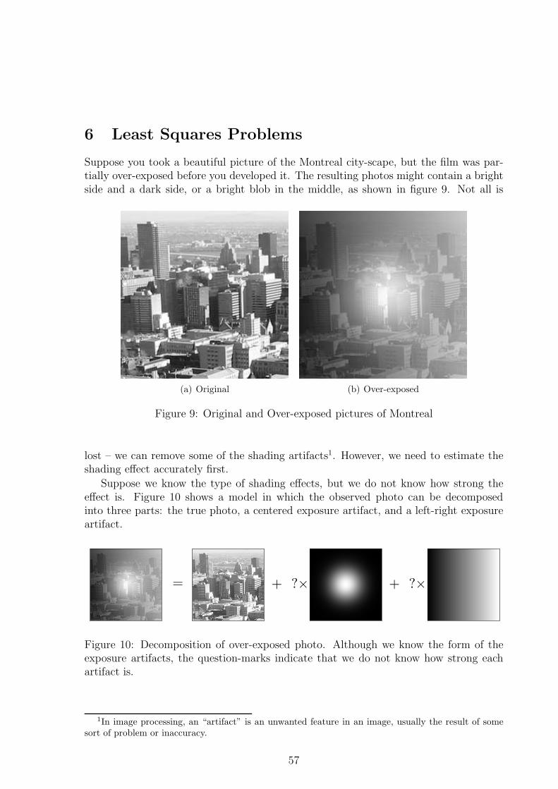
6 Least Squares Problems
Suppose you took a beautiful picture of the Montreal city-scape, but the film was par-tially over-exposed before you developed it. The resulting photos might contain a brightside and a dark side, or a bright blob in the middle, as shown in figure 9. Not all is
(a) Original (b) Over-exposed
Figure 9: Original and Over-exposed pictures of Montreal
lost – we can remove some of the shading artifacts1. However, we need to estimate theshading effect accurately first.
Suppose we know the type of shading effects, but we do not know how strong theeffect is. Figure 10 shows a model in which the observed photo can be decomposedinto three parts: the true photo, a centered exposure artifact, and a left-right exposureartifact.
+ ?× + ?×=
Figure 10: Decomposition of over-exposed photo. Although we know the form of theexposure artifacts, the question-marks indicate that we do not know how strong eachartifact is.
1In image processing, an “artifact” is an unwanted feature in an image, usually the result of somesort of problem or inaccuracy.
57
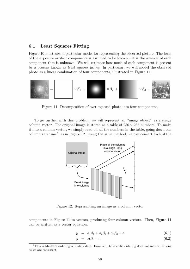
6.1 Least Squares Fitting
Figure 10 illustrates a particular model for representing the observed picture. The formof the exposure artifact components is assumed to be known – it is the amount of eachcomponent that is unknown. We will estimate how much of each component is presentby a process known as least squares fitting. In particular, we will model the observedphoto as a linear combination of four components, illustrated in Figure 11.
= ×β3 +×β2 +×β1 +
Figure 11: Decomposition of over-exposed photo into four components.
To go further with this problem, we will represent an “image object” as a singlecolumn vector. The original image is stored as a table of 256× 256 numbers. To makeit into a column vector, we simply read off all the numbers in the table, going down onecolumn at a time2, as in Figure 12. Using the same method, we can convert each of the
Original image
Break image
into columns
Place all the columns
in a single, long
column vector.
...
Figure 12: Representing an image as a column vector
components in Figure 11 to vectors, producing four column vectors. Then, Figure 11can be written as a vector equation,
y = a1β1 + a2β2 + a3β3 + ǫ (6.1)
y = Aβ + ǫ , (6.2)
2This is Matlab’s ordering of matrix data. However, the specific ordering does not matter, as longas we are consistent.
58
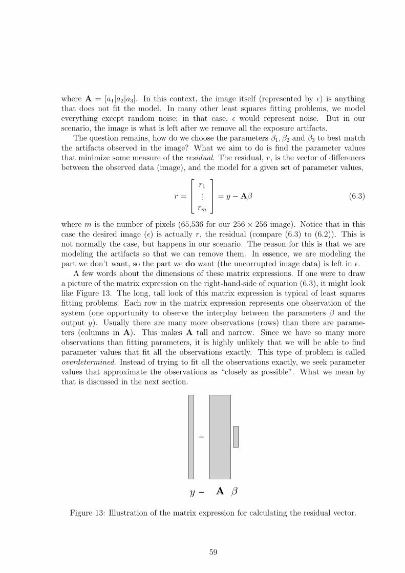
where A = [a1|a2|a3]. In this context, the image itself (represented by ǫ) is anythingthat does not fit the model. In many other least squares fitting problems, we modeleverything except random noise; in that case, ǫ would represent noise. But in ourscenario, the image is what is left after we remove all the exposure artifacts.
The question remains, how do we choose the parameters β1, β2 and β3 to best matchthe artifacts observed in the image? What we aim to do is find the parameter valuesthat minimize some measure of the residual. The residual, r, is the vector of differencesbetween the observed data (image), and the model for a given set of parameter values,
r =
r1...
rm
= y −Aβ (6.3)
where m is the number of pixels (65,536 for our 256× 256 image). Notice that in thiscase the desired image (ǫ) is actually r, the residual (compare (6.3) to (6.2)). This isnot normally the case, but happens in our scenario. The reason for this is that we aremodeling the artifacts so that we can remove them. In essence, we are modeling thepart we don’t want, so the part we do want (the uncorrupted image data) is left in ǫ.
A few words about the dimensions of these matrix expressions. If one were to drawa picture of the matrix expression on the right-hand-side of equation (6.3), it might looklike Figure 13. The long, tall look of this matrix expression is typical of least squaresfitting problems. Each row in the matrix expression represents one observation of thesystem (one opportunity to observe the interplay between the parameters β and theoutput y). Usually there are many more observations (rows) than there are parame-ters (columns in A). This makes A tall and narrow. Since we have so many moreobservations than fitting parameters, it is highly unlikely that we will be able to findparameter values that fit all the observations exactly. This type of problem is calledoverdetermined. Instead of trying to fit all the observations exactly, we seek parametervalues that approximate the observations as “closely as possible”. What we mean bythat is discussed in the next section.
y A β
Figure 13: Illustration of the matrix expression for calculating the residual vector.
59
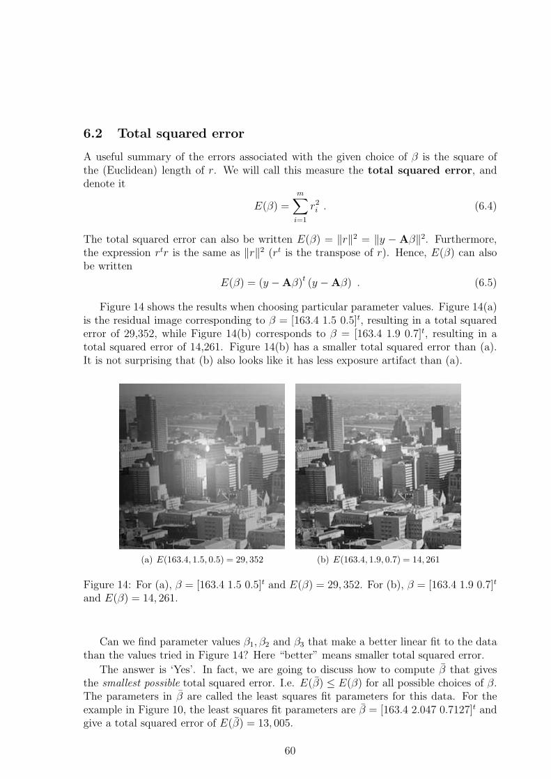
6.2 Total squared error
A useful summary of the errors associated with the given choice of β is the square ofthe (Euclidean) length of r. We will call this measure the total squared error, anddenote it
E(β) =
m∑
i=1
r2i . (6.4)
The total squared error can also be written E(β) = ‖r‖2 = ‖y − Aβ‖2. Furthermore,the expression rtr is the same as ‖r‖2 (rt is the transpose of r). Hence, E(β) can alsobe written
E(β) = (y −Aβ)t (y −Aβ) . (6.5)
Figure 14 shows the results when choosing particular parameter values. Figure 14(a)is the residual image corresponding to β = [163.4 1.5 0.5]t, resulting in a total squarederror of 29,352, while Figure 14(b) corresponds to β = [163.4 1.9 0.7]t, resulting in atotal squared error of 14,261. Figure 14(b) has a smaller total squared error than (a).It is not surprising that (b) also looks like it has less exposure artifact than (a).
(a) E(163.4, 1.5, 0.5) = 29, 352 (b) E(163.4, 1.9, 0.7) = 14, 261
Figure 14: For (a), β = [163.4 1.5 0.5]t and E(β) = 29, 352. For (b), β = [163.4 1.9 0.7]t
and E(β) = 14, 261.
Can we find parameter values β1, β2 and β3 that make a better linear fit to the datathan the values tried in Figure 14? Here “better” means smaller total squared error.
The answer is ‘Yes’. In fact, we are going to discuss how to compute β that givesthe smallest possible total squared error. I.e. E(β) ≤ E(β) for all possible choices of β.The parameters in β are called the least squares fit parameters for this data. For theexample in Figure 10, the least squares fit parameters are β = [163.4 2.047 0.7127]t andgive a total squared error of E(β) = 13, 005.
60
6.3 The Normal Equations
There is a simple method to finding the optimal least squares fit parameters for a linearleast squares problem. If the model is a linear function of the parameters (i.e. if themodel can be written as a matrix times the vector of parameters values), then thismethod is guaranteed to find the least squares solution.
To find the least squares solution, we need to solve the normal equations. Thissection describes what the normal equations are, and where they come from. You willsee that it is nothing more than first-year calculus.
In calculus, if you want to find the minimum value of a function f(x), you take thederivative and set it equal to zero. The same methodology applies to higher-dimensionalfunctions, such as our total squared error function, E(β). The definition of the (direc-tional) derivative of E(β) is
∂E
∂β= lim
e→0
E(β + e)−E(β)
‖e‖ . (6.6)
The numerator of (6.6) can be written
E(β + e)− E(β)
= (y −A(β + e))t (y −A(β + e))− (y −Aβ)t (y −Aβ)
=(
yt − (β + e)tAt)
(y −A(β + e))−(
yt − βtAt)
(y −Aβ)
= yty − ytA(β + e)− (β + e)tAty + (β + e)tAtA(β + e)
−yty + ytAβ + βtAty − βtAtAβ
= −ytA(β + e)− (β + e)tAty + (β + e)tAtA(β + e) + ytAβ + βtAty − βtAtAβ
= −ytAβ − ytAe− βtAty − etAty + (β + e)tAtA(β + e) + ytAβ + βtAty − βtAtAβ
= −ytAe− etAty + (β + e)tAtA(β + e)− βtAtAβ
= −2etAty + (β + e)tAtA(β + e)− βtAtAβ (since ytAe = etAty)
= −2etAty + βtAtAβ + βtAtAe + etAtAβ + etAtAe− βtAtAβ
= −2etAty + 2βtAtAe + etAtAe (since βtAtAe + etAtAβ)
= 2et(
AtAβ −Aty)
+ etAtAe .
Phew! Now we can write (6.6) as
∂E
∂β= lim
e→0
2et (AtAβ −Aty) + etAtAe
‖e‖ (6.7)
= lime→0
2et (AtAβ −Aty)
‖e‖ + lime→0
etAtAe
‖e‖ (6.8)
= 0 (6.9)
The second limit in (6.8) is zero, since
0 ≤ lime→0
etAtAe
‖e‖ ≤ lime→0
‖e‖2‖A‖2‖e‖ = ‖A‖2 lim
e→0‖e‖ = 0 . (6.10)
61
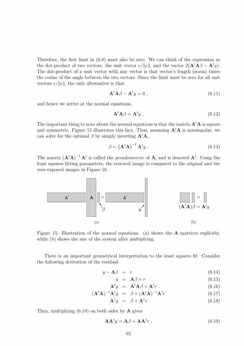
Therefore, the first limit in (6.8) must also be zero. We can think of the expression asthe dot-product of two vectors: the unit vector e/‖e‖, and the vector 2(AtAβ −Aty).The dot-product of a unit vector with any vector is that vector’s length (norm) timesthe cosine of the angle between the two vectors. Since the limit must be zero for all unitvectors e/‖e‖, the only alternative is that
AtAβ −Aty = 0 , (6.11)
and hence we arrive at the normal equations,
AtAβ = Aty . (6.12)
The important thing to note about the normal equations is that the matrix AtA is squareand symmetric. Figure 15 illustrates this fact. Thus, assuming AtA is nonsingular, wecan solve for the optimal β by simply inverting AtA,
β =(
AtA)−1
Aty . (6.13)
The matrix (AtA)−1
At is called the pesudoinverse of A, and is denoted A†. Using theleast squares fitting parameters, the restored image is compared to the original and theover-exposed images in Figure 16.
β
AA′
A′
y
(a)
(A′A)β = A
′y
(b)
Figure 15: Illustration of the normal equations. (a) shows the A matrices explicitly,while (b) shows the size of the system after multiplying.
There is an important geometrical interpretation to the least squares fit. Considerthe following derivation of the residual.
y −Aβ = r (6.14)
y = Aβ + r (6.15)
Aty = AtAβ + Atr (6.16)
(AtA)−1Aty = β + (AtA)−1Atr (6.17)
A†y = β + A†r (6.18)
Then, multiplying (6.18) on both sides by A gives
AA†y = Aβ + AA†r . (6.19)
62
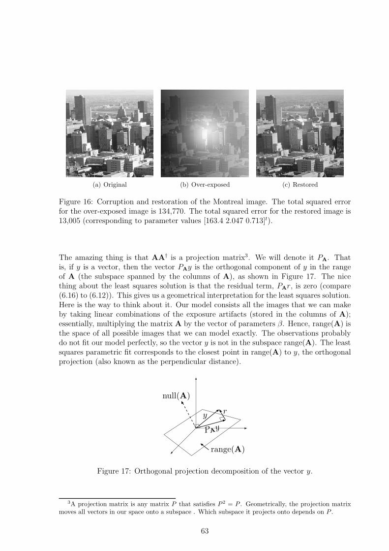
(a) Original (b) Over-exposed (c) Restored
Figure 16: Corruption and restoration of the Montreal image. The total squared errorfor the over-exposed image is 134,770. The total squared error for the restored image is13,005 (corresponding to parameter values [163.4 2.047 0.713]t).
The amazing thing is that AA† is a projection matrix3. We will denote it PA. Thatis, if y is a vector, then the vector PAy is the orthogonal component of y in the rangeof A (the subspace spanned by the columns of A), as shown in Figure 17. The nicething about the least squares solution is that the residual term, PAr, is zero (compare(6.16) to (6.12)). This gives us a geometrical interpretation for the least squares solution.Here is the way to think about it. Our model consists all the images that we can makeby taking linear combinations of the exposure artifacts (stored in the columns of A);essentially, multiplying the matrix A by the vector of parameters β. Hence, range(A) isthe space of all possible images that we can model exactly. The observations probablydo not fit our model perfectly, so the vector y is not in the subspace range(A). The leastsquares parametric fit corresponds to the closest point in range(A) to y, the orthogonalprojection (also known as the perpendicular distance).
null(A)
range(A)
yr
PAy
Figure 17: Orthogonal projection decomposition of the vector y.
3A projection matrix is any matrix P that satisfies P 2 = P . Geometrically, the projection matrixmoves all vectors in our space onto a subspace . Which subspace it projects onto depends on P .
63
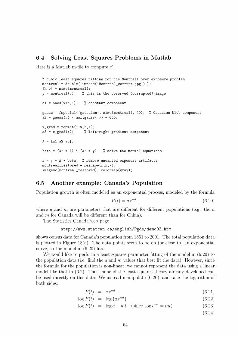
6.4 Solving Least Squares Problems in Matlab
Here is a Matlab m-file to compute β.
% cubic least squares fitting for the Montreal over-exposure problem
montreal = double( imread(’Montreal_corrupt.jpg’) );
[h w] = size(montreal);
y = montreal(:); % this is the observed (corrupted) image
a1 = ones(w*h,1); % constant component
gauss = fspecial(’gaussian’, size(montreal), 40); % Gaussian blob component
a2 = gauss(:) / max(gauss(:)) * 600;
x_grad = repmat(1:w,h,1);
a3 = x_grad(:); % left-right gradient component
A = [a1 a2 a3];
beta = (A’ * A) \ (A’ * y) % solve the normal equations
r = y - A * beta; % remove unwanted exposure artifacts
montreal_restored = reshape(r,h,w);
imagesc(montreal_restored); colormap(gray);
6.5 Another example: Canada’s Population
Population growth is often modeled as an exponential process, modeled by the formula
P (t) = a emt , (6.20)
where a and m are parameters that are different for different populations (e.g. the aand m for Canada will be different than for China).
The Statistics Canada web page
http://www.statcan.ca/english/Pgdb/demo03.htm
shows census data for Canada’s population from 1851 to 2001. The total population datais plotted in Figure 18(a). The data points seem to be on (or close to) an exponentialcurve, so the model in (6.20) fits.
We would like to perform a least squares parameter fitting of the model in (6.20) tothe population data (i.e. find the a and m values that best fit the data). However, sincethe formula for the population is non-linear, we cannot represent the data using a linearmodel like that in (6.2). Thus, none of the least squares theory already developed canbe used directly on this data. We instead manipulate (6.20), and take the logarithm ofboth sides.
P (t) = a emt (6.21)
log P (t) = log(
a emt)
(6.22)
log P (t) = log a + mt (since log emt = mt) (6.23)
(6.24)
64
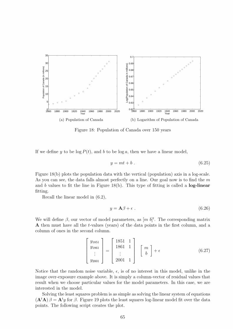
1860 1880 1900 1920 1940 1960 1980 2000 20200
5
10
15
20
25
30
35
Pop
ulat
ion
of C
anad
a (in
mill
ions
)
Year
(a) Population of Canada
1860 1880 1900 1920 1940 1960 1980 2000 20200.62
0.63
0.64
0.65
0.66
0.67
0.68
0.69
0.7
Log(
Pop
ulat
ion
of C
anad
a in
mill
ions
)
Year
(b) Logarithm of Population of Canada
Figure 18: Population of Canada over 150 years
If we define y to be log P (t), and b to be log a, then we have a linear model,
y = mt + b . (6.25)
Figure 18(b) plots the population data with the vertical (population) axis in a log-scale.As you can see, the data falls almost perfectly on a line. Our goal now is to find the mand b values to fit the line in Figure 18(b). This type of fitting is called a log-linearfitting.
Recall the linear model in (6.2),
y = Aβ + ǫ . (6.26)
We will define β, our vector of model parameters, as [m b]t. The corresponding matrixA then must have all the t-values (years) of the data points in the first column, and acolumn of ones in the second column.
y1851
y1861...
y2001
=
1851 11861 1
...2001 1
[
mb
]
+ ǫ (6.27)
Notice that the random noise variable, ǫ, is of no interest in this model, unlike in theimage over-exposure example above. It is simply a column-vector of residual values thatresult when we choose particular values for the model parameters. In this case, we areinterested in the model.
Solving the least squares problem is as simple as solving the linear system of equations(AtA)β = Aty for β. Figure 19 plots the least squares log-linear model fit over the datapoints. The following script creates the plot.
65
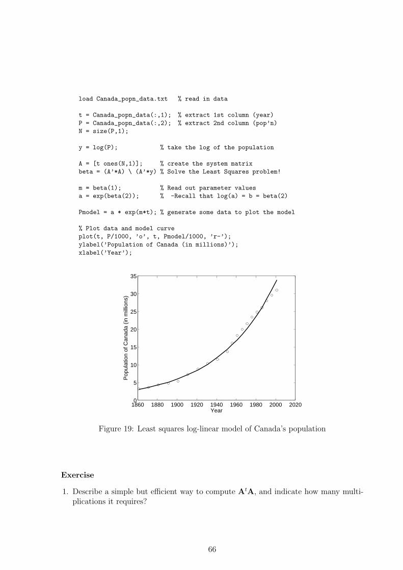
load Canada_popn_data.txt % read in data
t = Canada_popn_data(:,1); % extract 1st column (year)
P = Canada_popn_data(:,2); % extract 2nd column (pop’n)
N = size(P,1);
y = log(P); % take the log of the population
A = [t ones(N,1)]; % create the system matrix
beta = (A’*A) \ (A’*y) % Solve the Least Squares problem!
m = beta(1); % Read out parameter values
a = exp(beta(2)); % -Recall that log(a) = b = beta(2)
Pmodel = a * exp(m*t); % generate some data to plot the model
% Plot data and model curve
plot(t, P/1000, ’o’, t, Pmodel/1000, ’r-’);
ylabel(’Population of Canada (in millions)’);
xlabel(’Year’);
1860 1880 1900 1920 1940 1960 1980 2000 20200
5
10
15
20
25
30
35
Pop
ulat
ion
of C
anad
a (in
mill
ions
)
Year
Figure 19: Least squares log-linear model of Canada’s population
Exercise
1. Describe a simple but efficient way to compute AtA, and indicate how many multi-plications it requires?
66
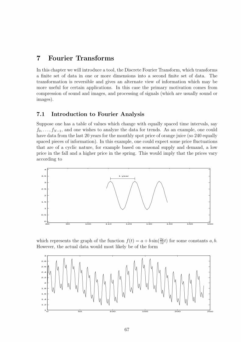
7 Fourier Transforms
In this chapter we will introduce a tool, the Discrete Fourier Transform, which transformsa finite set of data in one or more dimensions into a second finite set of data. Thetransformation is reversible and gives an alternate view of information which may bemore useful for certain applications. In this case the primary motivation comes fromcompression of sound and images, and processing of signals (which are usually sound orimages).
7.1 Introduction to Fourier Analysis
Suppose one has a table of values which change with equally spaced time intervals, sayf0, . . . , fN−1, and one wishes to analyze the data for trends. As an example, one couldhave data from the last 20 years for the monthly spot price of orange juice (so 240 equallyspaced pieces of information). In this example, one could expect some price fluctuationsthat are of a cyclic nature, for example based on seasonal supply and demand, a lowprice in the fall and a higher price in the spring. This would imply that the prices varyaccording to
80 90 100 110 120 130 140 150 160
0
0.5
1
1.5
2
2.5
3
3.5
4
1 year
which represents the graph of the function f(t) = a + b sin(2π12
t) for some constants a, b.However, the actual data would most likely be of the form
0 50 100 150 200 2501
1.2
1.4
1.6
1.8
2
2.2
2.4
2.6
2.8
3
67
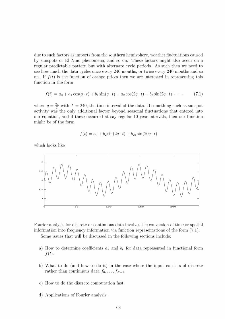
due to such factors as imports from the southern hemisphere, weather fluctuations causedby sunspots or El Nino phenomena, and so on. These factors might also occur on aregular predictable pattern but with alternate cycle periods. As such then we need tosee how much the data cycles once every 240 months, or twice every 240 months and soon. If f(t) is the function of orange prices then we are interested in representing thisfunction in the form
f(t) = a0 + a1 cos(q · t) + b1 sin(q · t) + a2 cos(2q · t) + b2 sin(2q · t) + · · · (7.1)
where q = 2πT
with T = 240, the time interval of the data. If something such as sunspotactivity was the only additional factor beyond seasonal fluctuations that entered intoour equation, and if these occurred at say regular 10 year intervals, then our functionmight be of the form
f(t) = a0 + b2 sin(2q · t) + b20 sin(20q · t)
which looks like
0 50 100 150 200
1
1.5
2
2.5
3
Fourier analysis for discrete or continuous data involves the conversion of time or spatialinformation into frequency information via function representations of the form (7.1).
Some issues that will be discussed in the following sections include:
a) How to determine coefficients ak and bk for data represented in functional formf(t).
b) What to do (and how to do it) in the case where the input consists of discreterather than continuous data f0, . . . , fN−1.
c) How to do the discrete computation fast.
d) Applications of Fourier analysis.
68
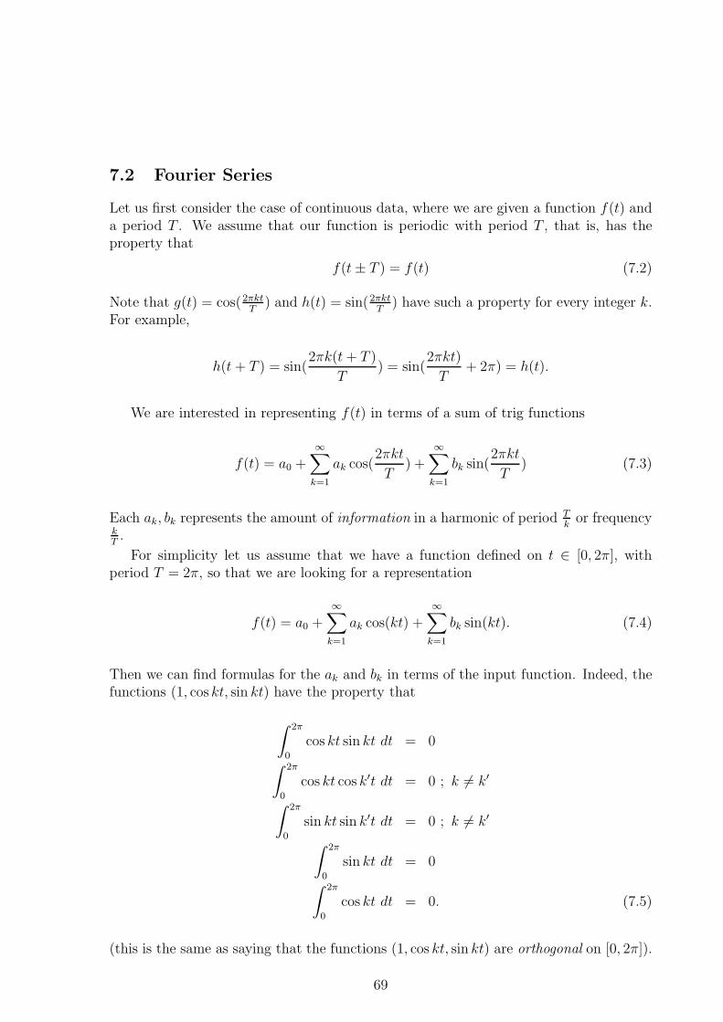
7.2 Fourier Series
Let us first consider the case of continuous data, where we are given a function f(t) anda period T . We assume that our function is periodic with period T , that is, has theproperty that
f(t± T ) = f(t) (7.2)
Note that g(t) = cos(2πktT
) and h(t) = sin(2πktT
) have such a property for every integer k.For example,
h(t + T ) = sin(2πk(t + T )
T) = sin(
2πkt)
T+ 2π) = h(t).
We are interested in representing f(t) in terms of a sum of trig functions
f(t) = a0 +∞∑
k=1
ak cos(2πkt
T) +
∞∑
k=1
bk sin(2πkt
T) (7.3)
Each ak, bk represents the amount of information in a harmonic of period Tk
or frequencykT.
For simplicity let us assume that we have a function defined on t ∈ [0, 2π], withperiod T = 2π, so that we are looking for a representation
f(t) = a0 +∞∑
k=1
ak cos(kt) +∞∑
k=1
bk sin(kt). (7.4)
Then we can find formulas for the ak and bk in terms of the input function. Indeed, thefunctions (1, cos kt, sin kt) have the property that
∫ 2π
0
cos kt sin kt dt = 0
∫ 2π
0
cos kt cos k′t dt = 0 ; k 6= k′
∫ 2π
0
sin kt sin k′t dt = 0 ; k 6= k′
∫ 2π
0
sin kt dt = 0
∫ 2π
0
cos kt dt = 0. (7.5)
(this is the same as saying that the functions (1, cos kt, sin kt) are orthogonal on [0, 2π]).
69
From equations (7.4-7.5) we can determine the coefficients ak, bk.
a0 =
∫ 2π
0
f(t) dt
2π
ak =
∫ 2π
0
f(t) cos kt dt
∫ 2π
0
cos2 kt dt
bk =
∫ 2π
0
f(t) sin kt dt
∫ 2π
0
sin2 kt dt
(7.6)
For example, a formula for aℓ is determined by multiplying both sides of equation (7.4)by cos(ℓt), integrating both sides from 0 to 2π and then taking the integral inside thesummations to be done on a term by term basis. This gives
∫ 2π
0
f(t) cos(ℓt)dt =
∫ 2π
0
a0 cos(ℓt)dt+
∞∑
k=1
∫ 2π
0
ak cos(kt) cos(ℓt)dt+
∞∑
k=1
∫ 2π
0
bk sin(kt) cos(ℓt)dt.
so∫ 2π
0
f(t) cos(ℓt)dt = aℓ
∫ 2π
0
cos(ℓt) cos(ℓt)dt = aℓ · π
and hence our formula for aℓ.We can write the Fourier series (7.4) more compactly if we use Euler’s formula:
ei·θ = cos(θ) + i sin(θ) (7.7)
where i =√−1, something which will become particularly convenient when we consider
the discrete case. Using
e−i·θ = cos(θ)− i sin(θ)
we get that
cos(θ) =ei·θ + e−i·θ
2and sin(θ) =
ei·θ − e−i·θ
2i.
Consequently, we can write
f(t) =
∞∑
k=−∞
ckeikt (7.8)
where ck are in general now complex numbers. The correspondence with the ck and theak, bk of representation (7.3) is given by
c0 = a0, ck =ak
2− i · bk
2and c−k =
ak
2+ i · bk
2for k > 0.
70
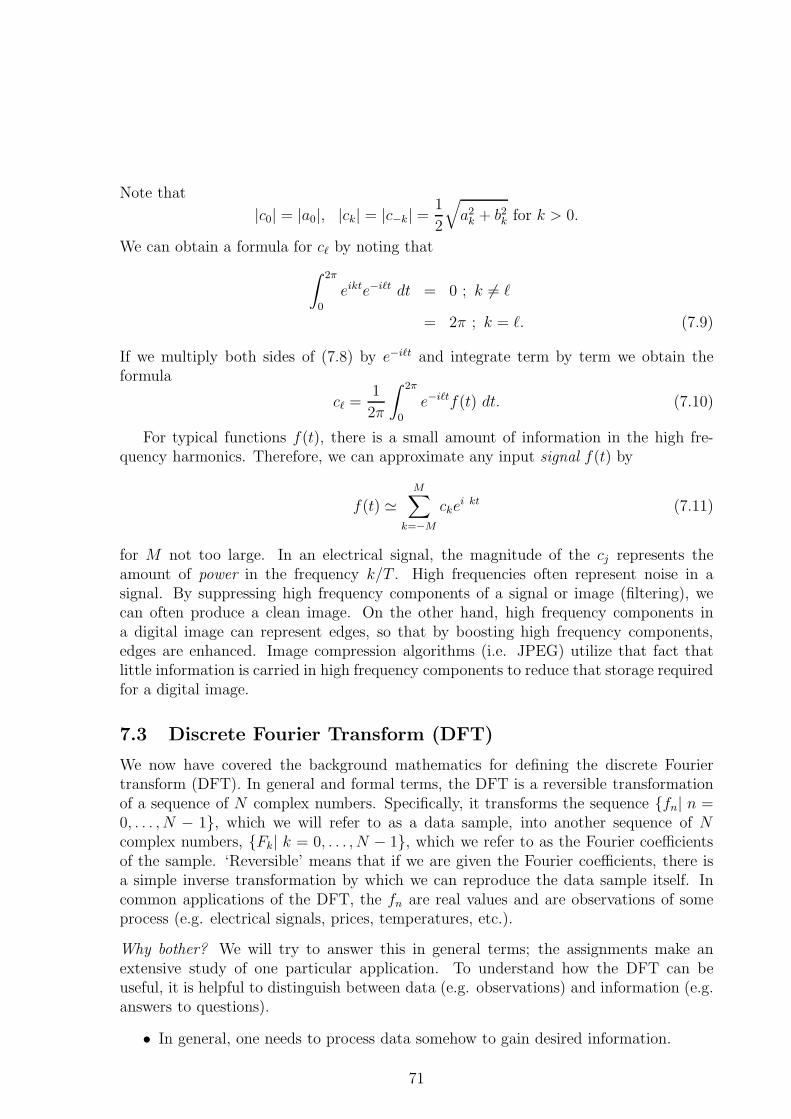
Note that
|c0| = |a0|, |ck| = |c−k| =1
2
√
a2k + b2
k for k > 0.
We can obtain a formula for cℓ by noting that
∫ 2π
0
eikte−iℓt dt = 0 ; k 6= ℓ
= 2π ; k = ℓ. (7.9)
If we multiply both sides of (7.8) by e−iℓt and integrate term by term we obtain theformula
cℓ =1
2π
∫ 2π
0
e−iℓtf(t) dt. (7.10)
For typical functions f(t), there is a small amount of information in the high fre-quency harmonics. Therefore, we can approximate any input signal f(t) by
f(t) ≃M∑
k=−M
ckei kt (7.11)
for M not too large. In an electrical signal, the magnitude of the cj represents theamount of power in the frequency k/T . High frequencies often represent noise in asignal. By suppressing high frequency components of a signal or image (filtering), wecan often produce a clean image. On the other hand, high frequency components ina digital image can represent edges, so that by boosting high frequency components,edges are enhanced. Image compression algorithms (i.e. JPEG) utilize that fact thatlittle information is carried in high frequency components to reduce that storage requiredfor a digital image.
7.3 Discrete Fourier Transform (DFT)
We now have covered the background mathematics for defining the discrete Fouriertransform (DFT). In general and formal terms, the DFT is a reversible transformationof a sequence of N complex numbers. Specifically, it transforms the sequence {fn| n =0, . . . , N − 1}, which we will refer to as a data sample, into another sequence of Ncomplex numbers, {Fk| k = 0, . . . , N − 1}, which we refer to as the Fourier coefficientsof the sample. ‘Reversible’ means that if we are given the Fourier coefficients, there isa simple inverse transformation by which we can reproduce the data sample itself. Incommon applications of the DFT, the fn are real values and are observations of someprocess (e.g. electrical signals, prices, temperatures, etc.).
Why bother? We will try to answer this in general terms; the assignments make anextensive study of one particular application. To understand how the DFT can beuseful, it is helpful to distinguish between data (e.g. observations) and information (e.g.answers to questions).
• In general, one needs to process data somehow to gain desired information.
71
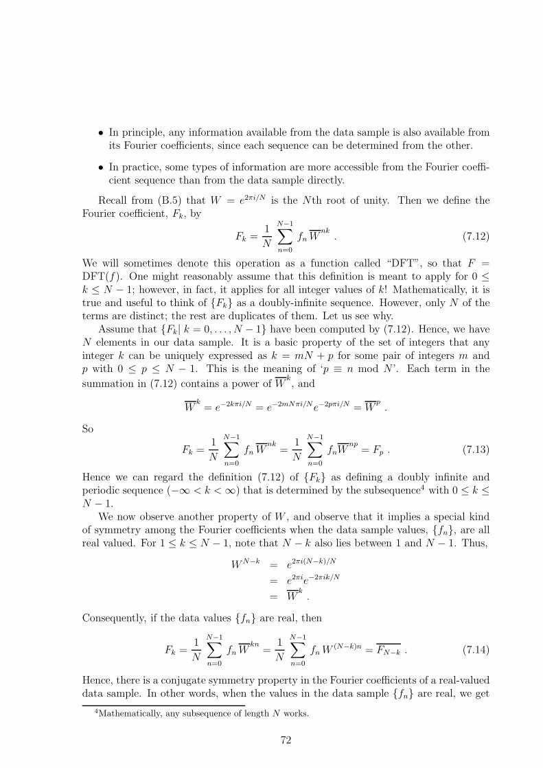
• In principle, any information available from the data sample is also available fromits Fourier coefficients, since each sequence can be determined from the other.
• In practice, some types of information are more accessible from the Fourier coeffi-cient sequence than from the data sample directly.
Recall from (B.5) that W = e2πi/N is the Nth root of unity. Then we define theFourier coefficient, Fk, by
Fk =1
N
N−1∑
n=0
fn Wnk
. (7.12)
We will sometimes denote this operation as a function called “DFT”, so that F =DFT(f). One might reasonably assume that this definition is meant to apply for 0 ≤k ≤ N − 1; however, in fact, it applies for all integer values of k! Mathematically, it istrue and useful to think of {Fk} as a doubly-infinite sequence. However, only N of theterms are distinct; the rest are duplicates of them. Let us see why.
Assume that {Fk| k = 0, . . . , N − 1} have been computed by (7.12). Hence, we haveN elements in our data sample. It is a basic property of the set of integers that anyinteger k can be uniquely expressed as k = mN + p for some pair of integers m andp with 0 ≤ p ≤ N − 1. This is the meaning of ‘p ≡ n mod N ’. Each term in the
summation in (7.12) contains a power of Wk, and
Wk
= e−2kπi/N = e−2mNπi/Ne−2pπi/N = Wp
.
So
Fk =1
N
N−1∑
n=0
fn Wnk
=1
N
N−1∑
n=0
fnWnp
= Fp . (7.13)
Hence we can regard the definition (7.12) of {Fk} as defining a doubly infinite andperiodic sequence (−∞ < k <∞) that is determined by the subsequence4 with 0 ≤ k ≤N − 1.
We now observe another property of W , and observe that it implies a special kindof symmetry among the Fourier coefficients when the data sample values, {fn}, are allreal valued. For 1 ≤ k ≤ N − 1, note that N − k also lies between 1 and N − 1. Thus,
W N−k = e2πi(N−k)/N
= e2πie−2πik/N
= Wk
.
Consequently, if the data values {fn} are real, then
Fk =1
N
N−1∑
n=0
fn Wkn
=1
N
N−1∑
n=0
fn W (N−k)n = FN−k . (7.14)
Hence, there is a conjugate symmetry property in the Fourier coefficients of a real-valueddata sample. In other words, when the values in the data sample {fn} are real, we get
4Mathematically, any subsequence of length N works.
72
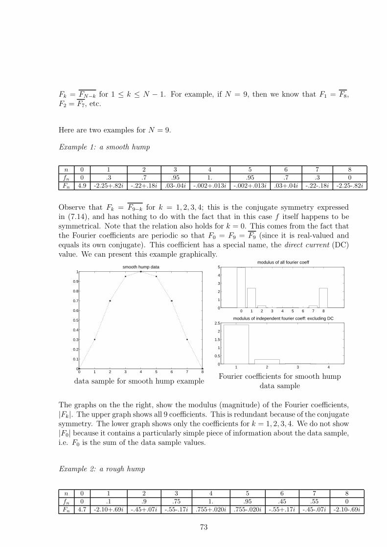
Fk = FN−k for 1 ≤ k ≤ N − 1. For example, if N = 9, then we know that F1 = F8,F2 = F7, etc.
Here are two examples for N = 9.
Example 1: a smooth hump
n 0 1 2 3 4 5 6 7 8fn 0 .3 .7 .95 1. .95 .7 .3 0Fn 4.9 -2.25+.82i -.22+.18i .03-.04i -.002+.013i -.002+.013i .03+.04i -.22-.18i -2.25-.82i
Observe that Fk = F9−k for k = 1, 2, 3, 4; this is the conjugate symmetry expressedin (7.14), and has nothing to do with the fact that in this case f itself happens to besymmetrical. Note that the relation also holds for k = 0. This comes from the fact thatthe Fourier coefficients are periodic so that F0 = F9 = F9 (since it is real-valued andequals its own conjugate). This coefficient has a special name, the direct current (DC)value. We can present this example graphically.
0 1 2 3 4 5 6 7 80
0.1
0.2
0.3
0.4
0.5
0.6
0.7
0.8
0.9
1smooth hump data
data sample for smooth hump example
0 1 2 3 4 5 6 7 80
1
2
3
4
5 modulus of all fourier coeff
1 2 3 40
0.5
1
1.5
2
2.5 modulus of independent fourier coeff: excluding DC
Fourier coefficients for smooth humpdata sample
The graphs on the the right, show the modulus (magnitude) of the Fourier coefficients,|Fk|. The upper graph shows all 9 coefficients. This is redundant because of the conjugatesymmetry. The lower graph shows only the coefficients for k = 1, 2, 3, 4. We do not show|F0| because it contains a particularly simple piece of information about the data sample,i.e. F0 is the sum of the data sample values.
Example 2: a rough hump
n 0 1 2 3 4 5 6 7 8fn 0 .1 .9 .75 1. .95 .45 .55 0Fn 4.7 -2.10+.69i -.45+.07i -.55-.17i .755+.020i .755-.020i -.55+.17i -.45-.07i -2.10-.69i
73
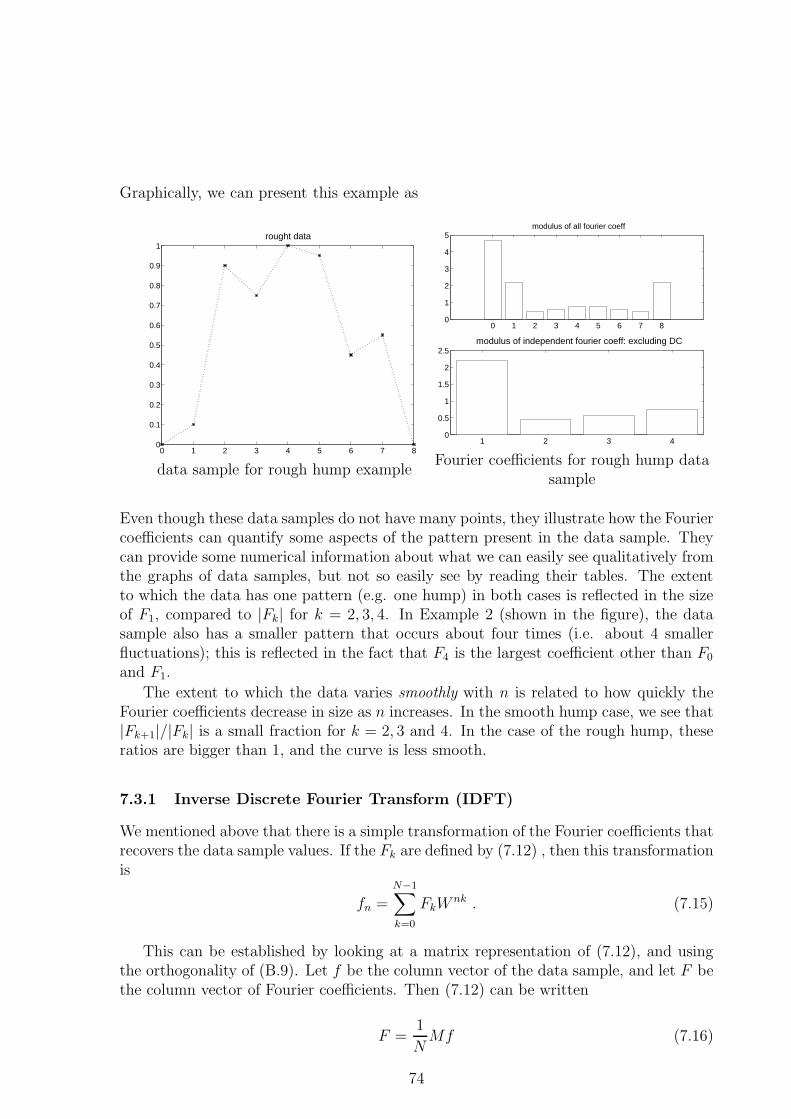
Graphically, we can present this example as
0 1 2 3 4 5 6 7 80
0.1
0.2
0.3
0.4
0.5
0.6
0.7
0.8
0.9
1rought data
data sample for rough hump example
0 1 2 3 4 5 6 7 80
1
2
3
4
5 modulus of all fourier coeff
1 2 3 40
0.5
1
1.5
2
2.5 modulus of independent fourier coeff: excluding DC
Fourier coefficients for rough hump datasample
Even though these data samples do not have many points, they illustrate how the Fouriercoefficients can quantify some aspects of the pattern present in the data sample. Theycan provide some numerical information about what we can easily see qualitatively fromthe graphs of data samples, but not so easily see by reading their tables. The extentto which the data has one pattern (e.g. one hump) in both cases is reflected in the sizeof F1, compared to |Fk| for k = 2, 3, 4. In Example 2 (shown in the figure), the datasample also has a smaller pattern that occurs about four times (i.e. about 4 smallerfluctuations); this is reflected in the fact that F4 is the largest coefficient other than F0
and F1.
The extent to which the data varies smoothly with n is related to how quickly theFourier coefficients decrease in size as n increases. In the smooth hump case, we see that|Fk+1|/|Fk| is a small fraction for k = 2, 3 and 4. In the case of the rough hump, theseratios are bigger than 1, and the curve is less smooth.
7.3.1 Inverse Discrete Fourier Transform (IDFT)
We mentioned above that there is a simple transformation of the Fourier coefficients thatrecovers the data sample values. If the Fk are defined by (7.12) , then this transformationis
fn =N−1∑
k=0
FkWnk . (7.15)
This can be established by looking at a matrix representation of (7.12), and usingthe orthogonality of (B.9). Let f be the column vector of the data sample, and let F bethe column vector of Fourier coefficients. Then (7.12) can be written
F =1
NMf (7.16)
74
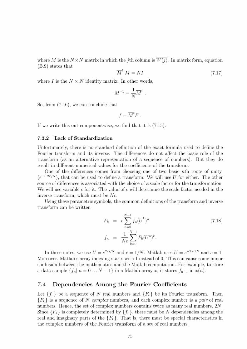
where M is the N×N matrix in which the jth column is W (j). In matrix form, equation(B.9) states that
MtM = NI (7.17)
where I is the N ×N identity matrix. In other words,
M−1 =1
NM
t.
So, from (7.16), we can conclude that
f = MtF .
If we write this out componentwise, we find that it is (7.15).
7.3.2 Lack of Standardization
Unfortunately, there is no standard definition of the exact formula used to define theFourier transform and its inverse. The differences do not affect the basic role of thetransform (as an alternative representation of a sequence of numbers). But they doresult in different numerical values for the coefficients of the transform.
One of the differences comes from choosing one of two basic nth roots of unity,(e±i 2π/N), that can be used to define a transform. We will use U for either. The othersource of differences is associated with the choice of a scale factor for the transformation.We will use variable c for it. The value of c will determine the scale factor needed in theinverse transform, which must be Nc.
Using these parametric symbols, the common definitions of the transform and inversetransform can be written
Fk = cN−1∑
n=0
fn(Uk)n (7.18)
fn =1
Nc
N−1∑
k=0
Fk(Un)k.
In these notes, we use U = e2πi/N and c = 1/N . Matlab uses U = e−2πi/N and c = 1.Moreover, Matlab’s array indexing starts with 1 instead of 0. This can cause some minorconfusion between the mathematics and the Matlab computation. For example, to storea data sample {fn| n = 0 . . .N − 1} in a Matlab array x, it stores fn−1 in x(n).
7.4 Dependencies Among the Fourier Coefficients
Let {fn} be a sequence of N real numbers and {Fk} be its Fourier transform. Then{Fk} is a sequence of N complex numbers, and each complex number is a pair of realnumbers. Hence, the set of complex numbers contains twice as many real numbers, 2N .Since {Fk} is completely determined by {fn}, there must be N dependencies among thereal and imaginary parts of the {Fk}. That is, there must be special characteristics inthe complex numbers of the Fourier transform of a set of real numbers.
75
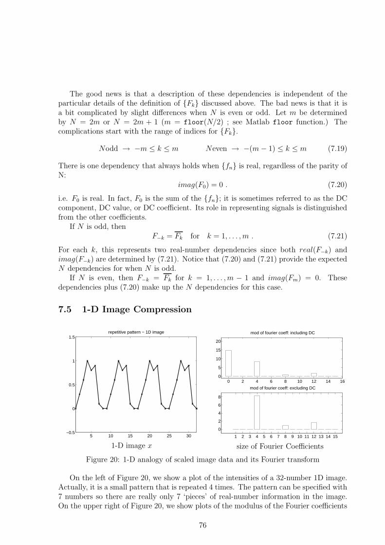
The good news is that a description of these dependencies is independent of theparticular details of the definition of {Fk} discussed above. The bad news is that it isa bit complicated by slight differences when N is even or odd. Let m be determinedby N = 2m or N = 2m + 1 (m = floor(N/2) ; see Matlab floor function.) Thecomplications start with the range of indices for {Fk}.
Nodd → −m ≤ k ≤ m Neven → −(m− 1) ≤ k ≤ m (7.19)
There is one dependency that always holds when {fn} is real, regardless of the parity ofN:
imag(F0) = 0 . (7.20)
i.e. F0 is real. In fact, F0 is the sum of the {fn}; it is sometimes referred to as the DCcomponent, DC value, or DC coefficient. Its role in representing signals is distinguishedfrom the other coefficients.
If N is odd, thenF−k = Fk for k = 1, . . . , m . (7.21)
For each k, this represents two real-number dependencies since both real(F−k) andimag(F−k) are determined by (7.21). Notice that (7.20) and (7.21) provide the expectedN dependencies for when N is odd.
If N is even, then F−k = Fk for k = 1, . . . , m − 1 and imag(Fm) = 0. Thesedependencies plus (7.20) make up the N dependencies for this case.
7.5 1-D Image Compression
5 10 15 20 25 30−0.5
0
0.5
1
1.5repetitive pattern − 1D image
1-D image x
0 2 4 6 8 10 12 14 160
5
10
15
20
mod of fourier coeff: including DC
1 2 3 4 5 6 7 8 9 10 11 12 13 14 15
0
2
4
6
8
mod of fourier coeff: excluding DC
size of Fourier Coefficients
Figure 20: 1-D analogy of scaled image data and its Fourier transform
On the left of Figure 20, we show a plot of the intensities of a 32-number 1D image.Actually, it is a small pattern that is repeated 4 times. The pattern can be specified with7 numbers so there are really only 7 ‘pieces’ of real-number information in the image.On the upper right of Figure 20, we show plots of the modulus of the Fourier coefficients
76
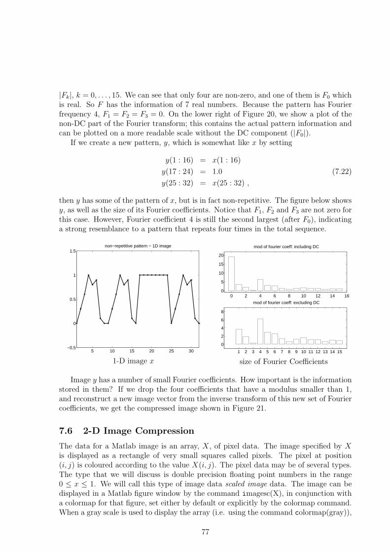
|Fk|, k = 0, . . . , 15. We can see that only four are non-zero, and one of them is F0 whichis real. So F has the information of 7 real numbers. Because the pattern has Fourierfrequency 4, F1 = F2 = F3 = 0. On the lower right of Figure 20, we show a plot of thenon-DC part of the Fourier transform; this contains the actual pattern information andcan be plotted on a more readable scale without the DC component (|F0|).
If we create a new pattern, y, which is somewhat like x by setting
y(1 : 16) = x(1 : 16)
y(17 : 24) = 1.0 (7.22)
y(25 : 32) = x(25 : 32) ,
then y has some of the pattern of x, but is in fact non-repetitive. The figure below showsy, as well as the size of its Fourier coefficients. Notice that F1, F2 and F3 are not zero forthis case. However, Fourier coefficient 4 is still the second largest (after F0), indicatinga strong resemblance to a pattern that repeats four times in the total sequence.
5 10 15 20 25 30−0.5
0
0.5
1
1.5non−repetitive pattern − 1D image
1-D image x
0 2 4 6 8 10 12 14 160
5
10
15
20
mod of fourier coeff: including DC
1 2 3 4 5 6 7 8 9 10 11 12 13 14 15
0
2
4
6
8
mod of fourier coeff: excluding DC
size of Fourier Coefficients
Image y has a number of small Fourier coefficients. How important is the informationstored in them? If we drop the four coefficients that have a modulus smaller than 1,and reconstruct a new image vector from the inverse transform of this new set of Fouriercoefficients, we get the compressed image shown in Figure 21.
7.6 2-D Image Compression
The data for a Matlab image is an array, X, of pixel data. The image specified by Xis displayed as a rectangle of very small squares called pixels. The pixel at position(i, j) is coloured according to the value X(i, j). The pixel data may be of several types.The type that we will discuss is double precision floating point numbers in the range0 ≤ x ≤ 1. We will call this type of image data scaled image data. The image can bedisplayed in a Matlab figure window by the command imagesc(X), in conjunction witha colormap for that figure, set either by default or explicitly by the colormap command.When a gray scale is used to display the array (i.e. using the command colormap(gray)),
77
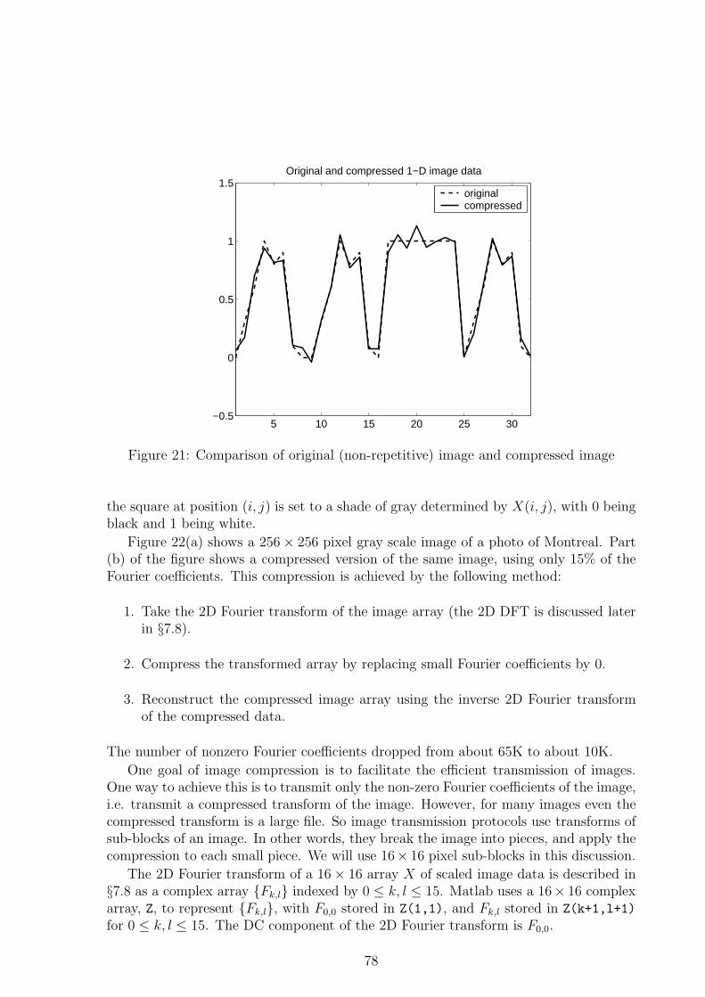
5 10 15 20 25 30−0.5
0
0.5
1
1.5Original and compressed 1−D image data
original compressed
Figure 21: Comparison of original (non-repetitive) image and compressed image
the square at position (i, j) is set to a shade of gray determined by X(i, j), with 0 beingblack and 1 being white.
Figure 22(a) shows a 256× 256 pixel gray scale image of a photo of Montreal. Part(b) of the figure shows a compressed version of the same image, using only 15% of theFourier coefficients. This compression is achieved by the following method:
1. Take the 2D Fourier transform of the image array (the 2D DFT is discussed laterin §7.8).
2. Compress the transformed array by replacing small Fourier coefficients by 0.
3. Reconstruct the compressed image array using the inverse 2D Fourier transformof the compressed data.
The number of nonzero Fourier coefficients dropped from about 65K to about 10K.
One goal of image compression is to facilitate the efficient transmission of images.One way to achieve this is to transmit only the non-zero Fourier coefficients of the image,i.e. transmit a compressed transform of the image. However, for many images even thecompressed transform is a large file. So image transmission protocols use transforms ofsub-blocks of an image. In other words, they break the image into pieces, and apply thecompression to each small piece. We will use 16× 16 pixel sub-blocks in this discussion.
The 2D Fourier transform of a 16× 16 array X of scaled image data is described in§7.8 as a complex array {Fk,l} indexed by 0 ≤ k, l ≤ 15. Matlab uses a 16× 16 complexarray, Z, to represent {Fk,l}, with F0,0 stored in Z(1,1), and Fk,l stored in Z(k+1,l+1)
for 0 ≤ k, l ≤ 15. The DC component of the 2D Fourier transform is F0,0.
78
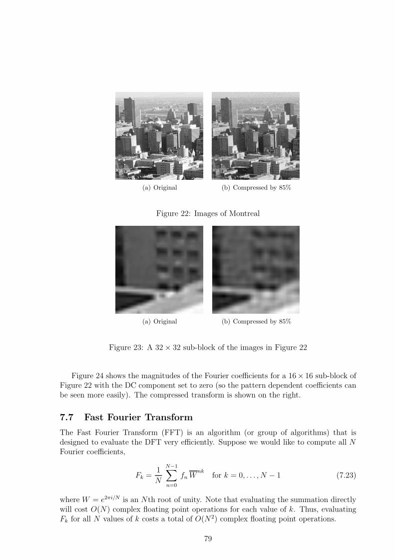
(a) Original (b) Compressed by 85%
Figure 22: Images of Montreal
(a) Original (b) Compressed by 85%
Figure 23: A 32× 32 sub-block of the images in Figure 22
Figure 24 shows the magnitudes of the Fourier coefficients for a 16× 16 sub-block ofFigure 22 with the DC component set to zero (so the pattern dependent coefficients canbe seen more easily). The compressed transform is shown on the right.
7.7 Fast Fourier Transform
The Fast Fourier Transform (FFT) is an algorithm (or group of algorithms) that isdesigned to evaluate the DFT very efficiently. Suppose we would like to compute all NFourier coefficients,
Fk =1
N
N−1∑
n=0
fn Wnk
for k = 0, . . . , N − 1 (7.23)
where W = e2πi/N is an Nth root of unity. Note that evaluating the summation directlywill cost O(N) complex floating point operations for each value of k. Thus, evaluatingFk for all N values of k costs a total of O(N2) complex floating point operations.
79
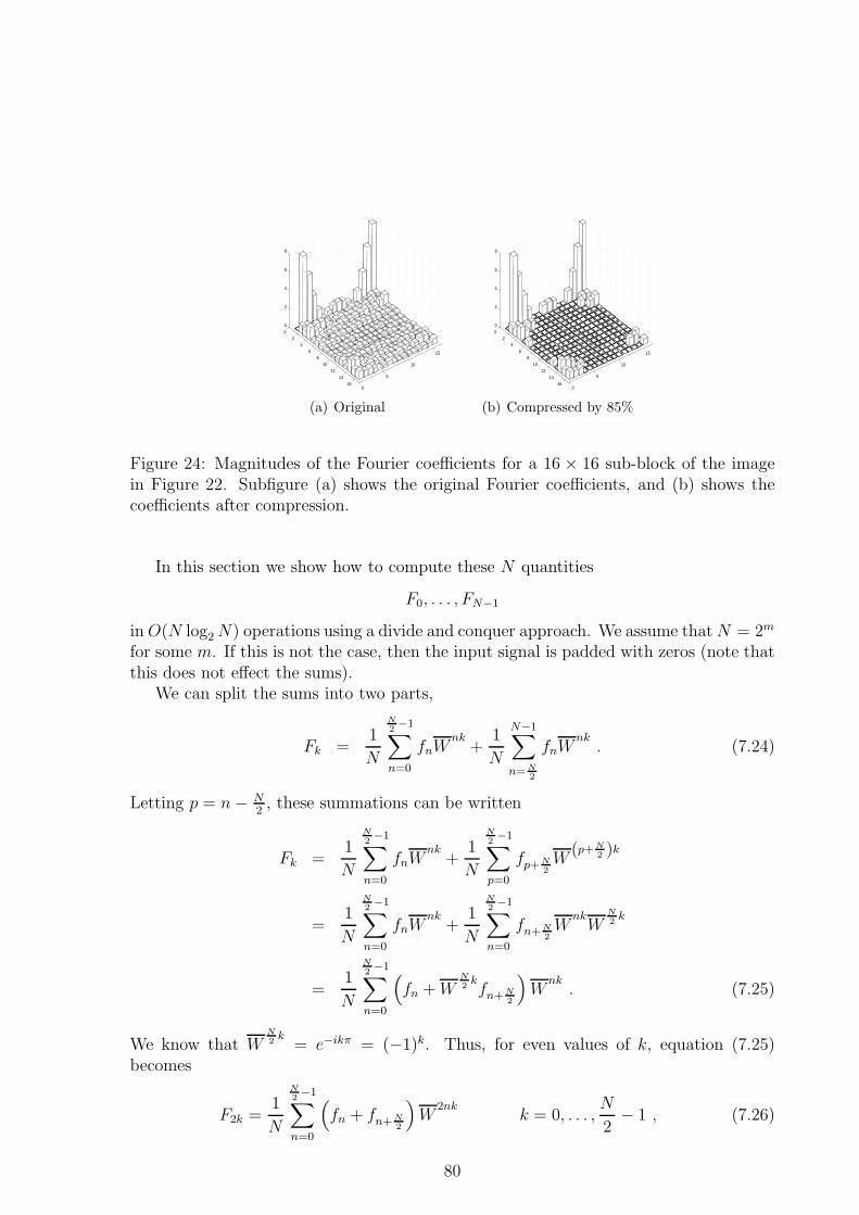
0
5
10
15
02
46
810
1214
16
0
2
4
6
8
(a) Original
0
5
10
15
02
46
810
1214
16
0
2
4
6
8
(b) Compressed by 85%
Figure 24: Magnitudes of the Fourier coefficients for a 16 × 16 sub-block of the imagein Figure 22. Subfigure (a) shows the original Fourier coefficients, and (b) shows thecoefficients after compression.
In this section we show how to compute these N quantities
F0, . . . , FN−1
in O(N log2 N) operations using a divide and conquer approach. We assume that N = 2m
for some m. If this is not the case, then the input signal is padded with zeros (note thatthis does not effect the sums).
We can split the sums into two parts,
Fk =1
N
N2−1∑
n=0
fnWnk
+1
N
N−1∑
n= N2
fnWnk
. (7.24)
Letting p = n− N2, these summations can be written
Fk =1
N
N2−1∑
n=0
fnWnk
+1
N
N2−1∑
p=0
fp+ N2
W(p+ N
2 )k
=1
N
N2−1∑
n=0
fnWnk
+1
N
N2−1∑
n=0
fn+ N2
Wnk
WN2
k
=1
N
N2−1∑
n=0
(
fn + WN2
kfn+ N
2
)
Wnk
. (7.25)
We know that WN2
k= e−ikπ = (−1)k. Thus, for even values of k, equation (7.25)
becomes
F2k =1
N
N2−1∑
n=0
(
fn + fn+ N2
)
W2nk
k = 0, . . . ,N
2− 1 , (7.26)
80
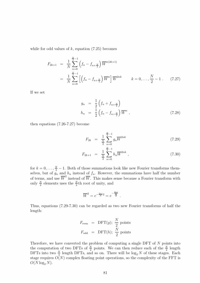
while for odd values of k, equation (7.25) becomes
F2k+1 =1
N
N2−1∑
n=0
(
fn − fn+ N2
)
Wn(2k+1)
=1
N
N2−1∑
n=0
[(
fn − fn+ N2
)
Wn]
W2nk
k = 0, . . . ,N
2− 1 . (7.27)
If we set
gn =1
2
(
fn + fn+ N2
)
hn =1
2
(
fn − fn+ N2
)
Wn
, (7.28)
then equations (7.26-7.27) become
F2k =1N2
N2−1∑
n=0
gnW2nk
(7.29)
F2k+1 =1N2
N2−1∑
n=0
hnW2nk
, (7.30)
for k = 0, . . . , N2− 1. Both of those summations look like new Fourier transforms them-
selves, but of gn and hn instead of fn. However, the summations have half the number
of terms, and use W2
instead of W . This makes sense because a Fourier transform withonly N
2elements uses the N
2th root of unity, and
W2
= e−2πiN
2 = e− 2πi
N2 .
Thus, equations (7.29-7.30) can be regarded as two new Fourier transforms of half thelength:
Feven = DFT(g);N
2points
Fodd = DFT(h);N
2points
Therefore, we have converted the problem of computing a single DFT of N points intothe computation of two DFTs of N
2points. We can then reduce each of the N
2length
DFTs into two N4
length DFTs, and so on. There will be log2 N of these stages. Eachstage requires O(N) complex floating point operations, so the complexity of the FFT isO(N log2 N).
81
7.8 A Two Dimensional FFT
In image processing applications, a grey scale image is represented by a 2D array of greyscale values fn,m, n = 0, . . . , (N − 1) and m = 0, . . . , (M − 1). In this case, the two
dimensional DFT uses two roots of unity, WN = e2πiN and WM = e
2πiM , and is defined as
Fk,l =1
MN
N−1∑
n=0
M−1∑
m=0
fn,mWnk
N Wml
M . (7.31)
Given a function which computes a 1D DFT, how can we use this to compute the 2DDFT above?
We can rewrite equation (7.31) as
Fk,l =1
N
N−1∑
n=0
Wnk
N
[
1
M
M−1∑
m=0
fn,mWml
M
]
=1
N
N−1∑
n=0
Wnk
N Hn,l , (7.32)
where Hn,l = 1M
∑M−1m=0 fn,mW
ml
M . Thus Hn,l can be computed efficiently by taking 1DFFTs of length M of the rows of the input data array. The final computation of Fk,l iscarried out by computing 1D FFTs of length N on the columns of Hn,l. If the complexityof a 1D DFT of length N is CN log2 N , where C is a constant, then the complexity ofa 2D FFT is CNM log2(MN).
Exercises
1. Let {fn}, n = 0, 1, . . . , N − 1, be N samples of a real signal, and N be even.
(a) Show that W−nk + W−(N−n)k = 2 cos(
2πinkN
)
.
(b) Suppose the signal {fn} is an even function (fn = fN−n for n = 1, 2, . . . , N2− 1).
Show that Fk is real.
2. Suppose the signal {fn} is a square signal, defined as
fn =
0 if n = 0, 1, . . . , N4− 1 or n = 3N
4, 3N
4+ 1, . . . , N − 1,
1 if n = N4, N
4+ 1, . . . , 3N
4− 1 .
Show that F2k = 0, k = 1, 2, . . . , N2− 1.
82
8 Dynamic Simulation: Modeling with ODEs
In this section, we will present some small examples of modeling with differential equa-tions. These examples are based on familiar ideas, but typical simulations can requirea very sophisticated understanding of the application area (be it chemistry, finance,electronics, etc.) and usually involves dozens to thousands of equations.
8.1 Single Population Model: How is Canada Growing?
It is common to measure populations in thousands of individuals (Kpersons). Let ususe the symbol Pt for a population at time t in years. For example, if the population ofCanada in the year 2000 was about 30,750,000, then we write P2000 ≈ 30, 750.See http://www.statcan.ca/start.html for the data on the Canadian population usedin this section.
A human population in a fixed geographic region changes in size by
• natural regeneration by the net effects of births and deaths
• net immigration (immigration minus emigration)
Let G denote the natural regeneration rate; the conventional units for G is “eventsper Kpersons per year”, usually written “events/(Kpersons-year)” (that’s a dash, not aminus sign). Average event rates for Canada in 1999-2000 were:
birth rate = 10.9 (i.e. 109 babies per 10,000 persons per year)
death rate = 7.5.
The net regeneration effect is the birth rate minus the death rate, so G ≈ 3.4. Thenumber of immigrants arriving in Canada in 1999-2000 was about 204K. Stats Canadadoes not provide a recent figure for emigration; but it does provide data averagingabout 50Kpersons/year for 1991-1996. So letting I be the net immigration rate, we canestimate I ≈ 155 Kpersons/year.
To simplify the move from this data to mathematical models of population evolution,we make the BIG assumptions that G and I are constant over time. For modelingpurposes, we need the net regeneration rate in units of Kevents per Kpersons per year;not in the customary census data units of events/(Kpersons-year) quoted above. Solet r = G/1000 be this rate in the units of Kevents/(Kpersons-year); i.e. for Canadar ≈ .0034. Then our conceptual model of population change from time t to time t + τcan be written
Pt+τ ≈ Pt + rPtτ + Iτ . (8.1)
These ideas lead us to two closely related mathematical models for predicting populationevolution from a known starting population Pt0 at a given time t0
• a difference equation based model
• a differential equation based model.
83
8.1.1 Difference Equation Model
Let us pick a fixed interval of years, h. We model the population evolution as a sequence{p(n), n = 0, 1, 2, . . .}, where p(n) is the model’s estimate of Pt0+nh. Given the initialpopulation of p(0) = Pt0 , we can compute p(n+1) from p(n) using
p(n+1) = (1 + rh)p(n) + Ih (8.2)
Solution of (8.2): If we let α = 1 + rh, then (8.2) can be written
p(n+1) = αp(n) + Ih
= α(αp(n−1) + Ih) + Ih
= α2(αp(n−2) + Ih) + (α + 1)Ih
= · · ·
If we continue this process, each time substituting p(k) with(
αp(k−1) + Ih)
, we eventually
get down to p(0), and we can write
p(k) = αkp(0) +αk − 1
α− 1Ih
= αk
(
p(0) +Ih
α− 1
)
− Ih
α− 1
Notice that Ihα−1
= Ir, so
p(k) = (1 + rh)k
(
p(0) +I
r
)
− I
r(8.3)
Note the roles of some of the parameters:
• if r > 0 then p(k) →∞ as k →∞ and the model predicts an unlimited populationgrowth.
• if r < 0 and rh ≥ −1 then p(k) → −Ir
as k →∞ and the model predicts a stable,finite population.
• if r < 0 and rh < −1 then the contribution of (1 + rh)p(n) to p(n+1) is negative, amodel prediction that doesn’t make sense. This is because h is too large for thisnegative r value.
8.1.2 Differential Equation Model
If we return to (8.1), we can rewrite it as 1τ(Pt+τ − Pt) ∼= rPt + I . If we introduce
a continuous function of t, p(t), as a mathematical model for the population at time tthen, letting τ → 0, we see that p(t) must satisfy the differential equation
dp(t)
dt= rp(t) + I . (8.4)
84
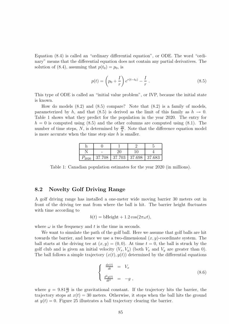
Equation (8.4) is called an “ordinary differential equation”, or ODE. The word “ordi-nary” means that the differential equation does not contain any partial derivatives. Thesolution of (8.4), assuming that p(t0) = p0, is
p(t) =
(
p0 +I
r
)
er(t−t0) − I
r. (8.5)
This type of ODE is called an “initial value problem”, or IVP, because the initial stateis known.
How do models (8.2) and (8.5) compare? Note that (8.2) is a family of models,parameterized by h, and that (8.5) is derived as the limit of this family as h → 0.Table 1 shows what they predict for the population in the year 2020. The entry forh = 0 is computed using (8.5) and the other columns are computed using (8.1). Thenumber of time steps, N , is determined by 20
h. Note that the difference equation model
is more accurate when the time step size h is smaller.
h 0 1 2 5N - 20 10 4
P2020 37.708 37.703 37.698 37.683
Table 1: Canadian population estimates for the year 2020 (in millions).
8.2 Novelty Golf Driving Range
A golf driving range has installed a one-meter wide moving barrier 30 meters out infront of the driving tee mat from where the ball is hit. The barrier height fluctuateswith time according to
b(t) = bHeight + 1.2 cos(2πωt),
where ω is the frequency and t is the time in seconds.
We want to simulate the path of the golf ball. Here we assume that golf balls are hittowards the barrier, and hence we use a two-dimensional (x, y)-coordinate system. Theball starts at the driving tee at (x, y) = (0, 0). At time t = 0, the ball is struck by thegolf club and is given an initial velocity (Vx, Vy) (both Vx and Vy are greater than 0).The ball follows a simple trajectory (x(t), y(t)) determined by the differential equations
dx(t)dt
= Vx
d2y(t)dt2
= −g ,
(8.6)
where g = 9.81ms2
is the gravitational constant. If the trajectory hits the barrier, thetrajectory stops at x(t) = 30 meters. Otherwise, it stops when the ball hits the groundat y(t) = 0. Figure 25 illustrates a ball trajectory clearing the barrier.
85
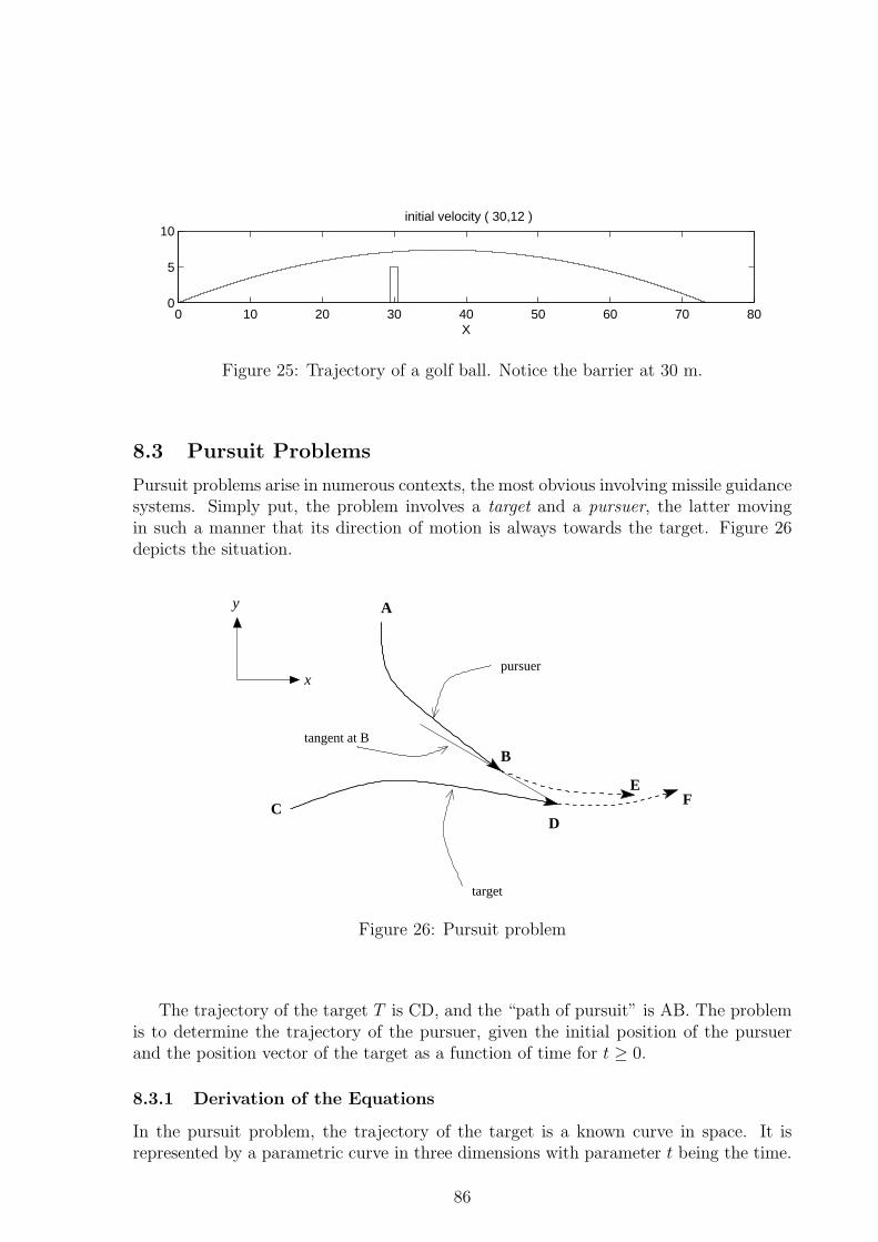
0 10 20 30 40 50 60 70 800
5
10
X
initial velocity ( 30,12 )
Figure 25: Trajectory of a golf ball. Notice the barrier at 30 m.
8.3 Pursuit Problems
Pursuit problems arise in numerous contexts, the most obvious involving missile guidancesystems. Simply put, the problem involves a target and a pursuer, the latter movingin such a manner that its direction of motion is always towards the target. Figure 26depicts the situation.
FE
pursuer
A
CD
B
target
x
y
tangent at B
Figure 26: Pursuit problem
The trajectory of the target T is CD, and the “path of pursuit” is AB. The problemis to determine the trajectory of the pursuer, given the initial position of the pursuerand the position vector of the target as a function of time for t ≥ 0.
8.3.1 Derivation of the Equations
In the pursuit problem, the trajectory of the target is a known curve in space. It isrepresented by a parametric curve in three dimensions with parameter t being the time.
86
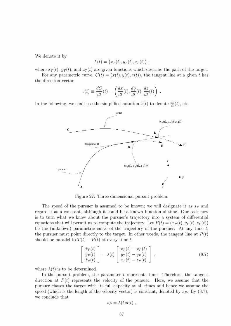
We denote it byT (t) =
(
xT (t), yT (t), zT (t))
,
where xT (t), yT (t), and zT (t) are given functions which describe the path of the target.For any parametric curve, C(t) = (x(t), y(t), z(t)), the tangent line at a given t has
the direction vector
v(t) ≡ dC
dt(t) =
(
dx
dt(t),
dy
dt(t),
dz
dt(t)
)
.
In the following, we shall use the simplified notation x(t) to denote dxdt
(t), etc.
y
z
x
(x (t), y (t), z (t))P P P
pursuer
target
B
A
CD
E Ftangent at B
(x (t), y (t), z (t))T T T
Figure 27: Three-dimensional pursuit problem.
The speed of the pursuer is assumed to be known; we will designate it as sP andregard it as a constant, although it could be a known function of time. Our task nowis to turn what we know about the pursuer’s trajectory into a system of differentialequations that will permit us to compute the trajectory. Let P (t) = (xP (t), yP (t), zP (t))be the (unknown) parametric curve of the trajectory of the pursuer. At any time t,the pursuer must point directly to the target. In other words, the tangent line at P (t)should be parallel to T (t)− P (t) at every time t.
xP (t)yP (t)zP (t)
= λ(t)
xT (t)− xP (t)yT (t)− yP (t)zT (t)− zP (t)
, (8.7)
where λ(t) is to be determined.In the pursuit problem, the parameter t represents time. Therefore, the tangent
direction at P (t) represents the velocity of the pursuer. Here, we assume that thepursuer chases the target with its full capacity at all times and hence we assume thespeed (which is the length of the velocity vector) is constant, denoted by sP . By (8.7),we conclude that
sP = λ(t)d(t) ,
87
where
d(t) =
√
(
xT (t)− xP (t))2
+(
yT (t)− yP (t))2
+(
zT (t)− zP (t))2
. (8.8)
Thus, λ(t) = sP
d(t). Finally, the equations describing the pursuer’s motion are
xP (t)yP (t)zP (t)
=sP
d(t)
xT (t)− xP (t)yT (t)− yP (t)zT (t)− zP (t)
.
If sP is sufficiently large, then the pursuer will intercept the target in finite time.However, in general, the trajectory of the target and the starting positions will determinewhether interception occurs.
8.4 Standard First Order Form for Initial Value Problems
We are going to use computers to approximate the solution of IVPs. In order to do this,we need a standard way to communicate to the computer what the IVP is – what thesystem of ODEs and the initial condition is.
A general system of m ODEs consists of:
- an m-vector valued function, f(t, z) of 1 + m variables, sometimes referred to asthe system dynamics function. The input variable t is the independent variable,while the input vector z represents the current state of the system. We will use theword “state” (or “state variables”) to refer to the (vector of) values that we aremodeling. For example, the state tells us the population at a given time (for thepopulation model), or the position of the pursuer at a given time (for the pursuermodel). Writing out f(t, z) with all its subscripts looks like this:
f1(t, z1, z2, . . . , zm)f2(t, z1, z2, . . . , zm)
...fm(t, z1, z2, . . . , zm)
.
- an m×m matrix, M . In general, M may be a function of t, or even (t, z) like f .In the simple examples presented in these notes, M is the identity matrix so wedon’t need to worry about it.
A solution of the general first order system determined by f(t, z) then is an m-vectorvalued function of time, y(t), that satisfies
Mdy(t)
dt= f(t, y(t)) (8.9)
over some interval of time, t0 ≤ t ≤ tfinal. An initial value problem (IVP) for a systemof the form (8.9) specifies a starting time, t0, and starting state, us. The solution of theinitial value problem, or trajectory, is an m-vector valued function, u(t), that satisfies
88
(8.9) and the initial condition u(t0) = us . In the context of dynamic simulation, itwould be common to say that the system being modeled evolves through the states u(t)with time.
Notice that the dynamics function f takes as input z, the m-vector of state variables.If we assume that M is the identity matrix (and we will), then the function f outputsan m-vector corresponding to the derivatives of these state variables, all listed in thesame order as the input z. So, the dynamics function f is simply a way to calculate theright-hand-sides for the system of ODEs. It tells how things are changing at any giventime and state.
In the preceding subsection, we saw that the novelty golf driving range model usedtwo event functions to determine the end time and status of the simulated drive. Ingeneral, an IVP with m equations in form (8.9) can also have k events that mightoccur during the evolution of u(t). These events are specified using a k-vector valuedfunction, E(t, z). A common specification that the jth event has happened in timeinterval ta < t < tb is that Ej(t, u(t)) changes sign, i.e. Ej(ta, u(ta)) and Ej(tb, u(tb))have opposite signs.
Software for dynamic simulations, including Matlab, require the mathematical model’sequations to be identified as data for the standard first order form described above. Inthis subsection, we identify the mathematical model of each of the dynamic simulationsas an IVP for a system of equations in standard form (8.9). The mass matrix for eachof these cases is the identity matrix; so we will not comment specifically on it.
8.4.1 The single population model
The identification of the single population model for form (8.9) is simple:
• m = 1
• p ∼ y
• f(t, y) = r y + I
• t0 = 2000 ; u(s) = 30750.
8.4.2 The golf driving range
The identification of the novelty golf range model is complicated by the fact that thebasic modeling differential equations in (8.6) include a second derivative of the variables,x(t) and y(t). There is a standard technique of introducing new variables to reduce asystem of ODEs to first order form. This means
• m = 3
• a more complex connection between the variables of the model x and y and thevariables of the form (8.9) y1, y2, y3. The identification is
y1 ∼ x ; y2 ∼ y ; y3 ∼ dy/dt
89
To ensure that y2 and y3 remain consistent with y2 ∼ y and y3 ∼ dy/dt we add theequation dy2(t)/dt = y3(t) to (8.6). The rest of the identification is
f1(t, y) = Vx ; f2(t, y) = y3 ; f3(t, y) = −g (8.10)
and the initial conditions are
t0 = 0 ; u(s) = (0, 0, Vy)t .
The two event functions associated with terminating the golf ball trajectories of thismodel can be written using standard form variables as a 2-vector valued event function,E(t, y)
E1(t, y) = y2
E2(t, y) =
{
1 if |y1 − 30| > 12
or y2 > b(t)−1 otherwise
8.4.3 The pursuit problem
The identification of the pursuit problem as an IVP for the standard form of a first ordersystem of equations is
• m = 3 (for 3-D trajectories)
• y1 ∼ xP ; y2 ∼ yP ; y3 ∼ zP
• t0 = 0 ; u(s) = P (0)
and
f1(t, y) = sP (xT (t)− y1)/dist(t, y)
f2(t, y) = sP (xT (t)− y2)/dist(t, y)
f3(t, y) = sP (xT (t)− y3)/dist(t, y)
The pursuit model also needs an event function to determine if and when the pursuercaptures the target.
8.5 The Matlab ODE Suite
Dynamic simulations based on IVPs in standard form (8.9) are invariably computedusing standard mathematical software. Much of this software is in the public domainand some of the best of it has been incorporated into Matlab. Let u(t) be the solutionof a standard IVP. A program for numerically solving the standard IVP for u (typically)computes two arrays for output:
• a column-vector of Nfinal time values, T = [T1, T2, . . . TNfinal]t, and
90
• an array, Y , containing values for the state variables at the corresponding times.This array has Nfinal rows, each row holding the m-vector of state variables. Thus,the kth row is the solution at time Tk. The computed Y values are approximationsto the solution u in that
Yk,j ≈ uj(Tk) . (8.11)
Matlab has a suite of 7 programs for computing numerical solutions of IVPs. Thesuite has a user interface that is common to all programs. This interface is quite flexibleto accommodate a range of uses from simple to sophisticated. Version 6 of Matlab mademajor changes to this interface (compared to version 5), simplifying it significantly aswell as extending it a small amount.
These notes provide a brief overview of the new interface using some examples. Wedo not intend to provide full technical details. The Matlab help is a reference for themany details of the complete interface5.
8.5.1 The basic form of the ODE suite interface
The basic form of the ODE suite interface assumes that a numerical solution is to becomputed for an IVP of the form shown in equation (8.9) with no mass matrix (moreprecisely, with the mass matrix M = I). The input for the basic form for the interfaceis:
a) the data describing the standard initial value problem based on (8.9) with M = I.This data is the dynamics function f(t, z) and the initial state data t0, us.
b) an explicit final time for the numerical solution, tfinal.
How do we make the dynamics function known to the ODE method? From a pro-gramming language point of view, a natural approach is to make one of the methodparameters a handle (pointer) to a user-defined function. Then the solver could usethis handle to evaluate the function for whatever t and z it likes. This mechanism hasbeen introduced into Matlab in version 6 under the name of function handles. Try help
function handle. Here, we only discuss user-defined functions (stored in .m files), suchas
function res = myFun(t,y)
res = t*t+ y*y
Matlab assumes that the name of the file containing the function is the function namefollowed by the .m extension (myFun.m in the above example)6. The handle of a functionis denoted by adding the @ symbol to the start of the function name, e.g. @myFun.
5In the ‘full product family help’ documentation distributed with Version 6.5, the description isfound in the Contents tree by opening the chain of references MATLAB, Mathematics, DifferentialEquations, Initial Value Problems for ODEs.
6In fact, the function name is defined by the file name (minus the .m extension) regardless of thefunction name in the body of the file.
91
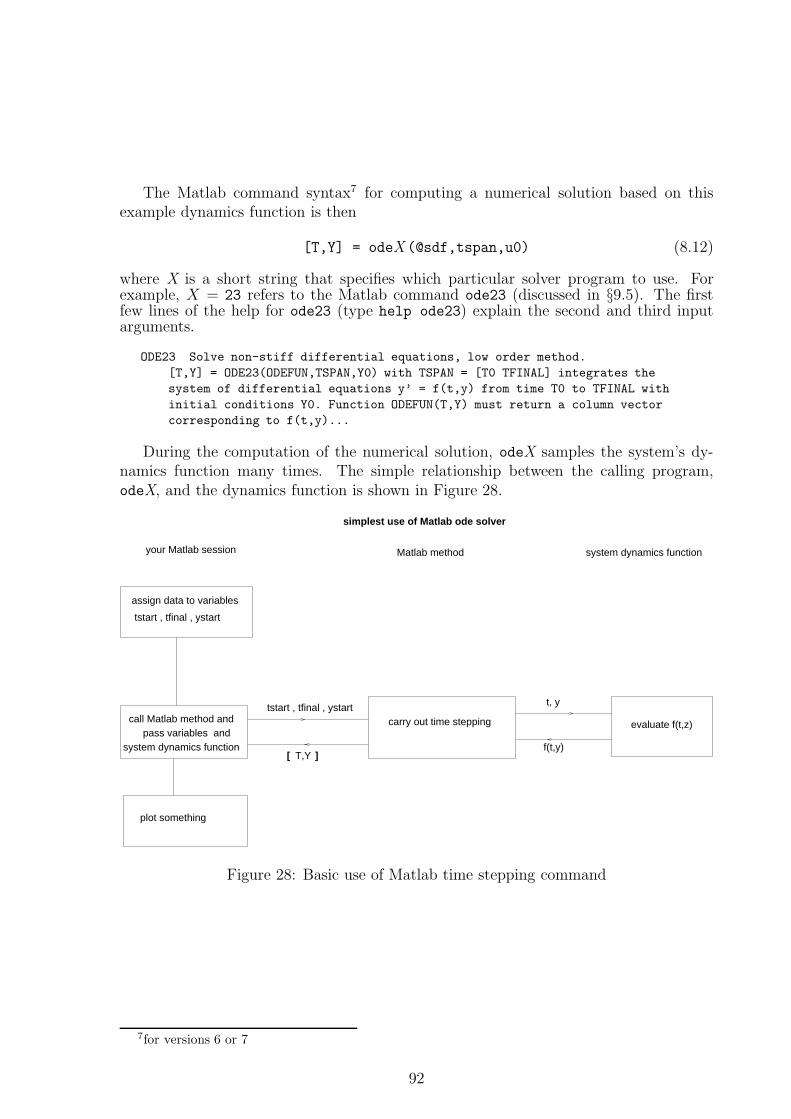
The Matlab command syntax7 for computing a numerical solution based on thisexample dynamics function is then
[T,Y] = odeX (@sdf,tspan,u0) (8.12)
where X is a short string that specifies which particular solver program to use. Forexample, X = 23 refers to the Matlab command ode23 (discussed in §9.5). The firstfew lines of the help for ode23 (type help ode23) explain the second and third inputarguments.
ODE23 Solve non-stiff differential equations, low order method.
[T,Y] = ODE23(ODEFUN,TSPAN,Y0) with TSPAN = [T0 TFINAL] integrates the
system of differential equations y’ = f(t,y) from time T0 to TFINAL with
initial conditions Y0. Function ODEFUN(T,Y) must return a column vector
corresponding to f(t,y)...
During the computation of the numerical solution, odeX samples the system’s dy-namics function many times. The simple relationship between the calling program,odeX, and the dynamics function is shown in Figure 28.
assign data to variables
tstart , tfinal , ystart
plot something
tstart , tfinal , ystart
T,Y
t, y
f(t,y)pass variables
call Matlab method and
[ ]
carry out time stepping evaluate f(t,z)
your Matlab session Matlab method
simplest use of Matlab ode solver
system dynamics function
system dynamics function
and
Figure 28: Basic use of Matlab time stepping command
7for versions 6 or 7
92
8.5.2 Extending the basic form of the Matlab ODE suite interface
The Matlab ODE suite has 17 features, called ‘properties’ in the Matlab documentation,that affect the operation of the ODE solvers. Each property has a default value, but theuser may want to change some of them in order to
a) compute a numerical solution to an IVP for which M 6= I,
b) stop the computation when a certain condition (event) is met, or
c) control the accuracy, or efficiency, of the computation.
How does the ODE suite interface support changing these properties?
The value of each property can be set by a Matlab function called odeset (see help
odeset). This function creates a Matlab internal data structure called an option
structure, recording the desired options. The input arguments for the odeset func-tion are of the form ‘name’, value, specifying a property-name/property-value pair.A user can change any combination of the 17 properties using a single call to odeset;the resulting option structure can then be passed to the appropriate odeX command asthe 4th argument. The values of individual options in the structure can be obtained byusing the Matlab odeget command (not commonly necessary).
A common reason for overriding a property of the ODE suite is that the standardform of the model equations includes a mass matrix, M , that is not the identity matrix.In this case, the Mass property must be overridden. A second reason is the use of eventfunctions, described in the next section. Scenarios involving controlling the accuracyand efficiency will be discussed in §9.5.2.
Explicitly setting the Events property
If an IVP has one, or more, event functions as part of its specification, this is commu-nicated to the ODE suite by appropriately setting the Events property. The value ofthe Events property is a function handle for a user-defined Matlab event function; thedefault is a NULL pointer. The simplest syntax for a Matlab event function is
[val, terminal, direction] = eventFunct(t,z)
If the IVP in question has, say, 3 events in its specification, then the Matlab eventFunct
function of this syntax would return val as a three-vector giving the values of the threeevents.
Suppose we wish to use ode23 to generate a numerical solution to the novelty golfIVP discussed in the preceding section. Communicating the event functions can be donewith the following lines of Matlab:
myOpts = odeset(‘Events’, @golfEvents);
[T,Y,TEvent,YEvent,EventNum] = ode23(@GolfDyn,tspan,u0,myOpts);
93
The first command sets the value of the Events property to the function handle andcreates an option structure named myOpts. In the second command, the option structureis passed to the ode method.
Matlab “help ode23” includes the following description of this command syntax.
[T,Y,TE,YE,IE] = ODE23(ODEFUN,TSPAN,Y0,OPTIONS...) with the ’Events’
property in OPTIONS set to a function EVENTS, solves as above while also
finding where functions of (T,Y), called event functions, are zero. For
each function you specify whether the integration is to terminate at a
zero and whether the direction of the zero crossing matters. These are
the three vectors returned by EVENTS: [VALUE,ISTERMINAL,DIRECTION] =
EVENTS(T,Y). For the I-th event function: VALUE(I) is the value of the
function, ISTERMINAL(I)=1 if the integration is to terminate at a zero of
this event function and 0 otherwise. DIRECTION(I)=0 if all zeros are to
be computed (the default), +1 if only zeros where the event function is
increasing, and -1 if only zeros where the event function is
decreasing. Output TE is a column vector of times at which events
occur. Rows of YE are the corresponding solutions, and indices in vector
IE specify which event occurred.
If the simulation is intended to end at a time determined by an event, then TFINAL
of TSPAN becomes a safety net to ensure the computation eventually terminates.
An example: the novelty golf driving range
We can use this simple model to demonstrate several of the features of the ODE suiteinterface. The dynamics function for this model is given in (8.10). There are two modelparameters in its definition: Vx, the horizontal velocity of the ball, and g, the verticalacceleration due to gravity. The parameter g is a constant, so its value can be hard-codedinto the dynamics function. However, Vx is a key modeling parameter that we want tospecify in our call to odeX (so that we can easily change it). Figure 28 shows that theuser never explicitly calls the dynamics function; the dynamics function is called by theODE solver. Somehow the value of Vx must be passed through to the dynamics function.
There are two ways (at least) to do this. The simplest is to declare Vx as a global
variable both in your session and in the dynamics function code. This has the usualproblems of global variables as programs get larger and more complex.
The second (and better) way is to expand the parameter list of the dynamics function,adding Vx (or some other parameter name) at the end of the default list. So, insteadof the default arguments for the dynamics function (t,y), we have (t,y,Vx). But howdoes odeX know that it should supply a value for this extra parameter when it callsthe dynamics function? Answer: The parameter list of odeX is also extended by oneparameter8. Making Vx a parameter is the preferred program design route for simulationsof any significant size.
Important: Matlab’s implementation has the following quirk that shows up in thegolf driving range example. The parameter list for Matlab event functions must matchthat of dynamics functions. You can see the results in the following Matlab functioncodes for the novelty golf driving range simulation.
8making the parameter list of length at least 5
94
Dynamics Function
function dzdt = golf(t, z, Vx)
% z(1) = x(t)
% z(2) = y(t)
% z(3) = y’(t)
dzdt = [ Vx ; z(3) ; -9.81 ];
Events Function
function [values, halt, dir] = golfEvents(t, z, Vx)
% z(1) = x(t); z(2) = y(t); z(3) = y’(t)
% Vx = horizontal velocity - weird Matlab quirk -
% the dynamics function and the events functions MUST have
% same number of extra parameters. We don’t need Vx here
% but we do in the dynamics function, "golf"
% barrier has average height = bHeight
% centered on fieldSize, and fluctuates by up and down by 1.2 meters
% every 2 seconds (i.e. with frequency 0.5)
f = 0.5; % barrier frequency
fieldSize = 30; % meters
bHeight = 4; % so barrier fluctuates between 2.8 and 5.2 meters
values = [0,0]’;
halt = [1,1]’;
dir = [0,0]’;
% Event 1: the ball hits the ground (the ground is located at z(2)=y=0).
values(1) = z(2); % change of sign (+ to -) indicates event 1
% Event 2: the ball hits the barrier
bDyn = bHeight + 1.2 * cos(2 * pi * f * t); % dynamic barrier height
values(2) = 1;
if ( abs(z(1) - fieldSize) < 0.5 ) && ( z(2) < bDyn )
disp(’inside barrier’)
values(2) = -1;
end;
Matlab session driver script
% set initial velocity imparted by the golfer’s drive here
Vx = 22; Vy = 12; % m/s
disp([’Vx=’ num2str(Vx) ’, Vy=’ num2str(Vy)]);
tspan = [0 5]
initial = [0; 0; Vy]
95

% Vx*h is the horizontal distance travelled in time h.
% Set MaxStep so that Vx*MaxStep = 1, so time stepping can’t
% pass through a 2 meter wide barrier in one step.
options = odeset(’Events’,@golfEvents, ’MaxStep’, 1/Vx);
[t,z] = ode45(@golf,tspan,initial,options,Vx);
N = length(t)
disp(’tfinal, Xfinal, Yfinal’);
disp([t(N),z(N,1), z(N,2)]);
96
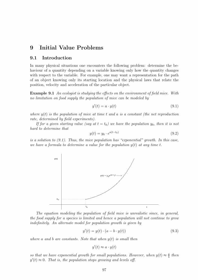
9 Initial Value Problems
9.1 Introduction
In many physical situations one encounters the following problem: determine the be-haviour of a quantity depending on a variable knowing only how the quantity changeswith respect to the variable. For example, one may want a representation for the pathof an object knowing only its starting location and the physical laws that relate theposition, velocity and acceleration of the particular object.
Example 9.1 An ecologist is studying the effects on the environment of field mice. Withno limitation on food supply the population of mice can be modeled by
y′(t) = a · y(t) (9.1)
where y(t) is the population of mice at time t and a is a constant (the net reproductionrate, determined by field experiments).
If for a given starting value (say at t = t0) we have the population y0, then it is nothard to determine that
y(t) = y0 · ea(t−t0) (9.2)
is a solution to (9.1). Thus, the mice population has “exponential” growth. In this case,we have a formula to determine a value for the population y(t) at any time t.
t
y(t)
t0
y0
y(t) = y0ea(t−t
0) −−−>
The equation modeling the population of field mice is unrealistic since, in general,the food supply for a species is limited and hence a population will not continue to growindefinitely. An alternate model for population growth is given by
y′(t) = y(t) · (a− b · y(t)) (9.3)
where a and b are constants. Note that when y(t) is small then
y′(t) ≈ a · y(t)
so that we have exponential growth for small populations. However, when y(t) ≈ ab
theny′(t) ≈ 0. That is, the population stops growing and levels off.
97
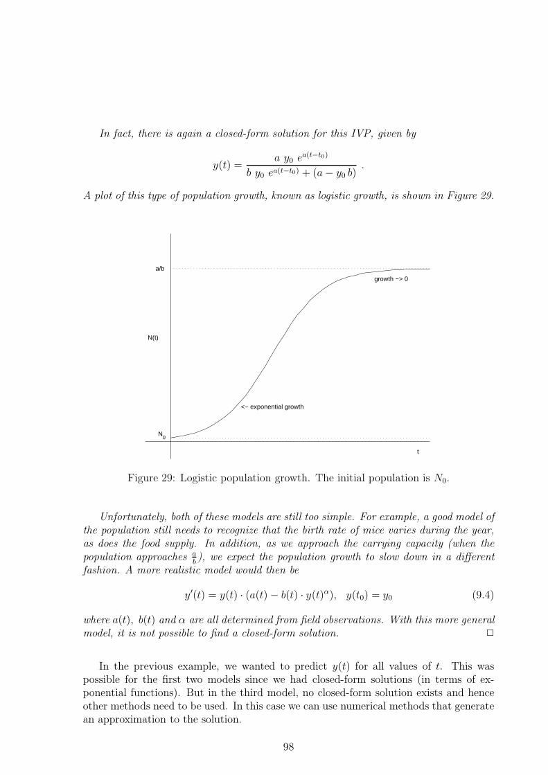
In fact, there is again a closed-form solution for this IVP, given by
y(t) =a y0 ea(t−t0)
b y0 ea(t−t0) + (a− y0 b).
A plot of this type of population growth, known as logistic growth, is shown in Figure 29.
N0
a/b
<− exponential growth
growth −> 0
t
N(t)
Figure 29: Logistic population growth. The initial population is N0.
Unfortunately, both of these models are still too simple. For example, a good model ofthe population still needs to recognize that the birth rate of mice varies during the year,as does the food supply. In addition, as we approach the carrying capacity (when thepopulation approaches a
b), we expect the population growth to slow down in a different
fashion. A more realistic model would then be
y′(t) = y(t) · (a(t)− b(t) · y(t)α), y(t0) = y0 (9.4)
where a(t), b(t) and α are all determined from field observations. With this more generalmodel, it is not possible to find a closed-form solution. 2
In the previous example, we wanted to predict y(t) for all values of t. This waspossible for the first two models since we had closed-form solutions (in terms of ex-ponential functions). But in the third model, no closed-form solution exists and henceother methods need to be used. In this case we can use numerical methods that generatean approximation to the solution.
98
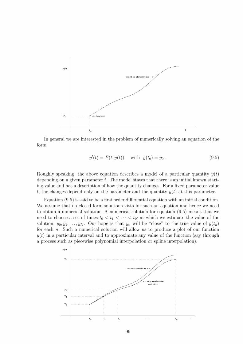
t0
y0 <− known
want to determine −>
t
y(t)
In general we are interested in the problem of numerically solving an equation of theform
y′(t) = F (t, y(t)) with y(t0) = y0 . (9.5)
Roughly speaking, the above equation describes a model of a particular quantity y(t)depending on a given parameter t. The model states that there is an initial known start-ing value and has a description of how the quantity changes. For a fixed parameter valuet, the changes depend only on the parameter and the quantity y(t) at this parameter.
Equation (9.5) is said to be a first order differential equation with an initial condition.We assume that no closed-form solution exists for such an equation and hence we needto obtain a numerical solution. A numerical solution for equation (9.5) means that weneed to choose a set of times t0 < t1 < · · · < tN at which we estimate the value of thesolution, y0, y1, . . . , yN . Our hope is that yn will be “close” to the true value of y(tn)for each n. Such a numerical solution will allow us to produce a plot of our functiony(t) in a particular interval and to approximate any value of the function (say througha process such as piecewise polynomial interpolation or spline interpolation).
t0
y0
t1
y1
t2
y2
... tn
yn
exact solution −>
<− approximate
solution
t
y(t)
99
9.1.1 Other Differential Equations
There are other situations in which one wants to determine a particular set of quantitiesknowing only how those quantities change.
Example 9.2 Let ~P (t) = (x(t), y(t), z(t)) be the coordinates of an airplane, relative to
some starting point. Let the velocity of the airplane ~V (t) be (vx(t), vy(t), vz(t)) and the
components of the acceleration ~A(t) be (ax(t), ay(t), az(t)).An inertial guidance system works by using accelerometers to detect acceleration.
The system then solves the following system of differential equations (in real time)
x′(t) = vx(t), y′(t) = vy(t), z′(t) = vz(t),v′
x(t) = ax(t), v′y(t) = ay(t), v′
z(t) = az(t)(9.6)
where x′(t) = dxdt
, v′x(t) = dvx
dtetc. At t = 0 we know that the airplane is at rest and so
we also have the following initial conditions
(x(0), y(0), z(0)) = (x0, y0, z0) and (vx(0), vy(0), vz(0)) = (0, 0, 0). (9.7)
Equations (9.6) and (9.7) constitute a system of differential equations with an initialcondition. Given the values of the x-, y-, and z-components of acceleration as a functionof time, we can solve these equations to determine the position of the airplane at anytime t. Note that it is crucial to specify the initial condition. 2
Systems of differential equations also appear in such applications as robot controland pipeline leak detection. They also give us a way to look at higher-order equations.
Example 9.3 Consider the 2nd-order linear differential equation given by
y′′(t)− t y′(t) + a y(t) = sin(t), with y(0) = y0, y′(0) = 3.
We can write this equation as a first-order system of linear differential equations withvariables y(t) and z(t) = y′(t) via
y′(t) = z(t)z′(t) = t z(t)− a y(t) + sin(t)
with y(0) = y0 and z(0) = 3.
2
In general, a higher-order differential equation is of the form
y(n)(t) = F (t, y(t), y′(t), . . . , y(n−1)(t)) (9.8)
with initial conditions specified for the first n−1 derivatives at an initial value t0. Againsuch a system can be written as a system of first-order equations with initial conditions.
One can also define systems of partial differential equations where there are quantitiesthat depend on more than on variable. These appear in applications such as animation(for example the water waves in the movie Titanic), design of aircraft, pricing of optionsand hedging in finance, weather prediction and the effect of greenhouse gasses on theenvironment.
100
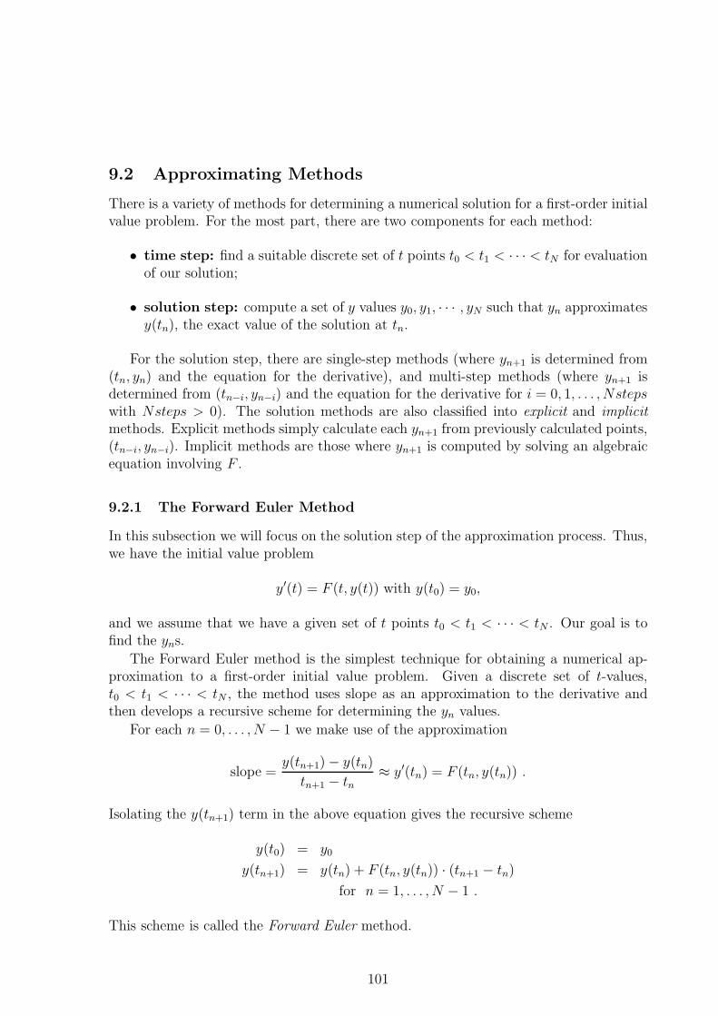
9.2 Approximating Methods
There is a variety of methods for determining a numerical solution for a first-order initialvalue problem. For the most part, there are two components for each method:
• time step: find a suitable discrete set of t points t0 < t1 < · · · < tN for evaluationof our solution;
• solution step: compute a set of y values y0, y1, · · · , yN such that yn approximatesy(tn), the exact value of the solution at tn.
For the solution step, there are single-step methods (where yn+1 is determined from(tn, yn) and the equation for the derivative), and multi-step methods (where yn+1 isdetermined from (tn−i, yn−i) and the equation for the derivative for i = 0, 1, . . . , Nstepswith Nsteps > 0). The solution methods are also classified into explicit and implicitmethods. Explicit methods simply calculate each yn+1 from previously calculated points,(tn−i, yn−i). Implicit methods are those where yn+1 is computed by solving an algebraicequation involving F .
9.2.1 The Forward Euler Method
In this subsection we will focus on the solution step of the approximation process. Thus,we have the initial value problem
y′(t) = F (t, y(t)) with y(t0) = y0,
and we assume that we have a given set of t points t0 < t1 < · · · < tN . Our goal is tofind the yns.
The Forward Euler method is the simplest technique for obtaining a numerical ap-proximation to a first-order initial value problem. Given a discrete set of t-values,t0 < t1 < · · · < tN , the method uses slope as an approximation to the derivative andthen develops a recursive scheme for determining the yn values.
For each n = 0, . . . , N − 1 we make use of the approximation
slope =y(tn+1)− y(tn)
tn+1 − tn≈ y′(tn) = F (tn, y(tn)) .
Isolating the y(tn+1) term in the above equation gives the recursive scheme
y(t0) = y0
y(tn+1) = y(tn) + F (tn, y(tn)) · (tn+1 − tn)
for n = 1, . . . , N − 1 .
This scheme is called the Forward Euler method.
101
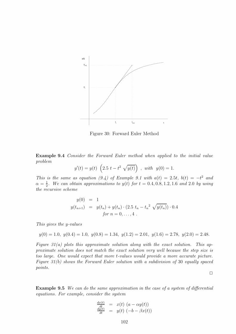
t
y(t)
ti
ti+1
yi
yi+1
Figure 30: Forward Euler Method
Example 9.4 Consider the Forward Euler method when applied to the initial valueproblem
y′(t) = y(t)(
2.5 t− t2√
y(t))
, with y(0) = 1.
This is the same as equation (9.4) of Example 9.1 with a(t) = 2.5t, b(t) = −t2 andα = 1
2. We can obtain approximations to y(t) for t = 0.4, 0.8, 1.2, 1.6 and 2.0 by using
the recursive scheme
y(0) = 1
y(tn+1) = y(tn) + y(tn) · (2.5 tn − tn2√
y(tn)) · 0.4for n = 0, . . . , 4 .
This gives the y-values
y(0) = 1.0, y(0.4) = 1.0, y(0.8) = 1.34, y(1.2) = 2.01, y(1.6) = 2.78, y(2.0) = 2.48.
Figure 31(a) plots this approximate solution along with the exact solution. This ap-proximate solution does not match the exact solution very well because the step size istoo large. One would expect that more t-values would provide a more accurate picture.Figure 31(b) shows the Forward Euler solution with a subdivision of 30 equally spacedpoints.
2
Example 9.5 We can do the same approximation in the case of a system of differentialequations. For example, consider the system
dx(t)dt
= x(t) (a− αy(t))dy(t)
dt= y(t) (−b− βx(t))
102
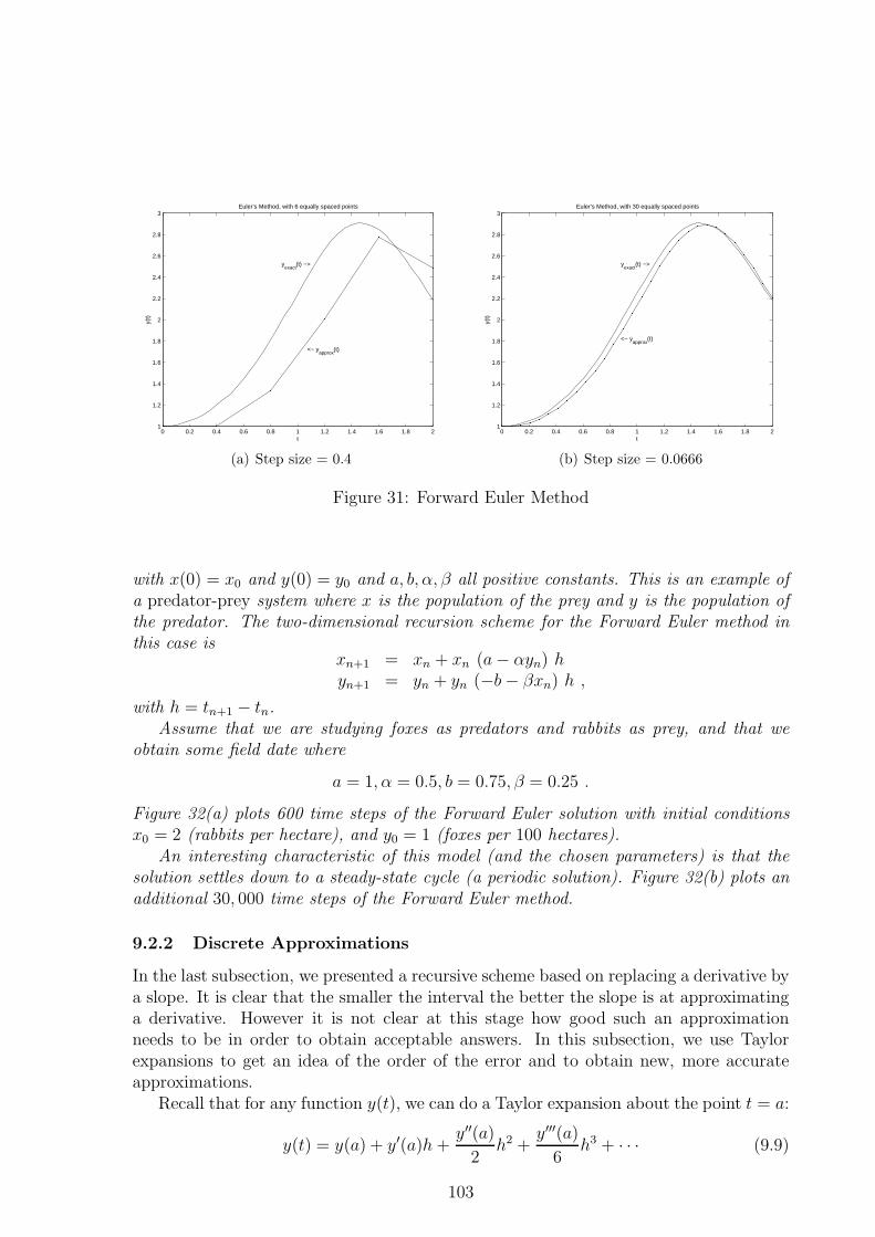
0 0.2 0.4 0.6 0.8 1 1.2 1.4 1.6 1.8 21
1.2
1.4
1.6
1.8
2
2.2
2.4
2.6
2.8
3
t
y(t)
Euler’s Method, with 6 equally spaced points
yexact
(t) −>
<− yapprox
(t)
(a) Step size = 0.4
0 0.2 0.4 0.6 0.8 1 1.2 1.4 1.6 1.8 21
1.2
1.4
1.6
1.8
2
2.2
2.4
2.6
2.8
3
t
y(t)
Euler’s Method, with 30 equally spaced points
yexact
(t) −>
<− yapprox
(t)
(b) Step size = 0.0666
Figure 31: Forward Euler Method
with x(0) = x0 and y(0) = y0 and a, b, α, β all positive constants. This is an example ofa predator-prey system where x is the population of the prey and y is the population ofthe predator. The two-dimensional recursion scheme for the Forward Euler method inthis case is
xn+1 = xn + xn (a− αyn) hyn+1 = yn + yn (−b− βxn) h ,
with h = tn+1 − tn.Assume that we are studying foxes as predators and rabbits as prey, and that we
obtain some field date where
a = 1, α = 0.5, b = 0.75, β = 0.25 .
Figure 32(a) plots 600 time steps of the Forward Euler solution with initial conditionsx0 = 2 (rabbits per hectare), and y0 = 1 (foxes per 100 hectares).
An interesting characteristic of this model (and the chosen parameters) is that thesolution settles down to a steady-state cycle (a periodic solution). Figure 32(b) plots anadditional 30, 000 time steps of the Forward Euler method.
9.2.2 Discrete Approximations
In the last subsection, we presented a recursive scheme based on replacing a derivative bya slope. It is clear that the smaller the interval the better the slope is at approximatinga derivative. However it is not clear at this stage how good such an approximationneeds to be in order to obtain acceptable answers. In this subsection, we use Taylorexpansions to get an idea of the order of the error and to obtain new, more accurateapproximations.
Recall that for any function y(t), we can do a Taylor expansion about the point t = a:
y(t) = y(a) + y′(a)h +y′′(a)
2h2 +
y′′′(a)
6h3 + · · · (9.9)
103
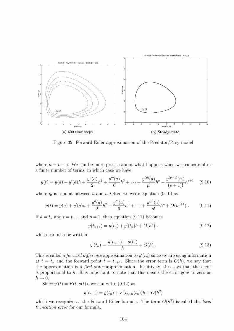
0 1 2 3 4 5 6 7 8 9 100
1
2
3
4
5
6Predator−Prey Model for Foxes and Rabbits: ∆ t = 0.05
Rabbits (x)
Fox
es (
y)
(x0,y
0)
(a) 600 time steps
0 1 2 3 4 5 6 7 8 9 100
1
2
3
4
5
6Predator−Prey Model for Foxes and Rabbits: ∆ t = 0.001
Rabbits (x)
Fox
es (
y)
(x0,y
0)
(b) Steady-state
Figure 32: Forward Euler approximation of the Predator/Prey model
where h = t − a. We can be more precise about what happens when we truncate aftera finite number of terms, in which case we have
y(t) = y(a) + y′(a)h +y′′(a)
2h2 +
y′′′(a)
6h3 + · · ·+ y(p)(a)
p!hp +
y(p+1)(ηt)
(p + 1)!hp+1 (9.10)
where ηt is a point between a and t. Often we write equation (9.10) as
y(t) = y(a) + y′(a)h +y′′(a)
2h2 +
y′′′(a)
6h3 + · · ·+ y(p)(a)
p!hp + O(hp+1) . (9.11)
If a = tn and t = tn+1 and p = 1, then equation (9.11) becomes
y(tn+1) = y(tn) + y′(tn)h + O(h2) . (9.12)
which can also be written
y′(tn) =y(tn+1)− y(tn)
h+ O(h) . (9.13)
This is called a forward difference approximation to y′(tn) since we are using informationat t = tn and the forward point t = tn+1. Since the error term is O(h), we say thatthe approximation is a first-order approximation. Intuitively, this says that the erroris proportional to h. It is important to note that this means the error goes to zero ash→ 0.
Since y′(t) = F (t, y(t)), we can write (9.12) as
y(tn+1) = y(tn) + F (tn, y(tn))h + O(h2)
which we recognize as the Forward Euler formula. The term O(h2) is called the localtruncation error for our formula.
104
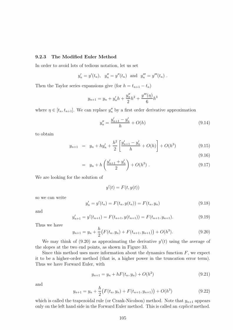
9.2.3 The Modified Euler Method
In order to avoid lots of tedious notation, let us set
y′n = y′(tn), y′′
n = y′′(tn) and y′′′n = y′′′(tn) .
Then the Taylor series expansions give (for h = tn+1 − tn)
yn+1 = yn + y′nh +
y′′n
2h2 +
y′′′(η)
6h3
where η ∈ [tn, tn+1]. We can replace y′′n by a first order derivative approximation
y′′n =
y′n+1 − y′
n
h+ O(h) (9.14)
to obtain
yn+1 = yn + hy′n +
h2
2
[
y′n+1 − y′
n
h+ O(h)
]
+ O(h3) (9.15)
(9.16)
= yn + h
(
y′n+1 + y′
n
2
)
+ O(h3) . (9.17)
We are looking for the solution of
y′(t) = F (t, y(t))
so we can writey′
n = y′(tn) = F (tn, y(tn)) = F (tn, yn) (9.18)
andy′
n+1 = y′(tn+1) = F (tn+1, y(tn+1)) = F (tn+1, yn+1). (9.19)
Thus we have
yn+1 = yn +h
2
(
F (tn, yn) + F (tn+1, yn+1))
+ O(h3). (9.20)
We may think of (9.20) as approximating the derivative y′(t) using the average ofthe slopes at the two end points, as shown in Figure 33.
Since this method uses more information about the dynamics function F , we expectit to be a higher-order method (that is, a higher power in the truncation error term).Thus we have Forward Euler, with
yn+1 = yn + hF (tn, yn) + O(h2) (9.21)
and
yn+1 = yn +h
2
(
F (tn, yn) + F (tn+1, yn+1))
+ O(h3) (9.22)
which is called the trapezoidal rule (or Crank-Nicolson) method. Note that yn+1 appearsonly on the left hand side in the Forward Euler method. This is called an explicit method.
105
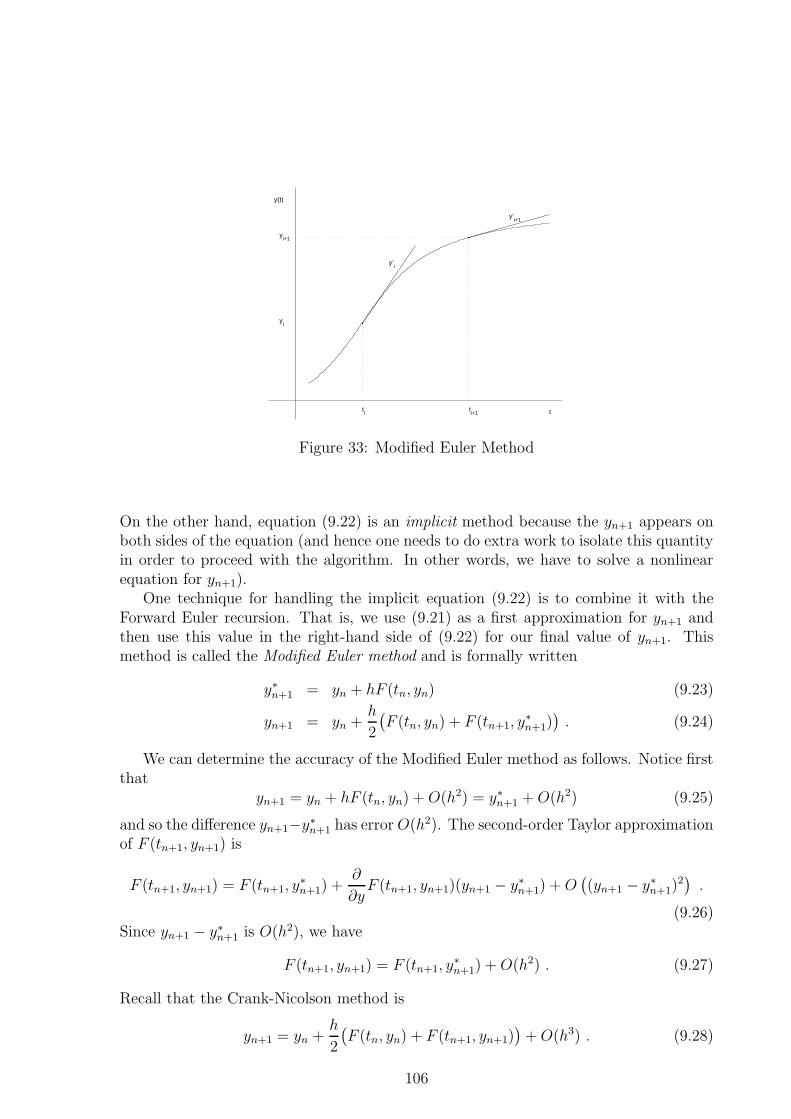
t
y(t)
ti
ti+1
yi
yi+1
y’i
y’i+1
Figure 33: Modified Euler Method
On the other hand, equation (9.22) is an implicit method because the yn+1 appears onboth sides of the equation (and hence one needs to do extra work to isolate this quantityin order to proceed with the algorithm. In other words, we have to solve a nonlinearequation for yn+1).
One technique for handling the implicit equation (9.22) is to combine it with theForward Euler recursion. That is, we use (9.21) as a first approximation for yn+1 andthen use this value in the right-hand side of (9.22) for our final value of yn+1. Thismethod is called the Modified Euler method and is formally written
y∗n+1 = yn + hF (tn, yn) (9.23)
yn+1 = yn +h
2
(
F (tn, yn) + F (tn+1, y∗n+1)
)
. (9.24)
We can determine the accuracy of the Modified Euler method as follows. Notice firstthat
yn+1 = yn + hF (tn, yn) + O(h2) = y∗n+1 + O(h2) (9.25)
and so the difference yn+1−y∗n+1 has error O(h2). The second-order Taylor approximation
of F (tn+1, yn+1) is
F (tn+1, yn+1) = F (tn+1, y∗n+1) +
∂
∂yF (tn+1, yn+1)(yn+1 − y∗
n+1) + O(
(yn+1 − y∗n+1)
2)
.
(9.26)Since yn+1 − y∗
n+1 is O(h2), we have
F (tn+1, yn+1) = F (tn+1, y∗n+1) + O(h2) . (9.27)
Recall that the Crank-Nicolson method is
yn+1 = yn +h
2
(
F (tn, yn) + F (tn+1, yn+1))
+ O(h3) . (9.28)
106
Therefore, plugging (9.27) into (9.28) gives
yn+1 = yn +h
2
(
F (tn, yn) + F (tn+1, y∗n+1) + O(h2)
)
+ O(h3) (9.29)
= yn +h
2
(
F (tn, yn) + F (tn+1, y∗n+1)
)
+ O(h3) . (9.30)
Thus we have that
y∗n+1 = yn + hF (tn, yn) (9.31)
yn+1 = yn +h
2(F (tn, yn) + F (tn+1, y
∗n+1)) + O(h3) (9.32)
is an explicit method with a higher-order truncation error than the Forward Eulermethod. We can also write this as
k1 = hF (tn, yn)
k2 = hF (tn + h, yn + k1)
yn+1 = yn + k1+k2
2.
This is an example of a Runge-Kutta method. There are many other possibilities forderiving explicit Runge-Kutta methods which have local error O(h3) due to truncation.For example, we have the midpoint Runge-Kutta method given by
k1 = hF (tn, yn)
k2 = hF (tn + h2, yn + k1
2)
yn+1 = yn + k2 .
which is also of order O(h3). One can continue on with such ideas in order to obtainmethods which have local truncation error O(hα) for α = 4, 5, 6, . . . The best knownexample of a higher order Runge-Kutta method is
k1 = hF (tn, yn)
k2 = hF (tn + h2, yn + k1
2)
k3 = hF (tn + h2, yn + k2
2)
k4 = hF (tn + h, yn + k3)
yn+1 = yn + k1
6+ k2
3+ k3
3+ k4
6,
a method having local error O(h5).
107
9.3 Global vs. Local Error
In the preceding subsection, we considered just the local truncation error for the ForwardEuler and Modified Euler methods. This is a local error in the sense that it is the errorwhen making a single step. In this section, we ask how this affects the global error afterwe make a large number of steps. For example, we are interested in y(tn)− yn for somefinite tn > t0.
If we consider, for example, the error when using Modified Euler, then we see thatwe have an error term O(h3) at each step. But these errors will accumulate from stepto step so that the global error in the computed solution at the last step will be larger(possibly by a significant amount) than the local error. In the worst case, all the localerrors accumulate. If we solve the differential equation to some time tn > t0, and if thestep size h is constant for all time steps, then
# steps =tn − t0
h= O
(
1
h
)
.
Therefore we haveGlobal Error ≤ Local Error ·# steps
= O(h3) ·O( 1h)
= O(h2).
In general, tn − t0 =∑n
k=1 hk with an average step-size of (tn − t0)/n with the globalerror being approximately equal to the sum of all the local errors.
One can see that if we have a method with local error O(hp+1) then the global erroris O(hp). In general, when we refer to the order of a method then we refer to the globalerror. Thus we say that Modified Euler is a second order method while Forward Euleris a first order method.
9.4 Practical Issues
The goal of ODE solvers is that for a specific tolerance we determine a set of points tnand yn such that the local error at the nth step is less than this tolerance. In previoussections we have focussed on the approximation step, that is, the step to determine theyn. For any particular problem, this part requires only knowledge of F (t, y(t)). Forexample, one has Modified Euler which can be given as a Runge-Kutta method:
k1 = hF (tn, yn)k2 = hF (tn + h, yn + k1)
yn+1 = yn + k1+k2
2.
Software Libraries can be developed for the various methods so that the user is onlyrequired to supply a function which evaluates F (t, y) for any (t, y). This is the approachused by Matlab ODE suite, for example. The cost and efficiency of any method can bemeasured by the number of function evaluations required – that is, the number of times
108
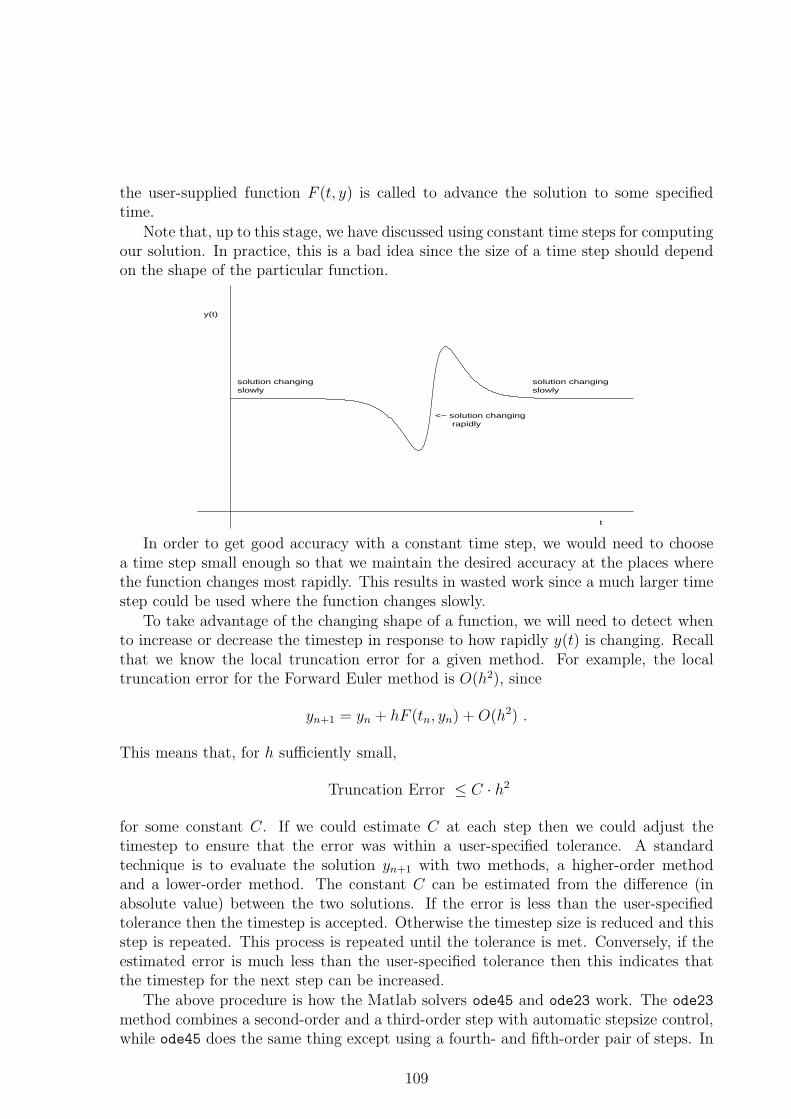
the user-supplied function F (t, y) is called to advance the solution to some specifiedtime.
Note that, up to this stage, we have discussed using constant time steps for computingour solution. In practice, this is a bad idea since the size of a time step should dependon the shape of the particular function.
solution changingslowly
<− solution changing rapidly
solution changingslowly
t
y(t)
In order to get good accuracy with a constant time step, we would need to choosea time step small enough so that we maintain the desired accuracy at the places wherethe function changes most rapidly. This results in wasted work since a much larger timestep could be used where the function changes slowly.
To take advantage of the changing shape of a function, we will need to detect whento increase or decrease the timestep in response to how rapidly y(t) is changing. Recallthat we know the local truncation error for a given method. For example, the localtruncation error for the Forward Euler method is O(h2), since
yn+1 = yn + hF (tn, yn) + O(h2) .
This means that, for h sufficiently small,
Truncation Error ≤ C · h2
for some constant C. If we could estimate C at each step then we could adjust thetimestep to ensure that the error was within a user-specified tolerance. A standardtechnique is to evaluate the solution yn+1 with two methods, a higher-order methodand a lower-order method. The constant C can be estimated from the difference (inabsolute value) between the two solutions. If the error is less than the user-specifiedtolerance then the timestep is accepted. Otherwise the timestep size is reduced and thisstep is repeated. This process is repeated until the tolerance is met. Conversely, if theestimated error is much less than the user-specified tolerance then this indicates thatthe timestep for the next step can be increased.
The above procedure is how the Matlab solvers ode45 and ode23 work. The ode23
method combines a second-order and a third-order step with automatic stepsize control,while ode45 does the same thing except using a fourth- and fifth-order pair of steps. In
109
both cases, the user supplies a tolerance. The estimates are not perfect of course, butin practice the methods work very well.
As an example, the formulas for the ode45 method (known as the Runge-Kutta-Fehlberg formula) is given by
k1 = hF (tn, yn)
k2 = hF (tn + h4, yn + k1
4)
k3 = hF (tn + 3h8, yn + 3k1
32+ 9k2
32)
k4 = hF (tn + 12h13
, yn + 1932k1
2197− 7200k2
2197+ 7296k3
2197)
k5 = hF (tn + h, yn + 439k1
216− 8k2 + 3680k3
513− 845k4
4104)
k6 = hF (tn + h2, yn − 8k1
27+ 2k2 − 3544k3
2565+ 1859k4
4104− 11k5
40)
y∗n+1 = yn + 25k1
216+ 1408k3
2565+ 2197k4
4104− k5
5with error O(h4)
yn+1 = yn + 16k1
135+ 6656k3
12825+ 28561k4
56430− 9k5
50+ 2k6
55with error O(h5) .
In this case the error can be estimated by
Error = yn+1 − y∗n+1 =
k1
360− 128k3
4275− 2197k4
75240+
k5
50+
2k6
55.
9.5 Overview of Numerical Methods and the Matlab ODE Suite
In §9.2, we introduced the idea of a numerical solution of an IVP and discussed methodsfor computing them. We noted that a numerical method has the coupled pair of tasks:
advancing the solution: computing y(n) - which we now designate with a bracketedsuperscript since it is an m vector, y(n) = (y
(n)1 , y
(n)2 , . . . y
(n)m )
time step size selection: computing tn
We repeat the conceptual scheme for time stepping methods here.
Initialize y(0), t0, hcand, n = 0
Repeat
i) compute y(n+1), and hn using data tn, y(n), hcand and f(t, z)
ii) tn+1 ← tn + hn
iii) recompute hcand
iv) n← n + 1
(9.33)
110
9.5.1 Classification of methods for advancing the solution
The exact solution of a system of ODEs (8.9) satisfies
y(tn+1) = y(tn) +
∫ tn+1
tn
y′(s)ds = y(tn) + M−1
∫ tn+1
tn
f(s, y(s))ds
= y(tn) + hnM−1Avg(f) (9.34)
where Avg(f) is an average value of the dynamics function over the trajectory in theinterval tn < s < tn+1 which is of length hn, i.e.
Avg(f) =1
hn
∫ tn+1
tn
f(s, y(s))ds (9.35)
If M 6= I, then to implement (9.34), a system of linear equations, Mx = Avg(f), wouldhave to be solved for x and then y(tn+1) could be computed as
y(tn+1) = y(tn) + hnx .
Of course, even if we know tn, tn+1 and y(tn), the relation in (9.34) cannot be used tocompute y(tn+1) exactly because we cannot evaluate the integral term. Actually, thereare two difficulties associated with this integral term.
i) We do not know y(s), hence we do not know the integrand function.
ii) Even if we did, we would not usually be able to integrate it by an explicit formula.
Most time stepping methods for advancing the solution can be viewed as approximateevaluations of this integral, or, equivalently, this average. The simplest example is theapproximation
Avg(f) ≈ f(tn, y(tn)) (9.36)
which is equivalent to the Forward Euler’s method.There are several standard general classifications of solution computation methods.
One is the classification into:
One-step methods in which (tn+1, y(n+1)) is computed from (tn, y(n)), (using f(t, z)
and M).
Multi-step methods in which (tn+1, y(n+1)) is computed from (tn−k, y
(n−k)) for k =0, 1, . . . , Nsteps, where Nsteps > 0.
Another standard classification is into:
Explicit methods in which y(n+1) is computed by a formula involving tn−j and y(n−j)
and evaluations of f(t, z), j = 0, 1, ...Nsteps, where Nsteps ≥ 0.
Implicit methods in which y(n+1) is computed by solving an algebraic system of equa-tions that involve f(t, z).
111
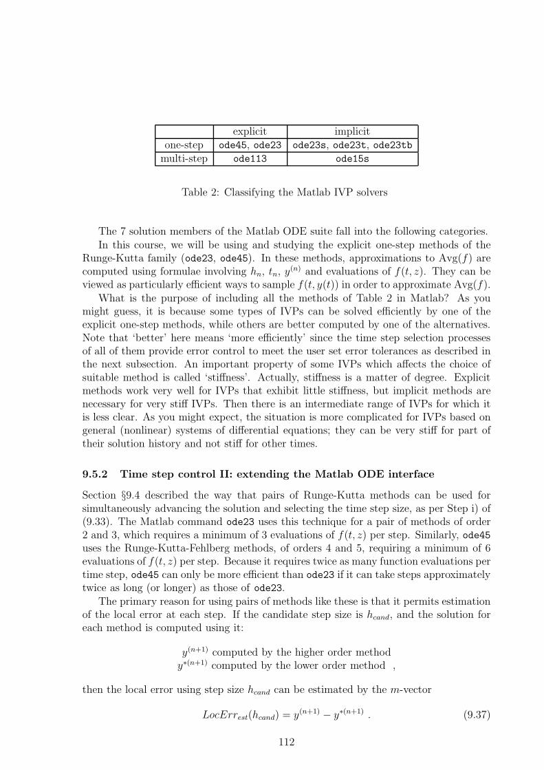
explicit implicitone-step ode45, ode23 ode23s, ode23t, ode23tb
multi-step ode113 ode15s
Table 2: Classifying the Matlab IVP solvers
The 7 solution members of the Matlab ODE suite fall into the following categories.In this course, we will be using and studying the explicit one-step methods of the
Runge-Kutta family (ode23, ode45). In these methods, approximations to Avg(f) arecomputed using formulae involving hn, tn, y(n) and evaluations of f(t, z). They can beviewed as particularly efficient ways to sample f(t, y(t)) in order to approximate Avg(f).
What is the purpose of including all the methods of Table 2 in Matlab? As youmight guess, it is because some types of IVPs can be solved efficiently by one of theexplicit one-step methods, while others are better computed by one of the alternatives.Note that ‘better’ here means ‘more efficiently’ since the time step selection processesof all of them provide error control to meet the user set error tolerances as described inthe next subsection. An important property of some IVPs which affects the choice ofsuitable method is called ‘stiffness’. Actually, stiffness is a matter of degree. Explicitmethods work very well for IVPs that exhibit little stiffness, but implicit methods arenecessary for very stiff IVPs. Then there is an intermediate range of IVPs for which itis less clear. As you might expect, the situation is more complicated for IVPs based ongeneral (nonlinear) systems of differential equations; they can be very stiff for part oftheir solution history and not stiff for other times.
9.5.2 Time step control II: extending the Matlab ODE interface
Section §9.4 described the way that pairs of Runge-Kutta methods can be used forsimultaneously advancing the solution and selecting the time step size, as per Step i) of(9.33). The Matlab command ode23 uses this technique for a pair of methods of order2 and 3, which requires a minimum of 3 evaluations of f(t, z) per step. Similarly, ode45uses the Runge-Kutta-Fehlberg methods, of orders 4 and 5, requiring a minimum of 6evaluations of f(t, z) per step. Because it requires twice as many function evaluations pertime step, ode45 can only be more efficient than ode23 if it can take steps approximatelytwice as long (or longer) as those of ode23.
The primary reason for using pairs of methods like these is that it permits estimationof the local error at each step. If the candidate step size is hcand, and the solution foreach method is computed using it:
y(n+1) computed by the higher order methody∗(n+1) computed by the lower order method ,
then the local error using step size hcand can be estimated by the m-vector
LocErrest(hcand) = y(n+1) − y∗(n+1) . (9.37)
112
The step size is chosen to ensure that the size of LocErrest is less than a specified errortolerance. The basic concept is that
if maxk |LocErrest(hcand)k| ≤ tol thenaccept hcand as hn
elsereduce hcand and try again
end if
The Matlab ODE suite has three options for customizing this concept for error control,associated with properties named AbsTol, RelTol, and NormControl. See §8.5.2 for adiscussion of ‘properties’ and options. Here are descriptions of these properties from“help odeset”.
RelTol - Relative error tolerance [ positive scalar {1e-3} ]
This scalar applies to all components of the solution vector, and
defaults to 1e-3 (0.1% accuracy) in all solvers. The estimated error in
each integration step satisfies e(i) <= max(RelTol*abs(y(i)),AbsTol(i)).
AbsTol - Absolute error tolerance [ positive scalar or vector {1e-6} ]
A scalar tolerance applies to all components of the solution vector.
Elements of a vector of tolerances apply to corresponding components of
the solution vector. AbsTol defaults to 1e-6 in all solvers. See RelTol.
NormControl - Control error relative to norm of solution [ on | {off} ]
Set this property ’on’ to request that the solvers control the error in
each integration step with norm(e) <= max(RelTol*norm(y),AbsTol). By
default the solvers use a more stringent component-wise error control.
Matlab also has several properties that control the form of the output from callingodeX. Two of these that are of interest to us are named
Refine which takes positive integer values and determines the number of output timesper time step
Stats which take binary values, i.e.’on’ or ’off. This property determines whether odeXdisplays a summary of cost statistics for the computation
In these notes, we have use hn = tn+1 − tn as the step size, and implied that theoutput vector, T(n), of Matlab’s odeX functions is composed of exactly these time valuestn. So the entire stepsize history would be the vector
h = T(2:length(T)) - T(1:length(T)-1) . (9.38)
However, this is only true if Refine = 1. The default value for Refine is 1 for allmethods except ode45, where its default value is 4. To compute the stepsize history forode45 using (9.38), you must use the function odeset to set Refine = 1 (see §8.5.2).
113
Exercises
1. Suppose a function y(t) is known at three discrete points ti, ti−1, ti−2, whereti − ti−1 6= ti−1 − ti−2. Use Taylor series arguments to determine a backwarddifference approximation to y′′
i , using three values yi, yi−1, yi−2. What is your ordercondition?
2. Verify for the following system of equations
Y ′1 = Y2
Y ′2 = −x2Y1 − xY2
that Y1(x) = y(x), where y(x) satisfies the second order equation
y′′(x) + x y′(x) + x2 y(x) = 0 .
3. Write the following third order differential equation as a system of three first-orderequations.
y′′′(t) + sin(t)y′′(t)− g(t)y′(t) + g(t)y(t) = f(t)
4. State the following problem in first order form. Differentiation is with respect tot.
u′′ + 3v′ + 4u + v = tu′′ − v′ + u + v = cos t
5. Apply both the Forward Euler and the Modified Euler methods to the IVP
{
y′ = 5yy(0) = 5 .
Show the computation schemes for both methods
6. Suppose you are using an ODE solver to compute an approximate solution tothe equation y′ = F (t, y). At some point ti you have an approximate solution yi.
Using the solver, you compute estimates yhi+1 and y
h/2i+1 using steps h and h/2, where
h = 0.01. Note that the second estimate involves applying the ODE solver twice,first to get to ti+ 1
2, and then again to get from ti+ 1
2to ti+1. The method you are
using is a second order method with third order local truncation error. Supposeyh
i+1 = 3.269472 · · · and yh/2i+1 = 3.269374 · · · . That is, ‖yh
i+1 − yh/2i+1‖ ≈ 10−4.
Derive an estimate for the local truncation error at the point ti+1. Show carefullyhow you arrived at your estimate.
114
Appendix A Conveying Information in Graphs
Figures and graphics can be a powerful way to communicate ideas; they play a keyrole for this purpose in scientific computation. However, the use of graphics to enhancecommunication requires effort and skill. And while a good graphics package helps, itis really only a tool. Many other factors play into the successful use of graphics toconvey a message (just as a hammer is a useful tool, but one needs expertise to build ahouse). Lets make a comparison with the task of writing a document using text aloneto help explain what is meant by this. Obviously, word processors are a very usefultool for supporting this task. But the effectiveness of the communication comes fromthe combination of the writer’s ability to express themselves and how they use the tool.The writer needs clarity about what is to be conveyed and how to organize it into prose.The word processor doesn’t help with this. But creating an effective document canalso be strongly enhanced by an understanding of the variety of options that a wordprocessor can offer for the task. Success comes from the combination of author’s effort,word processor functionality, author’s skill with it and the author’s patience, time, andenergy.
The same is true of conveying ideas graphically; graphics systems (MATLAB graphicsincluded) are indispensable tools for the task. But to use them successfully, one needs
• skill in creating meaningful images,
• understanding of the capabilities of the tool, and
• patience, time, and energy.
In this section, we hope to introduce some of the basics of how MATLAB graphics can beused to convey ideas effectively by an example based on parametric curve computations.
Figure 34 shows four subplots generated by the MATLAB ‘subplot(2,2,X)’ command.See the script at the end of this appendix. The plot in the X=1 position (the upperleft corner) shows the curve created using piecewise linear interpolation of the data,generated using a single MATLAB “plot” command (and, consequently, all the defaultimage settings for this command). It is not clear what message this plot might beintended to convey; the default plot settings are simply designed to allow a user toquickly and easily display a wide spectrum of data on a screen. Some of the weaknessesof that particular plot for displaying the script letter are:
• The axes are scaled differently, so the figure is distorted.
• The tic mark labelling on the axes would be too small to be readable if the imageis shrunk for printing.
• There is no text (no axis variable labelling, no title line) to guide the reader.
This crude picture would need to be accompanied by a lot of text to explain what itsmessage is. The other three subplots show figures customized to convey three specificideas:
115
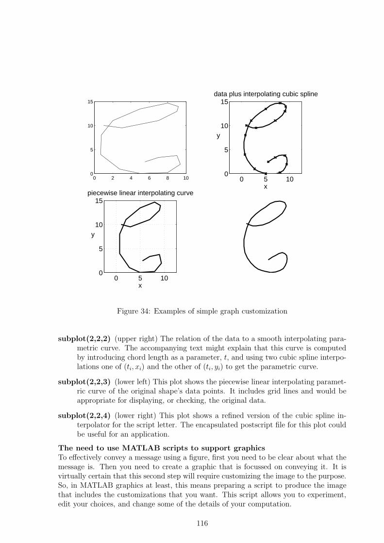
0 2 4 6 8 100
5
10
15
0 5 100
5
10
15data plus interpolating cubic spline
x
y
0 5 100
5
10
15piecewise linear interpolating curve
x
y
Figure 34: Examples of simple graph customization
subplot(2,2,2) (upper right) The relation of the data to a smooth interpolating para-metric curve. The accompanying text might explain that this curve is computedby introducing chord length as a parameter, t, and using two cubic spline interpo-lations one of (ti, xi) and the other of (ti, yi) to get the parametric curve.
subplot(2,2,3) (lower left) This plot shows the piecewise linear interpolating paramet-ric curve of the original shape’s data points. It includes grid lines and would beappropriate for displaying, or checking, the original data.
subplot(2,2,4) (lower right) This plot shows a refined version of the cubic spline in-terpolator for the script letter. The encapsulated postscript file for this plot couldbe useful for an application.
The need to use MATLAB scripts to support graphicsTo effectively convey a message using a figure, first you need to be clear about what themessage is. Then you need to create a graphic that is focussed on conveying it. It isvirtually certain that this second step will require customizing the image to the purpose.So, in MATLAB graphics at least, this means preparing a script to produce the imagethat includes the customizations that you want. This script allows you to experiment,edit your choices, and change some of the details of your computation.
116
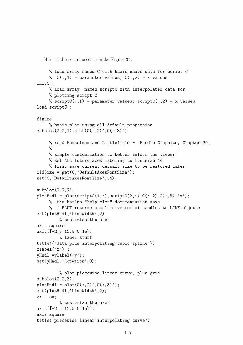
Here is the script used to make Figure 34:
% load array named C with basic shape data for script C
% C(:,1) = parameter values; C(:,2) = x values
initC ;
% load array named scriptC with interpolated data for
% plotting script C
% scriptC(:,1) = parameter values; scriptC(:,2) = x values
load scriptC ;
figure
% basic plot using all default properties
subplot(2,2,1),plot(C(:,2)’,C(:,3)’)
% read Hanselman and Littlefield - Handle Graphics, Chapter 30,
%
% simple customization to better inform the viewer
% set ALL future axes labeling to fontsize 14
% first save current defualt size to be restored later
oldSize = get(0,’DefaultAxesFontSize’);
set(0,’DefaultAxesFontSize’,14);
subplot(2,2,2),
plotHndl = plot(scriptC(1,:),scriptC(2,:),C(:,2),C(:,3),’x’);
% the Matlab "help plot" documentation says
% ’ PLOT returns a column vector of handles to LINE objects
set(plotHndl,’LineWidth’,2)
% customize the axes
axis square
axis([-2.5 12.5 0 15])
% label stuff
title({’data plus interpolating cubic spline’})
xlabel(’x’) ;
yHndl =ylabel(’y’);
set(yHndl,’Rotation’,0);
% plot piecewise linear curve, plus grid
subplot(2,2,3),
plotHndl = plot(C(:,2)’,C(:,3)’);
set(plotHndl,’LineWidth’,2);
grid on;
% customize the axes
axis([-2.5 12.5 0 15]);
axis square
title(’piecewise linear interpolating curve’)
117
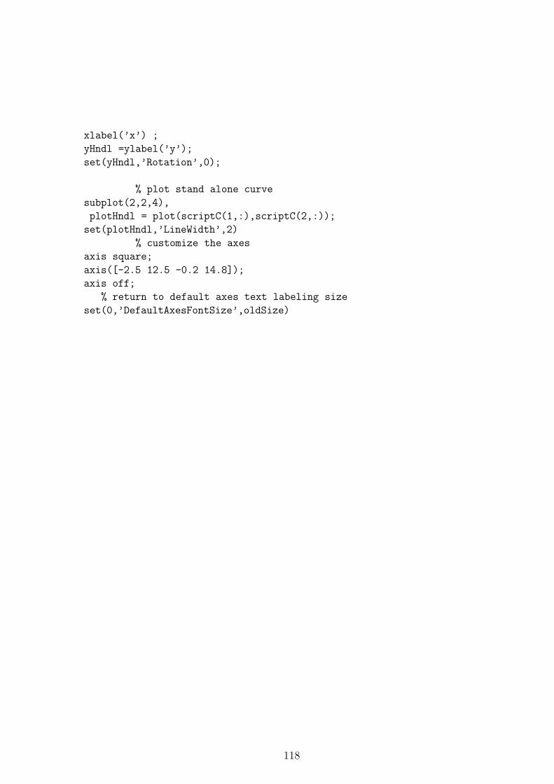
xlabel(’x’) ;
yHndl =ylabel(’y’);
set(yHndl,’Rotation’,0);
% plot stand alone curve
subplot(2,2,4),
plotHndl = plot(scriptC(1,:),scriptC(2,:));
set(plotHndl,’LineWidth’,2)
% customize the axes
axis square;
axis([-2.5 12.5 -0.2 14.8]);
axis off;
% return to default axes text labeling size
set(0,’DefaultAxesFontSize’,oldSize)
118
Appendix B Review of Complex Numbers
We will denote the set of complex numbers by C. A complex number z ∈ C can beidentified as a pair of real numbers; i.e. z = (a, b). A standard (historical) notation forz involves the symbol i which may be called “the square root of -1” and identified with√−1. In this notation z is written z = a + ib and
• i can be identified with (0, 1).
• a is called the real part of z; a = Real(z).
• b is called the imaginary part of z: b = Imag(z).
• In Matlab, the command display( complex(-3,2) ) will display-3.000 + 2.000 i.
• a− ib is called the conjugate of z, sometimes denoted by z.
• The size of z is |z| =√
a2 + b2, also called the modulus of z.
Arithmetic operations are defined for C: let z = (a, b) and r = (c, d) ∈ C
• z + r = (a + c, b + d),
• z × r = (ac− bd, ad + cb). Usually we will just write zr for z × r.
A real number, x, is the same as the complex number (x, 0). Notice that if z = (x, 0)and r = (y, 0), then the addition and multiplication of z and r are the same as addingand multiplying in the real number system. In this sense, the complex number systemis “backwards compatible”, so to speak. Thus, we do not need to make any furtherdistinction between x and (x, 0). You will find that Matlab does not distinguish betweenthese either; try y = complex(2,0) in Matlab. Some other interesting relations fromthe above definitions are z + z = 2 Real(z), and zz = |z|2 = a2 + b2.
We can form a vector of N complex numbers, u = (u1, u2, . . . , uN)t, and
• multiply u by a number p ∈ C.
• add two complex vectors together. In fact, we can make linear combinations ofthem. i.e. for two complex vectors u and v (of the same size and shape) and twocomplex numbers e and f , eu + fv is also a complex vector.
• take the inner product of two complex vectors u and v using
(u, v) =
N∑
j=1
uj vj . (B.1)
119
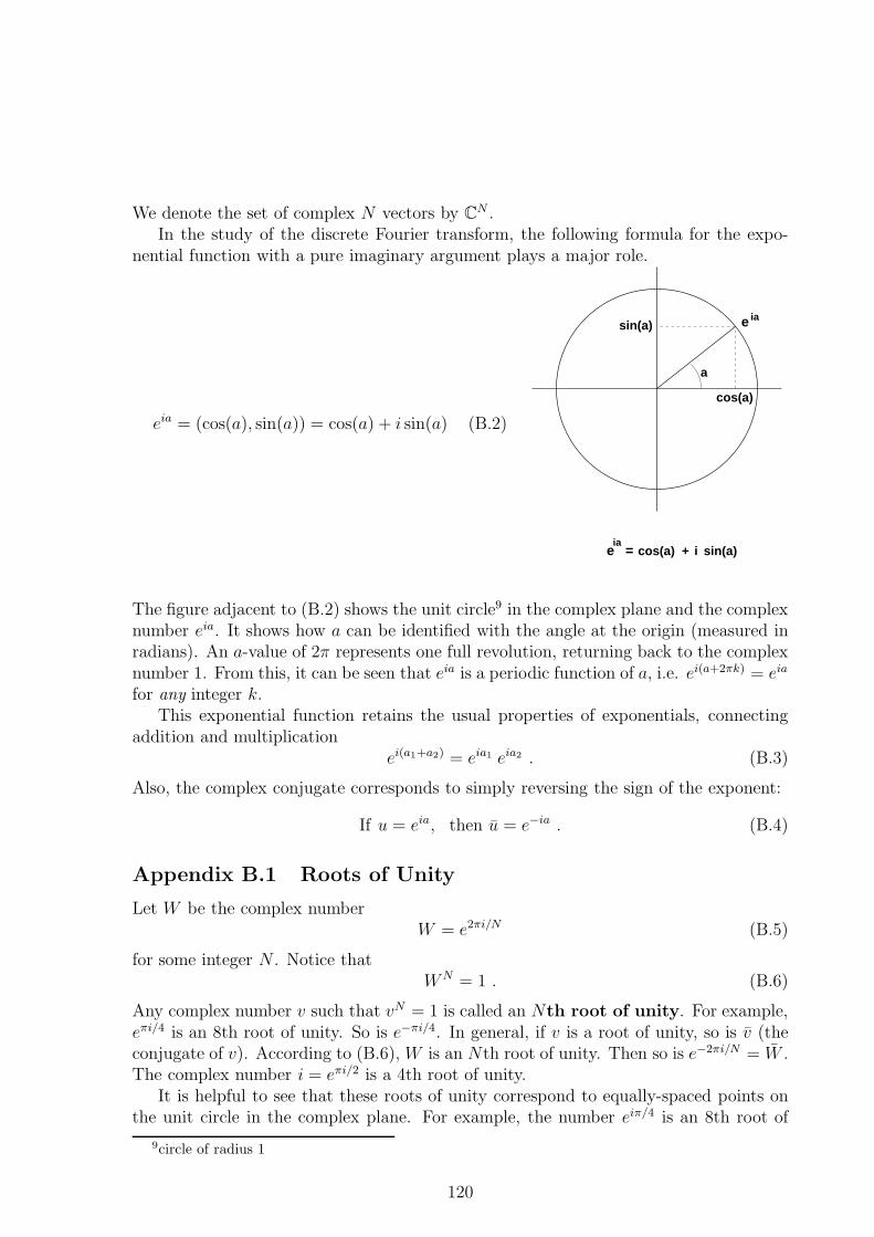
We denote the set of complex N vectors by CN .In the study of the discrete Fourier transform, the following formula for the expo-
nential function with a pure imaginary argument plays a major role.
eia = (cos(a), sin(a)) = cos(a) + i sin(a) (B.2)
esin(a)
cos(a)
a
ia
eia
= sin(a)cos(a) + i
The figure adjacent to (B.2) shows the unit circle9 in the complex plane and the complexnumber eia. It shows how a can be identified with the angle at the origin (measured inradians). An a-value of 2π represents one full revolution, returning back to the complexnumber 1. From this, it can be seen that eia is a periodic function of a, i.e. ei(a+2πk) = eia
for any integer k.This exponential function retains the usual properties of exponentials, connecting
addition and multiplicationei(a1+a2) = eia1 eia2 . (B.3)
Also, the complex conjugate corresponds to simply reversing the sign of the exponent:
If u = eia, then u = e−ia . (B.4)
Appendix B.1 Roots of Unity
Let W be the complex numberW = e2πi/N (B.5)
for some integer N . Notice thatW N = 1 . (B.6)
Any complex number v such that vN = 1 is called an Nth root of unity. For example,eπi/4 is an 8th root of unity. So is e−πi/4. In general, if v is a root of unity, so is v (theconjugate of v). According to (B.6), W is an Nth root of unity. Then so is e−2πi/N = W .The complex number i = eπi/2 is a 4th root of unity.
It is helpful to see that these roots of unity correspond to equally-spaced points onthe unit circle in the complex plane. For example, the number eiπ/4 is an 8th root of
9circle of radius 1
120
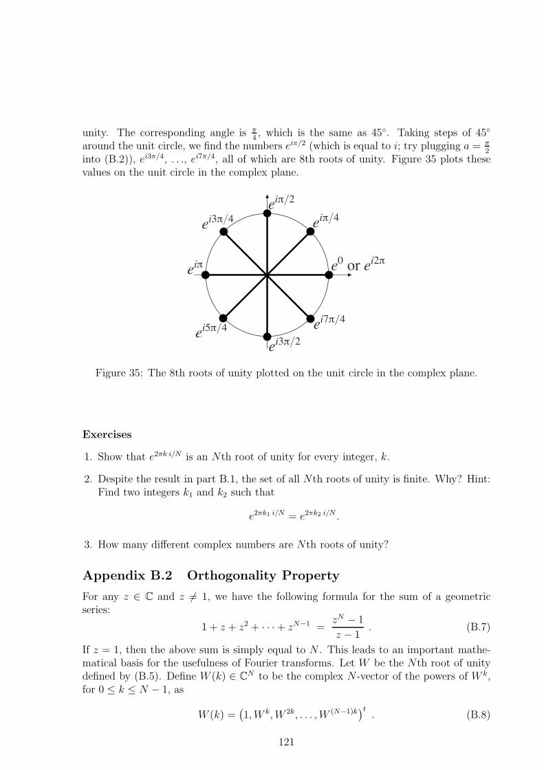
unity. The corresponding angle is π4, which is the same as 45◦. Taking steps of 45◦
around the unit circle, we find the numbers eiπ/2 (which is equal to i; try plugging a = π2
into (B.2)), ei3π/4, . . ., ei7π/4, all of which are 8th roots of unity. Figure 35 plots thesevalues on the unit circle in the complex plane.
e0or e
i2π
ei7π/4
ei5π/4
ei3π/2
ei3π/4
eiπ/2
eiπ
eiπ/4
Figure 35: The 8th roots of unity plotted on the unit circle in the complex plane.
Exercises
1. Show that e2πk i/N is an Nth root of unity for every integer, k.
2. Despite the result in part B.1, the set of all Nth roots of unity is finite. Why? Hint:Find two integers k1 and k2 such that
e2πk1 i/N = e2πk2 i/N .
3. How many different complex numbers are Nth roots of unity?
Appendix B.2 Orthogonality Property
For any z ∈ C and z 6= 1, we have the following formula for the sum of a geometricseries:
1 + z + z2 + · · ·+ zN−1 =zN − 1
z − 1. (B.7)
If z = 1, then the above sum is simply equal to N . This leads to an important mathe-matical basis for the usefulness of Fourier transforms. Let W be the Nth root of unitydefined by (B.5). Define W (k) ∈ CN to be the complex N -vector of the powers of W k,for 0 ≤ k ≤ N − 1, as
W (k) =(
1, W k, W 2k, . . . , W (N−1)k)t
. (B.8)
121
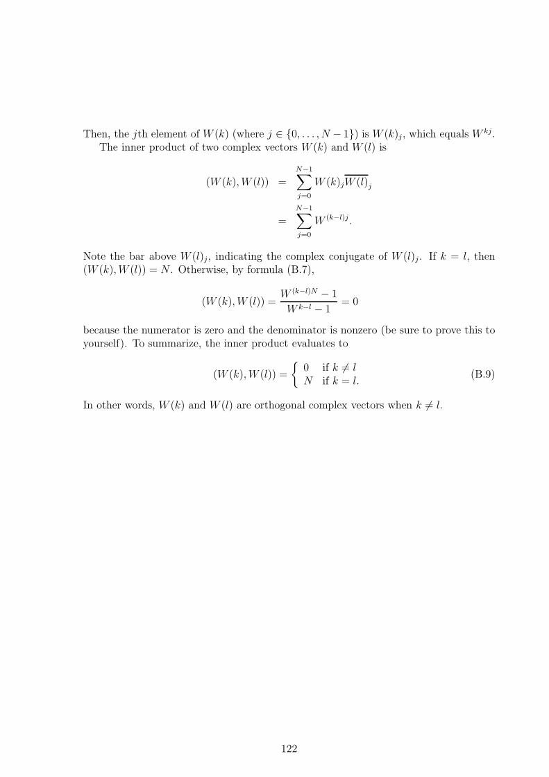
Then, the jth element of W (k) (where j ∈ {0, . . . , N − 1}) is W (k)j, which equals W kj.The inner product of two complex vectors W (k) and W (l) is
(W (k), W (l)) =
N−1∑
j=0
W (k)jW (l)j
=N−1∑
j=0
W (k−l)j.
Note the bar above W (l)j, indicating the complex conjugate of W (l)j. If k = l, then(W (k), W (l)) = N . Otherwise, by formula (B.7),
(W (k), W (l)) =W (k−l)N − 1
W k−l − 1= 0
because the numerator is zero and the denominator is nonzero (be sure to prove this toyourself). To summarize, the inner product evaluates to
(W (k), W (l)) =
{
0 if k 6= lN if k = l.
(B.9)
In other words, W (k) and W (l) are orthogonal complex vectors when k 6= l.
122