lecture notes on parallel scientiﬁc computingtyang/class/110b02/notes02.pdf · lecture notes on...

Lecture Notes on Parallel Scientific ComputingTao Yang ([email protected])

Contents

1 Introduction 3

2 Design and Implementation of Parallel Algorithms 5

2.1 A simple model of parallel computation . . . . . . . . . . . . . . . . . . . . . . . . . . . . . . . . . . . 5

2.2 Message-Passing Parallel Programming . . . . . . . . . . . . . . . . . . . . . . . . . . . . . . . . . . . . 6

2.3 Complexity analysis for parallel algorithms . . . . . . . . . . . . . . . . . . . . . . . . . . . . . . . . . 8

3 Model-based Programming Methods 10

3.1 Embarrassingly Parallel Computations . . . . . . . . . . . . . . . . . . . . . . . . . . . . . . . . . . . . 10

3.1.1 Geometrical Transformations of Images . . . . . . . . . . . . . . . . . . . . . . . . . . . . . . . 10

3.1.2 Mandelbrot Set . . . . . . . . . . . . . . . . . . . . . . . . . . . . . . . . . . . . . . . . . . . . . 11

3.1.3 Monte Carlo Methods . . . . . . . . . . . . . . . . . . . . . . . . . . . . . . . . . . . . . . . . . 12

3.2 Divide-and-Conquer . . . . . . . . . . . . . . . . . . . . . . . . . . . . . . . . . . . . . . . . . . . . . . 14

3.2.1 Add n numbers . . . . . . . . . . . . . . . . . . . . . . . . . . . . . . . . . . . . . . . . . . . . . 14

3.3 Pipelined Computations . . . . . . . . . . . . . . . . . . . . . . . . . . . . . . . . . . . . . . . . . . . . 15

3.3.1 Sorting n numbers . . . . . . . . . . . . . . . . . . . . . . . . . . . . . . . . . . . . . . . . . . . 15

4 Transformation-based Parallel Programming 16

4.1 Dependence Analysis . . . . . . . . . . . . . . . . . . . . . . . . . . . . . . . . . . . . . . . . . . . . . . 16

4.1.1 Basic dependence . . . . . . . . . . . . . . . . . . . . . . . . . . . . . . . . . . . . . . . . . . . . 16

4.1.2 Loop Parallelism . . . . . . . . . . . . . . . . . . . . . . . . . . . . . . . . . . . . . . . . . . . . 17

4.2 Program Partitioning . . . . . . . . . . . . . . . . . . . . . . . . . . . . . . . . . . . . . . . . . . . . . . 17

4.2.1 Loop blocking/unrolling . . . . . . . . . . . . . . . . . . . . . . . . . . . . . . . . . . . . . . . . 18

4.2.2 Interior loop blocking . . . . . . . . . . . . . . . . . . . . . . . . . . . . . . . . . . . . . . . . . 18

4.2.3 Loop interchange . . . . . . . . . . . . . . . . . . . . . . . . . . . . . . . . . . . . . . . . . . . . 19

4.3 Data Partitioning . . . . . . . . . . . . . . . . . . . . . . . . . . . . . . . . . . . . . . . . . . . . . . . . 21

4.3.1 Data partitioning methods . . . . . . . . . . . . . . . . . . . . . . . . . . . . . . . . . . . . . . 21

4.3.2 Consistency between program and data partitioning . . . . . . . . . . . . . . . . . . . . . . . . 22

4.3.3 Data indexing between global space and local space . . . . . . . . . . . . . . . . . . . . . . . . 23

4.4 A summary on program parallelization . . . . . . . . . . . . . . . . . . . . . . . . . . . . . . . . . . . . 24

5 Matrix Vector Multiplication 25

6 Matrix-Matrix Multiplication 26

1

6.1 Sequential algorithm . . . . . . . . . . . . . . . . . . . . . . . . . . . . . . . . . . . . . . . . . . . . . . 26

6.2 Parallel algorithm with sufficient memory . . . . . . . . . . . . . . . . . . . . . . . . . . . . . . . . . . 27

6.3 Parallel algorithm with 1D partitioning . . . . . . . . . . . . . . . . . . . . . . . . . . . . . . . . . . . 28

6.4 Fox’s algorithm for 2D data partitioning . . . . . . . . . . . . . . . . . . . . . . . . . . . . . . . . . . . 29

6.4.1 Reorder the sequential additions. . . . . . . . . . . . . . . . . . . . . . . . . . . . . . . . . . . . 29

6.4.2 Submatrix partitioning for block-based matrix multiplication . . . . . . . . . . . . . . . . . . . 30

6.5 How to produce block-based matrix multiplication code . . . . . . . . . . . . . . . . . . . . . . . . . . 31

7 Gaussian Elimination for Solving Linear Systems 32

7.1 Gaussian Elimination without Partial Pivoting . . . . . . . . . . . . . . . . . . . . . . . . . . . . . . . 32

7.1.1 The Row-Oriented GE sequential algorithm . . . . . . . . . . . . . . . . . . . . . . . . . . . . . 32

7.1.2 The row-oriented parallel algorithm . . . . . . . . . . . . . . . . . . . . . . . . . . . . . . . . . 33

7.1.3 The column-oriented algorithm . . . . . . . . . . . . . . . . . . . . . . . . . . . . . . . . . . . . 35

8 Gaussian elimination with partial pivoting 37

8.1 The sequential algorithm . . . . . . . . . . . . . . . . . . . . . . . . . . . . . . . . . . . . . . . . . . . . 37

8.2 Parallel column-oriented GE with pivoting . . . . . . . . . . . . . . . . . . . . . . . . . . . . . . . . . . 39

9 Iterative Methods for Solving Ax = b 40

9.1 The iterative methods . . . . . . . . . . . . . . . . . . . . . . . . . . . . . . . . . . . . . . . . . . . . . 40

9.2 Norms and Convergence . . . . . . . . . . . . . . . . . . . . . . . . . . . . . . . . . . . . . . . . . . . . 40

9.2.1 Norms of vectors and matrices . . . . . . . . . . . . . . . . . . . . . . . . . . . . . . . . . . . . 40

9.2.2 Convergence of iterative methods . . . . . . . . . . . . . . . . . . . . . . . . . . . . . . . . . . . 41

9.3 Jacobi Method for Ax = b . . . . . . . . . . . . . . . . . . . . . . . . . . . . . . . . . . . . . . . . . . . 42

9.4 Parallel Jacobi Method . . . . . . . . . . . . . . . . . . . . . . . . . . . . . . . . . . . . . . . . . . . . . 42

9.5 Gauss-Seidel Method . . . . . . . . . . . . . . . . . . . . . . . . . . . . . . . . . . . . . . . . . . . . . . 43

9.6 More on convergence. . . . . . . . . . . . . . . . . . . . . . . . . . . . . . . . . . . . . . . . . . . . . . 44

9.7 The SOR method . . . . . . . . . . . . . . . . . . . . . . . . . . . . . . . . . . . . . . . . . . . . . . . . 45

10 Numerical Differentiation 45

10.1 Approximation of Derivatives . . . . . . . . . . . . . . . . . . . . . . . . . . . . . . . . . . . . . . . . . 45

10.2 Central difference for second-derivatives . . . . . . . . . . . . . . . . . . . . . . . . . . . . . . . . . . . 46

10.3 Example . . . . . . . . . . . . . . . . . . . . . . . . . . . . . . . . . . . . . . . . . . . . . . . . . . . . . 46

11 ODE and PDE 47

11.1 Finite Difference Method . . . . . . . . . . . . . . . . . . . . . . . . . . . . . . . . . . . . . . . . . . . 47

11.2 Gaussian Elimination for solving linear tridiagonal systems . . . . . . . . . . . . . . . . . . . . . . . . 49

11.3 PDE: Laplace’s Equation . . . . . . . . . . . . . . . . . . . . . . . . . . . . . . . . . . . . . . . . . . . 50

2

A MPI Parallel Programming 55

B Pthreads 63

B.1 Introduction . . . . . . . . . . . . . . . . . . . . . . . . . . . . . . . . . . . . . . . . . . . . . . . . . . 63

B.2 Thread creation and manipulation . . . . . . . . . . . . . . . . . . . . . . . . . . . . . . . . . . . . . . 63

B.3 The Synchronization Routines: Lock . . . . . . . . . . . . . . . . . . . . . . . . . . . . . . . . . . . . . 65

B.4 Condition Variables . . . . . . . . . . . . . . . . . . . . . . . . . . . . . . . . . . . . . . . . . . . . . . 69

1 Introduction

• Scientific computing uses computers to analyze and solve scientific and engineering problems based onmathematical models. Applications of scientific computing include computer graphics, image Process-ing, stock analysis, weather, prediction, seismic data processing, design simulation (airplanes/cars),computational medicine, astrophysics, and nuclear Engineering.

• Parallel/cluster Computing. Solve problems in parallel on multiple machines.

• Applications of parallel computing: Large-scale scientific simulation, Parallel data bases (creditcards), multi-media information servers.

• Topics covered in 110B

– Introduction to parallel architectures. Model of Parallel Computers. Interconnection Network.Task graph computation.

– Message-passing parallel programming.

– Model-based parallel programming. Embarrassingly parallel, divide-and-conquer, and pipelin-ing.

– Transformation-based parallel programming. Dependence analysis. Partitioning and mappingof program/data.

– Parallel algorithms for scientific computing.

– Parallel programming on shared memory machines.

• Computer architectures: sequential machines, vector machines, parallel machines.

• Parallel architectures:

– Control mechanism. SIMD type (single instruction stream multiple data stream, e.g. MasParMP-1, CM-2). MIMD (multiple instruction stream multiple data stream, Meiko CS-2, IntelParagon, Cray T3E SP/2).

– Address-Space Organization. Message passing architecture (Cray T3E, IBM SP2). vs. SharedAddress space Architecture (SGI Origin 2000, SUN Enterprise).

• Interconnection network: bus, ring, hypercube, mesh.

Networked computers as a parallel machine.

• Motivation: High performance workstations and PCs are readily available at low cost. The latestprocessors can be upgraded easily. Existing software can be used or modified.

3

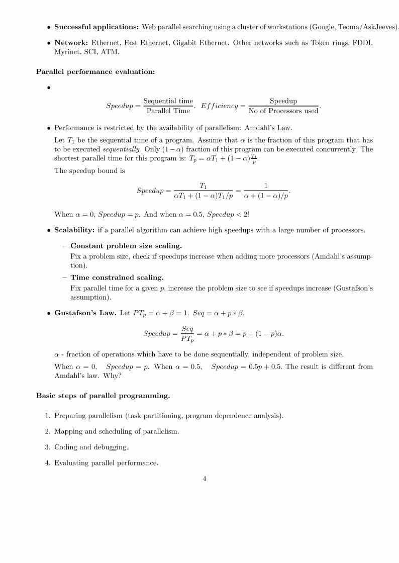
• Successful applications: Web parallel searching using a cluster of workstations (Google, Teoma/AskJeeves).

• Network: Ethernet, Fast Ethernet, Gigabit Ethernet. Other networks such as Token rings, FDDI,Myrinet, SCI, ATM.

Parallel performance evaluation:

•

Speedup =Sequential timeParallel Time

. Efficiency =Speedup

No of Processors used.

• Performance is restricted by the availability of parallelism: Amdahl’s Law.

Let T1 be the sequential time of a program. Assume that α is the fraction of this program that hasto be executed sequentially. Only (1−α) fraction of this program can be executed concurrently. Theshortest parallel time for this program is: Tp = αT1 + (1 − α)T1

p .

The speedup bound is

Speedup =T1

αT1 + (1 − α)T1/p=

1α + (1 − α)/p

.

When α = 0, Speedup = p. And when α = 0.5, Speedup < 2!

• Scalability: if a parallel algorithm can achieve high speedups with a large number of processors.

– Constant problem size scaling.Fix a problem size, check if speedups increase when adding more processors (Amdahl’s assump-tion).

– Time constrained scaling.Fix parallel time for a given p, increase the problem size to see if speedups increase (Gustafson’sassumption).

• Gustafson’s Law. Let PTp = α + β = 1. Seq = α + p ∗ β.

Speedup =Seq

PTp= α + p ∗ β = p + (1 − p)α.

α - fraction of operations which have to be done sequentially, independent of problem size.

When α = 0, Speedup = p. When α = 0.5, Speedup = 0.5p + 0.5. The result is different fromAmdahl’s law. Why?

Basic steps of parallel programming.

1. Preparing parallelism (task partitioning, program dependence analysis).

2. Mapping and scheduling of parallelism.

3. Coding and debugging.

4. Evaluating parallel performance.

4

2 Design and Implementation of Parallel Algorithms

2.1 A simple model of parallel computation

• Representation of Parallel Computation: Task model.

A task is an indivisible unit of computation which may be an assignment statement, a subroutineor even an entire program. We assume that tasks are convex, which means that once a task startsits execution it can run to completion without interrupting for communications.

Dependence. There exists a dependence between tasks. A task Ty depends on Tx, then there isa dependence edge from Tx to Ty. Task nodes and their dependence constitute a graph which is adirected acyclic task graph (DAG).

Weights. Each task Tx can have a computation weight τx representing the execution time of thistask. There is a cost cx,y in sending a message from one task Tx to another task Ty if they areassigned to different processors.

• Execution of Task Computation.

Architecture model. Let us first assume message-passing architectures. Each processor has itsown local memory. Processors are fully connected.

Task execution. In the task computation, a task waits to receive all data before it starts itsexecution. As soon as the task completes its execution it sends the output data to all successors.

Scheduling is defined by a processor assignment mapping, PA(Tx), of the tasks Tx onto the pprocessors and by a starting time mapping, ST (Tx), of all nodes onto the real positive numbers set.CT (Tx) = ST (Tx) + τx is defined as the completion time of task Tx in this schedule.

Dependence Constraints. If a task Ty depends on Tx, Ty cannot start until the data produced byTx is available in the processor of Ty. i.e.

ST (Ty) − ST (Tx) ≥ τx + cx,y.

Resource constraints Two tasks cannot be executed in the same processor, and time.

Fig. 1(a) shows a weighted DAG with all computation weights assumed to be equal to 1. Fig. 1(b)and (c) show the schedules with different communication weight assumptions. Both (b) and (c) useGantt charts to represent schedules. A Gantt chart completely describes the corresponding schedulesince it defines both PA(nj) and ST (nj). The PA and ST values for schedule (b) is summarized inFigure 1(d).

Difficulty. Finding the shortest schedule for a general task graph is hard (known as NP-complete).

• Evaluation of Parallel Performance. Let p be the number of processors used.

Sequential time = Summation of all task weights. Parallel time = Length of the schedule.

Speedup =Sequential timeParallel Time

, Efficiency =Speedup

p.

• Performance bound.

Let the degree of parallelism be the maximum size of independent task sets. Let the critical path bethe path in the task graph with the longest length (including node computation weights only). Then

Parallel time ≥ Length of the critical path, Parallel time ≥ Sequential timep

5

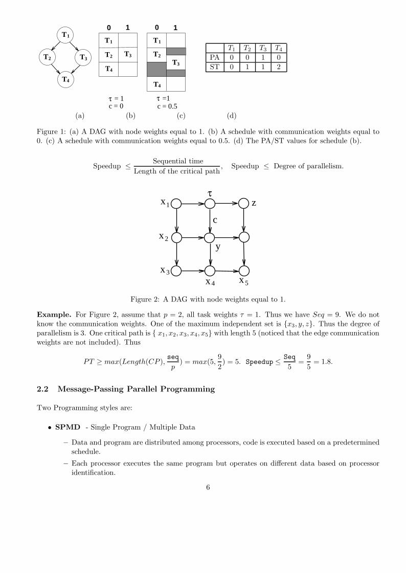
T1

T2 T3

T4

T1

T2 T3

T4

T1

T2

T3

T4

c = 0.5τ =1

c = 0τ = 1

10 0 1

T1 T2 T3 T4

PA 0 0 1 0ST 0 1 1 2

(a) (b) (c) (d)

Figure 1: (a) A DAG with node weights equal to 1. (b) A schedule with communication weights equal to0. (c) A schedule with communication weights equal to 0.5. (d) The PA/ST values for schedule (b).

Speedup ≤ Sequential timeLength of the critical path

, Speedup ≤ Degree of parallelism.

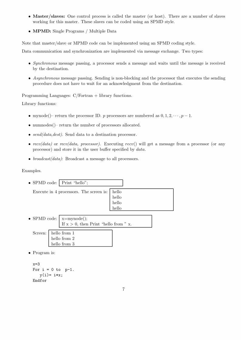
x2

x1

x3

x4 x5

τz

y

c

Figure 2: A DAG with node weights equal to 1.

Example. For Figure 2, assume that p = 2, all task weights τ = 1. Thus we have Seq = 9. We do notknow the communication weights. One of the maximum independent set is {x3, y, z}. Thus the degree ofparallelism is 3. One critical path is { x1, x2, x3, x4, x5} with length 5 (noticed that the edge communicationweights are not included). Thus

PT ≥ max(Length(CP ),seq

p) = max(5,

92) = 5. Speedup ≤ Seq

5=

95

= 1.8.

2.2 Message-Passing Parallel Programming

Two Programming styles are:

• SPMD - Single Program / Multiple Data

– Data and program are distributed among processors, code is executed based on a predeterminedschedule.

– Each processor executes the same program but operates on different data based on processoridentification.

6

• Master/slaves: One control process is called the master (or host). There are a number of slavesworking for this master. These slaves can be coded using an SPMD style.

• MPMD: Single Programs / Multiple Data

Note that master/slave or MPMD code can be implemented using an SPMD coding style.

Data communication and synchronization are implemented via message exchange. Two types:

• Synchronous message passing, a processor sends a message and waits until the message is receivedby the destination.

• Asynchronous message passing. Sending is non-blocking and the processor that executes the sendingprocedure does not have to wait for an acknowledgment from the destination.

Programming Languages: C/Fortran + library functions.

Library functions:

• mynode()– return the processor ID. p processors are numbered as 0, 1, 2, · · · , p − 1.

• numnodes()– return the number of processors allocated.

• send(data,dest). Send data to a destination processor.

• recv(data) or recv(data, processor). Executing recv() will get a message from a processor (or anyprocessor) and store it in the user buffer specified by data.

• broadcast(data): Broadcast a message to all processors.

Examples.

• SPMD code: Print “hello”;

Execute in 4 processors. The screen is: hellohellohellohello

• SPMD code: x=mynode();If x > 0, then Print “hello from ” x.

Screen: hello from 1hello from 2hello from 3

• Program is:

x=3For i = 0 to p-1.

y(i)= i*x;Endfor

7

SPMD code: int x, y, i;x=3;i=mynode();y=i*x;

or int x, y, i;i=mynode();if (i==0) then x=3; broadcast(x).else recv(x).y=i*x;

Libraries available for parallel programming using C/C++ or Fortran:

• PVM. Master/slaves programming style. The first widely adopted library for using a workstationcluster as a parallel machine.

• MPI. SPMD programming style. The most widely used message-passing standard for parallel pro-gramming. Available in all commercial parallel machines and workstation clusters.

PVM:

• A master program is regular C or Fortran code. It calls pvm spawn(Slave binary code, arguments)to create a slave process.

• The system spawns and executes slave Unix processes on different nodes of a parallel machine/workstationcluster.

• The master and slaves communicate using message-passing library functions (send,recv, broadcastetc).

2.3 Complexity analysis for parallel algorithms

How to Analyze Parallel Times. If a parallel program consists of separate phases of computation andcommunication.

PTp = Computation T ime + Communication T ime.

Communication cost for sending one message of size n between two nodes:

α + nβ

• α — the startup time, for handling a message at the sending processor (e.g. the packaging cost),plus the latency for the latency for a message to reach the destination.

• β — the data transmission speed between two processors (β=1/bandwidth).

• n - size of this message.

Example. Add n number on two computers. The first computer initially owns all numbers.

1. Computer 1 sends n/2 numbers to computer 2.

2. Both computers add n/2 numbers simultaneously.

3. Computer 2 sends its partial result back to computer 1.

4. Computer 1 adds the partial sums to produce the final result.

8

Assume that computation cost per operation is ω. Computation cost for Steps 2 and 4 is (n/2 + 1)ω.Communication cost for Steps 1 and 3 is α + n/2 ∗ β + α + β. Total parallel time is:

(n/2 + 1)ω + 2α + (n/2 + 1)β.

Approximation in analysis. The O notation for measuring space/time complexity:

• called big-oh: the order of magnitude.

• Example: f(x) = 4x2 + 2x + 12 is O(x2).

• Example: f(x) = 4x2 + 2xlogx + 12 is O(x2).

• Formal definition: f(x) = O(g(x)) iff there exists positive constants, c and x0 such that 0 ≤ f(x) ≤cg(x) for all x ≥ x0.

Approximation in cost analysis for parallel computing:

• You can drop insignificant terms during analysis.

• Example: Parallel time = 2 ∗ n2 + 3n log n ≈ 2 ∗ n2.

Empirical program evaluation. Measuring execution time through instrumentation:

• Add extra code in a program (e.g. clock(), time(), gettimeofday()).

• Measure the elapsed time between two points.

L1: time(&t1); /* start timer*/parallel code

L2: time(&t2); /* stop timer*/elapsed_time=difftime(t2,t1);...

Measure communication time. Use a ping-pong test for point-to-point communication.

At process 0.

L1: time(&t1);send(&x,P1)recv(&x,P1)

L2: time(&t2);elapsed_time=0.5*difftime(t2,t1);

At process 1.

recv(&x,P0)send(&x,P0)

9

3 Model-based Programming Methods

We can follow a specific parallelism model to program an application: 1) Embarrassingly parallel compu-tations. 2) Divide-and-conquer. 3) Pipelined computations.

3.1 Embarrassingly Parallel Computations

Computation can be divided and can be done independently on multiprocessors. Examples: Geometri-cal transformations of images. Mandelbrot set (image processing). Monte Carlo Methods for numericalcomputations.

3.1.1 Geometrical Transformations of Images

Given a 2D image (pixmap), each pixel is located at position (x,y):

• Shiftingx′ = x + ∆x; y′ = y + ∆y;

• Scalingx′ = x ∗ ∆x; y′ = y ∗ ∆y;

• Rotationx′ = x ∗ cosθ + y ∗ sinθ; y′ = −x ∗ cosθ + y ∗ sinθ;

• Clipping. (x,y) will be displayed only if

xl ≤ x ≤ xh; yl ≤ y ≤ yh;

Since operations performed on pixels are independent, parallel code can be designed as:

• A master holds an n × n image.

• p slaves are used to process an image.

• Each slave processes a portion of rows.

Master code:

• Tell each slave which rows to process .

• Wait to receive results from each slave. The result is a mapping (old pixel position, new pixelposition).

• Update the bitmap.

Slave code:

• Receive row numbers from the master that should be processed..

10

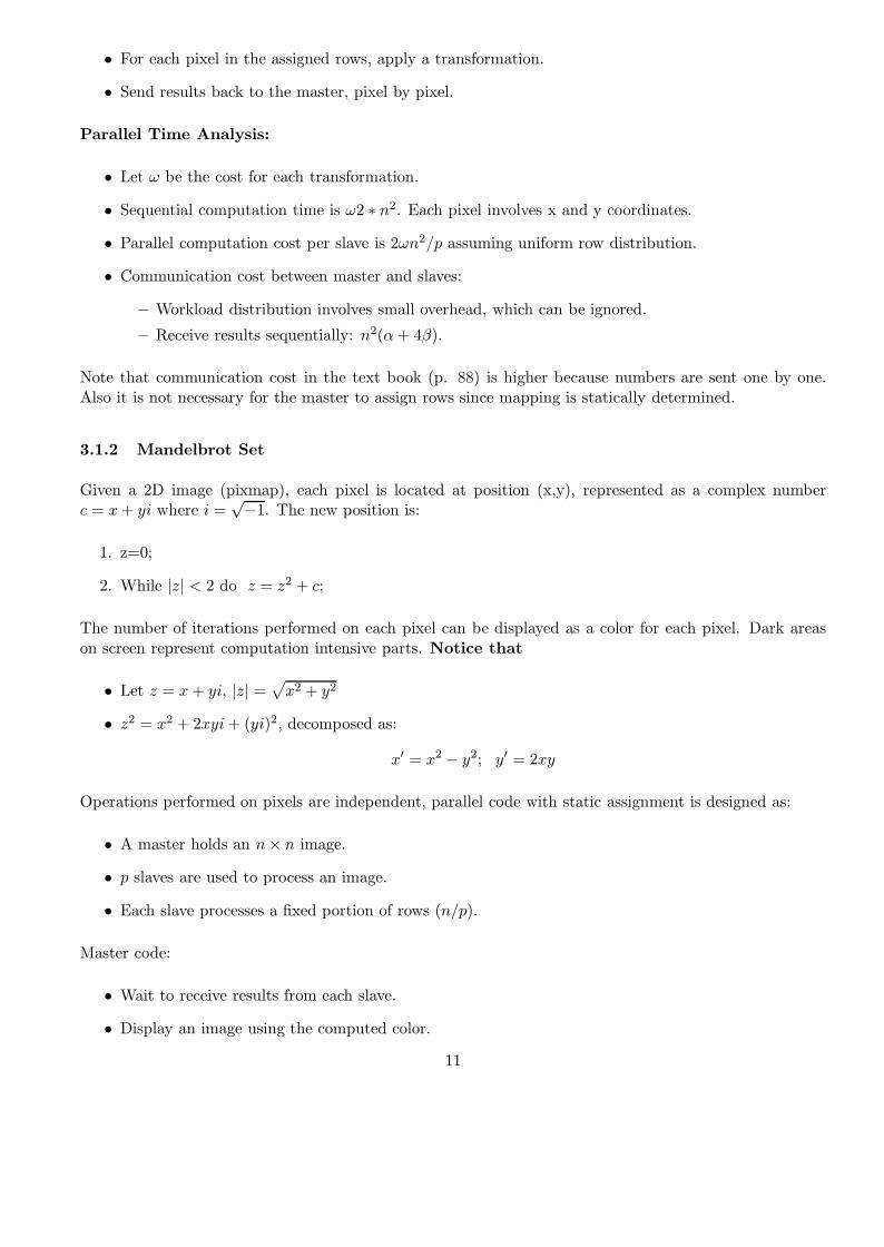
• For each pixel in the assigned rows, apply a transformation.

• Send results back to the master, pixel by pixel.

Parallel Time Analysis:

• Let ω be the cost for each transformation.

• Sequential computation time is ω2 ∗ n2. Each pixel involves x and y coordinates.

• Parallel computation cost per slave is 2ωn2/p assuming uniform row distribution.

• Communication cost between master and slaves:

– Workload distribution involves small overhead, which can be ignored.

– Receive results sequentially: n2(α + 4β).

Note that communication cost in the text book (p. 88) is higher because numbers are sent one by one.Also it is not necessary for the master to assign rows since mapping is statically determined.

3.1.2 Mandelbrot Set

Given a 2D image (pixmap), each pixel is located at position (x,y), represented as a complex numberc = x + yi where i =

√−1. The new position is:

1. z=0;

2. While |z| < 2 do z = z2 + c;

The number of iterations performed on each pixel can be displayed as a color for each pixel. Dark areason screen represent computation intensive parts. Notice that

• Let z = x + yi, |z| =√

x2 + y2

• z2 = x2 + 2xyi + (yi)2, decomposed as:

x′ = x2 − y2; y′ = 2xy

Operations performed on pixels are independent, parallel code with static assignment is designed as:

• A master holds an n × n image.

• p slaves are used to process an image.

• Each slave processes a fixed portion of rows (n/p).

Master code:

• Wait to receive results from each slave.

• Display an image using the computed color.

11

Slave code:

• For each pixel in the assigned rows, apply a transformation.

• Send results back to the master.

Computing costs among rows are non-uniform. Processor load may not be balanced.

Parallel code with dynamic assignment can balance load better. The basic idea is that master assigns rowsbased on slaves’ computation speed.

Master code:

• Assign one row per slave.

• Receive results from a slave (any slave) and assign another row to that slave. Repeat until all rowsare processed.

• Tell all slaves to stop. Display the results.

Slave code:

1. Receive a row from the master.

2. For each pixel in the assigned rows, apply a transformation.

3. Send results back to the master.

4. Go to 1 until a master sends a termination signal.

3.1.3 Monte Carlo Methods

Such a method uses random selections in calculations for numerical computing problems. Example: Howcan we compute an integral such as: ∫ 1

0

√1 − x2dx =

π

4?

A probabilistic method for such a problem:

∫ x2

x1

f(x)dx = limN→∞

N∑i=1

f(xi).

where xi is a random number between x1 and x2. The sequential code is:

sum=0;for (i=0; i<N; i++){

z = random_number(x1,x2);sum = sum + f(z);

}

Parallel Code:

12

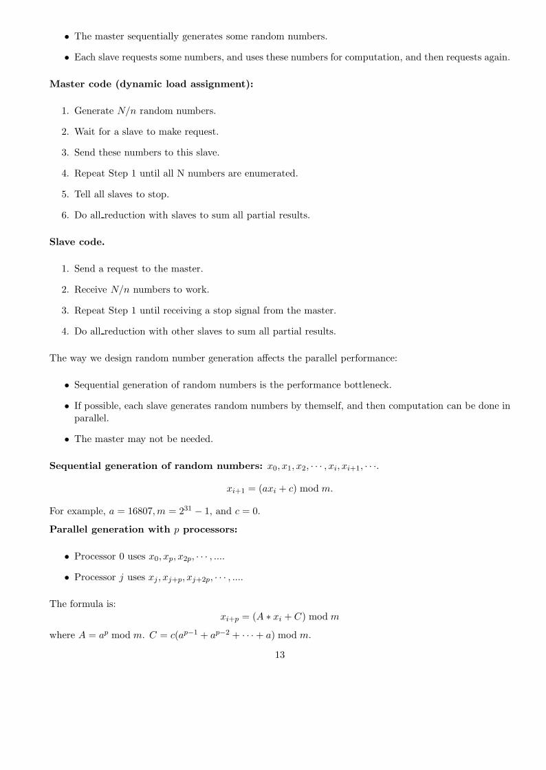
• The master sequentially generates some random numbers.

• Each slave requests some numbers, and uses these numbers for computation, and then requests again.

Master code (dynamic load assignment):

1. Generate N/n random numbers.

2. Wait for a slave to make request.

3. Send these numbers to this slave.

4. Repeat Step 1 until all N numbers are enumerated.

5. Tell all slaves to stop.

6. Do all reduction with slaves to sum all partial results.

Slave code.

1. Send a request to the master.

2. Receive N/n numbers to work.

3. Repeat Step 1 until receiving a stop signal from the master.

4. Do all reduction with other slaves to sum all partial results.

The way we design random number generation affects the parallel performance:

• Sequential generation of random numbers is the performance bottleneck.

• If possible, each slave generates random numbers by themself, and then computation can be done inparallel.

• The master may not be needed.

Sequential generation of random numbers: x0, x1, x2, · · · , xi, xi+1, · · ·.

xi+1 = (axi + c) mod m.

For example, a = 16807,m = 231 − 1, and c = 0.

Parallel generation with p processors:

• Processor 0 uses x0, xp, x2p, · · · , ....• Processor j uses xj , xj+p, xj+2p, · · · , ....

The formula is:xi+p = (A ∗ xi + C) mod m

where A = ap mod m. C = c(ap−1 + ap−2 + · · · + a) mod m.

13

3.2 Divide-and-Conquer

• Partitioning a problem into subproblems.

• Solve small problems first (possibly in parallel).

• Then solve the original problem.

• This divide-and-conquer process can be recursive.

Example: Add n numbers. Numerical Integration. N-body simulation problem.

3.2.1 Add n numbers

Master/slave version for adding n numbers with simple partitioning:

• Master distributes n/m numbers to each slave.

• Each of m slaves adds n/m numbers.

• Master collects m partial results of slaves and adds them together.

SPMD version:

• Assumes that each of m slaves holds n/m numbers.

• Each slave adds n/m numbers.

• Perform a global reduction to add partial results together. adds them together.

Summation with a tree structure Recursive divide-and-conquer (sequential code):

int add (int *s){if(numbers(s)<= 2) return (simple_add(s));Divide(s, s1, s2);part_sum1= add(s1);part_sum2= add(s2);return (part_sum1+part_sum2);

}

Parallel summation with a tree structure:

a1 a2 a3 a4 a5 a6 a7 a8

+

+

+

P0 P1 P2 P3

1 2 3 4

5 6

7

+ + + +

Schedule

1 2 3 4

5 6

7

14

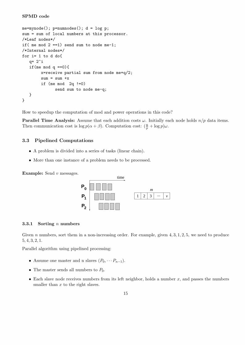
SPMD code

me=mynode(); p=numnodes(); d = log p;sum = sum of local numbers at this processor./*Leaf nodes*/if( me mod 2 ==1) send sum to node me-1;/*Internal nodes*/for i= 1 to d do{

q= 2^iif(me mod q ==0){

x=receive partial sum from node me+q/2;sum = sum +xif (me mod 2q !=0)

send sum to node me-q;}

}

How to speedup the computation of mod and power operations in this code?

Parallel Time Analysis: Assume that each addition costs ω. Initially each node holds n/p data items.Then communication cost is log p(α + β). Computation cost: (n

p + log p)ω.

3.3 Pipelined Computations

• A problem is divided into a series of tasks (linear chain).

• More than one instance of a problem needs to be processed.

Example: Send v messages.

P0

P1

P2

21 3 v...m

time

3.3.1 Sorting n numbers

Given n numbers, sort them in a non-increasing order. For example, given 4, 3, 1, 2, 5, we need to produce5, 4, 3, 2, 1.

Parallel algorithm using pipelined processing:

• Assume one master and n slaves (P0, · · ·Pn−1).

• The master sends all numbers to P0.

• Each slave node receives numbers from its left neighbor, holds a number x, and passes the numberssmaller than x to the right slaves.

15

SPMD code for slaves

me=mynode();no_stage= n-me-1;recv(x, me-1);for j=1 to stage

recv(newnumber, me-1);if( newnumber > x){

send(x, me+1);x=newnumber;

} else send(newnumber, me+1);

4 Transformation-based Parallel Programming

We discuss the basic program parallelization techniques in dependence analysis, program/data partitioningand mapping.

4.1 Dependence Analysis

Before executing a program in processors, we need to identify the inherent parallelism in this program. Inthis chapter, we discuss several graphical representations of program parallelism.

4.1.1 Basic dependence

We need to introduce the concept of dependence. We call a basic computation unit as a task. A task is aprogram fragment, which could be a basic assignment, a procedure or a logical test. A program consistsof a sequence of tasks. When tasks are executed in parallel on different processors, the relative executionorder of those tasks is different from the one in the sequential execution. It is mandatory to study ordersbetween tasks that must be followed so that the semantic of this program does not change during parallelexecution. For example:

S1 : x = a + bS2 : y = x + c

For this example, each statement is considered as a task. Assume statements are executed in separateprocessors. S2 needs to use the value of x defined by S1. If two processors share one memory, S1 has tobe executed first in one processor. The result of x is updated in the global memory. Then S2 can fetchx from the memory and start its execution. In a distributed environment, after the execution of S1, datax needs to be sent to the processor where S2 is executed. This example demonstrates the importance ofdependence relations between tasks. We formally define basic types of data dependence between tasks.

Definition: Let IN(T ) be the set of data items used by task T and OUT (T ) be the set of data itemsmodified by T .

• OUT (T1)⋂

IN(T2) �= ∅T2 is data flow-dependent (or called true-dependent) on T1. Example: S1 : A = x + B

S2 : C = A ∗ 3

16

• OUT (T1)⋂

OUT (T2) �= ∅T2 is output-dependent on T1. S1 : A = x + B

S2 : A = 3

• IN(T1)⋂

OUT (T2) �= ∅T2 is anti-dependent on T1. S1 : B = A + 3

S2 : A = 3

Coarse-grain dependence graph. Tasks operate on a set of data items of large sizes and perform alarge chunk of computations. An example of such a dependence graph is shown in Figure 3.

S1

S2

S3

flow

outputflow

flow anti

S1: A=f(X,B)

S2: C=g(A)

S3: A=h(A,C)

Figure 3: An example of a dependence graph. Functions f, g, h do not modify their input arguments.

4.1.2 Loop Parallelism

Loop parallelism can be modeled by the iteration space of a loop program which contains all iterations ofa loop and data dependence between iteration statements. An example is in Fig. 4.

For i= 1 to n

S i: a(i)=b(i)+c(i)

1D Loop:

S1 S2 Sn

For i= 1 to n Si: a(i)=a(i−1) +c(i) S1 S2 Sn

2D Loop:

For i = 1 to 3For j= 1 to 3

S i,j : X(i,j)=X(i,j−1)+1S11 S12 S13

S21 S22 S23

S31 S32 S33i

j

Figure 4: An example of a loop dependence graph (loop iteration space).

4.2 Program Partitioning

Purpose:

17

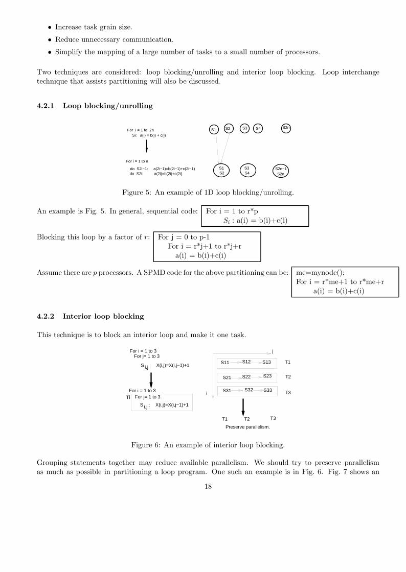
• Increase task grain size.

• Reduce unnecessary communication.

• Simplify the mapping of a large number of tasks to a small number of processors.

Two techniques are considered: loop blocking/unrolling and interior loop blocking. Loop interchangetechnique that assists partitioning will also be discussed.

4.2.1 Loop blocking/unrolling

For i = 1 to 2nSi: a(i) = b(i) + c(i)

For i = 1 to n

do S2i−1: a(2i−1)=b(2i−1)+c(2i−1)do S2i: a(2i)=b(2i)+c(2i)

S2nS2 S3 S4S1

S1S2

S3S4

S2n−1S2n

Figure 5: An example of 1D loop blocking/unrolling.

An example is Fig. 5. In general, sequential code: For i = 1 to r*pSi : a(i) = b(i)+c(i)

Blocking this loop by a factor of r: For j = 0 to p-1For i = r*j+1 to r*j+r

a(i) = b(i)+c(i)

Assume there are p processors. A SPMD code for the above partitioning can be: me=mynode();For i = r*me+1 to r*me+r

a(i) = b(i)+c(i)

4.2.2 Interior loop blocking

This technique is to block an interior loop and make it one task.


S i,j : X(i,j)=X(i,j−1)+1S11 S12 S13

S21 S22 S23

S31 S32 S33i

j


S i,j : X(i,j)=X(i,j−1)+1

Ti

T1 T2 T3

T1

T2

T3

Preserve parallelism.

Figure 6: An example of interior loop blocking.

Grouping statements together may reduce available parallelism. We should try to preserve parallelismas much as possible in partitioning a loop program. One such an example is in Fig. 6. Fig. 7 shows an

18

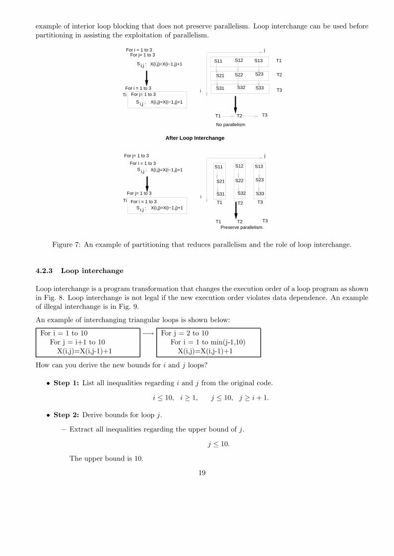
example of interior loop blocking that does not preserve parallelism. Loop interchange can be used beforepartitioning in assisting the exploitation of parallelism.

For i = 1 to 3

For j= 1 to 3

S i,j :S11 S12 S13

S21 S22 S23

S31 S32 S33i

j

For i = 1 to 3

For j= 1 to 3

S i,j :

Ti

T1 T2 T3

T1 T2 T3

X(i,j)=X(i−1,j)+1

X(i,j)=X(i−1,j)+1

After Loop Interchange


S i,j :S11 S12 S13

S21 S22 S23

S31 S32 S33i

j


S i,j :

Ti

T1 T2 T3

T1

T2

T3

X(i,j)=X(i−1,j)+1

X(i,j)=X(i−1,j)+1

No parallelism

Preserve parallelism.

Figure 7: An example of partitioning that reduces parallelism and the role of loop interchange.

4.2.3 Loop interchange

Loop interchange is a program transformation that changes the execution order of a loop program as shownin Fig. 8. Loop interchange is not legal if the new execution order violates data dependence. An exampleof illegal interchange is in Fig. 9.

An example of interchanging triangular loops is shown below:

For i = 1 to 10For j = i+1 to 10

X(i,j)=X(i,j-1)+1

−→ For j = 2 to 10For i = 1 to min(j-1,10)

X(i,j)=X(i,j-1)+1

How can you derive the new bounds for i and j loops?

• Step 1: List all inequalities regarding i and j from the original code.

i ≤ 10, i ≥ 1, j ≤ 10, j ≥ i + 1.

• Step 2: Derive bounds for loop j.

– Extract all inequalities regarding the upper bound of j.

j ≤ 10.

The upper bound is 10.

19

S11 S12 S13

S21 S22 S23

S31 S32 S33i

j

S11 S12 S13

S21 S22 S23

S31 S32 S33i

j

Execution order


S i,j :


S i,j :

Figure 8: Loop interchange re-orders execution.


S i,j :S11 S12 S13

S21 S22 S23

S31 S32 S33i

j

X(i,j)=X(i−1,j+1)+1


S i,j : X(i,j)=X(i−1,j+1)+1

Legal?

S11 S12 S13

S21 S22 S23

S31 S32 S33i

j

Execution order

Dependence

Figure 9: An illegal loop interchange.

20

– Extract all inequalities regarding the lower bound of j.

j ≥ i + 1.

The lower bound is 2 since i could be as low as 1.

• Step 3: Derive bounds for loop i when j value is fixed (now loop i is an inner loop).

– Extract all inequalities regarding the upper bound of i.

i ≤ 10, i ≤ j − 1.

The upper bound is min(10, j − 1).

– Extract all inequalities regarding the lower bound of i.

i ≥ 1.

The lower bound is 1.

4.3 Data Partitioning

For distributed memory architectures, data partitioning is needed when there is no enough space forreplication. Data structure is divided into data units and assigned to the local memories of the processors.A data unit can be a scalar variable, a vector or a submatrix block.

4.3.1 Data partitioning methods

1D array −→ 1D processors.

Assume that data items are counted from 0, 1, · · · n− 1, and processors are numbered from 0 to p− 1. Letr = n

p . Three common methods for a 1D array are depicted in Fig. 10.

r

0 1 2 3p 0 1 2 3 0 1 2 3 0 1 2 3 0 1 2 3p p 32103210

r r r r r r r r

(a) Block. (b) Cyclic. (c) Block cyclic.

Figure 10: Data partitioning schemes.

• 1D block. Data i is mapped to processor � ir �.

• 1D cyclic. Data i is mapped to processor i mod p.

• 1D block cyclic. First the array is divided into a set of units using block partitioning (block sizeb). Then these units are mapped in a cyclic manner to p processors. Data i is mapped to processor� i

b� mod p.


Data elements are counted as (i, j) where 0 ≤ i, j ≤ · · ·n − 1. Processors are numbered from 0 to p − 1.Let r = n

p .21

• Row-wise block. Data (i, j) is mapped to processor � ir �.

• Column-wise block. Data (i, j) is mapped to processor � jr �.

Proc0 1 2 3

Proc 0

Proc 1

Proc 2

Proc 3

Figure 11: The left is the column-wise block and the right is the row-wise block.

• Row-wise cyclic Data (i, j) is mapped to processor i mod p.

• Other partitioning. Column-wise cyclic, Column-wise block cyclic. Row-wise block cyclic.


Data elements are counted as (i, j) where 0 ≤ i, j ≤ · · · n − 1. Processors are numbered as (s, t) where0 ≤ s, t ≤ · · · q − 1 where q =

√p. Let r = n

q .

• (Block,Block). Data (i, j) is mapped to processor (� ir �, � j

r �)• (Cyclic,Cyclic). Data (i, j) is mapped to processor (i mod q, j mod q).

0 1 2 3

0

1

2

3

(0,0) (0,1) (0,2) (0,3)Proc Proc Proc Proc 0 1 2 3 0 1 2 3 0 1 2 3

012301230123

(0,3)Processor

Figure 12: The left is the 2D block mapping (block,block) and the right is the 2D cyclic mapping(cyclic,cyclic).

• Other partitioning. (Block, Cyclic), (Cyclic, Block), (Block cyclic, Block cyclic).

4.3.2 Consistency between program and data partitioning

Given a computation partitioning and processor mapping, there are several choices available for data parti-tioning and mapping. How can we make a good choice of data partitioning and mapping? For distributedmemory architectures large grain data partitioning is preferred because there is a high communication

22

startup overhead in transferring a small size data unit. If a task requires to access a large number ofdistinct data units and data units are evenly distributed among processors, then there will be substantialcommunication overhead in fetching a large number of non-local data items for executing this task. Thusthe following rule of thumb can be used to guide the design of program and data partitioning:

Consistency. The program partitioning and data partitioning are consistent if sufficient par-allelism is provided by partitioning and at the same time the number of distinct units accessedby each task is minimized.

The following rule is a simple heuristic used in determining data and program mapping.

“Owner computes rule”: If a computation statement x modifies a data item i, then theprocessor that owns data item i executes statement x.

For example, sequential code: For i = 0 to r*p-1Si : a(i) = 3.

Blocking this loop by a factor of r For j = 0 to p-1For i = r*j to r*j+r-1

a(i) = 3.

Assume there are p processors. SPMD code is: me=mynode();For i = r*me to r*me+r-1

a(i) = 3.

Data array a(i) are distributed to processors such that if processor x executes a(i) = 3, then a(i) is assignedto processor x. For example, we let processor 0 own data a(0), a(1), · · · , a(r − 1). Otherwise if processor0 does not have a(0), this processor needs to allocate some temporal space to perform a(0) = 3 and sendthe result back the processor that owns a(0), which leads to a certain amount of communication overhead.

The above SPMD code is for block mapping. For cyclic mapping, the code is:

me=mynode();For i = me to r*p-1 step-size p

a(i) = 3.

A more general SPMD code structure for an arbitrary processor mapping method proc map(i) (but withmore code overhead) is

me=mynode();For i =0 to rp-1

if ( proc map(i) == me) a(i) = 3.

For block mapping, proc map(i) = � ir �. For cyclic mapping, proc map(i) = i mod p.

4.3.3 Data indexing between global space and local space

There is one more problem with the previous program: statement “a(i)=3” uses “i” as the index functionand the value of i is in a range from 0 to r ∗ p − 1. When a processor allocates r units, there is a needto translate the global index i to a local index which accesses the local memory at that processor. This isdepicted in Fig.13. The correct code structure is shown below.

23

int a[r];me=mynode();For i =0 to rp-1

if ( proc map(i) == me) a(local(i)) = 3.

For block mapping, local(i) = i mod r. For cyclic mapping, local(i) = � ip�.

A

0 1 2 0 1 2

Local array, Proc 0 Local array, Proc 1

0 1 2 3 4 5

Figure 13: Global data vs local data index.

In summary, given data item i (i starts from 0).

• 1D Block.Processor ID: proc map(i) = � i

r �.Local data address: Local(i) = i mod r.

An example of mapping with p=2 and r=3 is:

Proc 0 Proc 10 → 0 3 → 01 → 1 4 → 12 → 2 5 → 2

• 1D Cyclic.Processor ID: proc map(i) = i mod p.

Local data address: Local(i) = � ip�.

An example of cyclic mapping with p=2 is:

proc 0 proc 10 → 0 1 → 02 → 1 3 → 14 → 2 5 → 26 → 3

4.4 A summary on program parallelization

The process of program parallelization is depicted in Figure 14 and we will demonstrate this process inparallelizing following scientific computing algorithms.

• Matrix-vector multiplication.

• Matrix-matrix multiplication.

• Direct methods for solving a linear equation. e.g. Gaussian Elimination.

• Iterative methods for solving a linear equation. e.g. Jacobi.

• Finite-difference methods for differential equations.

24

Program

CodePartitioning

DataPartitioning

dependenceTasks + Data

mappingscheduling

mapping

P processors P processors

parallel code

Figure 14: The process of program parallelization.

5 Matrix Vector Multiplication

Problem: y = A ∗ x where A is a n × n matrix and x is a column vector of dimension n.

Sequential code: for i = 1 to n doyi = 0;for j = 1 to n do

yi = yi + ai,j ∗ xj ;Endfor

Endfor

An example:

⎛⎜⎝ 1 2 3

4 5 67 8 9

⎞⎟⎠ ∗

⎛⎜⎝ 1

23

⎞⎟⎠ =

⎛⎜⎝ 1 ∗ 1 + 2 ∗ 2 + 3 ∗ 3

4 ∗ 1 + 5 ∗ 2 + 6 ∗ 37 ∗ 1 + 8 ∗ 2 + 9 ∗ 3

⎞⎟⎠ =

⎛⎜⎝ 14

3250

⎞⎟⎠

The sequential complexity is 2n2ω where ω is the time for an addition or multiplication.

Partitioned code: for i = 1 to n doSi : yi = 0;

for j = 1 to n doyi = yi + ai,j ∗ xj ;

EndforEndfor

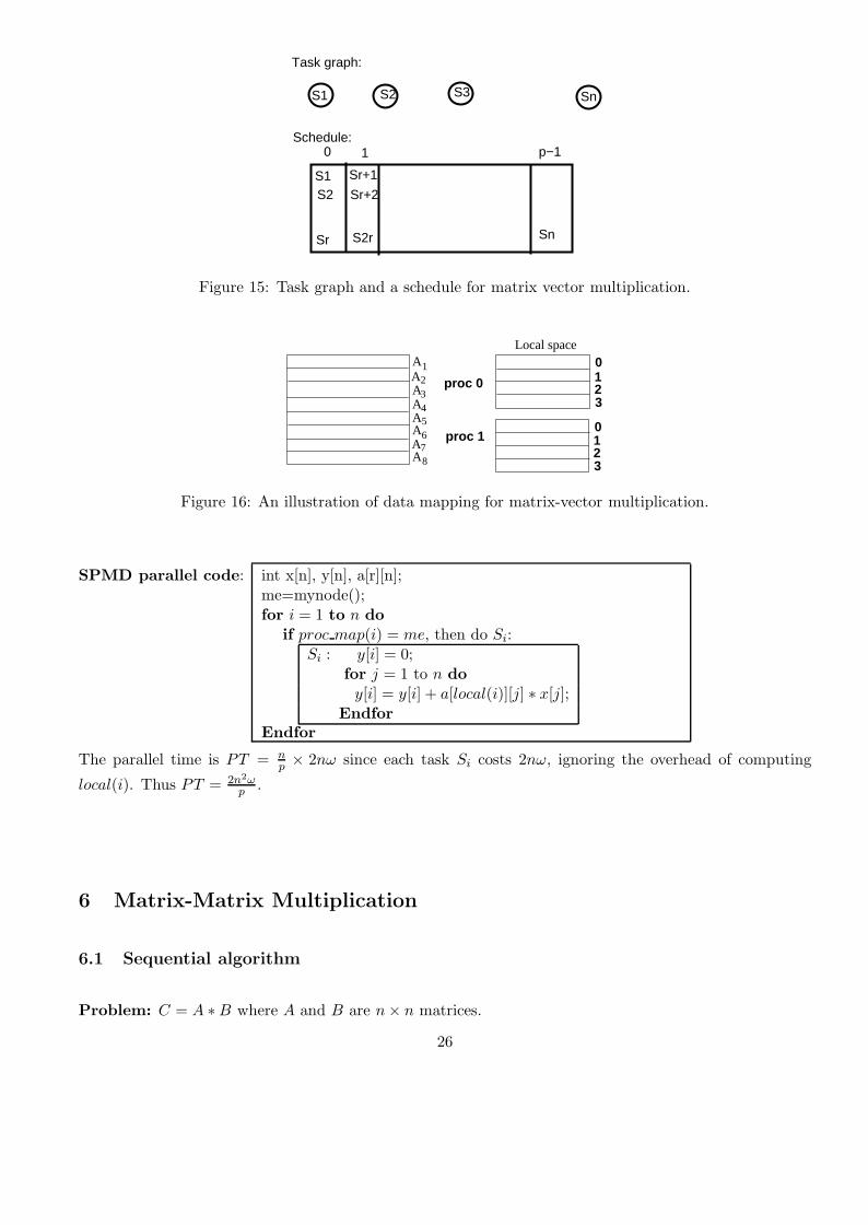
Dependence task graph is shown in Fig. 15.

Task schedule on p processors is shown in Fig. 15.

Mapping function of tasks Si. For the above schedule: proc map(i) = � i−1r � where r = n

p .Data partitioning based on the above schedule: matrix A is divided into n rows A1, A2, · · ·An.

Data mapping: Row Ai is mapped to processor proc map(i), the same as task i. The indexing functionis: local(i) = (i − 1) mod r. Vectors x and y are replicated to all processors.

25

S1 S2 S3 Sn

Task graph:

Schedule:

S1S2

Sr

Sr+1

S2r Sn

Sr+2

0 1 p−1

Figure 15: Task graph and a schedule for matrix vector multiplication.

A1A2A3A4A5A6A7A8

proc 1

proc 0

0123

0123

Local space

Figure 16: An illustration of data mapping for matrix-vector multiplication.

SPMD parallel code: int x[n], y[n], a[r][n];me=mynode();for i = 1 to n do

if proc map(i) = me, then do Si:Si : y[i] = 0;

for j = 1 to n doy[i] = y[i] + a[local(i)][j] ∗ x[j];

EndforEndfor

The parallel time is PT = np × 2nω since each task Si costs 2nω, ignoring the overhead of computing

local(i). Thus PT = 2n2ωp .

6 Matrix-Matrix Multiplication

6.1 Sequential algorithm

Problem: C = A ∗ B where A and B are n × n matrices.

26

Sequential code: for i = 1 to n dofor j = 1 to n do

sum = 0;for k = 1 to n do

sum = sum + a(i, k) ∗ b(k, j);Endforc(i, j) = sum;

EndforEndfor

An example: (1 23 4

)∗(

5 76 8

)=

(1 ∗ 5 + 2 ∗ 6 1 ∗ 7 + 2 ∗ 83 ∗ 5 + 4 ∗ 6 3 ∗ 7 + 4 ∗ 8

)

Time Complexity. Each multiplication or addition counts one time unit ω.

No of operations =n∑

i=1

n∑j=1

n∑k=1

2ω = 2n3ω

6.2 Parallel algorithm with sufficient memory

Partitioned code: for i = 1 to n doTi : for j = 1 to n do

sum = 0;for k = 1 to n do

sum = sum + a(i, k) ∗ b(k, j);Endforc(i, j) = sum;

EndforEndfor

Since tasks Ti (1 ≤ i ≤ n) are independent, we use the following mapping for the parallel code:

• Matrix A is partitioned using row-wise block mapping

• Matrix C is partitioned using row-wise block mapping

• Matrix B is duplicated to all processors

• Task Ti is mapped to the processor of row i in matrix A.

The SPMD code with parallel time 2n3ω/p is: For i = 1 to nif proc map(i)==me do Ti;

Endfor

A more detailed description of the algorithm is:

27

for i = 1 to n doif proc map(i)==me do

for j = 1 to n dosum = 0;for k = 1 to n do

sum = sum + a(local(i), k) ∗ b(k, j);Endforc(local(i), j) = sum;

Endforendif

Endfor

6.3 Parallel algorithm with 1D partitioning

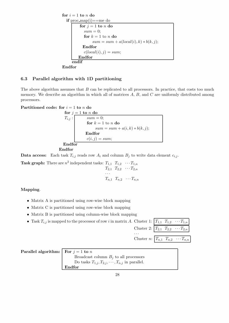
The above algorithm assumes that B can be replicated to all processors. In practice, that costs too muchmemory. We describe an algorithm in which all of matrices A, B, and C are uniformly distributed amongprocessors.

Partitioned code: for i = 1 to n dofor j = 1 to n doTi,j : sum = 0;

for k = 1 to n dosum = sum + a(i, k) ∗ b(k, j);

Endforc(i, j) = sum;

EndforEndfor

Data access: Each task Ti,j reads row Ai and column Bj to write data element ci,j.

Task graph: There are n2 independent tasks: T1,1 T1,2 · · ·T1,n

T2,1 T2,2 · · ·T2,n

· · ·Tn,1 Tn,2 · · · Tn,n

Mapping.

• Matrix A is partitioned using row-wise block mapping

• Matrix C is partitioned using row-wise block mapping

• Matrix B is partitioned using column-wise block mapping

• Task Ti,j is mapped to the processor of row i in matrix A. Cluster 1: T1,1 T1,2 · · ·T1,n

Cluster 2: T2,1 T2,2 · · ·T2,n

· · ·Cluster n: Tn,1 Tn,2 · · ·Tn,n

Parallel algorithm: For j = 1 to nBroadcast column Bj to all processorsDo tasks T1,j, T2,j , · · · , Tn,j in parallel.

Endfor

28

Parallel time analysis. Each multiplication or addition counts one time unit ω. Each task Ti,j costs2nω. Also we assume that each broadcast costs (α + βn) log p.

PT =n∑

j=1

((α + βn) log p +n

p2nω) = n(α + βn) log p +

2n3ω

p.

6.4 Fox’s algorithm for 2D data partitioning

This algorithm is similar to the Cannon’s algorithm described in the text book Chapter 10.2.4.

Naturally another option we have for program partitioning is to treat each interior statement as one task.Let us first ignore the initialization statement. We have the following partitioning.

for i = 1 to n dofor j = 1 to n do

for k = 1 to n doTi,j,k : ci,j = ci,j + ai,k ∗ bk,j;

EndforEndfor

EndforThen the iteration space is 3D. All tasks Ti,j,k (1 ≤ k ≤ n) that modify the same ci,j will have a chaindependence, which corresponds to a summation of n terms for ci,j. There are no dependence between thosechains.

The Fox’s algorithm is used to support 2D block partitioning of matrices A, B and C. This algorithmrequires a re-organization of the sequential code. There are two basic ideas: reordering the sequentialaddition and submatrix-based partitioning.

6.4.1 Reorder the sequential additions.

We examine the summation sequence for each result element ci,j,

ci,j = ai,1 ∗ b1,j + aj,2 ∗ b2,j + · · · + ai,n ∗ bn,j.

It can be re-ordered as:

ci,j = ai,i ∗ bi,j + ai,i+1 ∗ bi+1,j + · · · + ai,n ∗ bn,j + ai,1 ∗ b1,j + aj,2 ∗ b2,j + · · · + ai,i−1 ∗ bi−1,j.

i.e.

ci,j =n∑

k=1

ai,(i+k−2) mod n+1 ∗ b(i+k−2) mod n+1,j.

Assume that we use a 2D data mapping on n × n processors. Processor (i, j) owns data ai,j, bi,j and ci,j .We will execute the computation for ci,j in n stages. At stage k (k = 1, · · · , n), for all 1 ≤ i, j ≤ n, do

ci,j = ci,j + ai,(i+k−2) mod n+1 ∗ b(i+k−2) mod n+1,j

We use an example for 3 × 3 processors to demonstrate the computation sequence.⎡⎢⎣ c11 = a11 ∗ b11 c12 = a11 ∗ b12 c13 = a11 ∗ b13

c21 = a22 ∗ b21 c22 = a22 ∗ b22 c23 = a22 ∗ b23

c31 = a33 ∗ b31 c32 = a33 ∗ b32 c33 = a33 ∗ b33

⎤⎥⎦

k=1

=⇒⎡⎢⎣ c11+ = a12 ∗ b21 c12+ = a12 ∗ b22 c13+ = a12 ∗ b23

c21+ = a23 ∗ b31 c22+ = a23 ∗ b32 c23+ = a23 ∗ b33

c31+ = a31 ∗ b11 c32+ = a31 ∗ b12 c33+ = a31 ∗ b13

29

=⇒⎡⎢⎣ c11+ = a13 ∗ b31 c12+ = a13 ∗ b32 c13+ = a13 ∗ b33

c21+ = a21 ∗ b11 c22+ = a21 ∗ b12 c23+ = a21 ∗ b13

c31+ = a32 ∗ b21 c32+ = a32 ∗ b22 c33+ = a32 ∗ b23

⎤⎥⎦

k=3

Then we examine what elements of a are used during the above 3 stages so we can determine the commu-nication patterns.

⎡⎢⎣ a11 a11 a11

a22 a22 a22

a33 a33 a33

⎤⎥⎦

k=1

=⇒⎡⎢⎣ a12 a12 a12

a23 a23 a23

a31 a31 a31

⎤⎥⎦

k=2

=⇒⎡⎢⎣ a13 a13 a13

a21 a21 a21

a32 a32 a32

⎤⎥⎦

k=3

Thus the communication pattern is that at each stage, ai,(i+k−2) mod n+1 is broadcasted to every processorin row i. We also examine what elements of b are used for each grid point at each stage.

⎡⎢⎣ b11 b12 b13

b21 b22 b23

b31 b32 b33

⎤⎥⎦

k=1

=⇒⎡⎢⎣ b21 b22 b23

b31 b32 b33

b11 b12 b13

⎤⎥⎦

k=2

=⇒⎡⎢⎣ b31 b32 b33

b11 b12 b13

b21 b22 b23

⎤⎥⎦

k=3

For b, studying the element movement of column 1 from Stage 1, 2 to 3, we can observe that essentially aring pipelining for all-all broadcast is conducted in every column direction.

Parallel algorithm:

For k = 1 to nOn each processor (i, j), set t = (k + i − 2) mod n + 1.At each row, ai,t at processor (i, t) is broadcasted to other processors in the same row (i, j) where

1 ≤ j ≤ n.Do ci,j = ci,j + ai,t ∗ bt,j in parallel for all processors.Every processor (i,j) sends bi,t to processor (i − 1, j).

Endfor

6.4.2 Submatrix partitioning for block-based matrix multiplication

In practice, the number of processors is much less than n2. Also it does not make sense to utilize n2

processors since the code suffers too much communication overhead for fine-grain computation. To increasethe granularity of computation, we map the n × n grid to processors using the 2D block method.

First we partition all matrices (A,B,C of size n×n) in a submatrix style. Each processor (i, j) is assigneda submatrix of size n/q × n/q where q =

√p. Let r = n/q. The submatrix partitioning of A can be

demonstrated using the following example with n = 4 and q = 2.

A =

⎛⎜⎜⎜⎝

a11 a12 a13 a1n

a21 a22 a23 a24

a31 a32 a33 a34

a41 a42 a43 a44

⎞⎟⎟⎟⎠ =⇒

(A11 A12

A21 A22

)

where

A11 =

(a11 a12

a21 a22

), A12 =

(a13 a14

a23 a24

), A21 =

(a31 a32

a41 a42

), A22 =

(a33 a34

a43 a44

).

Then the sequential algorithm can be re-organized as

30

for i = 1 to q dofor j = 1 to q do

Ci,j = 0;for k = 1 to q do

Ci,j = Ci,j + Ai,k ∗ Bk,j;Endfor

EndforEndfor

Then we use the same idea of re-ordering:

Ci,j = Ai,i ∗ Bi,j + Ai,i+1 ∗ Bi+1,j + · · · + Ai,n ∗ Bn,j + Ai,1 ∗ B1,j + Aj,2 ∗ B2,j + · · · + Ai,i−1 ∗ Bi−1,j.

Parallel algorithm:

For k = 1 to qOn each processor (i, j), t = (k + i − 2) mod q + 1.At each row, Ai,t at processor (i, t) is broadcasted to other processors in the same row (i, j) where

1 ≤ j ≤ q.Do Ci,j = Ci,j + Ai,t ∗ Bt,j in parallel for all processors.Every processor (i,j) sends Bi,t to processor (i − 1, j).

Endfor

Parallel time analysis. A submatrix multiplication (Ai,t ∗ Bt,j) costs 2r3ω. A submatrix addition costsr2ω. Each inner most statement costs 2r3ω. Also we assume that each broadcast of a submatrix costs(α + βr2) log q.

PT =q∑

k=1

((α+βr2)(1+log q)+2r3ω) = q(α+β(n/q)2)(1+log q)+2(n/q)3ω = (√

pα+βn2

√p)(1+log

√p)+

2n3ω

p.

This algorithm has communication overhead much smaller than the 1D algorithm presented in the previoussubsection.

6.5 How to produce block-based matrix multiplication code

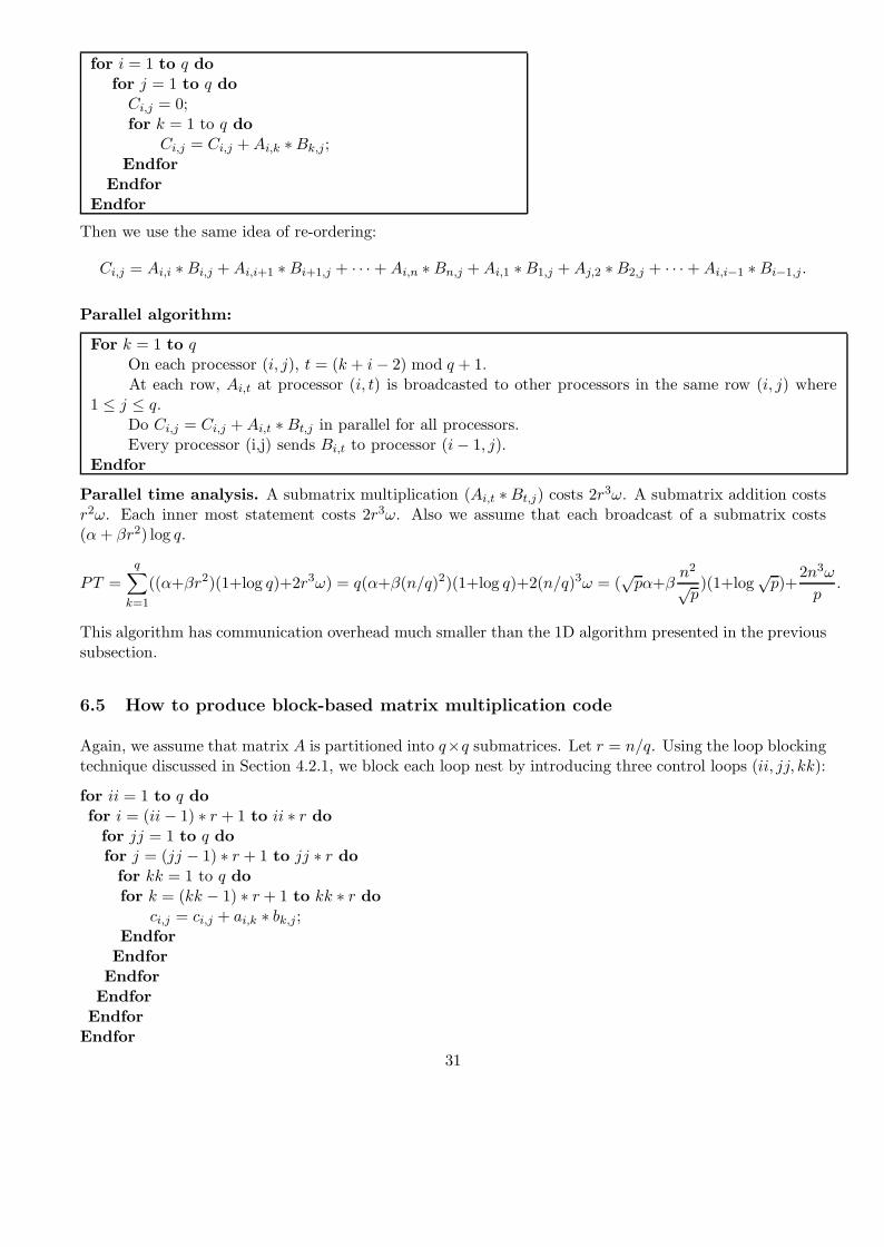
Again, we assume that matrix A is partitioned into q×q submatrices. Let r = n/q. Using the loop blockingtechnique discussed in Section 4.2.1, we block each loop nest by introducing three control loops (ii, jj, kk):

for ii = 1 to q dofor i = (ii − 1) ∗ r + 1 to ii ∗ r do

for jj = 1 to q dofor j = (jj − 1) ∗ r + 1 to jj ∗ r do

for kk = 1 to q dofor k = (kk − 1) ∗ r + 1 to kk ∗ r do

ci,j = ci,j + ai,k ∗ bk,j;Endfor

EndforEndfor

EndforEndfor

Endfor31

Then we use the loop interchange technique discussed in Section 4.2.3:

for ii = 1 to q dofor jj = 1 to q dofor kk = 1 to q dofor i = (ii − 1) ∗ r + 1 to ii ∗ r dofor j = (jj − 1) ∗ r + 1 to jj ∗ r dofor k = (kk − 1) ∗ r + 1 to kk ∗ r do

ci,j = ci,j + ai,k ∗ bk,j;Endfor

EndforEndfor

EndforEndfor

EndforThe inner three loops access three submatrices in A,B, and C. The above code is the same as the block-based code we have used in the previous subsection, excluding the initialization of matrix C.

7 Gaussian Elimination for Solving Linear Systems

7.1 Gaussian Elimination without Partial Pivoting

7.1.1 The Row-Oriented GE sequential algorithm

The Gaussian Elimination method for solving linear system Ax = b is listed below. Assume that columnn + 1 of A stores column b. Loop k controls the elimination steps. Loop i controls i-th row accessing andloop j controls j-th column accessing.

Forward Elimination: For k = 1 to n − 1For i = k + 1 to n

ai,k = ai,k/ak,k;For j = k + 1 to n + 1

ai,j = ai,j − ai,k ∗ ak,j;Endfor

EndforEndfor

Notice that since the lower triangle matrix elements become zero after elimination, their space is used tostore multipliers ( ai,k = ai,k/ak,k).

Backward Substitution: Note that xi uses the space of ai,n+1. For i = n to 1For j = i + 1 to n

xi = xi − ai,j ∗ xj ;Endfor

xi = xi/ai,i;Endfor

An example: Given the following matrix system:

32

(1) 4x1 − 9x2 + 2x3 = 2(2) 2x1 − 4x2 + 4x3 = 3(3) −x1 + 2x2 + 2x3 = 1

We eliminate the coefficients of x1 for equations (2) and (3) and make them zero.

(2)-(1)*24 : 0.5x2 + 3x3 = 2 (4)

(3)-(1)*-14 : −1

4x2 + 52x3 = 3

2 (5)

Then we eliminate the coefficients of x2 for equation (5).

(5)-(4)*-12 : 4x3 = 5

2

Now we have an upper triangular system:4x1 − 9x2 + 2x3 = 2

12x2 + 3x3 = 2

4x3 = 52

Given this upper triangular system, backward substitution performs the following operations:

x3 = 58

x2 = 2−3x312

= 14

x1 = 2+9x2−2x34 = 3

4

The forward elimination process can be expressed using an augmented matrix (A | b) where b is treated asthe n+1 column of A.

⎛⎜⎝ 4 −9 2 2

2 −4 4 3−1 2 2 1

⎞⎟⎠

(2)=(2)−(1)∗ 24

(3)=(3)−(1)∗−14=⇒⎛⎜⎝ 4 −9 2 2

0 12 3 2

0 −14

52

32

⎞⎟⎠ −→

⎛⎜⎝ 4 −9 2 2

0 1/2 3 20 0 4 5/2

⎞⎟⎠

Time complexity: Each of division, multiplication and subtraction counts one time unit ω.

#Operations in forward elimination:

n−1∑k=1

n∑i=k+1

⎛⎝1 +

n+1∑j=k+1

2

⎞⎠ω =

n−1∑k=1

n∑i=k+1

(2(n − k) + 3)ω ≈ 2ωn−1∑k=1

(n − k)2 ≈ 2n3

3ω

#Operations in backward substitution:

n∑i=1

(1 +n∑

j=i+1

2)ω ≈ 2ωn∑

i=1

(n − i) ≈ n2ω

Thus the total number of operations is about 2n3

3 ω. The total space needed is about n2 double-precisionnumbers.

7.1.2 The row-oriented parallel algorithm

A program partitioning for the forward elimination part is list below (Referece: Text book chapter10.3.3).

33

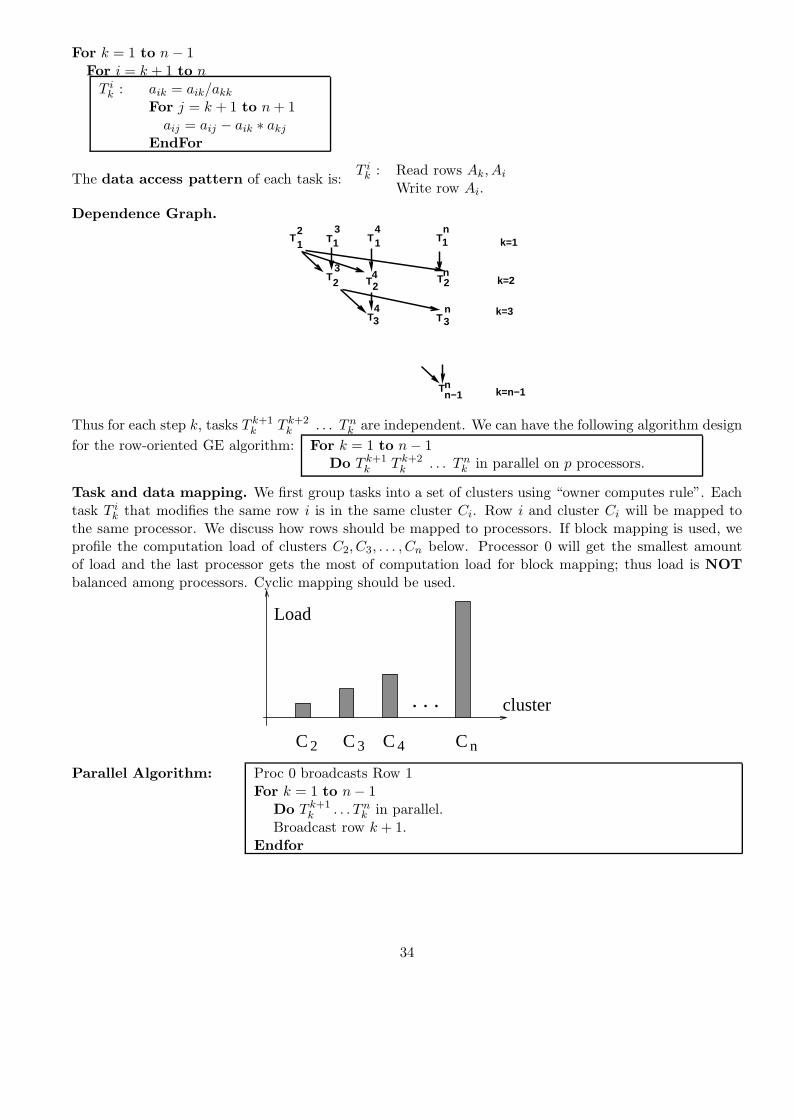
For k = 1 to n − 1For i = k + 1 to n

T ik : aik = aik/akk

For j = k + 1 to n + 1aij = aij − aik ∗ akj

EndFor

The data access pattern of each task is:T i

k : Read rows Ak, Ai

Write row Ai.

Dependence Graph.

T12

T13

T14

T1n

T23

T2n

T24

T34

Tn−1n

T3n

k=1

k=2

k=n−1

k=3

Thus for each step k, tasks T k+1k T k+2

k . . . T nk are independent. We can have the following algorithm design

for the row-oriented GE algorithm: For k = 1 to n − 1Do T k+1

k T k+2k . . . T n

k in parallel on p processors.

Task and data mapping. We first group tasks into a set of clusters using “owner computes rule”. Eachtask T i

k that modifies the same row i is in the same cluster Ci. Row i and cluster Ci will be mapped tothe same processor. We discuss how rows should be mapped to processors. If block mapping is used, weprofile the computation load of clusters C2, C3, . . . , Cn below. Processor 0 will get the smallest amountof load and the last processor gets the most of computation load for block mapping; thus load is NOTbalanced among processors. Cyclic mapping should be used.

. . .

Load

C C C

cluster

C2 3 4 n

Parallel Algorithm: Proc 0 broadcasts Row 1For k = 1 to n − 1

Do T k+1k . . . T n

k in parallel.Broadcast row k + 1.

Endfor

34

SPMD Code: me=mynode();For i = 1 to n

if proc map(i)==me, initialize Row i;EndforIf proc map(1)==me, broadcast Row 1 else receive it;For k = 1 to n − 1

For i = k + 1 to nIf proc map(i)==me, do T i

k.EndForIf proc map(k+1)==me, then broadcast Row k + 1 else receive it.

EndFor

7.1.3 The column-oriented algorithm

The column-oriented algorithm essentially interchanges loops i and j of the GE program in Section 7.1.1.

Forward elimination part:

For k = 1 to n − 1For i = k + 1 to n

ai,k = ai,k/ak,k

EndForFor j = k + 1 to n + 1

For i = k + 1 to nai,j = ai,j − ai,k ∗ ak,j

EndForEndFor

EndFor

Given the first step of forward elimination in the previous example,⎛⎜⎝ 4 −9 2 2

2 −4 4 3−1 2 2 1

⎞⎟⎠

(2)=(2)−(1)∗ 24

(3)=(3)−(1)∗−14=⇒⎛⎜⎝ 4 −9 2 2

0 12 3 2

0 −14

52

32

⎞⎟⎠

One can mark the data access (writing) sequence for row-oriented elimination below. Notice that 1computes and stores the multiplier 2

4 and 5 stores −14 .⎛

⎜⎝ 1 2 3 45 6 7 8

⎞⎟⎠

Then the data writing sequence for column-oriented elimination is:⎛⎜⎝ 1 3 5 7

2 4 6 8

⎞⎟⎠

Notice that 1 computes and stores the multiplier 24 and 2 stores −1

4 .

35

Column-oriented backward substitution. We change the loops of i and j in the row-oriented backwardsubstitution code. Notice again that column n + 1 stores the solution vector x.

For j = n to 1xj = xj/aj,j;For i = j − 1 to 1xi = xi − ai,jxj ;

EndforEndFor

For example, given a upper triangular system:4x1 − 9x2 + 2x3 = 2

0.5x2 + 3x3 = 24x3 = 5

2 .

The row-oriented algorithm performs:

x3 = 58

x2 = 2 − 3x3

x2 = x20.5

x1 = 2 + 9x2

x1 = x1 − 2x3

x1 = x14 .

The column-oriented algorithm performs:

x3 = 58

x2 = 2 − 3x3

x1 = 2 − 2x3

x2 = x20.5

x1 = x1 + 9x2

x1 = x14 .

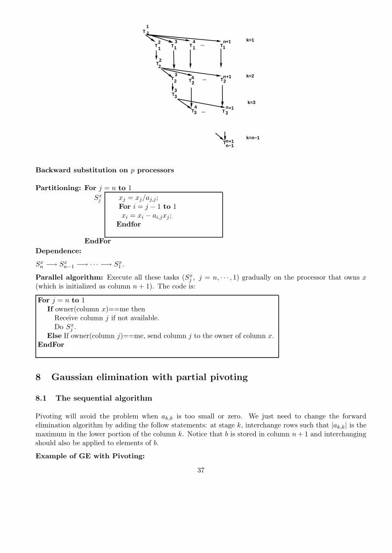
Partitioned forward elimination: For k = 1 to n − 1T k

k : For i = k + 1 to naik = aik/akk

EndforFor j = k + 1 to n + 1

T jk : For i = k + 1 to n

aij = aij − aik ∗ akj

EndforEndfor

EndforTask graph:

36

T12

T13

T14

T1n k=1

T23

T2n

T24 k=2

T34

Tn−1n

T3n

k=n−1

k=3

T 11

T22

+1

+1

+1

T33

...

...

...

+1

Backward substitution on p processors

Partitioning: For j = n to 1Sx

j xj = xj/aj,j;For i = j − 1 to 1xi = xi − ai,jxj ;

Endfor

EndForDependence:

Sxn −→ Sx

n−1 −→ · · · −→ Sx1 .

Parallel algorithm: Execute all these tasks (Sxj , j = n, · · · , 1) gradually on the processor that owns x

(which is initialized as column n + 1). The code is:

For j = n to 1If owner(column x)==me then

Receive column j if not available.Do Sx

j .Else If owner(column j)==me, send column j to the owner of column x.

EndFor

8 Gaussian elimination with partial pivoting

8.1 The sequential algorithm

Pivoting will avoid the problem when ak,k is too small or zero. We just need to change the forwardelimination algorithm by adding the follow statements: at stage k, interchange rows such that |ak,k| is themaximum in the lower portion of the column k. Notice that b is stored in column n + 1 and interchangingshould also be applied to elements of b.

Example of GE with Pivoting:

37

⎛⎜⎝ 0 1 1

3 2 −31 5 −1

∣∣∣∣∣∣∣225

⎞⎟⎠ (1)↔(2)

=⇒⎛⎜⎝ 3 2 −3

0 1 11 5 −1

∣∣∣∣∣∣∣225

⎞⎟⎠ (3)−(1)∗ 1

3=⇒⎛⎜⎝ 3 2 −3

0 1 10 13

3 0

∣∣∣∣∣∣∣22133

⎞⎟⎠

(2)↔(3)=⇒

⎛⎜⎝ 3 2 −3

0 133 0

0 1 1

∣∣∣∣∣∣∣21332

⎞⎟⎠ (3)−(2)∗ 3

13=⇒⎛⎜⎝ 3 2 −3

0 133 0

0 0 1

∣∣∣∣∣∣∣21331

⎞⎟⎠ x1 = 1

x2 = 1x3 = 1

The backward substitution does not need any change.

Row-oriented forward elimination: For k = 1 to n − 1Find m such that |am,k| =

maxn≥i≥k{|ai,k|};If am,k = 0, No unique solution, stop;

Swap row(k) with row(m);For i = k + 1 to n

aik = aik/akk;For j = k + 1 to n + 1

ai,j = ai,j − ai,k ∗ ak,j;Endfor

EndforEndfor

Column-oriented forward elimination: For k = 1 to n − 1Find m such that |am,k| =

maxn≥i≥k{|ai,k|};If am,k = 0, No unique solution, stop;Swap row(k) with row(m);For i = k + 1 to n

ai,k = ai,k/ak,k

EndForFor j = k + 1 to n + 1

For i = k + 1 to nai,j = ai,j − ai,k ∗ ak,j

EndForEndFor

EndFor38

8.2 Parallel column-oriented GE with pivoting

Partitioned forward elimination: For k = 1 to n − 1P k

k Find m such that |am,k| = maxi≥k{|ai,k|};If am,k = 0, No unique solution, stop.

For j = k to n + 1Sj

k : Swap ak,j with am,j;EndforT k

k : For i = k + 1 to nai,k = ai,k/ak,k

EndforFor j = k + 1 to n + 1

T jk For i = k + 1 to n

ai,j = ai,j − ai,k ∗ ak,j

EndforEndfor

Dependence structure for iteration k: The above partitioning produces the following dependencestructure.

Pkk

Skk S k

k+1... Sk

n+1

Tkk

T kk+1 ... Tk

n+1

Find the maximum element.

Swap each column

Scaling column k

updating columns k+1,k+2,...,n+1

Broadcast swapping positions

Broadcast column k

We can further merging tasks and combine small messages as:

• Define task Ukk as performing P k

k , Skk , and T k

k .

• Define task U jk as performing Sj

k, and T jk (k + 1 ≤ j ≤ n + 1).

Then the new graph has the following structure.

S kk+1

... Skn+1

T kk+1 ... Tk

n+1 updating columns k+1,k+2,...,n+1

Broadcast swapping positions

Pkk

Skk

Tkk

Find the maximum element.

Scaling column kSwap column k.

and column k.

Swap column k+1,k+2,...,n+1

Uk

k

Ukk+1

Ukn+1

Parallel algorithm for GE with pivoting:

For k = 1 to n − 1The owner of column k does Uk

k and broadcasts the swapping positionsand column k.

Do Uk+1k . . . Un

k in parallel.Endfor

39

9 Iterative Methods for Solving Ax = b

The Gaussian elimination method is called the direct method. There is another kind of methods for solvinga linear system, called iterative methods. We use such methods when the given matrix A is very sparse,i.e., many of its elements are zero.

9.1 The iterative methods

We use the following example to demonstrate the so-called Jacobi iterative method. Given,

(1) 6x1 − 2x2 + x3 = 11(2) −2x1 + 7x2 + 2x3 = 5(3) x1 + 2x2 − 5x3 = -1

We reformulate it as:

=⇒x1 = 11

6 − 16(−2x2 + x3)

x2 = 57 − 1

7(−2x1 + 2x3)x3 = 1

5 − 1−5(x1 + 2x2)

=⇒x

(k+1)1 = 1

6(11 − (−2x(k)2 + x

(k)3 ))

x(k+1)2 = 1

7(5 − (−2x(k)1 + 2x(k)

3 ))x

(k+1)3 = 1

−5(−1 − (x(k)1 + 2x(k)

2 ))

We start from an initial approximation x1 = 0, x2 = 0, x3 = 0. Then we can get a new set of values forx1, x2, x3. We keep doing this until the difference from iteration k and k + 1 is small, that means the erroris small. The values of xi for a number of iterations are listed below.

Iter 0 1 2 3 4 · · · 8x1 0 1.833 2.038 2.085 2.004 · · · 2.000x2 0 0.714 1.181 1.053 1.001 · · · 1.000x3 0 0.2 0.852 1.080 1.038 · · · 1.000

Iteration 8 actually delivers the final solution with error < 10−3. Formally we stop when ‖ �x(k+1)−�x(k) ‖<10−3 where �xk is a vector of the values of x1, x2, and x3 after iteration k. We need to define norm‖ �x(k+1) − �x(k) ‖.A general iterative method can be formulated as: Assign an initial value to �x(0)

k=0Do

�x(k+1) = H ∗ �x(k) + duntil ‖ �x(k+1) − �x(k) ‖< ε

H is called the iterative matrix. For the above example, we have:

⎛⎜⎝ x1

x2

x3

⎞⎟⎠

k+1

=

⎡⎢⎣ 0 2

6 −16

27 0 −2

715

25 0

⎤⎥⎦⎛⎜⎝ x1

x2

x3

⎞⎟⎠

k

+

⎛⎜⎝

1165715

⎞⎟⎠

9.2 Norms and Convergence

9.2.1 Norms of vectors and matrices

Norm of a vector. One application of vector norms is in error control, e.g. ‖ Error ‖< ε. In the rest ofdiscussion, we sometime simply use notation x instead of �x. Given x = (x1, x2, · · · xn):

40

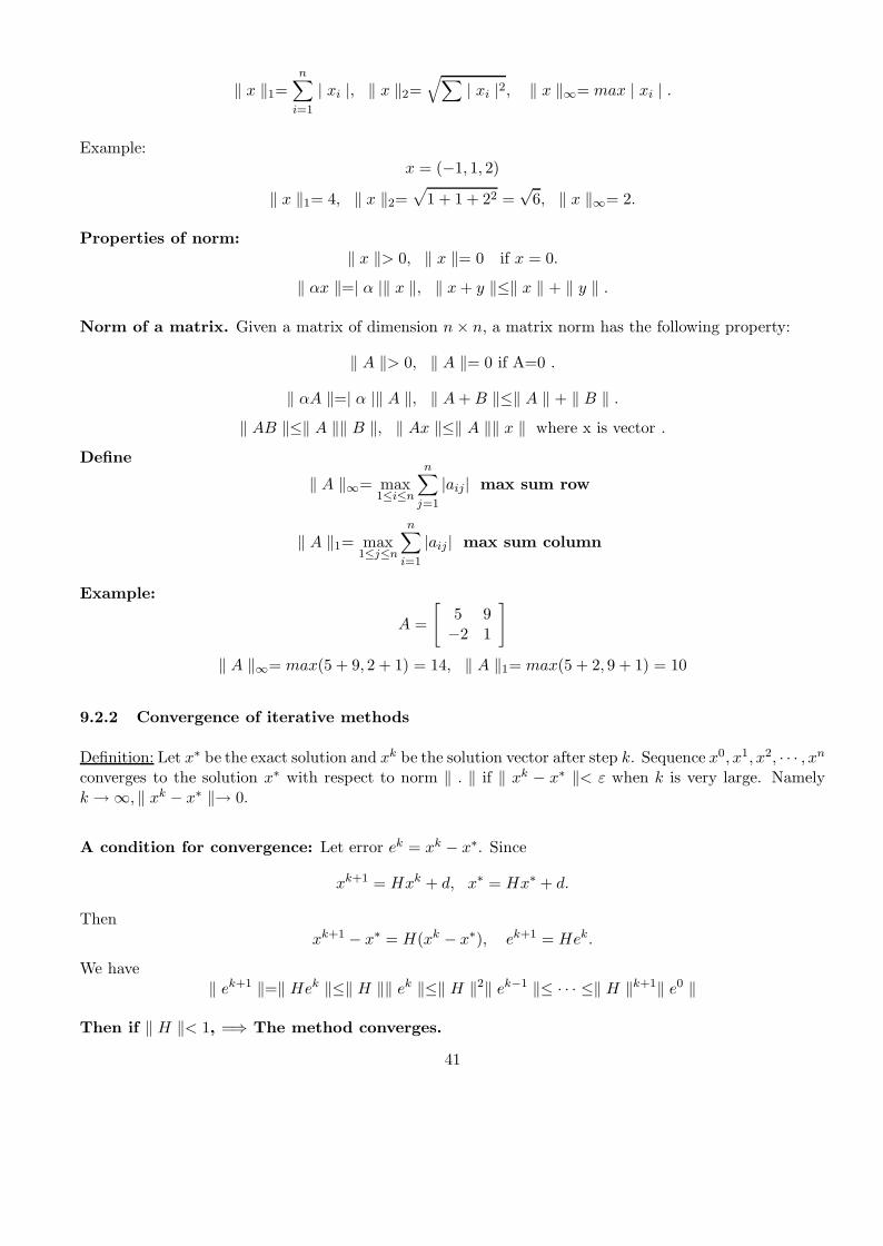
‖ x ‖1=n∑

i=1

| xi |, ‖ x ‖2=√∑

| xi |2, ‖ x ‖∞= max | xi | .

Example:x = (−1, 1, 2)

‖ x ‖1= 4, ‖ x ‖2=√

1 + 1 + 22 =√

6, ‖ x ‖∞= 2.

Properties of norm:‖ x ‖> 0, ‖ x ‖= 0 if x = 0.

‖ αx ‖=| α |‖ x ‖, ‖ x + y ‖≤‖ x ‖ + ‖ y ‖ .

Norm of a matrix. Given a matrix of dimension n × n, a matrix norm has the following property:

‖ A ‖> 0, ‖ A ‖= 0 if A=0 .

‖ αA ‖=| α |‖ A ‖, ‖ A + B ‖≤‖ A ‖ + ‖ B ‖ .

‖ AB ‖≤‖ A ‖‖ B ‖, ‖ Ax ‖≤‖ A ‖‖ x ‖ where x is vector .

Define

‖ A ‖∞= max1≤i≤n

n∑j=1

|aij| max sum row

‖ A ‖1= max1≤j≤n

n∑i=1

|aij | max sum column

Example:

A =

[5 9−2 1

]

‖ A ‖∞= max(5 + 9, 2 + 1) = 14, ‖ A ‖1= max(5 + 2, 9 + 1) = 10

9.2.2 Convergence of iterative methods

Definition: Let x∗ be the exact solution and xk be the solution vector after step k. Sequence x0, x1, x2, · · · , xn

converges to the solution x∗ with respect to norm ‖ . ‖ if ‖ xk − x∗ ‖< ε when k is very large. Namelyk → ∞, ‖ xk − x∗ ‖→ 0.

A condition for convergence: Let error ek = xk − x∗. Since

xk+1 = Hxk + d, x∗ = Hx∗ + d.

Thenxk+1 − x∗ = H(xk − x∗), ek+1 = Hek.

We have‖ ek+1 ‖=‖ Hek ‖≤‖ H ‖‖ ek ‖≤‖ H ‖2‖ ek−1 ‖≤ · · · ≤‖ H ‖k+1‖ e0 ‖

Then if ‖ H ‖< 1, =⇒ The method converges.

41

9.3 Jacobi Method for Ax = b

For each iteration:xk+1

i =1aii

(bi −∑j>i

aijxkj ) i = 1, · · · n

Example:(1) 6x1 − 2x2 + x3 = 11(2) −2x1 + 7x2 + 2x3 = 5(3) x1 + 2x2 − 5x3 = -1

=⇒x

(k+1)1 = 1

6(11 − (−2x(k)2 + x

(k)3 ))

x(k+1)2 = 1

7(5 − (−2x(k)1 + 2x(k)

3 ))x

(k+1)3 = 1

−5(−1 − (x(k)1 + 2x(k)

2 ))

Jacobi method in a matrix-vector form

⎛⎜⎝ x1

x2

x3

⎞⎟⎠

k+1

=

⎡⎢⎣ 0 2

6 −16

27 0 −2

715

25 0

⎤⎥⎦⎛⎜⎝ x1

x2

x3

⎞⎟⎠

k

+

⎛⎜⎝

1165715

⎞⎟⎠

In general:

A =

⎛⎜⎜⎜⎜⎝

a11 a12 · · · a1n

a21 a22 · · · a2n...

.... . .

...an1 an2 · · · ann

⎞⎟⎟⎟⎟⎠ , D =

⎛⎜⎜⎜⎜⎝

a11

a22

. . .ann

⎞⎟⎟⎟⎟⎠ , B = A − D.

Then from Ax = b,(D + B)x = b.

Thus Dx = −Bx + b, thenxk+1 = −D−1Bxk + D−1b

i.e.H = −D−1B, d = D−1b.

9.4 Parallel Jacobi Method

xk+1 = −D−1Bxk + D−1b

Parallel implementation:

• Distribute rows of B and the diagonal elements of D to processors.

• Perform computation based on the owner-computes rule.

• Perform all-all broadcasting after each iteration.

Note: If the iterative matrix is very sparse, i.e. containing a lot of zeros, the code design should takeadvantage of this and should not store those nonzeros. Also the code design should explicitly skip thoseoperations applied to zero elements.

42

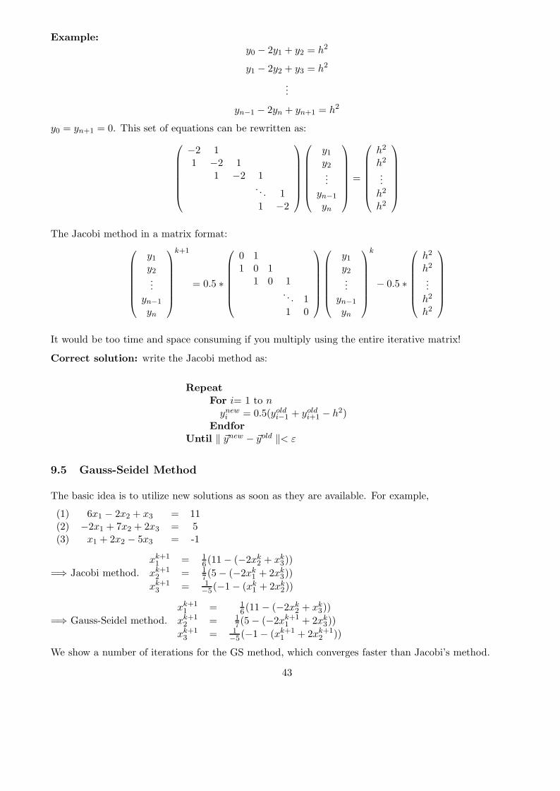
Example:y0 − 2y1 + y2 = h2

y1 − 2y2 + y3 = h2

...

yn−1 − 2yn + yn+1 = h2

y0 = yn+1 = 0. This set of equations can be rewritten as:⎛⎜⎜⎜⎜⎜⎜⎝

−2 11 −2 1

1 −2 1. . . 11 −2

⎞⎟⎟⎟⎟⎟⎟⎠

⎛⎜⎜⎜⎜⎜⎜⎝

y1

y2...

yn−1

yn

⎞⎟⎟⎟⎟⎟⎟⎠

=

⎛⎜⎜⎜⎜⎜⎜⎝

h2

h2

...h2

h2

⎞⎟⎟⎟⎟⎟⎟⎠

The Jacobi method in a matrix format:⎛⎜⎜⎜⎜⎜⎜⎝

y1

y2...

yn−1

yn

⎞⎟⎟⎟⎟⎟⎟⎠

k+1

= 0.5 ∗

⎛⎜⎜⎜⎜⎜⎜⎝

0 11 0 1

1 0 1. . . 11 0

⎞⎟⎟⎟⎟⎟⎟⎠

⎛⎜⎜⎜⎜⎜⎜⎝

y1

y2...

yn−1

yn

⎞⎟⎟⎟⎟⎟⎟⎠

k

− 0.5 ∗

⎛⎜⎜⎜⎜⎜⎜⎝

h2

h2

...h2

h2

⎞⎟⎟⎟⎟⎟⎟⎠

It would be too time and space consuming if you multiply using the entire iterative matrix!

Correct solution: write the Jacobi method as:

RepeatFor i= 1 to n

ynewi = 0.5(yold

i−1 + yoldi+1 − h2)

EndforUntil ‖ �ynew − �yold ‖< ε

9.5 Gauss-Seidel Method

The basic idea is to utilize new solutions as soon as they are available. For example,

(1) 6x1 − 2x2 + x3 = 11(2) −2x1 + 7x2 + 2x3 = 5(3) x1 + 2x2 − 5x3 = -1

=⇒ Jacobi method.xk+1

1 = 16 (11 − (−2xk

2 + xk3))

xk+12 = 1

7 (5 − (−2xk1 + 2xk

3))xk+1

3 = 1−5(−1 − (xk

1 + 2xk2))

=⇒ Gauss-Seidel method.xk+1

1 = 16 (11 − (−2xk

2 + xk3))

xk+12 = 1

7(5 − (−2xk+11 + 2xk

3))xk+1

3 = 1−5 (−1 − (xk+1

1 + 2xk+12 ))

We show a number of iterations for the GS method, which converges faster than Jacobi’s method.

43

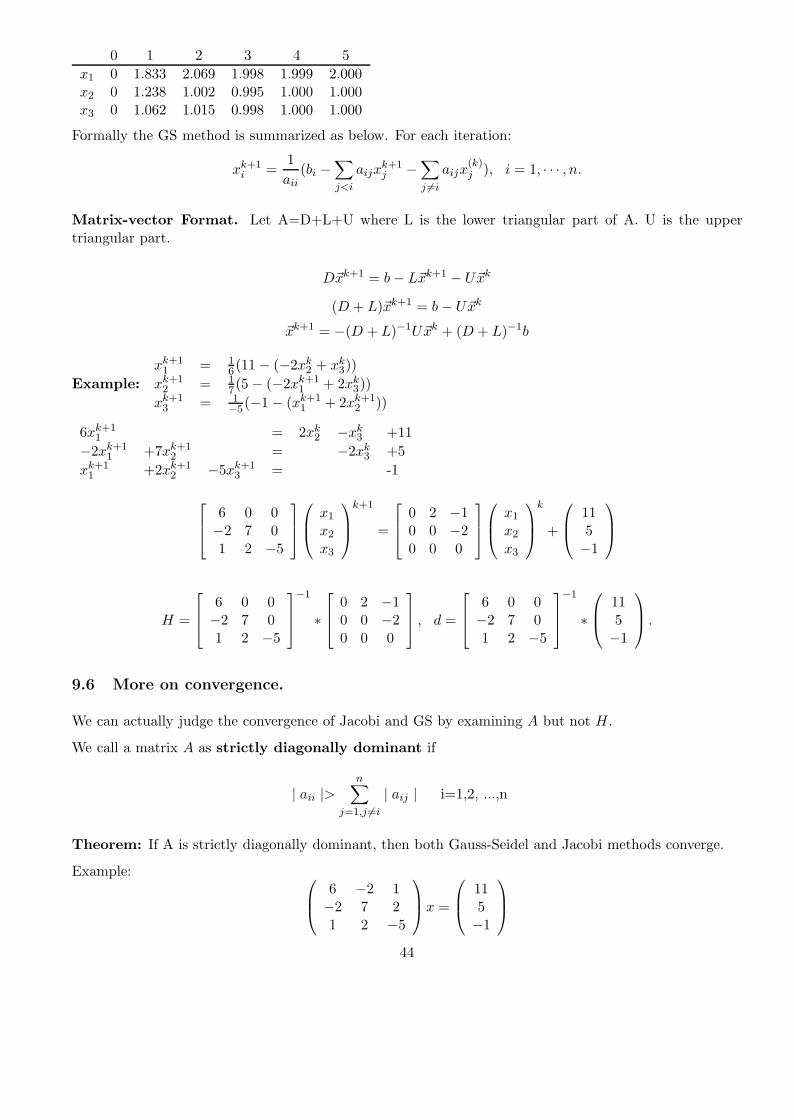
0 1 2 3 4 5x1 0 1.833 2.069 1.998 1.999 2.000x2 0 1.238 1.002 0.995 1.000 1.000x3 0 1.062 1.015 0.998 1.000 1.000

Formally the GS method is summarized as below. For each iteration:

xk+1i =

1aii

(bi −∑j<i

aijxk+1j −

∑j �=i

aijx(k)j ), i = 1, · · · , n.

Matrix-vector Format. Let A=D+L+U where L is the lower triangular part of A. U is the uppertriangular part.

D�xk+1 = b − L�xk+1 − U�xk

(D + L)�xk+1 = b − U�xk

�xk+1 = −(D + L)−1U�xk + (D + L)−1b

Example:xk+1

1 = 16(11 − (−2xk

2 + xk3))

xk+12 = 1

7(5 − (−2xk+11 + 2xk

3))xk+1

3 = 1−5(−1 − (xk+1

1 + 2xk+12 ))

6xk+11 = 2xk

2 −xk3 +11

−2xk+11 +7xk+1

2 = −2xk3 +5

xk+11 +2xk+1

2 −5xk+13 = -1

⎡⎢⎣ 6 0 0

−2 7 01 2 −5

⎤⎥⎦⎛⎜⎝ x1

x2

x3

⎞⎟⎠

k+1

=

⎡⎢⎣ 0 2 −1

0 0 −20 0 0

⎤⎥⎦⎛⎜⎝ x1

x2

x3

⎞⎟⎠

k

+

⎛⎜⎝ 11

5−1

⎞⎟⎠

H =

⎡⎢⎣ 6 0 0

−2 7 01 2 −5

⎤⎥⎦−1

∗⎡⎢⎣ 0 2 −1

0 0 −20 0 0

⎤⎥⎦ , d =

⎡⎢⎣ 6 0 0

−2 7 01 2 −5

⎤⎥⎦−1

∗⎛⎜⎝ 11

5−1

⎞⎟⎠ .

9.6 More on convergence.

We can actually judge the convergence of Jacobi and GS by examining A but not H.

We call a matrix A as strictly diagonally dominant if

| aii |>n∑

j=1,j �=i

| aij | i=1,2, ...,n

Theorem: If A is strictly diagonally dominant, then both Gauss-Seidel and Jacobi methods converge.

Example: ⎛⎜⎝ 6 −2 1

−2 7 21 2 −5

⎞⎟⎠x =

⎛⎜⎝ 11

5−1

⎞⎟⎠

44

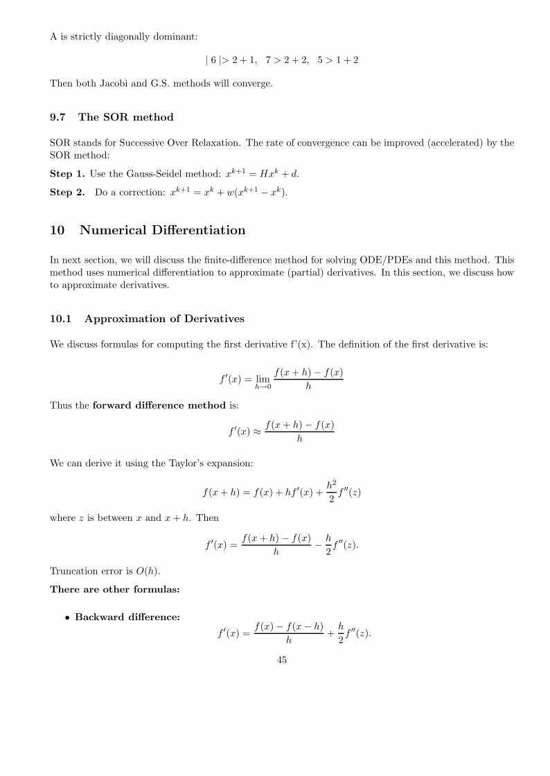
A is strictly diagonally dominant:

| 6 |> 2 + 1, 7 > 2 + 2, 5 > 1 + 2

Then both Jacobi and G.S. methods will converge.

9.7 The SOR method

SOR stands for Successive Over Relaxation. The rate of convergence can be improved (accelerated) by theSOR method:

Step 1. Use the Gauss-Seidel method: xk+1 = Hxk + d.

Step 2. Do a correction: xk+1 = xk + w(xk+1 − xk).

10 Numerical Differentiation

In next section, we will discuss the finite-difference method for solving ODE/PDEs and this method. Thismethod uses numerical differentiation to approximate (partial) derivatives. In this section, we discuss howto approximate derivatives.

10.1 Approximation of Derivatives

We discuss formulas for computing the first derivative f’(x). The definition of the first derivative is:

f ′(x) = limh→0

f(x + h) − f(x)h

Thus the forward difference method is:

f ′(x) ≈ f(x + h) − f(x)h

We can derive it using the Taylor’s expansion:

f(x + h) = f(x) + hf ′(x) +h2

2f ′′(z)

where z is between x and x + h. Then

f ′(x) =f(x + h) − f(x)

h− h

2f ′′(z).

Truncation error is O(h).

There are other formulas:

• Backward difference:

f ′(x) =f(x) − f(x − h)

h+

h

2f ′′(z).

45

• Central difference:

f(x + h) = f(x) − hf ′(x) +h2

2f ′′(x) +

h3

6f (3)(z1),

f(x − h) = f(x) − hf ′(x) +h2

2f ′′(x) − h3

6f (3)(z2).

Then

f(x + h) − f(x − h) = 2hf ′(x) +h3

6(f (3)(z1) − f (3)(z2)).

Thus the method is:

f(x) =f(x + h) − f(x − h)

2h+ O(

h2

3!).

10.2 Central difference for second-derivatives

f(x + h) = f(x) + hf ′(x) +h2

2f ′′(x) +

h3

3!f (3)(x) +

h4

4!f (4)(z1)

f(x − h) = f(x) − hf ′(x) +h2

2f ′′(x) − h3

3!f (3)(x) +

h4

4!f (4)(z2)

f(x + h) + f(x − h) = 2f(x) + h2f ′′(z) + O(h4

4!).

Thus:

f ′′(x) =f(x + h) + f(x − h) − 2f(x)

h2+ O(

h2

4!).

10.3 Example

We approximate f ′(x) = (cos x)′ at x = π6 using the forward difference formula.

i h f(x+h)−f(x)h Error Ei

Ei−1

Ei

1 0.1 -0.54243 0.042432 0.05 -0.52144 0.02144 1.983 0.025 -0.51077 0.01077 1.99

From this case, we can see that this truncation error Ei is proportional to h. If h is halved, =⇒, the erroris also halved.

We approximate f ′′(x) = (cos x)′′ at x = π6 . Using the central difference formula f ′′(x) ≈ (f(x + h) −

2f(x) + f(x − h))/h2, we have:

i h f ′′(x) ≈ Error EiEi−1

Ei

1 0.5 -0.84813289 0.01789292 0.25 -0.86152424 0.04504 3.973 0.125 -0.86489835 0.0127 3.994 0.0625 -0.86574353 0.002819 4.00

The truncation error Ei is proportional to h2.

46

11 ODE and PDE

ODE stands for Ordinary Differential Equations. PDE stands for Partial Differential Equations.

An ODE Example: Growth of Population

• Population : N(t), t is time.

• Assumption : Population in a state grows continuously with time at a birth rate (λ) proportionalto the number of persons. Let δ be the average number of persons moving-in to this state (aftersubtracting the moving-out number.)

d N(t)dt

= λN(t) + δ.

• Let λ = 0.01. δ = 0.045 million.

d N(t)dt

= 0.01N(t) + 0.045.

• If N(1990) = 1million, what are N(1991), N(1992), N(1993), · · · , N(1999)?

Other Examples

•

f ′(x) = x f(0) = 0.

What are f(0.1), f(0.2), · · · , f(0.5)?•

f”(x) = 1, f(0) = 1, f(1) = 1.5.

What are f(0.2), f(0.4), f(0.6), f(0.8)?

• The Laplace PDE.∂2U(x, y)

∂x2+

∂2U(x, y)∂y2

= 0.

The domain is a 2D region. Usually we know some boundary values or condition and we need to findvalues for some points within this region.

11.1 Finite Difference Method

1. Discretize a region or interval of variables, or domain of this function.

2. For each point in the discretized domain, setup an equation using a numerical differentiation formula.

3. Solve the linear equations.

47

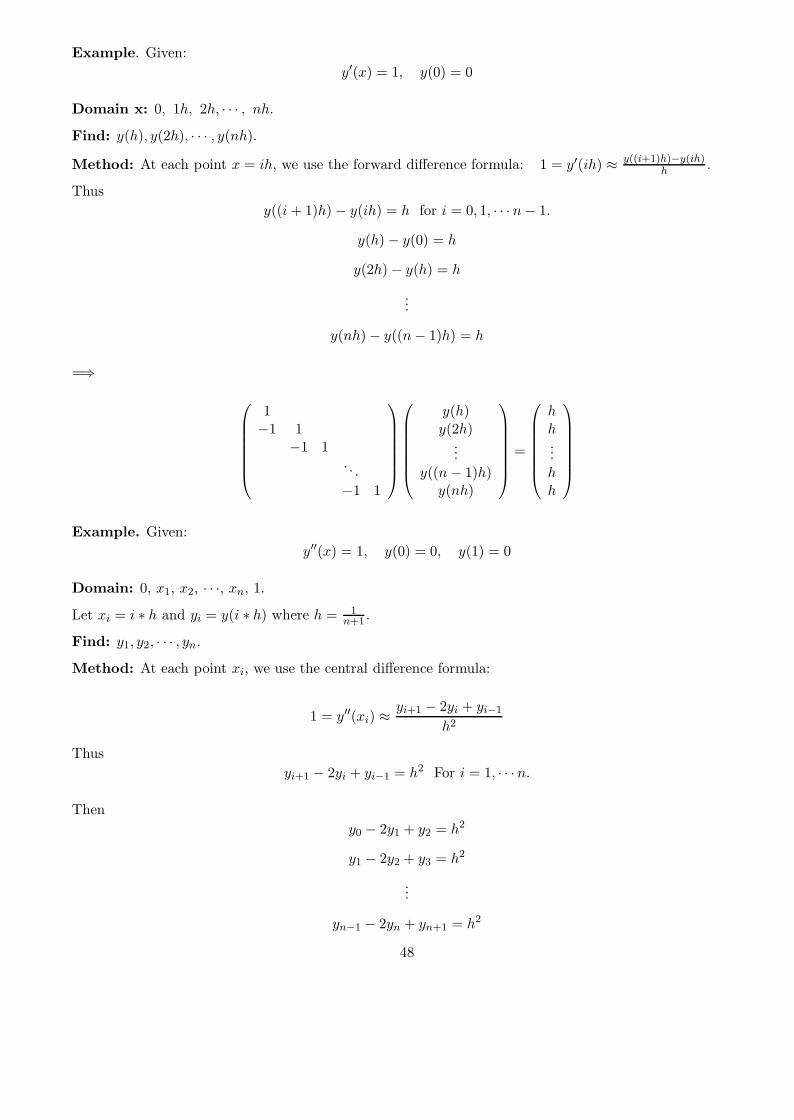
Example. Given:y′(x) = 1, y(0) = 0

Domain x: 0, 1h, 2h, · · · , nh.

Find: y(h), y(2h), · · · , y(nh).

Method: At each point x = ih, we use the forward difference formula: 1 = y′(ih) ≈ y((i+1)h)−y(ih)h .

Thusy((i + 1)h) − y(ih) = h for i = 0, 1, · · · n − 1.

y(h) − y(0) = h

y(2h) − y(h) = h

...

y(nh) − y((n − 1)h) = h

=⇒⎛⎜⎜⎜⎜⎜⎜⎝

1−1 1

−1 1. . .−1 1

⎞⎟⎟⎟⎟⎟⎟⎠

⎛⎜⎜⎜⎜⎜⎜⎝

y(h)y(2h)

...y((n − 1)h)

y(nh)

⎞⎟⎟⎟⎟⎟⎟⎠

=

⎛⎜⎜⎜⎜⎜⎜⎝

hh...hh

⎞⎟⎟⎟⎟⎟⎟⎠

Example. Given:y′′(x) = 1, y(0) = 0, y(1) = 0

Domain: 0, x1, x2, · · ·, xn, 1.

Let xi = i ∗ h and yi = y(i ∗ h) where h = 1n+1 .

Find: y1, y2, · · · , yn.

Method: At each point xi, we use the central difference formula:

1 = y′′(xi) ≈ yi+1 − 2yi + yi−1

h2

Thusyi+1 − 2yi + yi−1 = h2 For i = 1, · · · n.

Theny0 − 2y1 + y2 = h2

y1 − 2y2 + y3 = h2

...

yn−1 − 2yn + yn+1 = h2

48

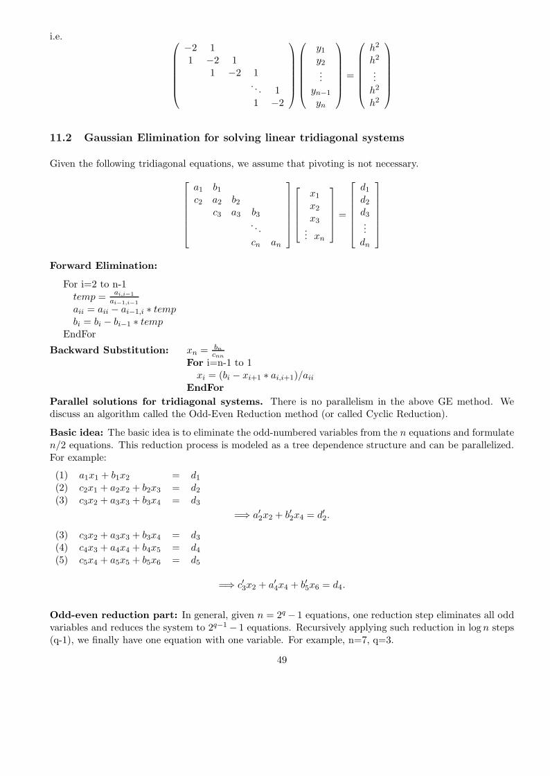
i.e. ⎛⎜⎜⎜⎜⎜⎜⎝

−2 11 −2 1

1 −2 1. . . 11 −2

⎞⎟⎟⎟⎟⎟⎟⎠

⎛⎜⎜⎜⎜⎜⎜⎝

y1

y2...

yn−1

yn

⎞⎟⎟⎟⎟⎟⎟⎠

=

⎛⎜⎜⎜⎜⎜⎜⎝

h2

h2

...h2

h2

⎞⎟⎟⎟⎟⎟⎟⎠

11.2 Gaussian Elimination for solving linear tridiagonal systems

Given the following tridiagonal equations, we assume that pivoting is not necessary.

⎡⎢⎢⎢⎢⎢⎢⎣

a1 b1

c2 a2 b2

c3 a3 b3

. . .cn an

⎤⎥⎥⎥⎥⎥⎥⎦

⎡⎢⎢⎢⎢⎣

x1

x2

x3... xn

⎤⎥⎥⎥⎥⎦ =

⎡⎢⎢⎢⎢⎢⎢⎣

d1

d2

d3...

dn

⎤⎥⎥⎥⎥⎥⎥⎦

Forward Elimination:

For i=2 to n-1temp = ai,i−1

ai−1,i−1

aii = aii − ai−1,i ∗ tempbi = bi − bi−1 ∗ temp

EndFor

Backward Substitution: xn = bncnn

For i=n-1 to 1xi = (bi − xi+1 ∗ ai,i+1)/aii

EndForParallel solutions for tridiagonal systems. There is no parallelism in the above GE method. Wediscuss an algorithm called the Odd-Even Reduction method (or called Cyclic Reduction).

Basic idea: The basic idea is to eliminate the odd-numbered variables from the n equations and formulaten/2 equations. This reduction process is modeled as a tree dependence structure and can be parallelized.For example:

(1) a1x1 + b1x2 = d1

(2) c2x1 + a2x2 + b2x3 = d2

(3) c3x2 + a3x3 + b3x4 = d3

=⇒ a′2x2 + b′2x4 = d′2.

(3) c3x2 + a3x3 + b3x4 = d3

(4) c4x3 + a4x4 + b4x5 = d4

(5) c5x4 + a5x5 + b5x6 = d5

=⇒ c′3x2 + a′4x4 + b′5x6 = d4.

Odd-even reduction part: In general, given n = 2q − 1 equations, one reduction step eliminates all oddvariables and reduces the system to 2q−1 − 1 equations. Recursively applying such reduction in log n steps(q-1), we finally have one equation with one variable. For example, n=7, q=3.

49

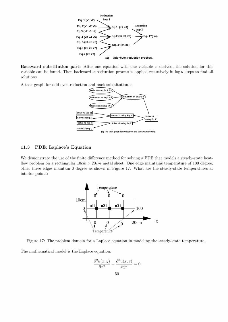
Eq. 1 (x1 x2)

Eq. 2(x1 x2 x3)

Eq.3 (x2 x3 x4)

Eq. 4 (x3 x4 x5)

Eq. 5 (x4 x5 x6)

Eq.6 (x5 x6 x7)

Eq.7 (x6 x7)

Eq.1’ (x2 x4)

Eq. 3’ (x4 x6)

Eq. 1’’( x4)

(a) Odd−even reduction process.

ReductionStep 1

Reductionstep 2

Eq.2’(x2 x4 x6)

Backward substitution part: After one equation with one variable is derived, the solution for thisvariable can be found. Then backward substitution process is applied recursively in log n steps to find allsolutions.

A task graph for odd-even reduction and back substitution is:Reduction on Eq 1 2 3

Reduction on Eq 3 4 5

Reduction on Eq 5 6 7

Reduction on Eq 1’2’3’

Solve x1 (Eq 1)

Solve x5 (Eq 5)

Solve x3 (Eq 3)

Solve x7 (Eq 7)

using Eq. 1’Solve x2

Solve x6 using Eq 3’

Solve x4using Eq 1’’

(b) The task graph for reduction and backward solving.

11.3 PDE: Laplace’s Equation

We demonstrate the use of the finite difference method for solving a PDE that models a steady-state heat-flow problem on a rectangular 10cm × 20cm metal sheet. One edge maintains temperature of 100 degree,other three edges maintain 0 degree as shown in Figure 17. What are the steady-state temperatures atinterior points?

0

0 0

0 0 0

100

0

Temperature

x

Temperature

10cm

20cm

u11 u21 u31

Figure 17: The problem domain for a Laplace equation in modeling the steady-state temperature.

The mathematical model is the Laplace equation:

∂2u(x, y)∂x2

+∂2u(x, y)

∂y2= 0

50

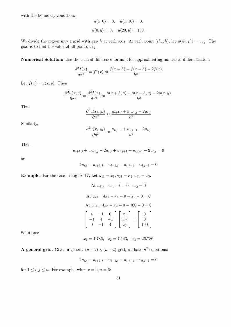
with the boundary condition:u(x, 0) = 0, u(x, 10) = 0.

u(0, y) = 0, u(20, y) = 100.

We divide the region into a grid with gap h at each axis. At each point (ih, jh), let u(ih, jh) = ui,j. Thegoal is to find the value of all points ui,j.

Numerical Solution: Use the central difference formula for approximating numerical differentiation:

d2f(x)dx2

= f ′′(x) ≈ f(x + h) + f(x − h) − 2f(x)h2

Let f(x) = u(x, y). Then

∂2u(x, y)∂x2

=d2f(x)

dx2≈ u(x + h, y) + u(x − h, y) − 2u(x, y)

h2.

Thus∂2u(xi, yi)

∂x2≈ ui+1,j + ui−1,j − 2ui,j

h2

Similarly,∂2u(xi, yi)

∂y2≈ ui,j+1 + ui,j−1 − 2ui,j

h2

Thenui+1,j + ui−1,j − 2ui,j + ui,j+1 + ui,j−1 − 2ui,j = 0

or4ui,j − ui+1,j − ui−1,j − ui,j+1 − ui,j−1 = 0

Example. For the case in Figure 17, Let u11 = x1, u21 = x2, u31 = x3.

At u11, 4x1 − 0 − 0 − x2 = 0

At u21, 4x2 − x1 − 0 − x3 − 0 = 0

At u31, 4x3 − x2 − 0 − 100 − 0 = 0⎡⎢⎣ 4 −1 0

−1 4 −10 −1 4

⎤⎥⎦⎡⎢⎣ x1

x2

x3

⎤⎥⎦ =

⎡⎢⎣ 0

0100

⎤⎥⎦

Solutions:x1 = 1.786, x2 = 7.143, x3 = 26.786

A general grid. Given a general (n + 2) × (n + 2) grid, we have n2 equations:

4ui,j − ui+1,j − ui−1,j − ui,j+1 − ui,j−1 = 0

for 1 ≤ i, j ≤ n. For example, when r = 2, n = 6:

51

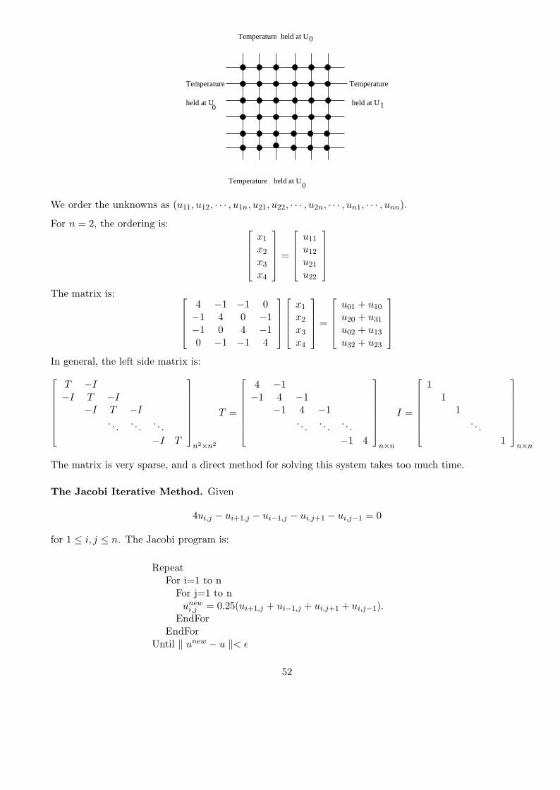
Temperature

held at U0

Temperature

held at U1

held at U

Temperature held at U

Temperature

0

0

We order the unknowns as (u11, u12, · · · , u1n, u21, u22, · · · , u2n, · · · , un1, · · · , unn).

For n = 2, the ordering is: ⎡⎢⎢⎢⎣

x1

x2

x3

x4

⎤⎥⎥⎥⎦ =

⎡⎢⎢⎢⎣

u11

u12

u21

u22

⎤⎥⎥⎥⎦

The matrix is: ⎡⎢⎢⎢⎣

4 −1 −1 0−1 4 0 −1−1 0 4 −10 −1 −1 4

⎤⎥⎥⎥⎦⎡⎢⎢⎢⎣

x1

x2

x3

x4

⎤⎥⎥⎥⎦ =

⎡⎢⎢⎢⎣

u01 + u10

u20 + u31

u02 + u13

u32 + u23

⎤⎥⎥⎥⎦

In general, the left side matrix is:⎡⎢⎢⎢⎢⎢⎢⎣

T −I−I T −I

−I T −I. . . . . . . . .

−I T

⎤⎥⎥⎥⎥⎥⎥⎦

n2×n2

T =

⎡⎢⎢⎢⎢⎢⎢⎣

4 −1−1 4 −1

−1 4 −1. . . . . . . . .

−1 4

⎤⎥⎥⎥⎥⎥⎥⎦

n×n

I =

⎡⎢⎢⎢⎢⎢⎢⎣

11

1. . .

1

⎤⎥⎥⎥⎥⎥⎥⎦

n×n

The matrix is very sparse, and a direct method for solving this system takes too much time.

The Jacobi Iterative Method. Given

4ui,j − ui+1,j − ui−1,j − ui,j+1 − ui,j−1 = 0

for 1 ≤ i, j ≤ n. The Jacobi program is:

RepeatFor i=1 to n

For j=1 to nunew

i,j = 0.25(ui+1,j + ui−1,j + ui,j+1 + ui,j−1).EndFor

EndForUntil ‖ unew − u ‖< ε

52

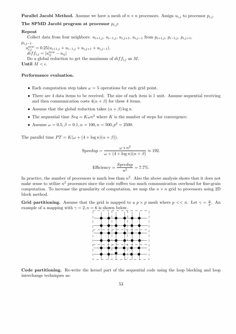
Parallel Jacobi Method. Assume we have a mesh of n × n processors. Assign ui,j to processor pi,j.

The SPMD Jacobi program at processor pi,j:

RepeatCollect data from four neighbors: ui+1,j, ui−1,j , ui,j+1, ui,j−1 from pi+1,j, pi−1,j, pi,j+1,

pi,j−1.unew

i,j = 0.25(ui+1,j + ui−1,j + ui,j+1 + ui,j−1).diffi,j = |unew

ij − uij|Do a global reduction to get the maximum of diffi,j as M .

Until M < ε.

Performance evaluation.

• Each computation step takes ω = 5 operations for each grid point.

• There are 4 data items to be received. The size of each item is 1 unit. Assume sequential receivingand then communication costs 4(α + β) for these 4 items.

• Assume that the global reduction takes (α + β) log n.

• The sequential time Seq = Kωn2 where K is the number of steps for convergence.

• Assume ω = 0.5, β = 0.1, α = 100, n = 500, p2 = 2500.

The parallel time PT = K(ω + (4 + log n)(α + β)).

Speedup =ω ∗ n2

ω + (4 + log n)(α + β)≈ 192.

Efficiency =Speedup

n2= 7.7%.

In practice, the number of processors is much less than n2. Also the above analysis shows that it does notmake sense to utilize n2 processors since the code suffers too much communication overhead for fine-graincomputation. To increase the granularity of computation, we map the n × n grid to processors using 2Dblock method.

Grid partitioning. Assume that the grid is mapped to a p × p mesh where p << n. Let γ = np . An

example of a mapping with γ = 2, n = 6 is shown below.

Code partitioning. Re-write the kernel part of the sequential code using the loop blocking and loopinterchange techniques as:

53

For bi = 1 to pFor bj = 1 to pFor i = (bi − 1)γ + 1 to biγFor j = (bj − 1)γ + 1 to bjγunew


EndForEndFor

EndFor

Parallel SPMD code. On processor pbi,bj:

RepeatCollect the data from its four neighbors.For i = (bi − 1)γ + 1 to biγFor j = (bj − 1)γ + 1 to bjγunew


EndForCompute the local maximum diffbi,bj

for the difference between old values and newvalues.

Do a global reduction to get the maximum diffbi,bjas M .

Until M < ε.

Performance evaluation.

• At each processor, each computation step takes ωω2 operations.

• The communication cost for each step on each processor is 4(α + ωβ).

• Assume that the global reduction takes (α + β) log p.

• The number of steps for convergence is K.

• Assume ω = 0.5, β = 0.1, α = 100, n = 500, ω = 100, p2 = 25.

PT = K(ω2ω + (4 + log p)(α + rβ))

Speedup =ωω2p2

ω2ω + (4 + log p)(α + ωβ)≈ 21.2.

Efficiency = 84%.

Red-Black Ordering. Reordering variables can eliminate most of data dependence in the Gauss Seidelalgorithm for this PDE problem.

54

��

��

��

��

��

��

��

��

��

��

��

��

��

��

��

��

��

��

��

��

��

��

��

��

��

��

��

��

��

��

��

��

��

��

��

��

• Points are divided into “red” points (white) and black points.

• First, black points are computed (using the old red point values).

• Second, red points are computed (using the new black point values).

Parallel code for red-black ordering

• Point (i,j) is black if i+j is even.

• Point (i,j) is red if i+j is odd.

• Computation on black points (stage 1) can be done in parallel.

• Computation on red points (stage 2) can be done in parallel.

The Kernel code:

• For all points (i,j) with (i+j) mod 2=0, do in parallel

ui,j = 0.25(ui+1,j + ui−1,j + ui,j+1 + ui,j−1).

• For all points (i,j) with (i+j) mod 2=1, do in parallel

ui,j = 0.25(ui+1,j + ui−1,j + ui,j+1 + ui,j−1).

A MPI Parallel Programming

References: 1) MPI standard (HTML): www.mcs.anl.gov/mpi/mpi-report-1.1/mpi-report.html. 2) MPItutorial (PS file) is available at the CS110B homepage. 3) On-line MPI book (HTML): www.netlib.org/utk/papers/mbook/mpi-book.html.

MPI is to establish a widely used language- and platform-independent standard for writing message-passingprograms. Six MPI basic library functions are:

• MPI Init(). – Initiate an MPI computation.

• MPI Finalize(). – Terminate a computation.

• MPI Comm size() – Determine number of processes.

55

• MPI Comm rank()– Determine my process identifier.

• MPI Send() – Send a message.

• MPI Recv() – Receive a message.

For MPI programming, the concept “process” is about the same as “processor” (in this course). Com-municator indicates the process group in which communication occurs. We use MPI COMM WORLD forthis course.

Example: hello.c

#include <stdio.h>#include "mpi.h"main(int argc, char* argv[]) {

int my_rank;MPI_Init(&argc, &argv);MPI_Comm_rank(MPI_COMM_WORLD, &my_rank);printf("Hello from node %d\n", my_rank);MPI_Finalize();/* Shut down MPI */

}

The result:

Hello from node 3Hello from node 1Hello from node 2Hello from node 0

Basic functions:

• Blocking send

int MPI_Send(void* buf, int count, MPI_Datatype datatype, int dest, int tag, MPI_Comm comm

– buf — initial address of send buffer

– count — number of elements in send buffer (nonnegative integer)

– datatype — datatype of each send buffer element

– dest — rank of destination

– tag — message tag

– comm — communicator

It does not return until the message has been safely stored away so that the sender is free to overwritethe send buffer. The message might be copied directly into the matching receive buffer, or it mightbe copied into a temporary system buffer.

• Blocking receive

int MPI_Recv(void* buf, int count, MPI_Datatype datatype, int source, int tag,MPI_Comm comm, MPI_Status *status)

56

– buf — initial address of receive buffer

– count — number of elements in receive buffer

– datatype — datatype of each receive buffer element

– source — rank of source

– tag — message tag

– comm — communicator

– status — the status of this communication.

The wildcards MPI ANY SOURCE and MPI ANY TAG indicate that any source and/or tag areacceptable.

• MPI datatype: MPI CHAR. MPI SHORT. MPI INT. MPI LONG. MPI FLOAT. MPI DOUBLE.

• Actions of MPI Send()

Network

Send Receive

User data

SystemBuffer

SystemBuffer

User space

Proc 0: MPI Send(&data[0],100, MPI CHAR,1, 1,MPI COMM WORLD).

– Retrieve data[0] data[1] ... data[100].

– Copy this msg with name=1 to the local system buffer or directly deliver/copy to a buffer atprocessor 1.

• Actions of MPI Recv()

Proc 1: MPI Recv( &data[0], 100, MPI CHAR,0,1,MPI COMM WORLD, &status).

– Wait until a message from processor 0 with name=1 arrives at the local buffer.

– Then copy the msg to data[0], data[1],... .

Proc 1: MPI Recv( &data[0], 100, MPI CHAR,MPI ANY SOURCE, MPI ANY TAG,MPI CO&status)

– Wait until any msg arrives at the buffer.

– Copy the msg to data[0], data[1],....

Example (greetings.c): Send a message from all processes with rank �= 0 to process 0. Process 0 printsthe messages received.

57

#include <stdio.h>#include <string.h>#include "mpi.h"

main(int argc, char* argv[]){int my_rank; /*rank of process */int p; /*number of processes*/int source; /*rank of sender */int dest; /*rank of receiver */int tag = 0; /*tag for messages */char message[100];/*storage for message*/MPI_Status status; /*return status for */

/*receive */MPI_Init(&argc, &argv);MPI_Comm_rank(MPI_COMM_WORLD, &my_rank);MPI_Comm_size(MPI_COMM_WORLD, &p);

if (my_rank != 0) {sprintf(message, "Greetings from process %d!",

my_rank);dest = 0;MPI_Send(message, strlen(message)+1, MPI_CHAR, dest, tag, MPI_COMM_WORLD);

}else {for (source = 1; source < p; source++) {

MPI_Recv(message, 100, MPI_CHAR, source, tag, MPI_COMM_WORLD, &status);printf("%s\n", message);

}}MPI_Finalize();

}

An example for numerical integration The trapezoidal rule:

∫ b

af(x)dx ≈ f(a) + f(b)

2(b − a)

If interval [a, b] is divided into n sub-intervals,

xi = a + i ∗ h for 0 ≤ i ≤ n, h =b − a

n.

∫ b

af(x)dx ≈

n−1∑i=0

f(xi) + f(xi+1)2

h = [f(a)/2 + f(b)/2 + f(x1) + f(x2) + · · · + f(xn−1)]h.

Sequential code

Trap(float a,float b, int n, float h ){integral = (f(a) + f(b))/2.0;x = a;for (i = 1; i <= n-1; i++) {

58

x = x + h;integral = integral + f(x);

}integral = integral*h;return(integral);

}

Parallel numerical integration:

• 1. Each process calculates “its” interval of integration.

• 2. Each process estimates the integral of f(x) over its interval.

• 3 Each process (�= 0) sends its integral to process 0.

• 4 Process 0 sums the calculations received from the individual processes and prints the result.

The MPI code

MPI_Comm_rank(MPI_COMM_WORLD, &my_rank);MPI_Comm_size(MPI_COMM_WORLD, &p);/* Local computation*/h = (b-a)/n;local_n = n/p;local_a = a + my_rank*local_n*h;local_b = local_a + local_n*h;integral = Trap(local_a, local_b, local_n, h);/*Add up the integrals from each process*/if (my_rank == 0) {total = integral;for (source = 1; source < p; source++) {

MPI_Recv(&integral, 1, MPI_FLOAT, source, tag, MPI_COMM_WORLD, &status);total = total + integral;

}} else {

MPI_Send(&integral, 1, MPI_FLOAT, dest, tag, MPI_COMM_WORLD);}

Other issues

• Parallel I/O issues: Given SPMD code:

scanf("%f %f %d", a_ptr, b_ptr, n_ptr);

We run this code on two nodes, and type “ 0 1 1024”. What happens? Many possibilities:

– Both processes get the data.

– One process gets the data.

– Process 0 gets “0 1” and Process 1 gets “1024”.

59

There is no consensus yet in parallel computing world. Solution: Have one process do I/O.

• I/O in the trapezoidal code:

– 1. Process 0 reads the input.

– 2. Process 0 sends input values to other processes.

if (my_rank == 0){printf("Enter a, b, and n\n");scanf("%f %f %d", &a, &b, &n);for (dest = 1; dest < p; dest++){tag = 0;MPI_Send(&a, 1, MPI_FLOAT, dest, tag, MPI_COMM_WORLD);tag = 1;MPI_Send(&b, 1, MPI_FLOAT, dest, tag, MPI_COMM_WORLD);tag = 2;MPI_Send(&n, 1, MPI_INT, dest, tag, MPI_COMM_WORLD);

}} else {

tag = 0;MPI_Recv(&a, 1, MPI_FLOAT, source, tag, MPI_COMM_WORLD, &status);tag = 1;MPI_Recv(&b, 1, MPI_FLOAT, source, tag, MPI_COMM_WORLD, &status);tag = 2;MPI_Recv(&n, 1, MPI_INT, source, tag, MPI_COMM_WORLD, &status);}

}

• Group data for communication: Can we send a, b, and n together in one message?

struct{float a_part;float b_part;int n_part;

} z;

z.a_part=a;z.b_part=b;z.n_part=n;if (my_rank == 0){

for (dest = 1; dest < p; dest++)MPI_Send(&z, sizeof(z), MPI_CHAR, dest, 0, MPI_COMM_WORLD);

}elseMPI_Recv(&z, sizeof(z), MPI_CHAR, source, 0, MPI_COMM_WORLD, &status);

Collective Communication: Global operations over a group of processes.

• MPI Barrier (comm) — Each process in the comm blocks until every process in comm has calledit.

60

• MPI Bcast (buffer, count, datatype, root, comm) — Broadcast from one member of the groupto all other members.

• MPI Reduce (operand, result, count, datatype, operator, root, comm) — Global reductionoperations such as max, min, sum, product, and min and max operations.

• MPI Gather (sendbuf, sendcount, sendtype, recvbuf, recvcount, recvtype, root, comm)— Gather data from all group members to one process.

• MPI Scatter(sendbuf, sendcount, sendtype, recvbuf, recvcount, recvtype, root, comm).— Scatter data from one group member to all other members.

An example of MPI Bcast(). In the trapezoidal code, Process 0 prompts user for input and reads inthe values. Then it broadcasts input values to other processes.

if (my_rank == 0) {printf("Enter a, b, and n\n");scanf("%f %f %d", &a, &b, &n);

}MPI_Bcast(&a, 1, MPI_FLOAT, 0, MPI_COMM_WORLD);MPI_Bcast(&b, 1, MPI_FLOAT, 0, MPI_COMM_WORLD);MPI_Bcast(&n, 1, MPI_INT, 0, MPI_COMM_WORLD);

An example of MPI Reduce In the trapezoidal code, use MPI Reduce to do global summation foradding up the integrals calculated by each process.

MPI_Reduce(&integral, &total, 1, MPI_FLOAT, MPI_SUM, 0, MPI_COMM_WORLD);

MPI Gather():

int MPI_Gather(void* sendbuf, int sendcount, MPI_Datatype sendtype, void* recvbuf,int recvcount, MPI_Datatype recvtype, int root, MPI_Comm comm)

• sendbuf – starting address of send buffer

• sendcount – number of elements in send buffer

• sendtype – data type of send buffer elements

• recvbuf – address of receive buffer (significant only at root)

• recvcount – number of elements for any single receive (significant only at root)

• recvtype – data type of recv buffer elements (significant only at root)

• root – rank of receiving process

• comm – communicator.

61

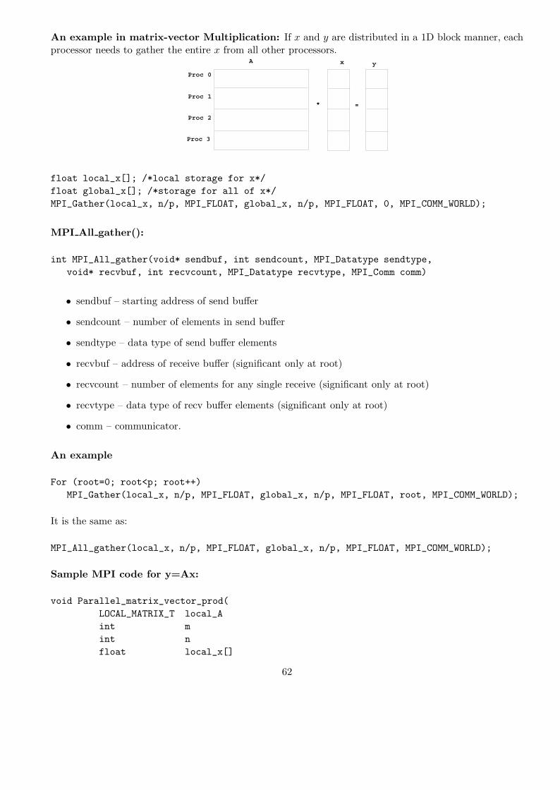
An example in matrix-vector Multiplication: If x and y are distributed in a 1D block manner, eachprocessor needs to gather the entire x from all other processors.

Proc 0

Proc 1

Proc 2

Proc 3

A x y

* =

float local_x[]; /*local storage for x*/float global_x[]; /*storage for all of x*/MPI_Gather(local_x, n/p, MPI_FLOAT, global_x, n/p, MPI_FLOAT, 0, MPI_COMM_WORLD);

MPI All gather():

int MPI_All_gather(void* sendbuf, int sendcount, MPI_Datatype sendtype,void* recvbuf, int recvcount, MPI_Datatype recvtype, MPI_Comm comm)

• sendbuf – starting address of send buffer

• sendcount – number of elements in send buffer

• sendtype – data type of send buffer elements

• recvbuf – address of receive buffer (significant only at root)

• recvcount – number of elements for any single receive (significant only at root)

• recvtype – data type of recv buffer elements (significant only at root)

• comm – communicator.

An example

For (root=0; root<p; root++)MPI_Gather(local_x, n/p, MPI_FLOAT, global_x, n/p, MPI_FLOAT, root, MPI_COMM_WORLD);

It is the same as:

MPI_All_gather(local_x, n/p, MPI_FLOAT, global_x, n/p, MPI_FLOAT, MPI_COMM_WORLD);

Sample MPI code for y=Ax:

void Parallel_matrix_vector_prod(LOCAL_MATRIX_T local_Aint mint nfloat local_x[]

62

float global_x[]float local_y[]int local_mint local_n) {

/* local_m = n/p, local_n = n/p */int i, j;MPI_Allgather(local_x, local_n, MPI_FLOAT, global_x, local_n, MPI_FLOAT, MPI_COMM_WORLD);for (i = 0; i < local_m; i++) {

local_y[i] = 0.0;for (j = 0; j < n; j++)local_y[i] = local_y[i] +

local_A[i][j]*global_x[j];}

}

B Pthreads

References: On-line material: www.cs.ucsb.edu/∼tyang/class/pthreads/.

B.1 Introduction

Ptheads can be used to exploit parallelism on shared memory multiprocessor machines and implement con-current processing on sequential machines. Conceptually, threads execute concurrently. This is the bestway to reason about the behavior of threads. But in practice, a machine may only have a finite number ofprocessors, and it can’t run all of the runnable threads at once. So, it must multiplex the runnable threadson the finite number of processors.

Pthreads is the POSIX 1003.1c thread standard put out by the IEEE standards committee. This standardgot approval from the international Standards Organization (ISO) Committee and the IEEE StandardsBoard in 1995. Currently Pthreads implementation is available in commercial UNIX platforms. The NTplatform supports another type of thread programming; however, its basic concept is similar to Pthreads.We discuss a number of basic pthread routines below. You can can get the detailed specification using theUnix man command.

Notice that you should put “#include <pthread.h>” at the beginning of your program file. In compilingthe code, you should put “-lpthread” in linking the code. The Web page of 110B provides sample pthreadcode and the makefile.

B.2 Thread creation and manipulation

• pthread create()

int pthread_create(pthread_t * thread, const pthread_attr_t * attr,void * (*start_routine)(void *), void * arg);

63

The pthread create() routine creates a new thread within a process. The new thread starts in thestart routine start routine which has a start argument arg. The new thread has attributes specifiedwith attr, or default attributes if attr is NULL.

If the pthread create() routine succeeds it will return 0 and put the new thread id into thread,otherwise an error number shall be returned indicating the error.

• pthread attr init()

int pthread_attr_init(pthread_attr_t *attr);

This routine creates and initializes an attribute variable (e.g. scheduling policy) for the use withpthread create(). If the pthread attr init() routine succeeds it will return 0 and put the new attributevariable id into attr, otherwise an error number shall be returned indicating the error.

• pthread equal()

int pthread_equal(pthread_t thread_1, pthread_t thread_2);

The pthread equal() routine compares the thread ids thread 1 and thread 2 and returns a non 0value if the ids represent the same thread otherwise 0 is returned.

• pthread exit()

void pthread_exit(void * status);

The pthread exit() routine terminates the currently running thread and makes status available tothe thread that successfully joins (pthread join()), with the terminating thread.

An implicit call to pthread exit() is made if any thread, other than the thread in which main() wasfirst called, returns from the start routine specified in pthread create(). The return value takes theplace of status.

The process exits as if exit() was called with a status of 0 if the terminating thread is the last threadin the process.

The pthread exit() routine cannot return.

• pthread join()

int pthread_join(pthread_t thread, void ** status);

If the target thread thread is not detached and there are no other threads joined with the specifiedthread then the pthread join() function suspends execution of the current thread and waits for thetarget thread to terminate. Otherwise the results are undefined.

On a successful call pthread join() will return 0, and if status is non NULL then status will pointto the status argument of pthread exit(). On failure pthread join() will return an error numberindicating the error.

• pthread self()

pthread_t pthread_self(void);

64

The pthread self() routine returns the thread id of the calling thread.

An example of spawning threads for a hello program is shown below.

/** p_hello.c -- a hello program (in pthread)*/

#include <stdio.h>#include <sys/types.h>#include <pthread.h>#define MAX_THREAD 1000typedef struct {

int id;} parm;void *hello(void *arg) {

parm *p=(parm *)arg;printf("Hello from node %d\n", p->id);return (NULL);

}void main(int argc, char* argv[]) {

int n,i;pthread_t *threads;parm *p;if (argc != 2) {

printf ("Usage: %s n\n where n is no. of threads\n",argv[0]);exit(1);

}n=atoi(argv[1]);if ((n < 1) || (n > MAX_THREAD)) {

printf ("The no of thread should between 1 and %d.\n",MAX_THREAD);exit(1);

}threads=(pthread_t *)malloc(n*sizeof(*threads));p=(parm *)malloc(sizeof(parm)*n);/* Start up thread */for (i=0; i<n; i++) {

p[i].id=i;pthread_create(&threads[i], NULL, hello, (void *)(p+i));

}/* Synchronize the completion of each thread. */for (i=0; i<n; i++) pthread_join(threads[i],NULL);free(p);

}

B.3 The Synchronization Routines: Lock

A lock is used to synchronize threads that access a shared data area. For example: if two threads thatincrement a variable.

65

int a = 0;void sum(int p) {a++;printf("%d : %d\n", p, a);

}void main() {Spawn a thread executing sum() with argument 1;Spawn a thread executing sum() with argument 0;

}

Possible trace:

0 : 1 0 : 11 : 2 1 : 1

1 : 2 1 : 10 : 1 0 : 1

So because of concurrent modification of a shared variable, the results can be nondeterministic - you mayget different results when you run the program more than once. So, it can be very difficult to reproducebugs. Nondeterministic execution is one of the things that makes writing parallel programs much moredifficult than writing serial programs.

Lock can be used to achieve mutual exclusion when accessing a shared data area, in order to avoid theabove unexpected results. Normally two operations are supplied in using a lock:

• Acquire the lock: Atomically waits until the lock state is unlocked, then sets the lock state tolocked.

• Release the lock: Atomically changes the lock state to unlocked from locked.

The following code is correct after adding a lock:

int a = 0;void sum(int p) {Acquire the lock;a++;Release the lock;printf("%d : %d\n", p, a);

}void main() {Spawn a thread executing sum() with argument 1;Spawn a thread executing sum() with argument 0;

}

In Pthreads, a lock is called mutex. We list related functions as follows.

• pthread mutex init()

66

int pthread_mutex_init(pthread_mutex_t * mutex, const pthread_mutex_attr *attr);

The pthread mutex init() routine creates a new mutex, with attributes specified with attr, or defaultattributes if attr is NULL.

If the pthread mutex init() routine succeeds it will return 0 and put the new mutex id into mutex,otherwise an error number shall be returned indicating the error.

• pthread mutex destroy()

int pthread_mutex_destroy(pthread_mutex_t * mutex);

The pthread mutex destroy() routine destroys the mutex specified by mutex.

If the pthread mutex destroy() routine succeeds it will return 0, otherwise an error number shall bereturned indicating the error.

• pthread mutex lock()

int pthread_mutex_lock(pthread_mutex_t * mutex);

The pthread mutex lock() routine shall lock the mutex specified by mutex. If the mutex is alreadylocked the calling thread blocks until the mutex becomes available.

If the pthread mutex lock() routine succeeds it will return 0, otherwise an error number shall bereturned indicating the error.

• pthread mutex trylock()

int pthread_mutex_trylock(pthread_mutex_t * mutex);

The pthread mutex trylock() routine shall lock the mutex specified by mutex and return 0, otherwisean error number shall be returned indicating the error. In all cases the pthread mutex trylock()routine will not block the current running thread.

• pthread mutex unlock()

int pthread_mutex_unlock(pthread_mutex_t * mutex);

If the current thread is the owner of the mutex specified by mutex, then the pthread mutex unlock()routine shall unlock the mutex. If there are any threads blocked waiting for the mutex, the schedulerwill determine which thread obtains the lock on the mutex, otherwise the mutex is available to thenext thread that calls the routine pthread mutex lock(), or pthread mutex trylock().

If the pthread mutex unlock() routine succeeds it will return 0, otherwise an error number shall bereturned indicating the error.

Example:

67

/* greetings.c -- greetings program* Send a message from all processes with rank != 0 to process 0. Process 0* prints the messages received.** Input: none. Output: contents of messages received by process 0.* See Chapter 3, pp. 41 & ff in PPMPI. */

#include <stdio.h>#include <string.h>#include <sys/types.h>#include <pthread.h>#define MAX_THREAD 1000typedef struct {

int id;int nproc;

} parm;char message[100]; /* storage for message */pthread_mutex_t msg_mutex = PTHREAD_MUTEX_INITIALIZER;int token = 0;

void* greeting(void *arg) {parm *p = (parm *) arg;int id = p->id;int i;if (id != 0) {

/* Create message */while (1) {

pthread_mutex_lock(&msg_mutex);if (token == 0) {

sprintf(message, "Greetings from process %d!", id);token++;pthread_mutex_unlock(&msg_mutex);break;

}pthread_mutex_unlock(&msg_mutex);usleep(1);

}/* Use strlen+1 so that ’\0’ gets transmitted */

} else { /* my_rank == 0 */for (i = 1; i < p->nproc; i++) {

while (1) {pthread_mutex_lock(&msg_mutex);if (token == 1) {

printf("%s\n", message);token--;pthread_mutex_unlock(&msg_mutex);break;

}pthread_mutex_unlock(&msg_mutex);usleep(1);

68

}}

}}

void main(int argc, char *argv[]) {int my_rank; /* rank of process */int dest; /* rank of receiver */int tag = 0; /* tag for messages */pthread_t *threads;parm *p;int n, i;

if (argc != 2) {printf("Usage: %s n\n where n is no. of thread\n", argv[0]);exit(1);

}n = atoi(argv[1]);if ((n < 1) || (n > MAX_THREAD)){

printf("The no of thread should between 1 and %d.\n", MAX_THREAD);exit(1);

}threads = (pthread_t *) malloc(n * sizeof(*threads));p=(parm *)malloc(sizeof(parm)*n);/* Start up thread */for (i = 0; i < n; i++) {

p[i].id = i;p[i].nproc = n;pthread_create(&threads[i], NULL, greeting, (void *)(p+i));

}/* Synchronize the completion of each thread. */for (i = 0; i < n; i++) pthread_join(threads[i], NULL);free(p);

} /* main */

B.4 Condition Variables

The above greeting example shows that process 0 will continue to loop to check if it can write a message.This is bad because it wastes CPU resources. There is another synchronization abstraction called conditionvariables just for this kind of situation. Typical operations provided are:

• Wait(Lock *l) : Atomically releases the lock and waits. When Wait returns the lock will have beenreacquired.

• Signal(Lock *l) : Enables one of the waiting threads to run. When Signal returns the lock is stillacquired.

• Broadcast(Lock *l) : Enables all of the waiting threads to run. When Broadcast returns the lock isstill acquired.

69

Typically, you associate a lock and a condition variable with a data structure. Before the program per-forms an operation on the data structure, it acquires the lock. If it has to wait before it can perform theoperation, it uses the condition variable to wait for another operation to bring the data structure into astate where it can perform the operation. In some cases you need more than one condition variable.

The functions for Pthread condition variables are:

• pthread cond init()

int pthread_cond_init(pthread_cond_t * cond, const pthread_cond_attr *attr);

The pthread cond init() routine creates a new condition variable, with attributes specified with attr,or default attributes if attr is NULL.

If the pthread cond init() routine succeeds it will return 0 and put the new condition variable id intocond, otherwise an error number shall be returned indicating the error.

• pthread cond destroy()

int pthread_cond_destroy(pthread_cond_t * cond);

The pthread cond destroy() routine destroys the condition variable specified by cond.

If the pthread cond destroy() routine succeeds it will return 0, otherwise an error number shall bereturned indicating the error.

• pthread cond wait()

int pthread_cond_wait(pthread_cond_t * cond, pthread_mutex_t * mutex);

This routine atomically blocks the current thread waiting on condition variable specified by cond,and unlocks the mutex specified by mutex. The waiting thread unblocks only after another threadcalls pthread cond signal(), or pthread cond broadcast() with the same condition variable, and thecurrent thread requires the lock on the mutex.

If the pthread cond wait() routine succeeds it will return 0, and the mutex specified by mutex willbe locked and owned by the current thread, otherwise an error number shall be returned indicatingthe error.

• pthread cond timedwait()

int pthread_cond_timedwait(pthread_cond_t * cond, pthread_mutex_t * mutex,const struct timespec * abstime);

This routine blocks in the same manner as pthread cond wait(). The waiting thread unblocks forthe same conditions and returns 0, or if the system time reaches or exceeds the time specified byabstime, in which case ETIMEDOUT will be returned. In any case the thread will reaquire themutex specified by mutex.

• pthread cond signal()

70

int pthread_cond_signal(pthread_cond_t * cond);

This routine unblocks ONE thread blocked waiting for the condition variable specified by cond. Thescheduler will determine which thread will be unblocked.

If the pthread cond signal() routine succeeds it will return 0, otherwise an error number shall bereturned indicating the error.

• pthread cond broadcast()

int pthread_cond_broadcast(pthread_cond_t * cond);

The pthread cond broadcast() routine unblocks ALL threads blocked waiting for the condition vari-able specified by cond.

If the pthread cond broadcast() routine succeeds it will return 0, otherwise an error number shall bereturned indicating the error.

Example:

/* The Pi_program to compute pi*/#include <stdio.h>#include <math.h>#include <time.h>#include <sys/types.h>#include <pthread.h>#include <sys/time.h>#define MAX_THREAD 20typedef struct {

int id;int noproc;int dim;

} parm;typedef struct {

int cur_count;pthread_mutex_t barrier_mutex;pthread_cond_t barrier_cond;

} barrier_t;barrier_t barrier1;double *finals;int rootn;/* barrier, the current implementation can only be called once*/void barrier_init(barrier_t * mybarrier) {

/* must run before spawning the thread */pthread_mutex_init(&(mybarrier->barrier_mutex), NULL);pthread_cond_init(&(mybarrier->barrier_cond), NULL);mybarrier->cur_count = 0;

}void barrier(int numproc, barrier_t * mybarrier) {

pthread_mutex_lock(&(mybarrier->barrier_mutex));

71

mybarrier->cur_count= (mybarrier->cur_count+1) % numproc;if (mybarrier->cur_count!=0) {

do {pthread_cond_wait(&(mybarrier->barrier_cond), &(mybarrier->barrier_mutex));

} while (mybarrier->cur_count!=0);}else {

pthread_cond_broadcast(&(mybarrier->barrier_cond));}pthread_mutex_unlock(&(mybarrier->barrier_mutex));

}double f( double a) {

return (4.0 / (1.0 + a * a));}void * cpi(void *arg){

parm *p = (parm *) arg;int myid = p->id;int numprocs = p->noproc;int i;double PI25DT = 3.141592653589793238462643;double mypi, pi, h, sum, x, a;double startwtime, endwtime;

if (myid == 0) startwtime = clock();if (rootn==0)

finals[myid]=0;else {

h = 1.0 / (double) rootn;sum = 0.0;for (i = myid + 1; i <=rootn; i += numprocs) {

x = h * ((double) i - 0.5);sum += f(x);

}mypi = h * sum;

}finals[myid] = mypi;barrier(numprocs, &barrier1);if (myid == 0) {

pi = 0.0;for (i =0; i < numprocs; i++) pi += finals[i];endwtime = clock();printf("pi is approximately %.16f, Error is %.16f\n",

pi, fabs(pi - PI25DT));printf("wall clock time = %f\n",

(endwtime - startwtime) / CLOCKS_PER_SEC);}

}

int main( int argc, char *argv[])

72

{int done = 0, n, myid, numprocs, i, rc;double startwtime, endwtime;parm *arg;pthread_t *threads;if (argc != 2) {

printf("Usage: %s n\n where n is no. of thread\n", argv[0]);exit(1);

}n = atoi(argv[1]);if ((n < 1) || (n > MAX_THREAD)){

printf("The no of thread should between 1 and %d.\n", MAX_THREAD);exit(1);

}threads = (pthread_t *) malloc(n * sizeof(*threads));/* setup barrier */barrier_init(&barrier1);/* allocate space for final result */finals = (double *) malloc(n * sizeof(double));rootn = 10000000;arg=(parm *)malloc(sizeof(parm)*n);/* Spawn thread */for (i = 0; i < n; i++) {

arg[i].id = i;arg[i].noproc = n;pthread_create(&threads[i], NULL, cpi, (void *)(arg+i));

}/* Synchronize the completion of each thread. */for (i = 0; i < n; i++) pthread_join(threads[i], NULL);free(arg);

}

73

lecture notes on parallel scientiﬁc computingtyang/class/110b02/notes02.pdf · lecture notes on...

Documents