Adv. Space Res. Vol. 14, No. 1, pp. (I)201-(1)209, 1994 0273-1177/94 $6.00 + 0.00 Printed in Great Britain. 1993 C(~PAR

COUPLING BETWEEN MIDDLE ATMOSPHERE TREND ESTIMATES AND SOLAR EFFECTS IN OZONE VERTICAL STRUCTURE

G. M. Kcadng,* L. S. Chiou** and N. C. Hsu**

* NASA Langley Research Center, Hampton, VA 23681, U.S.A. ** Science Applications International Corp., Hampton, VA 23666, U.S.A.

ABSTRACT

Studies are performed on both the SAGE II (1985-1989) and SBUV-Version 6 (1979- 1986) global ozone vertical structure satellite data sets to determine the long-term trends in ozone as a function of altitude (pressure) and latitude. SAGE II data are only available during the period of increasing solar activity and show increases in ozone with time in the upper stratosphere which are attributed largely to rising solar activity. Looking at this data set independently, the solar effects and trends are highly coupled and cannot be clearly separated. However, a study of combined SBUV and SAGE II data over the 11-year solar cycle shows a clear response of ozone to 11-year solar vadatlons and allows a decoupling of solar effects, quasibiennlal oscillations (QBO), and trends. The detailed pattem of iong-term ozone trends become clear using this app¢oach. In the upper stratosphere, ozone depletion increases sharply with latitude. Global trends are faidy symmetric about the equator but are somewhat stronger in the Southern Hemisphere. Near the equator, some layers of ozone are decreasing with time while others appear to be increasing. Near 30 rob, there is evidence of intrusion to mid latitudes of high latitude negative trends. Near 15 rob, trends appear to be very weak. Near the tropopause there appears to be strong ozone depletion on a global scale. Two regions of unexpectedly strong ozone response to 11-year solar variations were detected: the first near 2 mb and the second near 30 mb at low latitudes and near 15 mb at mid latitudes.

INTRODUCTION

Recently, from studies of changes in total column ozone after correcting for large natural variations, substantial evidence of ozone depletions have been found. These stratospheric ozone depletions have been largely attributed to increasing amounts of free chlorine coming from various anthropogenic species which are released into the atmosphere. Besides altering the characteristics of the atmosphere, these ozone depletions result In Increased exposure of the biosphere to biologically harmful solar ultraviolet radiation. In order to fully understand the origins of these ozone depletions, it is important to establish the patterns of depletions not just in total column ozone but as a function of altitude or pressure throughout the stratosphere. In order to establish trends, the competing natural variations must be decoupled from them. In this paper, data are combined from two satellite instruments over

(D201

(I)202 G.M. Ke~ng etaL

an l 1-year solar cycle so that natural variations, such as 11-year solar effects, may be removed in order to clearly isolate anthropogenic trends throughout the stratosphere.

ANALYSIS OF SBUV-VERSION 6 AND SAGE II DATA SETS

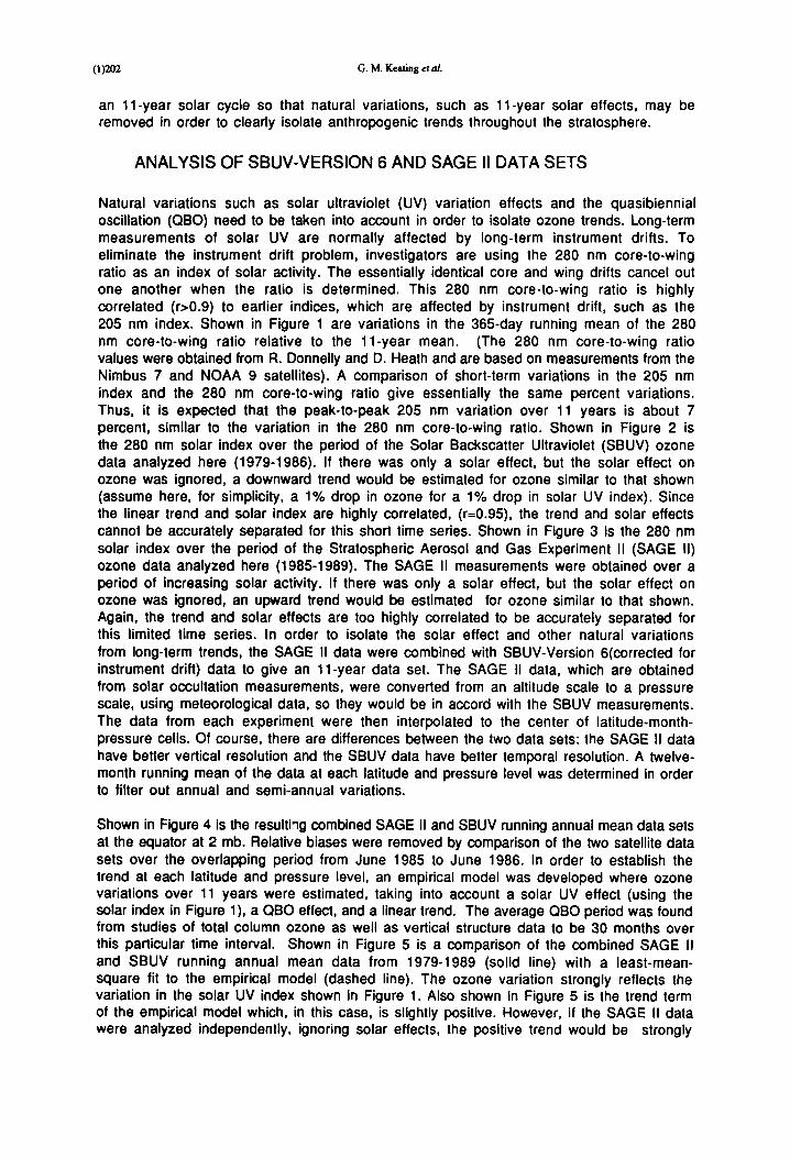
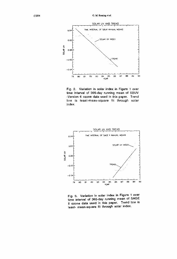
Natural variations such as solar ultraviolet (UV) variation effects and the quasibiennial oscillation (QBO) need to be taken into account in order to isolate ozone trends. Long-term measurements of solar UV are normally affected by long-term instrument drifts. To eliminate the instrument drift problem, investigators are using the 280 nm core-to-wing ratio as an index of solar activity. The essentially identical core and wing drifts cancel out one another when the ratio is determined. This 280 nm core-to-wing ratio is highly correlated (r>0.9) to earlier indices, which are affected by instrument drift, such as the 205 nm index. Shown in Figure 1 are variations in the 365-day running mean of the 280 nm core-to-wing ratio relative to the 11-year mean. (The 280 nm core-to-wing ratio values were obtained from R. Donnelly and D. Heath and are based on measurements from the Nimbus 7 and NOAA 9 satellites). A comparison of short-term variations in the 205 nm index and the 280 nm core-to-wing ratio give essentially the same percent variations. Thus, it is expected that the peak-to-peak 205 nm variation over 11 years is about 7 percent, similar to the variation in the 280 nm core-to-wing ratio. Shown in Figure 2 is the 280 nm solar index over the period of the Solar Backscatter Ultraviolet (SBUV) ozone data analyzed here (1979-1986). If there was only a solar effect, but the solar effect on ozone was ignored, a downward trend would be estimated for ozone similar to that shown (assume here, for simplicity, a 1% drop in ozone for a 1% drop in solar UV index). Since the linear trend and solar index are highly correlated, (r=0.95), the trend and solar effects cannot be accurately separated for this short time series. Shown in Figure 3 is the 280 nm solar index over the period of the Stratospheric Aerosol and Gas Experiment II (SAGE II) ozone data analyzed here (1985-1989). The SAGE II measurements were obtained over a

period of increasing solar activity. If there was only a solar effect, but the solar effect on ozone was ignored, an upward trend would be estimated for ozone similar to that shown. Again, the trend and solar effects are too highly correlated to be accurately separated for this limited time series. In order to isolate the solar effect and other natural variations from long-term trends, the SAGE II data were combined with SBUV-Version 6(corrected for instrument drift) data to give an 11-year data set. The SAGE II data, which are obtained from solar occultation measurements, were converted from an altitude scale to a pressure scale, using meteorological data, so they would be in accord with the SBUV measurements. The data from each experiment were then interpolated to the center of latitude-month- pressure cells. Of course, there are differences between the two data sets: the SAGE II data have better vertical resolution and the SBUV data have better temporal resolution. A twelve- month running mean of the data at each latitude and pressure level was determined in order to filter out annual and semi-annual variations.

Shown in Figure 4 is the resulting combined SAGE II and SBUV running annual mean data sets at the equator at 2 mb. Relative biases were removed by comparison of the two satellite data sets over the overlapping period from June 1985 to June 1986. In order to establish the trend at each latitude and pressure level, an empirical model was developed where ozone variations over 11 years were estimated, taking into account a solar UV effect (using the solar index in Figure 1), a QBO effect, and a linear trend. The average QBO period was found from studies of total column ozone as well as vertical structure data to be 30 months over this particular time interval. Shown in Figure 5 is a comparison of the combined SAGE II and SBUV running annual mean data from 1979-1989 (solid line) with a least-mean- square fit to the empirical model (dashed line). The ozone variation strongly reflects the variation in the solar UV index shown in Figure 1. Also shown in Figure 5 is the trend term of the empirical model which, in this case, is slightly positive. However, if the SAGE II data were analyzed independently, ignoring solar effects, the positive trend would be strongly

Trcmds in Ozom~ Vmical Structure 0)203

0 . 0 7

0.06

0 . 0 5

0 . 0 4

0 . 0 3

0 . 0 2

UV-UV o.o 1 0 . 0 0

- 0 . 0 1

- 0 . 0 2

- 0 . 0 3

- 0 . 0 4 -

- 0 . 0 5 -

- 0 . 0 6 -

- 0 . 0 7

7 6

1 1-YEAR SOLAR UV VARIATION

RESIDUALS IN 3 6 5 - D A Y RUNNING MEAN OF

280 NM CORE-TO-WING RATIO RELATIVE TO

11 -YEAR MEAN I I I I ! I l I l I I l

I I l t i I I I i i i *

79 60 61 62 83 64 65 86 87 86 89 90

YEAR

91

Fig. 1. Variation in 365-day running mean of 280 nm core-to-wing ratio relative to 11- year mean. Data provided by R. Donnelly and D. Heath based on Nimbus 7 and NOAA 9 measurements.

(1)204 G.M. Keating etal.

o.o41

002

~ 000

-O02

SOLAR UV AND TREND

M~ INTEI~VAL OF SBUV ANNUAL MEANS

UV CND£X

- 0 04

79 80 81 • i . l . ] , I , I . . I . l • i . i .

82 83 84 B 5 8 6 87 88 89 90 YEAR

Fig. 2. Variation in solar index in Figure 1 over time interval of 365-day running mean of SBUV -Version 6 ozone data used in this paper. Trend line is least-mean-square fit through solar index.

0.04

0.02

0.00 o

-0.02

-0.04

SOLAR UV AND ]REND

TIME INTE~AL OF ~AGE I I ANNUAL MEANS

, I , i - R . i . i ,

79 80 81

SOLAR UV I N O E X ~

i , i , i , t ,

82 83 84 85 86 87 88 89 90 'fEAR

Fig. 3. Variation in solar index in Figure 1 over time interval of 365-day running mean of SAGE II ozone data used in this paper. Trend line is least- mean-square fit through solar index.

G l o b W T r e n d J i n OzoDe Vertical Structure 0 ) 2 0 5

5.30

5 .20

5.10

v 5.00

o o 4.90

4.80

4.70

78 79 80 81 82 83 84 85 86 87 YEAR

LATITUDE = EQ

T I M E S E R I E S O F S B U V A N D S A G E - I I 2 m b

~ S B U V A N N U A L MEAN /

SAGE II ANNUAL M ~ i k N ~ +

I I OVERLAP • , . i . i . I - | - i . i . l . , . i . i .

68 89 90

Fig. 4. SBUV and SAGE II annual running means in ozone (ppmv) at 2 mb, Equator. The overlap between the two data sets is indicated where relative bias is corrected for.

T I M E S E R I E S O F S B U V A N D S A G E - I t 2 . m b

0 .06 - - " ' " " ' " " - ' " " " ' " ' " "

0 .04 A

"5 0 .02

Eo 0.00

8 • ~ - o . o 2

uJ - 0 . 0 4

- 0 . 0 6

OBSERVATIONS OF ANNUAL MEAN

J - SOLAR UV EFFECT V

- OBO

- 0 . 0 8 . . . , . , , = , , , I , , L , • , - • -

78 80 82 84 86 86 yEAR

LATITUOE - EO

90

Fig. 5. Time series of combined SBUV and SAGE II ozone (fractional variation from overall mean) data at 2 mb, Equator (solid line) compared with an empirical model (dashed line) which includes linear trend, solar UV effect and quasibiennial oscillation (QBO) terms. The trend term, after correction for the solar and QBO effects, is represented by the dotted line.

14:l-H

(I)206 G.M. Ke.ztmg etaL

overestimated. Shown in Figure 6 is the combined SBUV and SAGE II data sets and the empirical model for 2 mb and 10o South. The strong solar effect is obvious again. However, the trend term, represented again as the dotted line, is negative. Similarly, the trends at 20os, 40os, and 50os are found to be negative as represented by Figures 7, 8 and 9 respectively.

GLOBAL TRENDS AND LONG-TERM SOLAR EFFECTS

Shown in Figure 10 is the ozone response to 11-year solar cycle variations (percent ozone change for one percent UV index change) as a function of pressure and latitude based on this study of the combined SBUV and SAGE II data. An unexpectedly strong response is detected near 2 rob. This is a stronger response than the ozone response to 27-day solar UV v3riations (Keating et al., 1987)/1/. A weak response is detected near 8 mb and then another strong response at lower altitudes, which has important effects on total column ozone. This second region of strong response to solar UV variations is located near 30 mb at low latitudes and near 15 mb at mid latitudes.

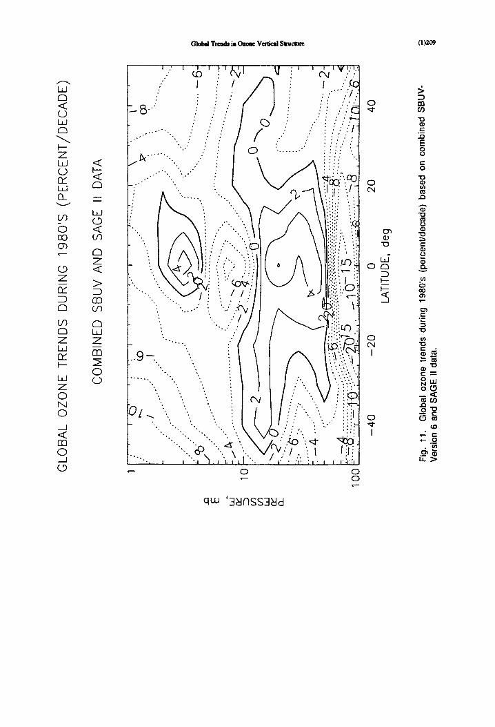
Shown in Figure 11 are the long-term ozone trends (in percent per decade) determined between 1 and 100 mb and between 50os and 50ON after taking into account the solar effects (in Figure 10) and QBO effects. In the upper stratosphere, the depletion rate strongly increases with latitude. This is in general accord with theoretical models which take into account anthropogenic effects. Global trends are seen to be fairly symmetric about the Equator, but are somewhat stronger in the Southern Hemisphere. This may be in part related to the "ozone hole". Near 30 rob, there is evidence of intrusion to mid latitudes of high latitude negative trends. Near 15 mb trends appear to be weak at all latitudes. Near the Equator there appears to be marked stratification of depletion and evidence in some regions of ozone increases. However, uncertainties of the order of 2 percent per decade need to be taken into account.

Near the tropopause there appears to be depletion not just at high latitudes in the Southern Hemisphere but on a global scale. This depletion in ozone in the lower stratosphere may be the result of heterogeneous chemistry somewhat similar to that producing the "ozone hole". On the other hand, considering the altitudinal gradient in ozone near the tropopause, slight increases in tropopause altitude could result in large decreases in ozone mixing ratios. Thus, the depletion near the tropopause may also be related to slight increases with time in tropopause altitude resulting from a cooling ~of the stratosphere. The stratosphere may be cooled by decreases in ozone and increases in carbon dioxide.

It may be concluded that combining the SAGE II and SBUV data sets allows solar effects to be decoupled from trends. This results in detailed information on the stratospheric response to 11-year solar variations and on the nature of ozone depletions as a function of latitude in the upper, middle, and lower stratosphere. With the longer ozone time series which may be available in the future, the decoupling between natural variations and trends may be further improved.

REFERENCES

1. G. M. Keating, M. C. Pitts, G. Brasseur, and A. De Rudder, Response of middle atmosphere to short-term solar ultraviolet variations: 1. Observations, J. Geo~hvs. Res,, 92, 889-902 (1987) .

~"

0.0

4

~E

E

° 0

.02

8 0.

oo

'..T.

~"

--0

.02

-0.0

4

TIM

E

SE

RIE

S

OF

S

BU

V

AN

D

SA

GE

-II

2.

mb

0.0

6

" "

' "

" "

' "

' "

" "

' "

" "

'

OBSE

RVAT

IONS

-0.0

6 -

- •

, .

..

..

..

'

. •

- '

..

..

..

.

78

8

0

82

8

4

B6

8

8

YE

AR

LA

TIT

UO

E

=

I0S

Fig.

6.

Sim

ilar

to F

igur

e 5

but

for

2 m

b an

d 10

os.

O.1

0

A :I

o.o5

E

o

0.0

0

g ~ -0

.05

o

TIM

E

SE

RIE

S

OF

S

BU

V

AN

D

SA

GE

-II

2.

mb

"

" ,

" "

" ,

" -

- |

- •

- l

- -

, -

-

~

OOSE

R'VAT

ION$

..........

..... ~.:

...,.,

......

• .

/s

-0.1

0

. -

- ,

..

..

..

.

, .

. .

, .

. .

, .

. .

78

8

0

82

8

4

86

8

8

go

YE

AR

LA

nT

UO

E

- 4

0S

Fig.

8.

Sim

ilar

to F

igur

e 5

but

for

2 m

b an

d 4

0o

s. g

o

0.0

8

A

0.0

6

"~

0.0

4

E

o '"

0.0

2

8 o 'c

0.~

w

-0.0

2

z o -0

.04

-0.0

6 7

8

TIME SERIES OF SBUV AND SAGE-If

2. mb

:ON

80

8

2

84

8

6

88

9

0

YE

AR

LA

TIT

UD

E

=

2O

S

Fig.

7.

Sim

ilar

to F

igur

e 5

but

for

2 m

b an

d 20

os.

0.151

A

0.10

~E

u2

0.o

5

8 o • c

0.~

-0.0

5

o

TIM

E SE

RIE

S O

F SBUV A

ND S

AG

E-If

2. m

b

~ SE

RVAIIO

NS

-0. I0

- .

- ,

• •

. ,

. •

. I

, .

, 'I

-

- -

= -

- ,

78

80

6

2

84

8

6

00

YE

AR

LA

TIT

UD

E

=

50

S

Fig.

9.

Sim

ilar

to F

igur

e 5

but

for

2 m

b an

d 50

os.

go

.< i

Olo

bol

Ozo

ne

Res

pons

e to

1

1-Y

eo

r S

olor

C

ycle

V

orio

tion

s

( P

erc

en

t O

zon

e

Ch

on

ge

fo

r O

ne

P

erc

en

t U

V

Ch

on

ge

)

Co

mb

ine

d

SB

UV

on

d S

AG

E I

I d

oto

.

..

..

..

..

'

..

..

..

..

.

' .

..

..

.

u.8

- '

..

..

. __

LL

" "

'-:':~

-' "'~

'o

o_

o--f_

ogo

J

~ 1

0

"

• 0.

,:30

_ 0

.20

- 5o

- --

--

.n.'~

9

70 ~

U:

Lu

....

....

T-

:--,

....

....

. ,

....

....

. ,

....

.

0 I 0

2

0

30

40

50

LA

TITU

DE

, d

eg

Fig,

10.

G

loba

l oz

one

resp

onse

to

11-y

ear

sola

r cy

cle

vari

atio

n (p

erce

nt o

zone

cha

nge

for

one

perc

ent c

hang

e in

sol

ar U

V i

ndex

) bas

ed o

n co

mbi

ned

SB

UV

-Ver

sion

6 a

nd S

AG

E I

I dat

a.

GLO

BA

L O

ZON

E T

RE

ND

S

DU

RIN

G 1

980'

S

(PE

RC

EN

T/D

EC

AD

E)

CO

MB

INE

D

SB

UV

AN

D

SA

GE

II

DA

TA

..0 E rY

G)

u)

i,i

rY

0_

10

100 1

,.: '

' (b

' 'i

'~::

3'

""

' '

."""

'"

' ~

'"'

' I'

'

,,

...

.....

%".

..-

.....

. ....

. .....

. '

-"...

.. ...

......

......

.. 6:

' /iii

ii • ~i

...:..-

.

..... ...

.-..

..::.~,

.: +..

.__-...

........

.... y

_

, ....

. ~-.-

:::.:~-

~.-..~

:~-~?

~_:--

-~??~

-+-~?

~?~-~

-~-.~?

i..:---

-:-~

:~.; :

.. ::i ii

ii :::

:::: :

:-: :

:..-

.-~8..

--::----

:--~--~

-:.-..-:

--:-:~i

3 (6

:. 75

...:-

:" ...

... :~

-,~

......

.. -L-

-;-~::~

.::~---'

- ..

.. ,

:::r

"":,

l,-,

;'L.

:;~.

. i--

-.,

..."

7. .

... .,

-.-.-.

-.:i.-

..--..

;.'--v

-~.-'

-"-,-

: __

t,.-,.

,

."",

""

,/ll

i ...

.. b"

.'.-

-40

-20

0

20

4

0

LA

TIT

UD

E,

de

g

Fig.

11

. G

loba

l oz

one

tren

ds

duri

ng

1980

's

(per

cenl

/dec

ade)

ba

sed

on c

ombi

ned

SBU

V-

Vers

ion

6 an

d S

AG

E I

I da

ta.