cost functions - economics · cost functions 1. introduction to thecost function ... constructive...
TRANSCRIPT
COST FUNCTIONS
1. INTRODUCTION TO THE COST FUNCTION
1.1. Understanding and representing technology. Economists are interested in the technology used bythe firm. This is usually represented by a set or a function. For example we might describe the technologyin terms of the input correspondence which maps output vectors in Rm
+ into subsets of 2Rn+ . These subsets
are vectors of inputs that will produce the given output vector. This correspondence is given by
V : Rm+ → 2Rn
+ (1)Alternatively we could represent the technology by a function such as the production function y = f(x1,
x2, . . . , xn)We typically postulate or assume certain properties for various representations of technology. For exam-
ple we typically make the following assumptions on the input correspondence.
1.1.1. V.1 No Free Lunch.a: V(0) = Rn
+
b: 0 6∈ V(y), y > 0.
1.1.2. V.2 Weak Input Disposability. ∀ y ε Rm+ , x ε V (y) and λ ≥ 1 ⇒ λx ε V (y)
1.1.3. V.2.S Strong Input Disposability. ∀ y εRm+ x ε V (y) and x′ ≥ x ⇒ x′ ε V (y)
1.1.4. V.3 Weak Output Disposability. ∀ y ε Rm+ V (y) ⊆ V (θy), 0 ≤ θ ≤ 1.
1.1.5. V.3.S Strong Output Disposability. ∀ y, y′ εRm+ , y′ ≥ y ⇒ V (y′) ⊆ V (y)
1.1.6. V.4 Boundedness for vector y. If ‖y`‖ → +∞ as ` → +∞,
∩+∞`=1 V (y`) = ∅
If y is a scalar,⋂
yε(0,+∞)
V (y) = ∅
1.1.7. V.5 T(x) is a closed set. V: Rm+ → 2R
+n is a closed correspondence.
1.1.8. V.6 Attainability. If x ε V(y), y ≥ 0 and x ≥ 0, the ray {λx: λ ≥ 0} intersects all V(θy), θ ≥ 0.
1.1.9. V.7 Quasi-concavity. V is quasi-concave on Rm+ which means ∀ y, y’ ε Rm
+ , 0 ≤ θ ≤ 1, V(y) ∩ V(y’) ⊆V(θy + (1-θ)y’)
1.1.10. V.8 Convexity of V(y). V(y) is a convex set for all y ε Rm+
1.1.11. V.9 Convexity of T(x). V is convex on Rm+ which means ∀ y, y’ ε Rm
+ , 0 ≤ θ ≤ 1, θV(y)+(1-θ)V(y’) ⊆V(θy+ (1-θ)y’)
Date: October 4, 2005.1
2 COST FUNCTIONS
1.2. Understanding and representing behavior. Economists are also very interested in the behavioral re-lationships that arise from firms’ optimizing decisions. These decisions result in reduced form expressionssuch as supply functions y∗ = x(p, w), input demands x∗ = x(p, w), or Hicksian (cost minimizing) demandfunctions x∗ = x(w, y). One of the most basic of these decisions is the cost minimizing decision.
2. THE COST FUNCTION AND ITS PROPERTIES
2.1. Definition of cost function. The cost function is defined for all possible output vectors and all positiveinput price vectors w = (w1, w2, . . . , wn). An output vector, y, is producible if y belongs to the effectivedomain of V(y), i.e,
Dom V = {y ∈ Rm+ : V (y) 6= ∅}
The cost function does not exist it there is no technical way to produce the output in question. The costfunction is defined by
C(y, w) = minx
{wx : xεV (y)}, y ∈ Dom V, w > 0, (2)
or in the case of a single output
C(w, y) = minx
{wx : f(x) ≥ y} (3)
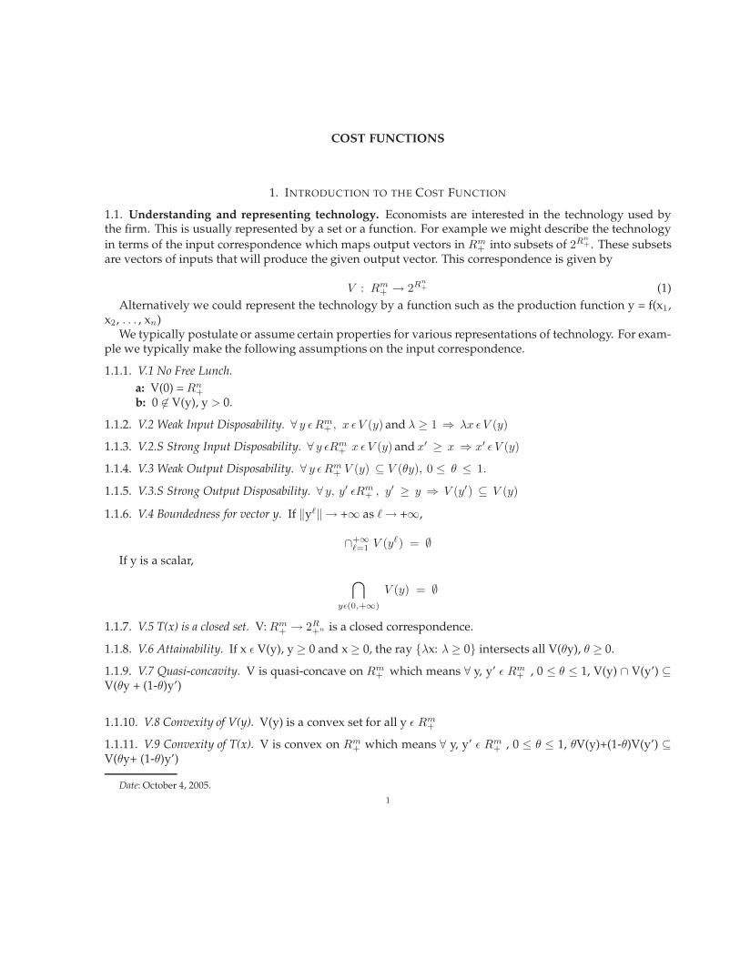
The cost function exists because a continuous function on a nonempty closed bounded set achievesa minimum in the set (Debreu [6, p. 16]). In figure 1,the set V(y) is closed and nonempty for y in theproducible output set. The function wx is continuous. Because V(y) is non-empty if contains at least oneinput bundle x’. We can thus consider cost minimizing points that satisfy wx ≤ wx’ But this set is closedand bounded given that w is strictly positive. Thus the function wx will attain a minimum in the set at x”.
2.2. Solution to the cost minimization problem. The solution to the cost minimization problem 2 is avector x which depends on output vector y and the input vector w. We denote this solution by x(y,w). Thisdemand for inputs at for a fixed level of output and input prices is often called a Hicksian demand curve.
2.3. Properties of the cost function.
2.3.1. C.1.1. Non-negativity: C(y, w) ≥ 0 for w > 0.
2.3.2. C.1.2. Nondecreasing in w: If w ≥ w’ then C(y, w) ≥ C(y, w’)
2.3.3. C.2. Positively linearly homogenous in w
C(y, λw) = λ C(y, w), w > 0.
2.3.4. C.3. C is concave and continuous in w
2.3.5. C.4.1. No fixed costs: C(0, w) = 0, ∀ w > 0. We sometimes assume we have a long run problem.
2.3.6. C.4.2. No free lunch: C(y, w) > 0, w > 0, y > 0.
2.3.7. C.5. Nondecreasing in y (proportional): C(θy, w) ≤ C(y, w), 0 ≤ θ ≤ 1, w > 0.
2.3.8. C.5.S. Nondecreasing in y: C(y’, w) ≤ C(y, w), y’ ≤ y, w > 0.
2.3.9. C.6. For any sequence y` such that || y` || →∞ as ` →∞ and w > 0, C(y`, w) →∞ as ` →∞.
2.3.10. C.7. C(y,w) is lower semi-continuous in y, given w > 0.
COST FUNCTIONS 3
FIGURE 1. Existence of the Cost Function
2.3.11. C.8. If the graph of the technology (GR) or T, is convex, C(y,w) is convex in y, w > 0.
2.4. Discussion of properties of the cost function.
2.4.1. C.1.1. Non-negativity: C(y, w) ≥ 0 for w > 0.
Because it requires inputs to produce an output and w is positive then C(y, w) = wx(y,w) > 0 (y > 0)where x(y,w) is the optimal level of x for a given y.
2.4.2. C.1.2. Nondecreasing in w: If w ≥ w’ then C(y, w) ≥ C(y, w’).
Let w1 ≥ w2. Let x1 be the cost minimizing input bundle with w1 and x2 be the cost minimizing inputbundle with w2. Then w2x2 ≤ w2x1 because x1 is not cost minimizing with prices w2. Now w1x1 ≥ w2x1
because w1 ≥ w2 by assumption so that
C(w1, y) = w1 x1 ≥ w2 x1 ≥ w2 x2 = C(w2, y)
4 COST FUNCTIONS
2.4.3. C.2. Positively linearly homogenous in w
C(y, λw) = λ C(y, w), w > 0.
Let the cost minimization problem with prices w be given by
C(y, w) = minx
{wx : xεV (y)}, y ∈ Dom V, w > 0, (4)
The x vector that solves this problem will be a function of y and w, and is usually denoted x(y,w). Thecost function is then given by
C(y, w) = w x(y, w) (5)
Now consider the problem with prices tw (t >0)
C(y, tw) = minx
{twx : xεV (y)}, y ∈ Dom V, w > 0
= t minx
{wx : xεV (y)}, y ∈ Dom V, w > 0(6)
The x vector that solves this problem will be the same as the vector which solves the problem in equation4, i.e., x(y,w). The cost function for the revised problem is then given by
C(y, tw) = tw x(y, w) = tC(y, w) (7)
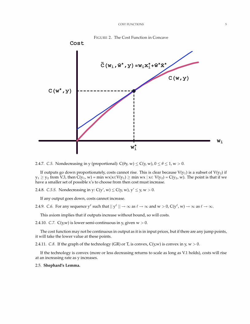
2.4.4. C.3. C is concave and continuous in w
To demonstrate concavity let (w, x) and (w’, x’) be two cost-minimizing price-factor combinations and letw”= tw + (1-t)w’ for any 0 ≤ t ≤ 1. Concavity implies that C(w” y) ≥ tC(w, y) + (1-t) C(w’, y). We can provethis as follows. We have that C(w” y) = w”· x”= tw · x”+ (1-t)w’ · x” where x” is the optimal choice of x atprices w” Because x” is not necessarily the cheapest way to produce y at prices w’ or w,we have w · x”≥C(w, y) and w’· x” ≥ C(w’ y) so that by substitution C(w” y) ≥ tC(w, y) + (1-t) C(w’, y). The point is that if w· x” and w’· x” are each larger than the corresponding term in the linear combination then C(w”,y) is largerthan the linear combination. Because C(y, w)is concave it will be continuous by the property of concavity.Rockafellar [14, p. 82] shows that a concave function defined on an open set (w > 0) is continuous.
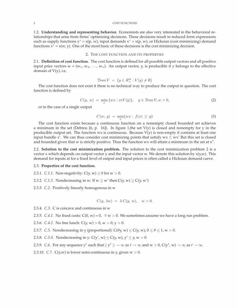
Consider figure 2. Let x∗ be the cost minimizing bundle at prices w∗. Let the price of x∗i change. At input
prices (w∗), costs are at the level C(w∗). If we hold input levels fixed at (x∗) and change wi, we move alongthe tangent line denoted by C(wi, w, y), where w∗ and x∗ represent all the prices and inputs other than theith. Costs are higher along this line than along the cost function because we are not adjusting inputs. Alongthe cost function, as the price of input i increases, we probably use less of input xi and more of other inputs.
2.4.5. C.4.1. No fixed costs: C(0, w) = 0, ∀ w > 0.
We assume this axiom if the problem is long run, in the short run fixed costs may be positive with zerooutput. Specifically V.1a implies that to produce zero output, any input vector in Rn
+ will do, including thezero vector with zero costs.
2.4.6. C.4.2. No free lunch: C(y, w) > 0, w > 0, y > 0.
Because we cannot produce outputs without inputs (V.1b: no free lunch with the technology), costs forany positive output are positive for strictly positive input prices.
COST FUNCTIONS 5
FIGURE 2. The Cost Function in Concave
wi
Cost
CHw,yLC�Hwi,w�*,yL=wixi*+w�*x�*
wi*
CHw*,yL
2.4.7. C.5. Nondecreasing in y (proportional): C(θy, w) ≤ C(y, w), 0 ≤ θ ≤ 1, w > 0.
If outputs go down proportionately, costs cannot rise. This is clear because V(y1) is a subset of V(y2) ify1 ≥ y2 from V.3, then C(y1, w) = min wx|x∈V(y1) ≥ min wx | x∈ V(y2) = C(y2, w). The point is that if wehave a smaller set of possible x’s to choose from then cost must increase.
2.4.8. C.5.S. Nondecreasing in y: C(y’, w) ≤ C(y, w), y’ ≤ y, w > 0.
If any output goes down, costs cannot increase.
2.4.9. C.6. For any sequence y` such that || y` || →∞ as ` →∞ and w > 0, C(y`, w) →∞ as ` →∞.
This axiom implies that if outputs increase without bound, so will costs.
2.4.10. C.7. C(y,w) is lower semi-continuous in y, given w > 0.
The cost function may not be continuous in output as it is in input prices, but if there are any jump points,it will take the lower value at these points.
2.4.11. C.8. If the graph of the technology (GR) or T, is convex, C(y,w) is convex in y, w > 0.
If the technology is convex (more or less decreasing returns to scale as long as V.1 holds), costs will riseat an increasing rate as y increases.
2.5. Shephard’s Lemma.
6 COST FUNCTIONS
2.5.1. Definition of Shephard’s lemma. In the case where V is strictly quasi-concave and V(y) is strictly convexthe cost minimizing point is unique. Rockafellar [14, p. 242] shows that the cost function is differentiablein w, w > 0 at (y,w) if and only if the cost minimizing set of inputs at (y,w) is a singleton, i.e., the costminimizing point is unique. In such cases.
∂C(y, w)∂wi
= xi(y, w) (8)
which is the Hicksian Demand Curve. As with Hotelling’s lemma in the case of the profit function, thislemma allows us to obtain the input demand functions as derivatives of the cost function.
2.5.2. Constructive proof of Shephard’s lemma in the case of a single output. For a single output, the cost mini-mization problem is given by
C(y, w) = minx
wx : f(x) − y = 0 (9)
The associated Lagrangian is given by
L = wx − λ(f(x) − y) (10)The first order conditions are as follows
∂L
∂xi= wi − λ
∂f
∂xi= 0, i = 1, . . . , n (11a)
∂L
∂λ= − (f(x) − y) = 0 (11b)
Solving for the optimal x’s yields
xi(y, w) (12)with C(y,w) given by
C(w, y) = wx(y, w) (13)If we now differentiate 13 with respect to w we obtain
∂C
∂wi= Σn
j=1 wj∂xj(y, w)
∂wi+ xi (y, w) (14)
From the first order conditions in equation 11a (assuming that the constraint is satisfied as an equality)we have
wj = λ∂f
∂xj(15)
Substitute the expression for wj from equation 15 into equation 14 to obtain
∂C
∂wi= Σn
j=1 λ∂f(x)∂xj
∂xj (y, w)∂wi
+ xi (y, w) (16)
If λ > 0 then equation 11b implies(f(x)-y) = 0. Now differentiate equation 11b with respect to wi to obtain
Σnj=1
∂f(x(y, w))∂xj
∂xj (y, w)∂wi
= 0 (17)
which implies that the first term in equation 16 is equal to zero and that
COST FUNCTIONS 7
∂C(y, w)∂wi
= xi (y, w) (18)
2.5.3. A Silberberg [17] type proof of Shephard’s lemma. Set up a function L as follows
L(y, w, x) = w x − C(w, y) (19)
where x is the cost minimizing choice of inputs for prices w. Because C(w, y) is the cheapest way toproduce y at prices w, L ≥ 0. If w = w, then L will be equal to zero. Because this is the minimum value of L,the derivative of L at this point is zero so
∂L(y, w, x)∂wi
= xi − ∂C(w, y)∂wi
= 0
⇒ xi =∂C(w, y)
∂wi
(20)
The second order necessary conditions for minimizing L imply that[
−∂2C
∂wi∂wj
](21)
is positive semi-definite so that
∂2 C
∂wi ∂wj(22)
is negative semi-definite which implies that C is concave.
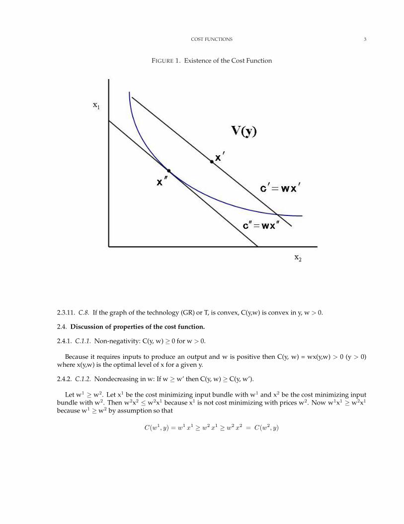
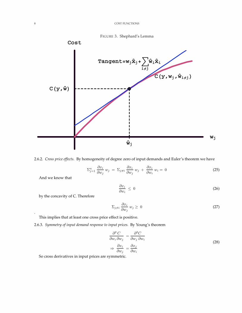
2.5.4. Graphical representation of Shephard’s lemma. In figure 3 we hold all input prices except the jth fixed atw. We assume that when the jth price is wj, the optimal input vector is (x1, x2, . . . , xj, . . . ,xn). The costfunction lies below the tangent line in figure 3 but conincides with the tangent line at wj By differentiabilitythe slope of the cost function at this point is the slope of its tangent i.e.,
∂C
∂wj=
∂(tangent)∂wj
= xj (23)
2.6. Sensitivity analysis.
2.6.1. Demand slopes. If the Hessian of the cost function is negative semi-definite, the diagonal elements allmust be non-positive(Hadley [11, p. 260-262]) so we have
∂2 C(y, w)∂w2
i
=∂xi (y, w)
∂wi≤ 0 ∀i (24)
This implies then that Hicksian demand curves slope down because the diagonal elements of the Hessianof the cost function are just the derivatives of input demands with respect to their own prices.
8 COST FUNCTIONS
FIGURE 3. Shephard’s Lemma
wj
Cost
CHy,wj,wi¹jLTangent=wjxj+â
i¹j
wixi
wj
CHy,wL
2.6.2. Cross price effects. By homogeneity of degree zero of input demands and Euler’s theorem we have
Σnj=1
∂xi
∂wjwj = Σj 6=i
∂xi
∂wjwj +
∂xi
∂wiwi = 0 (25)
And we know that
∂xi
∂wi≤ 0 (26)
by the concavity of C. Therefore
Σj 6=i∂xi
∂wjwj ≥ 0 (27)
.This implies that at least one cross price effect is positive.
2.6.3. Symmetry of input demand response to input prices. By Young’s theorem
∂2 C
∂wi ∂wj=
∂2C
∂wj ∂wi
⇒ ∂xi
∂wj=
∂xj
∂wi
(28)
So cross derivatives in input prices are symmetric.
COST FUNCTIONS 9
2.6.4. Marginal cost. Consider the first order conditions for cost minimization. If we differentiate 13 withrespect to y we obtain
∂C
∂y= Σn
j=1 wj∂xj(y, w)
∂y(29)
From the first order conditions in equation 11a (assuming that the constraint is satisfied as an equality)we have
wj = λ∂f
∂xj(30)
Substitute the expression for wj from equation 30 into equation 29 to obtain
∂C
∂y= Σn
j=1 λ∂f(x)∂xj
∂xj (y, w)∂y
= λ Σnj=1
∂f(x)∂xj
∂xj (y, w)∂y
(31)
If λ > 0 then equation 11b implies(f(x)-y) = 0. Now differentiate equation 11b (ignoring λ) with respectto y to obtain
Σnj=1
∂f(x(y, w))∂xj
∂xj (y, w)∂y
− 1 = 0
⇒ Σnj=1
∂f(x(y, w))∂xj
∂xj (y, w)∂y
= 1
(32)
This then implies that the first term in equation 16 that
∂C(y, w)∂y
= λ (y, w) (33)
The Lagrangian multiplier from the cost minimization problem is equal to marginal cost or the increasein cost from increasing the targeted level of y in the constraint.
2.6.5. Symmetry of input demand response to changes in output and changes in marginal cost with respect to inputprices. Remember that
∂2 C
∂y ∂wi=
∂2C
∂wi ∂y(34)
This then implies that
∂xi
∂y=
∂λ
∂wi(35)
The change in xi(y, w) from an increase in y equals the change in marginal cost due to an increase in wi.
2.6.6. Marginal cost is homogeneous of degree one in input prices. Marginal cost is homogeneous of degree onein input prices.
∂C (ty, w)∂y
= t∂C(y, w)
∂y, t > 0. (36)
We can show using the Euler equation. If a function is homogeneous of degree one, then
10 COST FUNCTIONS
Σni=1
∂f
∂xixi = f(x) (37)
Applying this to marginal cost we obtain
∂MC(y, w)∂wi
=∂λ(y, w)
∂wi=
∂2 C(y, w)∂wi ∂y
=∂2 C(y, w)
∂y ∂wi=
∂ xi(y, w)∂y
⇒ Σi∂λ(y, w)
∂wiwi = Σi
∂2 C(y, w)∂wi ∂y
wi = Σi∂2 C(y, w)
∂y ∂wiwi
=∂
∂y
(Σi
∂ C(y, w)∂wi
wi
)
=∂
∂yC(y, w ), by homogeneity of C(y,w) in w
= MC(y, w) = λ(y, w)
(38)
COST FUNCTIONS 11
3. TRADITIONAL APPROACH TO THE COST FUNCTION
3.1. First order conditions for cost minimization. In the case of a single output, the cost function can beobtained by carrying out the maximization problem
C(y, w) = minx
wx : f(x) − y = 0 (39)
with associated Lagrangian function
L = wx − λ(f(x) − y) (40)The first order conditions are as follows
∂L
∂x1= w1 − λ
∂f
∂x1= 0
∂L
∂x2= w2 − λ
∂f
∂x2= 0
......
∂L
∂xn= wn − λ
∂f
∂xn= 0
(41a)
∂λ
∂λ= − (f(x) − y) = 0 (41b)
If we take the ratio of any of the first order conditions we obtain
∂f∂xj
∂f∂xi
=wj
wi(42)
This implies that the RTS between inputs i and j is equal to the negative inverse factor price ratio because
RTS =∂xi
∂xj=
− ∂f∂xj
∂f∂xi
(43)
Substituting we obtain
RTS =∂xi
∂xj= −wj
wi(44)
Graphically this implies that the slope of an isocost line is equal to the slope of the lower boundary ofV(y). Note that an isocost line is given by
cost = w1 x1 + w2 x2 + . . . + wn xn
⇒ wi xi = cost − w1 x1 − w2 x2 − . . . − wi−1 xi−1 − wi+1 xi+1 − . . . − wj xj − . . . − wn xn
⇒ xj =cost
wi− w1
wix1 − w2
wix2 − . . . − wi−1
wixi−1 − wi+1
wixi+1 − . . . − wj
wixj − . . . − wn
wixn
⇒ Slope of isocost = − wj
wi(45)
12 COST FUNCTIONS
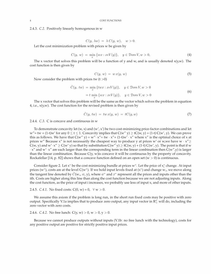
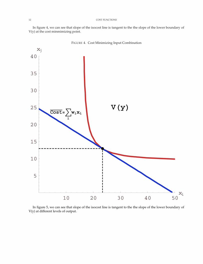
In figure 4, we can see that slope of the isocost line is tangent to the the slope of the lower boundary ofV(y) at the cost minmimizing point.
FIGURE 4. Cost Minimizing Input Combination
10 20 30 40 50xi
5
10
15
20
25
30
35
40xj
VHyLCost���������
=âi
wixi
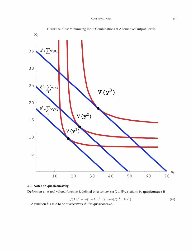
In figure 5, we can see that slope of the isocost line is tangent to the the slope of the lower boundary ofV(y) at different levels of output.
COST FUNCTIONS 13
FIGURE 5. Cost Minimizing Input Combinations at Alternative Output Levels
10 20 30 40 50 60 70xi
5
10
15
20
25
30
35
xj
VHy3LVHy2L
VHy1L
C�2=â
i
wixi
C�1=â
i
wixi
C�3=â
i
wixi
3.2. Notes on quasiconcavity.
Definition 1. A real valued function f, defined on a convex set X ⊂ <n, a said to be quasiconcave if
f( λ x1 + +(1 − λ) x2) ≥ min[f(x1), f(x2) ] (46)A function f is said to be quasiconvex if - f is quasiconcave.
14 COST FUNCTIONS
Theorem 1. Let f be a real valued function defined on a convex set X ⊂ Rn. The upper contour sets {(x, y): x ∈ S, α≤ f(x)} of f are convex for every α ∈ R if and only if f is a quasiconcave function.
Proof. Suppose that S(f,α) is a convex set for every α ∈ R and let x1 ∈ X, x2 ∈ X, α = min[f(x1), f(x2)]. Thenx1 ∈ S(f,α) and x2 ∈ S(f,α), and because S(f,α) is convex, (λx1 + (1-λ)x2) ∈ S(f,α) for arbitrary λ. Hence
f(λ x1 + (1 − λ) x2) ≥ α = min[f(x1), f(x2) ] (47)Conversely, let S(f,α) be any level set of f. Let x1 ∈ S(f,α) and x2 ∈ S(f,α). Then
f(x1) ≥ α, f(x2) ≥ α (48)and because f is quasiconcave, we have
f(λ x1 + (1 − λ) x2) ≥ α (49)and (λx1 + (1-λ) x2) ∈ S(f,α).
�
Theorem 2. Let f be differentiable on an open convex set X ⊂ Rn. Then f is quasiconcave if and only if for any x1 ∈X, x2 ∈ X such that
f(x1) ≥ f(x2) (50)we have
(x1 − x2)′ ∇f(x2) ≥ 0 (51)
Definition 2. The kth-ordered bordered determinant Dk(f,x) of a twice differentiable function f at at pointx ∈ Rn is defined as
Dk(f, x) = det
∂2f∂x2
1
∂2f∂x1∂x2
· · · ∂2f∂x1∂xk
∂f∂x1
∂2f∂x2∂x1
∂2f∂x2
2· · · ∂2f
∂x2∂xk
∂f∂x2
......
......
∂2f∂xk∂x1
∂2f∂xk∂x2
· · · ∂2f∂x2
k
∂f∂xk
∂f∂x1
∂f∂x2
· · · ∂f∂xk
0
k = 1, 2, . . . , n (52)
Definition 3. Some authors define the kth-ordered bordered determinant Dk(f,x) of a twice differentiablefunction f at at point x ∈ Rn in a different fashion where the first derivatives of the function f border theHessian of the function on the top and left as compared to in the bottom and right as in equation 52.
Dk(f, x) = det
0 ∂f∂x1
∂f∂x2
· · · ∂f∂xk
∂f∂x1
∂2f∂x2
1
∂2f∂x1∂x2
· · · ∂2f∂x1∂xk
∂f∂x2
∂2f∂x2∂x1
∂2f∂x2
2· · · ∂2f
∂x2∂xk
......
......
∂f∂xk
∂2f∂xk∂x1
∂2f∂xk∂x2
· · · ∂2f∂x2
k
k = 1, 2, . . . , n (53)
The determinant in equation 52 and the determinant in equation 53 will be the same. If we interchangeany two rows or any two columns of a determinant, the determinant will change sign but keep its absolute
COST FUNCTIONS 15
value. A certain number of row exchanges will be necessary to move the bottom row to the top. A likenumber of column exchanges will be necessary to move the rightmost column to the left. Given that equa-tions 52 and 53 are the same except for this even number of row and column exchanges, the determinantswill be the same. You can illustrate this to yourself using the following three variable example.
HB =
∂2f∂x2
1
∂2f∂x1∂x2
∂2f∂x1∂x3
∂f∂x1
∂2f∂x2∂x1
∂2f∂x2
2
∂2f∂x2∂x3
∂f∂x2
∂2f∂x3∂x1
∂2f∂x3∂x2
∂2f∂x2
3
∂f∂x3
∂f∂x1
∂f∂x2
∂f∂x3
0
HB =
0 ∂f∂x1
∂f∂x2
∂f∂x3
∂f∂x1
∂2f∂x2
1
∂2f∂x1∂x2
∂2f∂x1∂x3
∂f∂x2
∂2f∂x2∂x1
∂2f∂x2
2
∂2f∂x2∂x3
∂f∂x3
∂2f∂x3∂x1
∂2f∂x3∂x2
∂2f∂x2
3
3.2.1. Quasi-concavity and bordered hessians.a.: If f(x) is quasi-concave on a solid (non-empty interior) convex set X ⊂ Rn, then
(−1)k Dk(f, x) ≥ 0, k = 1, 2, . . . , n (54)for every x ∈ X.
b.: If
(−1)k Dk(f, x) > 0, k = 1, 2, . . . , n (55)for every x ∈ X,then f(x) is quasi-concave on X (Avriel [3, p.149], Arrow and Enthoven [2, p.
781-782]If f is quasiconcave, then when k is odd, Dk(f,x) will be negative and when k is even, Dk(f,x) will be
positive. Thus Dk(f,x)will alternate in sign beginning with positive in the case of two variables.
3.2.2. Relationship of quasi-concavity to signs of minors (cofactors) of a matrix. Let
F =
∣∣∣∣∣∣∣∣∣∣∣∣∣∣∣
0 ∂f∂x1
∂f∂x2
· · · ∂f∂xn
∂f∂x1
∂2f∂x2
1
∂2f∂x1∂x2
· · · ∂2f∂x1∂xn
∂f∂x2
∂2f∂x2∂x1
∂2f∂x2
2· · · ∂2f
∂x2∂xn
......
......
∂f∂xn
∂2f∂xn∂x1
∂2f∂xn∂x2
· · · ∂2f∂x2
n
∣∣∣∣∣∣∣∣∣∣∣∣∣∣∣
= det HB (56)
where det HB is the determinant of the bordered Hessian of the function f. Now let Fij be the cofactor of∂2f
∂xi∂xjin the matrix HB . It is clear that Fnn and F have opposite signs because F includes the last row and
column of HB and Fnn does not. If the (-1)n in front of the cofactors is positive then Fnn must be positivewith F negative and vice versa. Since the ordering of rows since is arbitrary it is also clear that Fii and Fhave opposite signs. Thus when a function is quasi-concave Fii
F will have a negative sign.
3.3. Second order conditions for cost minimization.
3.3.1. Note on requirements for a minimum of a constrained problem. Consider a general constrained optimiza-tion problem with one constraint.
maximizex
f(x)
subject to g(x) = 0
16 COST FUNCTIONS
where g(x) = 0 denotes a constraint, We can also write this as
maxx1, x2,...xn
f(x1, x2, . . . , xn)
subject tog (x1, x2, . . . , xn) = 0 (57)
The solution can be obtained using the Lagrangian function
L(x; λ) = f(x1, x2, . . .) − λ g(x) (58)
Notice that the gradient of L will involve a set of derivatives, i.e.
∇x L = ∇xf(x) − λ∇xg(x)
There will be one equation for each x. There will also an equation involving the derivative of L withrespect to λ. The necessary conditions for an extremum of f with the equality constraints g(x) = 0 are that
∇L(x∗, λ∗) = 0 (59)
where it is implicit that the gradient in (59) is with respect to both x and λ. The typical sufficient con-ditions for a maximum or minimum of f(x1, x2, . . . , xn) subject to g(x1, x2,. . . , xn) = 0 require that f and gbe twice continuously differentiable real-valued functions on Rn. Then if there exist vectors x∗ ∈ Rn, andλ∗ ∈ R1 such that
∇L(x∗, λ∗) = 0 (60)
and for every non-zero vector z ∈ Rn satisfying
z′∇g(x∗) = 0 (61)
it follows that
z′∇2x L(x∗, λ∗)z > 0 (62)
then f has a strict local minimum at x∗, subject to g(x) = 0. If the inequality in (62) is reversed, then fhas strict local maximum at x∗.
For the cost minimization problem the Lagrangian is given by
L = wx − λ(f(x) − y) (63)
where the objective function is wx and the constraint is f(x) - y = 0. Differentiating equation 63 twicewith respect to x we obtain
∇2x L(x∗, λ∗) =
[−λ
∂2f(x)∂xi ∂xj
]
= − λ
[∂2f(x)∂xi ∂xj
] (64)
And so the condition in equation 62 will imply that
COST FUNCTIONS 17
−λ z′[
∂2f(x)∂xi∂xj
]z > 0
⇒ z′[
∂2f(x)∂xi∂xj
]z < 0
(65)
for all z satisfying z’∇f(x) = 0. This is also the condition for f to be a quasi-concave function. (Avriel [3,p.149]. Thus these sufficient conditions imply that f must be quasi-concave.
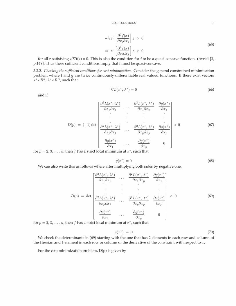
3.3.2. Checking the sufficient conditions for cost minimization. Consider the general constrained minimizationproblem where f and g are twice continuously differentiable real valued functions. If there exist vectorsx∗ ε Rn, λ∗ ε Rm, such that
∇L(x∗, λ∗) = 0 (66)and if
D(p) = (−1) det
∂2L(x∗, λ∗)∂x1∂x1
. . .∂2L(x∗, λ∗)
∂x1∂xp
∂g(x∗)∂x1
· · · ·· · · ·· · · ·
∂2L(x∗, λ∗)∂xp∂x1
. . .∂2L(x∗, λ∗)
∂xp∂xp
∂g(x∗)∂xp
∂g(x∗)∂x1
. . .∂g(x∗)∂xp
0
> 0 (67)
for p = 2, 3, . . . , n, then f has a strict local minimum at x∗, such that
g(x∗) = 0 (68)We can also write this as follows where after multiplying both sides by negative one.
D(p) = det
∂2L(x∗, λ∗)∂x1∂x1
. . .∂2L(x∗, λ∗)
∂x1∂xp
∂g(x∗)∂x1
· · · ·· · · ·· · · ·
∂2L(x∗, λ∗)∂xp∂x1
. . .∂2L(x∗, λ∗)
∂xp∂xp
∂g(x∗)∂xp
∂g(x∗)∂x1
. . .∂g(x∗)∂xp
0
< 0 (69)
for p = 2, 3, . . . , n, then f has a strict local minimum at x∗, such that
g(x∗) = 0 (70)We check the determinants in (69) starting with the one that has 2 elements in each row and column of
the Hessian and 1 element in each row or column of the derivative of the constraint with respect to x.
For the cost minimization problem, D(p) is given by
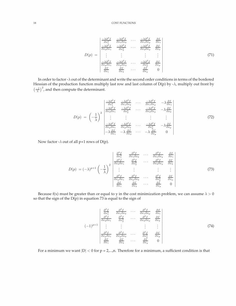
18 COST FUNCTIONS
D(p) =
∣∣∣∣∣∣∣∣∣∣∣∣∣∣∣
−λ∂2f∂x2
1
−λ∂2f∂x1∂x2
· · · −λ∂2f∂x1∂xp
∂f∂x1
−λ∂2f∂x2∂x1
−λ∂2f∂x2
2· · · −λ∂2f
∂x2∂xp
∂f∂x2
......
......
−λ∂2f∂xp∂x1
−λ∂2f∂xp∂x2
· · · −λ∂2f∂x2
p
∂f∂xp
∂f∂x1
∂f∂x2
· · · ∂f∂xp
0
∣∣∣∣∣∣∣∣∣∣∣∣∣∣∣
(71)
In order to factor -λ out of the determinant and write the second order conditions in terms of the borderedHessian of the production function multiply last row and last column of D(p) by -λ, multiply out front by(−1
λ
)2, and then compute the determinant.
D(p) =(− 1
λ
)2
∣∣∣∣∣∣∣∣∣∣∣∣∣∣∣
−λ∂2f∂x2
1
−λ∂2f∂x1∂x2
· · · −λ∂2f∂x1∂xp
−λ ∂f∂x1
−λ∂2f∂x2∂x1
−λ∂2f∂x2
2· · · −λ∂2f
∂x2∂xp−λ ∂f
∂x2
......
......
−λ∂2f∂xp∂x1
−λ∂2f∂xp∂x2
· · · −λ∂2f∂x2
p−λ ∂f
∂xp
−λ ∂f∂x1
−λ ∂f∂x2
· · · −λ ∂f∂xp
0
∣∣∣∣∣∣∣∣∣∣∣∣∣∣∣
(72)
Now factor -λ out of all p+1 rows of D(p).
D(p) = (−λ)p+1
(− 1
λ
)2
∣∣∣∣∣∣∣∣∣∣∣∣∣∣∣
∂2f∂x2
1
∂2f∂x1∂x2
· · · ∂2f∂x1∂xp
∂f∂x1
∂2f∂x2∂x1
∂2f∂x2
2· · · ∂2f
∂x2∂xp
∂f∂x2
......
......
∂2f∂xp∂x1
∂2f∂xp∂x2
· · · ∂2f∂x2
p
∂f∂xp
∂f∂x1
∂f∂x2
· · · ∂f∂xp
0
∣∣∣∣∣∣∣∣∣∣∣∣∣∣∣
(73)
Because f(x) must be greater than or equal to y in the cost minimization problem, we can assume λ > 0so that the sign of the D(p) in equation 73 is equal to the sign of
(−1)p+1
∣∣∣∣∣∣∣∣∣∣∣∣∣∣∣
∂2f∂x2
1
∂2f∂x1∂x2
· · · ∂2f∂x1∂xp
∂f∂x1
∂2f∂x2∂x1
∂2f∂x2
2· · · ∂2f
∂x2∂xp
∂f∂x2
......
......
∂2f∂xp∂x1
∂2f∂xp∂x2
· · · ∂2f∂x2
p
∂f∂xp
∂f∂x1
∂f∂x2
· · · ∂f∂xp
0
∣∣∣∣∣∣∣∣∣∣∣∣∣∣∣
(74)
For a minimum we want |D| < 0 for p = 2,...,n. Therefore for a minimum, a sufficient condition is that
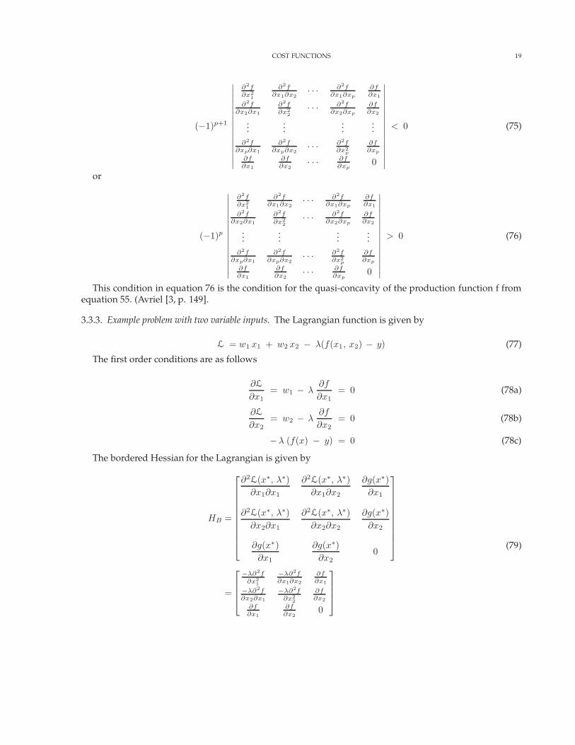
COST FUNCTIONS 19
(−1)p+1
∣∣∣∣∣∣∣∣∣∣∣∣∣∣∣
∂2f∂x2
1
∂2f∂x1∂x2
· · · ∂2f∂x1∂xp
∂f∂x1
∂2f∂x2∂x1
∂2f∂x2
2· · · ∂2f
∂x2∂xp
∂f∂x2
......
......
∂2f∂xp∂x1
∂2f∂xp∂x2
· · · ∂2f∂x2
p
∂f∂xp
∂f∂x1
∂f∂x2
· · · ∂f∂xp
0
∣∣∣∣∣∣∣∣∣∣∣∣∣∣∣
< 0 (75)
or
(−1)p
∣∣∣∣∣∣∣∣∣∣∣∣∣∣∣
∂2f∂x2
1
∂2f∂x1∂x2
· · · ∂2f∂x1∂xp
∂f∂x1
∂2f∂x2∂x1
∂2f∂x2
2· · · ∂2f
∂x2∂xp
∂f∂x2
......
......
∂2f∂xp∂x1
∂2f∂xp∂x2
· · · ∂2f∂x2
p
∂f∂xp
∂f∂x1
∂f∂x2
· · · ∂f∂xp
0
∣∣∣∣∣∣∣∣∣∣∣∣∣∣∣
> 0 (76)
This condition in equation 76 is the condition for the quasi-concavity of the production function f fromequation 55. (Avriel [3, p. 149].
3.3.3. Example problem with two variable inputs. The Lagrangian function is given by
L = w1 x1 + w2 x2 − λ(f(x1, x2) − y) (77)
The first order conditions are as follows
∂L
∂x1= w1 − λ
∂f
∂x1= 0 (78a)
∂L
∂x2= w2 − λ
∂f
∂x2= 0 (78b)
−λ (f(x) − y) = 0 (78c)
The bordered Hessian for the Lagrangian is given by
HB =
∂2L(x∗, λ∗)∂x1∂x1
∂2L(x∗, λ∗)∂x1∂x2
∂g(x∗)∂x1
∂2L(x∗, λ∗)∂x2∂x1
∂2L(x∗, λ∗)∂x2∂x2
∂g(x∗)∂x2
∂g(x∗)∂x1
∂g(x∗)∂x2
0
=
−λ∂2f∂x2
1
−λ∂2f∂x1∂x2
∂f∂x1
−λ∂2f∂x2∂x1
−λ∂2f∂x2
2
∂f∂x2
∂f∂x1
∂f∂x2
0
(79)
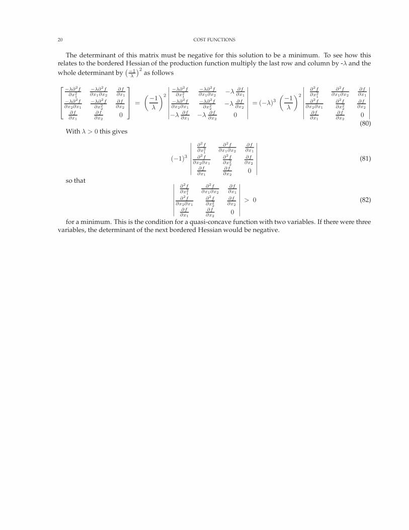
20 COST FUNCTIONS
The determinant of this matrix must be negative for this solution to be a minimum. To see how thisrelates to the bordered Hessian of the production function multiply the last row and column by -λ and thewhole determinant by
(−1λ
)2 as follows
−λ∂2f∂x2
1
−λ∂2f∂x1∂x2
∂f∂x1
−λ∂2f∂x2∂x1
−λ∂2f∂x2
2
∂f∂x2
∂f∂x1
∂f∂x2
0
=
(−1λ
)2
∣∣∣∣∣∣∣∣
−λ∂2f∂x2
1
−λ∂2f∂x1∂x2
−λ ∂f∂x1
−λ∂2f∂x2∂x1
−λ∂2f∂x2
2−λ ∂f
∂x2
−λ ∂f∂x1
−λ ∂f∂x2
0
∣∣∣∣∣∣∣∣= (−λ)3
(−1λ
)2
∣∣∣∣∣∣∣∣
∂2f∂x2
1
∂2f∂x1∂x2
∂f∂x1
∂2f∂x2∂x1
∂2f∂x2
2
∂f∂x2
∂f∂x1
∂f∂x2
0
∣∣∣∣∣∣∣∣(80)
With λ > 0 this gives
(−1)3
∣∣∣∣∣∣∣∣
∂2f∂x2
1
∂2f∂x1∂x2
∂f∂x1
∂2f∂x2∂x1
∂2f∂x2
2
∂f∂x2
∂f∂x1
∂f∂x2
0
∣∣∣∣∣∣∣∣(81)
so that ∣∣∣∣∣∣∣∣
∂2f∂x2
1
∂2f∂x1∂x2
∂f∂x1
∂2f∂x2∂x1
∂2f∂x2
2
∂f∂x2
∂f∂x1
∂f∂x2
0
∣∣∣∣∣∣∣∣> 0 (82)
for a minimum. This is the condition for a quasi-concave function with two variables. If there were threevariables, the determinant of the next bordered Hessian would be negative.
COST FUNCTIONS 21
3.4. Input demands. If we solve the equations in 41 for xj , j = 1, 2, . . ., n, and λ, we obtain the optimalvalues of x for a given y and w. As a function of w for a fixed y, this gives the vector of factor demands forx and the optimal Lagrangian multiplier λ(y,w).
x = x(y, w) = (x1(y, w), x2(y, w), . . . , xn(y, w))
λ = λ(y, w)(83)
3.5. Sensitivity analysis. We can investigate the properties of x(y,w) by substituting x(y,w) for x in equa-tion 41 and then treating it as an identity.
∂L
∂x1= w1 − λ
∂f(x1(y, w), x2(y, w), . . . , xn(y, w))∂x1
= 0
∂L
∂x2= w2 − λ
∂f(x1(y, w), x2(y, w), . . . , xn(y, w))∂x2
= 0
......
∂L
∂xn= wn − λ
∂f(x1(y, w), x2(y, w), . . . , xn(y, w))∂xn
= 0
(84a)
−λ (f((x1(y, w), x2(y, w), . . . , xn(y, w)) − y) = 0 (84b)
Where it is obvious we write x(y,w) for x(y,w) and xj(y,w) for xj(y,w). If we differentiate the first equationin 84a with respect to wj we obtain
0 − λ
(∂2f(x(y, w))
∂x21
∂x1(y, w)
∂wj+
∂2f(x(y,w))
∂x2 ∂x1
∂x2(y, w)
∂wj+
∂2f(x(y,w))
∂x3∂x1
∂ x3(y,w)
∂wj+ · · ·
)− ∂f(x(y, w))
∂x1
∂λ(y, w)
∂wj≡ 0
⇒ λ(
∂2f(x(y, w))
∂x21
∂2f(x(y,w))∂x2 ∂x1
∂2f(x(y,w))∂x3∂x1
· · · ∂2f(x(y,w))∂xn∂x1
∂f(x(y, w))∂x1
)
∂x1(y, w)∂wj
∂x2(y, w)∂wj
∂x3(y, w)∂wj
...∂xn(y, w)
∂wj
1λ
∂λ(y, w)∂wj
≡ 0
(85)If we differentiate the second equation in 84a with respect to wj we obtain
22 COST FUNCTIONS
0 − λ
(∂2f(x(y, w))
∂x1∂x2
∂x1(p, w)
∂wj+
∂2f(x(y,w))
∂x22
∂x2(y,w)
∂wj+
∂2f(x(y,w))
∂x3∂x2
∂ x3(y, w)
∂wj+ · · ·
)− ∂f(x(y, w))
∂x2
∂λ(y, w)
∂wj≡ 0
⇒ λ(
∂2f(x(y, w))∂x1 ∂x2
∂2f(x(y,w))
∂x22
∂2f(x(y,w))∂x3∂x2
· · · ∂2f(x(y,w))∂xn∂x2
∂f(x(y, w))∂x2
)
∂x1(y, w)∂wj
∂x2(y, w)∂wj
∂x3(y, w)∂wj
...∂xn(y, w)
∂wj
1λ
∂λ(y, w)∂wj
≡ 0
(86)If we differentiate the jth equation in 84a with respect to wj we obtain
1 − λ
∂2f(x(y, w))
∂x1∂xj
∂x1(y, w)
∂wj
+∂2f(x(y, w))
∂x2 ∂xj
∂x2(y, w)
∂wj
+ · · · +∂2f(x(y, w))
∂x2j
∂ xj (y, w)
∂wj
+ · · ·
−
∂f(x(y, w))
∂xj
∂λ(y, w)
∂wj
≡ 0
⇒ λ
(∂2f(x(y, w))
∂x1 ∂xj
∂2f(x(y,w))∂x2 ∂xj
· · · ∂2f(x(y,w))∂x2
j
· · · ∂2f(x(y,w)∂xn∂xj
∂f(x(y, w))∂xj
)
∂x1(y, w)∂wj
∂x2(y, w)∂wj
∂x3(y, w)∂wj
.
.
.∂xn(y, w)
∂wj1λ
∂λ(y, w)∂wj
≡ 1
(87)
Continuing in the same fashion we obtain
λ
∂2f(x(y, w))∂x2
1
∂2f(x(y,w)∂x2 ∂x1
· · · ∂2f(x(y,w)∂xj∂x1
· · · ∂2f(x(y,w)∂xn∂x1
∂f(x(y,w)∂x1
∂2f(x(y, w))∂x1∂x2
∂2f(x(y,w)∂x2
2· · · ∂2f(x(y,w)
∂xj∂x2· · · ∂2f(x(y,w)
∂xn∂x2
∂f(x(y,w)∂x2
......
......
......
∂2f(x(y, w))∂x1∂xj
∂2f(x(y,w)∂x2∂xj
· · · ∂2f(x(y,w)∂x2
j· · · ∂2f(x(y,w)
∂xn∂xj
∂f(x(y,w)∂xj
......
......
......
∂2f(x(y, w))∂x1∂xn
∂2f(x(y,w)∂x2∂xn
· · · ∂2f(x(y,w)∂xj∂xn
· · · ∂2f(x(y,w)∂x2
n
∂f(x(y,w)∂xn
∂x1(y, w)∂wj
∂x2(y, w)∂wj
...∂xj(y, w)
∂wj
...∂xn(y, w)
∂wj
1λ
∂λ(y,w)∂wj
≡
0
0...
1...
0
(88)This is a system of n equations in n+1 unknowns. Equation 84b implies that -λ(y,w) (f((x1(y, w), x2(y, w), . . . , xn(y, w))
If we differentiate equation 84b with respect to wj we obtain
−λ
(∂f(x(y, w))
∂x1
∂x1(y, w)
∂wj+
∂f(x(y,w)
∂x2
∂x2(y,w)
∂wj+ · · · + ∂f(x(y,w)
∂xj
∂ xj(y,w)
∂wj+ · · · + ∂f(x(y,w)
∂xj
∂ xn(y, w)
∂wj
)
− ( f(x(y,w) − y )∂λ(y, w)
∂wj≡ 0
(89)If the solution is such that λ(y,w) is not zero, then ( f(x(y,w) − y ) is equal to zero and we can write
COST FUNCTIONS 23
λ(
∂f(x(y, w))∂x1
∂f(x(y,w)∂x2
· · · ∂f(x(y,w)∂xj
· · · ∂f(x(y,w)∂xn
0)
∂x1(y, w)∂wj
∂x2(y, w)∂wj
∂x3(y, w)∂wj
...∂xn(y, w)
∂wj
1λ
∂λ(y, w)∂wj
≡ 0 (90)
Combining equations 88 and 90 we obtain
λ
∂2f(x(y, w))
∂x21
∂2f(x(y,w)∂x2 ∂x1
· · · ∂2f(x(y,w)∂xj∂x1
· · · ∂2f(x(y,w)∂xn∂x1
∂f(x(y,w)∂x1
∂2f(x(y, w))∂x1∂x2
∂2f(x(y,w)
∂x22
· · · ∂2f(x(y,w)∂xj∂x2
· · · ∂2f(x(y,w)∂xn∂x2
∂f(x(y,w)∂x2
......
......
......
∂2f(x(y, w))∂x1∂xj
∂2f(x(y,w)∂x2∂xj
· · · ∂2f(x(y,w)
∂x2j
· · · ∂2f(x(y,w)∂xn∂xj
∂f(x(y,w)∂xj
......
......
......
∂2f(x(y, w))∂x1∂xn
∂2f(x(y,w)∂x2∂xn
· · · ∂2f(x(y,w)∂xj ∂xn
· · · ∂2f(x(y,w)
∂x2n
∂f(x(y,w)∂xn
∂f(x(y, w))∂x1
∂f(x(y,w)∂x2
· · · ∂f(x(y,w)∂xj
· · · ∂f(x(y,w)∂xn
0
∂x1(y, w)∂wj
∂x2(y, w)∂wj
...∂xj (y, w)
∂wj
...∂xn(y, w)
∂wj
1λ
∂λ(y, w)∂wj
≡
0
0
...
1
...
0
0
(91)
If we then consider derivatives with respect to each of the wj we obtain
λ
∂2f(x(y, w))
∂x21
· · · ∂2f(x(y,w)∂xn∂x1
∂f(x(y,w)∂x1
∂2f(x(y, w))∂x1∂x2
· · · ∂2f(x(y,w)∂xn∂x2
∂f(x(y,w)∂x2
......
......
∂2f(x(y, w))∂x1∂xn
· · · ∂2f(x(y,w)∂x2
n
∂f(x(y,w)∂xn
∂f(x(y, w))∂x1
· · · ∂f(x(y,w)∂xn
0
∂x1(y, w)∂w1
∂x1(y, w)∂w2
· · · ∂x1(y, w)∂wn
∂x2(y, w)∂w1
∂x2(y, w)∂w2
· · · ∂x2(y, w)∂wn
...∂xn(y, w)
∂w1
∂xn(y, w)∂w2
· · · ∂xn(y, w)∂wn
1λ
∂λ(y, w)∂w1
1λ
∂λ(y, w)∂wn
· · · 1λ
∂λ(y, w)∂wn
≡
1 0 · · · 0
0 1 · · · 0
......
......
0 0 · · · 1
0 0 · · · 0
(92)The matrix on the leftmost side of equation 92 is the just the bordered Hessian of the production function
from equation 76 which is used in verifying that the extreme point is a minimum where p = n. We repeat ithere for convenience.
(−1)p
∣∣∣∣∣∣∣∣∣∣∣∣∣∣∣
∂2f∂x2
1
∂2f∂x1∂x2
· · · ∂2f∂x1∂xp
∂f∂x1
∂2f∂x2∂x1
∂2f∂x2
2· · · ∂2f
∂x2∂xp
∂f∂x2
......
......
∂2f∂xp∂x1
∂2f∂xp∂x2
· · · ∂2f∂x2
p
∂f∂xp
∂f∂x1
∂f∂x2
· · · ∂f∂xp
0
∣∣∣∣∣∣∣∣∣∣∣∣∣∣∣
> 0
3.5.1. Obtaining derivatives using Cramer’s rule. We can obtain the various derivatives using Cramer’s rule.For example to obtain ∂x1(y, w)
∂w1we would replace the first column of the bordered Hessian with the first
column of matrix on the right of equation 91. To obtain ∂x2(y, w)∂w1
we would replace the second column of
24 COST FUNCTIONS
the bordered Hessian with the first column of matrix on the right of equation 91. To obtain ∂x2(y, w)∂wj
, wewould replace the second column of the bordered Hessian with the jth column of matrix on the right ofequation 91 and so forth.
Consider for example the case of two variable inputs. The bordered Hessian is given by
HB =
∂2f∂x2
1
∂2f∂x1∂x2
∂f∂x1
∂2f∂x2∂x1
∂2f∂x2
2
∂f∂x2
∂f∂x1
∂f∂x2
0
(93)
The determinant of the HB in equation 93 is often referred to as F and is given by
F = 0 · (−1)6 ·
∣∣∣∣∣∣
∂2f∂x2
1
∂2f∂x1∂x2
∂2f∂x2∂x1
∂2f∂x2
2
∣∣∣∣∣∣+
∂f
∂x2· (−1)5 ·
∣∣∣∣∣∣
∂2f∂x2
1
∂f∂x1
∂2f∂x2∂x1
∂f∂x2
∣∣∣∣∣∣+
∂f
∂x1· (−1)4 ·
∣∣∣∣∣∣
∂2f∂x1∂x2
∂f∂x1
∂2f∂x2
2
∂f∂x2
∣∣∣∣∣∣
=∂f
∂x1·
∣∣∣∣∣∣
∂2f∂x1∂x2
∂f∂x1
∂2f∂x2
2
∂f∂x2
∣∣∣∣∣∣− ∂f
∂x2·
∣∣∣∣∣∣
∂2f∂x2
1
∂f∂x1
∂2f∂x2∂x1
∂f∂x2
∣∣∣∣∣∣
=∂f
∂x1·[
∂2f
∂x1∂x2
∂f
∂x2− ∂f
∂x1
∂2f
∂x22
]− ∂f
∂x2·[∂2f
∂x21
∂f
∂x2− ∂f
∂x1
∂2f
∂x2∂x1
]
= 2∂f
∂x1
∂f
∂x2
∂2f
∂x1∂x2−
(∂f
∂x1
)2∂2f
∂x22
−(
∂f
∂x2
)2∂2f
∂x21
= 2 f1 f2 f12 − f21f22 − f2
2 f11
(94)
We know that this expression is positive by the quasiconcavity of f or the second order conditions for
cost minimization. We can determine ∂x1∂w2
by replacing the first column of F with the vector
010
. Doing so
we obtain
0 ∂2f∂x1∂x2
∂f∂x1
1 ∂2f∂x2
2
∂f∂x2
0 ∂f∂x2
0
(95)
The determinant of the matrix in equation 95 is easy to compute and is given by
∂f
∂x2· (−1)5 ·
∣∣∣∣∣0 ∂f
∂x1
1 ∂f∂x2
∣∣∣∣∣
= − ∂f
∂x2·(− ∂f
∂x1
)=
∂f
∂x1· ∂f
∂x2≥ 0
(96)
Given that F is positive, this implies that ∂x1∂w2
is positive. To find ∂x2∂w2
we replace the second column of F
with the vector
010
.
COST FUNCTIONS 25
∂2f∂x2
10 ∂f
∂x1
∂2f∂x2∂x1
1 ∂f∂x2
∂f∂x1
0 0
(97)
The determinant of the matrix in equation 97 is also easy to compute and is given by
∂f
∂x1· (−1)4 ·
∣∣∣∣∣0 ∂f
∂x1
1 ∂f∂x2
∣∣∣∣∣ =∂f
∂x1·(−
∂f
∂x1
)= −
(∂f
∂x1
)2
≤ 0 (98)
Given that F is positive, this implies that ∂x2∂w2
is negative.
3.5.2. Obtaining derivatives by matrix inversion. We can also solve equation 92 directly for the response func-tion derivatives by inverting the bordered Hessian matrix. This then implies that
∂x1(y, w)∂w1
∂x1(y, w)∂w2
· · · ∂x1(y, w)∂wn
∂x2(y, w)∂w1
∂x2(y, w)∂w2
· · · ∂x2(y, w)∂wn
.
.
.
∂xn(y, w)∂w1
∂xn(y, w)∂w2
· · · ∂xn(y, w)∂wn
1λ
∂λ(y, w)∂w1
1λ
∂λ(y, w)∂w2
· · · 1λ
∂λ(y, w)∂wn
≡1
λ
∂2f(x(y, w))∂x2
1
∂2f(x(y,w)∂x2∂x1
· · · ∂2f(x(y,w)∂xn∂x1
∂f(x(y,w)∂x1
∂2f(x(y, w))∂x1∂x2
∂2f(x(y, w))∂x2
2· · · ∂2f(x(y,w)
∂xn∂x2∂f(x(y,w)
∂x2
.
.
....
.
.
....
∂2f(x(y, w))∂x1∂xn
∂2f(x(y, w))∂x2∂xn
· · · ∂2f(x(y,w)∂x2
n
∂f(x(y,w)∂xn
∂f(x(y, w))∂x1
∂f(x(y, w))∂x2
· · · ∂f(x(y,w)∂xn
0
−1
1 0 · · · 0
0 1 · · · 0
.
.
....
.
.
....
0 0 · · · 1
0 0 · · · 0
(99)
For example ∂x2∂w2
would be the (2,2) element of the inverse of the bordered Hessian. We can determinethis element using the formula for the inverse of a matrix involving the determinant of the matrix and theadjoint of the matrix. The adjoint of the matrix A denoted adj (A) or A+ is the transpose of the matrixobtained from A by replacing each element aij by its cofactor Aij . For a square nonsingular matrix A, itsinverse is given by
A−1 =1
|A | A+ (100)
We can compute (2,2) element of the inverse of the bordered Hessian from the cofactor of that elementdivided by the determinant of the bordered Hessian which we have denoted F. It is clear from section 3.2.2that F22 (the cofactor of the (2,2) element) and F have opposite signs so that the partial derivative will benegative. Given that the Hessian is a symmetric matrix, it is also clear that ∂xi
∂wj= ∂xj
∂wi.
Consider the two variable case with bordered Hessian
HB =
∂2f∂x2
1
∂2f∂x1∂x2
∂f∂x1
∂2f∂x2∂x1
∂2f∂x2
2
∂f∂x2
∂f∂x1
∂f∂x2
0
(101)
We found the determinant of HB in equation 94, i.e,
det HB = F = 2∂f
∂x1
∂f
∂x2
∂2f
∂x1∂x2−
(∂f
∂x1
)2∂2f
∂x22
−(
∂f
∂x2
)2∂2f
∂x21
= 2 f1 f2 f12 − f21 f22 − f2
2 f11
(102)
26 COST FUNCTIONS
Each element of the inverse will have this expression as a denominator. To compute the numerator ofthe (1,1) element of the inverse we compute the cofactor of the (1,1) element of the bordered Hessian. Thisis given by
(−1)2 ·
∣∣∣∣∣∂2f∂x2
2
∂f∂x2
∂f∂x2
0
∣∣∣∣∣
= −(
∂f
∂x2
)2
(103)
To compute the numerator of the (1,2) element of the inverse we compute the cofactor of the (2,1) elementof the bordered Hessian. This is given by
(−1)3 ·
∣∣∣∣∣∂2f
∂x1∂x2
∂f∂x1
∂f∂x2
0
∣∣∣∣∣
=∂f
∂x1
∂f
∂x2
(104)
To compute the numerator of the (3,2) element of the inverse we compute the cofactor of the (2,3) elementof the bordered Hessian. This is given by
(−1)5 ·
∣∣∣∣∣∂2f∂x2
1
∂2f∂x1∂x2
∂f∂x1
∂f∂x2
∣∣∣∣∣
= (−1)(
∂2f
∂x21
∂f
∂x2− ∂2f
∂x1∂x2
∂f
∂x1
)
=∂f
∂x1
∂2f
∂x1∂x2− ∂f
∂x2
∂2f
∂x21
(105)
To compute the numerator of the (3,3) element of the inverse we compute the cofactor of the (3,3) elementof the bordered Hessian. This is given by
(−1)6 ·
∣∣∣∣∣∣
∂2f∂x2
1
∂2f∂x1∂x2
∂f∂x2∂x1
∂2f∂x2
2
∣∣∣∣∣∣
=∂2f
∂x21
∂f
∂x22
− ∂2f
∂x1∂x2
∂2f
∂x1∂x2
=∂2f
∂x21
∂f
∂x22
−(
∂2f
∂x1∂x2
)2
(106)
This expression will be positive or zero for a concave function. We can now start to fill in the inversematrix of the bordered Hessian.
COST FUNCTIONS 27
(HB)−1 =
−(
∂f∂x2
)2
2 ∂f∂x1
∂f∂x2
∂2f∂x1∂x2
−(
∂f∂x1
)2 ∂2f
∂x22
−(
∂f∂x2
)2 ∂2f
∂x21
∂f∂x1
∂f∂x1
2f1 f2 f12 − f21 f22 − f2
2 f11
?2f1 f2 f12 − f2
1 f22 − f22 f11
∂f∂x1
∂f∂x1
2f1 f2 f12 − f21 f22 − f2
2 f11
−f211
2f1 f2 f12 − f21 f22 − f2
2 f11
∂f∂x1
∂2f∂x1∂x2
− ∂f∂x2
∂2f
∂x21
2f1 f2 f12 − f21 f22 − f2
2 f11
?2f1 f2 f12 − f2
1 f22 − f22 f11
∂f∂x1
∂2f∂x1∂x2
− ∂f∂x2
∂2f
∂x21
2f1 f2 f12 − f21 f22 − f2
2 f11
∂2f
∂x21
∂f
∂x22
−(
∂2f∂x1∂x2
)2
2f1 f2 f12 − f21 f22 − f2
2 f11
=
−f2
2 f1 f2 f2 f12 − f1 f22
f1 f2 −f21 f1 f12 − f2 f11
? f1 f12 − f2 f11 f11 f22 − f212
2f1 f2 f12 − f21 f22 − f2
2 f11
(107)
If we postmultiply this matrix by
1 00 10 0
we can obtain the comparative statics matrix.
1
λ
−(
∂f∂x2
)2
2f1 f2 f12 − f21 f22 − f2
2 f11
∂f∂x1
∂f∂x1
2f1 f2 f12 − f21 f22 − f2
2 f11
∂f∂x2
∂2f∂x1∂x2
− ∂f∂x1
∂2f
∂x22
2f1 f2 f12 − f21 f22 − f2
2 f11
∂f∂x1
∂f∂x1
2f1 f2 f12 − f21 f22 − f2
2 f11
−f211
2f1 f2 f12 − f21 f22 − f2
2 f11
∂f∂x1
∂2f∂x1∂x2
− ∂f∂x2
∂2f
∂x21
2f1 f2 f12 − f21 f22 − f2
2 f11
∂f∂x2
∂2f∂x1∂x2
− ∂f∂x1
∂2f
∂x22
2f1 f2 f12 − f21 f22 − f2
2 f11
∂f∂x1
∂2f∂x1∂x2
− ∂f∂x2
∂2f
∂x21
2f1 f2 f12 − f21 f22 − f2
2 f11
∂2f
∂x21
∂2f
∂x22
−(
∂2f∂x1∂x2
)2
2f1 f2 f12 − f21 f22 − f2
2 f11
1 0
0 1
0 0
≡
∂x1(y, w)∂w1
∂x1(y, w)∂w2
∂x2(y, w)∂w1
∂x2(y, w)∂w2
1λ
∂λ(y, w)∂w1
1λ
∂λ(y, w)∂w2
(108)For example, ∂x2
∂w1is equal to
1
λ
[∂f
∂x1∂f
∂x12f1 f2 f12−f2
1 f22 − f22 f11
−f211
2f1 f2 f12−f21 f22−f2
2 f11
∂f∂x1
∂2f∂x1∂x2
− ∂f∂x2
∂2f
∂x21
2f1 f2 f12−f21 f22−f2
2 f11
]
100
=
1
λ
∂f∂x1
∂f∂x1
2f1 f2 f12 − f21 f22 − f2
2 f11
(109)
or ∂λ∂w1
is equal to∂f
∂x2∂2f
∂x1∂x2− ∂f
∂x1∂2f
∂x22
2f1 f2 f12 − f21 f22 − f2
2 f11.
3.6. The impact of output on input demands. If we differentiate the first order conditions in equation 84with respect to y instead of with respect to wj the system in equation 91 would be as follows.
λ
∂2f(x(y, w))
∂x21
∂2f(x(y,w)∂x2 ∂x1
· · · ∂2f(x(y,w)∂xj ∂x1
· · · ∂2f(x(y,w)∂xn∂x1
∂f(x(y,w)∂x1
∂2f(x(y, w))∂x1∂x2
∂2f(x(y,w)
∂x22
· · · ∂2f(x(y,w)∂xj ∂x2
· · · ∂2f(x(y,w)∂xn∂x2
∂f(x(y,w)∂x2
......
......
......
∂2f(x(y, w))∂x1∂xj
∂2f(x(y,w)∂x2∂xj
· · · ∂2f(x(y,w)
∂x2j
· · · ∂2f(x(y,w)∂xn∂xj
∂f(x(y,w)∂xj
......
......
......
∂2f(x(y, w))∂x1∂xn
∂2f(x(y,w)∂x2∂xn
· · · ∂2f(x(y,w)∂xj ∂xn
· · · ∂2f(x(y,w)
∂x2n
∂f(x(y,w)∂xn
∂f(x(y, w))∂x1
∂f(x(y,w)∂x2
· · · ∂f(x(y,w)∂xj
· · · ∂f(x(y,w)∂xn
0
∂x1(y, w)∂y
∂x2(y, w)∂y
...∂xj (y, w)
∂y
...∂xn(y, w)
∂y
1λ
∂λ(y, w)∂y
≡
0
0
...
0
...
0
1
(110)
28 COST FUNCTIONS
Consider the impact of an increase in output on marginal cost. To investigate this response replace the last columnof the bordered Hessian with the right hand side of equation 110. This will yield
∂2f(x(y, w))
∂x21
∂2f(x(y,w)∂x2 ∂x1
· · · ∂2f(x(y,w)∂xj ∂x1
· · · ∂2f(x(y,w)∂xn∂x1
0
∂2f(x(y, w))∂x1∂x2
∂2f(x(y,w)
∂x22
· · · ∂2f(x(y,w)∂xj ∂x2
· · · ∂2f(x(y,w)∂xn∂x2
0
......
......
...... 0
∂2f(x(y, w))∂x1∂xj
∂2f(x(y,w)∂x2∂xj
· · · ∂2f(x(y,w)
∂x2j
· · · ∂2f(x(y,w)∂xn∂xj
0
∂2f(x(y, w))∂x1∂xn
∂2f(x(y,w)∂x2∂xn
· · · ∂2f(x(y,w)∂xj ∂xn
· · · ∂2f(x(y,w)∂x2
n0
∂f(x(y, w))∂x1
∂f(x(y,w)∂x2
· · · ∂f(x(y,w)∂xj
· · · ∂f(x(y,w)∂xn
1
(111)
We can then find 1λ
∂λ(y, w)∂y
using Cramer’s rule noting that 1λ
appears on both sides of the expression for ∂λ(y, w)∂y
and so can be ignored.
An alternative way to investigate the impact of output on marginal cost is to totally differentiate the first orderconditions as follows.
−λ Σnj=1
∂2f
∂xi∂xjdxj −
∂f
∂xidλ = 0
⇒ ∂f
∂xi= −Σ λ
∂2f
∂xi∂xj
dxj
dλ
(112)
Now substitute into the differential of the constraint by replacing ∂f∂xi
in
dy = Σ∂f
∂xidxi (113)
with the above expression to obtain
dy dλ = −λ ΣiΣnj=1
∂2f
∂xi∂xjdxj dxi > 0 (114)
because λ > 0 and the summation is just the quadratic form for the concave function f which is always negative.Because changes in marginal cost and output have the same signs, marginal cost is increasing as a function of output.Thus with concave production, marginal cost is always upward sloping (Shephard [16, p. 83; 88-92]). For furtherdiscussion of this traditional approach see Allen [1, p.502-504], Ferguson [10, p. 109; 137-140], or Samuelson [15, p.64-65].
COST FUNCTIONS 29
4. COST FUNCTION DUALITY
We can show that if we have an arbitrarily specified cost function that satisfies the conditions in section 2.3, we canconstruct from it a reasonable technology (specifically the input requirement function) that satisfies the conditions wespecified in section 1.1.1 and that would generate the specified cost function.
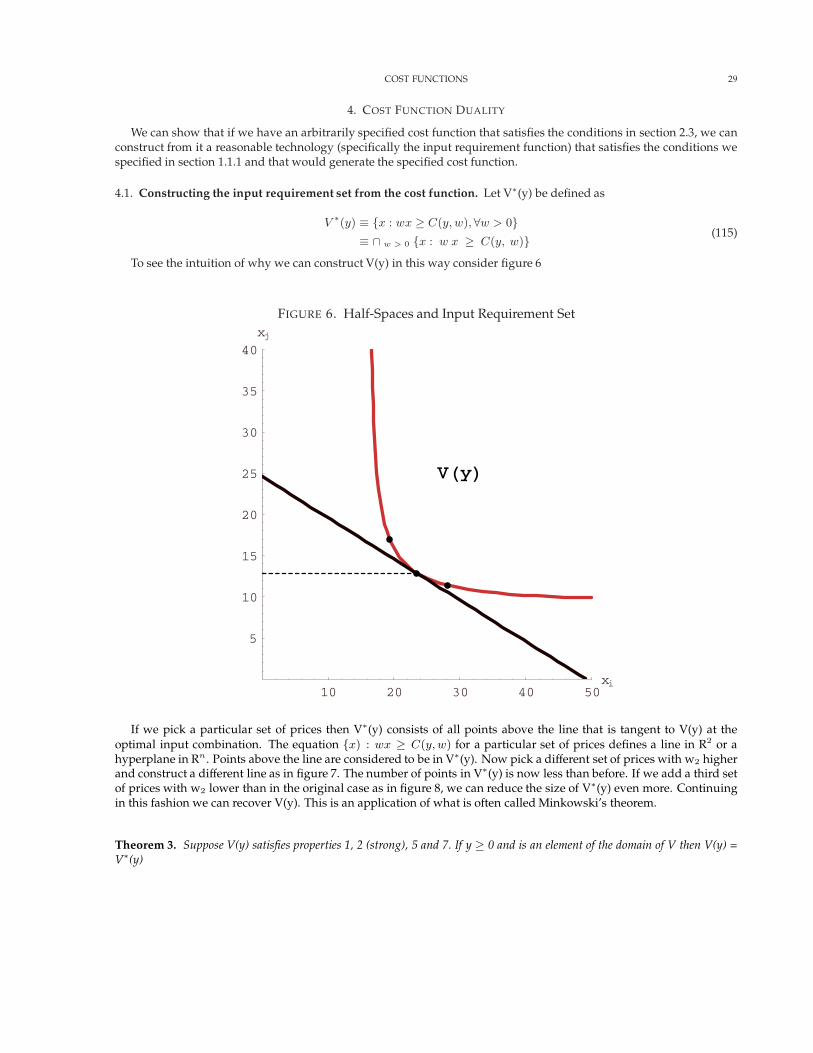
4.1. Constructing the input requirement set from the cost function. Let V∗(y) be defined as
V ∗(y) ≡ {x : wx ≥ C(y,w),∀w > 0}≡ ∩ w > 0 {x : w x ≥ C(y, w)}
(115)
To see the intuition of why we can construct V(y) in this way consider figure 6
FIGURE 6. Half-Spaces and Input Requirement Set
10 20 30 40 50xi
5
10
15
20
25
30
35
40xj
VHyL
If we pick a particular set of prices then V∗(y) consists of all points above the line that is tangent to V(y) at theoptimal input combination. The equation {x) : wx ≥ C(y,w) for a particular set of prices defines a line in R2 or ahyperplane in Rn . Points above the line are considered to be in V∗(y). Now pick a different set of prices with w2 higherand construct a different line as in figure 7. The number of points in V∗(y) is now less than before. If we add a third setof prices with w2 lower than in the original case as in figure 8, we can reduce the size of V∗(y) even more. Continuingin this fashion we can recover V(y). This is an application of what is often called Minkowski’s theorem.
Theorem 3. Suppose V(y) satisfies properties 1, 2 (strong), 5 and 7. If y ≥ 0 and is an element of the domain of V then V(y) =V∗(y)