cost-effective integration of efficient low-lift base … · cost-effective integration of...

PNNL-17157

*Visiting Professor Massachusetts Institute of Technology

Cost-Effective Integration of Efficient Low-Lift Base-Load Cooling Equipment - Final W. Jiang D.W. Winiarski S. Katipamula P.R. Armstrong* December 2007 Prepared for the U.S. Department of Energy Office of Energy Efficiency and Renewable Energy Federal Energy Management Program under Contract DE-AC06-76RL01830

DISCLAIMER This report was prepared as an account of work sponsored by an agency of the United States Government. Neither the United States Government nor any agency thereof, nor Battelle Memorial Institute, nor any of their employees, makes any warranty, express or implied, or assumes any legal liability or responsibility for the accuracy, completeness, or usefulness of any information, apparatus, product, or process disclosed, or represents that its use would not infringe privately owned rights. Reference herein to any specific commercial product, process, or service by trade name, trademark, manufacturer, or otherwise does not necessarily constitute or imply its endorsement, recommendation, or favoring by the United States Government or any agency thereof, or Battelle Memorial Institute. The views and opinions of authors expressed herein do not necessarily state or reflect those of the United States Government or any agency thereof.

PACIFIC NORTHWEST NATIONAL LABORATORY operated by BATTELLE

for the UNITED STATES DEPARTMENT OF ENERGY

under Contract DE-AC06-76RL01830

Printed in the United States of America

Available to DOE and DOE contractors from the Office of Scientific and Technical Information,

P.O. Box 62, Oak Ridge, TN 37831-0062; ph: (865) 576-8401 fax: (865) 576-5728

email: [email protected]

Available to the public from the National Technical Information Service, U.S. Department of Commerce, 5285 Port Royal Rd., Springfield, VA 22161

ph: (800) 553-6847 fax: (703) 605-6900

email: [email protected] online ordering: http://www.ntis.gov/ordering.htm

This document was printed on recycled paper. (8/00)

ii

Cost-Effective Integration of Efficient Low-Lift Base-Load Cooling Equipment - Final W. Jiang D.W. Winiarski S. Katipamula P.R. Armstrong* December 2007 Prepared for the U.S. Department of Energy Office of Energy Efficiency and Renewable Energy Federal Energy Management Program under Contract DE-AC06-76RL01830 Pacific Northwest National Laboratory Richland, Washington 99352

iii

Executive Summary The long-term goal of Department of Energy’s (DOE’s) Commercial Buildings Integration program is to develop cost-effective technologies and building practices that will enable the design and construction of net Zero Energy Buildings — commercial buildings that produce as much energy as they use on an annual basis — by 2025.1 To support this long-term goal, DOE further called for — as part of its FY07 Statement of Needs — the development by 2010 of “five cost-effective design technology option sets using highly efficient component technologies, integrated controls, improved construction practices, streamlined commissioning, maintenance and operating procedures that will make new and existing commercial buildings durable, healthy and safe for occupants.”2 In response, Pacific Northwest National Laboratory (PNNL) proposed and DOE funded a scoping study investigation of one such technology option set (TOS), low-lift cooling that offers potentially exemplary heating, ventilation and air conditioning (HVAC) energy performance relative to American Society of Heating, Refrigeration and Air Conditioning Engineers (ASHRAE) Standard 90.1-2004. The primary purpose of the scoping study was to estimate the national technical energy savings potential of this TOS. The TOS PNNL evaluated consists of:

1. Peak-load shifting by means of active or passive thermal energy storage (TES)3. 2. Dedicated outdoor air supply with enthalpy heat recovery from exhaust air. 3. Radiant heating and cooling panels or floor system. 4. Low-lift vapor compression cooling equipment. 5. Advanced controls at the HVAC equipment and HVAC system (supervisory) levels.

The application of the TOS was simulated in three medium-sized office building prototypes (baseline, mid-performance and high-performance, which are defined later in the report) in five climate zones around the U.S. Results from our analysis indicate that the technical HVAC energy savings potential of the TOS ranges from 60% to 74% for temperate to hot and humid climates, and 30% to 70% in milder climates. The savings are calculated as a difference between the annual energy use (chiller, fans and pumps) for a building with a conventional HVAC system and the annual energy use for the same building with equipment and controls of the TOS. Because of the nature of this scoping study, a number of assumptions had to be made. These assumptions are listed in the individual sections of the report, where appropriate, and collected for convenient reference in Appendix C. The national technical energy savings potential (cooling, fans and pumps) from the TOS were then estimated by scaling the savings from the prototype building. Table E-1 summarizes the national technical energy savings for the full TOS, compared to the conventional variable air volume (VAV) system with a two-speed chiller. Note that these estimates are for new construction and building-types and climate locations for which the full TOS is applicable. Although we think that parts of the TOS are applicable for a large portion of the existing 1 Fiscal Year 2007 Budget-in-Brief 2 Fiscal Year 2007 Commercial Buildings “Statement of Needs.” 3 In this report active denotes peak-shifting by means of a discrete TES such as a stratified water tank; passive refers to pre-cooling of the intrinsic mass (building fabric and contents) by forced air or hydronic radiant cooling using a chiller and/or air-, water-, or refrigerant-side free cooling.

iv

commercial building stock and the full TOS may be applicable to a fraction of the existing building stock, we did not estimate that potential in this study, because the primary market – as with most advanced TOS involving systems engineering in building design – is new construction. In this sense, the technical potential we present here is conservative. In addition, the savings estimates are for cooling systems (chiller, fan and pumps) only. If the heating systems savings were to be included, the estimates of energy savings would be higher still because the radiant cooling panel/dedicated outdoor-air system provides ventilation heat recovery, lowers air temperatures in the heating mode, and eliminates reheat energy and associated cooling load in zones that use reheat. For baseline buildings that are compliant with ASHRAE 90.1-2004, the full TOS saves about 0.010 quads of site electricity use in one year of new construction with the full TOS being applied to approximately 69% of floor area4 of total 2007 U.S. new commercial building stock; the annual site electricity savings are about 0.005 quads for mid-performance buildings and 0.003 quads for high-performance buildings. Assuming the new construction growth rates remain the same for the next 14 years (through the year 2020), the total national technical site energy savings potential (again assuming 100% penetration) for the baseline building would be 0.146 quads in 2020. To reiterate, all of these savings are in site energy terms; to calculate source energy savings at the power plant, using average fossil-steam heat rates, the previous estimates should be multiplied by 3.5 The total savings potential – relative to the baseline building – is therefore 0.44 quads in 2020.6

Table E-1 Summary of National Technical Site Energy Savings Potential for the Years 2007 and 2020 for the Low-Lift Cooling Technology Option Set (assuming 100% Penetration in

one year’s new construction for 2007 and 14 years’ new construction for 2020) National Cooling and Fan and Pump Energy Site

Electricity Savings (Quads) Building Performance Level 2007 2020

Baseline Building 0.010 0.146

Mid-Performance Building 0.005 0.072

High-Performance Building 0.003 0.042

4 assuming 100% penetration in that 69% of total floor area 5 Per the 2007 Buildings Energy Databook, the stock average fossil fuel steam heat rate (Btu/kWh) will be 10,181 in 2020 – see Table 6.2.5 http://buildingsdatabook.eren.doe.gov/docs/6.2.5.pdf This compares to the electricity consumption heat rate of 3412 Btu/kWh, about a factor of three difference. 6 For reference, one quadrillion Btu is equivalent to the output of 47 gigawatts of coal-fired capacity at current heat rates and capacity factors. See Table 6.1.2 http://buildingsdatabook.eren.doe.gov/docs/6.1.2.pdf

v

Table of Contents Executive Summary ....................................................................................................................... iii Acronyms and Abbreviations ........................................................................................................ ix Introduction..................................................................................................................................... 1 Background..................................................................................................................................... 2 Task 0: Literature Review............................................................................................................... 5

Summary of Literature Review................................................................................................... 6 Task 1: Produce Baseline Cooling Load Shapes ............................................................................ 8 Task 2: Baseline and Night Cooling Load Shapes........................................................................ 10

Optimal Chiller Dispatch with Ideal Storage............................................................................ 11 Standard and Peak-Shifted Chiller Annual Load Distributions................................................ 12

Task 3: Develop Component Models ........................................................................................... 16 Task 4: National Technical Energy Savings Potential.................................................................. 18

Energy Use Estimates for the Various TOS and Building Configurations............................... 20 National Energy Savings Estimation Methodology.................................................................. 25

Climate Zone Mapping ......................................................................................................... 26 Building Type Mapping........................................................................................................ 30

National Energy Savings Estimation ........................................................................................ 31 Acknowledgement ........................................................................................................................ 33 References..................................................................................................................................... 34 Appendix A. Literature Review.................................................................................................... 36

High Performance Buildings (HPB) and Associated Technologies ......................................... 39 Discrete Cool Storage ............................................................................................................... 40 Cooling load peak shifting controls .......................................................................................... 41 Zone Thermal Response Models and Model Order Reduction ................................................ 43 Inverse Models.......................................................................................................................... 44 Load Forecast-Based Controls.................................................................................................. 45 Vapor-Compression Cycle Efficiencies and Advanced Package A/C...................................... 46 Compressor and Equipment Ratings and Performance Maps................................................... 48 Enthalpy Recovery and DOAS ................................................................................................. 50 Cooling by Radiant Panels........................................................................................................ 51 Radiant Cooling Integration with DOAS.................................................................................. 52 Radiant Cooling and Chiller or Heat Pump COP ..................................................................... 54 Active Core Cooling ................................................................................................................. 54 Low Fan Power and Displacement Ventilation ........................................................................ 56 Static Chiller Optimization ....................................................................................................... 56 Technical Potential and Market Assessments........................................................................... 58

Appendix B. TOS Component Models......................................................................................... 60 Appendix B. TOS Component Models..................................................................................... 61 Optimal Chiller Performance Model ........................................................................................ 61 Compressor Model.................................................................................................................... 61 Evaporator Model ..................................................................................................................... 65 Condenser Model ...................................................................................................................... 65 Transport (fan and pump) Power Model................................................................................... 65 Radiant Cooling Panel Model................................................................................................... 66 Fan-Coil Model for CV or VAV Distribution .......................................................................... 68

vi

Optimal Chiller Performance Map............................................................................................ 70 Hourly Cycling Performance of Two-Speed Chillers............................................................... 74 Hourly Cycling Performance of Two-Speed Chiller in Unoccupied Hours ............................. 75 Refrigerant-side Economizer (Free Cooling) Model ................................................................ 76 Dedicated Outdoor Air System (DOAS) DX-Dehumidifier Model ......................................... 78

Derivation of DX Coil Model ............................................................................................... 81 Appendix B References ............................................................................................................ 85

Appendix C. Modeling and Analysis Assumptions...................................................................... 86

vii

List of Figures Figure 1 - Three-Dimensional Models of the Small and Medium Office Prototypes .................... 8 Figure 2 - Example Building Sensible Load Shapes for Houston; Time Index Starts at End of

Occupancy (0 on the x-axis represents 6 p.m.) ..................................................................... 10 Figure 3 - Baseline Building Sensible Cooling Load Distribution for Chicago ........................... 13 Figure 4 - Building Peak-Shifted Cooling Load Distribution for Variable-Speed Chiller with

RCP/DOAS system for Chicago........................................................................................... 13 Figure 5 - Results of Baseline Building Annual Energy Simulations for Different Chiller-

Distribution System Configurations in Five Climates .......................................................... 20 Figure 6 - Results of Mid-Performance Building Annual Energy Simulations for Different

Chiller-Distribution System Configurations in Five Climates.............................................. 21 Figure 7 - Results of High-Performance Building Annual Energy Simulations for Different

Chiller-Distribution System Configurations in Five Climates.............................................. 22 Figure 8 - Mapping between NREL Climate Zones and Low-Lift Climate Zones (bolded climate

zones were not included) ...................................................................................................... 26 Figure 9 - National Technical Site Electricity Savings over the Conventional VAV System with

2-speed Chiller (case 1) for Different System Configurations for the Year 2007 Assuming 100% Penetration in One Year’s New Construction. ........................................................... 32

Figure 10 - National Technical Site Electricity Savings in 2020 over the Conventional VAV System with two-speed Chiller (Case 1) for Different System Configurations for 2020 Assuming 100% Penetration over Fourteen Years of New Construction............................. 33

viii

List of Tables Table 1 - Analysis Grid for Simulating Baseline Cooling Load Profiles ....................................... 9 Table 2 - Annual FLEOHs by Part-Load Ratio (across) and Outdoor Dry-Bulb Temperature

(down) for Baseline for Chicago........................................................................................... 14 Table 3 - Annual FLEOHs by Part-Load Ratio (across) and Outdoor Dry-Bulb Temperature

(down) for Variable-Speed Chiller with RCP/DOAS for Chicago....................................... 15 Table 4 - Analysis Grid of Non-HVAC Building Design Performance Characteristics ............... 19 Table 5 - Annual Chiller, Pump and Fan Energy Use (kWh) for the eight TOS Configurations

and three Medium-Office Building Configurations.............................................................. 23 Table 6 - Percent Energy Savings (Chiller, Pump and Fan) for the seven TOS and three Medium-

Office Building Configurations Compared to Base Case (Case 1)....................................... 24 Table 7 - Benchmark Building Prototype Areas (Long 2007)...................................................... 25 Table 8 - Number of New Buildings Built Each Year by Type in each Climate Zone (Long 2007)

............................................................................................................................................... 27 Table 9 - New Building Floor Area (sf) built each year by Type for Zones 1, 2 and 3................ 28 Table 10 - New Building Floor Area (sf) built Each Year by Type for Zone 4 through 8........... 29 Table 11 - Building Types Included in National Energy Savings Analysis ................................. 30 Table 12 - Summary of National Technical Site Electricity Savings Potential for the Year 2007

for the Low-Lift Cooling Technology Option Set (assuming 100% Penetration)................ 31 Table 13 - Summary of Total National Technical Site Electricity Savings Potential in 2020 for

the Low-Lift Cooling TOS (assuming 100% Penetration) ................................................... 32

ix

Acronyms and Abbreviations A/C air conditioning AEDG Advanced Energy Design Guide AHU air handler unit ANSI American National Standards Institute ARI American Refrigeration Institute ARTI Air-Conditioning and Refrigeration Technology Institute ASHRAE American Society of Heating, Refrigeration and Air-Conditioning Engineers BT Building Technologies Program CBECS Commercial Building Energy Consumption Survey CFC chlorofluorocarbons cfm cubic feet per minute COP coefficient of performance CV constant volume air distribution system CRTF comprehensive room transfer function CTF conduction transfer function DCV demand-controlled ventilation DDC direct digital control DOAS dedicated outdoor air conditioning system DOE U.S. Department of Energy DV displacement ventilation DX direct expansion ECM electrically commutated motors EER energy efficiency ratio EIA Energy Information Administration ERV energy recovery ventilation EUI energy use intensity FLEOH full-load-equivalent operating hours FDD fault detection and diagnostics GIS geographical information systems GSA General Services Administration HP heat pump HPB high-performance building HX heat exchanger HSTF heat source transfer function HVAC heating, ventilation and air conditioning IAQ indoor air quality IESNA Illuminating Engineering Society of North America kBh thousand Btu per hour kWh kilowatt hours LBNL Lawrence Berkeley National Laboratory NZEB Net-Zero Energy Building NREL National Renewable Energy Laboratory PCM phase change materials PNNL Pacific Northwest National Laboratory PLR part load ratio QUAD quadrillion (1015) British Thermal Units (Btus) R&D research and development

x

RCP radiant cooling panel RTP real-time pricing (electric utility rate) SEER seasonal energy efficiency ratio SHGC solar heat gain coefficient SHR sensible heat ratio SP special projects (working groups within ASHRAE) TES thermal energy storage TOS technology option set TOU time of use (utility rate) UA conductance coefficient UFAD under-floor air distribution VAV variable air volume VRV variable volume refrigeration VSD variable speed drive w/cfm Watts per cubic feet per minute (measure of fan power efficiency) W/sf Watts per square foot WWR window-to-wall Ratio ZEB zero energy building

1

Introduction This report describes the work performed in FY07 on the technology option set (TOS) entitled, “Cost-Effective Integration of Efficient Low-Lift Base Load Cooling Equipment.” The technical approach and results are reported for work completed in each of five tasks - Task 0 (Literature Review), Task 1 (Develop Baseline Cooling Load Shapes), Task 2 (Develop Technology Option Set Cooling Load Shapes), Task 3 (Develop Component Models) and Task 4 (National Technical Energy Savings Potential Preliminary Results). In January 2007, under Task 0, Pacific Northwest National Laboratory (PNNL) prepared and submitted a summary literature review for all technology options that are considered in this project (Appendix A). In July 2007, a mid-year letter report was submitted. The mid-year report provided the status of the project as of June 2007, and the main findings reported at mid-year are included in this report for completeness. In the course of the project, PNNL has developed the initial design of chillers specifically intended for operation with sensible load peak-shifting controls and of separate efficient latent cooling subsystems. Preliminary results from the current analysis indicate technical chiller, fan and pump energy savings potential from use of the proposed TOS range from 60% to 74% for temperate to hot and humid climates and 30% to 70% in milder climates with high economizer and night free-cooling potential. The savings are calculated as a difference between the annual energy use (chiller, fan and pump) for a building with conventional heating, ventilating, and air conditioning (HVAC) system and the annual energy use for the same building with the TOS. Note that because of the nature of this scoping study, a number of assumptions had to be made. These assumptions are listed in the individual sections of the report, where appropriate, and collected for convenient reference in Appendix C.

2

Background Design of cost-effective high-performance buildings has focused mainly on lighting, window and other envelope measures. Efforts directed at HVAC performance have tended to pursue, and in many cases achieved, incremental efficiency improvements. These efforts, even when combined with radiant panel distribution or night pre-cooling concepts however, have continued to assume a more or less conventional cooling plant. Conversely, efforts to optimize chiller and thermal energy storage (TES) operations have generally assumed a conventional air-distribution system. The thrust of this TOS is to significantly reduce HVAC energy consumption through utilization of synergies between emerging HVAC technologies and advanced controls. This approach seeks to improve the part-load efficiencies of equipment and the operational efficiency of the building as an integrated system. The technology option set consists of:

1. Peak-load shifting by means of active or passive (pre-cooling of building mass) TES. 2. Dedicated outdoor air system (DOAS) and enthalpy heat recovery from exhaust air. 3. Radiant heating and cooling panels or floor system. 4. Low-lift7 vapor compression cooling equipment. 5. Advanced controls at the HVAC equipment and HVAC system (supervisory) levels.

Although these technologies can and have been used independently to provide incremental savings, when used together, they achieve significant energy savings by integrating HVAC equipment, distribution and control in a highly synergistic manner. Peak shifting and active and passive thermal energy storage are proven technologies that improve chiller load factor and can increase chiller efficiency. DOAS with enthalpy recovery8 provide more efficient latent cooling so that radiant cooling can be used to satisfy sensible cooling loads. Radiant cooling further increases chiller efficiency by allowing the temperature of the radiant panel/ceiling, and hence of the chilled water supplied, to be only a few degrees below room temperature. Compared to all-air systems, the fan energy use of a radiant cooling panel (RCP)/dedicated outdoor air system is dramatically reduced. If water is used as a transport medium for heating and cooling, it can actually be used as short-term thermal storage to alleviate temporary peak demands. When advanced controls are integrated with the above technologies, additional energy and peak demand savings can be achieved by coordinating variable-speed compressors, fans and pumps for maximum efficiency, by anticipating and shifting daytime cooling loads, and by eliminating simultaneous heating and cooling. It is recognized that substantial efficiency improvements in office, retail and other building types can be achieved with advanced envelopes (e.g. reduced conduction and infiltration, improved windows), lighting technologies/controls, and plug load power density reductions. These technologies are basic to continued advances in overall energy efficiency. As the envelope

7The American Refrigeration Institute defines chiller part-load rating conditions as 50oF chilled water supply and 80oF outdoor dry-bulb temperature; we consider low-lift conditions to be 60-65oF chilled water supply, ~80oF outdoor dry-bulb temperature (day) and ~70oF outdoor dry-bulb temperature (night). 8Uses outdoor-exhaust air enthalpy difference to pre-heat and humidify or pre-cool and pre-dry outdoor air..

3

reaches a very high level of performance and ventilation load is taken up by a DOAS, the remaining cooling load will be dominated by internal gains: lights, plugs, and people. Most building types will have—and all building core zones have always had—cooling load patterns that do not vary much from week to week and even from summer to winter seasons. This is the ideal situation for a baseload cooling system with modest storage—analogous to a light, streamlined hybrid vehicle with a small and very efficient engine. With the assumed low design load (high performance envelope and low lighting and equipment power densities) for cooling loads that can be satisfied with higher chilled water and supply air temperatures (60 to 65oF) and, with roughly half of the cooling delivered at night, the lowest life-cycle-cost plant will be one that is optimized for low condensing temperature (75oF or less) as well. Hydronic radiant cooling distribution can only be used in conjunction with DOAS equip-ment to address latent load. One can thus consider a TOS to address the cooling and ventilation piece of the zero energy building (ZEB) puzzle as an integration of three key elements:

1. Efficient low-lift (75oF condenser, 60oF evaporator) variable-speed cooling plant. 2. Intrinsic building mass and controls to halve the typical cooling plant load factor. 3. RCP/DOAS with enthalpy recovery and efficient distribution

One of the main impediments to significant increases in cooling plant efficiency is cost. It is difficult to justify costs of increased heat transfer area; larger, slower turning compressors; and less restrictive piping when the duty-cycle is rarely more than 20% and often less than 10% on an annual basis (8,670 hours). Efficient pre-cooling of building mass, enabled by advanced controls and efficient distribution, has two potential effects on chiller cost and performance: 1) the plant operates at much lower average discharge pressure, and 2) shifting load away from the peak can reduce the required cooling plant capacity. Other high performance building characteristics involving the envelope, windows and shading, lighting and controls, and office equipment can be expected to reduce peak cooling loads by at least 50%. With the reduction in plant capacity, further improvements in chiller plant efficiency can be justified. These improvements may include:

• Reduced flow losses by reducing compressor speed and increasing free area of valves; • Compressor design optimized for low compression ratio; • Reduced heating of refrigerant vapor as it enters the compressor; • Refrigerant mixture to reduce pressure difference between evaporator and condenser; • Use of higher efficiency compressor motor and inverter; • Rejecting compressor motor heat directly to ambient air or cooling tower water; • Large heat transfer areas and low flow losses on refrigerant side of evaporator and

condenser; • Large heat transfer areas and low flow losses on load side of evaporator and heat-

rejection side of condenser; • Use of flooded-evaporator design to achieve very low superheat and high suction density; • Modulation of load- and heat-rejection-side flow rates to reduce transport energy; • Low restriction oil separator or use of oilless compressor design.

4

The theoretical potential for high efficiency, low-lift vapor-compression cooling is well understood. The source and sink temperatures between which a thermodynamic cycle operates are determined by conditions and by approach temperatures in the load-side and rejection-side heat exchangers. The Carnot and Lorentz ideal cycle efficiencies represent fundamental upper bounds on performance to which current products and standards do not come anywhere near. Industry has argued that further improvements are not cost effective. However the value engineering analyses that reach these conclusions typically assume current design practices such as not using thermal storage, using the same heat exchanger for sensible and latent cooling, using fixed-speed motors and sizing for peak load. Most cool storage installations to date have been justified by time-of-use electric rates; none have, to our knowledge, used chillers optimized for low-lift operation or for very efficient operation at less than half rated capacity. The main reasons for this are: 1) the double approach temperature penalty inherent in most discrete cool storage configurations, 2) a dearth of low-lift, high part-load efficiency chillers in the marketplace, and 3) low probability of finding an owner willing to try two or three new, mutually dependent cooling technologies in the same building. The proposed TOS is applicable to most commercial building types and climates where mechan-ical cooling equipment is considered necessary (cooling applications that cannot be 100% satisfied by natural ventilation or air- or water-side economizer operation). This market represents well over half of the entire U.S. commercial building sector even if we count only applications that benefit from all elements of the TOS. However, the scoping study has focused on the analysis of the single most common building type and footprint – a medium office building – with three different energy performance levels. Implementations of various combinations of TOS elements are analyzed to understand the interactions. Each combination of TOS elements, as well as the baseline equipment configuration, is analyzed at each building performance level and in each of five climate zones.

5

Task 0: Literature Review A detailed literature review was conducted to document past applications experience and the current state-of-art of advanced technologies and controls relevant to the TOS. The results of this task, completed in January 2007, have guided work throughout the project. The full literature review is reproduced in Appendix A. The previous work most directly relevant to the low-lift cooling TOS modeling and assessment activities may be summarized as follows. Night pre-cooling has been successfully demonstrated in a few large (>100,000 sf) buildings in which high cooling and distribution efficiencies under low-ambient part-load conditions are exhibited. Results of night pre-cooling have been less successful in small buildings, where constant volume night fan operation is a significant penalty (relative to a large building, where fan speed and static pressure can typically be adjusted by the control system) and existing typical direct expansion (DX) package equipment efficiency does not improve much as ambient temperature drops. The potential for closing the performance gap between small- and large-capacity cooling equipment, together with the continually falling costs of microprocessor-based package-unit controls and high efficiency variable speed motors and drives, present a strong motivation to develop low-lift package cooling equipment technologies for mild climates and climates with cool nights. With active core cooling and dedicated outdoor air-conditioning (A/C) systems (DOAS), the energy benefits can be extended to hot and humid climates as well. Refrigerant-side free-cooling has been mentioned, but details of design and performance were not found in the literature, probably because this design traditionally has had little attraction when used with 1) the low chilled-water temperatures required for conventional air-handling unit (AHU) and fan-coil latent-plus sensible-cooling distribution systems, 2) systems that use ice storage9, or 3) systems with cooling towers. The energy savings and market application potentials for the refrigerant-side economizer option in buildings with radiant cooling and small air-cooled chiller plants should be explored. The DOE Commercial Unitary Air Conditioner report (2004) found that the best path for getting DX package equipment efficiency improvements from EER-10 to EER-12 was to increase evaporator and condenser size. The question of how to best improve annual performance—e.g. with the higher chilled water temperatures associated with radiant panel (or radiant slab) systems and for the probability distribution of outdoor conditions experienced with peak shifting controls—will have to be addressed further. There appear to be no studies of national energy savings potential, even for buildings with chillers that would provide good low-lift performance. Recent work by proponents of radiant cooling has focused on accurately estimating panel capacity, on modeling the interactions of convection and radiation, and on supervisory control strategies of decoupled dehumidification/ventilation and sensible cooling systems that ensure comfort and acceptable indoor air quality (IAQ) while avoiding condensation on panels under all conditions. One paper estimates fan energy and higher-air-temperature-effected savings. The

9For warmer storage, a refrigerant-side economizer is feasible but not as efficient as the “filter cycle”.

6

loss of 80% of the normal air-side free cooling potential has been noted, but the potential national impact of this loss has not been addressed. The effectiveness and national potential of applying water- and refrigerant-side economizers in conjunction with radiant cooling have not been evaluated. The potential system efficiency improvements of active core cooling combined with peak-shifting and efficient low-lift chiller equipment have not been quantitatively assessed. Work on active core cooling has addressed thermal occupancy conditions such as strong vertical temperature gradients. The considerable challenge of control during diurnal and shorter load transients seems to need more work. The potential system efficiency improvements of active core cooling, combined with peak-shifting and efficient low-lift chiller equipment, have not been assessed. Work on DOAS has focused on proper control over the wide range of outdoor conditions that such systems face, and on performance-cost-pressure drop considerations—trade-offs to which package A/C plants are particularly sensitive. Mention of design integration problems is conspicuously absent from the literature, as one might expect, because DOAS has been treated as providing a predominantly stand-alone function. The literature does not mention cascading of a dehumidifying DX machine to the main chiller or storage tank. Supervisory control of reheat (and determination of the optimal DOAS supply air temperature) is another area of interaction with the radiant cooling that may need further study. The proposed package chiller solutions achieve high annual performance by increasing evaporator and condenser size, by use of a liquid receiver at the condenser outlet and a flooded evaporator, and by optimal control of compressor, fan and pump speeds for any given condition. The most familiar comprehensive work on coordinating compressor, fan and pump speeds, sometimes referred to as “optimal static chiller control,” is that of Braun et. al. (1987a,b; 1989a,b,c; 1990). Static chiller optimization has been applied to large plants both with and without discrete cool storage. The technical potential of combining radiant cooling with small variable speed drive (VSD) package chillers optimized for low-lift conditions has not been addressed. There do not appear to be any economic analyses of small package low-lift equipment or small package DOAS conditioning equipment. It is difficult to predict what such equipment would cost in a commodity market—or even in substantial niche markets—because it is not currently produced in any standard product line.

Summary of Literature Review In summary, a careful review of the literature reveals a great deal of effort and progress toward characterizing, developing, and demonstrating individual efficient cooling technologies. However three major gaps exist:

1) There is a need to examine multiple efficient cooling technologies—especially technologies that appear to be highly complementary—by system-level simulations to determine which combinations work best in various building designs and climates.

7

2) The national potential of deploying the most promising combination(s) needs to be assessed based on the simulation results.

3) Performance of well-designed and commissioned TOS configurations needs to be demonstrated for a range of climates in buildings that are state-of-the-art in terms lighting, envelope, and efficient office equipment, and reasonably generic in terms of occupancy and use.

8

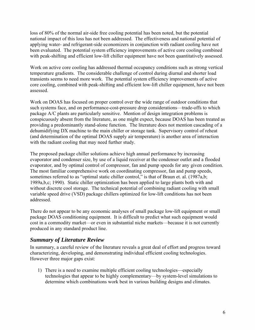
Task 1: Produce Baseline Cooling Load Shapes The objective of Task 1 was to explore the range of cooling load shapes in commercial buildings resulting from different levels of balance-of-system cooling load reduction measures and night pre-cooling capacity. The load shapes developed in this task are used in the next task (Task 2) to determine how peak-shifting impacts the part-load load distribution which, in turn, affects low-lift chiller design. Two sets of baseline office building prototypes were reviewed for the current work – the Lawrence Berkeley National Laboratory’s (LBNL’s) prototypes (Huang and Franconi, 1999) and the Advanced Energy Design Guide (AEDG) small office prototypes (Jarnagin, et al., 2006). The prototypes for AEDG were selected for this analysis because the DOE-2 building models had been extensively vetted within the ASHRAE Special Projects working group (SP102) and provided building descriptions with configuration and energy performance features typical of new construction. The SP102 working group developed two baseline office building prototypes (5,000 ft2 frame building and 20,000 ft2 two-story building) for the AEDG work, as shown in Figure 1. The baseline AEDG prototypes are in compliance with ASHRAE Standard 90.1-2001 and ANSI/ASHRAE/IESNA10 Standard 90.1-1999, Energy Standard for Building Except Low-Rise Residential Buildings. The 5,000 ft2 building, which is referred to as a small office, is a single thermal zone building served by one single-zone packaged rooftop unit. The 20,000 ft2 building, which is referred to as a medium office, consists of five thermal zones with each zone served by a packaged rooftop unit.

Figure 1 - Three-Dimensional Models of the Small and Medium Office Prototypes

In Task 1, the AEDG prototypes were updated to comply with Standard 90.1-2004 and specifi-cation of an “analysis grid,” keyed to this baseline, was completed (Table 1). Three component performance levels were enumerated in each of the following analysis grid dimensions:

• Wall and roof U-factor, • Window performance [U-factor and solar heat gain coefficient (SHGC)], • Window-wall ratio and shading, • Light and plug load power density, • Fan power.

10 ANSI – American National Standards Institute; ASHRAE – American Society of Heating, Refriger-ation and Air Conditioning Engineers; IESNA – Illuminating Engineering Society of North America.

9

Table 1 - Analysis Grid for Simulating Baseline Cooling Load Profiles Component Performance Levels to be Analyzed

Component Baseline Mid-Performance High Performance Wall-Roof U-Factor 90.1-2004(a) 2/3 of 90.1-2004 4/9 of 90.1-2004 Window U-Factor and SHGC 90.1-2004(a) 2/3 of 90.1-2004 4/9 of 90.1-2004 Window-to-Wall-Ratio 40% 20% 20%+Shading(b) Light and Plug Loads(c) (W/sf) 1.3+0.63 0.87+0.42 0.58+0.21 Fan Power (W/scfm)(d) 0.8 0.533 0.356

(a) Because the values vary by climate zones, the values are not listed in this table (b) Completely shade the solar direct beam (c) Power density during hours of the highest loads defined in the DOE-2.2 weekly load schedules (d) Total HVAC fan power divided by total HVAC fan flow rate

The limited scope of the present study dictated that only one building footprint be analyzed. The medium office prototype was simulated using DOE-2.2 to produce cooling load distributions for all points on the analysis grid at five representative climate zones. The total number of baseline building cooling load distributions produced by simulation was 3x3x3x3x3x5 = 1215. Because of the longer computation times, only the Baseline, Mid- and High-Performance buildings were simulated with peak shifting resulting in 3x5=15 combinations of building and climate for the final savings analysis. The selected five representative climate locations are Baltimore, Chicago, Houston, Los Angeles and Memphis. We considered these climates as representative of the five key climate zones used by the Department of Energy (DOE) in its building energy codes development work (Briggs et. al., 2002), and together the five DOE climate zones encompass about three-fourths of the U.S. population. These climate zones capture significant variability of both outside-air temperature and humidity, and of day length and sun-sky conditions. Chicago (N41.8°) has cold and dry winters and represents the single most populous climate zone. Los Angeles (N33.9°) is warm and dry during most of the year and represents the southwestern U.S. maritime region. Memphis (N35.1°) and Baltimore (N39.2°) have mild weather and represent the middle latitudes of the U.S. Houston (N30.0°) represents the hot and humid climates found along the U.S. Gulf Coast.

10

Task 2: Baseline and Night Cooling Load Shapes The technology option set (TOS) being evaluated in this study can shift a significant portion of the sensible cooling load to night-time hours. To estimate the national potential energy savings from the TOS, we not only need a baseline load shape but also a load shape that is flattened by shifting part of the load to nighttime hours. The benefit of shifting some or the entire chiller load into night-time hours is to present to the chiller a total cooling load equal to the base building design load, but under the low-lift conditions, provided by operation at a lower part-load fraction and/or by operation at cooler night and early morning temperatures. This is in stark contrast to the traditional chiller or package A/C operation, where cooling loads are concentrated around times of peak outdoor-air temperature. Figure 2 shows typical sensible cooling load shapes for the prototypical small office building in Houston. Compared to the baseline load shape for a typical packaged single zone system (“bas”), the optimally peak-shifted load shape for a variable speed chiller and radiant panel cooling system (“pvr”) is flattened by shifting part of the daytime cooling load to nighttime.

0 4 8 12 16 20 240

10

20

30

40

50

60

70

hour

build

ing

dens

ible

coo

ling

load

(kB

tu)

Houston

baspvr

Figure 2 - Example Building Sensible Load Shapes for Houston; Time Index Starts at End of Occupancy (0 on the x-axis represents 6 p.m.)

A cool storage device or subsystem and a load-shifting algorithm are required to implement the peak-shifting element of the TOS. The peak-shifting element is introduced early in our work (as Task 2) to provide an annual distribution of chiller load as a function of outdoor conditions and part-load ratio. This load distribution provides most of the information needed to assess chiller design and performance when night cooling is used to promote efficient part-load operation with variable-speed compressors, fans and pumps. The load distribution and chiller performance map (Task 3) together provide an estimate of annual energy use. Estimates of annual energy use for a prototypical building with baseline HVAC equipment and with that baseline equipment replaced by the TOS are used in the assessment of national energy savings potential, Task 4.

11

For this effort (FY07), we have presumed an idealized TES in order to quickly estimate the potential energy impact of load shifting. The idealized TES is equivalent to a lossless and perfectly stratified chilled water storage. However, a 24-hour carryover constraint is also assumed. Not admitting carryover has two important effects:

1) the storage capacity actually used can never exceed the peak daily cooling load and

2) performance of a building with real TES can approach that of a building with a zero-loss, perfectly-stratified TES that is never used to store more than the next day’s cooling .

We will henceforth use the phrase ideal TES to denote a lossless, perfectly stratified TES with zero diurnal carryover. The savings based on an ideal TES are felt to be reasonably close to the savings that can be achieved in the real world with passive (intrinsic mass) storage for cases where total daily load can be stored with acceptable room temperature excursions.

Optimal Chiller Dispatch with Ideal Storage A supervisory control strategy is required to find the peak-shifted cooling load trajectory that minimizes input energy given the baseline building cooling load trajectory and the performance characteristics of a chiller, some form of TES, and the associated mechanical (transport) equipment. If we assume storage with no losses and further assume no storage carryover from one day to the next and capacity sufficient for the peak cooling day, the problem is greatly simplified. Making use of the chiller performance model, as described in Task 3, we postulate a control that finds the sequence of 24-hourly chiller cooling rates Q(t), to minimize daily chiller input energy in the form of the following objective function:

Minimize ∑=

=24

1 )()(

t chiller ttQJ

η (eqn. 1)

subject to the daily load requirement:

∑∑==

=24

1

24

1)()(

ttLoad tQtQ

and to the capacity constraints: 0 ≤ Q(t) ≤ QCap(TX(t),TZ(t)) t = 1:24 where

ηchiller = f(TX,TZ,QLoad) = chiller efficiency (kBh/kW or ton/kW or kWth/kWe), TX = outdoor dry- or wet-bulb temperature, TZ = zone temperature, Q = evaporator heat rate—positive for cooling (kBh or ton or kWth), QLoad = building cooling load with no peak-shifting, and QCap = chiller cooling capacity.

The Q(t) constraint represents design variable upper and lower bounds in exactly the form needed to cast the problem as a bounded, but otherwise unconstrained, search—which is generally advantageous in terms of reliable convergence and computational efficiency.

12

MATLAB11 optimization function fmincon (find a minimum of a constrained nonlinear multivariable function) was used to find the hourly chiller cooling rates that minimize the daily chiller input energy. An initial search point that worked well for this application is the vector of uniform hourly average cooling rates based on the total daily load:

∑=

=24

1)(

241)(

tLoad tQtQ

Given an annual building cooling load profile and annual time series of outdoor dry-bulb temperature and zone temperature, one can run the optimization in 365 one-day blocks to find the hourly chiller cooling rates, which we will call the peak-shifted load profile, that minimizes the power input integrated over all 8,760 hours of the year. The standard and peak-shifted load profiles can then be parsed, by bin analysis, into bivariate distributions of cooling load versus part load fraction and outdoor dry-bulb temperature.

Standard and Peak-Shifted Chiller Annual Load Distributions Preliminary assessments of the TOS equipment configuration were made to compare the resulting annual chiller load distribution to the baseline load distribution. The baseline load distribution is fully determined by the building characteristics, defined in Task 1, and the climate. For Task 2, the full TOS configuration, consisting of a low-lift variable-speed chiller with RCP/DOAS and ideal TES, was simulated using the optimal chiller dispatch algorithm described above to produce a peak-shifted load profile for each climate that is then parsed into a peak-shifted load distribution.

Building cooling load profiles generated from Task1 were used as a baseline to compare to the peak-shifted cooling load profiles. Five baseline cooling load profiles for the medium-office building representing ASHRAE Standard 90.1-2004 building performance requirements at selected five climate zones are used in this preliminary assessment.

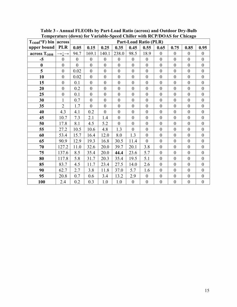
Figure 3 and Table 2 show the baseline cooling load distribution for the medium office at different temperature bins and part-load ratios for Chicago; Figure 4 and Table 3 show the optimally peak-shifted cooling load distribution for the medium office using a variable-speed chiller and RCP/DOAS system and idealized TES. The graphs illustrate the distribution of annual cooling load, expressed in full-load-equivalent operating hours (FLEOH), as a function of outdoor dry-bulb temperature and part-load ratio.

Compared to the baseline load distribution, the operation hours for the full TOS (variable-speed chiller, RCP/DOAS, TES) system are significantly shifted to lower part-load ratio in three respects. First, the bin in which the FLEOH peak occurs is typically 15°F lower than in the baseline chiller load distribution; second, although the chiller does continue to operate at high outdoor temperatures, it does so at much lower part-load ratios; and third, the FLEOHs of operation at low outdoor temperature and low part-load ratio are significantly increased.

11MATLAB is a high-level programming language and interactive environment used to develop and perform computational applications faster than with traditional programming languages such as C, C++, and Fortran.

13

0

0.5

1

0

50

100

0

10

20

30

40

50

part load ratio

Chicago---baseline

outdoor dry-bulb temperature (deg F)

FLE

OH

5

10

15

20

25

30

35

40

45

Figure 3 - Baseline Building Sensible Cooling Load Distribution for Chicago

0

0.5

1

0

50

100

0

10

20

30

40

50

part load ratio

Chicago---variable-speed chiller with RCP/DOAS

outdoor dry-bulb temperature (deg F)

FLE

OH

5

10

15

20

25

30

35

40

Figure 4 - Building Peak-Shifted Cooling Load Distribution for Variable-Speed Chiller

with RCP/DOAS system for Chicago

14

Table 2 - Annual FLEOHs by Part-Load Ratio (across) and Outdoor Dry-Bulb Temperature (down) for Baseline for Chicago

Part-Load Ratio (PLR) TODB(°F) bin upper bound

across PLR 0.05 0.15 0.25 0.35 0.45 0.55 0.65 0.75 0.85 0.95

Across TODB →↓→ 16.8 42.2 77.5 56.7 26.5 44.2 55.6 91.3 121.0 98.1 -5 0 0 0 0 0 0 0 0 0 0 0 0 0 0 0 0 0 0 0 0 0 0 0 5 0 0 0 0 0 0 0 0 0 0 0 10 0 0 0 0 0 0 0 0 0 0 0 15 0 0 0 0 0 0 0 0 0 0 0 20 0 0 0 0 0 0 0 0 0 0 0 25 0 0 0 0 0 0 0 0 0 0 0 30 0 0 0 0 0 0 0 0 0 0 0 35 0 0 0 0 0 0 0 0 0 0 0 40 0.3 0.3 0 0 0 0 0 0 0 0 0 45 0.5 0.3 0.3 0 0 0 0 0 0 0 0 50 8.6 0.7 3.6 2.0 2.2 0 0 0 0 0 0 55 13.6 0.6 5.1 6.0 2.0 0 0 0 0 0 0 60 19.2 1.1 3.8 7.2 7.1 0 0 0 0 0 0 65 6.1 1.4 1.1 2.6 0.9 0 0 0 0 0 0 70 26.0 4.2 7.7 10.0 3.3 0.8 0 0 0 0 0 75 68.5 0.4 1.3 5.7 19.9 20.2 15.3 5.8 0 0 0 80 139.4 5.0 5.9 2.7 1.8 4.6 22.1 29.9 40.9 22.9 3.7 85 155.7 2.9 10.1 22.5 3.1 0.9 6.8 13.2 32.4 40.5 23.3 90 134.8 0 3.3 17.5 8.5 0 0 6.7 14.4 36.0 48.4 95 51.9 0 0 1.1 5.4 0 0 0 3.64 19.9 21.8 100 5.4 0 0 0.3 2.5 0 0 0 0 1.7 0.9

15

Table 3 - Annual FLEOHs by Part-Load Ratio (across) and Outdoor Dry-Bulb Temperature (down) for Variable-Speed Chiller with RCP/DOAS for Chicago

Part-Load Ratio (PLR) TODB(°F) bin upper bound

across PLR 0.05 0.15 0.25 0.35 0.45 0.55 0.65 0.75 0.85 0.95

across TODB →↓→ 94.7 169.1 140.1 238.0 98.5 18.9 0 0 0 0 -5 0 0 0 0 0 0 0 0 0 0 0 0 0 0 0 0 0 0 0 0 0 0 0 5 0 0.02 0 0 0 0 0 0 0 0 0 10 0 0.02 0 0 0 0 0 0 0 0 0 15 0 0.1 0 0 0 0 0 0 0 0 0 20 0 0.2 0 0 0 0 0 0 0 0 0 25 0 0.1 0 0 0 0 0 0 0 0 0 30 1 0.7 0 0 0 0 0 0 0 0 0 35 2 1.7 0 0 0 0 0 0 0 0 0 40 4.3 4.1 0.2 0 0 0 0 0 0 0 0 45 10.7 7.3 2.1 1.4 0 0 0 0 0 0 0 50 17.8 8.1 4.5 5.2 0 0 0 0 0 0 0 55 27.2 10.5 10.6 4.8 1.3 0 0 0 0 0 0 60 53.4 15.7 16.4 12.0 8.0 1.3 0 0 0 0 0 65 90.9 12.9 19.3 16.8 30.5 11.4 0 0 0 0 0 70 127.2 11.0 32.6 20.0 39.7 20.1 3.8 0 0 0 0 75 137.6 8.5 35.4 20.0 44.4 23.6 5.7 0 0 0 0 80 117.8 5.8 31.7 20.3 35.4 19.5 5.1 0 0 0 0 85 83.7 4.5 11.7 23.4 27.5 14.0 2.6 0 0 0 0 90 62.7 2.7 3.8 11.8 37.0 5.7 1.6 0 0 0 0 95 20.8 0.7 0.6 3.4 13.2 2.9 0 0 0 0 0 100 2.4 0.2 0.3 1.0 1.0 0 0 0 0 0 0

16

Task 3: Develop Component Models To estimate the energy consumption of a building that uses baseline equipment, the TOS, or some subset of the TOS, a detailed simulation model is needed. The existing mainstream detailed simulation models (DOE-2, BLAST and EnergyPlus) currently lack the capability to simulate the full TOS. Therefore, the objective of this task was to develop models and generate performance maps for the various technologies in the TOS that could be incorporated into a simple hour-by-hour simulation of annual HVAC equipment performance Performance map models or mathematical models of the key components—chiller, DOAS, and radiant panels—were developed for use with loads simulated by DOE-2.2. The modeling and simulation activities (application of the component models) are described below. Details of the component models are presented in Appendix B. A semi-empirical compressor performance model was developed based on published performance data for an existing reciprocating compressor designed for operation over a 4:1 speed range. Compressors in the model line have similar performance for machines rated from 10 to 30 Hp (7-20 Ton). Chiller component models were developed to be assembled into a higher level program that models overall chiller performance. The component models include the previously mentioned compressor, an air-cooled condenser and condenser fan, a water-cooled evaporator and chilled water pump, and two types of distribution heat transfer equipment: a radiant cooling panel system and a CV- or VAV-fan-coil system. The condenser fan and chilled water pump were modeled with variable-speed controls. A performance-optimized chiller model that includes load-side transport power as well as compressor and condenser fan power was developed based on the above component models. The chiller model solves for the saturated condenser and evaporator refrigerant temperatures that minimize input power given cooling load and the external load-side and outdoor thermal conditions. The primary mechanism for reducing chiller input power is the adjustment of fan, pump and compressor speeds to match saturated condenser and evaporator refrigerant temperatures with chiller load and external conditions. Three versions of the chiller model were developed to produce two chiller performance maps. The first performance map is for the RCP system which includes both compressor and refriger-ant-side economizer operation. The chiller model for economizer operation uses the same com-ponents as the chiller for compressor operation except that the compressor is replaced by a flow-pressure characteristic of the compressor bypass branch used during economizer operation. At each performance evaluation, the two maps are evaluated and the mode of operation (compressor or economizer) is determined by which map evaluation returns the lower kW/Ton number. The VAV system uses an air-side economizer so only one chiller model is needed to produce a chiller performance map. However the map has three regions corresponding to a chilled water supply temperature reset schedule which is a function of outdoor temperature.

17

Two-speed operation of the compressor, condenser fan and chilled water pump is simulated by performance curves derived from the variable-speed performance map. The low- and high-speed specific power curves—functions of outdoor temperature only—are obtained by evaluating the variable-speed performance map at part-load fractions of 0.5 and 1.0. Energy recovery ventilation is modeled by DOE-2.2. The remaining latent load is satisfied by a DX dehumidifier modeled as two subsystems: the wetted evaporator coil and a scaled-down version of the variable-speed chiller with heat rejection to the ventilation supply air. The resulting sensible load is added to the building sensible load and can therefore be treated as peak-shiftable load. Air flow and fan power are determined by ventilation demand while compressor power is determined by the latent load remaining after enthalpy recovery and the evaporator inlet conditions. The annual energy simulations use DOE-2.2-generated load sequences to which DOAS reheat has been added for the cases that use DOAS. For systems without TES the appropriate chiller map is applied directly to the baseline load sequence of interest. For systems with TES, annual energy is evaluated in 365 daily sub-simulations and the 24-hour peak-shifting algorithm described in Task 2 applies the appropriate chiller performance map to each 24-hour load sequence plugged into its objective function. The solution to this subproblem is the 24-hour load sequence that minimizes chiller input energy for the day in question.

18

Task 4: National Technical Energy Savings Potential The objective of Task 4 is to estimate the national technical energy savings potential. We describe the general approach to the estimation of energy savings, followed by the savings estimates for the medium-office prototype building in five climate zones with the TOS. The methodology used to scale the medium-office prototype building results to the national level is described next and then the national technical energy savings estimates are presented. Application of the saving estimates to new commercial building stock is described. First, we estimate the percentage savings potential from use of the TOS compared to the baseline equipment configuration using the medium-sized office building prototype as representative of a broad class of commercial construction. The design of this two-story building uses five thermal zones—one core and four perimeter zones. Zones extend over both the first and second floors of the building. The default baseline building is an ASHRAE Standard 90.1-2004 compliant version of the medium-sized office building. The base HVAC system is modeled as a variable-air-volume (VAV) no-reheat system fed by a central chiller to condition the occupied spaces of the building. For this system, the modeling of the chiller and distribution system energy is done through post-processing of the building cooling loads from the DOE-2.2 simulation. Chiller and fan coil models described in Appendix B are used to accomplish this. The purpose of using specially developed system performance curves is to provide for an apples-to-apples comparison by using identical chiller components for the baseline as well as all partial and full TOS configurations. In addition to the base HVAC system (Case 1 below), seven alternative HVAC systems (six partial TOS configurations and the full TOS configuration) were analyzed.

Case 1: two-speed chiller with VAV AHU – the base HVAC configuration case.

Case 2: low-lift variable-speed chiller and VAV AHU – this configuration uses the base case VAV AHU but with variable speed chiller, pump and fan equipment.

Case 3: two-speed chiller with RCP/DOAS – this configuration assumes the base case two-speed chiller but with a hydronic distribution system serving radiant cooling/heating panels and a DOAS for ventilation.

Case 4: variable-speed chiller with RCP/DOAS – combines the alternatives provided separately in Case 2 and Case 3 (low-lift variable-speed chiller and RCP/DOAS).

Case 5: two-speed chiller with VAV AHU and TES – this is the base case system modified to use an idealized discrete TES.

Case 6: variable-speed chiller, VAV AHU and TES – this is the Case 2 system modified to use an idealized discrete TES.

Case 7: two-speed chiller with RCP/DOAS and TES - this is the Case 3 system modified to use an idealized discrete TES.

Case 8: lift variable-speed chiller with RCP/DOAS and TES – this is the complete envisioned TOS incorporating low-lift variable-speed chiller, RCP/DOAS and idealized discrete TES.

19

Case 8 noted above is the full TOS, consisting of: 1) peak-shifting with active or passive thermal storage (implemented here as idealized discrete TES), 2) radiant cooling/heating (implemented using zone radiant cooling panels) with DOAS (implemented as enthalpy heat recovery from exhaust air and a variable-speed DX dehumidifier), and 3) low-lift variable-speed vapor compression chiller (achieved using high turn-down ratio compressor with a refrigerant-side economizer and assuming condenser and evaporator heat exchangers identical in size with the base case). Cases 2, 4, 6 and 8 use advanced variable-speed compressor and transport (fan and pump) controls to optimize the instantaneous hourly operation of the chiller and distribution systems. Cases 5, 6, 7 and 8 implement a 24-hour look-ahead algorithm to optimize charging of the TES. The energy savings from these technologies (RCP/DOAS, TES and low-lift chiller) are assessed individually and in combination as described previously. This approach not only provides the energy savings potential associated with the TOS, but also demonstrates the synergisms of the component technologies and thus illustrates the importance of systems integration in achieving truly exemplary levels of energy performance. In addition to the ”Baseline” (ASHRAE Standard 90.1-2004 compliant) building design, we developed two progressively higher performance building designs, as described in Task 1 previously. For convenience, we have repeated that information here in Table 4. These building designs address the non-HVAC aspects of a building’s energy performance, including U-factors for the wall and roof, window-to-wall ratio coefficients, and plug loads. Note, for example, that in the “High Performance” design case, the performance assumptions are much more aggressive than 90.1-2004 and significantly better than the “Mid-Performance” design case. This wide range of non-HVAC energy performance allows us to investigate the TOS across three distinctly different cases – with the “Mid-Performance” and “High Performance” buildings being well on the way to net-zero energy performance.

Table 4 - Analysis Grid of Non-HVAC Building Design Performance Characteristics Component Performance Levels to be Analyzed

Component Baseline Mid-Performance High Performance Wall-Roof U-Factor 90.1-2004(a) 2/3 of 90.1-2004 4/9 of 90.1-2004 Window U-Factor and SHGC 90.1-2004(a) 2/3 of 90.1-2004 4/9 of 90.1-2004 Window-to-Wall-Ratio 40% 20% 20%+Shading(b) Light and Plug Loads(c) (W/sf) 1.3+0.63 0.87+0.42 0.58+0.21 Fan Power (W/scfm)(d) 0.8 0.533 0.356

(a) Because the values vary by climate zones, the values are not listed in this table (b) Completely shade the solar direct beam (c) Power density during hours of the highest loads defined in the DOE-2.2 weekly load schedules (d) Total HVAC fan power divided by total HVAC fan flow rate

The percent energy use intensity (EUI) savings estimates from the medium-office building prototype are used along with new commercial building construction weighting factors developed by the National Renewable Energy Laboratory (NREL) to estimate the national technical energy savings potential. The approach to scale the percent savings from TOS to the

20

national estimate is described later in this section. To estimate energy savings at the national scale with the level of effort appropriate to the evaluation of a previously untested concept, it was necessary to make a number of simplifying assumptions as documented in Appendix C.

Energy Use Estimates for the Various TOS and Building Configurations The energy use estimates for the eight TOS configurations and the three building configurations are presented in this section. Results of annual energy simulations for the eight equipment cases and three building performance levels are summarized, in terms of the annual energy to operate the HVAC equipment in Figure 5, Figure 6, Figure 7, and Table 5. The percent energy savings (percent of HVAC energy) for seven TOS configurations (Cases 2 through 8) with respect to the base case (Case 1) are shown in Table 6 for the three building performance levels. For each row, percent savings are computed with reference to the corresponding Case 1 energy consumption. Results for the baseline building, Figure 5, show that the annual energy savings for the radiant cooling panel system with variable speed chiller and ideal thermal storage compared to the VAV system with two-speed chiller range from 74% for a hot climate (represented by Houston) to 70% for milder cooling climates (represented by Los Angeles and Chicago). Note, moreover, that the savings for the full TOS compared to the next best partial TOS—in which the chiller operates at 2-speeds instead of variable speed mode—are significant ranging from 27% (Houston) to

0

20000

40000

60000

80000

100000

Houston Memphis Los Angeles Baltimore ChicagoClimate (Represented by City)

Chi

ller,

Pum

p an

d Ve

ntila

tion

Inpu

t Ene

rgy

(kW

h/yr

)

2-Speed Chiller, VAV Var-Speed Chiller, VAV2-Speed Chiller, VAV, TESVar-Speed Chiller, VAV, TES2-Speed Chiller, RCP/DOASVar-Speed Chiller, RCP/DOAS2-Speed Chiller, RCP/DOAS, TESVar-Speed Chiller, RCP/DOAS, TES

Figure 5 - Results of Baseline Building Annual Energy Simulations for Different Chiller-

Distribution System Configurations in Five Climates

21

over 32% (Los Angeles). Note also that RCP/DOAS performs the best of partial TOS systems involving one element, and TES with RCP/DOAS performs the best of systems involving two elements. Results for the building with “Mid-Performance” design characteristics (Figure 6) are between those of the baseline and “High-Performance” buildings and are similar to the percent savings numbers for the baseline building, except in the mild Los Angeles climate. The energy saved by the full TOS is 73% for Houston and 63% for Chicago. However, the corresponding energy saving for Los Angeles is only 45.5%. This reflects two things: 1) that in a mild climate, HVAC energy is strongly affected by economizer operation; and 2) that for the reduced specific-fan-power design of the mid-performance building, the air-side economizer (VAV) cases benefit from a substantial reduction in transport energy whereas in the refrigerant-side economizer (RCP/DOAS) cases performance is unchanged. In other respects, the mid-performance- and base-building rankings with respect to equipment configuration are quite similar. The savings for the full TOS compared to the next best partial TOS—in which the chiller operates at two-speeds instead of full variable-speed mode—are actually a bit larger than for the base-building, ranging from 29.5% (Chicago) to 32.6% (Mem-phis). The RCP/DOAS configuration still performs best of the partial TOS systems involving one element, and TES with RCP/DOAS still performs best of systems involving two elements.

0

10000

20000

30000

40000

50000

60000

70000


Chi

ller,

Pum

p an

d Ve

ntila

tion

Inpu

t Ene

rgy

(kW

h/yr

)


Figure 6 - Results of Mid-Performance Building Annual Energy Simulations for Different

Chiller-Distribution System Configurations in Five Climates

22

Results for the building with the highest level of envelope, lighting and office equipment performance (Figure 7) are similar to the mid-performance building results except with a further closing of the ranks for the economizer-compatible climates—Los Angeles, Baltimore and Chicago. The savings for the full TOS are 71% for Houston, 57% for Chicago, and 34.5% for Los Angeles.

The percent savings for the full TOS compared to the next best partial TOS are significantly better than those of the baseline and mid-performance buildings, ranging from 30% (Chicago) to 35% (Houston). The RCP/DOAS configuration again performs best of the partial TOS systems involving one element, and TES with RCP/DOAS still performs the best of systems involving two elements. For Los Angeles, however, VAV is retained in the best-performing one- and two-element configurations. This reflects the further reduced specific-fan-power design of the high-performance building, which benefits the air-side economizer (VAV cases), whereas the refrigerant-side economizer (RCP/DOAS) performance is again unchanged. Thus the best partial TOS involving one element in Los Angeles is the TES configuration. Although the idealized TES model makes no distinction between storage types, the effectiveness of intrinsic storage in the Los Angeles high-performance building, together with its very low cost, make the intrinsic storage approach attractive for high-performance buildings in this climate.

0

5000

10000

15000

20000

25000

30000

35000

40000

45000


Chi

ller,

Pum

p an

d Ve

ntila

tion

Inpu

t Ene

rgy

(kW

h/yr

)


Figure 7 - Results of High-Performance Building Annual Energy Simulations for Different Chiller-Distribution System Configurations in Five Climates

23

Table 5 - Annual Chiller, Pump and Fan Energy Use (kWh) for the eight TOS Configurations and three Medium-Office Building Configurations

Building Configuration Climate Case 1 Case 2 Case 3 Case 4 Case 5 Case 6 Case 7 Case 8 Houston 105555 102454 86958 76325 47055 42993 37973 27583 Memphis 79488 77099 66574 57312 37012 33839 30295 21323 Los Angeles 50915 50142 42811 35934 28310 27141 22722 15348 Baltimore 59933 58344 51148 44564 29638 27268 24233 17404

Baseline or ASHRAE 90.1-2004 Compliant Building

Chicago 51213 49822 44333 39097 25829 23855 21315 15361

Houston 64973 62870 50949 42693 32363 29729 26331 18158 Memphis 46467 45169 37278 29554 24379 22696 20306 13681 Los Angeles 18844 18078 16967 14145 16683 15886 14572 10264 Baltimore 31677 30911 25781 21465 18243 17274 15353 10663

Mid-Performance Building

Chicago 26000 25387 21788 18037 15697 14889 13478 9509

Houston 44525 43305 34129 26484 23965 22369 19902 12950 Memphis 30621 29878 24392 18843 17498 16390 15159 9959 Los Angeles 10790 10064 9784 7772 11215 10326 10355 7071 Baltimore 19143 18711 15633 12518 12130 11459 10745 7347

High-Performance Building

Chicago 15146 14791 12915 10341 10216 9640 9312 6502

24

Table 6 - Percent Energy Savings (Chiller, Pump and Fan) for the seven TOS and three Medium-Office Building Configurations Compared to Base Case (Case 1)

Building Configuration Climate Case 2 Case 3 Case 4 Case 5 Case 6 Case 7 Case 8 Houston 3% 18% 28% 55% 59% 64% 74% Memphis 3% 16% 28% 53% 57% 62% 73% Los Angeles 2% 16% 29% 44% 47% 55% 70% Baltimore 3% 15% 26% 51% 55% 60% 71%

Baseline or ASHRAE 90.1-2004 Compliant Building

Chicago 3% 13% 24% 50% 53% 58% 70%

Houston 3% 22% 34% 50% 54% 59% 72% Memphis 3% 20% 36% 48% 51% 56% 71% Los Angeles 4% 10% 25% 11% 16% 23% 46% Baltimore 2% 19% 32% 42% 45% 52% 66%

Mid-Performance Building

Chicago 2% 16% 31% 40% 43% 48% 63%

Houston 3% 23% 41% 46% 50% 55% 71% Memphis 2% 20% 38% 43% 46% 50% 67% Los Angeles 7% 9% 28% -4% 4% 4% 34% Baltimore 2% 18% 35% 37% 40% 44% 62%

High-Performance Building

Chicago 2% 15% 32% 33% 36% 39% 57%

25

National Energy Savings Estimation Methodology In the previous section, we estimated the potential energy savings for the TOS for a medium-office building prototype located in five climate zones. To estimate the national energy savings potential, however, requires the “translation” from savings per building to savings across all or most buildings. To do this, a simplified process was developed to scale the percent savings computed in the previous section. This process consists of 1) mapping all 15 climate locations (typically used in most DOE technical analysis) to the 5 climate zones used in the current analysis, and 2) identifying building types that are both suitable for the TOS application and for which it is reasonable to estimate the potential energy savings. The savings estimates are for applicable new commercial building, as described later in the section. The simplified scaling process requires knowing the distribution of new commercial building areas (square footage) by climate zones. The area weighting factors used in the process were obtained from an NREL study (Long 2007), which evaluated the ASHRAE Standard 189P first public review draft (ASHRAE, 2007). In the NREL study, energy use for 15 building prototypes was simulated for 15 different climate zones, representing the 15 U.S. climate zones to explore energy savings potential across the commercial building sector. The building definitions used in this study were drawn from a draft set of buildings developed under separate DOE/NREL research being done to create “benchmark” EnergyPlus models for typical new construction. The set of specific zones used in the DOE/NREL analysis was developed for that early effort. Table 7 lists the conditioned floor areas used by NREL in defining the 15 prototype commercial buildings. Note that the NREL benchmark small office floor area of 21,025 ft2 is comparable to the medium office floor area of 20,000 ft2 used in AEDG and in this report.

Table 7 - Benchmark Building Prototype Areas (Long 2007)

Building Type Conditioned floor area ft2 (m2)

Fast Food 5,046 (469) Grocery 31,495 (2,927) Hospital 661,912 (61,516) Hotel 292,780 (27,210) Large Office 673,167 (62,562) Medium Office 61,773 (5,741) Motel 39,500 (3,671) Outpatient Health Care 42,793 (3,977) Primary Education 73,577 (6,838) Restaurant 17,732 (1,648) Retail 86,586 (8,047) Secondary Education 166,134 (15,440) Small Office 21,025 (1,954) Strip Mall 1,125,335 (104,585) Warehouse 189,290 (17,592)

26

Table 8 lists the number of new commercial buildings built each year by building type for each of the climate zones. NREL developed these estimates as part of the benchmark research and are based on value of new construction from the 2002 Economic Census, square foot cost models from R.S. Means, 2003 CBECS (EIA, 2003), and 2002 to 2003 population growth data. The economic data were mapped to climate zones using geographical information systems (GIS). Using the benchmark building sizes (Table 7) and the number of buildings (Table 8), the total square footage for each building type, and climate zone can be estimated, as shown in Table 9 and Table 10. These floor area weighting factors are used for our national energy savings calculation. Climate Zone Mapping Figure 8 illustrates how the 16 climate zones in NREL’s study are mapped to the 5 climate zones in our study. Climate conditions such as cooling degree days and humidity conditions were used to determine what climate zone to map to. Among these 16 climate zones, the 9 climate zones mapped to the 5 climate zones in our study comprise 91% of total new construction of commercial building stock. Phoenix (Zone 2B) and Las Vegas (Zone 3B-other) were not included because these two climate zones are hot and dry climates that cannot be represented by any of the five climate zones used for the current study. Duluth (Zone 7) and Fairbanks (Zone 8) were not included because these are cold climates and do not have significant cooling that cannot be satisfied by economizer equipment. San Francisco (Zone 3C), Seattle (Zone 4C) and Helena (Zone 6B) are all cool climates and good for economizer application; therefore, they were not included. NREL Climate Zones Low-Lift Climate Zones Locations Climate ZoneMiami, FL 1A Houston, TX 2A Phoenix, AZ 2B Atlanta, GA 3A Los Angeles, CA 3B-CA Las Vegas, NV 3B-Other San Francisco, CA 3C Baltimore, MD 4A Albuquerque, NM 4B Seattle, WA 4C Chicago, IL 5A Boulder, CO 5B Minneapolis, MN 6A Helena, MT 6B Duluth, MN 7 Fairbanks, AK 8 Figure 8 - Mapping between NREL Climate Zones and Low-Lift Climate Zones (bolded climate zones were not included)

Locations Climate Zone

Houston, TX 2A

Memphis, TN 3A

Los Angeles, CA 3B-CA

Baltimore, MD 4A

Chicago, IL 5A

27

Table 8 - Number of New Buildings Built Each Year by Type in each Climate Zone (Long 2007) Climate Zone Building

Type 1A 2A 2B 3A 3B-CA 3B-other 3C 4A 4B 4C 5A 5B 6A 6B 7 8

Fast Food 28.5 201.9 44.5 229.7 214.9 34.3 9.9 402.4 12.7 45.9 405.1 102.2 113.9 1.7 16 1.04 Grocery 13.7 97.1 21.4 110.4 103.3 16.5 4.7 193.4 6.1 22.1 194.7 49.1 54.8 0.8 7.7 0.5 Hospital 1.5 13.2 2.5 21.3 12.4 1.8 0.6 36.2 0.7 2.9 33.9 6 8.9 1.1 0.8 0.04 Hotel 8 33.3 6.7 28 29.8 10 1.4 47.4 1.4 5.8 50.7 16.5 11 2.5 1.5 0.09 Large Office 3.2 28 6.3 31.4 35.8 4 1.6 71.1 1.8 8.9 63.1 14.2 17.9 2.1 2.5 0.13 Medium Office 36.6 320.4 72.3 359.5 409.8 45.6 18.8 814.9 20.4 102.5 722.7 162.8 205.6 24.4 28.1 1.45 Motel 33.5 138.9 27.8 116.8 124.3 41.8 5.7 197.4 5.8 24.4 211.6 68.8 45.8 10.2 6.1 0.36 Outpatient Health Care 15.3 135.8 25.5 219.2 127.4 18.7 5.8 373.5 7.1 30.1 349.9 62 91.6 11.7 8.7 0.45 Primary Education 45.9 312.5 58.6 333 296 45.2 13.6 729.3 19.9 78.6 854.3 131.8 146.7 19.1 32.5 3.71 Restaurant 36.5 258.6 57 294.1 275.2 44 12.6 515.3 16.3 58.8 518.8 130.8 145.9 2.2 20.5 1.33 Retail 23.3 164.8 36.3 187.4 175.4 28 8 328.3 10.4 37.4 330.5 83.4 92.9 1.4 13.1 0.85 Secondary Education 16.6 113.2 21.2 120.7 107.2 16.4 4.9 264.3 7.2 28.5 309.6 47.8 53.2 6.9 11.8 1.34 Small Office 52.5 459.2 103.6 515.3 587.3 65.4 26.9 1,168.0 29.2 146.9 1,035.8 233.4 294.6 34.9 40.2 2.07 Strip Mall 3.5 24.9 5.5 28.3 26.5 4.2 1.2 49.6 1.6 5.7 50 12.6 14 0.2 2 0.13 Warehouse 17.3 89.5 16 0.1 140.4 28.4 6.4 191.9 5.3 27.2 201.2 62.8 56.2 9.5 7.9 0.39

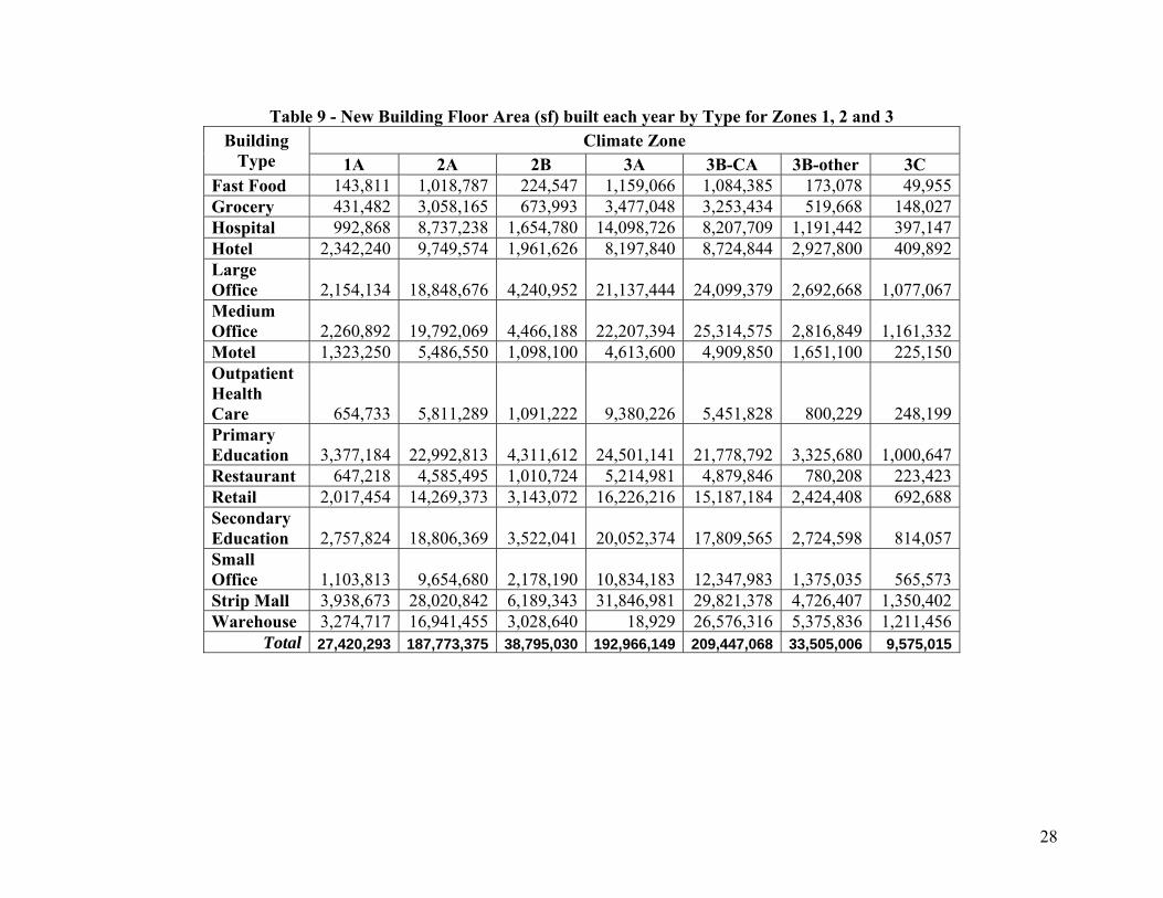
28

Table 9 - New Building Floor Area (sf) built each year by Type for Zones 1, 2 and 3 Climate Zone Building

Type 1A 2A 2B 3A 3B-CA 3B-other 3C Fast Food 143,811 1,018,787 224,547 1,159,066 1,084,385 173,078 49,955Grocery 431,482 3,058,165 673,993 3,477,048 3,253,434 519,668 148,027Hospital 992,868 8,737,238 1,654,780 14,098,726 8,207,709 1,191,442 397,147Hotel 2,342,240 9,749,574 1,961,626 8,197,840 8,724,844 2,927,800 409,892Large Office 2,154,134 18,848,676 4,240,952 21,137,444 24,099,379 2,692,668 1,077,067Medium Office 2,260,892 19,792,069 4,466,188 22,207,394 25,314,575 2,816,849 1,161,332Motel 1,323,250 5,486,550 1,098,100 4,613,600 4,909,850 1,651,100 225,150Outpatient Health Care 654,733 5,811,289 1,091,222 9,380,226 5,451,828 800,229 248,199Primary Education 3,377,184 22,992,813 4,311,612 24,501,141 21,778,792 3,325,680 1,000,647Restaurant 647,218 4,585,495 1,010,724 5,214,981 4,879,846 780,208 223,423Retail 2,017,454 14,269,373 3,143,072 16,226,216 15,187,184 2,424,408 692,688Secondary Education 2,757,824 18,806,369 3,522,041 20,052,374 17,809,565 2,724,598 814,057Small Office 1,103,813 9,654,680 2,178,190 10,834,183 12,347,983 1,375,035 565,573Strip Mall 3,938,673 28,020,842 6,189,343 31,846,981 29,821,378 4,726,407 1,350,402Warehouse 3,274,717 16,941,455 3,028,640 18,929 26,576,316 5,375,836 1,211,456

Total 27,420,293 187,773,375 38,795,030 192,966,149 209,447,068 33,505,006 9,575,015

29

Table 10 - New Building Floor Area (sf) built Each Year by Type for Zone 4 through 8 Climate Zone Building

Type 4A 4B 4C 5A 5B 6A 6B 7 8 Fast Food 2,030,510 64,084 231,611 2,044,135 515,701 574,739 8,578 80,736 5,046Grocery 6,091,133 192,120 696,040 6,132,077 1,546,405 1,725,926 25,196 242,512 0 Hospital 23,961,214 463,338 1,919,545 22,438,817 3,971,472 5,891,017 728,103 529,530 0 Hotel 13,877,772 409,892 1,698,124 14,843,946 4,830,870 3,220,580 731,950 439,170 0 Large Office 47,862,174 1,211,701 5,991,186 42,476,838 9,558,971 12,049,689 1,413,651 1,682,918 0 Medium Office 50,338,818 1,260,169 6,331,733 44,643,347 10,056,644 12,700,529 1,507,261 1,735,821 61,773Motel 7,797,300 229,100 963,800 8,358,200 2,717,600 1,809,100 402,900 240,950 0 Outpatient Health Care 15,983,186 303,830 1,288,069 14,973,271 2,653,166 3,919,839 500,678 372,299 0 Primary Education 53,659,706 1,464,182 5,783,152 62,856,831 9,697,449 10,793,746 1,405,321 2,391,253

220,731

Restaurant 9,137,300 289,032 1,042,642 9,199,362 2,319,346 2,587,099 39,010 363,506 17,732Retail 28,426,184 900,494 3,238,316 28,616,673 7,221,272 8,043,839 121,220 1,134,277 0 Secondary Education 43,909,216 1,196,165 4,734,819 51,435,086 7,941,205 8,838,329 1,146,325 1,960,381

166,134

Small Office 24,557,200 613,930 3,088,573 21,777,695 4,907,235 6,193,965 733,773 845,205 42,050Strip Mall 55,816,616 1,800,536 6,414,410 56,266,750 14,179,221 15,754,690 225,067 2,250,670 0 Warehouse 36,324,751 1,003,237 5,148,688 38,085,148 11,887,412 10,638,098 1,798,255 1,495,391 0

Total 419,773,080 11,401,810 48,570,708 424,148,176 94,003,969 104,741,185 10,787,288 15,764,619 513,466

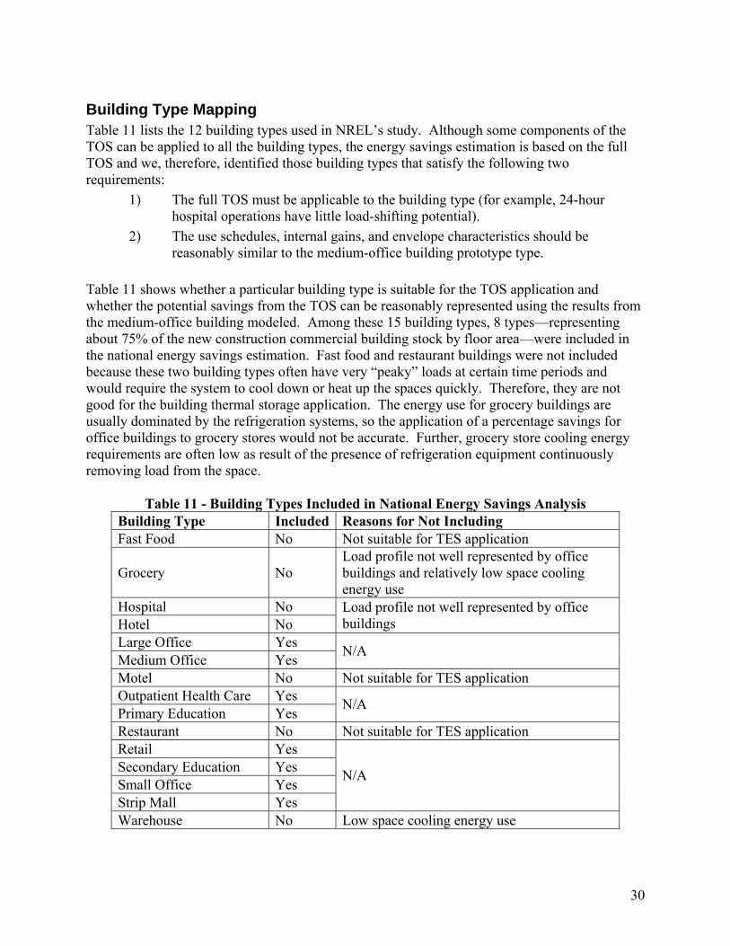
30

Building Type Mapping Table 11 lists the 12 building types used in NREL’s study. Although some components of the TOS can be applied to all the building types, the energy savings estimation is based on the full TOS and we, therefore, identified those building types that satisfy the following two requirements:

1) The full TOS must be applicable to the building type (for example, 24-hour hospital operations have little load-shifting potential).

2) The use schedules, internal gains, and envelope characteristics should be reasonably similar to the medium-office building prototype type.

Table 11 shows whether a particular building type is suitable for the TOS application and whether the potential savings from the TOS can be reasonably represented using the results from the medium-office building modeled. Among these 15 building types, 8 types—representing about 75% of the new construction commercial building stock by floor area—were included in the national energy savings estimation. Fast food and restaurant buildings were not included because these two building types often have very “peaky” loads at certain time periods and would require the system to cool down or heat up the spaces quickly. Therefore, they are not good for the building thermal storage application. The energy use for grocery buildings are usually dominated by the refrigeration systems, so the application of a percentage savings for office buildings to grocery stores would not be accurate. Further, grocery store cooling energy requirements are often low as result of the presence of refrigeration equipment continuously removing load from the space.

Table 11 - Building Types Included in National Energy Savings Analysis

Building Type Included Reasons for Not Including Fast Food No Not suitable for TES application

Grocery No Load profile not well represented by office buildings and relatively low space cooling energy use

Hospital No Hotel No

Load profile not well represented by office buildings

Large Office Yes Medium Office Yes N/A

Motel No Not suitable for TES application Outpatient Health Care Yes Primary Education Yes N/A

Restaurant No Not suitable for TES application Retail Yes Secondary Education Yes Small Office Yes Strip Mall Yes

N/A

Warehouse No Low space cooling energy use

31

The TOS can be applied to portions of hospital and hotel building types; however it is difficult to estimate the potential savings in these two building types from the office building results because their 24/7 operation schedule is very different from the assumed office occupancy schedule. The motel buildings often use packaged terminal air conditioners that must respond quickly to unpredictable occupancy changes, so this building type was also excluded. Warehouse buildings were not included because most warehouses are only semi-heated and the cooling energy use is not significant. In summary, the energy use calculated for the various cases from simulations are applied to 9 climates zones and 8 building prototypes to estimate the national technical energy savings, representing approximately 69% of floor area of total new commercial building stock.

National Energy Savings Estimation The annual national energy savings potential (cooling, fan and pump) from the TOS was estimated by applying the previously described methodology to the energy savings estimated for the medium-office building for each building performance level and for the five selected climate locations, which were described in the case study section. Table 12 summarizes the national energy saving for the full TOS (Case 8), compared to the conventional VAV system with two-speed chiller (Case 1). Note that these annual estimates are for new construction and building-types and climate locations for which the full TOS is applicable (see previous section). Although it is likely that parts of the TOS are applicable for a large portion of the existing commercial building stock and the full TOS may be applicable to a substantial fraction of the existing building stock, we did not estimate that potential in this study, because the primary market – as with most advanced TOS involving systems engineering in building design – is new construction. In this sense, the technical potential we present here is conservative. In addition, the savings estimates are for cooling systems (chiller, fan and pumps) only. If the heating systems savings were to be included, the total savings estimates would also be higher.

Table 12 - Summary of National Technical Site Electricity Savings Potential for the Year 2007 for the Low-Lift Cooling Technology Option Set (assuming 100% Penetration)

National Cooling and Fan and Pump Electricity Savings Building Performance Level

Quad Percentage Baseline Building 0.0098 71%

Mid-Performance Building 0.0048 64%

High Performance Building 0.0028 58% For baseline buildings that are compliant with ASHRAE 90.1-2004, the full TOS saves about 0.0098 quads of site electricity use in one year of new construction with the full TOS being applied to approximately 69% of floor area of total 2007 U.S. new commercial building stock (assuming 100% penetration); the annual site electricity savings are about 0.0048 quads for mid-performance buildings and 0.0028 quads for high-performance buildings. The annual national technical energy savings for different system configurations compared to the conventional VAV system with two-speed chiller (Case 1) are shown in Figure 9. For baseline

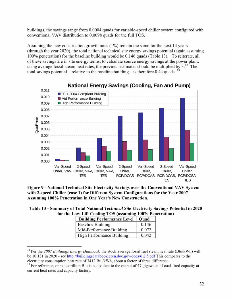
32

buildings, the savings range from 0.0004 quads for variable-speed chiller system configured with conventional VAV distribution to 0.0098 quads for the full TOS. Assuming the new construction growth rates (1%) remain the same for the next 14 years (through the year 2020), the total national technical site energy savings potential (again assuming 100% penetration) for the baseline building would be 0.146 quads (Table 13). To reiterate, all of these savings are in site energy terms; to calculate source energy savings at the power plant, using average fossil-steam heat rates, the previous estimates should be multiplied by 3.12 The total savings potential – relative to the baseline building – is therefore 0.44 quads. 13

National Energy Savings (Cooling, Fan and Pump)

0.000

0.001

0.002

0.003

0.004

0.005

0.006

0.007

0.008

0.009

0.010

0.011

Var-SpeedChiller, VAV

2-SpeedChiller, VAV,

TES

Var-SpeedChiller, VAV,

TES

2-SpeedChiller,

RCP/DOAS

Var-SpeedChiller,

RCP/DOAS

2-SpeedChiller,

RCP/DOAS,TES

Var-SpeedChiller,

RCP/DOSA,TES

Qua

d/Ye

ar

90.1-2004 Compliant BuildingMid Performance BuildingHigh Performance Building

Figure 9 - National Technical Site Electricity Savings over the Conventional VAV System with 2-speed Chiller (case 1) for Different System Configurations for the Year 2007 Assuming 100% Penetration in One Year’s New Construction. Table 13 - Summary of Total National Technical Site Electricity Savings Potential in 2020

for the Low-Lift Cooling TOS (assuming 100% Penetration) Building Performance Level Quad Baseline Building 0.146 Mid-Performance Building 0.072 High Performance Building 0.042

12 Per the 2007 Buildings Energy Databook, the stock average fossil fuel steam heat rate (Btu/kWh) will be 10,181 in 2020 - see http://buildingsdatabook.eren.doe.gov/docs/6.2.5.pdf This compares to the electricity consumption heat rate of 3412 Btu/kWh, about a factor of three difference. 13 For reference, one quadrillion Btu is equivalent to the output of 47 gigawatts of coal-fired capacity at current heat rates and capacity factors.

33

The national technical energy savings in 2020 for different system configurations compared to a conventional VAV system with two-speed chiller are shown in Figure 10. For baseline buildings, the savings range from 0.006 quads for variable-speed chiller system configured with conventional VAV distribution (Case 1) to 0.146 quads for the full TOS (Case 8).

National Energy Savings in 2020 (Cooling, Fan and Pump)

0.00

0.02

0.04

0.06

0.08

0.10

0.12

0.14

0.16

Var-SpeedChiller, VAV

2-SpeedChiller, VAV,

TES

Var-SpeedChiller, VAV,

TES

2-SpeedChiller,

RCP/DOAS

Var-SpeedChiller,

RCP/DOAS

2-SpeedChiller,

RCP/DOAS,TES

Var-SpeedChiller,

RCP/DOSA,TES

Qua

d/Ye

ar

90.1-2004 Compliant BuildingMid Performance BuildingHigh Performance Building

Figure 10 - National Technical Site Electricity Savings in 2020 over the Conventional VAV System with two-speed Chiller (Case 1) for Different System Configurations for 2020 Assuming 100% Penetration over Fourteen Years of New Construction

Acknowledgement Jaclyn Phillips (now at WSU) and Jessica Knappek (U. Eastern Washington-bound) exercised the compressor design tool with great skill and diligence through all one thousand conditions on the analysis grid. We are also profoundly grateful to John Ryan, DOE-BTP, for insightful discussions in the formative stages.

34

References

1. ASHRAE, 2007. ANSI/ASHRAE/USGBC Standard 189P: Standard for High-Performance Green Buildings Except Low-Rise Residential Buildings. Atlanta, GA: American Society of Heating, Refrigerating, and Air-Conditioning Engineers. First Public Review Draft.

2. ANSI/ASHRAE/IESNA. 2004. ASHRAE Standard 90.1-2004, Energy Standard for Buildings Except Low-Rise Residential Buildings, American Society of Heating, Ventilating and Air-Conditioning Engineers, Inc., Atlanta, Georgia.

3. Braun, J.E., J.W. Mitchell, S.A. Klein. 1987a. Models for variable-speed centrifugal chillers, ASHRAE Trans. 93(1):1794-1813.

4. Braun, J.E., J.W. Mitchell, S.A. Klein, 1987b. Performance and control characteristics of a large cooling system, ASHRAE Trans. 93(1):1830-1852.

5. Braun, J.E., S.A. Klein, W.A Beckman, J.W. Mitchell. 1989a, Methodologies for optimal control of chilled water systems without storage, ASHRAE Trans. 95(1):652-662.

6. Braun, J.E., S.A. Klein, J.W. Mitchell, W.A. Beckman. 1989b, Applications of optimal control to chilled water systems without storage, ASHRAE Trans. 95(1):663-675.

7. Braun, J.E., S.A Klein and J.W Mitchell. 1989c. Effectiveness models for cooling towers and cooling coils. ASHRAE Trans. 95(2):164-174.

8. Braun, J.E., G.T. Diderrich. 1990. Near-optimal control of cooling towers for chilled water systems, ASHRAE Trans. 96(2):806-813.

9. Briggs, R.S., R.G. Lucas, and Z.T. Taylor. 2002. Climate Classification for Building Energy Codes and Standards. Pacific Northwest National Laboratory, Richland, WA. <http://www.energycodes.gov/implement/climatezones_04_faq.stm>

10. Energy Information Administration (EIA). 2003. 2003 Commercial Building Energy Consumption and Expenditures (CBECS), Public Use Data, Micro-data files: http://www.eia.doe.gov/emeu/cbecs/cbecs2003/public_use_2003/cbecs_pudata2003.html.

11. Huang, J., and E. Franconi. 1999. Commercial Heating and Cooling Loads Component Analysis, LBL-37208, Lawrence Berkeley National Laboratory, California.

12. Jarnagin, R.E., B. Liu, D.W. Winiarski, M.F. McBride, L. Suharli, and D. Walden. 2006. Technical Support Document: Development of the Advanced Energy Design Guide for Small Office Buildings, PNNL-16250, Pacific Northwest National Laboratory, Richland, WA.

35

13. Long, N., B. Griffith and P. Torcellini, 2007. Evaluation of the ASHRAE Standard 189P. National Renewable Energy Laboratory, Internal Report Draft, August 2007.

14. 2007 Buildings Energy Databook, http://buildingsdatabook.eren.doe.gov/docs/6.2.5.pdf

15. CUAC, 2004. Technical Support Document: Energy Efficiency Program For Commercial And Industrial Equipment: Commercial Unitary Air Conditioners And Heat Pumps. U.S. Department of Energy, Assistant Secretary, Office of Energy Efficiency and Renewable Energy, Building Technologies Program, Appliances and Commercial Equipment Standards.

36

Appendix A. Literature Review

37

Appendix A. Literature Review January 2007 Letter Report to DOE Building Technology Program Literature Review of Low-Lift, DOAS, Peak-shifting and Related Technologies and Practices This literature review was conducted in support of PNNL's Low-Lift Cooling work for Department of Energy/Building Technology Program (DOE/BTP) and constitutes the first deliverable specific in the Statement of Work. The previous work found to be relevant to the low-lift cooling project’s technical approach may be summarized as follows. Night pre-cooling has been demonstrated in a few large buildings in which high cooling and distribution efficiencies under low-ambient part-load conditions are exhibited. Results of night pre-cooling have been less successful in small buildings, where constant volume night fan operation is a significant penalty (relative to large buildings, where fan speed and static pressure can typically be adjusted by the control system) and existing packaged equipment efficiency does not improve much as ambient temperature drops. The performance gap between small and large cooling equipment, together with the continually falling costs of microprocessor-based packaged-unit controls and high efficiency variable speed motors and drives present a strong motivation to develop low-lift package cooling equipment technologies for mild climates and climates with cool nights. With active core cooling and dedicated outdoor air-conditioning (A/C) systems (DOAS), the energy benefits can be extended to hot and humid climates. Refrigerant-side free-cooling has been mentioned but details of design and performance were not found in the literature, probably because this design traditionally has had little attraction when used with 1) the low chilled-water temperatures required for conventional air-handling unit (AHU) and fan-coil latent-plus-sensible cooling distribution systems, 2) systems that used discrete cool storage, or 3) systems with cooling towers. The energy and market potentials for the refrigerant-side economizer option in buildings with radiant cooling and small air-cooled chiller plants should be explored. The DOE Commercial Unitary Air Conditioner report (2004) found that the best path for getting package equipment from EER-10 to EER-12 was to increase evaporator and condenser size. The question of how to best improve annual performance, particularly with radiant panel (or radiant slab) chilled water temperatures and for the distributions of outdoor conditions experienced with peak shifting controls will have to be addressed further. There appear to be no studies of national energy potential even for buildings with chillers that would provide good low-lift performance. Recent work by proponents of radiant cooling has focused on accurately estimating panel capacity, on modeling the interactions of convection and radiation, and on supervisory control strategies of decoupled dehumidification/ventilation and sensible cooling systems that ensure comfort and acceptable indoor-air quality (IAQ) while avoiding condensation under all conditions. One paper estimates fan energy and higher-air-temperature-effected savings. The loss of air-side free cooling potential has been noted but the potential national impact has not been isolated. The effectiveness and national potential of water- and refrigerant-side economizers in conjunction with radiant cooling, where savings should be greater than for non-DOAS systems, have not been evaluated. The potential system efficiency improvements of active core cooling combined with peak-shifting and efficient low-lift chiller equipment have not been carefully assessed.

38

Work on active core cooling has addressed thermal occupancy conditions such as strong vertical temperature gradients. The considerable challenge of control during diurnal and shorter load transients seems to need more work. The potential system efficiency improvements of slab cooling combined with peak-shifting and efficient low-lift chiller equipment have not been assessed. Work on DOAS has focused on proper control over the wide range of outdoor conditions that such systems face, and on performance-cost-pressure drop considerations—trade-offs to which package A/C plants are particularly sensitive. It is interesting that there are few design integration problems because DOAS provide a predominantly stand-alone function. Supervisory control of reheat is one area of interaction with the radiant cooling that may need further study. Static chiller optimization has been applied to large plants both with and without discrete cool storage. The technical potential of radiant cooling with small package chillers optimized for low-lift conditions has not been addressed. Organization of the Literature Review. The review is organized by topic as follows:

High Performance Buildings and Associated Technologies Discrete Cool Storage Cooling Load Peak Shifting Controls Zone Thermal Response Models and Model Order Reduction Inverse Models Load Forecast-Based Control Vapor-Compression Cycle Efficiencies and Advanced Package A/C Compressor and Equipment Ratings and Performance Maps Enthalpy recovery and Dedicated Outdoor Air Systems (DOAS) Cooling by Radiant Panels Radiant Cooling Integration with DOAS Radiant Cooling and Chiller or Heat Pump Coefficient of Performance (COP) Active Core Cooling Low Fan Power and Displacement Ventilation Static Chiller Optimization Technical Potential and Market Assessments

There do not appear to be any economic analyses of small package low-lift equipment or small package DOAS conditioning equipment for the logical reason that such equipment is not currently produced in any standard product line. One paper was found that provided a credible comparison of radiant cooling to conventional variable air volume (VAV) systems—see the section on Cooling by Radiant Panels. The questions of equipment, mechanical space, and construction costs will have to be revisited when the project moves to the next stage-gate phase. Reference building descriptions are being compiled by the Commercial Benchmark Review task and will be used to guide the final estimates of national energy potential under the Low-Lift Cooling task. Each topical review is followed by a topical bibliography which, in a few cases, may include pertinent reference material not cited in the narrative.

39

High Performance Buildings (HPB) and Associated Technologies High performance can be achieved at relatively low risk by combining off-the-shelf high-performance equipment, good design, commissioning, and ongoing attention to control, operation and maintenance. These practices are described and documented with sufficient completeness for most purposes in the references mentioned below. Standard 90.1 (ANSI 1999, 2004) can serve as a good basic energy performance baseline for this and related HPB and NZEB (net zero energy buildings) research and development, commercial-ization, and market transformation projects. How far one can cost-effectively extend building performance beyond such standards depends on many owner/architectural considerations as well as occupancy- and climate-specific factors. Conventional wisdom holds that performance can be improved up to 30% cost-effectively and that margins up to 50% can be reasonably contemplated.

Hydeman (2003) provides best practice VAV design guidance to achieve energy savings up to 12% compared to “standard practice” with no additional construction cost. Prescriptive extensions (“one possible way”) to achieve energy savings of up to 30% beyond ASHRAE 90.1-1999 are described in the ASHRAE Advanced Energy Guides (ASHRAE 2004, 2006). These extensions address performance levels and integration of the following building subsystems: • Envelope (roof wall floor window door elements) • Lighting (daylighting, interior lighting, task lighting, controls) • Mechanical equipment (heating/cooling equipment efficiencies, supply fans, ventilation, ducts) • Service water heating (equipment efficiencies, pipe insulation)

The “HVAC3” report (TIAX 2002) examines 55 technology options for heating, ventilation and air conditioning (HVAC) and recommends 15 for development/commercialization/market push. These options have been selected with the expectation that they could become cost-effective alone or in combination with other integrated energy design features: • Advanced control, • Dedicated outdoor air-conditioning systems (DOAS), • Displacement ventilation (DV) and under-floor air distribution (UFAD), • Electrically commutated motors (ECM), in either constant- or variable-speed-drive (VSD), • Energy recovery ventilation (ERV), • Cold-climate heat pumps (HP), • Duct-sealing, • Liquid desiccant air conditioning (A/C), • Micro-channel heat exchangers (HX), • Task-ambient A/C, • Phase-change material thermal energy storage (PCM-TES), • Ceiling panel (or chilled beam) cooling, • Small centrifugal compressors, • Fault detection and diagnosis (FDD), • Variable volume refrigeration (VRV) also known as the multi-evaporator split system.

Directions for ongoing research, design guides and commercialization efforts are documented in the roadmap documents of the DOE (BTS 2000a, 2000b, 2001) and the Air-Conditioning and Refrigeration Technology Institute (ARTI 2004).

40

1. ANSI, 1999. ANSI/ASHRAE/IESNA Standard 90.1-1999: Energy Standard for Buildings

Except Low-Rise Residential Buildings. ASHRAE, Atlanta, GA 2. ANSI, 2004. ANSI/ASHRAE/IESNA Standard 90.1-2004: Energy Standard for Buildings

Except Low-Rise Residential Buildings. ASHRAE, Atlanta, GA 3. ASHRAE, 2004, Advanced Energy Design Guide For Small Office Buildings, ASHRAE

(AIA, IES, NBI, DOE) Publication: Atlanta, Georgia. 4. ASHRAE, 2006, Advanced Energy Design Guide For Small Retail Buildings, ASHRAE

(AIA, IES, GBC, DOE) Publication: Atlanta, Georgia. 5. ARTI, 2004. Research Roadmap, Air-conditioning and Refrigeration Technology Institute,

http://www.arti-21cr.org/documents/roadmap.pdf 6. BTS, 2000a, High Performance Commercial Buildings: A Technology Roadmap, U.S. DOE

http://www.eere.energy.gov/buildings/info/documents/pdfs/roadmap_lowres.pdf 7. BTS, 2000b. Lighting Technology Roadmap, U.S. DOE, Washington, D.C.

http://www.eere.energy.gov/buildings/info/documents/pdfs/lighting_roadmap_compressed.pdf

8. BTS, 2001. Building Envelope Technology Roadmap, U.S. DOE, Washington, D.C. http://www.eere.energy.gov/buildings/info/documents/pdfs/envelope_roadmap.pdf

9. Hydeman, M., et al, 2003. Advanced VAV System Design Guide, CEC 500-03-082-A11, California.

10. Steven Winter Associates, Inc., 2004, GSA/LEED® Cost Study. 11. TIAX, 2002. Energy Consumption Characteristics of Commercial Building HVAC Systems,

Volume III: Energy Savings Potential, DOE-BT, Cambridge, Massachusetts. http://www.tiax.biz/aboutus/pdfs/HVAC3-FinalReport.pdf

12. U.S. General Services Administration, 2003. Facilities Standards, www.gsa.gov/Portal/gsa/ep

13. U.S. General Services Administration, 2004. Design and Construction Delivery Process, www.gsa.gov/Portal/gsa/ep/contentView.do?contentType=GSA_BASIC&content id=10366.

14. http://www.wbdg.org/references/ccbdoc.php?i=280.

Discrete Cool Storage The literature on discrete cool storage is extensive. One of the earliest well-monitored demonstrations of discrete cool storage made use of a solar heated rock bed, which would otherwise have sat idle in summer, to reject heat to the night air (Karaki 1978). In the hey-day of utility demand-side management programs, many large-scale water and ice-storage systems were deployed. Calobrisi et al. (1980) develops control strategies for dual (hot and cold) storage as well as chilled water storage systems. The push to make discrete cool storage save energy as well as demand-charge dollars has put added pressure on chiller manufacturers to improve part-load and off-design condition efficiencies. Methodical and rational strategies for controlling charging operations and for sharing the load between chiller and storage discharge operations were developed by Braun and Henze (see next section on Cooling Load Peak-shifting Controls).

41

Recent work has re-introduced phase change materials (PCM) which have a long history in heating (Telkes and Raymond 1949, wallboard applications in the 1980’s), for discrete cool storage. Buddhi (2000) provides an extensive PCM bibliography with 590 citations. Note that PCMs may be used for both heating and cooling and for both intrinsic and discrete thermal storage, depending on the phase change temperature range, encapsulation technique, thermal delivery mechanism, and so on. According to TIAX (2002 – previously listed) PCM TES realizes energy savings on the order of 10% for water-cooled systems, a value that corresponds closely with the chilled water storage savings for retrofit applications cited in CEC (1996). Moreover, air-cooled systems with TES are said to achieve ~20% energy savings relative to conventional air-cooled designs. In the analyses executed and reviewed by TIAX, ice-based cooling generally consumed more energy due to lower COP of the vapor compression cycle at low evaporator temperatures. 1. Buddhi, D. 2000. Selected references (1900 - 1999) on phase change materials and latent

heat energy storage systems, http://www.fskab.com/annex17/Bibliography.pdf. 2. Calobrisi, G., et al. 1980. Comparison of performance and computer simulation of a thermal

storage system for commercial buildings, ASHRAE Trans. 86(1):336-350. 3. California Energy Commission. 1996. Source Energy And Environmental Impacts of

Thermal Energy Storage. http://www.energy.ca.gov/reports/500-95-005_TES-report.pdf. 4. Karaki, S. 1978. Air conditioning by nocturnal evaporative cooling of a pebble-bed, DOE

Solar Cooling Conference, 15-17 Feb 1978, San Francisco, California. 5. Telkes, M. and E. Raymond. 1949. Storing solar heat in chemicals, Heating and Ventilating,

(1949): 80-86

Cooling load peak shifting controls Activities in the passive-solar research community, 1975-80, as well as three pioneering papers (Stoecker et. al. 1981), Perkins 1984, Eto 1984) suggested to the HVAC community the potential of using building thermal mass to shift peak cooling loads. Stoecker et al. used a masonry test building to validate a transfer function model that was then used to simulate peak-shifting controls with room temperature swings of up to 12°F. From 1990 on, most work has involved variations and improvements on a single basic approach: predict driving functions out to a control horizon (up to 7 days (Henze 1997) but usually only 1 day) and adjust hourly setpoints such that total building electricity cost, based on simulated thermal response, is minimized. A number of variations have focused on practicality and robustness of implementation. Braun developed simple control rules by examination of the behaviors of simulated systems under optimal control. Brandemuehl, Morris and Braun (2002a) used instrumented test cells to demonstrate precooling performance. Braun (2002b) describes a thermal network-based model to be embedded in the controller. Recent work of Braun (2005) has focused on demand and RTP-rate responsive peak shifting controls. Sun (2006) surveys dozens of electric utility rate structures—existing and proposed—and develops a generic RTP rate model based on season, time of day, daytype and outdoor temperature. A set of prototypical building descriptions is compiled and used to validate the load-profile tool, Site-Pro, against DOE-2. Existing TES design and control configurations that have been found useful under many kinds of TOU rate are described. Braun (2006) develops baseline optimal control sequences and assesses several simpler suboptimal control sequences by

42

comparing annual simulation results. He treats economizer as stage-1 cooling, then assigns a 69°F setpoint for stage-1 cooling and a 75°F setpoint for stage-2 mechanical cooling. The best near-optimal control strategy results in annual operating costs only a few percent higher than true optimal control; annual energy results are not compared. Armstrong et al. (2006) describes a CRTF-based model (see Zone Thermal Response section) and several algorithms for obtaining near-optimal control of night pre-cooling and annual energy as well as annual cost results. 1. Andresen I. and M J. Brandemuehl, 1992. Heat storage in building thermal mass - a

parametric study. ASHRAE Trans. 98(1):910-18 2. Armstrong, P.R., S.B. Leeb and L.K. Norford. 2006b. Control with building mass – Part II:

simulation. ASHRAE Trans. 112(1). 3. Brandemuehl, M.J., M.J. Lepoer and J.F. Kreider, 1990. Modeling and testing the interaction

of conditioned air with building thermal mass, ASHRAE Trans. 96(2):871-75. 4. Braun, J.E., 2006. Interaction Between Dynamic Electric Rates and Thermal Energy Storage

Control - Phase II, ASHRAE 1252-RP, Final Report. 5. Braun, J E., 1990. Reducing energy costs and peak electrical demand through optimal control

of building thermal storage, ASHRAE Trans. 96(2):876-88. 6. Braun, J.E., K.W. Montgomery and N. Chaturvedi. 2001. Evaluating the performance of

building thermal mass control strategies. Int’l J. HVAC&R Research 7(4):403-28. 7. Braun, et al, J.E., T.M. Lawrence,, C.J. Klaassen and J.M. House. 2002a. Demonstration of

load shifting and peak load reduction with control of building thermal mass. Proceedings of the 2002 ACEEE Summer Study on Energy Efficiency in Buildings.

8. Braun, J.E. and N. Chaturvedi, 2002b. An inverse grey-box model for transient building load prediction. Int’l J. HVAC&R Research 8(1):73-99.

9. Braun, J.E., 2003. Load control using building thermal mass, ASME JSEE 125:292-301 10. Braun, J.E. and K. Mercer, 2003. VSAT: Ventilation Strategy Assessment Tool, CEC-500-

2005-011, http://www.energy.ca.gov/2005publications 11. Braun, J.E. and Z. Zhong,2005. Development and evaluation of a night ventilation precooling

algorithm, Int'l J. HVAC&R Research, 11(3). see also http://www.archenergy.com/cec-eeb/P3-LoadControls

12. Conniff, J.P., 1991. Strategies for reducing peak air conditioning loads by using heat storage in the building structure, NY-91-10-2, ASHRAE Trans. 97(1) 704-709.

13. Eto, J.H., 1984. Cooling strategies based on indicators of thermal storage in commercial building mass, Annual Symposium on Improving Building Energy Efficiency in Hot and Humid Climates, ESL, Texas A&M University, College Station, Texas.

14. Henze, G.P., R.H. Dodier and M. Krarti. 1997. Development of a predictive optimal controller for thermal energy storage systems. Int’l J. HVAC&R Research, 3(3):233-64.

15. Keeney, K. and J. Braun. 1996. A simplified method for determining optimal cooling control strategies for thermal storage in building mass, Int’l J. HVAC&R Research 2(1):59-78.

16. Keeney, K R., and J.E. Braun. 1997. Application of building pre-cooling to reduce peak cooling requirements. ASHRAE Trans. 103(1):463-69.

43

17. Morris, F B., J.E. Braun and S.J. Treado. 1994. Experimental and simulated performance of optimal control of building thermal performance. ASHRAE Trans. 100(1):402-14.

18. Perkins, D. 1984. Heat balance studies for optimising passive cooling with ventilation air, ASHRAE Journal, 26(2):27-29.

19. Rabl, A. and L.K. Norford, 1988. Peak load reduction by preconditioning buildings at night. 5th Annual Symposium on Improving Building Efficiency in Hot and Humid Climates.

20. Rabl, A. and L.K. Norford, 1991. Peak load reduction by preconditioning buildings at night. Int’l J Energy Res. 15:781-98.

21. Ruud, M.D., J.W. Mitchell and S.A. Klein. 1990. Use of building thermal mass to offset cooling loads, ASHRAE Trans. 96(2):820-29.

22. Stoecker, W.F., R.R. Crawford, S. Ikeda, W.H. Dolan, and D.J. Leverenz, 1981. Reducing the peak of internal air-conditioning loads by use of thermal swings. ASHRAE Trans. 87(2):599-608.

23. Sun, C, T. Rossi and K. Temple, 2006. Interaction Between Dynamic Electric Rates and Thermal Energy Storage Control - Phase I, ASHRAE 1252-RP, Final Report.

Zone Thermal Response Models and Model Order Reduction Peak shifting cannot be effectively accomplished without use of advanced controls that predict the thermal response of the building envelope, structure, partitions and zone contents. The dynamics are governed by the distribution of mass, conduction and other heat transfer elements, which together form a thermal network or a collection of interconnected sub-networks. The conduction transfer function (CTF) method of calculating transient thermal response of multi-layer walls was developed from early work by E. Smith and L. Pipes (1941) for routine application in peak cooling load calculations by Mitalas (1965, 1968 and 1972), Stephenson and Mitalas (1971) Davies (1973). Green (1979) and Ceylan (1980) showed that more elaborate thermal networks, e.g. combinations of walls, could be combined into a single transfer function. Balcomb (1983) proposed an interesting method of model order reduction applied to network models. Walton’s (1983) incorporation of CTF submodels into the TARP program is one of the first rigorous, well documented, widely-used implementations. Seem (1987) shows that CTF models can be combined analytically to form a whole-zone transfer function. Strand (1997) describes a heat source transfer function model (HSTF) for BLAST to simulate the response delays of any specified radiant slab heating or cooling subsystem. Spitler (1997 and 1999) developed an ingenious method of peak load (actually periodic load) calculation using CTFs that can be implemented in a spreadsheet. 1. Balcomb, J.D. 1983. Thermal network reduction. Proc. Annual ASES Conf., Minneapolis,

MN. LA-UR-83-869, LA-9694-MS 2. Ceylan, H.T, and G.E. Myers. 1980. Long-time solutions to heat conduction transients with

time-dependent inputs. ASME J. Heat Transfer 102(1):115-20. 3. Davies, M.G. 1973. The thermal admittance of layered walls. Building Science 8:207-20 4. Green, M.D. and A. Ulge. 1979. Frequency- and time-domain thermal response of

dwellings. Building and Environment 14:107-18.

44

5. Horn, J.C., 1982. Investigation of various thermal capacitance models; M.S. Thesis, M.E. Dept, University of Wisconsin, Madison, WI.

6. Mitalas, G.P. 1965. An assessment of common assumptions in estimating cooling loads and space temperatures. ASHRAE Trans. 71 (II).

7. Mitalas, G.P. 1968. Calculation of transient heat flow through walls and roofs. ASHRAE Trans. 74: 182-188.

8. Mitalas, G.P. 1972. Transfer function method of calculating cooling loads, heat extraction rate, and space temperature. ASHRAE Journal 14(12): 52.

9. Pipes, L.A. 1957. Matrix analysis of heat transfer problems. Franklin Institute Journal 263(3). 10. Seem, J.E. 1987. Modeling of Heat Transfer in Buildings. PhD thesis, Univ. Wisconsin. 11. Smith, E.G. 1941a. A simple and rigorous method for the determination of the heat

requirements of simple intermittently heated exterior walls, Journal of Applied Physics 12 (August).

12. Smith, E.G. 1941b. The heat requirements of simple intermittently heated interior walls and furniture, Journal of Applied Physics 12 (August).

13. Smith, E.G. 1942. A method of compiling tables for intermittent heating, Heating, Piping and Air Conditioning 14(6).

14. model into an integrated building energy analysis program, ASHRAE Trans. 103(1):949-958. 15. Spitler, J.D.and D.E. Fisher, 1999. On the relationship between the radiant time series and

transfer function methods for design cooling load calculations, IJHVAC&R Research 5(2). 16. Stephenson, D.G., and G.P. Mitalas. 1971. Calculation of heat conduction transfer functions

for multi-layer slabs. ASHRAE Trans. 77(2). 17. Strand, R.K. and C.O. Pedersen. 1997. Implementation of a radiant heating and cooling 18. Walton, G. N. 1983. Thermal Analysis Research Program (TARP). NBSIR 83-2655.

Inverse Models To implement controls that can anticipate and shift the cooling load it is necessary to obtain a response model that represents the building as built and occupied. Pawelski (1979) and Seem (1985) used least-squares to obtain transfer function models from an engineering description. Seem (1987) introduced the term comprehensive room transfer function (CRTF) to describe a multi-input transfer function representation of zone temperature response to zone heat rate and exogenous drivers such as sol-air temperatures on one or more exterior walls and he also developed practical and elegant methods of computing a reduced order CRTF from the zone’s engineering description. Subbarao (1985), Barakat (1987) and Taylor (1988) present various methods to overcome some of the problems, such as instability, with models obtained from direct application of least-squares regression to time series of measured conditions and responses. Armstrong (2000, 2006) formulated a constrained search for CRTF model coefficients based on a CTF property demonstrated by Hittle (1983) and applied the method to training and testing time-series data sets ranging from several days to several months duration. 1. Armstrong, P.R., et al, 2000. Russian apartment building thermal response models for

retrofit selection and verification, ACEEE Summer Study on Energy Efficiency in Buildings.

45

2. Armstrong, P.R., S.B. Leeb and L.K. Norford. 2006. Control with building mass – Part I: thermal model. ASHRAE Trans. 112(1).

3. Barakat, S.A., 1987. Experimental determination of the z-transfer function coefficients for houses, ASHRAE Trans., 93 (1) 3022.

4. Hittle, D.C. and R. Bishop. 1983. An improved root-finding procedure for use in calculating transient heat flow through multilayered slabs. Int’l J Heat Mass Transfer 26(11):1685-93.

5. Pawelski, M.J., J.W. Mitchell and W. A. Beckman. 1979. Transfer functions for combined walls and pitched roofs. ASHRAE Trans. 85(2).

6. Seem, J.E. and C.E. Hancock. 1985. A method for characterizing the performance of a thermal storage wall from measured data, Thermal Performance of the Exterior Envelopes of Buildings III, ASHRAE SP-49:351-363, ASHRAE/DOE/BTECC, Clearwater Beach, FL.

7. Seem, J.E. 1987. Modeling of Heat Transfer in Buildings. PhD thesis, Univ. Wisconsin. 8. Seem, J.E., S.A. Klein, W.A. Beckman and J.W. Mitchell, 1987. Transfer functions for

efficient calculation of multi-dimensional transient heat transfer, HTD; V.78, pp. 25-33, ASME J. Heat Transfer, New York.

9. Seem, J.E., S.A. Klein, W.A. Beckman and J.W. Mitchell, 1989a .Comprehensive Room Transfer Functions for Efficient Calculation of the Transient Heat Transfer in Buildings, ASME J. Heat Transfer V.111,No.2, pp.264-273, (1989a) New York.

10. Seem, J.E., S.A. Klein, W.A. Beckman and J.W. Mitchell. 1989b. Model reduction of transfer functions by the dominant root method. ASME J. Heat Transfer, New York.

11. Subbarao K., Burch J., Hancock E., Jeon H., 1985. Measurement of effective thermal capacitance in buildings, Thermal Performance of the Exterior Envelopes of Buildings III, ASHRAE/DOE/BTECC, Clearwater Beach, FL.

12. Subbarao, K. 1985. Thermal Parameters for Single and Multizone Buildings and their Deter-mination from Performance Data, Solar Energy Research Institute Report SERI/TR-253-2617.

13. Taylor, Z.T and R.G. Pratt. 1988. The effect of model simplifications on equivalent thermal parameters calculated from hourly building performance data; Proc. ACEEE, 10:268-78.

Load Forecast-Based Controls In addition to an accurate thermal response model, night precooling controls require forecasts of weather and internal gains (i.e. light and plug loads). In recent years it has become possible to routinely and reliably download weather forecasts (by FTP or XML) from the national weather service. Internal gains, on the other hand are building specific. Forrester (1984) and Seem (1991) have developed adaptive forecast algorithms; Seem uses 1- or 7-day differencing (look-back regression) to provide reliable internal gain forecasts from past measured time-series of light, plug or whole-building loads. Kintner-Meyer (1995) and Henze (1997) have modeled and simulated typical buildings with charging and discharging of cold storage controlled to take advantage of time-of-use rates. Henze (1999) assessed the impact of realistic forecast uncertainties on annual operating costs of peak-shifting controls and found the impact to be relatively small in terms of annual operating cost. The role of load forecasting in demand response is discussed very briefly in TIAX (2002 previously referenced) and more thoroughly in

46

the forthcoming ASHRAE HVAC Applications Handbook chapter on Supervisory Control Strategies and Optimization (2007). 1. ASHRAE, 2007. ASHRAE HVAC Applications Handbook, in press; Chapter 41 manuscript

approved by TC 7.4 July 18, 2006. 2. Forrester, J.R. and W.J. Wepfer. 1984. Formulation of a load prediction algorithm for a

large commercial building. ASHRAE Trans. 90(2B). 3. Henze, G.P., R.H. Dodier and M. Krarti. 1997. Development of a predictive optimal

controller for thermal energy storage systems. Int’l J. HVAC&R Research, 3(3):233-64. 4. Henze, G.P. and M. Krarti. 1999. The impact of forecasting uncertainty on performance of a

predictive optimal controller for thermal energy storage systems. ASHRAE Trans. 105(1):553.

5. Kintner-Meyer, M. and A.F. Emery. 1995. Cost optimal analysis and load shifting potentials of cold storage equipment, ASHRAE Trans. 101(2):539-48.

6. Seem, J.E. and J.E. Braun. 1991. Adaptive methods for real-time forecasting of building electrical demand. ASHRAE Trans. 97(1):710-21.

Vapor-Compression Cycle Efficiencies and Advanced Package A/C Cooling efficiency improvements have generally been approached quite differently depending on the size of plant involved. Use of variable-speed compressors is one of the most effective paths to good part-load efficiency but it is typically used only in large (>50 Ton) chillers (Kallen 1982). Although most compressors operate more efficiently at lower speeds, centrifugal, scroll and screw compressor start to lose efficiency below about 50% rated speed (Brasz 2006) whereas reciprocating and rolling piston compressor efficiencies continue to rise down to 25% or less of rated speed14. Small package equipment manufacturers have relied on incremental improvements in motor, fan and compressor efficiencies, incrementally larger (or more effective) condensers and evaporators, less restrictive air flow paths, improved refrigerant flow control, improved compressor and condenser fan sequencing, and better leak-tightness and thermal insulation of the cabinet (ADL 2000, Chiu 1987, CUAC 2004). Products that convert air-cooled equipment to use some amount of evaporative cooling (Armstrong 2006; micro spray) have been introduced but are widely perceived as extra maintenance burden. Efficiency gains in larger systems have mainly been achieved by variable-speed compressors, more efficient compressors, improved inter-stage cooling, and variable-speed pumps and condenser fans (Chiu 1987). Considerable work has gone into redesigning A/C equipment for chlorofluorocarbons (CFC) replacements (Kruse 1992, ARI 2003). Uncertainty in achievable performance (capacity and EER) and costs of redesign are major barriers to adoption of any new refrigerant. An additional barrier to using hydrocarbons or ammonia is safety (ICARMA 2003 cites EPA prohibition on A3 refrigerants in occupied buildings). Also ammonia is incompatible with the copper tubing used 14 Constant-speed cylinder unloading--theoretically applicable to multi-rotor vane and rolling-piston compressors as well as to multi-cylinder reciprocating compressors--is more efficient than hot gas bypass but still results in efficiency decreasing with decreasing capacity as shown by Garland, 1980. The conventional wisdom that all A/C equipment starts to lose efficiency at some fraction of nominal capacity no doubt stems from such duty-cycle and unloading characteristics which, in turn, are a legacy from when virtually all compressors were operated at constant speed.

47

in virtually all package equipment currently produced for building A/C and heat pump applications. Barriers to use of zeotropic refrigerants are loss of correct charge proportions, need for service people to carry additional tanks, and difficulty to restore charge to correct proportions. As industry moves toward improved fault detection and diagnostic systems that incorporate sensors for refrigerant suction temperature and pressure (or evaporating or condensing temperature and pressure) early leak detection could mitigate the problem of maintaining correct charge proportions. Rice (1990) addresses the practical issues, as well as documenting measured efficiency gains by compressor downsizing in residential equipment. Holtzapple (1989) has assessed methods of improved desuperheating that result in improved performance without increased condenser size. However, throughout most of these efforts, the conditions targeted for efficiency improvements (ICARMA 2003, CUAC 2004) have been ARI full- or part-load rating conditions (ARI 340 & 550) for cooling equipment. Continuing on this path will make it very difficult to reach NZEB. Integrated design represents an alternate path that should eventually move the industry significantly closer to net ZEB. Peak-shifting changes the load shape by moving loads to times of lower outdoor ambient temperature. Radiant and chilled-beam cooling result in higher evaporator temperatures. These effects, together with increased evaporator and condenser surface areas, present a chiller with much lower pressure ratios than those seen in today’s HVAC applications, e.g. 1.5:1 (85/55F) instead of 3:1 (120/50F). One researcher in Japan (where energy costs make buyers more attentive to SEER than EER) has looked at efficient low-lift compressor design. Takebayashi (1994) reports design and testing of a residential-size variable-speed, variable-compression-ratio scroll compressor claimed to be more efficient under all load and pressure-ratio conditions than a standard rolling-piston compressor. A few of the proponents of hydronic radiant cooling also mention potential primary cooling efficiency gains. In general, however, research investment in small low-lift cooling equipment has been absent. 1. ADL, 2000, Energy Efficient Rooftop Air Conditioner: Continuation Application Technical

Progress Statement, Presentation on 7 November, Project #: DE-FC26-99FT40640. 2. Chiu, S.A., F.R. Zaloudek, 1987. R&D Opportunities for Commercial HVAC Equipment,

PNL-6079 3. CUAC, 2004. Technical Support Document: Energy Efficiency Program For Commercial

And Industrial Equipment: Commercial Unitary Air Conditioners And Heat Pumps. U.S. Department of Energy, Assistant Secretary, Office of Energy Efficiency and Renewable Energy, Building Technologies Program, Appliances and Commercial Equipment Standards.

4. Garland, M.W., 1980. Compressor capacity control for air-conditioning system partial load operation, , ASHRAE Trans. 88(1):477-484.

5. Goetzler, W., and J. Dieckmann, 2001. Assessment of the Commercial Implications of ASHRAE A3 Flammable Refrigerants in Air-Conditioning and Refrigeration Systems, ARTI 21CR/610-50025-01

6. Holtzapple, M.A., 1989. Reducing energy costs in vapor-compression refrigeration and air conditioning using liquid recycle—Parts I-III, Paper Nos. 3221-3223, ASHRAE Trans. 95(1).

48

7. IEA, 1996. Annex 28 - Low Energy Cooling, Subtask 2: Reference Building Description. International Energy Agency, Zürich, Switzerland.

8. IIR/Kruse, 1992. Compression Cycles for Environmentally Acceptable Refrigeration, Air Conditioning and Heat Pump Systems, pp.10-13 history, technology taxonomy, application taxonomy) Int'l Inst. of Refrigeration, Paris.

9. Kallen H.P., 1982. Analysis - off peak cooling methods to reduce energy consumption, ASHRAE Journal, 24(12) 30-33.

10. Brasz, J.J., 2006. Comparison of part-load efficiency characteristics of screw and centrifugal compressors, International Compressor Conference at Purdue.

11. Marques, M.E., P.A. Domanski. 1998. Potential coefficient of performance improvements due to glide matching with R-470C. International Refrigeration Conference at Purdue.

12. ICARMA, 2003. Survey of Available Literature on the Use of Hydrocarbon Refrigerants for HVAC&R Applications. Int’l Council of A/C and Refrigeration Manufacturers' Associations

13. Stoecker, W.F., H. Kruse, D. Didion, 1986. Recent Advances in Refrigeration Machinery: Design, Manufacture and Application, U.S. Nat'l Committee of the IIR Short Course, Purdue.

14. Stoecker, W. 1989. Growing opportunities for ammonia refrigeration, Proc. Int'l Inst. Ammonia Refrigeration; reprinted in CFC's Time of Transition, pp.128-139, ASHRAE.

15. Shepard, J., et al, 1995. Commercial Space Cooling and Air Handling Technology Atlas, E-Source Inc., Boulder, Colorado.

16. Takebayashi, M., et al, 1994. Performance improvement of a variable-speed controlled scroll compressor for household air conditioners. ASHRAE Trans. #3783, 100(1)471-475

17. Yilmaz, M. 2003. Performance analysis of a vapor compression heat pump using zeotropic refrigerant mixtures. Energy Conversion and Management 44:22, 267-282

Compressor and Equipment Ratings and Performance Maps The U.S. consensus standards that apply to small package equipment are ARI 340, 540, and 550. The ARI scheme for communicating the capacity and power draw of positive displacement compressors is ARI 540. It uses a polynomial in saturated suction and discharge temperatures to characterize mass flow rate and input power over a manufacturer-specified region on the suction- and discharge-temperature plane. Manufacturers typically use an unpublished semi-empirical (quasi-physical) model to map performance. The model is adjusted based on performance measured at a few points (Jahnig et al. 2000) and the ARI polynomial is fit to a larger number of points, distributed over the manufacturer’s intended range of application, where the mass flow and power are estimated at each point by the adjusted semi-empirical model. Documentation of the locations and fitting errors at these points is not required. Performance maps are said to be accurate to ±5%, but the fact of the matter is that ARI 540 addresses neither the accuracy of performance testing nor the maximum permissible deviations of performance models or maps. Trend errors within the region covered by a map may substantially larger than the 5% number supposed for absolute errors and extrapolation beyond the specified region is not to be contemplated. Compressors with discrete unloading stages or a multi-speed motor can be handled by producing a map for each operating mode. In reality, the 5% error envelope allows these discrete modes to

49

be handled by a single map with application of scaling factors with the result, again, that trends will be masked. The existing standard was probably never intended to address variable speed compressors, especially where an inverter is inside the control volume such that electrical losses are unobservable. Nor was the standard intended to apply when the working fluid is a mixture with glide temperature. The use of suction and discharge pressures instead of saturation temperatures might serve to extend ARI 540 to compressors rated for operation with refrigerant mixtures. However a suction density term is also be needed to remove the constant superheat condition (Threlkeld 1970, Jahnig et al. 2000, Armstrong 2006). Achieving consensus on a better standard compressor rating system won’t be easy. The form of semi-empirical model may have to be different for each compressor type: reciprocating, rolling piston, screw, scroll, with possible variations for screw and scroll compressors that employ variable compression ratio mechanisms. Manufacturers may be reluctant to reveal the forms of semi-empirical model used in house, yet also be hesitant to accept a different form, especially if it is proposed by a competing manufacturer. Beyond agreement that volumetric efficiency is a function of pressure ratio and compressor speed (Threlkeld) there is no real consensus emerging among active researchers regarding semi-empirical positive-displacement compressor performance models. Jahnig and Popovic use different approaches for pressure ratio exponent and the valve pressure drop terms. Kim (2001) on the other hand, asserts that the heat transfer effect on intake mass is more important than valve pressure drops in small compressors. Jin (2002) provides an extensive, detailed, recent review of chiller and package equipment thermal performance models from the empirical to the mechanistic. 1. Armstrong P.R., G.P. Sullivan and G.B. Parker, 2006. Field Demonstration of a High-Effi-

ciency Packaged Rooftop Air Conditioning Unit at Fort Gordon, Augusta, GA, PNNL-15746 2. ARI, 1997, Positive Displacement Refrigerant Compressors and Compressor Units,

ANSI/ARI Standard 540. 3. ARI, 1998, Standard for Water Chilling Packages Using the Vapor Compression Cycle,

ANSI/ARI Standard 550. 4. ASHRAE, 1988. Method of Testing for Rating Unitary Air-conditioning and Heat Pump

Equipment, ANSI/ASHRAE Standard 37. 5. ASHRAE, 1995, Methods of Testing for Seasonal Efficiency of Unitary Air-conditioners and

Heat Pumps, ANSI/ASHRAE Standard 116. 6. Chen. Y., Groll E.A., Braun J.E., 2004b, Modeling of hermetic scroll compressors: model

validation and application, HVAC&R Research, 10(3) July, 2004. 7. Hasegawa, H., M. Ikoma, F. Nishiwaki, H. Shintaku, and Y. Yakumaru, 2000. Experimental

and theoretical study of hermetic CO2 scroll compressor, 4th IIR-Gustav Lorentzen Conference on Natural Working Fluids, Purdue.

8. Jahnig, D.I., 1999. A Semi-Empirical Method for Modeling Reciprocating Compressors in Residential Refrigerators and Freezers, MSME Thesis, U. Wisconsin. http://minds.wisconsin.edu/handle/1793/7683

9. Jahnig, D.I., D.T. Reindl, S.A. Klein. 2000. A semi-empirical method for representing domestic refrigerator/freezer compressor calorimeter test data, ASHRAE Trans. 101(2)

50

10. Jin, Hui, 2002. Parameter Estimation Based Models of Water Source Heat Pumps, PhD Thesis, Oklahoma State University, December 2002

11. Kim, M.-H. and C. W. Bullard, 2002, Thermal Performance Analysis of Small Hermetic Refrigeration and Air-Conditioning Compressors, JSME Int'l J, Series B, 45(4):857-864.

12. Mackensen, A., Klein, S. A., and Reindl, D.T., 2002. Characterization of refrigerant system compressor performance, IRAC Conf., Purdue, 2002

13. Popovic, P., H. N. Shapiro. 1995. A Semi-empirical Method for Modeling a Reciprocating Compressor in Refrigeration System. ASHRAE Trans., 101(2), pp. 367-382.

14. Threlkeld, J.L., 1970. Thermal Environmental Engineering, 2nd edtn., Prentice-Hall, Englewood Cliffs, NJ; see also Keuhn, T.H., et al, 1998, 3rd edtn.

Enthalpy Recovery and DOAS Mumma (2001 and 2001a) has described the component models, heat balance relations, and control configurations most suitable for efficient enthalpy recovery. Practical design guidance is given by Gatley (2000) and Khattar and Brandemuehl (1996) and Khattar et al. (2003). Rigorous analyses and suggested as a basis for design procedures to achieve high efficiency have been published by Mumma (2001). Braun, et al (2001, 2003), have performed technical potential assessments over the range of California climates and building types. Emmerich and McDowell (2005) provides a preliminary estimate of national savings potential using a different set of modeling assumptions. TIAX (2002) analyzed a 10-ton RTU application in NYC finding that a 6% increase in system cost yielded annual energy savings of 35%. 1. Braun, J., K. Mercer and T. Lawrence, 2001. Modeling and Testing Strategies for Evaluating

Ventilation Load Reduction Technologies, CEC/AEC Deliverables 3.1.1a and 4.2.1a. 2. Braun, J. 2003. Ventilation Energy Recovery Heat Pump Assessment, CEC 500-03-096-A-13 3. Braun, J.E., K. Mercer, and T. Lawrence, 2003. Evaluation of Demand Controlled

Ventilation, Heat Pump Technology, and Enthalpy Exchangers, CEC P-500-03-096-A13 4. Emmerich, S.J., and T. McDowell, 2005. Initial Evaluation of Displacement Ventilation and

Dedicated Outdoor Air Systems for U.S. Commercial Buildings, NISTIR 7244 5. Gatley, D. P. 2000. Dehumidification Enhancements for 100-Percent-Outside-Air AHUs.

Part 1 of 3, Heating/Piping/Air Conditioning Engineering, September 2000. 6. Khattar, M. K. and M. J. Brandemuehl. 1996. Systems for preconditioning ventilation air,

Proceedings of Indoor Air. 7. Khattar, M. K. and M. J. Brandemuehl. 2002. Separating the V in HVAC: a dual-path

approach, ASHRAE Journal, May 2002. 8. Khattar, M., D. Shirley III, and R. Raustad. 2003. Cool & Dry: dual-path approach for a

Florida school, ASHRAE Journal May 2003. 9. Morris, W. 2003 The ABC’s of DOAS: dedicated outdoor air systems, ASHRAE J. May. 10. Mumma, S.A. 2001a. Designing Dedicated Outdoor Air Systems, ASHRAE J. May 2001. 11. Mumma, S.A. and K.M. Shank. 2001. Achieving dry outside air in an energy-efficient

manner, ASHRAE Trans. 107(1).

51

Cooling by Radiant Panels Although radiant cooling has been a practical option for over 50 years (Adlam 1947, Manley 1954, Shoemaker 1954, Barker 1960) it has never had more than a tiny market share. The paper of Zweifel and Koschenz (1993) pointing out the energy and IEQ (Indoor Environment Quality) benefits of separately controlled ventilation and sensible cooling systems, marks a renewed U.S. interest in radiant cooling. A number of papers developed the theoretical basis for radiant cooling designs in which the usual situation of air being cooled to below the desired operative temperature to compensate for higher mean radiant temperatures is reversed (Kilkis et al. 1994, Feustel 1999, Stetiu 1999). Sodec (1999) reports first costs and energy costs for radiant panel cooling systems are both up to 20% less than for VAV. Design guidance is given by Mumma (2001) and characteristics of the four basic configurations are shown in the table below, compiled by the Radiant Panel Association (RPA, 2001). System Locale Retrofit 1st Cost Efficiency Peak shift Control Maintenance Concrete core Floor No Lowest Excellent Best Very Slow Lowest Gypsum core Wall Ceiling Medium Good Good Slow Low Hydronic panel wall Ceiling Medium Good Fair Fast Low Convective panel Ceiling yes low Fair poor Fast Medium

In Lee et al. (2002) the thermal comfort vote (11 volunteer subjects) was rated comfortable even at high environmental air temperatures (27 C, 29 C and 31 C) with ceiling temperature (22.7 C, 23.7 C and 24.7 C) in still air and RH 50%. Chantrasrisalai et al. (2003) documents the validation of EnergyPlus radiant cooling submodels and notes that “a high degree of uncertainty in either the building specification or the system specification can lead to significant errors in the predicted space comfort and energy consumption.”. Cooling panel rating standards have been developed to engender designer and owner confidence in the technology (ASHRAE SPC 138P 1996, 2001, 2004, 2005). 1. Adlam, T.N., 1947. Radiant heating; a practical treatise on American and European practices

in the design and installation of systems for radiant, panel, or infra-red heating, snow melting and radiant cooling, The Industrial Press, New York.

2. ASHRAE SPC 138P, 1996. Method of testing for rating hydronic radiant ceilings. (draft). 3. ASHRAE SPC 138P, 2004. Beyond Standard 138P, What Is Next? (ASHRAE Forum) 4. ASHRAE SPC 138P, 2004. Method of Testing for Rating Ceiling Panels for Sensible

Heating and Cooling (third public review) 5. ASHRAE SPC 138P, 2005. Method of Testing for Rating Hydronic Radiant Ceiling Panels

for Sensible Heating and Cooling (title change) 6. ASHRAE SPC 138P, 2001, Method of Testing for Rating Ceiling Panels for Sensible

Heating and Cooling (public review draft) 7. Athienitis, A.K. and J.G. Shou. 1991. Control of radiant heating based on the operative

temperature, ASHRAE Trans. 97(2):787-794. 8. Baker, M, 1960. Improved comfort through radiant heating and cooling. ASHRAE J., 2(2).

52

9. Chantrasrisalai, C., V. Ghatti, D.E. Fisher, and D.G. Scheatzle. 2003. Experimental validation of the EnergyPlus low-temperature radiant simulation, ASHRAE Trans. 109(2):614-623.

10. Feustel, H.E. and C. Stetiu, 1995. Hydronic radiant cooling - preliminary assessment. Energy and Buildings, 22(3).

11. Feustel, H.E. (special issue editor), 1999.. Special issue on hydronic radiant cooling, Energy and Buildings, 33(2)

12. Jeurgen Bohle, and Herbert Klan, 2000. Design of panel heating and cooling systems, ASHRAE Trans. 106(1)

13. Kilkis, I. B., S. S. Sager and M. A. Uludag, 1994. A simplified model for radiant heating and cooling panels. Simulation Practice and Theory, Vol. 2.

14. Kochendorfer, C., 1996 Standard testing of cooling panels and their use in system planning, ASHRAE Trans. 102(1)651-658.

15. Lee, J-Y, K Natsumi and N Isoda. 2002. Evaluation of thermal comfort in ceiling cooling system, Proceedings of Indoor Air.

16. Manley, J.K., Editor, 1954. Radiant heating, radiant cooling. School of Architecture, Pratt Institute, New York.

17. Mumma, S.A. 2001. Ceiling Panel Cooling Systems, ASHRAE Journal, November 2001. 18. Olesen, B.W. 1994. Comparative experimental study of performance of radiant flow-heating

and wall panel heating systems under dynamic conditions, ASHRAE Trans. 100(1):1011-23. 19. RPA, 2001. Design Brief: Radiant Cooling, Energy Design Resources, Boulder, CO. 20. Scheatzle, D.G. 2000. Monitoring and evaluating a year-round radiant/convective system,

ASHRAE Trans. 106(2):823-828. 21. Shoemaker, R.W., 1954. Radiant heating, including cooling and heat-pump applications, 2nd

edtn., McGraw-Hill, New York. 22. Simmonds, P 1994. Control strategies for combined heating and cooling radiant systems,

ASHRAE Trans. 100(1):1031-1039. 23. Sodec, F., 1999. Economic viability of cooling ceiling systems in U.S. commercial buildings,

Energy and Buildings, 33(2):195-201 24. Stetiu, C., 1997. Radiant Cooling in U.S. Office Buildings, Thesis UC Berkeley, LBNL-

41275 25. Stetiu, G., 1999. Energy and peak power savings potential of radiant cooling systems in U.S.

commercial buildings, Energy and Buildings, 33(2):127-138 26. Zweifel, G., and M. Koschenz, 1993. Simulation of displacement ventilation and radiative

cooling with DOE-2, ASHRAE Trans. 99(2).

Radiant Cooling Integration with DOAS Seppanen et al. (1989) models systems with combined radiant and convection cooling but, contrary to more recent practice, uses cooling panels as secondary distribution with displacement ventilation as the primary. Zweifel and Koschenz (1993) inverts the priority to what has now become the accepted practice of using radiant panels for the entire sensible cooling load and

53

DOAS to handle only latent load. There is still some question of whether the ventilation air should be distributed at or near dew point temperature or be reheated or whether the choice should be made dynamically by the supervisory controller. Shank develops the analysis needed for specifying DOAS supply air conditions. Jiang et al. (1992) validates a CFD model of combined heat and mass transfer with data from a test room equipped with radiant cooling panels, simulated occupants, lights and office equipment. Novoselac and Srebric (2002a, 2002b) found by CFD simulation that when the main contaminant sources are passive and only fresh air is supplied via DOAS, the more economical mixed ventilation system provides similar air quality to displacement ventilation, however, for active pollutants, displacement ventilation performs better. In either case, systems without recirculation may provide better air quality than systems with recirculation. Jeong et al. (2003) assess transport energy savings in both sensible and latent cooling subsystems and assess chiller COP improvement, reduced envelope loss, and enthalpy recovery savings. Ayoub et. al. (2006) develop a room stratification model is similar to Bechtel’s (see “Low Fan Power and Displacement Ventilation” section) but the minimum number of strata is four instead of two and all convection coefficients are treated as functions of ΔT. Results of the simplified model are compared to computational fluid dynamic (CFD) model results. “DOAS/RCP” (no date, presumably written by Mumma and colleagues) argues the advantages (over displacement ventilation) of introducing ventilation air at the ceiling via high aspiration diffusers with no reheat to increase the convection heat transfer from radiant panels. However note that such diffusers increase transport energy and may work against the push toward ZEB. 1. Ayoub M., N. Ghaddar and K. Ghali, 2006. Simplified thermal model of spaces cooled with

combined chilled ceiling and positive displacement ventilation system, ASHRAE Int'l J HVAC&R Research, 12(4)

2. Conroy, C.L., S.A. Mumma, 2001. Ceiling radiant cooling panels as a viable distributed parallel sensible cooling technology integrated with dedicated outdoor-air systems. ASHRAE Trans. 107(1).

3. Carpenter, S.C. and J.P. Kokko. 1998. Radiant heating and cooling, displacement ventilation with heat recovery and storm water cooling: an environmentally responsible HVAC system, ASHRAE Trans. 104(2):1321-1326.

4. Dieckmann, J., K.W. Roth and J. Brodrick, 2004. Radiant Ceiling Cooling, Emerging Technology report. ASHRAE J. June, 2004

5. DOAS/RCP (no date), DOAS: Radiant ceiling panels, http://doas-radiant.psu.edu/panels.html 6. Jiang, Z., Q. Chen, and A. Moser, 1992. Indoor airflow with cooling panel and

radiative/convective heat source, ASHRAE Trans. 98(1), 33-42. 7. Jeong, J., S.A. Mumma and W.P. Bahnfleth Jr. 2003. Energy conservation benefits of a

dedicated outdoor air system with parallel sensible cooling by ceiling radiant panels, ASHRAE Trans. 109(2):627-636

8. Jeong, J.W. and S.A. Mumma. 2006. Eight Simple Steps for Designing a DOAS with Ceiling Radiant Cooling Panels, ASHRAE Journal 48(10):56-66.

9. Novoselac, A. and J. Srebric. 2002a. A critical review on the performance and design of combined cooled ceiling and displacement ventilation systems, Energy and Buildings 34:497-509.

54

10. Novoselac, A. and J. Srebric. 2002b. Influence of different pollutant sources on selection of ventilation system in rooms with cooled ceilings. Proceedings of Indoor Air.

11. Seppanen, O.A., Fisk, W.J., Eto, J., and D.T. Grimsrud. 1989. Comparison of conventional mixing and displacement air-conditioning and ventilating systems in U.S. commercial buildings, ASHRAE Trans. 95(2):1028-1040

12. Shank, K.M. and S.A. Mumma. 2001. Selecting supply air conditions for a dedicated outdoor air system working in parallel with distributed sensible cooling terminal equipment, ASHRAE Trans. 107(1)

13. Zweifel, G., and M. Koschenz, 1993. Simulation of displacement ventilation and radiative cooling with DOE-2, ASHRAE Trans. 99(2).

Radiant Cooling and Chiller or Heat Pump COP The potential to improve primary plant efficiency has been noted by at least one proponent of radiant heating and cooling (Kilkis 1993, Kilkis et al. 1995, Kilkis 2000). The potential for low-lift heating and cooling with ground-source heat pump equipment is intriguing and suggests a possible TOS for the growing market niche of ground source heat pump (GSHP) equipment, i.e. Low-lift GSHP with heat-pump static optimizer controls and hydronic radiant heating and cooling, and DOAS. Peak shifting would not be a required part of the approach because of the temperate heat source/sink provided by the ground-coupled heat-pump loop. Recovery from night and weekend setback is a problem that, in some cases, can be resolved by adapting optimal start algorithms used for heating setback. However existing optimal start controls assume full capacity plant operation during the recovery period (Seem 1989) and this is not good for the COP of a chiller or heat pump that has been optimized for good part-load efficiency. Optimal start may be viewed as a special case solution of the more general precooling control problem; thus precooling strategies address both the mechanism for optimal-start and any possible issues of low-COP during the immediate pre-occupancy period. 1. Ataer, A.E., and B.I. Kilkis. 1994. An analysis of the solar absorption cycle when coupled

with in-slab radiant cooling panels. ASME, AES 31: 385-391. 2. Kilkis, B.I. 1993. Advantages of combining heat pumps with radiant panel and cooling

systems. IEA Heat Pump Centre Newsletter 11 (4): 28-31. 3. Kilkis, B.I., S.R. Suntur, and M. Sapci. 1995. Hybrid HVAC systems. ASHRAE Journal 37

(12): 223-228. 4. Kilkis, B.I., 2000. Rationalization and optimization of heating systems coupled to ground-

source heat pumps, MN-00-13-1, ASHRAE Trans. 106(2) 5. Seem, J.E., P.R. Armstrong and C.E. Hancock, 1989. Algorithms for predicting recovery

time from night setback, ASHRAE Trans. 95(1)

Active Core Cooling Meierhans (1993) may be considered the modern instigator of hydronic active-core cooling in Europe, although one significantly earlier implementation is known in the U.S.15 Meierhans

15 Sun Valley residence of Reid Dennis, ENSAR design, circa 1983.

55

(1993) cools the exposed slab ceiling to maintain a constant mass temperature and finds night temperatures of 60-65°F low enough to meet daily load without chiller operation. Michel (1993) points out that a 3°K (5°F) floor surface-air temperature difference is sufficient to meet cooling load because the entire floor area can be cooled using low-cost plastic tubing. This small temperature difference is not objectionable to occupants and is extremely safe with respect to condensation. Oleson (1997, 2000) has investigated radiant-convective interaction for the inverted thermal condition (cooled floor) using a floor surface temperature 3°K (5°F) lower than the work-plane operative temperature. Simmonds et al. (2000) reports on design for active core cooling in a new Bangkok Airport concourse but does not document claimed energy savings. In an IEA Task 22 report a method for validation of numerical simulation programs of radiant heating and cooling systems has been developed. Five different modeling tools are compared with respect to the “correctness” of the different programs. It is found, that the different programs give reasonable results, even if detailed calculations of the internal surface radiation exchange have not been included. A special case of the BESTEST protocol (Judkoff and Neymark 1995), called RADTEST, provides these alternative procedures for the inclusion of radiant heating and cooling systems in building energy simulation programs (Achermann and Zweifel 2003).

It is well known that embedded hydronic systems cannot be as easily controlled as surface electrical systems because of the dynamics of hydronic floor heating system. Strand (1997) describes a heat source transfer function model (HSTF) for BLAST to simulate the response delays of any specified radiant slab heating or cooling subsystem. Koschenz and Dorer (1999) shows simulated responses to step change in slab chilled water cooling rate, discusses the control challenges of slow response, and notes several important research needs: • Design of the complete system taking into consideration refrigeration for air and water system,

the ventilation system and operational aspects; • Control, operation: Criteria and information for optimizing the operation of the complete

system; • Application ranges and application limits for thermoactive building components; • Comparison to pure air system solutions both in terms of investment and operational cost; • Measurements in real buildings. 1. Hauser, G., C. Kempkes, B.W. Olesen, and D.F. Liedelt, 2000. Computer simulation of the

performance of a hydronic heating and cooling system with pipes embedded into the concrete slab between each floor, ASHRAE Trans. 106(1)

2. Hauser, G., C. Kempkes, B.W. Olesen, and D.F. Liedelt, 2000. Computer simulation of the performance of a hydronic heating and cooling system with pipes embedded into the concrete slab between each floor,

3. Koschenz, M., and V. Dorer, 1999. Interaction of an air system with concrete core conditioning, Energy and Buildings 30:139–145

4. Meierhans, R.A., 1993 Slab cooling and earth coupling, DE-93-2-4, ASHRAE Trans. 99(2):511-518.

5. Michel, E. and J.-P. Isoardi, 1993. Cooling floor, Proc Clima 2000, London. 6. Meierhans, R.A., 1996 Room air-conditioning by means of overnight cooling of the concrete

ceiling, ASHRAE Trans. 102(1):693-697

56

7. Olesen, B.W., 2000. Hydronic radiant heating and cooling of buildings using pipes embedded in the building structure, 41 AICARR conf.

8. Olesen, B.W., 1997. Possibilities and limitations of radiant floor cooling, paper #4014, ASHRAE Trans. 103(1):42-48.

9. Olesen, B.W., D.F. Liedelt, E. Michel, F. Bonnefoi, and M. De Carli, 2000. Heat exchange coefficient between floor surface and space by floor cooling: theory or a question of definition, ASHRAE Trans. 106(1)

10. Simmonds, P., et al, 2000. Using radiant cooled floors to condition large spaces and maintain comfort conditions, ASHRAE Trans. 106(1):695-701

11. Strand, R.K. and C.O. Pedersen. 1997. Implementation of a radiant heating and cooling model into an integrated building energy analysis program, ASHRAE Trans. 103(1):949-958.

Low Fan Power and Displacement Ventilation Low air velocities generally lead to low static pressures and to two very significant benefits: reduced leakage (Bechtel 1988) and reduced fan power (Englander and Norford 1992). These and a third benefit can be realized by reducing specific supply flow rate: room air stratification can be sustained with conventional distribution rather than under-floor air distribution (Skaret 1987, Bechtel 1988). Englander and Norford (1992) assesses a control strategy that resets both supply air temperature and static pressure, extending the optimal static plant control concept to the distribution system and terminal units. Low-flow and displacement ventilation schemes were developed in the nineties and are now well understood and routinely applied in advanced building designs (Jiang 1992, cited above, and Skaret 1987). Note that hydronic radiant panels can be used to reduce fan energy (Seppenan 1989, cited above) and this provides a potentially useful retrofit path. TIAX (2002) discusses the importance of fan energy saving measures. 1. Bechtel, T.N., 1988. Room air stratification model for TRNSYS, Proceedings of the

American Section, International Solar Energy Society. Boston. 2. Butler, D., M. Swainson and A. Perry, 2002. Free cooling with displacement ventilation.

BRE Information Paper IP 6/02. Building Research Establishment. Watford. 2002. 3. Chen, Q and L Glicksman, 2003. Design Guidelines for Displacement Ventilation. ASHRAE

RP-949. American Society of Heating, refrigerating and Air-Conditioning Engineers. Atlanta.

4. Englander S L., Norford L K., 1992. Saving fan energy in VAV systems - Part 2. Supply fan control for static pressure minimization using DDC zone feedback, ASHRAE Trans. 98(1):3-18

5. Skaret, E., 1987. Displacement ventilation. Proc. Roomvent '87, Stockholm, Sweden.

Static Chiller Optimization The proposed package A/C chiller solutions achieve high SEER by increasing evaporator and condenser size (see advanced package equipment) and by optimal control of compressor, fan and pump speeds for any given condition. Early efforts used intuitive chiller and pump control strategies (Hardaway 1982, Coad 1985, Lewis 1990). Kallen (1982) and Lewis (1990) mention three chilled water economizer arrangements: shared condenser and evaporator water, plate heat

57

exchanger, and refrigerant-side economizer. The refrigerant-side chilled water economizer is essentially a thermosiphon heat pipe with pumped or gravity-driven liquid return. A detailed performance model was developed in (Morrison 1980). A similar scheme, applied to air-cooled chillers, can take good advantage of refrigerant mixtures’ temperature glide property and is attractive for its simplicity and very low first cost. The most familiar comprehensive work on coordinating compressor, fan and pump speeds is that of Braun (1987a,b, 1989a,b,c, 1990) often referred to as “optimal static chiller control”. This type of control has been used in simulation of discrete cold storage where it has been shown that optimal control of the chiller depends only on current conditions while optimal charge and discharge control is a higher-level, supervisory control function that depends on good forecasts of conditions and light and plug load schedules (Henze 1997, King and Porter 1998). Recent work has extended the static optimizer concept to zeotropic refrigerant-based machines by using detailed (physical or semi-empirical) condenser, evaporator, and compressor performance models (Armstrong). Optimal control maps have been produced reliably and quickly by using modern search algorithms (Gill 1981, Nedler 1965) to find the optimal operating points over a grid of return water/air conditions, outdoor conditions, and imposed cooling load (Armstrong). Application to small (<25 Ton) plants has also been explored (Armstrong 2006). Controls (very briefly) and a useful enabling technology, electronically commutated motors (ECM), are both discussed in TIAX (2002). Variable-speed operation of ECMs is said to reduce energy consump-tion in most HVAC applications (referring mainly to supply and condenser fans) by at least 30% relative to a single-speed induction motor. Use of occupancy or CO2 sensors will help ECMs to save in DOAS applications. ECM-powered pumps may be attractive for small chiller applications. And ECM-powered compressors may be expected to find a niche in the future 1. Armstrong, P.R. and D.W. Winiarski, 2006. Optimal Chilled Water Delta-T, PNNL-16161. 2. Bahnfleth, W.P. and E. Peyer, 2004. Variable Primary Flow Chilled Water Systems:

Potential Benefits and Application Issues, Volume I, ARTI-21CR/611-20070-01 3. Braun, J.E., Mitchell J.W., Klein S.A., 1987a. Models for variable-speed centrifugal chillers,

ASHRAE Trans. 93(1): 1794-1813 4. Braun, J.E., Mitchell J.W., Klein S.A., 1987b. Performance and control characteristics of a

large cooling system, ASHRAE Trans. 93(1):1830-1852 5. Braun, J.E., Klein S A., Beckman W A., Mitchell J W., 1989a, Methodologies for optimal

control of chilled water systems without storage, ASHRAE Trans. 95(1):652-662. 6. Braun, J.E., Klein S A., Mitchell J W., Beckman W A., 1989b, Applications of optimal

control to chilled water systems without storage, ASHRAE Trans. 95(1):663-675. 7. Braun, J, SA Klein and JW Mitchell. 1989c. Effectiveness models for cooling towers and

cooling coils. ASHRAE Trans. 95(2): 164-174. 8. Braun J E., Diderrich G T. 1990. Near-optimal control of cooling towers for chilled water

systems, ASHRAE Trans. 96(2): 806-813. 9. Coad, WJ, 1985. Variable flow in hydronic systems for improved stability, simplicity and

energy economics, ASHRAE Trans., 91(1B) 224-237. 10. Gill, 1981 P.E., W. Murray and M.H. White. 1981. Practical Optimization. New York:

Academic Press.

58

11. Gordon, J.M. and K.C. Ng, 2000. Cool Thermodynamics, Cambridge Int’l Science Publishing.

12. Haines, Roger W., 2002. HVAC Controls through the years, HPAC, March and April 13. Hardaway L R. 1982. Effective chilled water coil control to reduce pump energy and flow

demand, ASHRAE Trans. 88(1): 331-341. 14. Hartman, Thomas, undated. A Hartmann Loop Example, www.hartmanco.com/pdf/a36.pdf 15. Hartman, Thomas, 2001, Ultra-efficient cooling with demand-based control, HPAC,

December. 16. Henze, G.P., R.H. Dodier, and M. Krarti, 1997. Development of a predictive optimal

controller for thermal energy storage systems. HVAC&R Research, 3(3) 233-264. 17. Kallen H.P., 1982. Analysis - off peak cooling methods to reduce energy consumption,

ASHRAE Journal, 24(12) 30-33. 18. King, D.J. and R.A. Potter, 1998. Description of a steady-state cooling plant model

developed for use in evaluating optimal control of ice thermal energy storage systems, ASHRAE Trans. 104(1A) 42-53.

19. Lewis, M.A., 1990. Microprocessor control of centrifugal chillers-new choices, SL-90-13-2, ASHRAE Trans. 96(2):800-805.

20. Morrison, D.J., H.E. Grunes, F. de Winter, 1980. Development of a gas backup heater for solar domestic hot-water systems. Altas Corp. final report, DOE/CS/34696-1

21. Nedler, J.A. and R. Mead, 1965. A simplex method for function minimization, Computer Journal, 7:308-313

Technical Potential and Market Assessments An analysis of discrete cool-storage market factors was conducted by Hattrup (1998), Brown and Spanner (1988), and Weijo and Brown (1988) at a time when these systems were generally designed to provide operating cost savings via reduced demand charges rather than by energy savings. The climates in which enthalpy economizer controls are significantly more efficient than temper-ature based controls were identified by Spitler (1987). The energy savings associated with economizer and demand-controlled ventilation strategies were assessed for four typical building types, eight alternative ventilation systems, and twenty U.S. climates (Brandemuehl 1999). Another national free-cooling assessment is presented by Katipamula (2003). Stetiu (1999) estimated savings potential for a prototypical office conforming to California Title 24-1995 code with distribution equipment separately sized for the 11 climates simulated. The lighting and office equipment power density was 1.1 W/ft2 during occupied hours and 0 in unoccupied periods. The chiller plant was assumed to have a COP equal to 3 for all cases; thus the radiant panel system did not get credit for higher evaporator pressure (lower total compressor head) conditions that would improve chiller COP. The nature of free-cooling equipment is not documented. The radiant ceiling system with DOAS was compared to a conventional VAV system and HVAC energy savings ranged from 6% (Seattle) to 42% (Phoenix). Demand savings ranged from 22% (New York) to 37% (Phoenix). The division of saving between chiller plant and distribution fans/pumps was not reported.

59

The energy savings potentials of natural ventilation (Axley 2001, 2002) and DOAS (Emmerich 2005) have been assessed in 5 climates representative of U.S. building markets but with limited building types. To assess the technical potential of low-lift cooling with peak-shifting controls there must be a well-defined set of building characteristics (baseline) such as defined by NBI (2005) and there must be a database of building types with aggregate floor areas for each climate, such as reported by Itron (2006) for California. 1. Axley, J.W., 2001. Application of Natural Ventilation for U.S. Commercial Buildings – Cli-

mate Suitability, Design Strategies & Methods, and Modeling Studies. NIST GCR-01-820. 2. Axley, JW and SJ Emmerich, 2002. A method to assess the suitability of a climate for natural

ventilation of commercial buildings, Indoor Air 2002. 3. Brandemuehl, M.J. and J.E. Braun, 1999. The impact of demand-controlled and economizer

ventilation strategies on energy use in buildings (4276) ASHRAE Trans. 105(2). 4. Brown, D.R., and G.E. Spanner, 1988. Current Cost and Performance Requirements for

Residential Cool Storage Systems, PNL-6647, August 1988. 5. Emmerich, S.J., and T. McDowell, 2005. Initial Evaluation of Displacement Ventilation and

Dedicated Outdoor Air Systems for U.S. Commercial Buildings, NISTIR 7244 6. Hattrup, M.P., 1988. Literature Review of Market Studies of Thermal Energy Storage, PNL-

6457. 7. Itron, 2006. California End-Use Survey, www.energy.ca.gov/ceus/index.html. 8. Katipamula, S., and S. Gaines, 2003. Characterization of Building Controls and Energy

Efficiency Options Using CBECS, PNWD-3247. 9. Katipamula, S. and M. R. Brambley. 2004. Wireless condition monitoring and maintenance

for rooftop packaged heating, ventilating and air-conditioning, ACEEE Conf., 3-124:138. 10. NBI, 2005. Energy Benchmark for High Performance Buildings, Version 1.1, New Buildings

Institute, White Salmon, WA - http://www.poweryourdesign.com/ABbenchmark.pdf 11. Simplified analysis in five climates: Miami, Los Angeles, San Francisco, Boston, Madison. 12. Spitler, J.D., D.C. Hittle, D.L. Johnson and C.O. Pedersen, 1987. A comparative study on the

performance of temperature- and enthalpy-based economy cycles, ASHRAE Trans. 93(2)13. 13. Stetiu, G., 1999. Energy and peak power savings potential of radiant cooling systems in U.S.

commercial buildings, Energy and Buildings, 33(2):127-138. 14. Reed, J., K. Johnson, J. Riggert, J. Dion, 2004. The structure, ownership, and energy use

characteristics of the retail submarket of U.S. commercial building market, ACEEE Conf. 15. Weijo, R.O. and D.R. Brown, 1988. Estimating the Market Penetration of Residential Cool

Storage Technology Using Economic Cost Modeling, PNL-6571, September 1988.

60

Appendix B. TOS Component Models

61

Appendix B. TOS Component Models Performance map models or mathematical models of the key components—chiller, DOAS, and radiant panels—were developed for use with the cooling loads simulated by DOE-2.2. The thermal-fluid processes and corresponding mathematical models are described in this Appendix.

Optimal Chiller Performance Model The chiller and distribution system are modeled together as a set of interacting elements. The model used for each of the components and a solution method that determines the minimum system power required to satisfy the cooling load for a given outdoor dry-bulb or wet-bulb temperature (Tx) and source temperature (Tz) are documented below. The main internal variables are pump, fan and compressor motor speeds; condenser and evaporator refrigerant saturation temperatures; and the fraction of the condenser devoted to de-superheating.

Compressor Model A variable speed compressor model was developed based on published performance data. The model calculates volumetric flow rate, input power and discharge superheat given shaft speed, saturated suction and discharge temperatures and model coefficients. Flow rate and input power sub-models are designed to extrapolate reliably to low lift (0-50°F saturation temperature difference given the published data range of 30-80°F) and low shaft speed (20:1 where the published range, based on the shaft speed range of 1800:900 rpm, is 2:1). Capacity is calculated from volumetric flow rate and the input suction and discharge conditions based on refrigerant properties returned by the National Institute of Standards and Technology (NIST) Reference Fluid Thermodynamic and Transport Properties Database (REFPROP) for the specified conditions (NIST 2007). A reciprocating compressor develops a suction volume flow rate, V, that is approximately linear in displacement rate, i.e., displacement (volume) times shaft speed (Threlkeld, 1970). A typical, nearly-constant, volume-speed relation is given below, with V given in cubic feet/hour, for the Carlyle 5F60 variable-speed compressor:

V = (3534.45 – 89.5121(Pd/Ps)2 + 11.2269(Pd/Ps)3) w0.9537 (eqn. 2) where

w = rpm/1800, and Pd/Ps = discharge/suction pressure ratio.

For (Pd/Ps) = 1, the empirically derived volume-speed relation reduces to V = 3635.19w0.9537; the exponent reflects the fact that the drop in volumetric efficiency with speed (because of flow losses) is nearly independent of the drop in volumetric efficiency with Pd/Ps.

Input power for reciprocating compressors is typically 120-150% of Carnot input power based on saturated evaporating and condensing temperatures (Gordon, 2000). Carnot input power is given in dimensionless form by

PCarnot/Q = 1/COPCarnot = TSD/TSS – 1 (eqn. 3) where

62

PCarnot = Carnot input power (kW) based on TSD and TSS, Q = evaporator cooling rate (kBh; positive for cooling), COPCarnot = Carnot coefficient of performance based on TSD and TSS, TSD = saturated discharge temperature (oF), and TSS = saturated suction temperature (oF).

The ratio of real to Carnot input power increases with dimensionless Carnot input power and compressor speed.

kW/Ton= kpw(1/COPCarnot)1.0734 (eqn. 4) where

kpw = 10^(0.4854 + 0.646w – 0.3045w2)

Note that while the ratio of input power to Carnot input power is increasing with speed and lift, the flow rate per shaft revolution is dropping with speed and lift. Thus the deviation (shortfall) of COP from Carnot COP is compounded.

For a given refrigerant evaporating and condensing condition the cooling rate is proportional to refrigerant mass flow rate, ρV, and evaporator enthalpy difference:

Q = ρV(hevp.vap – hcnd.liq) (eqn. 5) where

ρV = refrigerant mass flow rate (lb/h), hevp.vap = refrigerant enthalpy at vapor phase (kBh/lb), and hevp.liq = refrigerant enthalpy at liquid phase (kBh/lb).

To evaluate the fraction of the condenser needed for de-superheating, we need to know the compressor discharge temperature. A good approximate model assuming saturated suction conditions relates the ratio of actual discharge temperature to saturated discharge temperature (both referenced to suction temperature) to compressor speed as follows:

(Tdischarge – TSS)/(TSD – TSS) = 1 – ksh(1 – exp(-w/wref)) (eqn. 6) where

Tdischarge = discharge temperature, and for the 5F60 compressor, ksh = 0.9175 and wref = 961.5 rpm.

The difference between actual discharge enthalpy and saturated discharge enthalpy determines de-superheating load:

Qsh = ρV(hsh – hsd) (eqn. 7) where

Qsh = desuperheat load (kBh), hsh = refrigerant enthalpy at the compressor discharge port (kBh/lb), hsd = saturated refrigerant enthalpy at the desuperheater exit (kBh/lb).

The total condensing load is thus: Qcnd = Q + Qinput – Qsh

where Qcnd = condensing load (kBh), and Qinput = compressor input power (kBh).

63

The effect of motor cooling may be accounted for in a very simple but reasonably accurate way by assuming that Q includes the motor cooling load given by:

Qmotor = Qinput(1 – ηmotor) (eqn. 8) where

Qmotor = motor cooling load (kBh), and ηmotor = motor efficiency (%).

The foregoing semi-empirical compressor model is based on data generated by the Carwin tool’s (Carlyle Compressor Selection Software)16 underlying models. Figure B-1 shows a screen shot of this tool. The dataset was generated for shaft speeds of 900, 1100, 1300, 1525, and 1750 rpm; condensing temperatures of 80, 90, 100, 110 and 130°F; evaporating temperatures of 30, 35, 40, 45, and 50°F; and evaporator superheat temperatures of 0, 5, 10, and 20°F. There are in total 5x5x5x4 = 500 performance evaluations used to characterize each compressor.

Figure B-1. Screen shot of Carlyle Compressor Selection Software

Based on the foregoing semi-empirical model’s residuals over a wide range of conditions, we conclude that the relative performance (capacity and efficiency) are represented adequately for the purpose of assessing low-lift TOS savings relative to a conventional small chiller or package A/C baseline. Figure B-2 and Figure B-3 show the semi-empirical models’ calculated performance compared with the performance of Carlyle compressor from the Carwin tool. The efficiency models’ residual norm (root-mean squared error) is 0.9% indicating a good prediction and the capacity models’ residual norm is 0.13%. The residual norm for mass and volume flow rate models are 0.13% and 0.14% of the respective means.

16http://www.carlylecompressor.com/corp/details/0,2938,CLI1_DIV24_ETI1240,00.html; The “Carwin” tool was selected because it models several variable-speed reciprocating compressors and is publicly available .

64

Figure B-2. Compressor Given and Modeled Cycle Efficiencies with R22

Figure B-3. Condenser and Evaporator Given and Modeled Heat Rates with R22

65

Evaporator Model Both evaporator and condenser models are effectiveness-NTU heat exchanger models. For flooded evaporator operation there is zero superheat and the chilled water approach to saturated suction temperature, TSS, is given by: (Tcws – TSS)/(Tcwr – TSS) = exp(-UAe/Ce) (eqn. 9) where UAe = evaporator conductance-area product based on average conductance (kBh/°F) (U is a weak function of chilled water mass flow, m),

Ce = chilled water thermal capacitance rate (mcp), (kBh/°F), Tcwr = chilled water return temperature (°F), and Tcws = chilled water supply temperature (°F).

Condenser Model A chiller operates most efficiently with zero subcooling, i.e., liquid exiting the condenser in a saturated state. The de-superheating section comprises some fraction, x, of the condenser’s heat rejecting area; this section behaves as a cross-flow heat exchanger (Hiller 1976) governed by:

Qsh = ρV(hsh – hsd) = εCmin(Tsh – Tx) (eqn. 10) where

ε = cross-flow effectiveness, a function of xUAc and Cmin, Tsh = compressor discharge temperature (superheated refrigerant vapor) (°F), Tx = condenser air-side inlet (outside dry-bulb) temperature (°F), Cmin = the lesser of ρV(hsh – hsd)/(Tsh – Tc) and xCc, Cc = condenser air thermal capacitance rate (mcp) (kBh/°F), Tc = condensing temperature ~ saturated discharge temperature (°F).

In the condensing section, the leaving air temperature approach to refrigerant condensing temperature, Tc, is given by (TLAT – Tc)/(Tx – Tc) = exp(-UAc/Cc) (eqn. 11) where UAc = condenser conductance-area product based on average conductance (kBh/°F),

(U is a weak function of air mass flow, m), TLAT = leaving condenser air temperature (°F).

Transport (fan and pump) Power Model The initial transport model assumes a load pressure drop that is proportional to flow squared, a constant efficiency motor, and a constant efficiency fan or pump. Thus, for a variable speed fan or pump: Flow rate = kFS(speed) (eqn. 12) Input power = kPS(speed)3 (eqn. 13)

The constants, kFS and kPS, may be evaluated at any operating point, typically the pressure drop and flow rate developed when the motor is operated on 60Hz power and the corresponding pump motor input power at this point. More exact models, reflecting, for example, the change in hydraulic load with zone valve state and transitions between laminar and turbulent flow, can be readily substituted.

66

Radiant Cooling Panel Model The radiant cooling panel (RCP) array may be modeled by a heat exchanger NTU-effectiveness model with the zone side condition modeled as a single temperature. Since inlet temperature equal to outlet temperature implies, in effect, an infinite zone-side thermal capacitance rate, the heat exchanger’s minimum thermal capacitance rate is always on the chilled water side.

The evaporator is similarly modeled by a heat exchanger NTU-effectiveness model with the refrigerant side condition modeled as a single temperature corresponding to the saturated refrigerant at, or slightly below, compressor suction pressure. The heat exchanger’s minimum thermal capacitance rate is always on the chilled water side for the reason given above.

The cooling panel array and evaporator are linked by the chilled water temperatures and flow rate. We derive a combined evaporator-RCP model below.

Evaporator model. For zero superheat operation, the chilled water supply temperature, Tcws, approach to saturated suction temperature, SST = TSS, is given by

e

e

e

SScwr

SScws eC

UATTTT

=⎟⎟⎠

⎞⎜⎜⎝

⎛−=

−−

exp (eqn. 14)

RCP model. The radiant ceiling panel array is a large heat-exchanger with a hot-side temperature, Tz, roughly equal to zone operative temperature and roughly uniform over zone area. The chilled water return temperature, Tcwr, approaches Tz as follows:

z

e

z

cwsz

cwrz eC

UATTTT

=⎟⎟⎠

⎞⎜⎜⎝

⎛−=

−−

exp (eqn. 15)

where UAz = RCP array conductance-area product based on average local conductance (kBh/°F) (U is a weak function of chilled water mass flow rate)

RCP-Evaporator model. Eqns. (14) and (15) form a linear system in (Tcwr,Tcws). The analytical expression for effective evaporator-to-zone conductance, UAeff = Q/(Tz – TSS), is derived in terms of its solution. First multiply through by the denominators on the left to get: Tcws – TSS = ee(Tcwr – TSS) (eqn. 14b) Tz – Tcwr = ez(Tz – Tcws) (eqn. 15b) and move unknowns to the left to obtain the standard Ax = b form: Tcws – eeTcwr = (1 – ee)TSS (eqn. 14c) ezTcws – Tcwr = (1 – ez)Tz (eqn. 15c) Substituting (eqn. 14c) into (eqn. 15c) and vice versa, yields the temperatures of interest (1 – eeez)Tcws = (1 – ee)TSS + ee(1 – ez)Tz (eqn. 16) (1 – eeez)Tcwr = (1 – ez)Tz + ez(1 – ee)TSS (eqn. 17) and an expression for the chilled water temperature difference:

( )SSzze

zezecwscwr TT

eeeeee

TT −−

+−−=−

11 (eqn. 18)

The sensible cooling rate is given by: Q = Ce(Tcwr – Tcws)

67

We therefore define effective conductance for the evaporator-RCP system as:

ze

zezee

SSz

cwscwre

SSzeff ee

eeeeCTTTTC

TTQUA

−+−−

=−−

=−

=1

1 , (eqn. 19)

and use it to define dimensionless terms ue = UAe/UAeff, uz = UAz/UAeff, and c = Ce/UAeff. Note that the exponentials may be evaluated using the foregoing dimensionless terms:

ee = exp(-UAe/Ce) = exp(-ue/c) and ez = exp(-UAz/Ce) = exp(-uz/c)

So non-dimensional chilled water flow rate, c, is seen to satisfy

zeze

ze

eff

e

eeeeee

UAC

c+−−

−==

11 (eqn. 20)

Another useful relationship is the evaporator-zone infinite-flow thermal resistance:

ze

SSz

UAUAQTT 11

+=− (eqn. 21)

Evaluation of Ce given cooling load and zone-evaporator temperature difference. The minimum chiller input power required to satisfy a given cooling load under given conditions is determined iteratively with TSS and TSD as the primary unknowns. Cooling rate and (TSS, TSD) determine the mass flow rate that the compressor must deliver with a given refrigerant. Compressor speed and compressor input power are then evaluated via the compressor performance map. Chilled water flow rate, Ce, is constrained by eqns. 19 and 20 and thus—given cooling load, zone temperature and SST—is uniquely determined. Transport power is determined via the chilled water loop flow-pressure relation and variable-speed chilled water pump performance map. Condenser air-side flow rate and transport power are evaluated similarly.

An upper bound on SST is given by eqn. 21 and a lower bound on SDT is given by a similar relation involving the condenser UA. Since these infinite-flow conditions, corresponding to infinite transport power, are clearly suboptimal, a small buffer (e.g. 0.001×[ TSD-LB – TSS-UB]) may be added without fear of excluding optimal solutions from the search space.

Example. Size evaporator and RCP array for a 20,000 sf building with a 20-ton design load and Tz = 75°F. The RCP surface temperature is constrained by the zone dew point condition which may be as high as TzDP = 55°F. Assume 55°F entering and 60°F return water temperatures.

The capacity of a radiant panel with a mean surface temperature = 60°F facing downward to a room at 75°F is 24 Btu/h (1.6 Btu/h/°F) of which 54% is by radiation and 46% by convection (Conroy and Mumma, 2001). The required area is 25*12000/24=12,500 sf and the required flow rate is 25*12,000/5°F =60,000 lbm/h = 120 gpm. The approximate UA (based on local U) of the panel array is 25*12,000/(75-58) = 18,000 Btu-h/°F. The evaporator can be designed for a much larger UA because the refrigerant side resistance is much lower than the water side resistance. A UA of at least twice the radiant panel UA, e.g. about 40,000 Btu-h/°F, would be specified. Annual refrigerant-side economizer cooling potential is extremely sensitive to evaporator and condenser UA.

68

Fan-Coil Model for CV or VAV Distribution A distribution system comprised of a counter-flow fan coil, supply fan, and distribution ducts is similar in some respects to the RCP system. In both cases we have two heat exchangers connected by a chilled water loop but the fan-coil has an air-side capacitance rate that complicates the analysis. We will use interval bisection to solve for the chilled water thermal capacitance rate, Ce; the chilled water supply and return temperatures, Tcws and Tcwr, are intermediate variables that can be evaluated upon convergence. There are three17 independent expressions, involving Tcws or Tcwr, for the steady-state flow of heat from the conditioned zone to the evaporating refrigerant. The fan coil heat rate is given by: Q = εzCmin(TMA – Tcws) (eqn. 22) where

))1(exp(1))1(exp(1RNR

RN

z

zz −−⋅−

−−−=ε

minC

UAN zz =

)max()min(

fane

fane

CCCC

R = and

TMA = fan coil entering air temperature.

The evaporator heat rate is: Q = εzCz(Tcwr – TSS) (eqn. 23) where

( )⎟⎟⎠

⎞⎜⎜⎝

⎛−−=

e

ee C

UAexp1ε ,

and the chilled water loop heat rate is: Q = Ce(Tcwr – Tcws). (eqn. 24) The refrigerant-side temperature, TSS, (assumed uniform throughout the evaporator) is controlled by the calling (static optimizer) program. The cooling load, Q, entering air temperature, TRA or TMA, are given. A viable approach to solving for Ce given Q is to formulate a solution to Q given Ce and then invert the solution process. The solution for Q given Ce requires solving for Tcws and Tcwr using eqn. 22 and 23 with the right-hand-side of eqn 24 substituted for Q. We collect the terms in Tcws and Tcwr on the left and terms involving the known external temperatures on the right to obtain the following linear system: Ax = B where

⎥⎦

⎤⎢⎣

⎡=⎥

⎦

⎤⎢⎣

⎡=⎥

⎦

⎤⎢⎣

⎡−

−=

cws

cwr

SSe

maz

e

z

TT

xTT

BA ,,11

11εβε

εβε , and

eCCmin=β (eqn. 25)

After solving (eqn. 25), Q is evaluated by plugging the chilled water temperatures into (eqn. 24). The solution for Ce given Q is a bit of a challenge because of the extreme non-linearity. A

17 There is a fourth, Cfan = Q/(TMA – TSA), that may be used to evaluate TSA and check that TSA > Tcws.

69

useful starting point is Ce = Cfan because the first correction will determine which to assign to Cmax and Cmin in eqn. 22. Note that the fan-coil effectiveness term of eqn. 22 is given, for the special case of C = Ce = Cfan, by

( ) 11

/1/111

1 +=

+∗= −

zzz UACCUAC

ε

The algorithm to solve for Ce given Q, TSS, and TMA requires an upper bound on Ce that is safely above any reasonable solution but for which the incremental change in Q with Ce is still within computing precision. An upper bound of Cemax = 5(UAe + UAf + Cf ) has worked well. The fol-lowing algorithm starts by evaluating Q at Ce = Cfan to determined if Ce is greater or less than Cfan in order to eliminate the test for Cmin from the subsequent search steps.

if Ce is less than Cfan the solution is bounded by (CLB,CUB) = (0,Cfan) if Ce is greater than Cfan the solution is bounded by (CLB,CUB) = (Cfan,Cemax) Interval bisection may now be used to find the Ce that satisfies (eqn. 24) and (eqn. 25). Iterate 12 times for ~0.0002 precision: 1) Ce ← ((CLB+CUB) = )/2 2) evaluate effectiveness of evaporator and fan coil heat exchangers, 3) evaluate Tcws and Tcwr from (eqn. 25), 4) evaluate Qtest = Ce(Tcwr – Tcws) (from eqn. 24),

if Qtest > Q; CUB = Ce; else; CLB = Ce; endif end iteration loop

70

Optimal Chiller Performance Map Matlab optimization function fmincon is used to minimize chiller system power consumption given cooling load (Q) and the boundary conditions, outdoor dry-bulb temperature (Tx) and source temperature (Tz), that determine the performance of an air-cooled chiller. The total chiller system power consumption includes compressor, fan and pump power as shown in eqn. 26.

J = f(Tx, Tz, Q) = Ee + Ec + Ecmpr (eqn. 26) where

Ee = chilled water pump power (kW), Ee = condenser fan power (kW), and Ecmpr = compressor power (kW).

Implicit in the objective function (eqn. 26), are two unknowns, Te, Tc, the evaporator and condenser saturation temperatures. The solution is bounded, for a given load, Q, and external conditions, Tx and Tz, by Te at infinite chilled water flow rate and Tc at infinite condenser air flow rate. Chilled water and condenser fan capacitance rates are approximately inversely proportional to the corresponding transport fluid temperature differences. The chilled water thermal capacitance rate can be solved quickly and efficiently by successive approximation or by a bounded one-dimensional search (using Matlab’s fminbnd function). The condenser has an additional unknown, the fraction of area for de-superheating; because 90% of the condenser is typically condensing, the air-side capacitance rate is mainly determined by condensing load and both unknowns can be reliably solved for in the same successive approximation loop. Thus when saturation temperatures Te, Tc, are specified, all other intermediate variables (flow rates and the speeds and electrical loads of fan, pump and compressor) can be evaluated. The solver, given Q and a feasible initial guess of (Te, Tc), performs a search to find the values of (Te, Tc) that minimize the total chiller system electrical load,

Although the refrigerant and transport flow rates are solved internally, we only need a black box chiller performance map, in the form of J=f(Tx, Tz, Q) to perform annual energy calculation. For additional insights into system- and component-level operation e.g., involving flow rates and motor speeds, solutions (Te, Tc) can be plugged back into the component models to be evaluated at any solution point (Te, Tc, Tx, Tz, Q).

Maps of total chiller system input power were produced on a grid of cooling load (Q), indoor temperature (Tz) and outdoor temperature (Tx). A set of input power versus cooling load curves, one for each combination of indoor and outdoor temperature, was generated and testing of the map using these curves in the peak-shifting (night cooling) as discussed in Task 2. The resulting chiller performance maps are designed to be compatible with most simulation programs while satisfying the need of the 24-hour look-ahead controller for computational efficiency and for accurate and smooth power vs. load functions.

Figure B-4 shows a optimal chiller system performance map at Tz =72°F with Tx ranging from 110°F to 50°F in 10°F increments. The seven curves were generated and correspond to different Tx. Figure B-5 shows the model regression error.

71

0 0.1 0.2 0.3 0.4 0.5 0.6 0.7 0.8 0.9 10

0.2

0.4

0.6

0.8

1

1.2

Part-load Fraction

Spe

cific

Pow

er (k

W/T

on)

110100 90 80 70 60 50

Figure B-4. Chiller map at Tz =72°F with Tx Ranging from 110°F to 50°F in 10°F

Increments

Table B-1. Low Order Bivariate Polynomial Chiller Performance Map, x=Load Fraction, y=TODB; r2=.999

Term Coeff., C |C|/se const -1.81E-01 79.07

x 2.28E-03 37.99 y 3.89E-04 17.25 x2 1.46E-05 38.95 xy 1.81E-05 32.85 y2 -1.61E-06 19.25 x2y 7.09E-08 20.16 y3 5.06E-09 25.25

0 5 10 15 20 25 30-0.2

-0.15

-0.1

-0.05

0

0.05

0.1

0.15

0.2

Chimodel Input Power (kW)

Pol

y(0:

5) M

odel

Erro

r (kW

)

Figure B-5. Optimal Chiller Performance Model Regression Model

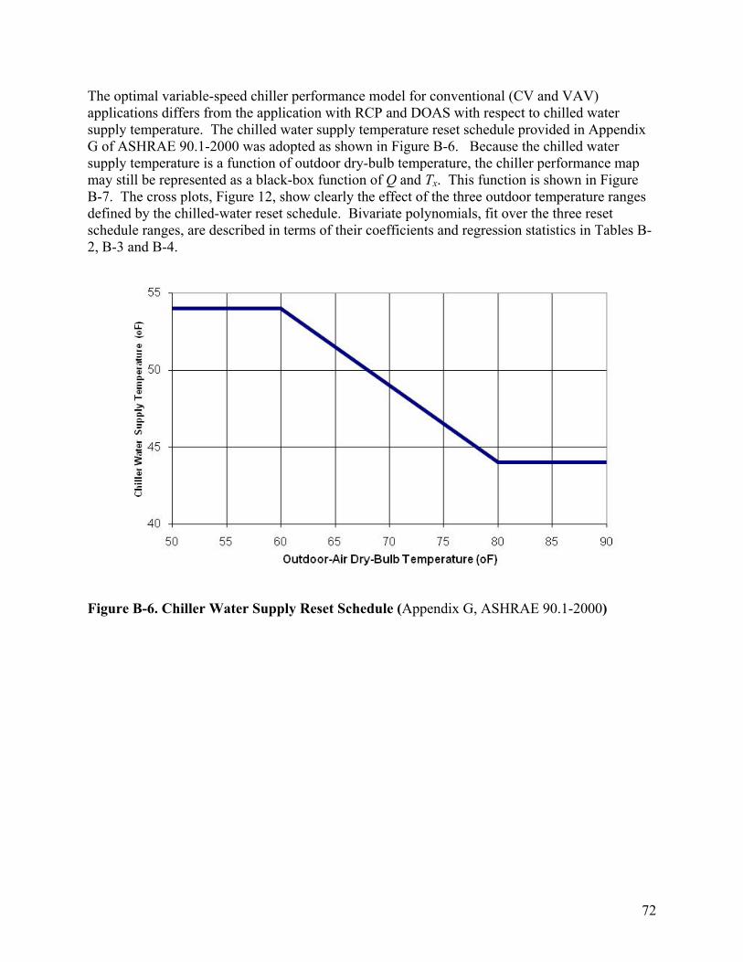
72

The optimal variable-speed chiller performance model for conventional (CV and VAV) applications differs from the application with RCP and DOAS with respect to chilled water supply temperature. The chilled water supply temperature reset schedule provided in Appendix G of ASHRAE 90.1-2000 was adopted as shown in Figure B-6. Because the chilled water supply temperature is a function of outdoor dry-bulb temperature, the chiller performance map may still be represented as a black-box function of Q and Tx. This function is shown in Figure B-7. The cross plots, Figure 12, show clearly the effect of the three outdoor temperature ranges defined by the chilled-water reset schedule. Bivariate polynomials, fit over the three reset schedule ranges, are described in terms of their coefficients and regression statistics in Tables B-2, B-3 and B-4.

Figure B-6. Chiller Water Supply Reset Schedule (Appendix G, ASHRAE 90.1-2000)

73

0 0.1 0.2 0.3 0.4 0.5 0.6 0.7 0.8 0.9 10

0.2

0.4

0.6

0.8

1

1.2

1.4S

peci

fic P

ower

(kW

/Ton

)

Part-Load Fraction

110100 90 80 70 60 50

Figure B-7. Chiller Map for the Chilled Water Reset Schedule Shown in Figure B-6 and Tx Ranging from 110°F to 50°F in 10°F Increments

50 60 70 80 90 100 1100

0.2

0.4

0.6

0.8

1

1.2

1.4

Spe

cific

Pow

er (k

W/T

on)

TODB (F)

6 9 12 18 24 30 36 45 60 75 90120150180210240270300

Figure B-8. Chiller Map Cross-plot for the Chilled Water Reset Schedule Shown in Figure B-6; Part Load Fraction Ranges Over 0.02:1.00 Applied to a 300kBh Nominal Capacity (B&W readers note: the legend is inverted; 300kBh is the top curve, 6kBh is the bottom).

74

Table B-2. Polynomial Performance Map (kW/Ton) for 50<T<60; x=Load Fraction, y=TODB (°F); r2=.9999

Term Coeff., C |C|/se const -8.240e-02 280.0

x 0 - y -2.986e-04 63.10 x2 3.986e-05 422.0 xy 2.378e-05 321.8 y2 -1.072e-06 53.12 x3 0 - x2y 0 - xy2 0 - y3 4.879e-09 108.1

Table B-3. Polynomial Performance Map (kW/Ton) for 60<TODB<80; x=Load Fraction, y=TODB (°F); r2=.9998


x 0 - y 9.030e-04 20.15 x2 5.647e-05 695.7 xy -3.757e-05 29.19 y2 1.098e-06 141.7 x3 0 - x2y 6.183e-07 67.24 xy2 0 - y3 0 -

Table B-4. Polynomial Performance Map (kW/Ton) for 80<TODB<110; x=Load Fraction, y=TODB (°F); r2=.9999


x 5.516e-03 1107. y 8.354e-04 33.44 x2 0 - xy -1.524e-05 29.11 y2 3.134e-06 114.6 x3 0 - x2y 3.139e-07 114.2 xy2 0 - y3 -4.409e-09 72.14

Hourly Cycling Performance of Two-Speed Chillers The 2-speed chiller is assumed to be identical to the variable speed chiller except that it can only operate at 0%, 50% and 100% of rated capacity. To satisfy a given hourly load, Q, with a

75

specified outdoor temperature, Tx, the 2-speed chiller must cycle on and off to satisfy an hourly load less than 50% of rated capacity, QDES, and it must cycle between low- and high-speed operation to satisfy an hourly load greater than 50% of rated capacity. The high-speed duty fraction is given as a function of X = Q/QDES by:

th = 2X – 1 (eqn. 27)

and since th < 0 implies X < 0.5, hourly performance may be evaluated as follows:

where f(Tx,X) is the chiller performance in Wh/Btu (1/EER) at outdoor temperature Tx and load fraction X. Note that Q, for fan systems during occupied hours, is the coil load after credit for air-side economizer capacity at prevailing return air and outdoor-air conditions.

Hourly Cycling Performance of Two-Speed Chiller in Unoccupied Hours

The lowest cost response to cooling demand in an unoccupied hour may entail running fans for less than the full hour. To determine the optimal response we first evaluate the low- and high-speed cooling capacities including economizer capacity, Qecon, and the corresponding values of specific power, R, including fan power, in Wh/Btu:

QL = 0.5QDES + Qecon; RL = Pfan + 0.5QDES f(Tx,0.5) (eqn. 28)

QH = QDES + Qecon; RH = Pfan + QDES f(Tx,1.0)) (eqn. 29)

where Qecon = Cfan(Tra – Tx) is the economizer capacity. The high-speed duty fraction is now

th = (Q – QL)/(QH – QL) which reduces to th = 2X – 1 when Qecon = 0. The algorithm must consider the possibility that the load may be satisfied more economically at high-speed than at low because low-speed chiller operation increases the duration of fan operation and associated fan energy is roughly doubled; conversely, if cooling is most efficiently provided by fan-only operation the chiller should be operated for the least possible fraction of the hour:

if (RH/QH) < (RL/QL) Esystem = (Q/QH)RH

elseif th < 0 if (Recon/Qecon) < (RL/QL);

else; Esystem = (Q/QL)RL else

Esystem = Q((1– th)RL/QL + th RH/QH) end

if th < 0 Echiller = Q f(Tx,0.5)

else Echiller = Q((1– th)f(Tx,0.5) + th f(Tx,1.0))

end

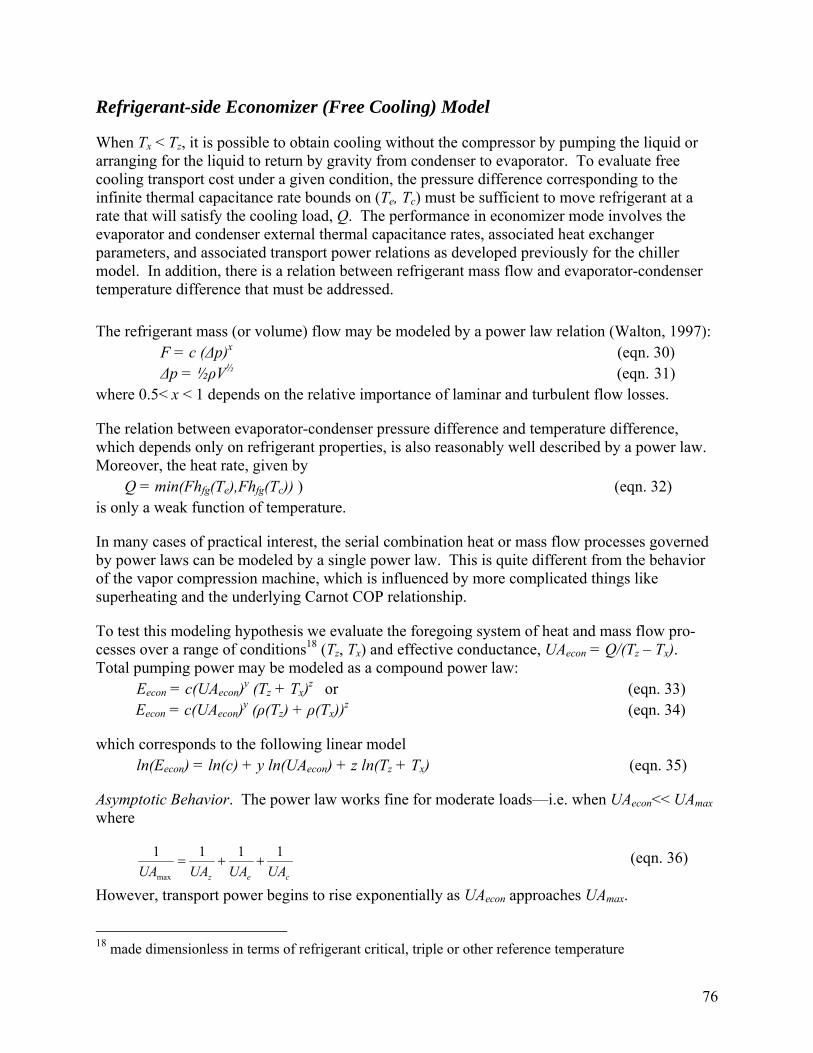
76

Refrigerant-side Economizer (Free Cooling) Model

When Tx < Tz, it is possible to obtain cooling without the compressor by pumping the liquid or arranging for the liquid to return by gravity from condenser to evaporator. To evaluate free cooling transport cost under a given condition, the pressure difference corresponding to the infinite thermal capacitance rate bounds on (Te, Tc) must be sufficient to move refrigerant at a rate that will satisfy the cooling load, Q. The performance in economizer mode involves the evaporator and condenser external thermal capacitance rates, associated heat exchanger parameters, and associated transport power relations as developed previously for the chiller model. In addition, there is a relation between refrigerant mass flow and evaporator-condenser temperature difference that must be addressed. The refrigerant mass (or volume) flow may be modeled by a power law relation (Walton, 1997): F = c (Δp)x (eqn. 30) Δp = ½ρV½ (eqn. 31)

where 0.5< x < 1 depends on the relative importance of laminar and turbulent flow losses.

The relation between evaporator-condenser pressure difference and temperature difference, which depends only on refrigerant properties, is also reasonably well described by a power law. Moreover, the heat rate, given by Q = min(Fhfg(Te),Fhfg(Tc)) ) (eqn. 32) is only a weak function of temperature.

In many cases of practical interest, the serial combination heat or mass flow processes governed by power laws can be modeled by a single power law. This is quite different from the behavior of the vapor compression machine, which is influenced by more complicated things like superheating and the underlying Carnot COP relationship.

To test this modeling hypothesis we evaluate the foregoing system of heat and mass flow pro-cesses over a range of conditions18 (Tz, Tx) and effective conductance, UAecon = Q/(Tz – Tx). Total pumping power may be modeled as a compound power law: Eecon = c(UAecon)y (Tz + Tx)z or (eqn. 33) Eecon = c(UAecon)y (ρ(Tz) + ρ(Tx))z (eqn. 34)

which corresponds to the following linear model ln(Eecon) = ln(c) + y ln(UAecon) + z ln(Tz + Tx) (eqn. 35)

Asymptotic Behavior. The power law works fine for moderate loads—i.e. when UAecon<< UAmax where

cez UAUAUAUA

1111

max

++= (eqn. 36)

However, transport power begins to rise exponentially as UAecon approaches UAmax.

18 made dimensionless in terms of refrigerant critical, triple or other reference temperature

77

We therefore augment the approximate model with a factor that mimics the observed behavior: Eecon = c(UAecon)y (Tz + Tx)z coth((UAmax–UAecon).5)18 (eqn. 37)

One might adjust the definition of UAmax as well to account for the effective reduction in Tz – Tx that corresponds to evaporator-condenser Δp near the UAmax (very high Ce and Cc) condition.

Map Generating Algorithm. Economizer performance at given UAecon, Tz and Tx is determined by a modified version of the chiller model that solves for the temperature, T, which minimizes transport power in economizer mode. First the saturated refrigerant properties, p, ρ and hfg, are evaluated at a feasible trial value of T, e.g.

T = (Re + Rc)(Tz/Re + Tx/Rc) (eqn. 38)

where Re = 1/UAe + 1/UAz and Rc = 1/UAc.

Next one must evaluate the mass flow rate needed to produce the required heat rate, Q: F = Q/hfg, (eqn. 39) and evaluate the pressure drop for F: Δp = (F/c)1/x (eqn. 40)

Evaporator and condenser pressures (p ± Δp/2) and the corresponding saturated temperatures are evaluated: Te = Tsat(p + Δp/2) (eqn. 41) Tc = Tsat(p – Δp/2) (eqn. 42)

and the thermal capacitance rates, Ce, Cc, and associated transport power requirements are evaluated using the heat exchanger solvers and flow power relations. We use the optimizer, fminbnd, to search on T for the minimum transport power. The optimizer executes the above evaluation steps for each new estimate of T until the sequence converges.

Second-Order Effects. The transport properties and refrigerant properties are functions of temperature. If UAmax is evaluated at a suitable mean temperature, the simplified model becomes invariant with respect to air and water conductivity temperature shifts (Prandtl and Nusselt moduli). The pumping power will still be very weakly sensitive to the Reynolds number transport properties of density and viscosity but this can be addressed by an external correction function.

The refrigerant properties present a more complicated picture. To assess the sensitivity we re-ran the mapper with a 20°F temperature shift affecting only the refrigerant properties. The differences in Log(transport power) are less than 0.01 for all cases in which transport power is less than 0.2 kW/Ton—i.e. for all conditions in which refrigerant-side free cooling is more efficient than running the compressor at very low speed.

A bivariate polynomial, fit over—and slightly beyond—the range of points where refrigerant-side economizer operation is more efficient than vapor-compression operation, is described in terms of its coefficients and regression statistics in Table B-5. In application, mode of operation is determined by evaluating both the vapor-compression and economizer-mode performance

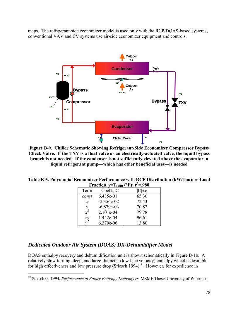
78

maps. The refrigerant-side economizer model is used only with the RCP/DOAS-based systems; conventional VAV and CV systems use air-side economizer equipment and controls.

Compressor

Condenser

Evaporator

TXV

Sight Glass

Outdoor Air

Outdoor Air

E1

E2

E3

T5

T6

T4

P1

P2

H3, T7

Chilled Water T2T3

F3

Bypass

BypassCompressor

Condenser

Evaporator

TXV

Sight Glass

Outdoor Air

Outdoor Air

E1

E2

E3

T5

T6

T4

P1

P2

H3, T7

Chilled Water T2T3

F3

Bypass

Bypass

Figure B-9. Chiller Schematic Showing Refrigerant-Side Economizer Compressor Bypass Check Valve. If the TXV is a float valve or an electrically-actuated valve, the liquid bypass branch is not needed. If the condenser is not sufficiently elevated above the evaporator, a

liquid refrigerant pump—which has other beneficial uses—is needed

Table B-5. Polynomial Economizer Performance with RCP Distribution (kW/Ton); x=Load Fraction, y=TODB (°F); r2=.988

Term Coeff., C |C|/se const 6.485e-01 65.36

x -2.356e-02 72.43 y -6.879e-03 70.82 x2 2.101e-04 79.78 xy 1.442e-04 96.61 y2 6.370e-06 13.80

Dedicated Outdoor Air System (DOAS) DX-Dehumidifier Model

DOAS enthalpy recovery and dehumidification unit is shown schematically in Figure B-10. A relatively slow turning, deep, and large-diameter (low face velocity) enthalpy wheel is desirable for high effectiveness and low pressure drop (Stiesch 1994)19. However, for expedience in 19 Stiesch G, 1994. Performance of Rotary Enthalpy Exchangers, MSME Thesis University of Wisconsin

79

scoping the annual energy benefits of LLC we have used the standard DOE-2.2 Energy and heat recovery ventilator (ERV) model and assume balanced20, constant air flow for the DOAS (implying constant occupancy or constant CO2 generation) during occupied hours21. For TOS configurations employing RCP/DOAS equipment the dehumidification section—here implemented as a variable-speed direct-expansion vapor compression machine—must satisfy the entire residual latent load, i.e. the total (building plus ventilation) latent load minus the latent cooling recovered by the enthalpy wheel. Constant volume operation, which is typical for DOAS, has three important advantages 1) fan and duct systems can be optimized considering operating and first costs in a straightforward way, 2) good ventilation efficiency can be achieved using simple, properly sized diffusers to introduce conditioned outside air to occupied spaces, and 3) demand-controlled ventilation, if used, can be simply implemented using on/off terminal dampers—in an office by a light switch position/occu-pancy sensor and in a large conference room by a CO2 sensor with duty-cycle control. In practical applications it is desirable that the supply air temperature be above the zone dew point (to prevent condensation on distribution ducts) and below about 80oF (to avoid discomfort). However, for this scoping study, we will reject all condenser heat back into the supply air stream thus adding to the sensible cooling load that the main chiller, TES (if present) and RCP distribution elements must remove22. The compressor in this application works against a moderate and fairly constant pressure ratio. The suction pressure is largely determined by the supply-air dew point needed to satisfy the latent load (50-55°F) and the discharge pressure with an exhaust-air auxiliary condenser will range between the return-air and outdoor-air dry-bulb temperatures.

20 Nearly balanced airflow—commonly assumed in the ERV performance analysis—requires a very tight building to maintain the small (10-20 Pa) positive building pressure considered desirable for air quality and control. Two factors make this a reasonable assumption 1) cost-effective low-leakiness technologies and commissioning methods already exist and 2) the economic, building code, and other policy positions that will encourage ZEB in general will inevitably promote substantially larger investments in the high-performance building envelope. 21In practice, some dehumidification might be used during unoccupied periods of pre-cooling. 22This approach has little effect on overall system efficiency but is sub-optimal in terms of first cost and could be problematic in terms of ventilation efficiency and comfort. To better address these costs and design issues, an exhaust-air-cooled auxiliary condenser downstream of the enthalpy wheel will be modeled in the next project stage and the desirability of supplementary evaporative cooling of the auxiliary condenser will be assessed. The cost and performance benefits of using a refrigerant mixture for temperature glide in (and associated low pressure ratio between) the evaporator and condenser(s) will also be assessed. Temperature glide is particularly advantageous for dehumidification because the condenser inlet and evaporator outlet air temperatures are equal and temperature glide can therefore reduce the pressure ratio substantially for a log(Pd/Ps) of perhaps half what can be achieved with a pure refrigerant. A reciprocating compressor is suitable but a specially designed (low-volume-index) scroll, vane type, or Roots (cycloidal rotor pair) compressor may be more efficient and cost-effective with temperature glide.

80

Com

pres

sor

Con

dens

er

Evap

orat

or

EXV

Outdoor Air

Supply Air

Exhaust Air

Return Air

Com

pres

sor

Con

dens

er

Evap

orat

or

EXV

Outdoor Air

Supply Air

Exhaust Air

Return Air

Figure B-10. Schematic of the DOAS Recovery and De-humidification System

Overview of the DX-Dehumidifier. The dehumidifier performance can be addressed with separate models for the compressor-condenser and DX evaporator coil. For a given airflow rate, inlet temperature and total load, QDX = QL + QS = mSA(hDXINLET – hSA), the refrigerant saturation temperature, TSS, is strictly increasing with latent load fraction, QL/QDX. Under conditions that would result in a partially wetted evaporator coil, models that assume fully wetted or completely dry air-side surfaces return TSS estimates lower than would be returned by a model with separate dry- and wet-surface sub-models. However, the wet-surface model estimate of TSS is generally close to the actual value when any fraction of the coil is wetted (Braun, 1989c; Reichler, 1999) and in this application part of the coil is always wet. Thus the fully-wetted assumption results in a simple analysis that gives a conservative EER. With the series evaporator-condenser arrangement of interest, the error in TSS resulting from the fully-wetted assumption is relatively small compared to the total lift, (Tc-TSS), over a wide range of inlet conditions23 and the error in EER stemming from this assumption will be similarly small24. Having evaluated TSS and leaving air temperature (evaporator leaving air temperature is exactly the condenser entering air temperature), we can compute the compressor speed and power needed to just satisfy evaporator load with the airflow rate, Cair, required for ventilation in a given hour. The compressor and condenser sub-models, introduced previously in connection with generating a chiller performance map, are used with a DOAS-specific set of equipment parameters to solve for the refrigerant condensing temperature, Tc. Note that in this case there is no need to pre-compute a performance map because performance of the DX-dehumidifier is evaluated at most once for each hour in which there is a latent cooling load; dehumidifier operation is not involved in or affected by the load shifting optimization process. Excessive reheat (beyond zone set-point) of supply air by the condenser is permitted; this is equivalent to rejecting balance of condenser heat to the main chiller or, with TES in play, to 23Lift and Te error increase together as sensible heat ratio increases, therefore EER error is approximately constant 24A partly wetted coil and refrigerant temperature glide will be modeled in Phase-2 work.

81

rejecting the balance of condenser heat to TES. Thus the DOAS (ERV and DX dehumidifier) is evaluated each hour to determine the additional sensible load, if any, to be added to the building’s instantaneous sensible cooling load; this is done before and independent of any chiller-TES load shifting optimization25. The heat wheel analysis is straightforward given airflow (same for supply and return), and known inlet temperatures: TRA = Tzone on the return side and TINLET mainly a function of QDX on the supply side. The dehumidifier performance is addressed in two steps. The evaporator temperature, TSS , is first computed independently based on coil load, QDX, and inlet (TINLET, hINLET) conditions. Given QDX and TSS, the compressor-condenser model can then solve for Tc with compressor speed and refrigerant flow as intermediate variables. Compressor power is evaluated after solving for Tc by evaluating the semi-empirical compressor power sub-model that takes Tc, TSS, refrigerant mass flow rate, and shaft speed as inputs.

Derivation of DX Coil Model The DX coil model determines refrigerant evaporating temperature, TSS, given load and entering air Tw.. For a dry DX coil there is only sensible cooling and local heat transfer rate is given by

dQ = U(Tair - TSS)dA (eqn. 43) where U = air-to-water side thermal conductance per unit area26, dA = differential area along the air-side path (from air-side inlet to outlet), TSS = refrigerant-side saturated suction (evaporating) temperature, and Tair = temperature of process air, a function of position on the air-side path.

The infinite-NTU DX dry-coil capacity is Qmax = Cair(TairINLET - TSS) (eqn. 44)

and the effectiveness-NTU model can be used to estimate actual coil capacity as follows

Q = εCair(TairINLET - TSS) (eqn. 45) where

ε = 1 – e-NTU (eqn. 46) Cair = air-side thermal capacitance rate, and

NTU = UA/Cair (eqn. 47) The overall conductance is often approximated by assuming that the heat transfer rate is controlled by the air and refrigerant side resistances which are uniform over part or all of the heat exchanger, thus:

25 Or it could be considered a non-shiftable part of the load. 26 although any consistent (UA = ∫U dA) basis may be used, this is usually taken to be the refrigerant inside tube surface area.

82

rair hAhA

UA

)(1

)(1

1

+≅ (eqn. 48)

where (hA)air = air-side conductance and (hA)r = refrigerant-side conductance

The air-side process with high latent load (fully wetted DX coil) is actually a combined mass and thermal diffusion process driven by a temperature gradient and a moisture gradient. The gradients are not independent but are linked through the moist air properties. Thus the two gradients may be modeled approximately by a single enthalpy gradient and the wetted-coil local heat transfer analogy is: dQ = Ud(hair - hs)dA (eqn. 49) where Ud = effective enthalpy conductance, hs = enthalpy of saturated air evaluated at refrigerant-side evaporating temperature, hair = enthalpy of process air, a function of position on the air-side path, and dA = differential area along the air-side path (from air-side inlet to outlet). The maximum possible wet DX coil capacity using the thermal diffusion analogy is Qmax = mair(hairINLET - he) (eqn. 50) and the effectiveness-NTU model estimates actual wetted coil capacity as follows Q = εhmair(hairINLET - he) (eqn. 51) where

εh = 1 – exp(-NTUh) (eqn. 52) mair = air-side mass flow rate, and NTUh = UAh/mair (eqn. 53)

The enthalpy diffusion conductance is approximated by defining equivalent air-side and equivalent refrigerant-side resistance for combine heat and moisture diffusion, thus:

r

s

air

airph

hAc

hAcUA

)()(

1, +

≅ (eqn. 54)

where

sw

swsat

SSINLETdp

SSsatINLETdpsats dT

TdhTT

ThThc )()()(

,

, ≈−

−≈ (eqn. 55)

Tdp,INLET = entering air dew point temperature and Tsw = average temperature of wetted surface.

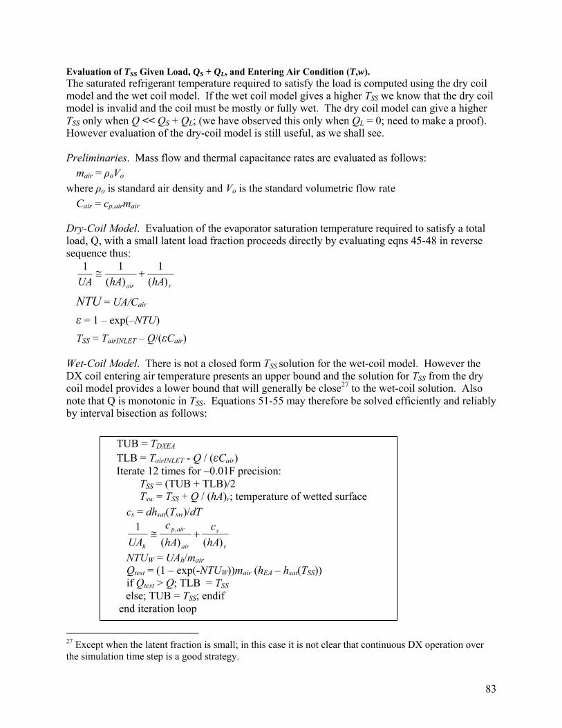
83

Evaluation of TSS Given Load, QS + QL, and Entering Air Condition (T,w). The saturated refrigerant temperature required to satisfy the load is computed using the dry coil model and the wet coil model. If the wet coil model gives a higher TSS we know that the dry coil model is invalid and the coil must be mostly or fully wet. The dry coil model can give a higher TSS only when Q << QS + QL; (we have observed this only when QL = 0; need to make a proof). However evaluation of the dry-coil model is still useful, as we shall see. Preliminaries. Mass flow and thermal capacitance rates are evaluated as follows:

mair = ρoVo where ρo is standard air density and Vo is the standard volumetric flow rate

Cair = cp,airmair Dry-Coil Model. Evaluation of the evaporator saturation temperature required to satisfy a total load, Q, with a small latent load fraction proceeds directly by evaluating eqns 45-48 in reverse sequence thus:

rair hAhAUA )(1

)(11

+≅

NTU = UA/Cair

ε = 1 – exp(–NTU)

TSS = TairINLET – Q/(εCair)

Wet-Coil Model. There is not a closed form TSS solution for the wet-coil model. However the DX coil entering air temperature presents an upper bound and the solution for TSS from the dry coil model provides a lower bound that will generally be close27 to the wet-coil solution. Also note that Q is monotonic in TSS. Equations 51-55 may therefore be solved efficiently and reliably by interval bisection as follows:

27 Except when the latent fraction is small; in this case it is not clear that continuous DX operation over the simulation time step is a good strategy.

TUB = TDXEA

TLB = TairINLET - Q / (εCair) Iterate 12 times for ~0.01F precision: TSS = (TUB + TLB)/2 Tsw = TSS + Q / (hA)r; temperature of wetted surface

cs = dhsat(Tsw)/dT

r

s

air

airp

h hAc

hAc

UA )()(1 , +≅

NTUW = UAh/mair Qtest = (1 – exp(-NTUW))mair (hEA – hsat(TSS)) if Qtest > Q; TLB = TSS

else; TUB = TSS; endif end iteration loop

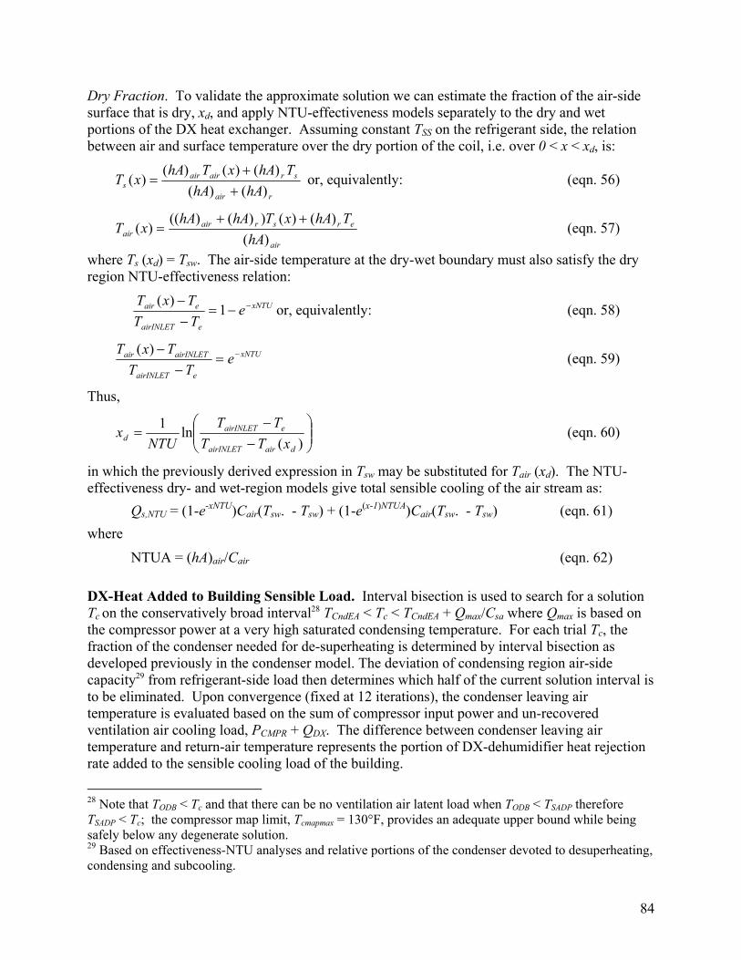
84

Dry Fraction. To validate the approximate solution we can estimate the fraction of the air-side surface that is dry, xd, and apply NTU-effectiveness models separately to the dry and wet portions of the DX heat exchanger. Assuming constant TSS on the refrigerant side, the relation between air and surface temperature over the dry portion of the coil, i.e. over 0 < x < xd, is:

rair

srairairs hAhA

ThAxThAxT

)()()()()(

)(++

= or, equivalently: (eqn. 56)

air

ersrairair hA

ThAxThAhAxT

)()()())()((

)(++

= (eqn. 57)

where Ts (xd) = Tsw. The air-side temperature at the dry-wet boundary must also satisfy the dry region NTU-effectiveness relation:

xNTU

eairINLET

eair eTTTxT −−=−−

1)(

or, equivalently: (eqn. 58)

xNTU

eairINLET

airINLETair eTT

TxT −=−

−)( (eqn. 59)

Thus,

⎟⎟⎠

⎞⎜⎜⎝

⎛−

−=

)(ln1

dairairINLET

eairINLETd xTT

TTNTU

x (eqn. 60)

in which the previously derived expression in Tsw may be substituted for Tair (xd). The NTU-effectiveness dry- and wet-region models give total sensible cooling of the air stream as:

Qs,NTU = (1-e-xNTU)Cair(Tsw. - Tsw) + (1-e(x-1)NTUA)Cair(Tsw. - Tsw) (eqn. 61) where

NTUA = (hA)air/Cair (eqn. 62) DX-Heat Added to Building Sensible Load. Interval bisection is used to search for a solution Tc on the conservatively broad interval28 TCndEA < Tc < TCndEA + Qmax/Csa where Qmax is based on the compressor power at a very high saturated condensing temperature. For each trial Tc, the fraction of the condenser needed for de-superheating is determined by interval bisection as developed previously in the condenser model. The deviation of condensing region air-side capacity29 from refrigerant-side load then determines which half of the current solution interval is to be eliminated. Upon convergence (fixed at 12 iterations), the condenser leaving air temperature is evaluated based on the sum of compressor input power and un-recovered ventilation air cooling load, PCMPR + QDX. The difference between condenser leaving air temperature and return-air temperature represents the portion of DX-dehumidifier heat rejection rate added to the sensible cooling load of the building.

28 Note that TODB < Tc and that there can be no ventilation air latent load when TODB < TSADP therefore TSADP < Tc; the compressor map limit, Tcmapmax = 130°F, provides an adequate upper bound while being safely below any degenerate solution. 29 Based on effectiveness-NTU analyses and relative portions of the condenser devoted to desuperheating, condensing and subcooling.

85

Appendix B References

1. Braun, J, SA Klein and JW Mitchell. 1989. Effectiveness models for cooling towers and cooling coils. ASHRAE Trans. 95(2): 164-174.

2. Conroy, C.L., S.A. Mumma, 2001. Ceiling radiant cooling panels as a viable distributed parallel sensible cooling technology integrated with dedicated outdoor-air systems. ASHRAE Trans. 107(1).

3. Hiller, Carl C., 1976. Improving Heat Pump Performance via Compressor Capacity Control, MIT Dept. Mechanical Engineering, PhD Thesis

4. King, D.J. and R.A. Potter, 1998. Description of a steady-state cooling plant model developed for use in evaluating optimal control of ice thermal energy storage systems, ASHRAE Trans. 104(1A)42-53

5. National Institute of Standards and Technology. 2007. Standard Reference Database 23 - NIST Reference Fluid Thermodynamic and Transport Properties Database (REFPROP 7.0). http://www.nist.gov/srd/nist23.htm.

6. Gordon, J.M. and K.C. Ng, 2000. Cool Thermodynamics, Cambridge Int’l Science Publishing.

7. Rabehl, R.J., J.W. Mitchell and W.A. Beckman, Parameter estimation and the use of catalog data in modeling heat exchangers and coils. HVAC&R Res. 5 1 (1999), pp. 3–17.

8. Reichler, Mark 1999. Modeling of Rooftop Packaged A/C Equipment, MSME UW Madison. minds.wisconsin.edu/bitstream/1793/7672/1/Thesis.pdf

9. Stiesch, G., (UW-SEL M.S., 1994), Performance of Rotary Enthalpy Exchangers http://sel.me.wisc.edu/theses/Stiesch.zip

10. Threlkeld, J.L., 1970. Thermal Environmental Engineering, 2nd edtn., Prentice-Hall, Englewood Cliffs, NJ; see also Keuhn, T.H., et al, 1998, 3rd edtn.

11. Walton, G.N. 1997. CONTAM96--User Manual, NISTIR 5385. Gaithersburg: National Institute of Standards and Technology.

86

Appendix C. Modeling and Analysis Assumptions

87

Appendix C. Modeling and Analysis Assumptions In this Appendix, assumptions made in the development of component models and annual energy use estimates for the various TOS and medium-office building configurations are documented. The basis or justification is given for key assumptions in terms of project scope and resources and the current state of modeling capabilities and sources of primary information.

• A lossless and perfectly stratified ideal storage was assumed for TES cases. This assumption is optimistic, but not overly so, for the high-performance building (even in perimeter zones) in which both internal-gain and solar cooling loads are low and there is thus sufficient intrinsic thermal capacitance in the building fabric (passive thermal storage) to satisfy the peak diurnal cooling load with acceptable room temperature excursions. Actual energy use will be higher, in practice, to the extent that envelope losses increase with Tx - Tz, because lower values of Tz are inevitable during precooling.

• Omniscient control. The 24-hour weather and internal gain forecasts are assumed to be perfectly accurate so that storage is never overcharged. In a practical installation the forecasts will be continuously updated so the effect of weather uncertainty should be small. The effect of internal gain uncertainty can be assessed to some extent in the next phase of the work (FY08) but cannot be fully assessed until more primary data on internal load variability has been collected or existing time series data is made available for uncertainty analysis.

• TES carryover beyond each 24-hour control period is constrained to be zero. By not

admitting carryover, the results are somewhat conservative for discrete storage and representative of savings that might be expected with passive (intrinsic mass) storage for cases where total daily load can be stored with acceptable room temperature excursions.

• Night cooling is optimized on the basis of a constant price for electricity for two reasons:

the project objective is energy efficiency rather than cost and the advent of site-generated power will modify the supply cost picture in unforeseeable ways as on-site generation and end-user load-shifting technologies evolve. The integration of photovoltaic on-site generation with the TOS is a topic of intense interest for phase-2 work.

• The zone temperature set point schedule is assumed the same for all building configurations and all configurations provide equivalent thermal comfort and outside ventilation air-change rates.

• Return air temperature and humidity equal to zone temperature and humidity, i.e., assume no return duct loss or gain between the zone and the return side of the DOAS subsystem.

• Extra pumping energy (for cooling from storage) is not accounted for in the TES cases because the preferred implementation—intrinsic TES—does not require extra pumping and for discrete TES this is generally a small fraction of annual chiller input energy.

• All chiller configurations use the flooded-evaporator arrangement typical of large

chillers. The flooded evaporator is a key element of low-lift chiller design; by making

88

this assumption for all configurations, including the baseline, the performance improvements for the TOS and partial TOS cases are conservative. Further evaluation of the effect of suction superheat on annual performance can be made in the next phase.

• All chiller configurations are sized the same because a procedure for optimal sizing needs

detailed cost information that will not be available until the next phase. Even if it is determined that the most cost-effective designs with TES use a smaller chiller, designers may be reluctant to specify a chiller than cannot satisfy the peak load without storage.

• Performance of 1- and 2-speed chiller configurations are taken from the 50% and 100%

part-load points of the variable-speed chiller performance maps to ensure comparability of the configurations in the most straightforward and defensible manner. This assumption is optimistic for 1- and 2-speed configurations because the fan, pump and compressor speeds are made to vary such that input power is minimized at any given outdoor dry-bulb temperature. The effect is small for well-designed unitary air-conditioning equipment or small chillers but may be significant for mid-market equipment that has been "designed to the EER rating condition," e.g., it is common practice to employ a condenser 2-fan sequence that is wasteful in terms of transport efficiency when only one fan is running.

• For the chiller performance maps with specified chilled water supply temperature the

performance is slightly affected by chilled-water return temperature which, for fan-coil (CV or VAV) systems, is affected by mixed-air conditions. We assume that the ASHRAE chilled water reset schedule results in coil sensible heat ratio (SHR) reasonably close to actual load SHR and that the mixed air temperature equals the occupied-period zone set point.

• The variable speed drive (VSD) compressor is assumed to operate reliably with respect to motor cooling and lubrication over a wide speed range of 20:1. Reciprocating, scroll and rolling piston compressors in engine-driven as well as stationary motor driven compressor applications typically modulate over a 4:1 speed range. The wider speed range can be achieved by modification of oil pump and oil return mechanisms or by using two compressors sized for 0.2 and 0.8 of total capacity and each operating over the conservative 4:1 speed range.

• The variable-speed condenser fan and chilled water transport models are based on

standard power-flow relations in which an essentially constant combined mechanical and electrical efficiency is implicit. Two-speed chiller operating points are taken from the corresponding variable-speed chiller map and hence reflect the same assumed power-flow relations.

• Although a number of refrigerants are suitable to be used with the TOS, only R-22

refrigerant based systems were modeled for this effort. In the next phase, other non-CFC based refrigerants, including zeotropic mixtures, will be considered for the TOS.

89

• For the fan coil (CV or VAV) configurations a larger than normal UA was specified to compensate for not modeling wet-coil enthalpy transfer.

• In generating the chiller performance maps the heat exchanger capacities have been modeled by standard NTU-effectiveness relations but the conductances (numerator of NTU) have been assumed to be constant. In the next phase, heat exchanger models will be refined to reflect typical variation of conductance with air- water- and refrigerant-side flow rates.

• The enthalpy recovery wheel is modeled by DOE-2.2 as having constant effectiveness for

heat and mass transfer.

• Savings attributable to the RCP/DOAS system’s ability to heat and cool during unoccupied hours without fan operation, hence without the penalty of outside air damper leakage and duct losses, was not analyzed. This is somewhat optimistic for fan systems especially when the chiller is run at night for pre-cooling (TES cases).

• A variable-speed DX-dehumidifier was used for all RCP/DOAS configurations

regardless of the main chiller configuration (2-speed or variable-speed low-lift).

• All heat rejected by the DX-dehumidifier is rejected to the supply air stream and thus added to the sensible cooling load imposed on the main chiller. In a practical system some or all of the heat would be rejected to the exhaust air stream or directly to the outside air. The system performance impacts of these and other (e.g. evaporative cooling using water removed from the supply air-stream by the evaporator) heat rejection schemes can be assessed in the next phase.

• Although parts of the TOS can provide heating energy savings, only cooling energy

savings are computed in the analysis. Radiant heating generally results in equivalent comfort with lower room air temperatures and correspondingly lower conduction and infiltration heat losses. In addition, some configurations (Cases) may have re-heating penalties, which have not been analyzed. Omission of these two heating and cooling load reducing mechanisms lead to conservative estimates of the technical energy savings potential.

• The baseline, medium-performance, and high-performance buildings were not modeled

to use daylighting controls primarily because the AEDG prototype was not designed to make good use of daylighting potential. Phase-2 work should include a subtask to inves-tigate daylighting versus efficient cooling tradeoffs because the high cooling efficiency afforded by the low-lift TOS may make more aggressive use of daylighting cost effective.

cost-effective integration of efficient low-lift base … · cost-effective integration of...

Documents