correlations in complex networks - physcomp2 ::: physics and
TRANSCRIPT

June 6, 2007 9:49 WSPC/Trim Size: 9in x 6in for Review Volume book
CHAPTER 3
Correlations in Complex Networks
M. Angeles Serrano1, Marian Boguna2, Romualdo Pastor-Satorras3 andAlessandro Vespignani1
1 School of Informatics and Biocomplexity Institute, Indiana University,Eigenmann Hall, 1900 East Tenth Street, Bloomington, IN 47406, USA
2 Departament de Fisica Fonamental, Universitat de Barcelona,Marti i Franques 1, 08028 Barcelona, Spain
3 Departament de Fisica i Enginyeria Nuclear, Universitat Politecnica deCatalunya, Campus Nord B4, 08034 Barcelona, Spain
3.1. Introduction
Most real networks exhibit the presence of non trivial correlations in theirconnectivity pattern. Indeed, empirical measurements bring evidence to thefact that, in some instances, high or low degree vertices of the network tendto preferentially connect to other vertices with similar degree. In this situa-tion, correlations are named assortative and are typically observed in socialnetworks.41 On the other hand, connections in many technological and bi-ological networks42 attach vertices of very different degree with strongerlikelihood. Correlations are in this case referred to as disassortative. Theoverall origin of the appearance of these correlations is not yet completelyunderstood, neither is the reason for the distinction in real systems betweenassortative and disassortative behavior. Correlations, however, drasticallyimpact the topological properties of networks, encoding the blueprint ofstructural organization and are customarily used as a method to classifyreal nets. Moreover, correlations do not only have a topological relevancebut may impact a variety of related problems such as percolation phe-nomena, resilience and robustness, spreading processes, or communicationefficiency, to name just a few. For these reasons, several strategies have beenproposed to model correlated networks. The most general practical algo-
35
June 6, 2007 9:49 WSPC/Trim Size: 9in x 6in for Review Volume book
36 M. A. Serrano, M. Boguna, R. Pastor-Satorras and A. Vespignani
rithms allow the construction of networks matching any desired correlationpattern. Other just generate correlations of a fixed signature.
In the following sections, we will focus on the characterization and mod-eling of correlations in undirected unweighted complex networks. In partic-ular, we will devote our attention to the statistical characterization of thesefeatures in large scale networks. In the section, we review some importantand useful general analytical results concerning the topological character-ization of random networks. In the third section we recall a number ofspecific metrics. In particular, two vertices correlations will be character-ized by the average degree of nearest neighbors as a function of the vertexdegree, knn(k), and correlations among three vertices will be described byseveral clustering measures, in particular the average clustering coefficientfor vertices of a given degree c(k). Real networks are discussed in the fourthsection, where we present some well-known and representative examples ofcorrelated structures, such as the science collaboration network of physi-cists submitting papers to a preprint database, the Pretty-Good-Privacyweb of trust between users of digital communications, the world-wide airtransportation network (all of them assortative), and the Internet at theAutonomous System level, the protein interaction network of the yeast S.Cerevisiae, and the world trade web of commercial exchanges between coun-tries in the world (all of them disassortative). Finally, recent developmentsin the modeling of correlated networks will be discussed in the fifth section.We distinguish between disassortative correlations, derived as an implicitconsequence from the formulation of some classical models, and assortativecorrelations which should be specifically introduced in theoretical construc-tions. Several more general and rigorous frameworks able to reconstruct awide range of correlation patterns are also presented. Finally, we concludeby providing an outlook on current and future developments.
3.2. Detailed balance condition
Although several possibilities could be considered, the conditional prob-abilities P (k′, k′′, . . . , k(n) | k) that a vertex of degree k is simultaneouslyconnected to a number n of other vertices with corresponding degreesk′,k′′,. . . ,k(n) might be the simplest theoretical functions that encode de-gree correlation information from a local perspective. A network is said tobe uncorrelated when the conditionality on k does not apply and, therefore,the only relevant function is just the degree distribution P (k). Otherwise,P (k) cannot be considered in isolation and degree correlations must be

June 6, 2007 9:49 WSPC/Trim Size: 9in x 6in for Review Volume book
Correlations in Complex Networks 37
taken into account through the conditional probability functions up to thepertinent order. In particular, two vertices and three vertices degree cor-relations are respectively encoded by the conditional probabilities P (k′ | k)and P (k′, k′′ | k).
Due to the fact that edges join pairs of nodes, the key functions at thelowest level are P (k) and P (k′ | k). Theoretically, they can have any formwith only two constraints. First, they must be normalized, i.e.∑
k
P (k) =∑k′
P (k′ | k) = 1. (33)
Second, all edges must point from one vertex to another, so that no edgeswith dangling ends exist in the network. Thus, the total number of edgespointing from vertices of degree k to vertices of degree k′ must be equalto the number of edges that point from vertices of degree k′ to verticesof degree k. In other words, these functions must obey a degree detailedbalance condition:43
kP (k′|k)P (k) = k′P (k|k′)P (k′), (34)
stating the closure of the network through the physical conservation ofedges among vertices. To prove this condition, we will follow an intuitivederivation.44
Let Nk be the number of vertices of degree k, so that∑
k Nk = N , whereN is the total number of nodes in the network. In the thermodynamic limit,we can calculate the degree distribution as a frequency distributiond, thatis,
P (k) ≡ limN→∞
Nk
N. (35)
Additionally, to complete the topological characterization of the network,we need also to specify how the different degree classes are connected to eachother. To this end, let us consider the symmetric matrix Ekk′ accountingfor the total number of edges between vertices of degree k and vertices ofdegree k′ for k �= k′. The diagonal values Ekk are equal to two times thenumber of connections between vertices in the same degree class, k = k′.This matrix meets the following identities:∑
k′Ekk′ = kNk, (36)∑
k,k′Ekk′ = 〈k〉N = 2E, (37)
dFor the sake of simplicity, in what follows we will obviate the limit.

June 6, 2007 9:49 WSPC/Trim Size: 9in x 6in for Review Volume book
38 M. A. Serrano, M. Boguna, R. Pastor-Satorras and A. Vespignani
where 〈k〉 is the average degree and E is the total number of edges in thenetwork. The first identity simply states that the total number of edgesemanating from vertices of degree k is k times the number of vertices inthis degree class. The second identity just states that the sum of the degreesof all nodes in the network is equal to two times the number of edges.
The first identity allows to write the conditional probability as
P (k′ | k) =Ek′k
kNk. (38)
On the other hand, from the second identity we can define the joint degreedistribution as
P (k, k′) =Ekk′
〈k〉N , (39)
where the symmetric function (2−δk,k′)P (k, k′) is equal to the probabilitythat a randomly chosen edge connects two vertices of degrees k and k′. Theconditional probability can be easily related to the joint degree distribution,namely
P (k′ | k) =〈k〉P (k, k′)
kP (k). (40)
The symmetry of P (k, k′) leads directly from the previous equation tothe detailed balance condition:
kP (k′ | k)P (k) = k′P (k | k′)P (k′) = 〈k〉P (k, k′). (41)
The pre-factors k and k′ in this equation account for the multiplicativenature of networks as random processes and the whole relation stands asthe closure condition for networks with no detached edge ends and withno isolated vertices. On the technical side, the detailed balance conditionconstraints the possible form of the conditional probability P (k′ | k) onceP (k) is given, and vice versa.
Making use of this important relation and the normalization condition,P (k) can also be written as a function of the joint degree distributione:
P (k) =〈k〉k
∑k′
P (k, k′). (42)
Among all the networks one can consider, Markovian networks are par-ticularly important.43 This class of network is completely defined by its
eNotice that this relation excludes vertices of degree 0, which are never considered inreal complex networks.

June 6, 2007 9:49 WSPC/Trim Size: 9in x 6in for Review Volume book
Correlations in Complex Networks 39
degree distribution P (k) and the first conditional probability P (k′|k). Inother words, such networks belong to a statistical ensemble which is max-imally random under the constraint of having a given degree distributionand a given first conditional probability. In this case, the joint distribu-tion P (k, k′) conveys all the relevant topological information since bothP (k) and P (k′|k) can be derived from it. In turn, all higher-order correla-tions can also be expressed as a function of these fundamental functions.In particular, the three vertices conditional probability can be written asP (k′, k′′|k) = P (k′|k)P (k′′|k) and the same applies to higher order correla-tion functions.
The meaning of the term Markovian network that we use in this chapteris borrowed from the theory of Stochastic Processes. In this field, a stochas-tic process X(t) is called Markovian if the probability to find the processat the position X(t) = x at time t only depends on its position at theprevious time t′ < t. Then, the process is completely characterized by theprobability density function p(x, t) of being at x at time t and the transitionprobability density p(x, t|x′, t′) of being at x at time t, provided that theprocess was at x′ at time t′. If we identify P (k) with p(x, t) and P (k′|k)with p(x, t|x′, t′), we can define Markovian networks in a similar manner.One can force even more the analogy and find another connection betweenMarkovian networks and Markovian stochastic processes. Suppose, for in-stance, a particle that randomly diffuses through the network, uniformlychoosing at each time step one of its neighbors to continue its walk. If theunderlying network is Markovian, the stochastic process constructed fromthe sequence of degrees of the visited vertices follows a Markovian jumpprocess with a transition probability given by P (k|k′) and a steady statedistribution given by kP (k)/〈k〉. Notice that the meaning of Markoviannetwork should not be confused with the notion of Markov graph.45
3.3. Empirical measurement of correlations
At the level of two vertices degree correlations, the most straightforwardmeasure consists in a direct inspection of the two-dimensional histogramsof the joint degree distribution P (k′, k)46,47 or the conditional probabilityP (k′ | k). However, such histograms in finite size systems are highly affectedby statistical fluctuations and are thus not good candidates to evaluate em-pirical correlations. In order to characterize degree correlations, it is thenmore convenient to adopt other standards, which nevertheless will eventu-ally depend on these functions. A most useful approach consists in defining

June 6, 2007 9:49 WSPC/Trim Size: 9in x 6in for Review Volume book
40 M. A. Serrano, M. Boguna, R. Pastor-Satorras and A. Vespignani
a one-parameter function encoding the signature of correlations. In the caseof two vertices correlations, such function is defined as the average nearestneighbors degree (ANND) of nodes with degree k, knn(k).48 It considersthe mean degree of the neighbors of a vertex as a function of its degree k.When this function increases with k, the network is named assortative, withvertices associating preferentially to other vertices of similar degree. Whenknn(k) instead decreases, the network is named disassortative, with high-degree vertices attaching preferentially to other low-degree ones. Hence, thisis a representation which gives a clear interpretation of pair correlations andat the same time can provide further information about hierarchical orga-nization in networks. Finally, the scalar Pearson correlation coefficient ofthe degrees of vertices at the ends of edges is used to summarize the levelof correlation with a single numberf .41,42
Despite the increasing attention in the literature about the measurementof P (k′, k), the first correlation observable appearing in the literature is thenetwork transitivity or clustering coefficient,6,7 a scalar which quantifies theprobability that two vertices with a common neighbor are also connected toeach other. This concept has its roots in sociology and, in the language ofsocial networks, it measures the likelihood that the friend of your friend isalso your friend. Therefore, it is in fact a measure of three vertices correla-tions although, curiously, it is among the first studied structural propertiesof networks, together with the small-world effect or the degree distribution.This definition and other alternatives49,50 have been broadly used to quan-tify in a statistical sense the deviation of real networks, strongly clustered,from the behavior of classical random graphs.
Since clustering measures triangles in a network, it seems also natural topose the question of how to measure higher order loops (closed paths). Thisissue is particularly important in order to asses if a network can be assumedto be Markovian, since, in this case, the loop structure must be very welldescribed by the two vertices correlations. A number of authors have paidattention to loops of length four and above. However, there are technicaldifficulties when one tries to separate the independent contributions of thedifferent motifs.51–55 This is the main reason why triangles –and not higherorder loops– have been chosen as a measure of correlations.
In this section we will concentrate on the broadly accepted and usedstatistical correlation observables in the analysis of large scale networks,
fThe Pearson coefficient is computed as the correlation coefficient of the joint distributionP (k, k′).

June 6, 2007 9:49 WSPC/Trim Size: 9in x 6in for Review Volume book
Correlations in Complex Networks 41
the average nearest neighbors degree and the degree dependent clusteringcoefficient, focusing on their theoretical grounds and significance.
3.3.1. Two vertices correlations: ANND
The average nearest neighbors degree, knn(k), of vertices of degree k isdefined as a smoothed conditional probability:48
knn(k) =∑k′
k′P (k′ | k), (43)
so that the statistical fluctuations that usually disturb the evaluation ofP (k′ | k) are damped.
Real networks usually tend to display one of two different patterns:either knn(k) is a monotonous increasing function of k or, on the contrary,it is a monotonous decreasing function of k. At the level of correlationproperties, this segregation allows the classification of networks based ontheir ANND behavior:41
• Assortative networks exhibit knn(k) functions increasing with k,which denotes that vertices are preferentially connected to othervertices with similar degree. Examples of assortative behavior aretypically found in many social structures.
• Disassortative networks exhibit knn(k) functions decreasing withk, which implies that vertices are preferentially connected to othervertices with very different degree. Examples of disassortative be-havior are typically found in several technological networks, as wellas in communication and biological networks.
This measure provides a sharp evidence for the presence or absenceof correlations since, in the case of uncorrelated networks, it is easy todemonstrate that this quantity should not depend on k. In fact, the un-correlated ANND value is found to coincide with the heuristic parameterκ = 〈k2〉/〈k〉, independently introduced to characterize the level of het-erogeneity of networks.12 For homogeneous networks κ ∼ 〈k〉, whereas forscale-free (SF) networks with unbounded degree fluctuations it diverges inthe thermodynamic limit. As a consequence, it comes to be a key parametercharacterizing the properties of networks and the processes running on topof them.
Here, we deduce kuncnn (k) from the detailed balance and the normaliza-
tion conditions. Summing Eq. 41 over k and recalling that Punc(k′|k) does
June 6, 2007 9:49 WSPC/Trim Size: 9in x 6in for Review Volume book
42 M. A. Serrano, M. Boguna, R. Pastor-Satorras and A. Vespignani
not depend on this variable, we obtain that
Punc(k′|k) =k′P (k′)〈k〉 , (44)
from where we have
kuncnn (k) =
〈k2〉〈k〉 . (45)
Therefore, a function knn(k) showing any explicit dependence on k signalsthe presence of degree correlations in the system.
As in the case of uncorrelated networks, it is also possible to derive somegeneral exact results concerning the behavior of knn(k) in the case of SFnetworks with a degree distribution of the form P (k) ∼ k−γ for k ∈ [1, kc].The cut-off value kc is a consequence of the finiteness of the network anddiverges in the thermodynamic limit.56 The specific dependency of kc onN depends, in general, on the details of the model. Let once again exploitthe detailed balance and the normalization conditions. By multiplying bya k factor both terms of Eq. 41 and summing over k′ and k up to kc, weobtain
〈k2〉 =∑k′
k′P (k′)kc∑k
kP (k | k′) =∑k′
k′P (k′)knn(k′, kc), (46)
where we have made explicit the dependence on kc. In scale-free networkswith exponent 2 < γ < 3 the second moment of the degree distributiondiverges as 〈k2〉 ∼ k3−γ
c , and therefore∑k′
k′P (k′)knn(k′, kc) ∼ A
3 − γk3−γ
c , (47)
where A is a constant pre-factor depending on the details of P (k). As aconsequence, the left hand side of this equation must bear divergencesg.
In the case of disassortative correlations, the divergence should just becontained in the kc dependence of knn(k′, kc), since knn(k′, kc) is decreasingin k′ and furthermore k′P (k′) is an integrable function.
When correlations are assortative, however, there may be singularitiesassociated with the sum over k′ depending on the rate of growth of theincreasing knn(k′, kc). Nevertheless, it can be demonstrated that, even forstrong growth rates, the divergence associated to the explicit kc dependenceis predominant.56
gFor γ = 3 the arguments are still valid although more involved.

June 6, 2007 9:49 WSPC/Trim Size: 9in x 6in for Review Volume book
Correlations in Complex Networks 43
Therefore, one can conclude, just from the detailed balance and thenormalization conditions, that in SF networks with 2 < γ ≤ 3 the functionknn(k′, kc) must diverge when kc → ∞ in a nonzero measure set, regardlessof the character and level of the correlations present in the network. Thisfact is, for instance, fundamental in determining the properties of epidemicspreading processes in correlated scale-free networks.56
From a practical point of view, when studying real SF networks, one canalways take advantage of the fact that the divergence of the function ANNDis independent of the underlying correlation structure, so that knn(k) canbe always normalized by the uncorrelated value knn(k)unc = 〈k2〉
〈k〉 . Thisfinite size correction makes comparable the ANND functions of differentreal networks.
As we have mentioned at the beginning of this section, it is also pos-sible to obtain information on the nature of two vertices correlations byexamining a single scalar quantity, the Pearson correlation coefficient ofthe degrees of the vertices at the end of edges.41 The Pearson coefficient r
can be defined as follows:
r =〈kk′〉e − 〈k〉2e〈k2〉e − 〈k〉2e
, (48)
where 〈kk′〉e is the average of the product the degrees at the end points ofall edges and 〈kn〉e is the average of the n-th power of the degree at the endof any edgeh. These averages can be expressed in terms of the joint degreedistribution as
〈kk′〉e =∑kk′
kk′P (k, k′), (49)
〈kn〉e =∑kk′
kn + k′n
2P (k, k′). (50)
Using the detailed balance condition Eq. 41, we obtain the following relationbetween the Pearson coefficient and the ANND function
r =〈k〉∑k k2knn(k)P (k) − 〈k2〉2
〈k〉〈k3〉 − 〈k2〉2 (51)
hIn the original definition,41 r was defined in terms of the averages of the excess degree,that is, discounting the connection from the considered edge. It is easy to see, however,that both definitions yield the same result.

June 6, 2007 9:49 WSPC/Trim Size: 9in x 6in for Review Volume book
44 M. A. Serrano, M. Boguna, R. Pastor-Satorras and A. Vespignani
For uncorrelated networks, with kuncnn (k) = 〈k2〉/〈k〉, we obtain r = 0,
while r < 0 (r > 0) is interpreted as a signature of dissasortative (assorta-tive) two vertices correlations. While the Pearson coefficient can be usefulto give a single value measure of the character of correlations, its efficiencysuffers from some drawbacks as compared with the ANND function. On theone hand, it misses the possible hierarchical structure of correlations thatis explicitly evident in the k dependence of the ANND. On the other hand,for SF networks it strongly depends on the size of the network. To see this,consider a dissasortative SF network with 2 < γ < 3 and degree cut-off kc.In this case, we have 〈kn〉 ∼ kn+1−γ
c . Since the network is dissasortative,r < 0 and we have 〈k〉∑k k2knn(k)P (k) < 〈k2〉2, so at leading order
|r| ∼ 〈k2〉2〈k3〉 ∼ k2−γ
c , (52)
which tends to zero in the thermodynamic limit for 2 < γ ≤ 3. This in-dicates that one has to be very cautious when drawing conclusions aboutthe nature of correlations in SF networks based only on the informationprovided by the Pearson coefficient.
To finish this section, we discuss another consideration that must betaken into account, and which refers to the distinction between the purelyuncorrelated case and the maximally random case achievable when respect-ing the degree distribution. It turns out that completely uncorrelated net-works are not always feasible due to architectural constraints. Given a cer-tain degree distribution P (k), finite size effects could condition in somecases the closure of the network to either the presence of multiple and self-connections or disassortative two vertices correlations.84–86 Bounded degreedistributions, in which 〈k2〉 is finite, present maximum degree values kc be-low or around a structural cut-off ks, so that physical networks can indeedbe constructed as uncorrelated. However, when dealing with unboundeddegree distributions and diverging fluctuations in the infinite network sizelimit (for instance, scale-free degree distributions with 2 < γ < 3 as ob-served in many real systems), kc > ks and then structural correlationsare important and cannot be avoided. In that case, one can just considerthe maximally random network with a given degree distribution P (k). Forbounded degree distributions with actual cut-offs below the structural one,the maximally random network will indeed correspond to the uncorrelatedcase. However, for unbounded degree distributions with divergent secondmoment and actual cut-off well above the structural one, the closure of themaximally random network forces the conservation of structural correla-

June 6, 2007 9:49 WSPC/Trim Size: 9in x 6in for Review Volume book
Correlations in Complex Networks 45
tions. Whereas correlation measures provide information about the overallpresence of correlations in the network, the comparison with the maximallyrandom case discounts the structural effects, so that physical correlationscan be detected.
3.3.2. Three vertices correlations: Clustering
Correlations among three vertices can be measured by means of the condi-tional probability P (k′, k′′ | k) that a vertex of degree k is simultaneouslyconnected to two vertices with degrees k′ and k′′. Only in the case of Marko-vian networks, this function can be expressed in terms of two vertices cor-relations through the relation P (k′, k′′ | k) = P (k′ | k)P (k′′ | k).
As previously indicated, the conditional probabilities P (k′, k′′ | k) orP (k′′ | k) are difficult to estimate directly from real data, so other assess-ments have been proposed. All of them are based in the concept of clus-tering, which refers to the tendency to form triangles (loops of length 3) inthe neighborhood of any given vertex.
The clustering in a network quantifies the likelihood that vertex j isconnected to vertex l, if vertices j and l are simultaneously connected tovertex i. Watts and Strogatz originally proposed a scalar local measure forclustering, which is known as the clustering coefficient.6 It is computed forevery vertex i as the ratio of the number of edges ei existing between theki neighbors of i and the maximum possible value, i.e.:
ci =2ei
ki(ki − 1). (53)
The clustering coefficient of the whole network C is then defined as theaverage of all individual ci’s, C =
∑i ci/N . Watts and Strogatz also pointed
out that real networks display a level of clustering typically much largerthan the value for a classical random network of the same size, Crand =〈k〉/N .
The clustering coefficient has been redefined in a number of ways, forinstance as a function of triples in the network (triples are defined as sub-graphs which contain exactly three nodes) and reversing the order of averageand division in Eq. 53:49,57
C∆ =3 × number fully connected triples
number triples. (54)
This definition corresponds to the concept of the fraction of transitive triplesintroduced in sociology long time ago.7

June 6, 2007 9:49 WSPC/Trim Size: 9in x 6in for Review Volume book
46 M. A. Serrano, M. Boguna, R. Pastor-Satorras and A. Vespignani
Although overall scalar measures are helpful as a first indication of clus-tering, it is always more informative to work with quantities which explicitlydepend on the degree. As in the case of two vertices correlations, an uni-parametric function c(k)50 can also be computed. In practice, the degree-dependent local clustering c(k) is calculated as the clustering coefficientaveraged for each degree class k. Formally, it is defined as the probabilitythat two vertices, neighbors of a vertex of degree k, are linked to each other.Hence, it can be written as a function of the three vertices correlations:
c(k) =∑k′,k′′
P (k′, k′′ | k)rk′k′′(k), (55)
where rk′k′′ (k) is the probability that the vertices of degree k′ and degreek′′ are connected given that they both are neighbors of the same vertex ofdegree k. The corresponding scalar measure is the mean clustering coeffi-cient
c =∑
k
P (k)c(k), (56)
which is related to the clustering coefficient byi:
C =c
1 − P (0) − P (1). (57)
For Markovian networks, c(k) can be expressed as a function of the twovertices degree correlations, giving the asymptotic expression:58,59
c(k) =〈k〉3
Nk2P 2(k)
∑k′,k′′>1
(k′′ − 1)(k′ − 1)P (k′′, k′)P (k′′, k)P (k′, k)k′k′′P (k′)P (k′′)
. (58)
In the case of uncorrelated networks, c(k) is independent of k. Furthermore,all the measures collapse and reduce to C.58,60,61
c(k) = C = C∆ =1N
(〈k2〉 − 〈k〉)2〈k〉3 . (59)
Therefore, a functional dependence of the local clustering on the degreecan be attributed to the presence of a complex structure in the three vertexcorrelation pattern. Indeed, it has been observed that c(k) exhibits a power-law behavior c(k) ∼ k−α for several real scale-free networks. Hence, c(k)has been proposed as a measure of hierarchical organization and modularityin complex networks.62
iNotice that we have implicitly assumed that c(0) = c(1) = 0 whereas in the definitionof C we only consider an average over the set of vertices with degree k > 1. This factexplains the difference between both measures.

June 6, 2007 9:49 WSPC/Trim Size: 9in x 6in for Review Volume book
Correlations in Complex Networks 47
3.4. Networks in the real world
Degree correlations are ubiquitous in real networks, denoting the presenceof structural organization and hierarchy. Usually, empirical networks showa highly clustered architecture and two vertices correlations are presentas well, which demonstrates that nodes in networks do not mix randomly.What is more, among a number of theoretical possibilities, pair correlationscommonly display one out of only two well-defined mixing patterns. Asdiscussed, this observation has led to the segregation of most real networksinto two universality classes, assortative and disassortative, depending onwhether their ANND function is an increasing or a decreasing function ofk, respectively.
Empirical networks are often classified in several loose general categoriesas well, and within a given class most networks are found to display thesame type of correlations.42 Indeed, among other specific features, manysocial networks are assortative,41,63,64 such as, for instance, company direc-tor networks,65 co-authorship and collaboration networks,66–68 or the net-work of email address books.69 On the contrary, most biological networks(protein-protein interaction network in the yeast cell,70 metabolic networksin bacteria,71 food webs72) or technological networks (the Internet at theAutonomous System level,12 the network of hyperlinks between pages inthe World Wide Web,73 etc.) appear to be disassortative. In some cases, itis difficult, if not impossible, to classify real networks into single categories,especially for systems related to human action or when functionality is alsotaken into account. Since different sets of classification criteria can be de-fined, and although in some cases classifications are unquestionable, herewe prefer to treat specific examples instead of whole categories in order toavoid any potential conflict. Next, we will examine the details concerningcorrelations of a number of well-known and representative real networks.
Protein interaction networks
Biological structures are among the most complex systems that can be rep-resented as networks, and simplified models turn out to be very useful tounderstand how they organize and evolve. Cells themselves are very intri-cate systems comprising millions of molecules acting in a coherent manneras open systems exchanging matter, energy and information with the envi-ronment. Therefore, the cellular network, albeit one, is commonly reducedto three different sub-webs: the metabolome, or the ensemble of all metabo-lites and the reactions that they enter, the genome, or the set of all genes

June 6, 2007 9:49 WSPC/Trim Size: 9in x 6in for Review Volume book
48 M. A. Serrano, M. Boguna, R. Pastor-Satorras and A. Vespignani
100
101
102
k
100k nn
(k)
/ κ
PGP
100
101
102
k
10-1
100
c(k)
PGP
100
101
102
k
100
k nn(k
) / κ
SCN
100
101
102
k
10-1
100
c(k)
SCN
100
101
102
k
100
k nn(k
) / κ
WAN
100
101
102
k
10-1
100
c(k)
WAN
Fig. 11. Assortative real networks. The average nearest-neighbor degree is shown in thecolumn on the left scaled by the heterogeneity parameter κ. The column on the rightexhibits the clustering coefficient as a function of the vertex degree. PGP is the Pretty-Good-Privacy web of trust between users of digital communications, SCN stands forthe scientific collaboration network of researchers co-authoring academic papers in the
cond-mat e-Print archive, and WAN is the world-wide airport transportation network.For the data publicly available visit the site http://www.cosin.org.

June 6, 2007 9:49 WSPC/Trim Size: 9in x 6in for Review Volume book
Correlations in Complex Networks 49
100
101
102
103
k
10-2
10-1
100
k nn(k
) / κ
AS
100
101
102
103
k
10-3
10-2
10-1
100
c(k)
AS
100
101
102
k
100
k nn(k
) / κ
PIN
100
101
102
k
10-3
10-2
10-1
100
c(k)
PIN
101
102
k
100
k nn(k
) / κ
WTW
101
102
k
100
c(k)
WTW
Fig. 12. Disassortative real networks. The average nearest-neighbor degree is shownin the column on the left scaled by the heterogeneity parameter κ. The column on theright exhibits the clustering coefficient as a function of the vertex degree. AS standsfor the Internet map at the Autonomous System level, PIN is the protein interactionnetwork of the yeast S. Cerevisiae, and WTW is the world trade web of commercialexchanges between countries in the world. For the data publicly available visit the sitehttp://www.cosin.org.

June 6, 2007 9:49 WSPC/Trim Size: 9in x 6in for Review Volume book
50 M. A. Serrano, M. Boguna, R. Pastor-Satorras and A. Vespignani
in a cell which can interact by affecting each other’s level of expression,and the proteome, or group of proteins and their interactions by physicalcontact. Metabolic webs and protein interactions networks (PINs) are bet-ter known for the most simple cells, such as the yeast S. Cerevisiae or thebacteria E. Coli. Although different data sets can provide varying results,there is enough evidence to ensure that these networks exhibit a nontrivialtopological structure with a statistical abundance of hubs and presence ofcorrelations.
Here, we inspect in more detail the PIN of the yeast S. Cerevisiae con-structed from data, obtained with different experimental techniques, at theDatabase of Interacting Proteins (http://dip.doe-mbi.ucla.edu).74 The net-work has 4713 proteins and 14846 interactions for data collected until April2003. The degree distribution is heavy tailed, with a power-law of exponentγ 2.5 and an exponential cut-off. A signature of hierarchy is the disas-sortative behavior of its ANND function, as shown in Fig. 12. For mostvalues of k the decay is power-law like with an exponent ∼ 0.24. On theother hand, the degree-dependent clustering coefficient does not show aclear functional form. However, the value of the clustering coefficient C forthe whole network is 0.09, five times larger than the corresponding valuefor a comparable random graph. This suggests the presence of structuralorganization.
Scientific collaboration network
The organization of social communities has been an extensively studiedtopic in social sciences. Recently, however, it has been possible to take ad-vantage of the progress made in Information Technology to access and man-age extensive and reliable data sets in various kind of social structures, forinstance clubs, organizations, or collaborative teams. Among others, pro-fessional communities have been analyzed from large databases as complexcollaboration networks. Examples are the already classic collaboration net-work of film actors,68 the company directors network65 and the network ofco-authorship among academics.66,67 These are in fact bipartite networks,7
although the one mode projection is usually used so that members are tiedthrough common participation in one or more films, boards of directors, oracademic papers.
As an illustration, here we consider the scientific collaboration network(SCN) reconstructed from the submitted papers to the condensed matterphysics section of the e-Print Archive (http://xxx.lanl.gov/archive/cond-

June 6, 2007 9:49 WSPC/Trim Size: 9in x 6in for Review Volume book
Correlations in Complex Networks 51
mat) between 1995 and 1998. The network has 15179 scientists with anaverage number of collaborators 〈k〉 = 5.67. The analysis of correlationsconfirms the commonly accepted expectations for social networks. The pres-ence of assortative pair correlations is denoted by the increasing trend ofthe function knn(k) in Fig. 11, which indicates that researchers with a rel-atively large number of collaborators tend to be connected among them.The mean clustering coefficient is very high with a value of c = 0.64. Fur-thermore, the degree-dependent local clustering follows a clear decay withincreasing k, indicating the existence of some hierarchy50 or modularity.62
3.4.1. Pretty-good-privacy web of trust
The web of trust75 between users of the Pretty-Good-Privacy (PGP) en-cryption algorithm76,77 is one of the largest reported non-bipartite graphsone can build from a social network emerging in the technological world.On the technical side, the PGP software encrypts files or email messageswhich may only be opened by the intended recipients. Moreover, it allowsto protect also identities. The sender of a digital communication signs theoutgoing document so that the recipients know for certain who the authoris. The cryptographic system uses two keys associated to each user, a pub-lic key known to everyone and a private or secret key known only to therecipient of the message. The public and private keys are related in such away that only the public key can be used to encrypt messages and only thecorresponding private key can be used to decrypt them, being computa-tionally infeasible to deduce one key from the other. When A wants to senda secure message to B, it must use B’s public key to encrypt the message.B then uses its private key to decrypt it.
Provided that pairs of keys can be generated by everyone, users shouldverify that a given key belongs really to the person stated in the key. Thisrequires authentication of the public key, which implies a signing procedurewhere a person signs the public key of another, meaning that she trusts theother person is who she claims to be. This procedure generates a web ofpeers that have signed public keys of another based on trust, the so-calledweb of trust of PGP.
The undirected web of trust (with an edge between peers who havemutually signed their keys) as it was on July 2001 (http://www.dtype.org)comprises 57243 public keys and its average degree is 〈k〉 = 2.16. It showsa scale-free degree distribution with an exponent γ = 2.6 for small degreesk < 40, and a crossover towards another power law with a higher exponent,

June 6, 2007 9:49 WSPC/Trim Size: 9in x 6in for Review Volume book
52 M. A. Serrano, M. Boguna, R. Pastor-Satorras and A. Vespignani
∼ 4, for large values of the degree. This indicates that, in contrast to manytechnological networks or social collaboration networks, the PGP is not ascale-free network but has a bounded degree distribution.
However, as for many other social networks, it shows assortative mix-ing and a large clustering coefficient C = 0.4.75 In Fig. 11 we analyze thecorrelations of the PGP network as measured by the function knn(k). Thegrowing trend confirms the assortative character of the connections be-tween users. Remarkably, the function knn(k) has an approximately linearbehavior, at least for not very large values of k. In Fig. 11, we also plotthe clustering coefficient as a function of the degree, c(k). Despite the shortrange of values of k shown in the plot (due to the limited size of the networkand the bounded nature of the degree distribution), we can observe thatc(k) is a nearly independent function of the degree for most k values. Thisabsence of structure is surprisingly in contrast to many other real networksin which c(k) has been shown to be a decreasing function of the degree.62
The internet at the autonomous system level
The Internet has become a paradigm in complex networks science. Itsown organization as a networked system of physical connections betweencomputers makes the graph abstraction a natural representation. How-ever, its intricate ever-evolving structure forces to opt for coarse-graineddescriptions so that it is usually examined at the level of routers (spe-cial devices that transfer the packets of information across the Internet’sdifferent networks) or at the level of Autonomous Systems (ASs) (which aredefined as independently administered domains which autonomously deter-mine internal communication and routing policies for Internet communi-cations12). Several projects, CAIDA (http://www.caida.org/) and DIMES(http://www.netdimes.org/) among others, have been gathering and ana-lyzing data on the Internet at different levels. In particular, measurementson the Internet structure and topology allow to recreate maps that displayconnectivity information.
Here, we review one of these Internet maps, which reconstructs the Inter-net topology at the AS level, from data collected by the Oregon route-viewsproject (http://www.routeviews.org/). The map is dated May 2001 andcomprises 11174 nodes with an average degree 〈k〉 = 4.2. Statistical mea-sures on this map provide evidence of the large-scale heterogeneity of theInternet, characterized by the small-world property and a scale-free degreedistribution with exponent γ 2.1. It also clearly reveals its hierarchical

June 6, 2007 9:49 WSPC/Trim Size: 9in x 6in for Review Volume book
Correlations in Complex Networks 53
structure. More precisely, degree-degree correlations are strongly disassor-tative and exhibit a heavy tail that can be fitted by a power-law decay witha characteristic exponent close to 0.55, as shown in Fig. 12. The clusteringcoefficient c(k) for nodes of degree k is also displayed. The power-law be-havior is not so sharp in this case, but nevertheless the curve also shows avery clear heavy tail. The scalar clustering coefficient is C = 0.3.48,50,78 Allthese features rule out the possibility of a purely random graph structureor a regular architecture.
The world airport network
The World Airport Network (WAN)79 is a representative example of a largetransportation infrastructure which can be examined under the perspectiveof complex networks theory. At the level of functionality, the WAN is alsoa communication network bringing passengers from one side of the worldto another.
The database of the International Air Transportation Association(http://www.iata.org) compiles information about direct flights betweenworld airports, and the number of available seats in each flight. For theyear 2002, a network with 3880 nodes and 18810 edges can be reconstructedfrom the data. The topology of the network exhibits the small-world prop-erty and a scale-free degree distribution of exponent γ 2, which presentsan exponential cut-off induced by physical restrictions in the number ofconnections that a single airport can handle.
Regarding correlations, the topological knn(k) in Fig. 11 surprisinglyshows assortative behavior for small degrees and a plateau for higher de-grees, which denotes the absence of noticeable topological correlations forlarge k’s. This picture changes notably if the weighted character of thenetwork is taken into account. Then, the ANND function appears to be as-sortative in the whole k spectrum. With reference to clustering, low degreevertices present a much higher interconnected neighborhood than hubs, ascan be seen in Fig. 11 showing a decaying c(k). That means that largeairports act as bridges on the international and intercontinental scale. Theweighted version follows the same trend with a much more limited decay.
The world trade web
The network of trade relationships between different countries inthe world can be classified as an economic system where the ac-tivity is governed by optimization criteria and competition and co-

June 6, 2007 9:49 WSPC/Trim Size: 9in x 6in for Review Volume book
54 M. A. Serrano, M. Boguna, R. Pastor-Satorras and A. Vespignani
operation forces. Publicly available import, export, and gross do-mestic product databases (http://www.intracen.org/menus/countries.htm,http://www.tswoam.co.uk/world) provide the information to analyze theinternational trade system as a complex network. Nodes in the world tradeweb (WTW)80 represent countries and edges appear between them when-ever a commercial channel exists. Despite its relatively small size (N = 179and 〈k〉 18 in the undirected version) this socioeconomic structure dis-plays the typical properties of complex networks, namely, the small-worldproperty and scale-free degree distribution with γ 2.6 for high degrees.
Correlations also match clear patterns and reflect a discerning hierarchi-cal organization, where countries that belong to influential areas connect toother influential areas through hubs. As can be observed in Fig. 12, the func-tion knn(k) clearly depend on k, with a power law decay of exponent 0.5.This result means that the WTW is a disassortative network where highlyconnected countries tends to connect to poorly connected ones. There existsa high positive correlation between the number of trade channels of a coun-try and its wealth (measured by the per capita Gross Domestic Product)so that, as expected, highly connected nodes correspond to rich countriesand poorly connected nodes to poor ones. The socio-economic implicationof disassortativity is then that poor countries do not trade to each otherbut they do that only with rich countries. Hierarchy is also reflected by thehigh level of local cohesiveness. Fig. 12 shows the clustering coefficient ofthe undirected WTW as a function of the vertex degree. As is distinctlyseen, this function has a strong dependence on k, with a power law behav-ior of exponent 0.7. The clustering coefficient averaged over the wholenetwork is C = 0.65, greater by a factor 2.7 than the value correspondingto a random network of the same size. Surprisingly, these results point to ahigh similarity between the WTW and other completely different types ofnetworks, for instance the Internet.
3.5. Modeling correlations
All the empirical evidences reported in the previous section about the hi-erarchical architecture of real networks should be included in models aim-ing to help us to understand how these complex systems self-organize andevolve. Models that neglect correlations will inevitably fail to trustworthyrecreate actual systems. In this section, we will review how disassortativecorrelations arise in the classical configuration model and in scale-free grow-ing networks as a by-product. Then, we will go over recent efforts in the

June 6, 2007 9:49 WSPC/Trim Size: 9in x 6in for Review Volume book
Correlations in Complex Networks 55
construction of models attending to correlations. Some of them are intendedto reproduce specific correlation behaviors and others, more ambitious, aredevoted to set up a general framework to study the origin of correlationsin random networks.
3.5.1. Disassortative correlations
Models reproducing disassortative correlations can be divided into two mainclasses referring to static and dynamic algorithms. In the first category, theclassical configuration model81–83 provides correlations for scale-free degreedistributions although, a priori, it was supposed to generate uncorrelatednetworks. In the second group, growing scale-free networks display disas-sortative correlations between the degrees of neighboring vertices, whichspontaneously appear as a consequence of the asymmetry in the history ofnodes introduced at different times.
3.5.2. The configuration model
The configuration model (CM) is a classical algorithm to construct randomnetworks with a specific degree distribution P (k) settled a priori. This isa static model where the total number of nodes in the network N remainsconstant. For each one of these nodes, a random number ki is drawn fromthe probability distribution P (k) and is assigned to it in the form of stubsor ends of edges emerging from that vertex. Several constraints apply. Thefirst one states that no vertex can have a degree larger than N − 1. Thesecond is that the sum
∑i ki must be even and is imposed by the closure
condition. The network is constructed by connecting pairs of these edgeends chosen uniformly at random. The result of this assembly is a randomnetwork with degrees distributed according to P (k), by definition.
Given the random nature of the assignment of stubs, it was expectedthat the ensuing network was uncorrelated, and it is in fact the case ifthe degree distribution is bounded or multiple connections and tadpoles(self-connections) are allowed. On the other hand, the CM indeed generatesdisassortative correlations when fluctuations diverge in the infinite-network-size limit, for instance, when the expected degree distribution is scale-freewith exponent 2 < γ ≤ 3, and no more than one edge is allowed betweenany two vertices.47,84
If the degree distribution has a finite second moment 〈k2〉, the frac-tion of multiple edges and tadpoles resulting from the construction processvanishes in the thermodynamic limit and, as a consequence, they can be
June 6, 2007 9:49 WSPC/Trim Size: 9in x 6in for Review Volume book
56 M. A. Serrano, M. Boguna, R. Pastor-Satorras and A. Vespignani
neglected. For scale-free degree distributions with exponent 2 < γ ≤ 3, theweight of these multiple edges with respect to the overall number of edgesis small but cannot be ignored since they are not evenly distributed amongall the degree classes. In the thermodynamic limit, a finite fraction of mul-tiple edges and tadpoles will remain among high degree vertices.85 Thereare theoretical and technical reasons to try to avoid multiple edges in someinstances, but imposing the restriction on the algorithm that multiple edgesare prohibited originates the presence of disassortative correlations.47,84
The origin of this phenomenon can be traced back to be a cut-off effect,85
with the maximum degree ruling the presence or absence of correlations ina random network with no multiple or self-connections. These facts havebeen taken into account in the construction of a procedure, the uncorrelatedconfiguration model,86 to generate uncorrelated scale-free networks with nomultiple and self-connections.
3.5.3. Growing models
Real networks, as everything else in the world we experience, are far frombeing static. Their evolution is relevant, specially when the time scale of theoccurrence of structural changes in the network is of the same magnitude ofthe characteristic time associated to processes taking place on top of them.Therefore, dynamic models are more appropriate to describe reality andthey can further contribute to the understanding of the mechanisms thatshape the topological properties of complex networks.
These dynamical models are typically devised as growing networks mod-els, where nodes and edges are gradually added to the network and con-nected following specific attachment rules. This kind of theoretical con-struction has succeed in explaining the scale-free structure observed in realnets applying mechanism such as the preferential attachment rule.87
A number of authors have worked out analytic studies on this sort ofnetworks. All of them are centered on solving the basic dynamical equa-tions governing the network evolution and take the network size N(t) asthe natural time scale. Aside the degree distribution and other first orderproperties, degree correlations have also been examined.58,88,89 Before go-ing into further details, let us first briefly revise the standard procedurewhich assembles this sort of networks:
• At each time step, a new node with m edges is added to the net-work.
• Ends of the new edges are distributed among old vertices. Each

June 6, 2007 9:49 WSPC/Trim Size: 9in x 6in for Review Volume book
Correlations in Complex Networks 57
vertex i has a probability Π(ki) of getting new edges, where ki isits degree.
In the original Barabasi-Albert model,87 the probability Π(ki) is propor-tional to ki, and the system evolves into a steady power-law degree distri-bution with the form P (k) ∼ k−3. Many variations have been introduced.In particular, the preferential attachment probability has been generalizedand allowed to grow more slowly or faster than linearly with the degree.Only in the linear case, the ensuing degree distribution is power-law, butits exponent can be modulated by introducing an additional constant fac-tor in the attachment probability, i.e., Π(ki) = ki + A. Then, a scale-freedegree distribution of the form P (k) ∼ k3+A/m is obtained,90 which for therange of values −m < A < ∞ yields degree exponents 2 < γ < ∞ Otheringredients can be incorporated in order to account for a power-law degreedistribution of exponent 2 < γ < 3, such as edge disappearance91 or wiringprocesses.92 Summarizing, the class of growing scale-free networks models isdescribed by power-law degree distributions of the form P (k) ∼ kγ , with anaverage degree at time t given by 〈k(t, t′)〉 ∼ (t/t′)β , for a node introducedat time t′. The exponents γ and β are related through γ = 1 + 1/β.
As the network grows, it can be proved that correlations between thedegrees of neighboring vertices spontaneously appear. The first theoreticalderivation of this result93 was obtained by calculating the number of nodesof degree k attached to an ancestor node of degree k′. In the framework ofthe rate equation approach, this joint distribution does not factorize so thatcorrelations exit. This characterization of degree correlations is indeed mea-suring P (k, k′). With respect to measures of the average nearest neighborsdegree function, it is found that, in the large k limit,
knn(k) ∼ N (3−γ)/(γ−1)k−(3−γ) (60)
for γ < 3. That is, two vertices correlations are disassortative and charac-terized by a power-law decay.58,88 On the other hand, it can also be provedthat for γ = 3, the ANND function converges to a constant value inde-pendent of k and proportional to lnN , and therefore, the Barabasi-Albertmodel lacks appreciable correlations.
3.5.4. Assortativity generators
Unlike disassortative correlations, which are inherent to the very construc-tion of some general models, assortative correlations must be specificallyforced. The special character of this type of mixing is also patent in the

June 6, 2007 9:49 WSPC/Trim Size: 9in x 6in for Review Volume book
58 M. A. Serrano, M. Boguna, R. Pastor-Satorras and A. Vespignani
implications for issues such as percolation or network resilience. Extensivenumerical simulations show that assortative networks percolate more easilythan disassortative ones. Concerning resilience, simulations also prove thatassortative networks display robustness through redundancy against target-ing hubs, since high degree vertices tend to be clustered together in groupsof high cohesiveness. On the contrary, such attacks are much more effectivein disassortative networks, where hub connections are broadly distributed.
The basic model generating assortative networks41,42 proposes a spe-cific Monte Carlo sampling scheme equivalent to the Metropolis-Hastingmethod.94 The degree distribution can be computed from the distributionof excess degrees q(ke)j, which on its turn must be calculated from a givenedge distribution e(ke, k
′e) representing the fraction of edges in the network
between nodes with excess degree ke and nodes of excess degree k′e:
q(k) =∑k′
e(k′, k) (61)
P (k) =q(k − 1)/k∑k′ q(k′ − 1)/k′ , (62)
where nodes of degree zero are not considered. Once the degree distributionis known, the classical configuration model81–83 can be applied to assemblethe network. The algorithm generating the assortative mixing works thenin two repeated steps:
• Two edges are selected at random, named (1, 2) and (3, 4) afterthe vertices they connect. The excess degrees q1, q2, q3, q4 of thosevertices are calculated.
• The two edges (1, 2) and (3, 4) are replaced by the newones (1, 3) and (2, 4) with probability 1 if e(q1, q3)e(q2, q4) ≥e(q1, q2)e(q3, q4). Otherwise, the swap is performed with probabilityp = [e(q1, q3)e(q2, q4)]/[e(q1, q2)e(q3, q4)].
Finally, the correlation structure of the resulting network will depend onthe choice of e(k′, k). A uniparametric assortative family can be obtainedfrom
e(k′, k) = q(k)q(k′) + rσ2qm(k, k′), (63)
where σq is the standard deviation of the distribution q(k), m(k, k′) isany symmetric matrix that has all rows and columns sums zero and isnormalized, and the parameter r is the assortative coefficient.
jThe excess degree is defined as ke = k − 1.

June 6, 2007 9:49 WSPC/Trim Size: 9in x 6in for Review Volume book
Correlations in Complex Networks 59
3.5.5. Modeling clustered networks
When it was realized that correlations were unavoidable in an accuratecharacterization of real networks, most modeling efforts merely focused onthe reproduction of two point correlations typified by the average nearestneighbors degree. This finds a justification in the fact that many models areassumed to observe the Markovian property, not only because analytic anal-ysis simplifies but also because several real networks, such as the Internet atthe Autonomous System level, indeed share this attribute.55 These systemsare those whose topology is completely defined by the degree distributionP (k) and the first conditional probability P (k | k′), so that all higher-ordercorrelations can be expressed as a function of these two. Some examplesof these types of models will be discussed in the following subsection, andthe analytic expression for the degree-dependent clustering coefficient willbe provided there along with the ANND function. Nonetheless, all theseMarkovian models fail to maintain clustering in the thermodynamic limit.An independent modeling of clustering is thus required.
The simplest more general approach follows the philosophy of the config-uration model, which gives maximally random networks with a given degreedistribution P (k). Instead of fixing P (k), one could fix the function P (k, k′)so to construct a network with an expected two vertices degree correlationsand otherwise maximally random. It can be demonstrated that the cluster-ing of these networks again vanishes in the thermodynamic limit withoutexception. However, scale-free networks with divergent second moment de-serve special attention once more. The decay of their clustering with theincrease of the network size is so slow that relatively large networks withan appreciable high cohesiveness can be obtained.
Growing linear preferential attachment models also yield vanishing c(k)in the thermodynamic limit, from which new variations are needed in orderto recreate the empirically observed values. As an illustrative example ofthe prescriptions that have been used to generate clustering in scale-freegrowing networks, one of the proposed models95 reproduces a large cluster-ing coefficient by adding nodes which connect to the two extremities of arandomly chosen network edge, thus forming a triangle. The resulting net-work has the power-law degree distribution of the Barabasi-Albert modelP (k) ∼ k−3, with 〈k〉 = 4, and since each new vertex induces the creationof at least one triangle, the model generate networks with finite clusteringcoefficient. A generalization on this model88 which allows to tune the av-erage degree to 〈k〉 = 2m, with m an even integer, considers new nodes

June 6, 2007 9:49 WSPC/Trim Size: 9in x 6in for Review Volume book
60 M. A. Serrano, M. Boguna, R. Pastor-Satorras and A. Vespignani
connected to the ends of m/2 randomly selected edges. Two vertices andthree vertices correlations can be calculated analytically through a rateequation formalism. The average nearest neighbors degree is again equalto the one obtained for the Barabasi-Albert model, which indicates a lackof two vertices correlations. On the other hand, the clustering spectrum ishere finite in the infinite size limit and scales as k−1,
c(k) =2k − m
k(k − 1), (64)
and the overall clustering coefficient for large m is
C(m) 2m2 − 3m − 4/3 + 2m2(2 − m) lnm
m − 1. (65)
Bipartite representations7 constitute a special case since they providehigh levels of clustering by construction. In bipartite networks, two typesof nodes are present, such as for instance actors and films in the collab-oration network of cinematographic productions. Links associate nodes inone category with nodes in the second, in the previous example, actors withfilms. The one-mode projection only preserves one of the two kinds of nodesconnected among them whenever they were linked to the same second typenode in the original bipartite composition, say only actors are preserved inthe one-mode projection and linked among them whenever they play in thesame movie. It is clear that this construction will produce fully connectedsubsets of actors appearing in the same films, so that the number of trian-gles in the network, and so the clustering, will be very high. On the otherhand, nothing can be said about the dependence of the clustering with thedegree and each pattern must be evaluated separately. Indeed, most socialnetworks are represented as the one-mode projection of originally bipartitegraphs. Then, the high levels of clustering measured in those networks arestrongly affected by the network construction.
3.5.6. Random graphs with attributes
Aside partial models, several works attempt to establish a general frame-work for understanding and modeling correlations. Most of them are basedon breaking the similarity of nodes by the introduction of a new stochasticcharacterization where vertices may come in different types. All these mod-els generate ensembles of random networks which are able to reproduce awide range of asymptotic topological properties, including different classesof correlation behaviors.

June 6, 2007 9:49 WSPC/Trim Size: 9in x 6in for Review Volume book
Correlations in Complex Networks 61
3.5.7. Hidden color models
The idea of inhomogeneity in the characterization of vertices is at the heartof the transition from regular latices to random graphs, where vertices haveno longer a predefined degree but a stochastic one described by a prob-abilistic distribution. A further sophistication leads to the so called inho-mogeneous random graphs models, where vertices may come in differenttypes and edges appear between the different classes with different proba-bilities. In this context, the first unifying theoretical doctrine is the hiddencolor formalism for the generation of colored degree-based sparse randomnetworks.96–98 Notice these graphs should not be confused with the coloredrandom graph.45
Graphs with hidden colors are constructed on the basis of the classicalconfiguration model and hence are also a static class of models. The keyidea is to define a color space l = {1, . . . , la, . . . , L} and to assign one ofthese colors to each vertex’s edge end or stub. Then, the coloring of avertex i is given by kli = (k1i, . . . , kLi), where the number of stubs kai
of a given color a is got from the colored degree distribution pl definingthe relative frequencies of vertices with different colored degrees. Finally,the color preference matrix TL×L controls the relative abundance of edgesbetween color pairs. The resulting ensemble of stub-colored graphs is well-defined if the coloring is considered unobservable. Hence, the coloring canbe seen as a set of hidden variables introduced with the purpose of inducinga nontrivial correlation structure in the resulting graphs.
This general framework allows the analytical calculation, in the ther-modynamic limit, of global and local properties for a large class of mod-els, which are seen to contrast to those of standard degree-driven randomgraph (DRG) models. Edge correlations are studied through the generat-ing function formalism by counting the expected number of triangles orthree-cycles, n�, wedges or three-chains, n∧, edges or two-chains, n| andm-chains. While the result for 〈n∧〉 and 〈n|〉 is identical to that obtainedfor plain degree-driven models, 〈n∧〉 = NE/2 and 〈n|〉 = N〈l〉/2 (where〈l〉 =
∑La=1
∑l plla), the non-colored number of triangles and k-chains are
found to be different. For instance, in the case of triangles:
〈n�〉HC =(TE)3
6(66)
〈n�〉DRG =E3
6〈l〉3 , (67)
where E is the matrix of second order combinatorial moments, E ≡ Eab =

June 6, 2007 9:49 WSPC/Trim Size: 9in x 6in for Review Volume book
62 M. A. Serrano, M. Boguna, R. Pastor-Satorras and A. Vespignani
∂a∂bpl(x = 1), with pl the Laplace transform of pl. Thus, for the degree-driven random graphs one has 〈n�〉DRG = 〈∧〉3/[6〈n|〉3], a relation whichis absent in the hidden colors scenario.
The clustering coefficient C can also be computed from the count of theexpected number of triangles and three-chains:
CHC =(TE)3
NE(68)
CDGR =(E)2
N〈l〉3 . (69)
Although CHC indeed scales as O(N−1), the finite quantity NCHC has anontrivial dependence on the color preference matrix T , an example of theincreased correlation possibilities of hidden color models over DRG models.
3.5.8. Fitness or hidden variables models
A powerful and systematic subclass of the family of models described aboveis introduced as a class of correlated random networks with fitness or hiddenvariables.58 Again, a hidden variable h, which can be defined in a discrete ora continuous space, plays the role of a tag assigned to the vertices, and com-pletely determines the topological properties of the network through theirprobability distribution and the probability to connect pairs of vertices.
The procedure, which generates correlated undirected random networkswithout loops or multiple edges, is as follows:
• Each vertex i is assigned a variable hi, independently drawn froma probability distribution ρ(h).
• An undirected edge is created between a pair of vertices i and j
following a connection probability r(hi, hj), where r(h, h′) ≥ 0 is asymmetric function of h and h′.
The resulting networks are Markovian at the hidden variable level, whichmakes possible the calculation of analytical expressions for the most im-portant structural properties, such as the degree distribution, the ANNDfunction for two vertices correlations, and the clustering coefficient for threevertices correlations. The clue is in the conditional probability (the propa-gator) g(k|h) that a vertex with initial hidden variable h ends up connectedto other k vertices, which enables to write expressions in the degree-spaceas a function of distributions in the hidden variables space. For instance,
P (k) =∑
h
g(k|h)ρ(h) (70)

June 6, 2007 9:49 WSPC/Trim Size: 9in x 6in for Review Volume book
Correlations in Complex Networks 63
〈k〉 =∑
k
kP (k) =∑
h
k(h)ρ(h), (71)
where k(h) =∑
k kg(k|h) is the average degree of nodes with hidden vari-able h. The generating function formalism can be applied to find an explicitexpression for the propagator:
ln g(z|h) = N∑h′
ρ(h′) ln[1 − (1 − z)r(h, h′)]. (72)
Even without solving this equation, one can find that:
k(h) = N∑h′
ρ(h′)r(h, h′) (73)
〈k〉 = N∑h,h′
ρ(h)r(h, h′)ρ(h′), (74)
and these results are valid for sparse and non-sparse networks.Pair degree correlations can be calculated as
knn(k) = 1 +1
P (k)
∑h
g(k|h)ρ(h)knn(h) (75)
knn(h) =∑h′
k(h′)p(h′|h), (76)
where knn(h) is the ANND of a vertex of hidden variable h.The degree dependent clustering is
c(k) =1
P (k)
∑h
ρ(h)g(k|h)ch, k = 2, 3, . . . (77)
ch =∑
h′,h′′p(h′|h)r(h′, h′′)p(h′′|h), (78)
with ch the clustering coefficient of a vertex h.Furthermore, this analysis provides a new algorithm for the construction
of random networks with a correlation structure determined a priori:
• Assign to each vertex i an integer random variable ki, i = 1, . . . , N ,drawn from the theoretical probability distribution Pt(k).
• For each pair of vertices i and j, draw an indirect edge with prob-ability r(ki, kj) = 〈k〉Pt(ki, kj)/NPt(ki)Pt(kj).
In the large-k limit, the degree structure of the ensuing network will bedistributed according to the probability Pt(k), with correlations given byPt(k, k′).

June 6, 2007 9:49 WSPC/Trim Size: 9in x 6in for Review Volume book
64 M. A. Serrano, M. Boguna, R. Pastor-Satorras and A. Vespignani
Despite its static character, another of the main achievements of thisgeneral approach concerns its application to the mapping of growing net-works into a particular kind of hidden variables model, where the hiddenvariable associated to each vertex corresponds to its injection time. Allknown results for growing models can be recovered from the hidden vari-ables formalism.
3.5.9. Fitness and preferential attachment models
The original fitness model99 appeared as an attempt to loosen the prefer-ential attachment rule in the Barabasi-Albert model so that degree distri-butions with exponents different from 3 could be obtained.
The fitness associated to each vertex is defined as a stochastic parameterηi picked out from a probability distribution ρ(η). The fitness embodiesproperties, different from the degree, that may also influence the probabilityΠ of node i of gaining new edges, which is computed as
Π(ki, ηi) =ηiki∑j ηjkj
. (79)
Even if the distribution ρ(η) is the simplest one, that is uniform in theinterval [0, 1], the model generates a network displaying a non-trivial de-gree distribution, and for some more complex alternatives the model alsoreproduces structural correlations.
Inspired by the idea of fitness, a new mechanism leading also to scale-free networks is obtained if the preferential attachment rule in terms ofthe degree is eliminated and only the fitness remain.19 Since the fitnessis a non-evolving quantity, the network can then be built as static. Al-though previous in time, this intrinsic fitness model is a particular exampleof the general class of models with hidden variables, where the fitness isdistributed exponentially and nodes are joined whenever the sum of thefitness of the endpoints is larger than a given constant threshold ζ, so thatr(h, h′) is the Heaviside step function Θ(x):
ρ(h) = e−h, h ε [0,∞] (80)
r(h, h′) = Θ(h + h′ − ζ). (81)
Within the hidden variables formalism, analytical expressions can becomputed for the main properties of the model.58 Two point correlationsare disassortative:
knn(k) = 1 +N2e−ζ
k
[1 + ζ + ln
(k
N
)]Θk(Ne−ζ, N). (82)
June 6, 2007 9:49 WSPC/Trim Size: 9in x 6in for Review Volume book
Correlations in Complex Networks 65
The clustering coefficient is
c(k) = Θk(Ne−ζ , Ne−ζ/2) (83)
+N2e−ζ
k2
[1 + ζ + 2 ln
(k
N
)]Θk(Ne−ζ/2, N), (84)
which reflects the fact that the clustering is equal to its maximum value 1for all vertices with h < ζ/2. On the other hand, for Ne−ζ/2 ≤ k ≤ N itdecreases as k−2 but modulated by a logarithmic correction term.
3.6. Outlook
In general, as we have shown in the previous sections, uncorrelated randomgraphs do not match real networks, which indeed in most cases show non-trivial topological correlations encoding the properties of the underlyinghierarchical architecture or community structure. While uncorrelated ran-dom networks are greatly valuable to provide null hypotheses for networkstructures, correlated models can provide a more faithful image of reality.Moreover, any deep understanding of the ordering principles governing theformation and evolution of networks must take into account correlations,clustering and other topological attributes. Despite the intense researchactivity witnessed by the various results reported in this chapter, severaldirections have yet to be fully explored. The characterization and modelingof correlations in directed networks is surely at an early stage due to varioustechnical complications both in the mathematical tools and the data gath-ering. The effect of correlations on networks physical properties has beenanalyzed only in a handful of systems. Finally, the origin and meaning ofcorrelations spur also the question of which phenomena and dynamical as-pects rule the development of these features. The physics of the dynamicalprocesses occurring on networks (traffic flows, communication transmissionetc.) has as well a role in determining specific correlation patterns. It istherefore important to start bridging the topological properties of networkswith the dynamics acting on them, finding the interplay of these variouselements and their interaction rules. In this book, a chapter is devoted torecent studies on weighted networks and the interaction among topologi-cal features and weighted quantities representing the interactions or trafficcarried by the edges.

June 6, 2007 9:49 WSPC/Trim Size: 9in x 6in for Review Volume book
References
1. D. B. West, Introduction to Graph Theory (2nd Edition), Prentice Hall(2001).
2. B. Bollobas, Graph Theory, An Introductory Course, Springer-Verlag, NewYork, Heidelberg, Berlin (1979).
3. R. Diestel, Graph Theory, Springer-Verlag, New York, Heidelberg, Berlin(1997-2000).
4. G. Caldarelli, Scale-free Networks, Oxford University Press, Oxford (2007).5. S. Milgram, Psychology Today, 2, 56-63 (1967).6. D. J. Watts and S. H. Strogatz, Nature 393, 440 (1998).7. S. Wasserman and K. Faust, Social Network Analysis: Methods and Appli-
cations, Cambridge University Press, Cambridge (1994).8. R. Albert and A.-L. Barabasi, Review of Modern Physics 74, 47-97 (2002).9. S. N. Dorogovtsev and J. F. F. Mendes, Advances in Physics 51, 1079-1187
(2002).10. M. E. J. Newman, SIAM Review 45, 167-256 (2003).11. S. N. Dorogovtsev and J. F. F. Mendes, Evolution of Networks: From Bio-
logical Nets to the Internet and WWW, Oxford University Press, Oxford(2003).
12. R. Pastor-Satorras and A. Vespignani, Evolution and structure of the Inter-net: A statistical physics approach, Cambridge University Press, Cambridge(2004).
13. P. Erdos and A. Renyi, Publicationes Mathematicae 6, 290-297 (1959).14. P. Erdos and A. Renyi, Publications of the Mathematical Institute of the
Hungarian Academy of Sciences 5, 17-61 (1960).15. A.-L. Barabasi and R. Albert, Science 286, 509-511 (1999).16. E. A. Bender and E. R. Canfield, Journal of Combinatorial Theory A 24,
296-307 (1978).17. M. Molloy and B. Reed, Random Struct. Algorithms 6, 161 (1995).18. K.-I. Goh, B. Khang and D. Kim, Physical Review Letters 87, 278701 (2001).19. G. Caldarelli, A. Capocci, P. De Los Rios and M.A. Munoz, Physical Review
Letters 89, 258702 (2002).20. M. Boguna and R. Pastor-Satorras, Physical Review E 68, 036112 (2003).21. V. D. P. Servedio G. Caldarelli and P. Butta, Physical Review E 70, 056126
(2004).22. A. Fronczak, P. Fronczak and J. A. Holyst, Physical Review E 70, 056110
(2004).
235

June 6, 2007 9:49 WSPC/Trim Size: 9in x 6in for Review Volume book
236 References
23. M. Boguna, R. Pastor-Satorras, A. Diaz-Guilera and A. Arenas, PhysicalReview E 70, 056122 (2004).
24. I. Ispolatov, A. Yuryev, I. Mazo and S. Maslov, Nucleic Acid Research 33,3629-3635 (2005).
25. H. Tangmunarunkit, J. Doyle, R. Govindan, S. Jamin, S. Shenker andW. Willinger, Computer Communication Review 31, 7-10 (2001).
26. G. Zipf, Human Behavior and the Principle of Least Effort, Addison-Wesley,MA (1949).
27. R. Albert, H. Jeong and A.-L. Barabasi, Nature 401, 130-131 (1999).28. P. L. Krapivski, S. Redner and F. Leyvraz, Physical Review Letters 85, 4629
(2000).29. J. M. Kleinberg, R. Kumar, P. Raghavan, S. Rajagopalan and A. S.
Tomkins, Lecture Notes in Computer Science 1627, 1-18 (1999).30. R. Kumar, P. Raghavan, S. Rajagopalan, D. Sivakumar, A. S. Tomkins
and E. Upfal, Stochastic models for the Web graph, in Proceedings of the41st IEEE Symposium on Foundations of Computer Science (FOCS), 57-65(2000).
31. S. Ohno, Evolution by Gene Duplication, Springer, Berlin (1970).32. A. Wagner, Molecular Biological Evolution 18, 1283-1292 (2001).33. A. Vazquez, Europhysics Letters 54, 430 (2001).34. A. Vazquez, A. Flammini, A. Maritan and A. Vespignani, ComPlexUs 1,
38-44 (2003).35. R. V. Sole, R. Pastor-Satorras, E. D. Smith and T. Kepler, Advances in
Complex Systems 5, 43 (2002).36. G. Bianconi and A.-L. Barabasi, Europhysics Letters 54, 436-442 (2001).37. G. Bianconi and A.-L. Barabasi, Physical Review Letters 86, 5632-5635
(2001).38. A. Capocci, G. Caldarelli and P. De Los Rios, Physical Review E 68, 047101
(2003).39. A. Barrat, M. Barthelemy, R. Pastor-Satorras and A. Vespignani, Proc.
Natl. Acad. Sci. (USA) 101, 3747-3752 (2004).40. A. Barrat, M. Barthelemy and A. Vespignani, Physical Review Letters 92,
228701 (2004).41. M. E. J. Newman, Physical Review Letters 89, 208701 (2002).42. M. E. J. Newman, Physical Review E 67, 026126 (2003).43. M. Boguna and R. Pastor-Satorras, Physical Review E 66, 047104 (2002).44. R. Pastor-Satorras, M. Rubi and A. Diaz-Guilera (editors), Proceedings
of the Conference “Statistical Mechanics of Complex Networks”, Springer(2003).
45. O. Frank and D. Strauss, J. Amer. Stat. Assoc. 81, 832 (1986).46. S. Maslov and K. Sneppen, Science 296, 910 (2002).47. S. Maslov, K. Sneppen and A. Zaliznyak, Phys. A 333, 529 (2004).48. R. Pastor-Satorras, A. Vazquez and A. Vespignani, Physical Review Letters
87, 258701 (2001).49. A. Barrat and M. Weigt, Eur. Physics J. B 13, 547 (2000).

June 6, 2007 9:49 WSPC/Trim Size: 9in x 6in for Review Volume book
References 237
50. A. Vazquez, R. Pastor-Satorras and A. Vespignani, Physical Review E 65,066130 (2002).
51. P. M. Gleiss, P. F. Stadler, A. Wagner and D. A. Fell, Adv. Comp. Sys. 4,207 (2001).
52. A. Fronczak, J. A. Holyst, M. Jedynak and J. Sienkiewicz, Physica A 316,688 (2002).
53. G. Caldarelli, R. Pastor-Satorras and A. Vespignani, Eur. Phys. J. B 38,183 (2004).
54. G. Bianconi and A. Capocci, Physical Review Letters 90, 078701 (2003).55. G. Bianconi, G. Caldarelli and A. Capocci, Physical Review E 71, 066116
(2005).56. M. Boguna, R. Pastor-Satorras and A. Vespignani, Physical Review Letters
90, 028701 (2003).57. M. E. J. Newman, S. H. Strogatz and D. J. Watts, Physical Review E 64,
026118 (2001).58. M. Boguna and R. Pastor-Satorras, Physical Review E 68, 036112 (2003).59. S. N. Dorogovtsev, Physical Review E 69, 027104 (2004).60. M. E. J. Newman, in Handbook of Graphs and Networks: From the Genome
to the Internet, Ed. S. Bornholdt and H. G. Schuster, Wiley-VCH, Berlin(2003), p. 35.
61. Z. Burda, J. Jurkiewicz and A. Krzywicki, Physical Review E 70, 026106(2004).
62. E. Ravasz and A.-L. Barabasi, Physical Review E 67, 026112 (2003).63. A. Vazquez, M. Boguna, Y. Moreno, R. Pastor-Satorras and A. Vespignani,
Physical Review E 6, 046111 (2003).64. A. Capocci, G. Caldarelli and P. De Los Rios, Physical Review E 68, 047101
(2003).65. G. F. Davis, M. Yoo and W. E. Baker, Strategic Organization 1, 301 (2003).66. M. E. J. Newman, Physical Review E 64, 016131 (2001).67. M. E. J. Newman, Physical Review E 64, 016132 (2001).68. L. A. N. Amaral, A. Scala, M. Barthelemy and H. E. Stanley, Proc. Nat.
Acad. Sci. 97, 11149 (2000).69. M. E. J. Newman, S. Forrest and J. Balthrop, Physical Review E 66, 035101
(2002).70. H. Jeong, S. Mason, A.-L. Barabasi and Z. N. Oltvai, Nature 411, 41 (2001).71. H. Jeong, B. Tombor, R. Albert, Z. N. Oltvai and A.-L. Barabasi, Nature
407, 651 (2000).72. N. D. Martinez, Ecol. Monogr. 61, 367 (1991).73. R. Albert, H. Jeong and A.-L. Barabasi, Nature 401, 130 (1999).74. V. Colizza, A. Flammini, A. Maritan and A. Vespignani, Physica A 352, 1
(2005).75. M. Boguna, R. Pastor-Satorras, A. Diaz-Guilera and A. Arenas, Physical
Review E 70, 056122 (2004).76. S. Garfinkel, PGP: Pretty Good Privacy, O’Reilly and Associates, Cam-
bridge MA (1994).77. W. Stallings, BYTE 20, 161 (1995).

June 6, 2007 9:49 WSPC/Trim Size: 9in x 6in for Review Volume book
238 References
78. M. Faloutsos, P. Faloutsos and C. Faloutsos, Comput. Commun. Review 29,251 (1999).
79. A. Barrat, M. Barthelemy, R. Pastor-Satorras and A. Vespignani, Proc. Nat.Acad. Sci. 101, 3747 (2004).
80. M. A. Serrano and M. Boguna, Physical Review E 68, 015101(R) (2003).81. A. Bekessy, P. Bekessy and J. Komlos, Stud. Sci. Math. Hungar. 7, 343
(1972).82. E. A. Bender and E. R. Canfield, J. Comb. Theory A 24, 296 (1978).83. M. Molloy and B. Reed, Rand. Str. and Algth. 6, 161 (1995).84. J. Park and M. E. J. Newman, Physical Review E 68, 026122 (2003).85. M. Boguna, R. Pastor-Satorras and A. Vespignani, Eur. Physics J. B 38,
205 (2004).86. M. Catanzaro, M. Boguna and R. Pastor-Satorras, Physical Review E 71,
027103 (2005).87. A.-L. Barabasi and R. Albert, Science 286, 509 (1999).88. A. Barrat and R. Pastor-Satorras, Physical Review E 71, 036127 (2005).89. G. Szabo, M. Alava and J. Kertesz, Physical Review E 67, 056102 (2003).90. S. N. Dorogovtsev, J. F. F. Mendes and A. N. Samukhin, Physical Review
Letters 85, 4633 (2000).91. S. N. Dorogovtsev and J. F. F. Mendes, Europhysics Letters 52, 33 (2000).92. R. Albert and A.-L. Barabasi, Physical Review Letters 85, 5234 (2000).93. P. L. Krapivsky and S. Redner, Physical Review E 63, 066123 (2001).94. D. Strauss, SIAM Review 28, 513 (1986).95. S. N. Dorogovtsev, J. F. F. Mendes and A. N. Samukhin, Physical Review
E 63, 062101 (2001).96. B. Soderberg, Physical Review E 66, 066121 (2002).97. B. Soderberg, Physical Review E 68, 015102(R) (2003).98. B. Soderberg, Physical Review E 68, 026107 (2003).99. G. Bianconi and A.-L. Barabasi, Europhysics Letters 54, 436 (2001).
100. S. L. Pimm, Food Webs, The University of Chicago Press, 2nd edition,Chicago (2002).
101. A. E. Krause, K. A. Frank, D. M. Mason, Z. R. E. Ulanowic and W. W.Taylor, Nature 426, 282 (2003).
102. M. Granovetter, American Journal of Sociology 78, 1360 (1973).103. R. Guimera, S. Mossa, A. Turtschi and L. A. N. Amaral, Proceedings
National Academy Science (USA) 102, 7794 (2005).104. R. Guimera and L. A. N. Amaral, European Physical Journal B 38, 381
(2004).105. W. Li and X. Cai, Physical Review E 69, 046106 (2004).106. C. Li and G. Chen, cond-mat/0311333.107. D. Garlaschelli, S. Battiston, M. Castri, V. D. P. Servedio and G. Caldarelli,
Physica A 350, 491 (2004).108. E. Almaas, B. Kovacs, T. Viscek, Z. N. Oltvai and A.-L. Barabasi, Nature
427, 839 (2004).109. S. H. Yook, H. Jeong, A.-L. Barabasi and Y. Tu, Physical Review Letters
86, 5835 (2001).

June 6, 2007 9:49 WSPC/Trim Size: 9in x 6in for Review Volume book
References 239
110. J.-P. Onnela, J. Saramaki, J. Kertesz and K. Kaski, Physical Review E 71,065103 (2005).
111. B. Derrida and H. Flyvbjerg, Journal Physics A 20, 5273 (1987).112. M. Barthelemy, B. Gondran and E. Guichard, Physica A 319, 633 (2003).113. S. Eubank, H. Guclu, V. S. Anil Kumar, M. V. Marathe, A. Srinivasan,
Z. Toroczkai and N. Wang, Nature 429, 180 (2004).114. L. Hufnagel, D. Brockmann and T. Geisel, Proceedings National Academy
of Science (USA) 101, 15124 (2004).115. G. Chowell, J. M. Hyman, S. Eubank and C. Castillo-Chavez, Physical Re-
view E 68, 066102 (2003).116. S. Zhou and R. J. Mondragon, The missing links in the BGP-based AS con-
nectivity maps, PAM2003 — The Passive and Active Measurement Work-shop (http://www.pam2003.org), San Diego, USA, April 2003.
117. A. de Montis, M. Barthelemy, A. Chessa and A. Vespignani, Structure ofInter-cities traffic: A weighted network analysis, submitted to Env. Plan. J.B (2005).
118. A. Barrat, M. Barthelemy and A. Vespignani, Journal of Statistical Me-chanics, P05003 (2005).
119. A.-L. Barabasi, H. Jeong, Z. Neda, E. Ravasz, A. Schubert and T. Vicsek,Physica A 311, 590 (2002).
120. H. Jeong, B. Tombor, R. Albert, Z. N. Oltvai and A.-L. Barabasi, Nature407, 651 (2000).
121. A. Wagner and D. A. Fell, Proceedings Royal Society London B 268, 1803(2001).
122. E. Ravasz, A. L. Somera, D. A. Mongru, Z. N. Oltvai and A.-L. Barabasi,Science 297, 1551 (2002).
123. D. Zheng, S. Trimper, B. Zheng and P. M. Hui, Physical Review E 67,040102 (2003).
124. W. Jezewski, Physica A 337, 336 (2004).125. E. Almaas, P. L. Krapivsky and S. Redner, Physical Review E 71, 036124
(2005).126. K. Park, Y.-C. Lai and N. Ye, Physical Review E 70, 026109 (2004).127. T. Antal and P. L. Krapivsky, Physical Review E 71, 026103 (2005).128. S. Wang and C. Zhang, Physical Review E 70, 066127 (2004).129. A. Barrat, M. Barthelemy and A. Vespignani, Physical Review E 70, 066149
(2004).130. A. Barrat, M. Barthelemy and A. Vespignani, Lecture Notes in Computer
Science 3243, 56 (2004).131. R. V. R. Pandya, cond-mat/0406644.132. S. H. Yook, H. Jeong and A.-L. Barabasi, Proceedings National Academy of
Science (USA) 99, 13382 (2002).133. M. Barthelemy, Europhysics Letters 63, 915 (2003).134. S. N. Dorogovtsev and J. F. F. Mendes, cond-mat/0408343.135. S. N. Dorogovtsev, J. F. F. Mendes and A. N. N. Samukhin, Physical Review
E 63, 062101 (2001).136. G. Bianconi, Europhysics Letters 71, 1029-1035 (2005).

June 6, 2007 9:49 WSPC/Trim Size: 9in x 6in for Review Volume book
240 References
137. W.-X. Wang, B.-H. Wang, B. Hu, G. Yan and Q. Ou, Physical ReviewLetters 94, 188702 (2005).
138. M. Li, J. Wu, D. Wang, T. Zhou, Z. Di and Y. Fan, cond-mat/0501665.139. S. H. Strogatz, Nature 410 268-276 (2001).140. S. Bornholdt and H. G. Schuster (editors), Handbook of Graphs and Net-
works - From the Genome to the Internet, Wiley-VCH, Berlin (2002).141. M. E. J. Newman, European Physics Journal B 38, 321-330 (2004).142. P. Holme, M. Huss and H. Jeong, Bioinformatics 19, 532-538 (2003).143. M. Boss, H. Elsinger, M. Summer and S. Thurner, cond-mat/0309582
(2003).144. M. Girvan and M. E. J. Newman, Proceedings of the National Academy of
Sciences (USA) 99, 7821-7826 (2002).145. G. W. Flake, S. Lawrence, C. L. Giles and F. M. Coetzee, IEEE Computer
35, 66-71 (2002).146. J.-P. Eckmann and E. Moses, Proceedings of the National Academy of Sci-
ences (USA) 99, 5825-5829 (2002).147. H. Zhou and R. Lipowsky, Preprint (2005).148. M. R. Garey and D. S. Johnson, Computers and Intractability, A Guide to
the Theory of NP-Completeness, W. H. Freeman, New York (1979).149. B. W. Kernighan and S. Lin, The Bell System Tech. J 49, 291-307 (1970).150. M. Fiedler, Czechoslovak Mathematical Journal 23, 298-305 (1973).151. S. Boettcher and A. G. Percus, Physical Review E 64 (2001).152. R. Guimera, L. Danon, A. Diaz-Guilera, F. Giralt and A. Arenas, Physical
Review E 68, 065103 (2003).153. P. Gleiser and L. Danon, Advances in Complex Systems 6, 565-573 (2003).154. A. Arenas, L. Danon, A. Diaz-Guilera, P. M. Gleiser and R. Guimera, Eu-
ropean Physical Journal B 38, 373-380 (2004).155. F. Radicchi, C. Castellano, F. Cecconi, V. Loreto and D. Parisi, Proceedings
of the National Academy of Sciences (USA) 101, 2658-2663 (2004).156. C. Bron and J. Kerbosch, Communications of the ACM, 575-577 (1973).157. R. Guimera, M. Sales and L. N. A. Amaral, Physical Review E 70, 025101
(2004).158. U. Brandes, Journal of Mathematical Sociology 25, 163-177 (2001).159. M. E. J. Newman and M. Girvan, Physical Review E 69, 026113 (2004).160. S. Fortunato, V. Latora and M. Marchiori, Physical Review E 70, 056104
(2004).161. V. Latora and M. Marchiori, cond-mat/0402050 (2004).162. J. Scott, Social Network Analysis, A Handbook, SAGE Publications (2000).163. A. K. Jain and R. C. Dubes, Algorithms for Clustering Data, Prentice-Hall,
Upper Saddle River, NJ (1988).164. J. Hopcroft, O. Khan, B. Kulis and B. Selman, Proceedings of the National
Academy of Sciences (USA) 101, 5249-5253 (2004).165. J. P. Bagrow and E. M. Bollt, Physical Review E 72, 046108 (2005).166. M. E. J. Newman, Physical Review E 69, 066133 (2004).167. A. Clauset, M. E. J. Newman and C. Moore, Physical Review E 70, 06111
(2004).

June 6, 2007 9:49 WSPC/Trim Size: 9in x 6in for Review Volume book
References 241
168. C. P. Massen and J. P. K. Doye, cond-mat/0412469 (2004).169. J. Duch and A. Arenas, cond-mat/0501368 (2005).170. S. Boettcher and A. G. Percus, Physical Review Letters 86, 5211-5214
(2001).171. B. Bollobas, Modern Graph Theory, Springer, New York (1998).172. A. Pothen, SIAM Journal on Matrix Analysis and Applications 11, 430-452
(1990).173. A. Pothen, Graph partitioning algorithms with applications to scientific
computing, in Parallel Numerical Algorithms, Kluwer Academic Press(1996).
174. L. Donetti and M. A. Munoz, Journal of Statistical Mechanics: Theory andExperiment, P10012 (2004).
175. G. H. Golub and C. F. V. Loan, Matrix Computations, Johns Hopkins Uni-versity Press, Baltimore (1996).
176. A. Capocci, V. D. P. Servedio, G. Caldarelli and F. Colaiori, in Algorithmsand Models for the Web-Graph: Third International Workshop, WAW 2004,Rome, Italy, October 16, 2004, Proceeedings, Lecture Notes in ComputerScience 3243, 181-188 (2004).
177. M. Steyvers and J. B. Tenenbaum, cond-mat/0110012 (2001).178. F. Wu and B. Huberman, Eurpean Physics Journal B 38, 331-338 (2004).179. J.-P. Eckmann, E. Moses and D. Sergi, Proceedings of the National Academy
of Sciences (USA) 101, 14333-14337 (2004).180. H. Zhou, Physical Review E 67, 041908 (2003).181. H. Zhou, Physical Review E 67, 061901 (2003).182. H. Zhou and R. Lipowsky, Lecture Notes in Computer Sciences (in press)
(2004).183. M. Latapy and P. Pons, cond-mat/0412568 (2004).184. J. H. Ward, Journal of the American Statistical Association 53, 263-244
(1963).185. J. Reichardt and S. Bornholdt, Physical Review Letters 93, 218701 (2004).186. M. Blatt, S. Wiseman and E. Domany, Physical Review Letters 76, 3251-
3254 (1996).187. W. Tutte, Proceedings of the London Mathematical Society (Third Series)
13, 743-768 (1963).188. D. Knuth, Communication of the ACM 6, 555-563 (1963).189. International Symposium on Graph Drawing, http://graphdrawing.org190. G. Di Battista, P. Eades, R. Tamassia and I. G. Tollis, Graph Drawing.
Algorithms for the Visualization of Graphs, Prentice Hall (1999).191. J. Michael and P. Mutzel (eds.), Graph Drawing Software, Mathematics and
Visualization, Springer-Verlag (2003).192. T. Kamada, Visualizing Abstract Objects and Relations, World Scientific
(1989).193. M. Kaufmann and D. Wagner (eds.), Drawing Graphs: Methods and Models,
Lecture Notes in Computer Science 2025, Springer-Verlag (2001).194. Sugiyama, Kozo, Graph Drawing and Applications for Software and Knowl-
edge Engineers, World Scientific (2002).

June 6, 2007 9:49 WSPC/Trim Size: 9in x 6in for Review Volume book
242 References
195. P. Eades, Congressus Numerantium 42, 149-160 (1984).196. U. Brandes, in Drawing Graphs: Methods and Models, Springer Lecture
Notes in Computer Science, 2025, M. Kaufmann and D. Wagner (eds.),Springer-Verlag (2001), pp. 71-86.
197. K. M. Hall, Management Science 17, 219-229 (1970).198. U. Brandes, P. Kenis and D. Wagner, IEEE Transactions on Visualization
and Computer Graphics 9, 241-253 (2003).199. U. Brandes and S. Cornelsen, Journal of Graph Algorithms and Applications
7, 181-201 (2003).200. U. Brandes and D. Wagner, in Special Issue on Graph Drawing Software,
Springer Series in Mathematics and Visualization, M. Junger and P. Mutzel(eds.), Springer-Verlag (2003), pp. 321-340, http://www.visone.de/
201. R. Brockenauer and S. Cornelsen, in Drawing Graphs: Methods and Models,Lecture Notes in Computer Science, 2025, M. Kaufmann and D. Wagner(eds.), Springer (2001), pp. 71-86.
202. V. Batagelj and M. Zaversnik, Generalized cores, Preprint 799, Universtiyof Ljubljana (2002).
203. S. B. Seidman, Social Networks 5, 269-287 (1983).204. M. Baur, U. Brandes, M. Gaertler and D. Wagner, in Proceedings of the
12th International Symposium on Graph Drawing (GD’04), Lecture Notesin Computer Science, 3383, Springer (2005), pp. 43-48.
205. I. Alvarez-Hamelin, M. Gaertler, R. Gorke and D. Wagner, Halfmoon – Anew Paradigm for Complex Network Visualization TR 2005-29, Informatics,University Karlsruhe (2004).
206. S. Brin and L. Page, Computer Networks and ISDN Systems 30, 107-117(1998).
207. J. Kleinberg, Journal of the ACM 46, 604-632 (1997).208. S. Dill, R. Kumar, K. McCurley, S. Rajagopalan, D. Sivakumar and
A. Tomkins, in Proceedings of the 27th VLDB Conference, Morgan Kauf-mann (2001), pp. 69-78.
209. M. Adler and M. Mitzenmacher, Tech. Rep. 00-39, University of Massachus-sets (2000).
210. P. Boldi and S. Vigna, in WWW ’04: Proceedings of the 13th InternationalConference on World Wide Web, ACM Press (2004), pp. 595-602.
211. I. H. Witten, A. Moffat and T. C. Bell, Managing gigabytes (2nd ed.): com-pressing and indexing documents and images, Morgan Kaufmann PublishersInc. (1999).
212. J. Abello, P. M. Pardalos and M. G. C. Resende, Handbook of massive datasets, Kluwer Academic Publishers (2002).
213. F. Harary, Graph Theory, Addison-Wesley, Reading, MA (1969).214. M. Mitzenmacher, Internet Mathematics 1, 2 (2003).215. J. Cho and H. Garcia-Molina, Parallel crawlers, in Proc. of the 11th Inter-
national World–Wide Web Conference (2002).216. P. Boldi, B. Codenotti, M. Santini and S. Vigna, Ubicrawler: A scalable
fully distributed web crawler (2002).217. J. Vitter and E. Shriver, Algorithmica 12, 107-114 (1994).

June 6, 2007 9:49 WSPC/Trim Size: 9in x 6in for Review Volume book
References 243
218. J. Vitter and E. Shriver, Algorithmica 12, 148-169 (1994).219. The Stanford webbase project,
http://www-diglib.stanford.edu/∼testbed/doc2/WebBase220. Cyvellance, 2000, http://www.cyvellance.com.221. R. Kumar, P. Raghavan, S. Rajagopalan and A. Tomkins, in Proc. of the
8th WWW Conference, Elsevier North-Holland, Inc. (1999), pp. 1481-1493.222. A. Broder, R. Kumar, F. Maghoul, P. Raghavan, S. Rajagopalan, S. Stata,
A. Tomkins and J. Wiener, Computer Networks 33, 309-320 (2000).223. G. Pandurangan, P. Raghavan and E. Upfal, in Proc. of the 8th Annual
International Conference on Combinatorics and Computing (COCOON),Lecture Notes in Computer Science, 2387, Springer-Verlag (2002), pp. 330-339.
224. S. Raghavan, Personal communication (2002).225. J. Kleinberg, R. Kumar, P. Raghavan, S. Rajagopalan and A. Tomkins, in
Proc. International Conference on Combinatorics and Computing, LectureNotes in Computer Science, 1627, Springer-Verlag (1999), pp. 1-18.
226. L. Laura, S. Leonardi, G. Caldarelli and P. De Los Rios, A multi-layer modelfor the webgraph, On-line Proceedings of the 2nd International Workshopon Web Dynamics (2002).http://www.dcs.bbk.ac.uk/webDyn2/onlineProceedings.html.
227. R. Kumar, P. Raghavan, S. Rajagopalan, D. Sivakumar, A. Tomkins andE. Upfal, in Proc. of 41st Symposium on Foundations of Computer Science(FOCS), IEEE Computer Society (2000), pp. 57-65.
228. D. Pennock, G. Flake, S. Lawrence, E. Glover and C. Giles, Proceedings ofthe National Academy of Sciences (USA) 99, 5207-5211 (2002).
229. B. Bollobas and O. Riordan, Internet Mathematics 1, 1-35 (2003).230. J. Sibeyn, J. Abello and U. Meyer, Heuristics for semi-external depth first
search on directed graphs. in Proceedings of the fourteenth annual ACMsymposium on Parallel algorithms and architectures (2002).
231. D. Donato, L. Laura, S. Leonardi and S. Millozzi, Tech. Rep. D13, COSINEuropean Research Project, 2004. http://www.cosin.org.
232. A. Walker, ACM Trans. Mathematical Software 3, 253-256 (1977).233. D. E. Knuth, Seminumerical Algorithms, third ed., Vol. 2 of The Art of
Computer Programming, Addison-Wesley, Reading, Massachusetts (1997).234. T. H. Cormen, C. E. Leiserson and R. L. Rivest, Introduction to algorithms,
6th ed., MIT Press and McGraw-Hill Book Company (1992).235. R. E. Tarjan, SIAM Journal on Computing 1, 146-160 (1972).236. M. Garey and D. Johnson, Computers and Intractability, W. H. Freeman
(1979).237. T. H. Haveliwala, Efficient computation of PageRank, Tech. rep., Stanford
University (1999).238. R. Kraft, E. Hastor and R. Stata, Timelinks: Exploring the link structure
of the evolving web., in Second Workshop on Algorithms and Models for theWeb-Graph (WAW2003) (2003).
239. R. Govindan and H. Tangmunarunkit, IEEE INFOCOM 2000, 1371–1380,Tel Aviv, Israel, June 2000, IEEE.

June 6, 2007 9:49 WSPC/Trim Size: 9in x 6in for Review Volume book
244 References
240. University of Oregon Route Views Project, http://www.routeviews.org/.241. Router-Level Topology Measurements: “Cooperative Association for Inter-
net Data Analysis”.http://www.caida.org/tools/measurement/skitter/router topology/.
242. “Distributed Internet Measurements and Simulations”.http://www.netdimes.org.
243. Y. Shavitt and E. Shir, Dimes: Let the internet measure itself, Preprintcs.NI/0506099 (2005).
244. B. W. Bush, C. R. Files and D. R. Thompson, Empirical characterizationof infrastructure networks, Technical Report LA-UR-01-5784, Los AlamosNational Laboratory (2001).
245. D. J. Watts, Small worlds: the dynamics of networks between order andrandomness, Princeton University Press, New Jersey (1999).
246. A. Broido and K. Claffy, Internet topology: connectivity of IP graphs, inSPIE International symposium on Convergence of IT and Communication,Denver, CO (2001).
247. S. Mossa, M. Barthelemy, H. E. Stanley and L. A. N. Amaral, PhysicalReview Letters 88, 138701 (2002).
248. M. Molloy and B. Reed, A Critical Point for Random Graphs with a GivenDegree Sequence, Random Structures and Algorithms 6, 161-180 (1995); R.Cohen, K. Erez, D. ben-Avraham and S. Havlin, Physical Review Letters85, 4626-4628 (2000); D. S. Callaway, M. E. J. Newman, S. H. Strogatz andD. J. Watts, Physical Review Letters 85, 5468-5471 (2000).
249. R. Pastor-Satorras and A. Vespignani, Physical Review Letters 86, 3200(2001); R. Pastor-Satorras and A. Vespignani, Physical Review E 63, 066117(2001).
250. B. Bollobas, Random Graphs, Academic Press, London (1985).251. H. Tangmunarunkit, J. Doyle, R. Govindan, S. Jamin, S. Shenker and W.
Willinger, Computer Communication Review 31, 7-10 (2001).252. R. Pastor-Satorras, A. Vazquez and A. Vespignani, Physical Review Letters
87, 258701 (2001).253. D. Magoni and J.-J. Pansiot, ACM SIGCOMM Computer Communication
Review 31, 26-37 (2001).254. H. Chang, S. Jamin and W. Willinger, Inferring AS-level internet topology
from router-level path traces, in Proceedings of SPIE ITCom 2001, Denver,CO, August 2001.
255. A. Vazquez, R. Pastor-Satorras and A. Vespignani, Physical Review E 65,066130 (2002).
256. H. Tangmunarunkit, R. Govindan, S. Jamin, S. Shenker and W. Willinger,Computer Communication Review 32, 76 (2002).
257. W. Willinger, R. Govindan, S. Jamin, V. Paxson and S. Shenker, Proceedingsof the National Academy Science (USA) 99, 2573-2580 (2002).
258. Q. Chen, H. Chang, R. Govindan, S. Jamin, S. J. Shenker and W. Will-inger, in INFOCOM 2002. Twenty-First Annual Joint Conference of theIEEE Computer and Communications Societies. Proceedings IEEE, Vol-ume 2, IEEE Computer Society Press (2002), pp. 608-617.

June 6, 2007 9:49 WSPC/Trim Size: 9in x 6in for Review Volume book
References 245
259. T. Bu and D. Towsley, On distinguishing between Internet power law topol-ogy generators, in Proceedings of INFOCOM (2002).
260. H. Burch and B. Cheswick, IEEE computer 32, 97-98 (1999).261. L. Li, D. Alderson, W. Willinger and J. C. Doyle, A First-Principles Ap-
proach to Understanding the Internet’s Router-level Topology, in Proceed-ings of ACM Sigcomm, Portland (2004).
262. A. Lakhina, J. W. Byers, M. Crovella and P. Xie, Sampling biases in IPtopology measurements, Proc. IEEE INFOCOM (2003).
263. T. Petermann and P. De Los Rios, Eur. Physics J. B 38, 201-204 (2004).264. J.-L. Guillaume and M. Latapy, Relevance of Massively Distributed Explo-
rations of the Internet Topology: Simulation Results, IEEE 24th Infocom’05,Miami, USA (2005).
265. A. Clauset and C. Moore, Physical Review Letters 94, 018701 (2005).266. P. Barford, A. Bestavros, J. Byers and M. Crovella, On the marginal util-
ity of deploying measurement infrastructure, in Proceedings of the ACMSIGCOMM Internet Measurement Workshop 2001, CA (2001).
267. L. Dall’Asta, I. Alvarez Hamelin, A. Barrat, A. Vazquez and A. Vespignani,analysis. Lecture Notes in Computer Science 3405, 140-153 (2005).
268. L. Dall’Asta, I. Alvarez Hamelin, A. Barrat, A. Vazquez and A. Vespignani,Physical Review E 71, 036135 (2005).
269. R. Govindan and A. Reddy, in Proceedings of IEEE INFOCOM’97, April1997, p. 850.
270. H. Chang, R. Govindan, S. Jamin, S. Shenker and W. Willinger, ACMSIGMETRICS (2002), pp. 280-281.
271. J. I. Alvarez-Hamelin, L. Dall’Asta, A. Barrat and A. Vespignani, k-coredecomposition: a tool for the analysis of large scale Internet graphs, Preprintcs.NI/0511007 (2005).
272. S. N. Dorogovtsev, A. V. Goltsev and J. F. F. Mendes, k-core percolationand k-core organization of complex networks, cond-mat/0509102 (2005).
273. S. Carmi, S. Havlin, S. Kirkpatrick, Y. Shavitt and E. Shir (2005).http://www.cs.huji.ac.il/~kirk/Jellyfish_Dimes.ppt.
274. J. I. Alvarez-Hamelin, L. Dall’Asta, A. Barrat and A. Vespignani, k-coredecomposition: a tool for the visualization of large scale networks, Preprintcs.NI/0504107 (2005).
275. LArge NETwork VIsualization tool.http://xavier.informatics.indiana.edu/lanet-vi/
276. S. H. Strogatz, Nature 410, 268 (2001).277. J. H. Lawton, in Ecological Concepts, Ed. J. M. Cherret, Blackwell Scientific,
Oxford, 43 (1989).278. S. L. Pimm, Food Webs, Chapman & Hall, London (1982).279. J. E. Cohen, F. Briand and C. M. Newman, Community Food Webs: Data
and Theory, Springer, Berlin (1990).280. D. Garlaschelli, G. Caldarelli and L. Pietronero, Nature 423, 165 (2003).281. D. Garlaschelli, European Physical Journal B 38(2), 277 (2004).

June 6, 2007 9:49 WSPC/Trim Size: 9in x 6in for Review Volume book
246 References
282. C. Jeffry, An Introduction to Plant Taxonomy, Cambridge University Press,New York (1982).
283. R. R. Sokal and P. H. A. Sneath, Principles of Numerical Taxonomy, Free-man, San Francisco (1963).
284. J. C. Willis, Age and Area, Cambridge University Press, Cambridge (1922).285. B. Burlando, Journal of Theoretical Biology 146, 99 (1990).286. B. Burlando, Journal of Theoretical Biology 163, 161 (1993).287. C. Caretta Cartozo, D. Garlaschelli, C. Ricotta, M. Barthelemy and G.
Caldarelli, preprint (2004).288. North-American florae are publicly available from the Plants National
Database (http://plants.usda.gov).289. C. S. Elton, Animal Ecology, Sidgwick & Jackson, London (1927).290. J. M. Montoya and R. J. Sole, Journal of Theoretical Biology 214, 405
(2002).291. J. Camacho, R. Guimera and L. A. N. Amaral, Physical Review Letters 88,
228102 (2002).292. J. A. Dunne, R. J. Williams and N. D. Martinez, Proceedings of the National
Academy of Science (USA) 99, 12917 (2002).293. I. Rodriguez-Iturbe and A. Rinaldo, Fractal River Basins: Chance and Self-
Organization, Cambridge University Press, Cambridge (1996).294. J. Banavar, A. Maritan and A. Rinaldo, Nature 399, 130 (1999).295. G. B. West, J. H. Brown and B. J. Enquist, Science 276, 122 (1997).296. G. B. West, J. H. Brown and B. J. Enquist, Science 284, 1677 (1999).297. J. Memmott, N. D. Martinez and J. E. Cohen, J. Anim. Ecol. 69, 1 (2000).298. S. J. Hall and D. Raffaelli, J. Anim. Ecol. 60, 823 (1991).299. N. D. Martinez, Ecol. Monogr. 61, 367 (1991).300. M. Huxham, S. Beaney and D. Raffaelli, Oikos 76, 284 (1996).301. G. Caldarelli, D. Garlaschelli and L. Pietronero, in Statistical Mechanics
of Complex Networks, Lecture Notes in Physics, Vol. 625, Ed. R. Pastor-Satorras, M. Rubi and A. Diaz-Guilera, Springer-Verlag (2003), p. 148.
302. A. Cronquist, The Evolution and Classification of Flowering Plants, TheNew York Botanical Garden, New York (1998).
303. J. Stiglitz and B. Greenwald, Towards a New Paradigm in Monetary Eco-nomics, Raffaele Mattioli Lectures, Cambridge (2003).
304. J. Scott, Social Network Analysis: A Handbooks, Sage Publications, London(2000).
305. N. E. Friedkin, American Journal of Sociology 96, 1478-1504 (2001).306. J. L. Moreno, Who shall survive?, Beacon House, Beacon, NY (1934).307. A. Rapoport and W. J. Horvath, Behavioral Sci. 6, 279-291 (1961).308. T. J. Fararo and M. Sunshine, A Study of a biased friendship network,
Syracuse University Press, Syracuse, NY (1964).309. A. Davis, B. B. Gardner and M. R. Gardner, Deep South, University of
Chicago Press, Chicago (1941).310. F. J. Roethlisberger and W. J. Dickson, Management and the Worker, Har-
vard University Press, Cambridge, MA (1939).311. P. S. Bearman, J. Moody and K. Stovel, Am. Jour. Soc. 110, 44-91 (2004).
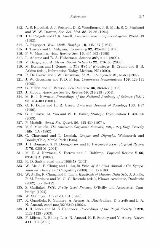
June 6, 2007 9:49 WSPC/Trim Size: 9in x 6in for Review Volume book
References 247
312. A. S. Klovdhal, J. J. Potterat, D. E. Woodhouse, J. B. Muth, S. Q. Muthandand W. W. Darrow, Soc. Sci. Med. 38, 79-88 (1994).
313. J. F. Padgett and C. K. Ansell, American Journal of Sociology 98, 1259-1319(1993).
314. A. Rapoport, Bull. Math. Biophys. 19, 145-157 (1957).315. J. Travers and S. Milgram, Sociometry 32, 425-443 (1969).316. P. V. Marsden, Ann. Review Soc. 16, 435-463 (1990).317. L. Adamic and B. A. Huberman, Science 287, 2115 (2000).318. V. Batgelj and A. Mrvar, Social Networks 22, 173-186 (2000).319. M. Bordens and I. Gomez, in The Web of Knowledge, B. Cronin and H. B.
Atkins (eds.), Information Today, Medson, NJ (2000).320. R. De Castro and J.W. Grossman, Math. Intelligencer 21, 51-63 (1999).321. J. W. Grossman and P. D. F. Ion, Congressus Numerantium 108, 129-131
(1995).322. G. Mellin and O. Persson, Scientometric 36, 363-377 (1996).323. J. Moody, American Society Review 69, 213-238 (2004).324. M. E. J. Newman, Proceedings of the National Academy of Science (USA)
98, 404-409 (2001).325. G. F. Davis and H. R. Greve, American Journal of Sociology 103, 1-37
(1996).326. G. F. Davis, M. Yoo and W. E. Baker, Strategic Organization 1, 301-326
(2003).327. P. Mariolis, Social Sci. Quart. 56, 425-439 (1975).328. M. S. Mizruchi, The American Corporate Network, 1904-1974, Sage, Beverly
Hills, CA (1982).329. G. Chartrand and L. Lesniak, Graphs and Digraphs, Wadsworth and
Brooks/Cole, Menlo Park (1986).330. J. J. Ramasco, S. N. Dorogovtsev and R. Pastor-Satorras, Physical Review
E 70, 036106 (2004).331. M. E. J. Newman, S. Forrest and J. Balthrop, Physical Review E 66,
035101(R) (2002).332. R. D. Smith, cond-mat/0206378 (2002).333. W. Aiello, F. Chung and L. Lu, in Proc. of the 32nd Annual ACm Sympo-
sium on Theory and Computing (2000), pp. 171-180.334. W. Aiello, F. Chung and L. Lu, in Handbook of Massive Data Sets, J. Abello,
P. M. Pardalos and M. G. C. Resende (eds.), Kluwer Academic, Dordrecht(2002), pp. 97-122.
335. S. Garfinkel, PGP: Pretty Good Privacy, O’Reilly and Associates, Cam-bridge (1994).
336. W. Stallings, BYTE 20, 161 (1995).337. X. Guardiola, R. Guimera, A. Arenas, A. Diaz-Guilera, D. Streib and L. A.
N. Amaral, cond-mat/0206240 (2002).338. J. H. Jones and M. S. Handcock, Proceedings of the Royal Society B 270,
1123-1128 (2003).339. F. Liljeros, R. Edling, L. A. N. Amaral, H. E. Stanley and Y. Aberg, Nature
411, 907 (2001).
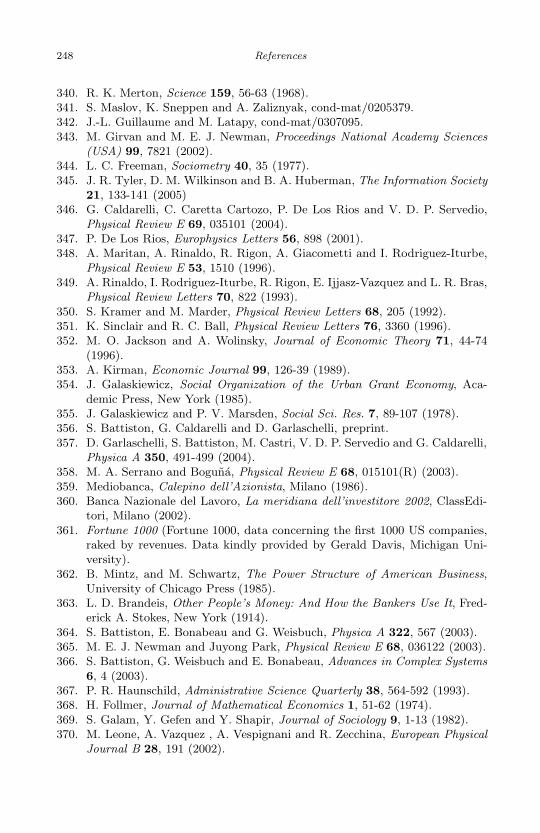
June 6, 2007 9:49 WSPC/Trim Size: 9in x 6in for Review Volume book
248 References
340. R. K. Merton, Science 159, 56-63 (1968).341. S. Maslov, K. Sneppen and A. Zaliznyak, cond-mat/0205379.342. J.-L. Guillaume and M. Latapy, cond-mat/0307095.343. M. Girvan and M. E. J. Newman, Proceedings National Academy Sciences
(USA) 99, 7821 (2002).344. L. C. Freeman, Sociometry 40, 35 (1977).345. J. R. Tyler, D. M. Wilkinson and B. A. Huberman, The Information Society
21, 133-141 (2005)346. G. Caldarelli, C. Caretta Cartozo, P. De Los Rios and V. D. P. Servedio,
Physical Review E 69, 035101 (2004).347. P. De Los Rios, Europhysics Letters 56, 898 (2001).348. A. Maritan, A. Rinaldo, R. Rigon, A. Giacometti and I. Rodriguez-Iturbe,
Physical Review E 53, 1510 (1996).349. A. Rinaldo, I. Rodriguez-Iturbe, R. Rigon, E. Ijjasz-Vazquez and L. R. Bras,
Physical Review Letters 70, 822 (1993).350. S. Kramer and M. Marder, Physical Review Letters 68, 205 (1992).351. K. Sinclair and R. C. Ball, Physical Review Letters 76, 3360 (1996).352. M. O. Jackson and A. Wolinsky, Journal of Economic Theory 71, 44-74
(1996).353. A. Kirman, Economic Journal 99, 126-39 (1989).354. J. Galaskiewicz, Social Organization of the Urban Grant Economy, Aca-
demic Press, New York (1985).355. J. Galaskiewicz and P. V. Marsden, Social Sci. Res. 7, 89-107 (1978).356. S. Battiston, G. Caldarelli and D. Garlaschelli, preprint.357. D. Garlaschelli, S. Battiston, M. Castri, V. D. P. Servedio and G. Caldarelli,
Physica A 350, 491-499 (2004).358. M. A. Serrano and Boguna, Physical Review E 68, 015101(R) (2003).359. Mediobanca, Calepino dell’Azionista, Milano (1986).360. Banca Nazionale del Lavoro, La meridiana dell’investitore 2002, ClassEdi-
tori, Milano (2002).361. Fortune 1000 (Fortune 1000, data concerning the first 1000 US companies,
raked by revenues. Data kindly provided by Gerald Davis, Michigan Uni-versity).
362. B. Mintz, and M. Schwartz, The Power Structure of American Business,University of Chicago Press (1985).
363. L. D. Brandeis, Other People’s Money: And How the Bankers Use It, Fred-erick A. Stokes, New York (1914).
364. S. Battiston, E. Bonabeau and G. Weisbuch, Physica A 322, 567 (2003).365. M. E. J. Newman and Juyong Park, Physical Review E 68, 036122 (2003).366. S. Battiston, G. Weisbuch and E. Bonabeau, Advances in Complex Systems
6, 4 (2003).367. P. R. Haunschild, Administrative Science Quarterly 38, 564-592 (1993).368. H. Follmer, Journal of Mathematical Economics 1, 51-62 (1974).369. S. Galam, Y. Gefen and Y. Shapir, Journal of Sociology 9, 1-13 (1982).370. M. Leone, A. Vazquez , A. Vespignani and R. Zecchina, European Physical
Journal B 28, 191 (2002).

June 6, 2007 9:49 WSPC/Trim Size: 9in x 6in for Review Volume book
Index
affinity, 71
airport network, 74
clustering, 75disparity, 76
strength distribution, 74
analytic layouts, 124
assortative generator, 57average nearest neighbors degree, 40
betweenness, 98
current-flow, 98
biological network, 83bipartite core, 136
board of directors, 219
assortativity, 225degree distribution, 224
statistical properties, 222
breadth first search, 136
centrality, 97
centrality layouts, 125circuit, 10
clique, 9, 95
clustered layouts, 126clustering
coefficient, 12
random walks, 108
connected component, 136strongly, 136
weakly, 136
connectivity, 10correlations
detailed balance, 37
three vertices, 45
two vertices, 41
coupling of traffic and topology, 91
cycle, 10
degree, 8, 135
distribution, 12
heterogeneity, 14
in-, 8, 135
out-, 8, 135
sequence, 8
weighted, 8
disassortative correlations, 55
edge, 5
multiple, 7
end vertices, 6
Erdos-Renyi model, 168
finite size effects, 170
food web, 195
spanning tree, 191
forest, 10
Gaussian distribution, 13
Girvan and Newman algorithm, 98
graph, 5
bipartite, 9
complete, 6
directed, 7
empty, 6
order, 6
oriented, 7
r-partite, 9
size, 6
weighted, 7
249

June 6, 2007 9:49 WSPC/Trim Size: 9in x 6in for Review Volume book
250 Index
Internetautonomous systems, 52average nearest neighbors degree,
175correlations, 173degree distribution, 168maps, 164small-world, 166
joint degree distribution, 38
L-shells, 101link clustering, 100links efficiency, 190local heterogeneity, 72, 88loop, 7
modelBarabasi-Albert, 25
degree distribution, 27degree exponents, 27rate equation, 25
clustered networks, 59configuration, 55copying, 144duplication divergence
rate equation, 29duplication-divergence, 27fitness, 21, 62
degree distribution, 22fitness and preferential attachment,
64growing, 56growing weighted networks, 30
degree distribution, 31hidden color, 61multi-layer, 145preferential attachment, 23Q-potts, 110random graphs, 18, 168
degree distribution, 19small-world, 32
shortcuts, 32weighted network, 84world wide web, 142
modularity, 96
maximization, 102multigraph, 7
networkassortative, 41collaboration, 207communication, 207disassortative, 41Markovian, 39mutual recognition, 208protein interaction, 47resistors, 99
approximate, 106scale-free, 14scientific collaboration, 50social, 206
assortativity, 210clustering, 213
world airport, 53network efficiency, 99networks
evolving, 18static, 18
optimisationconstrained, 106extremal, 103greedy, 102
PageRank, 140path, 9, 136
Eulerian, 10Hamiltonian, 10
Poisson’s distribution, 13preferential attachment and
duplication, 29preprint archive, 17
random graph, 18rich-club phenomenon, 76
scientific collaboration network, 80clustering, 82degree distribution, 80disparity, 82topology weight correlation, 80

June 6, 2007 9:49 WSPC/Trim Size: 9in x 6in for Review Volume book
Index 251
six degrees of separation, 11small world, 11spectral analysis, 104strength, 69subgraph, 8
induced, 136
taxonomy, 192tier, 174traversal, 136tree, 10
leaves, 11root, 11
treesspanning, 188
trophic interactions, 186
urban network, 77clustering, 78degree distribution, 77disparity, 78
strength, 78
vertex, 5adjacent, 6incident, 6
visualizationspectral layout, 121spring embedder methods, 117
walk, 136web of trust, 51weight, 68
clustering coefficient, 69distribution, 68
world trade web, 53world wide web
cliques, 142crawl, 137degree distributions, 138WebBase, 138