intensity-field correlations of non ... - umd physics

INTENSITY-FIELD CORRELATIONS OF NON-CLASSICALLIGHT

H. J. CARMICHAELDepartment of PhysicsUniversity of AucklandPrivate Bag 92019Auckland, 1301, New Zealand.G. T. FOSTERDepartment of Physics and AstonomyHunter College, CUNYNew York, NY 10021, United StatesL. A. OROZCO, J. E. REINERDepartment of Physics and AstronomyState University of New YorkStony Brook NY 11794-3800, United States

AND

P. R. RICEDepartment of PhysicsMiami UniversityOxford, OH 45056, United States

Abstract. The intensity-field correlation function of the electromagneticfield is a tool for studying the quantum fluctuations of light. This review in-troduces the correlation function and its relationship to quadrature squeez-ing, develops conditions ( Schwartz inequalities) to distinguish betweennonclassical and classical field fluctuations, and discusses its connection toweak measurements. The theoretical ideas are illustrated by calculationsfor three sample systems: the optical parametric oscillator, a cavity QEDsystem, and the composite system of a single atom coupled to an opticalparametric oscillator. The results of experimental measurements on a cavityQED system are also reviewed.

2 H. J. CARMICHAEL ET AL.

Table of Contents

1 INTENSITY-FIELD CORRELATIONS OF NON-CLASSICALLIGHT 11 Introduction . . . . . . . . . . . . . . . . . . . . . . . . . . . 42 Theory . . . . . . . . . . . . . . . . . . . . . . . . . . . . . . 6

2.1 The Intensity-Field Correlation Function hθ(τ) . . . 62.2 Classical Bounds for hθ(τ) . . . . . . . . . . . . . . . 102.3 Time Reversal Properties of hθ(τ) . . . . . . . . . . 112.4 Intensity-Field Correlations in Classical Optics . . . 12

3 Examples . . . . . . . . . . . . . . . . . . . . . . . . . . . . 133.1 Optical Parametric Oscillator . . . . . . . . . . . . . 163.2 Cavity QED . . . . . . . . . . . . . . . . . . . . . . 183.3 Two-Level Atom in an Optical Parametric Oscillator 28

4 Experiment in Cavity QED . . . . . . . . . . . . . . . . . . 324.1 Cavity QED Apparatus . . . . . . . . . . . . . . . . 334.2 Conditional Homodyne Detector . . . . . . . . . . . 344.3 Measurements . . . . . . . . . . . . . . . . . . . . . 36

5 Equal-Time Cross- and Auto-Correlations . . . . . . . . . . 415.1 Cross-Correlations . . . . . . . . . . . . . . . . . . . 42

6 Quantum Measurements and Quantum Feedback . . . . . . 456.1 Weak Measurements . . . . . . . . . . . . . . . . . . 456.2 Vacuum State Squeezing Versus Squeezed Classical

Noise . . . . . . . . . . . . . . . . . . . . . . . . . . 466.3 Application of hθ(τ) to Quantum Feedback . . . . . 47

7 Conclusion and Outlook . . . . . . . . . . . . . . . . . . . . 50

3


1. Introduction

Studies of the fluctuations of light have occupied quantum optics since itsbeginnings. Experimental work in the field has followed two broad lines,the first focused on intensity fluctuations and the measurement of correla-tions between pairs of photon detections [particle aspect of light] (Brownand Twiss (1956), Kimble, Dagenais and Mandel (1977)), and thesecond primarily concerned with squeezing experiments where the fluctu-ation variance of a quadrature amplitude of the optical field is measured[wave aspect of light] (Slusher, Hollberg, Mertz, Yurke and Valley(1985), Loudon and Knight (1987), Kimble and Walls (1987)).

Until recently, these two lines of investigation remained separate. It isnow possible, however, to combine them in a new approach that detects thefluctuations of an electromagnetic field by correlating its intensity and am-plitude (Carmichael, Castro-Beltran, Foster and Orozco (2000),Foster, Orozco, Castro-Beltran and Carmichael (2000a)). Theapproach draws the particle and wave aspects of light together, and opensup a third-order correlation function of the electromagnetic field to ex-perimental study. The new measurement strategy builds upon the rela-tionship between quantum optical correlation functions and conditionalmeasurements (Mandel and Wolf (1995)), and its physical interpre-tation is therefore illuminated through quantum trajectory calculations(Carmichael (1993a)).

Historically, it was the development of the intensity-intensity correla-tion technique of Hanbury Brown and Twiss (HBT) (Brown and Twiss(1956)) that provided the stimulus for a systematic treatment of optical co-herence within the framework of quantum mechanics (Glauber (1963a),Glauber (1963b), Glauber (1963c)). A notable feature of the HBT ap-proach is its reliance on a conditional measurement—i.e., data is collectedon the cue of a conditioning photon count that identifies those times whenan intensity fluctuation is in progress. In this way, the average fluctuationis recovered as a conditional evolution over time, and a sensitive probe ofthe nonclassicality of light is obtained.

The standard squeezing measurement is not, by way of contrast, a con-ditional measurement. Through balanced homodyne detection (Yuen andChan (1983a), Yuen and Chan (1983b)), it effectively measures the sub-Poissonian variance of a photon counting distribution, after the photoncounts have been integrated over many correlation times. The measure-ment is insensitive to fluctuations at low photon flux and the observeddegree of squeezing is degraded by collection and detection inefficiencies.The measurement is resolved in the frequency domain and does not recoveran evolution of the fluctuations over time.

INTENSITY-FIELD CORRELATIONS 5

The intensity-field correlation function is measured through the con-ditional detection of the quadrature amplitude fluctuations of light. Themeasurement cross-correlates the photocurrent of a balanced homodynedetector (BHD) with an initiating photon count in a natural extensionof the HBT technique. It is extremely sensitive to the nonclassicality oflight at low photon flux (weakly squeezed light) and, given sufficient detec-tion bandwidth, resolves the fluctuations in time. For the case of Gaussianstatistics, Carmichael, Castro-Beltran, Foster and Orozco (2000)showed that the full spectrum of squeezing is recovered from the Fouriertransform of the time-resolved fluctuation. The measurement, like the HBTtechnique, is independent of detection efficiency, except for the inevitableefficiency-dependence in the signal-to-noise ratio.

To date, intensity-field correlations have been explored for the opti-cal parametric oscillator (OPO) (Carmichael, Castro-Beltran, Fos-ter and Orozco (2000)), in both theoretical (Carmichael, Castro-Beltran, Foster and Orozco (2000), Reiner, Smith, Orozco, Carmichaeland Rice (2001)) and experimental (Foster, Orozco, Castro-Beltranand Carmichael (2000a), Foster, Smith, Reiner and Orozco (2002))studies of cavity QED, and for a single two-level atom coupled to an OPO(Strimbu and Rice (2003)). On the theoretical side, connections havebeen made to fundamental questions in quantum measurement theory andstatistical physics. Wiseman (2002), for example, has demonstrated a con-nection with weak measurements. Carmichael (2003) has shown that, incontrast to a conventional squeezing measurement, conditional homodynedetection distinguishes qualitatively between vacuum state squeezing andsqueezed classical noise. Denisov, Castro-Beltran and Carmichael(2002) explored the time-reversal properties of the intensity-field correla-tions. They show that while the intensity-intensity correlation function isnecessarily time symmetric, the intensity-field correlation function may betime asymmetric for non-Gaussian fluctuations. The time asymmetry indi-cates a breakdown of detailed balance.

In related but earlier work, Yurke and Stoler (1987) proposed us-ing intensity-field correlations between signal and idler channels to prepareand observe Fock sates in the process of parametric down conversion. Re-cently, the tomographic reconstruction of a one-photon state was achievedworking with an extension of their technique (Crispino, Giuseppe, Mar-tini, Mataloni and Kanatoulis (2000), Lvovsky, Hansen, Aichele,Benson, Mlynek and Schiller (2001)). The reconstruction relies on atime-integrated correlation, since the time scales in parametric down con-version are too short for current technology to follow the fluctuation overtime. Intensity-field correlations also arise, more indirectly, in various othercontexts: Vyas and Singh (2000), Deng, Erenso, Vyas and Singh


(2001) on the degenerate OPO and Vogel (1991) for resonance fluores-cence.

The review is organized as follows. We begin, in Sec. 2, by presentingthe general theoretical framework for the measurement of intensity-fieldcorrelations, including a discussion of the time-reversal properties of thecorrelation function. Section 3 illustrates the ideas with theoretical calcula-tions for three specific quantum optical systems. The results of experimentsin cavity QED are then presented in Sec. 4; there we give a thorough de-scription of the experimental apparatus required. In Sec. 5 we review workon time-integrated intensity-field correlations in parametric down conver-sion. We finish, in Sec. 6, with an overview of the impact intensity-fieldcorrelations have made in the area of quantum measurement theory.

2. Theory

Figure 1 shows a schematic of the intensity-field correlator. It is based uponthe HBT intensity correlator implemented in the modern “start”/“stop”scheme found for example in Foster, Mielke and Orozco (2000b). Theprincipal difference is that there is a balanced homodyne detector (BHD) inplace of the second photon detector in what would normally be the “stop”channel; so it is appropriate to name this method as conditional homodynedetection (CHD). Operation of the correlator proceeds as follows: within afew correlation times before and after each “start”, the homodyne currentI(t) is digitized, recorded, and used to update a cumulative average; aver-aging Ns such samples reduces the shot noise so that the surviving signal isa conditional average of the quadrature amplitude fluctuations of the inputoptical field.

2.1. THE INTENSITY-FIELD CORRELATION FUNCTION Hθ(τ)

For a more detailed analysis of the measurement, we consider a generaloptical source with power bandwidth 2κ and output source-field

√2κb (in

units of the square-root of photon flux). In order to record a nonzero signal,the firing of the “start” detector must be biased towards the identificationof quadrature amplitude fluctuations of a particular sign. To achieve this,a coherent offset of the source-field is generally needed (BS1 in Fig. 1).The offset also carries an adjustable phase, allowing the free selection ofthe quadrature to be measured. The input field to the correlator is thenexpressed in terms of the source field as

√2κa =

√2κ(b + Aeiϑ), (1)

where Aeiϑ is determined by the complex amplitude of the offset. [A similaroffset is used in some quantum state reconstruction schemes (Banaszek


LO

I(t)

(1-η)1/2 a^^a^b

Source

offset

BS2BS1

tj

η1/2 a^

Figure 1. Schematic of the intensity-field correlator. The homodyne current I(t) issampled over a series of time windows, tj − τmax ≤ t ≤ tj + τmax, each centered on a“start” time tj .

and Wodkiewicz (1996), Wallentowitz and Vogel (1996), Lutter-back and Davidovich (1997)).] Sometimes the source-field has a non-zeromean amplitude, as is the case for the cavity QED system considered inSec. 4. In such a case, the offset is not needed.

A fraction η of the input light is now sent to the balanced homodynedetector, with the remaining fraction 1 − η going to the photon detectorin the “start” channel (BS2 in Fig. 1). The photon flux operator at thephoton detector is thus given in terms of the photon number operator forthe source field (for simplicity, free-field operators are neglected as they donot contribute to normal-ordered averages):

S = (1− η)2κa†a. (2)

The balanced homodyne detector samples the quadrature phase amplitudethat is in phase with the local oscillator field (LO in Fig. 1), with operatorvalue

D = 2√

η2κaθ, aθ ≡ 12 [ae−iθ + a†eiθ], (3)

where θ is the LO phase. The conditional homodyne photocurrent, averagedover the Ns “starts”, is then

Hθ(τ) =〈 : S(t)D(t + τ) : 〉

〈S〉 + ξ(τ); (4)


〈 : : 〉 denotes time and normal ordering, and ξ(t) is the residual local oscil-lator shot noise that is present because the ensemble average is taken overa finite number of samples only; its magnitude depends in the usual wayon detection bandwidth and the number of samples Ns.

For positive τ , Hθ(τ) can be factorized in a straightforward way withthe help of the quantum regression formula to give

Hθ(τ) = 〈D(τ, θ)〉c + ξ(τ), (5)

where the subscript c denotes conditioning of the state at time t on the de-tection of a photon. This is one of the most powerful results of the intensity-field correlation function in its quantum mechanical formulation; it givesaccess to the conditional dynamics of the quadrature phase amplitudes ofthe field, similar to the manner in which the intensity-intensity correlationfunction gives the conditional dynamics of the intensity (Carmichael,Brecha and Rice (1991), Brecha, Rice and Xiao (1999)). For neg-ative τ , a construction of the post-selected conditional dynamics may bemade on the basis of Baysean inference (Sec. 6.1).

When the source field is small and non-classical, its fluctuations, amanifestation of the uncertainty principle, dominate over its steady-stateamplitude. It is these fluctuations that are of interest, and therefore theinput-field operator a is conveniently decomposed as a = α + ∆a, withα = 〈a〉 = |α|eiφ, and ∆a = ∆b ≡ b − 〈b〉 the fluctuation of interest.We now substitute Eqs. (2) and (3) into Eq. (4), and at the same timemake the decomposition into a mean field plus fluctuation. In addition,for the present discussion we make the assumption, clearly valid for thecase of Gaussian statistics, that third order moments of the field fluctua-tions vanish. The resulting correlation function in terms of the quadraturefluctuation ∆aφ = (∆ae−iφ + ∆a†e+iφ)/2 is:

Hθ,φ(τ) =√

η2κ2|α|(

cos(φ− θ) +2〈 :∆aφ(0)∆aθ(τ) : 〉|α|2 + 〈∆a†∆a〉

)

+ξ(τ). (6)

The assumption of Gaussian statistics is not necessary, and as Denisov,Castro-Beltran and Carmichael (2002) have shown, presumes de-tailed balance, which for some systems does not hold (see Sec. 2.3). It isonly for this special case, though, that there is a direct and simple connec-tion with the spectrum of squeezing.

The maximum signal to noise ratio is obtained with the coherent inten-sity much larger than the incoherent intensity, |α|2 À 〈∆a†∆a〉 = 〈∆b†∆b〉.If, however, we choose the coherent offset in such a way that the coherentand incoherent intensities are the same,

|α|2 = 〈∆a†∆a〉 = 〈∆b†∆b〉, (7)


although one gives up a little in signal-to-noise ratio (a factor of√

2), onegains a different perspective in the discussion of nonclassical features in thecorrelation function. With the choice of maximal signal-to-noise ratio, andthe mean field adjusted to be in phase with the local oscillator (φ = θ), weobtain a normalized correlation function after dividing Eq. (6) by

√η2κ2|α|

Carmichael, Castro-Beltran, Foster and Orozco (2000),

hθ(τ) = 1 +2

1 + |α|2/〈∆a†∆a〉〈 :∆aθ(0)∆aθ(τ) : 〉

〈∆a†∆a〉 +ξ(τ)√

η2κ2|α| . (8)

In the limit of negligible residual shot noise (Ns → ∞), we denote thecorrelation function by

hθ(τ) = 1 +2

1 + |α|2/〈∆a†∆a〉〈 :∆aθ(0)∆aθ(τ) : 〉

〈∆a†∆a〉 . (9)

The spectrum of squeezing (Collett and Gardiner (1984), Carmichael(1987)) may then be written as

S(Ω, θ) = 4F

∫ ∞

0dτ cos(2πΩτ)[hθ(τ)− 1], (10)

where F = 2κ〈a†a〉 = 2κ(|α|2 + 〈∆a†∆a〉) is the input field photon flux.Thus, hθ(τ) achieves a time-resolved measurement of the quadrature am-plitude fluctuations of the squeezed electromagnetic field. Notice that themeasurement is independent of detection and collection efficiencies, thoughthe efficiency η does appear in Eq. (8) as one of the factors affecting thesingle-to-noise ratio. The measured degree of squeezing also depends onthe determination of the photon flux F . The technique is nevertheless lesssensitive to efficiencies than traditional squeezing measurements (Bachor(1998)) since the propagation losses are taken into account by the normal-ization of hθ(τ).

Under the assumed conditions of Gaussian statistics, hθ(τ) is necessarilysymmetric in time. We may then write the Fourier pair:

S(Ω, θ) = 2F∫ ∞

−∞dτ exp(i2πΩτ)[hθ(τ)− 1],

hθ(τ)− 1 =1

4πF

∫ ∞

−∞dΩexp(−i2πΩτ)S(Ω, θ). (11)

Notice that the photon flux plays a role, in inverse relationship, in therelative sizes of the spectrum of squeezing and the intensity-field correlationfunction. From this, it would seem that for large photon flux, nonclassicaleffects might be observed more readily in measurements of the spectrum


of squeezing, and for low photon flux, in measurements of hθ(τ). Thereis also a relationship between the time averaged hθ(τ) and the degree ofsqueezing at zero frequency, and between the frequency averaged spectrumof squeezing and hθ(0):

S(0, θ) = 2F∫ ∞

−∞dτ [hθ(τ)− 1],

hθ(0)− 1 =1

4πF

∫ ∞

−∞dΩS(Ω, θ). (12)

2.2. CLASSICAL BOUNDS FOR Hθ(τ)

Squeezing is directly related to a reduction in the variance of fluctuationsin one of the field quadrature amplitudes. The squeezing manifests itself inthe time domain through violations of classical bounds on the correlationfunction hθ(τ). Carmichael, Castro-Beltran, Foster and Orozco(2000) derived two such classical bounds whose derivation we review here.

We begin from the observation that the fluctuation intensity may bewritten as a sum of the normal-ordered variances for the quadrature fieldamplitudes:

〈∆a†∆a〉 = 〈 :∆a2θ : 〉+ 〈 :∆a2

θ+π/2 : 〉. (13)

Combining Eq. (9) with this result leads to an expression for hθ(0) in theform

hθ(0)− 1 =2

1 + |α|2/〈∆a†∆a〉〈 :∆a2

θ : 〉〈 :∆a2

θ : 〉+ 〈 :∆a2θ+π/2 : 〉 . (14)

In the classical case, both quadrature variances are greater than zero, sowe may deduce both lower and upper bounds for hθ(0):

0 ≤ hθ(0)− 1 ≤ 21 + |α2|/〈∆a†∆a〉 . (15)

The upper bound, in particular, is quite different from the familiar boundson the intensity-intensity correlation function. Generalizing to non-zerotime delay, we have the Schwarz inequality

|〈 :∆aθ(0)∆aθ(τ) : 〉|2 ≤ 〈 :∆a2θ(0) : 〉〈 :∆a2

θ(τ) : 〉 = 〈 :∆a2θ : 〉2, (16)

which implies

|hθ(τ)− 1| ≤ 21 + |α|2/〈∆a†∆a〉

|〈 :∆a2θ : 〉|

〈∆a†∆a〉 , (17)


or|hθ(τ)− 1| ≤ |hθ(0)− 1|. (18)

This second condition and the lower bound in Eq. (15) are similar tothe classical bounds associated with the definition of photon antibunch-ing (Kimble, Dagenais and Mandel (1977), Walls (1979), Loudon(1980), Paul (1982)).

For a classical field such that the intensity is much larger than thevariance, one can prove in addition an inequality relating the intensity-fieldcorrelation function hθ(0) and the intensity-intensity correlation functiong(2)(0); one finds

|hθ(0)| ≤√

g(2)(0), (19)

If there is an offset field α such that the intensity is equal to the variance,then the inequality is:

|hθ(0)| ≤√

2g(2)(0). (20)

2.3. TIME REVERSAL PROPERTIES OF Hθ(τ)

The time symmetry of the cross-correlation of fluctuations about thermalequilibrium, 〈B(t+τ)A(t)〉 = 〈B(t−τ)A(t)〉, where A and B are thermody-namic quantities, has a central place in statistical physics; it provides thefundamental basis for the Onsager relations (Onsager (1931), Casimir(1945)). The symmetry follows from microscopic reversibility (A and B areassumed both symmetric or antisymmetric under time reversal), which re-quires that the equilibrium state be maintained through detailed balance(Tolman (1938)). In quantum optics, one is usually concerned with steadystates away from equilibrium, where correlation functions of the light emit-ted by an open system are measured through photoelectric detection. Thedetected radiation field is outgoing and absorbed by the environment; itssteady state is thus manifestly not symmetric under time reversal. In a sit-uation like this, fluctuations about the steady state may exhibit a specifictime order.

The majority of studies in quantum optics have focused, nonetheless,on time-symmetric correlations. There are two main reasons for this. First,nonclassical phenomena such as photon antibunching and squeezing dealwith autocorrelations, 〈A(t + τ)A(t)〉, which are symmetric by definitionfor a stationary process. Second, although detailed balance is not requiredby microreversibility away from equilibrium (Klein (1955), Tomita andTomita (1973), Tomita and Tomita (1974)), it may follow, nevertheless,from symmetry and boundary conditions (Graham (1971)). A laser, forexample, maintains its steady state through detailed balance (Graham


and Haken (1971)) in spite of the fact that it operates far from thermalequilibrium.

The cross-correlation of field intensity and amplitude provides, in prin-ciple, for the observation of time asymmetric correlations. Concerning therequisite failure of detailed balance, Tomita and Tomita (1973) andTomita and Tomita (1974) determined what is needed in the case ofGaussian fluctuations: there must exist “a coupling between more than onedegrees of freedom, so that there can be a direction” in the nonequilib-rium flux through the system. Such a coupling—between the atom(s) andthe cavity field—is a central feature in cavity QED. In the case of Gaus-sian fluctuations, however, hθ(τ) reduces to the autocorrelation of Eq. (8),which is necessarily time symmetric. It follows that conditional detectionof the kind considered can reveal time asymmetry only in a regime wherethe fluctuations are non-Gaussian (cross-correlating a “start” detection inone channel with homodyne detection in another provides wider possibili-ties). In this case a time asymmetric hθ(τ) not only indicates a breakdownof detailed balance, it also provides direct evidence of non-Gaussian fluctu-ations.

We might expect resonance fluorescence to provide the simplest ex-ample of a time asymmetric hθ(τ); its fluctuations are non-Gaussian and acoupling between degrees of freedom enters through the optical Bloch equa-tions. Quantum transitions, on the other hand, occur between two statesonly; this suggests that detailed balance has to hold, since it is the only sortof balance that can maintain a steady state (Klein (1955)). It is indeedreadily shown that hθ(τ) is symmetric in resonance fluorescence.

The two-state restriction is lifted, on the other hand, for multiphotonscattering in cavity QED. In this context, Denisov, Castro-Beltranand Carmichael (2002) recently computed time-asymmetric intensity-field correlation functions which demonstrate the breakdown of detailedbalance. Examples of their results are presented in Sec. 3.2.3.

2.4. INTENSITY-FIELD CORRELATIONS IN CLASSICAL OPTICS

In Chapter 8 of their celebrated book, Mandel and Wolf (1995) treatcorrelation functions of arbitrary order in the field, both even and odd or-ders. They develop Schwarz inequalities for cross-correlations of arbitraryorder and show that in the case of Gaussian noise, the odd-order correla-tion functions are zero, the result we drew on in passing from Eq. (4) to(6). Moreover, when the field is quasi-monochromatic and the statisticalensemble characterizing the fluctuations is stationary—though not neces-sarily Gaussian—the odd-order correlations are zero except at very highorders.


The same authors treat quantum mechanical correlation functions ofarbitrary order in Chapter 12 of their book, where they note that theodd-order correlation functions arise naturally in connection with nonlin-ear media. In these media the quantum expectation value of the intensitydepends on odd-order correlation functions (involving unequal numbers ofcreation and annihilation operators). They show again, however, that whenthe electromagnetic field is stationary and quasimonochromatic, the odd-order correlations must vanish unless the order is very large.

The approach presented in 1 for the intensity-field correlation strictlyspeaking uses four fields: two for the intensity detection and two for thehomodyne detection, except that the contributions of the strong local os-cillator are averaged away.

3. Examples

The intensity-field correlation function has been calculated for three im-portant sources of nonclassical light. We review the results in this section.The first is the Optical Parametric Oscillator (OPO) well below threshold(Carmichael, Castro-Beltran, Foster and Orozco (2000)), whereresults for hθ(τ) clarify how such a source of highly bunched light can nev-ertheless show quadrature squeezing. For the second, a cavity QED source,the intensity-field correlation captures the oscillatory exchange of excitationbetween the cavity mode and atoms, the normal-mode or polariton oscilla-tion; the oscillation is related to the spectrum of squeezing (Carmichael,Castro-Beltran, Foster and Orozco (2000)) and a discussion ofits degradation through spontaneous emission is given (Reiner, Smith,Orozco, Carmichael and Rice (2001)). The third example is a two-level atom coupled to the intracavity field of an OPO, which shows a mix-ture of the behavior demonstrated in the first two examples (Strimbu andRice (2003)).

Various methods are available for calculating the intensity-field cor-relation function. Most directly, the two-time average in Eq. (4) may beevaluated from a knowledge of the source master equation,

dρ

dt= Lρ, (21)

using the quantum regression formula. Generally, a different formula appliesfor positive and negative τ (Carmichael (1999)), allowing for the timeasymmetry of Sec. 2.3. We have

〈 : S(t)D(t + τ) : 〉√η2κ〈S〉 = 〈a†a〉−1

tr[ae−iθeL|τ |(aρssa

†)] + c.c. τ ≥ 0

tr[(a†a)eL|τ |(ae−iθρss)] + c.c. τ ≤ 0,

(22)


where a is related through Eq. (1) to the source quasimode b.Alternatively, a simulation of the conditional averaging process that

yields the correlation function may be given within the framework of quan-tum trajectory theory. As is well known, the theory of quantum trajectoriesis formulated around the experimental data, viewed as a stochastic mea-surement record (Carmichael (1993a)). For the detection scheme of Fig. 1,the record comprises the continuous homodyne current, I(t), and the set ofstart times tj. The source quasimode is in a quantum state |ψREC(t)〉, con-ditioned on this record. Realizations of I(t),tj, and |ψREC(t)〉 obey a setof stochastic differential equations that may be simulated on a computer.By sampling an ongoing realization of I(t), one calculates the conditionallyaveraged photocurrent as

Hθ(τ) =1

Ns

Ns∑

j=1

I(tj + τ). (23)

To carry out this program, the explicit quantum stochastic process (un-ravelling of the density operator ρ) must be formulated in line with theprinciples introduced in Secs. 8.4 and 9.4 of Carmichael (1993a), gener-alized in this case to include the coherent offset of Fig. 1 and to combine thecontinuous evolution under homodyne detection with the quantum jumpconditioning, |ψREC(tj)〉 → a|ψREC(tj)〉, at the start times tj (the state|ψREC(t)〉 is not normalized). Clearly, in time step dt, the probability of astart count is (1 − η)2κ〈(a†a)(t)〉RECdt. Between starts, |ψREC(t)〉 evolvesaccording to the stochastic Schroedinger equation

d|ψREC(t)〉 = [(HS/ih− 2κAe−iφb)dt +√

ηκ ae−iθdQt]|ψREC(t)〉, (24)

where HS is the non-Hermitian source Hamiltonian. The source state isconditioned through this equation on the ongoing realization of charge,

dQt =√

η2κ 〈aθ〉RECdt + dWt, (25)

deposited in the homodyne detector output circuit; the Wiener incrementdWt incorporates the shot noise. The simple filtering equation 26 introducesa realistic detection bandwidth Γ:

dI = −Γ(Idt− dQt). (26)

If spontaneous emission is present, it may be incorporated in the usual waythrough additional quantum jumps.

The limit of weak excitation is a special case, since in this limit thecorrelation function is time symmetric and may be calculated from the


quantum trajectory equations by a straightforward analytical method. Wewrite

|ψREC(t)〉 =2∑

n+m=0

Cn,m(t)|n, m〉 (27)

where n denotes the photon number of the source quasimode, and m isthe set of all other relevant quantum numbers (referring to the internalstates of atoms in a cavity QED system, for example). Note that under theassumption of weak excitation, we may truncate the expansion at the levelof two quanta. This is the minimal nontrivial truncation; one quantum isrequired to provide the “start” count, and at least one other is needed ifthere is to be a nontrivial conditional signal at the BHD. Note now thatfor weak excitation, the “start”counts are extremely infrequent on the timescale taken by the source to relax to its steady state. The time intervalbetween one “start” and the next is then almost certain to be long enoughfor the steady state,

|ψssREC〉 =

2∑

n+m=0

Cssn,m|n, m〉, (28)

to be reached. The approach to the steady state may be calculated from

d|ψREC〉dt

=1ih

HS |ψREC〉, (29)

where the terms proportional to a and b in Eq. (24) are neglected as higherorder contributions. The conditional state after each “start” is now obtainedas

|ψREC(t+j )〉 ≡1∑

n+m=0

Cn,m(t+j )|n, m〉 =

a|ψssREC〉√

〈ψssREC|a†a|ψss

REC〉, (30)

and solving Eq. (29) with this state as the initial condition yields

|ψREC(tj + τ)〉 =2∑

n+m=0

Cn,m(tj + τ)|n, m〉. (31)

From Eqs. (1), (28), and (31), we obtain

〈aθ〉ss = Re[(

Css1,m=0 + Aeiϑ

)e−iθ

], (32)

〈aθ(tj + τ)〉REC = Re[

C1,m=0(tj + τ) + Aeiϑ]e−iθ

, (33)


χ(2)

b(2ω)

a(ω)^

^

γa

γb

ε(2ω)

Figure 2. Schematic of the OPO. A classical drive E , of frequency 2ω, injects energy intoa cavity which contains a medium that has a nonlinear susceptibility χ(2). The output isa field at the subharmonic frequency ω.

and finally, taking the limit Ns →∞ in Eq. (23) (also Γ →∞), the resultfor the normalized correlation function is

hθ(τ) ≡ Hθ(τ)√η2κ〈aθ〉ss =

Re[

C1,m=0(tj + τ) + Aeiϑ]e−iθ

Re[(

Css1,m=0 + Aeiϑ

)e−iθ

] . (34)

3.1. OPTICAL PARAMETRIC OSCILLATOR

Because of its simple nonlinearity, the process of parametric down con-version in a cavity has been the subject of extensive research in quantumoptics. This process is the basis of the optical parametric oscillator (OPO),which is modelled (see Fig. 2) by two modes of the electromagnetic field,with frequencies ωa and ωb, and a nonlinear interaction proportional toih(a†2b− a2b†). The Hamiltonian for the two coupled modes may be writ-ten as

H = hωaa†a + hωbb

†b +ihχ

2(a†2b− a2b†). (35)

Energy conservation requires that the frequencies are related, with ωb =2ω, ωa = ω. The coupling χ between the modes is proportional to thesecond order nonlinear susceptibility of the medium, χ(2). In addition to theinteraction shown, the modes also couple to reservoirs with decay constantsγa and γb to account for cavity loss, and there is a strong coherent drive Eof cavity mode b. The OPO shows a point of instability as a function of thedrive at E = Eth ≡ γaγb/χ; below this threshold the subharmonic mode haszero mean amplitude, while for E > Eth a nonzero mean field is establishedand parametric oscillation sets in.


The fluctuations in this system exhibit very large squeezing just be-low threshold (Collett and Gardiner (1984), Collett and Gar-diner (1985)). Conditions of low photon flux, well below threshold wherethe squeezing is small, are of particular interest from the point of view ofthe intensity-field correlations. Although the squeezing is small, the outputspectrum is a Lorentzian squared (Collett and Loudon (1987)), a mani-festation of squeezing induced linewidth narrowing (Rice and Carmichael(1988)). The output intensity shows very large bunching as the photons arecreated in pairs, a condition that has been of interest for producing a con-ditional source of single photons for quantum cryptography.

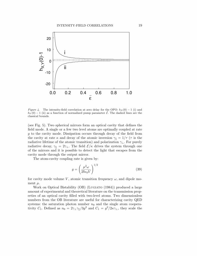
With regard to the intensity-field correlation, conditions of low photonflux are of particular interest because they lead to extremely large violationsof the upper bound of Eq. (15) (Carmichael, Castro-Beltran, Fosterand Orozco (2000)). The OPO with normalized pump parameter E ¿ 1,(E ≡ E/Eth) has quadrature variances and fluctuation intensity (Milburnand Walls (1981))

〈 : (∆qX)2 : 〉 ≈ E(1 + E)/4, (36)〈 : (∆qY )2 : 〉 ≈ −E(1− E)/4, (37)

and〈∆a†∆a〉 = 〈 : (∆qX)2 : 〉+ 〈 : (∆qY )2 : 〉 ≈ E2/2. (38)

The ratio 〈 : (∆qX,Y )2 : 〉/〈∆a†∆a〉 which enters on the right-hand side ofEq. (14) is of the order of 1/E . If E ¿ 1, the upper bound in Eq. (15) maybe exceeded by orders of magnitude.

Figures 3i and ii illustrate this prediction for broadband detection. Wellbelow threshold, where the squeezing is small (8% at line center), the classi-cal bounds are violated dramatically. A violation exists for both quadraturesof the field. It is permitted because of the anomalous phase of the fluctu-ation in Fig. 3ii, where, although the BHD current sampling is triggeredby photon counts, the averaged data records a fluctuation that is out ofphase with the offset; surely trigger counts would be more probable at thetimes of in phase fluctuations. The anomalous phase allows the sum of thequadrature variances to be much smaller than the modulus of either takenindividually, and hence leads to the large violation of inequality (15).

The results displayed in Fig. 3 show that conditional homodyne detec-tion is not simply an alternate method for the detection of squeezed light,but provides a completely different window on its nonclassicality. This isunderlined by Fig. 4, where the violation of inequality (15) is increasing fordecreasing pump parameter, while the squeezing and photon flux both de-crease. For small E , CHD detects anomalously large fluctuations of the fieldamplitude which are isolated in time through the conditional measurement.


-14 -7 0 7 14-6

0

6

12

18

24

30i

κτ-14 -7 0 7 14

-24

-18

-12

-6

0

6 ii

h y(τ

)κτ

h x(τ

)

Figure 3. Quantum trajectory simulation of CHD for the OPO: (i) X-quadrature am-plitude (unsqueezed), (ii) Y -quadrature amplitude (squeezed); with intracavity photon

number 〈a†a〉 = 2.0 × 10−4 (E = 0.02), η = 0.5, Ns = 10, 000. The dashed lines are theclassical bounds.

It records only the real fluctuations associated with the rare two-photonpulses seen in direct photon detection. While the intensity-intensity cor-relation of the photon pulses is highly bunched and looks classical, withg(2)(0) ∼ 1/E2, CHD resolves this correlation into quadrature amplitudecomponents and uncovers the anomalous phase behavior at the level of thefield amplitude.

In related work, several authors have used the beating of a local oscilla-tor with a signal field on a beam splitter to enhance the ability to measurenonclassical effects such as photon antibunching and squeezing. This in-cludes work by Vogel (1991) on resonance fluorescence, and Vyas andSingh (2000) and Deng, Erenso, Vyas and Singh (2001), and on theOPO. In the latter case, the output of the OPO mixed with the LO yieldsantibunched light, whereas it is highly bunched on its own. Neither of theseschemes relies on a conditioned measurement. A scheme that does use aconditioned measurement to see antibunching in an OPO system has re-cently been proposed by Leach, Strimbu and Rice (2003). Siddiqui,Erenso, Vyas and Singh (2003) discuss conditional measurements asprobes of quantum dynamics and show that they provide different ways tocharacterize quantum fluctuations in a subthreshold degenerate OPO.

3.2. CAVITY QED

We next consider a cavity QED system that consists of a single mode ofthe electromagnetic field interacting with a collection of two-level atoms


0.0 0.2 0.4 0.6 0.8 1.0

-20

-10

0

10

20

ii

i

h X,Y

(0)-

1

ε

Figure 4. The intensity-field correlation at zero delay for the OPO: hX(0) − 1 (i) andhY (0) − 1 (ii) as a function of normalized pump parameter E . The dashed lines are theclassical bounds.

(see Fig. 5). Two spherical mirrors form an optical cavity that defines thefield mode. A single or a few two level atoms are optimally coupled at rateg to the cavity mode. Dissipation occurs through decay of the field fromthe cavity at rate κ and decay of the atomic inversion γ‖ = 1/τ (τ is theradiative lifetime of the atomic transition) and polarization γ⊥. For purelyradiative decay, γ‖ = 2γ⊥. The field E/κ drives the system through oneof the mirrors and it is possible to detect the light that escapes from thecavity mode through the output mirror.

The atom-cavity coupling rate is given by:

g =

(µ2ω

2hε0V

)1/2

(39)

for cavity mode volume V , atomic transition frequency ω, and dipole mo-ment µ.

Work on Optical Bistability (OB) (Lugiato (1984)) produced a largeamount of experimental and theoretical literature on the transmission prop-erties of an optical cavity filled with two-level atoms. Two dimensionlessnumbers from the OB literature are useful for characterizing cavity QEDsystems: the saturation photon number n0 and the single atom coopera-tivity C1. Defined as n0 = 2γ⊥γ‖/3g2 and C1 = g2/2κγ⊥, they scale the


ε g κ

γ

a^

Figure 5. Schematic of Cavity QED a classical drive E at frequency ω injects energyinto a single mode of the cavity cavity with one or more two-level atoms coupled to thecavity at a rate g with atomic decay γ and cavity decay κ

influence of a photon and the influence of an atom in the system. The strongcoupling regime of cavity QED n0 < 1 and C1 > 1 implies very large effectsfrom the presence of a single photon and of a single atom in the system.

The Jaynes-Cummings Hamiltonian describes the interaction of a two-level atom with a single mode of the quantized electromagnetic field (Jaynesand Cummings (1963)),

H = hωaσz + hωca

†a− ihg(σ+a− a†σ−), (40)

where σ± and σz are the Pauli spin operators for raising, lowering, andinversion of the atom, and a†, a are the raising and lowering operators forthe field. The eigenstates for Eq. (40) reveal the entanglement between theatom and the field. The spectrum has a first excited state doublet withstates shifted by ±g from the uncoupled resonance.

The equilibrium state of the atom-cavity system is significantly alteredby the escape of a photon. The dynamics consists of a collapse of the systemstate |ψ〉 followed by a damped Rabi oscillation back to equilibrium. Weare interested in the reduction of the equilibrium state of the cavity QEDsystem after detecting a photon emitted from the cavity mode. DefiningAθ ≡ (aexp(−iθ) + a†exp(iθ))/2, where a is the annihilation operator forthe cavity field and θ is the homodyne detector phase, we consider thequadrature amplitude, A0 , in phase with the steady state of the field atlow driving λ ≡ 〈a〉 = E/[κ(1 + 2C)]. We limit the discussion to the casewhere the cavity and laser are resonant with the atomic transition. Forweak excitation, and assuming fixed atomic positions the equilibrium stateto second order in λ is the pure state (Carmichael, Brecha and Rice(1991), Brecha, Rice and Xiao (1999))


|ψSS〉 = [|0〉+ λ|1〉+ (λ2/√

2)χβ|2〉+ · · ·]|G〉+ [ς|0〉+ λςβ|1〉+ · · ·]|E〉+ · · · (41)

where |G〉 is the N atom ground state and |E〉 is the symmetrized state forone atom in the excited state with all others in the ground state. We assumethat all N atoms are coupled to the cavity mode with the same strength,g, with χ, β and ς derived from the master equation in the steady state(Carmichael, Brecha and Rice (1991)):

χ = 1− 2C ′1 ; β =

1 + 2C

1 + 2C − 2C ′1

; ς = −√

Ng0λ

γ⊥(42)

where:C ≡ NC1 ; C ′

1 ≡C1

(1 + γ⊥/κ). (43)

After detecting the escaping photon, the conditional state is initially thereduced state a|ψ〉/λ, which then relaxes back to equilibrium. The reductionand regression is traced by (Carmichael, Brecha and Rice (1991),Brecha, Rice and Xiao (1999))

|ψ〉 → |0〉+ λ[1 +AF(τ)]|1〉+ · · ·|G〉+ · · · , (44)

where

A = − 4C ′1C

1 + 2C − 2C ′1

(45)

F(τ) = exp(−(κ + γ⊥)τ

2

) (cosΩ0τ +

κ + γ⊥2Ω0

sinΩ0τ

)(46)

Ω0 =√

g20N − 1

4(κ− γ⊥)2. (47)

From Eqs. 41 and 44 it is possible to see that after a photodetetion, thequadrature amplitude expectation makes the transient excursion 〈A0(τ)〉 →λ[1 +AF(τ)] away from its equilibrium value 〈A0〉 = λ.

In the weak driving limit, which assumes up to two excitations in thesteady state of the system, the conditional field measurement is:

hθ(τ) = (1 +AF(τ)) cos θ. (48)

The correlation function measures the coefficient of the single photonstate in Eq. (44), it is usually a very small number and it is appropriate totalk of a field fluctuation at the sub-photon level. A is the relative change ofthe field inside the cavity caused by the escape of a photon (Carmichael,


Brecha and Rice (1991), Reiner, Smith, Orozco, Carmichael andRice (2001)): The limit of large N gives A ≈ −2C1/(1 + γ⊥/κ), showingthe importance of the single atom cooperativity as the parameter thatestablishes the non-classicality of the field. The sign of A tells us that thecavity field goes negative causing a possible reduction.

Two dimensionless fields and intensities follow from the OB literaturethat allow to make contact with experiments: The intracavity field (inten-sity) with atoms in the cavity is given by x ≡ 〈a〉/√n0, (X ≡ 〈a†a〉/n0),and the field (intensity) without atoms in the cavity y ≡ E/κ

√n0, (Y = y2),

note that 2E2/κ is the input photon flux.

3.2.1. Low Field, weak driving limitFigure 6 presents results from Reiner, Smith, Orozco, Carmichaeland Rice (2001) with the intensity-field correlation function and the spec-trum of squeezing for very low intensity; at most two excitations in thesystem. Both calculations are for a single atom maximally coupled usingquantum trajectories. The size of the non-classicality of h(τ) is very largeand as it is the case with the OPO the size of squeezing is very small.There are very few fluctuations, but they are very large compared to themean. A single photon fluctuation is too large compared to a saturationphoton number of 0.01 and the system is driven with an intracavity in-tensity X ≈ 3 × 10−4. The oscillations present are at the coupling con-stant g. The spectrum of squeezing is the so-called “vacuum Rabi” doublet(Carmichael, Brecha, Raizen, Kimble and Rice (1989)); the fluc-tuations develop as spontaneous Rabi oscillations. The negative phase atτ = 0 of conditional field is responsible for the squeezing, otherwise therewould be peaks instead of valleys at the Rabi frequency. The dashed line inFig. 6ii is the spectrum of squeezing calculated directly from the quantumregression theorem. The solid line is the Fourier transform (see Eq. (10)) ofFig. 6i which comes from averaging the photocurrent from a quantum tra-jectory simulation over 55000 “starts”. Both approaches show the dampedRabi oscillations which precede and follow a photodetection. In the weakfield excitation limit, Rice and Carmichael (1988) derived an analyticalexpression for the spectrum of squeezing (thin line in Fig. 6ii) which agreeswith these results.

Figure 7i from Reiner, Smith, Orozco, Carmichael and Rice(2001) shows the evolution of the field following the detection of a photonescaping through the cavity mode and Fig. 7ii shows the field evolutionfollowing the spontaneous emission of a photon out the side of the cavity.The collapse operation on the state |ψ〉 of the type found in Eq. (44) is thedynamical mechanism which describes these two results.

These two distinct behaviors correspond fairly loosely to the regression


-600

-400

-200

0

200

400

-6.0 -4.0 -2.0 0.0 2.0 4.0 6.0gτ

h0(τ

)

i-10

-8

-6

-4

-2

0

2

0 0.5 1 1.5 Ω/g

S(Ω

) x

104

ii

Figure 6. i. Intensity-field correlation h(0, τ) from the quantum trajectory implementa-tion of the conditioned homodyne detection for (g, κ, γ⊥, Γ)/(2/π) = (38.0, 8.7, 3.0, 100)MHz, X = 2.99 × 10−4. ii. Spectrum of squeezing calculated from the cosine Fouriertransform of h(0, τ) in i. The continuous thin line is the exact spectrum of squeezing.

i-600

-400

-200

0

200

400

0 1 2 3 4 5 6gτ

A0(

τ)/λ

ii-20

-10

0

10

20

0 1 2 3 4 5 6gτ

A0(

τ)/λ

Figure 7. Regression of a cavity QED system back to steady state; N=1, low intensityi. after the detection of a photon escaping out of the cavity mode ii. after the escape of aphoton through spontaneous emission. The inset shows the sequence of events in terms ofthe cavity QED system and the detector. The parameters used are the same as in Fig. 6.

to equilibrium observed in the step excitation in the field, Fig. 7i, and astep excitation in the atomic polarization, Fig. 7ii. Note the phase shiftbetween the two responses. The steady state wavefunction determines thesize of the steps. An undetected spontaneous emission produces the reducedstate σ−|ψ〉/λ, which sets up a completely different evolution as shown inFig. 7ii.

Quantum trajectories allow calculation with more than one atom andeven permit to include the effects of an atomic beam. This approach givesa more accurate picture of the process in the laboratory. Fig. 8 fromCarmichael, Castro-Beltran, Foster and Orozco (2000) illustratesa calculation of the conditional field applied to cavity QED. Fig. 8i shows vi-olations of the inequality from Eq. 15, while squeezing is evident from boththe anomalous phase of the oscillation and the calculation of the spectrum of


-6 -3 3 6-15

-10

-5

0

5

10

15

i

h x(τ

)

τκ0 10 15 20

-3.2

-1.6

0.0

ii

Ω/κ0

Sx(

Ω) x

103

5

Figure 8. Quantum trajectory simulation of CHD for many-atom cavity QED. i:X-quadrature amplitude (in phase with the mean field), the dashed lines are the clas-sical bounds. Curve ii is the spectrum of squeezing obtained from the X-quadraturesimulation.

squeezing from the Fourier transform of the x quadrature correlation func-tion (Fig. 8ii). This calculation takes into account a typical transit time foran atomic beam experiment,dipole coupling constant g = 3.77κ, and atomicdecay rate of γ = 1.25κ, intracavity photon number 〈a†a〉 = 1.5 × 10−4,η = 0.5, Ns = 20, 000, and an overall detection bandwidth of Γ = 10κ. Theresults for many atoms show that the predictions for one atom hold at areduced size in an atomic beam.

3.2.2. High Field, outside the weak driving limitThe weak field calculations of the previous section make it clear that in thestrong coupling regime a cavity emission will always produce a negativeshift in the field. The ratio of the probability for a spontaneous emission tothe probability for a cavity emission from steady state is

Pspont

Pcavity= 2NC1. (49)

Then in the strong coupling regime it is more likely for an atom tospontaneously emit out the sides of the cavity than for the cavity to emita photon out through the exit mirror. Next we consider what happens inthe likely event that a cavity photon follows a spontaneous emission.

Figure 9 from Reiner, Smith, Orozco, Carmichael and Rice(2001) shows representative quantum trajectories calculated with two atomsin the cavity and the drive allows to have more that two excitations in thesystem, so we are outside the weak driving limit. In Fig. 9i the evolutionstarts with a spontaneous emission (A) out the side of the cavity, followedat (B) by a photon escaping through the cavity mode that gets registered


by the detector. The field jumps positive and changes curvature with theescaping cavity photon.

The driving field (E/κ), atom-field coupling (g), and decay rates (κ, γ⊥)are such that the system is in a regime where the cavity field is bunched.Qualitatively, if there is a spontaneous emission event when the system hasfew excitations it returns to the steady state as in Fig. 6i. If the spontaneousemission event happens while in the bunched regime, followed by a cavityemission, then there are probably more excitations in the system. With oneof the atoms removed from the system following the spontaneous emission,the probability for this energy to be in the cavity mode is increased. Ifthere is a detection of a cavity photon soon after the spontaneous emission,then the system is in a regime where the intracavity field undergoes a largeamplitude fluctuation, and the value of the cavity field is higher than thesteady state value. This causes an upward jump in the expectation of thefield. These types of events increase linearly with the number of atoms inthe cavity, since the ratio of spontaneous emission events to cavity lossevents is 2NC1.

The time evolution of the conditional field of the same system, drivenmuch harder, shows multiple jumps; some from spontaneous emission andsome from escapes through the mirror. The dynamics get very complicatedand Fig. 9ii shows an example for illustration. The average value of thefield from the conditional fluctuations still is much larger than the steadystate in such cases.

Figure 9 demonstrates the insight that can be gained by studying in-dividual trajectories. In this case, when the system is undergoing a largefluctuation, the intracavity photon number increases. This provides for alarger excited state population and higher probability of spontaneous emis-sion, typically followed by a series of cavity emissions. Quantum trajectoriesgive us insight into the underlying physics of the system which might notbe evident from direct numerical solution of the master equation. Here wecan see how spontaneous emission produces an incoherent field that candegrade the non-classicality of the correlation function and the squeezing.

The entire trajectory is a collection of events well separated in time ofthe type in Figs. 9i and 9ii. The average over many random realizations ofthese different events with an initial cavity emission setting the trigger att = 0, recovers the conditioned field evolution.

Figure 10 shows results for two atoms maximally coupled to the cavitymode with a drive that corresponds to a steady state intracavity intensity ofn/n0 = 18, far from the low driving limit. The coupling constant g producesa similar vacuum Rabi oscillation Ω0 as that of Fig. 6. The background thatis visible in Fig. 10i around τ = 0 comes from the spontaneously emittedphotons (Reiner, Smith, Orozco, Carmichael and Rice (2001)). This


A B

A

B

A

A

iii

2 gτ

-5

0

5

15

25

-20

-10

0

10

20

30

40

-1 0 1 2 3 4 5 6

10

-10

20

A0(

τ)/λ

A0(

τ)/λ

2 gτ-1 0 1 2 3 4 5 6

Figure 9. A quantum trajectory simulation which shows the time evolution of thefield back to steady state after the detection of a photon. i. A spontaneous emissionevent followed by a cavity emission which starts the averaging process. ii. A spontaneousemission event followed by many cavity emission events. The inset shows the sequence ofevents in terms of the cavity QED system and the detector. Both figures were preparedwith the following parameters: N = 2, X = 18.1, (g, κ, γ)/(2π) = (38.0/

√2, 8.7, 3.0)

MHz.

0.0

0.5

1.0

1.5

2.0

2.5

-200 -100 0 100 200τ (ns)

20 40 60-0.2

0.0

0.2

0.4

0.6

0Ω/2π (MHz)

h 0o(τ

)

S(Ω

,θ=

0o )

i ii

Figure 10. i: h0(τ) for N = 2 atoms beyond the low intensity regime. ii: squeezingspectrum from the correlation function in i

background leads to a modification of the spectrum of squeezing, calculatedfrom the symmetrized correlation function in Fig. 10i, shown in Fig. 10ii.Comparing the spectra in Fig. 6 to that of Fig. 10 a positive peak centeredat the LO frequency (Ω = 0) has appeared, corresponding to the higherrate of spontaneous emission.


0

3

6

9

12iv

0

3

6

9

12iii

-5

0

5

10

15ii

-40

-20

0

20

40

h(τ)

i

h(τ)

h(

τ)

h(τ)

-4 -2 0κτ

2 4 -4 -2 0κτ

2 4

Figure 11. Time asymmetry in the cross-correlation of the intensity and field amplitudeof the forwards scattered light in cavity QED. Results for one atom and no externalnoise. All curves are for

√Ng/κ = 8 and γ/κ = 1.25 with intracavity photon numbers

〈a†a〉 = 10−4 (i), 10−3 (ii), 10−2 (iii), and 10−1 (iv).

3.2.3. Time asymmetry in cavity QEDFigures 11, 12, 13 present results of Denisov, Castro-Beltran andCarmichael (2002) for the time asymmetry, that we mentioned before,of the correlation function for cavity QED. Here they have not made anyassumptions about the nature of the noise. First they look at the puresystem as they increase the drive strength of the external field in cavityQED in Fig. 11 [(i)-(iv)], and for increasing external noise in absorptivebistability in Fig. 12 [(i)-(iv)]. The two sets of results are selected for thequalitatively similar development. They do not correspond to the sameoperating parameters; although the decay rates and coupling strengths arematched. In both the weak and strong excitation limits the correlationfunctions are time symmetric. Time asymmetry is limited to a transitionregion of non-Gaussian fluctuations. Note how the oscillation is inverted andmuch bigger in Fig. 11 compared with Fig. 12. These distinctly nonclassicalfeatures are violations of the inequalities discussed earlier (See Eqs. 15 and18.

Figure 13 shows results for many atom cavity QED without externalnoise. Again these results come from many realizations through quantumtrajectories. The results are more similar to what happens in the laboratoryFoster, Orozco, Castro-Beltran and Carmichael (2000a), Fos-ter, Smith, Reiner and Orozco (2002). Results are averaged over


0

2

6

4

6 iv

0

2

4

iii

-1

0

1

2

3

4ii

-1

0

1

2

3 i

h(τ)

h(τ)

h(τ)

h(

τ)

-4 -2 0κτ

2 4-4 -2 0κτ

2 4

Figure 12. Time asymmetry in the cross-correlation of the intensity and field amplitudeof the forwards scattered light in cavity QED. Results for N À 1 atoms and amplitudenoise on the external field. All curves are for

√Ng/κ = 8 and γ/κ = 1.25, Y = 13 and

noise strength 2Υ2 = 25 (i), 50 (ii), 80 (iii), and 120 (iv).

200 configurations of the five atoms most strongly coupled to a TEM00

standing-wave cavity mode [gj = g cos θj exp(−r2j /w2

0)] assuming a uni-form spatial distribution of atoms: for Neff = 11 atoms inside the modewaist, g0/κ = 3.7, γ/κ = 1.25, and mean intracavity photon numbers〈a†a〉 ≈ 2.1×10−3 (i) and 7.3×10−3 (ii). The main deficiency of the approx-imation is an overestimate of the dephasing caused by atomic beam fluctu-ations. In spite of this, time asymmetry is found in qualitative agreementwith the experimental results (Figs. 3(a) and 4(b) of Foster, Orozco,Castro-Beltran and Carmichael (2000a)); in particular, they repro-duce the change in the sign of the asymmetry with increasing excitationstrength.

3.3. TWO-LEVEL ATOM IN AN OPTICAL PARAMETRIC OSCILLATOR

Strimbu and Rice (2003) have considered the intensity-field correlationfunction for a two level atom in a degenerate optical parametric oscillator.They show large violations of the Schwartz inequalities in h(τ). We mayview the system as an atom-cavity system driven by the occasional pair ofcorrelated photons.


-4 -2 4 0

2

4

6

8 ii

κτ-4 -2 0

-6

-3

0

3

6 ih(

τ)

κτ

109

h(τ)

2 4 2 0

Figure 13. Time asymmetry in the intensity-field correlation in the output field formany-atom cavity QED without external noise. The dotted lines are for emphasis or theasymmetry.

χ(2) g

γ

a(ω)^

ε (2ω) κ

Figure 14. Two-level atom inside a driven optical parametric oscillator. E is the drivingfield at frequency 2ω, g is the atom-field coupling, γ is the spontaneous emission rate outthe sides of the cavity, and 2κ is the rate of intracavity intensity decay.

3.3.1. The physical systemConsider a single two-level atom inside an optical cavity, which also containsa material with a χ(2) nonlinearity. The atom and cavity are assumed to beresonant at ω and the system is driven by light at 2ω. The system is shownin Fig. 14. The interaction of this driving field with the nonlinear materialproduces light at the sub-harmonic ω. This light consists of correlated pairsof photons, or quadrature squeezed light. In the limit of weak driving fields,these correlated pairs are created in the cavity and eventually two photonsleave the cavity through the end mirror or as out the side before the nextpair is generated.

The system Hamiltonian is

H = ihE(a†2 − a2) + ihg(a†σ− − aσ+) + hω(a†a +12σz) (50)

Here, g is the usual Jaynes-Cummings atom-field coupling defined in


Eq. 39 in the rotating wave and dipole approximations. The effective two-photon drive E is proportional to the intensity Iin(2ω) of a field at twicethe resonant frequency of the atom (and resonant cavity) and the χ(2) ofthe nonlinear crystal in the cavity.

We use standard techniques to treat dissipation with a Liouvillian de-scribing loss due to the leaky end mirror at a rate κ and spontaneousemission out the side of the cavity at a rate γ.

3.3.2. Discussion of the modelJin and Xiao (1993), Jin and Xiao (1994) considered the spectrum ofsqueezing and incoherent spectra for this system. Clemens, Rice, Rungtaand Brecha (2000) considered the incoherent spectrum in this system inthe weak field limit, and found a variety of nonclassical effects. In the strongcoupling regime, the incoherent spectrum consisted of a vacuum-Rabi dou-blet with holes in each sideband. Outside the strong coupling regime spec-tral holes and narrowing were reported. These were attributed to quantuminterference between various emission pathways, which vanishes when thenumber of intracavity photons increases and the number of pathways in-creases.

As we are working in the weak driving field limit, we only consider statesof the system with up to two quanta, i.e. |−, n〉, |+, n〉 where the first indexdenotes the number of energy quanta in the atoms (− for ground state, and+ for excited state) and the second index corresponds to the excitation ofthe field (n =number of quanta). In this case we describe the system by aconditioned wave function, which evolves via a non-Hermitian Hamiltonian,and associated collapse processes.Carmichael (1993a) These are given by

|ψc(t)〉 =∞∑

n=0

C−,n(t)e−iE−,nt|−, n〉+ C+,n(t)e−iE+,nt|+, n〉 (51)

HD = −iκa†a− iγ⊥σ+σ− + ihE(a†2 − a2) + ihg (a†σ− − aσ+) (52)

and collapse operators

Ccav. =√

κa (53)

Cspon.em. =√

γ

2σ−. (54)

For an initial trigger detection in the transmitted field, the appropriatecollapsed state is given by

|ψTc 〉 =

a|ψSS〉| a|ψSS〉 | (55)


In the weak field limit this becomes

|ψTc 〉 =

√2CSS−,2 | −, 1〉+ CSS

+,1 | +, 0〉√2| CSS−,2 |2 + | CSS

+,1 |2(56)

Note there is no population in the ground state. Upon detection of a trans-mitted photon, as they are created in pairs, the system has one quanta,either in a cavity mode excitation (photon) or an internal excitation of theatom. In the weak field the probability of more than two quanta in the sys-tem initially is negligible; this is not the case for higher excitations. Thecertainty of the number of quanta is at the heart of all the nonclassicaleffects observed, these will vanish as the driving field increases. It is thisdriving of the system by the occasional pair of photons in an entangledstate that creates most of the interesting effects. While this might be a dif-ficult way to prepare such a state, by proper choice of g, κ, and γ⊥, anysuperposition of |+, 0〉 and |−, 1〉 may be created. After the detection, thesystem evolves in time,

|ψTc 〉 = CCT

−,1(τ) | −, 1〉+ CCT+,0(τ) | +, 0〉 (57)

where the superscript CT indicates a collapse associated with a photondetection in transmission. The appropriate initial conditions are

CCT−,1(0) =

√2CSS−,2√

2| CSS−,2 |2 + | CSS+,1 |2

(58)

CCT+,0(0) =

CSS+,1√

2| CSS−,2 |2 + | CSS+,1 |2

(59)

In terms of the one-photon probability amplitudes,

hθ(τ) = 1 +

√2CCT−,1(τ)CSS−,2 + CCT

+,0(τ)CSS+,1√

2| CSS−,2 |2 + | CSS+,1 |2

+CCT−,1(τ) cos θ√

2| CSS−,2 |2 + | CSS+,1 |2

(60)

The first two terms are of order unity, while the third term is of order1/F . For weak fields, this term can be arbitrarily large, in violation of theinequality in Eq. (15)

3.3.3. ResultsFigure 15i shows results from Leach, Strimbu and Rice (2003) witha plot of hθ(τ) for weak coupling (g/γ = 0.1, g/κ = 0.02), with cavitydecay dominant over spontaneous emission (κ/γ = 5); it presents large


0 10 15 20 25 30

1

2

3

4

5

6

7

8

0

0

10

20

30

40

2 4 5

h 0(τ

)

h 0(τ

)i ii

γ||τ γ||τ

Figure 15. Plot of hθ(τ) as a function of γ‖τ for weak coupling g. i 〈a†a〉 = 3.8× 10−4.

ii 〈a†a〉 = 2.0× 10−2. The dashed lines indicate the range allowed for classical fields. Seetext for other parameters

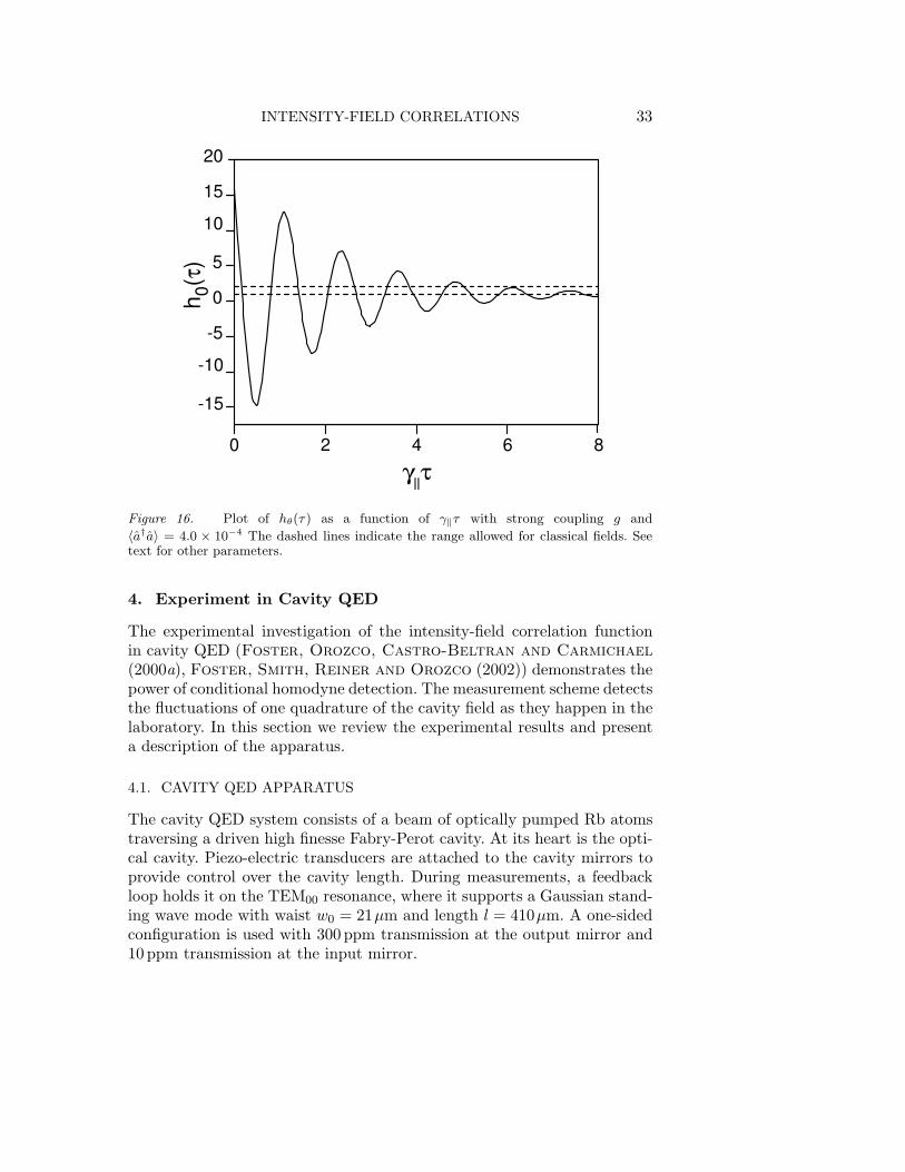
violations of the inequality from Eq. (15), both above (hθ(τ) > 2) and below(hθ(τ) < 0). For the ordinary OPO, only the former is true. Fig. 15ii plotshθ(τ) for weak coupling (g/γ = 0.1, g/κ = 1.0), with spontaneous emissiondominant over cavity decay (κ/γ = 0.1) and there are only violations above,as in the ordinary OPO. Fig. 16 shows results of the correlation function(hθ(τ) in the regime of strong coupling: (g/γ = 5.0; g/κ = 10.0), there arelarge violations of the Schwartz inequality Eq. (15), both above and below,with the appearance of vacuum-Rabi oscillations.

The intensity-field correlation functions for transmitted fields of a two-level atom in an optical parametric oscillator in the weak field limit behavesessentially as a cavity QED system where an occasional pair of photons ap-pears in the cavity and interacts with the system. For the intensity-fieldcorrelation function, which is essentially a quadrature field measurementconditioned on a photon detection, the system shows violations of the clas-sical Schwartz inequality (Eq. (15)). Unlike the OPO without a two-levelatom the system violates the upper and lower bounds over a wide range ofparameters. Vacuum-Rabi oscillations appear for large Jaynes-Cummingscouplings (g > κ, γ⊥). The inequality is violated from below only in theweak coupling regimes, and both above and below in the strong couplingregime. This is due in part to the field being π out of phase with the driv-ing field. The nonclassical behavior tends to go away as the driving fieldis increased (i.e. more photons are present) or as atoms are added to thesystem.


0 4

-15

-5

0

5

15

20

2 6 8

h 0(τ

)

-10

10

γ||τ

Figure 16. Plot of hθ(τ) as a function of γ‖τ with strong coupling g and

〈a†a〉 = 4.0 × 10−4 The dashed lines indicate the range allowed for classical fields. Seetext for other parameters.

4. Experiment in Cavity QED

The experimental investigation of the intensity-field correlation functionin cavity QED (Foster, Orozco, Castro-Beltran and Carmichael(2000a), Foster, Smith, Reiner and Orozco (2002)) demonstrates thepower of conditional homodyne detection. The measurement scheme detectsthe fluctuations of one quadrature of the cavity field as they happen in thelaboratory. In this section we review the experimental results and presenta description of the apparatus.

4.1. CAVITY QED APPARATUS

The cavity QED system consists of a beam of optically pumped Rb atomstraversing a driven high finesse Fabry-Perot cavity. At its heart is the opti-cal cavity. Piezo-electric transducers are attached to the cavity mirrors toprovide control over the cavity length. During measurements, a feedbackloop holds it on the TEM00 resonance, where it supports a Gaussian stand-ing wave mode with waist w0 = 21µm and length l = 410µm. A one-sidedconfiguration is used with 300 ppm transmission at the output mirror and10 ppm transmission at the input mirror.


An effusive oven, 35 cm from the cavity, produces a thermal beam of Rbatoms in a chamber pumped by a large diffusion pump operated at typicalpressures of 1× 10−6 Torr. The oven is heated to ≈ 430K± 0.1K with thehelp of computer controlled feedback. Final collimation is provided by a70µm slit on the front of the cavity holder. The cavity is surrounded by aliquid nitrogen cooled Cu sleeve to reduce the background atomic vapor, asthe presence of too much background destroys the observed correlations.

The excitation source is a Verdi 5 pumped titanium sapphire (Ti:Sapph)laser, a modified Coherent 899-01. The primary laser beam is split into asignal beam and auxiliary beams for laser frequency locking, cavity lock-ing, and optical pumping. All beams are on resonance with the 5S1/2, F =3 → 5P3/2, F = 4 transition of 85Rb at 780 nm. The atoms are opticallypumped into the 5S1/2, F = 3,mF = 3 state in a 2.5Gauss uniform mag-netic field applied along the axis of the cavity using the appropriate circularpolarization of the pumping light.

The cavity is locked with a Pound-Drever-Hall scheme. During data col-lection, the laser beam traverses a chopper wheel which alternately passesthe lock beam and opens the path from the cavity to the photon countingdetectors at ≈ 1.1kHz. Polarizing optics separate the signal from the lock.The signal beam is directed to the correlator. Between 50 and 85% of thesignal emitted from the cavity is sent to the BHD. The remaining 50 to 15%of the signal goes to the avalanche photodiodes. The choice is guided byexperimentally finding the best signal to noise ratio after averaging some60, 000 samples.

The three rates governing the atom-cavity coupling, cavity decay, andatomic decay in the cavity QED apparatus are (g, κ, γ⊥)/2π = (12, 8, 3) MHz,which yield C1 = 3 and n0 = 0.08, placing the experiment in the strongcoupling regime of cavity QED. The measurements are carried out with anaverage intracavity field less than that of one photon.

4.2. CONDITIONAL HOMODYNE DETECTOR

Measurement of the intensity-field correlation requires a homodyne mea-surement of the signal to be made correlated with photon detections. Amodified Mach-Zehnder interferometer was implemented to perform themeasurement. Fig. 17 shows a schematic of the interferometer and its in-tegration with the cavity QED apparatus. Light enters the Mach-Zehnderinterferometer, driving the cavity QED system on one arm and provid-ing a local oscillator (LO) for the BHD on the other (Yuen and Chan(1983a),Yuen and Chan (1983b)). A fraction of the signal is directed tothe BHD and the remainder is sent to the intensity detector (avalanchephotodiode APD). The photocurrent from the BHD is proportional to the


ATOMS

FIELD

INTENSITY

SIGNAL

LOCAL OSCILLATOR

AVALANCHE PHOTODIODE

CORRELATOR

TRIGGER

PHOTOCURRENT

+_

BALANCED HOMODYNE DETECTOR

CAVITYLIGHT

Figure 17. Schematic diagram of the cavity QED experimental setup.

LO-selected quadrature amplitude of the signal field. Photon detectionsat the APD are correlated with the BHD photocurrent to measure theintensity-field correlation function via Eq. (23). We discuss each compo-nent of the measurement in the following.

4.2.1. Mach-Zehnder InterferometerThe Mach-Zehnder interferometer is used to separate the laser into a localoscillator and a signal beam which, although they follow separate paths,maintain a constant relative phase. Control of the relative phase is criticalfor the measurement. It is achieved by adjusting the path difference of thetwo arms with a piezo-actuated mirror and actively stabilizing the interfer-ometer length with a feedback system. The stabilization uses a thermallystabilized He-Ne laser (λ = 633nm) or diode laser (λ = 640nm) locked us-ing FM sidebands to an Iodine cell. The cavity QED system is transparentto the red wavelengths, but they form fringes at the Mach-Zehnder output.An edge filter separates the 780nm and red wavelengths at the output.The MZ length is continually adjusted so such that it sits at a red fringemaximum or minimum. A phase change may be introduced by locking thelength to different red fringes. In this way the IR phase can be adjusted insteps of δθIR = 146 = (180 × 633/780). There is also an optical path de-lay that can be mechanically adjusted to bring the IR and red in phase at


a particular fringe.

4.2.2. Amplitude DetectorsThe combined signal and LO field is directed to a pair of biased siliconphotodiodes configured as a BHD. The AC coupled current from the pho-todiodes is amplified and subtracted to allow common mode rejection oflocal oscillator intensity noise (technical noise). The current from each de-tector first passes through a bias T which filters DC components below100kHz. The DC component provides a direct measure of the local oscilla-tor current.

4.2.3. Intensity DetectorsThe intensity detectors are arranged as a photon correlator consisting of twoavalanche photodiodes (APD) behind an unpolarized 50/50 beam splitter.The detectors have a quantum efficiency of 50%, a dark count rate of lessthan 50Hz, and a 30ns dead time. The detector electronics produce a TTLpulse for each photon detection, a copy of which goes to a counter thatmeasures the photon count rate of each APD. These rates yield the meanintensity of the light emitted from the cavity after correcting for efficienciesand linear losses.

4.2.4. Correlator Data AcquisitionThe homodyne current is sampled with a digital oscilloscope triggered byphoton detections registered at the APDs. The trigger is produced by theapparatus used elsewhere for intensity correlation measurements (Foster,Mielke and Orozco (2000b)). Instead of correlating the signals from theAPDs, for the intensity-field correlation the two signals are combined in alogical OR. The digital oscilloscope samples the BHD photocurrent over a500 ns window at 2 Gs/s with an 8 bit analog to digital (A/D) converter.It performs a summed average of the triggered samples. Typically up to5× 104 samples are taken.

4.3. MEASUREMENTS

The saturation photon number n0 in the experiment is less than one andhence the observed fluctuations are associated with the emission of a sin-gle conditioning photon. Fig. 18 shows data taken at an intracavity inten-sity n/n0 = 0.30, corresponding to a mean intracavity photon number of0.027. The data is in the low intensity regime. The trace on the left is theunormalized correlation function H(τ); it shows non-classical behavior, vi-olating the bound of Eq. (15), as the correlation has a minimum at τ = 0.On the right is its FFT, which in accord with Eq. (10) is proportionalto the spectrum of squeezing. The squeezing spectrum shows a dip at the


-200 -100 0 100 200

-40

-20

0

20

0 20 40 60

-2

0

2

Ω/2π (MHz)

FFT(

H(τ

))

(µA

/MH

z)

τ (ns)

H(τ

) AC

(µ

A)

i ii

Figure 18. i Conditional field (unnormalized) at low Intensity (n/n0 = 0.3) FieldCorrelation and ii its Fast Fourier Transform.

vacuum Rabi frequency Ω0. There is qualitative agreement with the pre-diction of Fig. 6, although the data is not normalized as would be requiredfor a quantitative comparison. The continuous line fitted to the FFT hasthe functional form predicted by the low intensity theory (Reiner, Smith,Orozco, Carmichael and Rice (2001)).

The BHD measures the interference between the local oscillator andthe emitted cavity field, which depends on their relative phase (Eq. (6)).A comparison of the conditionally averaged AC coupled photocurrent fortwo different local oscillator phases is shown in Fig. 19. When the relativephase is changed by 146 ≈ 180 (see Sect. 4.3.1) the sign of the interferencechanges. The normalization of these raw results is discussed in detail in thenext section. Notice, however, that even without the normalization, thevalue of the field at τ = 0 in Fig. 19i is clearly smaller than its steady-state value. This is further evidence of a non-classical field, since it violatesthe lower bound of Eq. (15). This nonclassical feature demonstrates thatthe field fluctuations are anticorrelated in a similar way to the intensityin photon antibunching. Rather than seeing random field fluctuations, wesee explicit evidence of the projection of the polarization field out of phasewith the steady-state intracavity field.

4.3.1. NormalizationThe correlation function defined by Eq. (8) is normalized to the mean field;therefore, obtaining the proper normalization calls for precise knowledge ofthis field. As the detection system is AC coupled, the mean field must bedetermined in some indirect manner. In practice, the proper DC level andnormalization has been determined by comparing the expected shot noiseafter averaging with the measured noise in the data. In this way, knowledge


-50

0

50

AC

Pho

tocu

rren

t (m

A)

i ii

25

-25

-100 0 100

τ(ns)50 -50 -100 0 100

τ(ns) 50 -50

Figure 19. Plots i and ii are unnormalized homodyne averages with a phase differenceof 146.

of the averaging procedure allows the normalized correlation function to beextracted.

The noise amplitude for the normalized correlation function is given by

δh =1

2〈a〉√η2κ

√Bκ

2Ns, (61)

where, as in Sec. 2, Ns is the number starts, κ is the cavity bandwidth, B isthe detector bandwidth in units of the cavity bandwidth, η is the fractionof the output power sent to the BHD, and 〈a〉 is the mean intracavity field(no offset is used in this measurement). Assuming then that the data canbe scaled with two constants, Ξ and Υ, such that

h(τ) = Ξhexpt(τ) + Υ, (62)

the normalization of h(τ) requires that

Ξhexpt(∞) + Υ = 1. (63)

To determine Ξ we note that Ξδhexpt = δh, and then assuming that the co-

herent transmission dominates the incoherent transmission (〈a〉 ≈√〈a†a〉),

Eq. (61) yields

Ξ ≈ 14δhexpt

√B

〈a†a〉ηNs. (64)

Υ is then recovered from Eq. (63). Aside from the reasonable assumption,this method determines the scaling from quantities measured in the exper-iment. The number of starts is recorded on the digital oscilloscope. The in-tracavity intensity and η are obtained from the measured flux at the APDs,


and the detection bandwidth is determined by the 70 MHz low pass filter.The noise amplitude δhexpt is determined by taking the standard deviationof the unnormalized data.

A second approach to the normalization of h(τ) uses the knowledgethat the normalized field correlation is the square root of the intensitycorrelation g(2)(τ) in the weak field limit. This permits a DC level for theraw field measurement to be determined that properly scales the normalizedintensity-field correlation function. The approach is less reliable for theseparticular measurements, however, because the data is not strictly taken ina weak field regime.

Finally, one might determine the normalization by calculating the DCfield expected from the measured photon flux. From the measured flux, theexpected DC voltage level can be calculated. Adding this level and dividingthe total by the same mean level normalizes the correlation data to give along-time mean of unity.

The difference between the first method of normalizing, on the basis ofthe expected noise, and the other two, is that it only includes the fractionof light directed to the BHD, without including the signal LO overlap,quantum efficiency, and additional losses. The first method of normalizationwas employed for the results presented here.

As an example of the normalized results, Fig. 20 shows h(τ) for a largerintracavity intensity (n/n0 = 1.2). The dashed area in the figure marks thelimits from the Schwartz inequalities in Eq. (15) and Eq. (18). The field isclearly non-classical. It is interesting to note that the intensity-intensity cor-relation function for an input intensity within 10% of that used to obtainFig. 20 shows only classical fluctuations, in the form of significant pho-ton bunching (Foster, Orozco, Castro-Beltran and Carmichael(2000a)). Note that in comparison with Figs. 18 and 19 a significant back-ground has appeared. Qualitatively the correlation function agrees withthat in Fig. 10i, where the stronger driving field causes many spontaneousemissions which interrupt the oscillatory evolution of the system back to thesteady state. Reiner, Smith, Orozco, Carmichael and Rice (2001)study the effects of spontaneous emission in greater detail.

4.3.2. Spectrum of SqueezingThe Fourier transform of the normalized intensity-field correlation function,when multiplied by the source photon flux, gives the spectrum of squeezing(Eq. (10)). Thus, a single time domain measurement of the fluctuationof the field quadrature amplitude yields the entire spectrum of squeezingin the frequency domain. The spectrum in Fig. 21 is computed from thenormalized data of Fig. 20. Since the data contains noise, the time serieswas first symmetrized and then ordered in a one-dimensional array, with


-100 0 1000.9

1.0

1.1

1.2

τ (ns)

h 0o(

τ)

Figure 20. Measured normalized field correlation for an in-phase field in cavity QED.N=13 and n/n0 = 1.2. The dashed region is classically allowed.

the positive times appearing first followed by the negative times in reverseorder. The real part of the fast Fourier transform (FFT) is then taken,and multiplied by the time resolution of the data and twice the flux F(Eq. (11)), as determined from the measured rates at the APDs and theirmeasured efficiencies.

There is squeezing below the standard quantum limit (or the shot noiselevel) at the vacuum Rabi frequency Ω0. The magnitude at this frequencyis ≈ 5%. The positive peak at zero is primarily caused by the spontaneousemission noise (Reiner, Smith, Orozco, Carmichael and Rice (2001))and is in qualitative agreement with the result displayed in Fig. 10.

The measurements of the cavity QED system show that the detectionof a photon projects the system into a quantum state that evolves in timewith a well-defined phase (relative to the mean field). The conditional ho-modyne detection uses this feature to observe the evolution of the fieldfluctuation; by triggering the collection of data from the BHD on a pho-


Ω/2π (MHz)0 100

-5

0

5

10

15S

(Ω,θ

=0o )

x 102

20 40 60 80

Figure 21. Squeezing Spectra for cavity system with n/n0 = 1.2, and source fluxF = 10.9× 106 photons/sec.

ton detection, one recovers the subphoton field fluctuation from the largeshot noise background. The time-domain measurement provides the infor-mation required to construct the full spectrum of squeezing in an efficiencyindependent manner.

5. Equal-Time Cross- and Auto-Correlations

We review in this section a series of theoretical and experimental papersthat have studied conditional homodyne measurements at equal times, thismeans they do not look at the dynamics of the state as we have shown inprevious sections, but they show very interesting results that demonstratethe quantum nature of conditional states of the electromagnetic field.

The entanglement available on the output field produced in the paramet-ric down-conversion process has been exploited thoroughly to perform stud-ies of conditional quantum measurements. Yurke and Stoler (1987) pro-posed a cross correlation measurement, a conditional measurement, of the


quadrature of the electromagnetic field as a way to measure the ampli-tude probability distributions for photon-number operator eigenstates. Ban(1996) studied the photon statistics of conditional output states with a pho-ton counting detector at one output of a beam splitter and a homodynedetector at the second output of the beam splitter for different input fields.This treatment is equivalent to h(0) the auto-correlation between the in-tensity and the field of a signal beam and enables the author to study theMandel Q factor of the conditional output state in detail.

More recently Crispino, Giuseppe, Martini, Mataloni and Kana-toulis (2000), and Lvovsky, Hansen, Aichele, Benson, Mlynekand Schiller (2001) performed a cross correlation measurement and ap-plied tomographic methods to reconstructed the Wigner distribution for aone photon state using conditional homodyne detection. Fiurasek (2001)studied the photon statistics conditioned on the homodyne detection in asimilar system. Resch, Lundeen and Steinberg (2002a) and Resch,Lundeen and Steinberg (2002b) used intensity-field cross-correlationsfor measurements of conditional coherence in prepared quantum states andto implement a conditional phase switch at the single photon level.

5.1. CROSS-CORRELATIONS

We generalize the definition of the unormalized correlation function Hθ(τ)in Eq. 4 to allow two different modes, allowing us to cross correlate theintensity fluctuations on one mode with the field fluctuations of anothermode:

Hθ(τ)i,j =〈 : Si(t)Dj(t + τ) : 〉

〈Si〉+ ξ(t). (65)

where the labels i and j refer to two different modes. The normalizationproceeds in the same way as in section 2 so we can now talk about theconditional field on mode j given a photon detection on mode i. This isuseful in the case of the two entangled modes of a parametric down conver-tor. (See Fig. 22). The connection with squeezing given by Eq. (10) for theauto-correlation h(τ) is not valid in the case of the cross-correlation h(τ)i,j .

5.1.1. Proposal for measuring the amplitude probability of a Fock stateYurke and Stoler (1987) present measurement strategy to obtain theprobability distribution of an n photon Fock state. They suggest the highlycorrelated process of parametric down conversion where the number of pho-tons counted by a photodetector in the idler beam during a coherence timecould be used to gate a homodyne detector in the signal beam. The in-tegrated output of the homodyne detector over a coherence time is onlyrecorded when an m-photon wave packet enters its input port. In this way


conditionalphotocurrent

homodynedetector

pulsed laser doublerdownconverter

local oscillator

triggerdetector

andsignal

Figure 22. Simplified apparatus for measurement of the cross-correlation H(0)i,j inparametric down conversion.

it is possible to map out the probability distribution for a field-amplitudecomponent of a number-operator eigenstate.

They propose to measure the cross-correlation or conditional amplitudeH(τ)i,j in a parametric down converter, where the idler beam is the modei, and the signal beam is the mode j. Their proposal does not show away to normalize the correlation function, as is suggested in Section 2 ofthis review by adding a coherent offset (See Fig. 1). They suggest thatthis conditional measurement could be used for the same purpose on othernon-linear sources that produce non-classical light.

5.1.2. State Reconstruction of a Fock state and Quantum-OpticalCatalysis.Crispino, Giuseppe, Martini, Mataloni and Kanatoulis (2000) andLvovsky, Hansen, Aichele, Benson, Mlynek and Schiller (2001) havereconstructed the quantum state of optical pulses containing single photonsusing the method of phase-randomized pulsed optical homodyne tomogra-phy. The method they apply is very similar, but we review here in moredetail the experiment of Lvovsky, Hansen, Aichele, Benson, Mlynekand Schiller (2001). They prepare a single-photon Fock state |1〉, in awell-defined spatiotemporal mode, using conditional measurements on pho-ton pairs born in the process of parametric down-conversion following theoriginal suggestion by Yurke and Stoler (1987).

A single-photon counter is placed into one of the emission channels(labelled trigger in Fig. 22) to detect photon pair creation events and totrigger the readout of a homodyne detector placed in the other (signal)channel. (See Hansen, Aichele, Hettich, Lodahl, Lvovsky, Mlynekand Schiller (2001) for a description of their detector).

The signal beam as shown in Fig. 22 is not an optical beam in thetraditional sense. The down-converted photons are in fact emitted randomlyover a wide solid angle. The optical mode of the signal state is usable when


bias | α >

intensity

conditional photocurrenthomodyne

detector

pulsed laser doublerdownconverter

local oscillator

triggerdetector

andsignal

and

Figure 23. Simplified scheme of the experimental setup for H(0) of a Fock State withthe help of an offset field.

a photon of a pair hits the trigger detector and is registered. Once theapproximation of the Fock state is prepared, it is subjected to balancedhomodyne detection Yuen and Chan (1983a), Yuen and Chan (1983b).

They obtain a probability distribution of the phase-averaged electricfield amplitudes with a non-Gaussian shape. They then reconstruct theangle-averaged Wigner function from this distribution that shows a dipreaching classically impossible negative values around the origin of thephase space.

This is an intensity-field cross-correlation at equal times (see Eq. (65)),here presented as a conditional measurement. The evolution of the para-metric down conversion process is very fast so they do not get the timedependence. They do not have an average field to normalize the correla-tion function that they measure, so the results are not independent of thequantum efficiency of the detectors.

Lvovsky and Shapiro (2002) have used the equal time intensity-fieldcross-correlations to measure and characterize non-classical light. Anotheruse of the cross-correlation between the intensity of one mode and the fieldof another as done in the work described above is the work of Fiurasek(2001). Instead of conditioning on the intensity fluctuations (photodetec-tion) the paper proposes to use the homodyne signal to condition the pho-todetections. The photodetector only counts if the absolute value of themeasured idler quadrature lies inside a certain range. The conditioned gen-erated signal is sub-Poissonian.

As a follow up of their previous cross-correlation work Lvovsky andMlynek (2002) use a intensity-field cross-correlator to measure the con-ditional field of a single photon. (See Fig. 23 for a schematic of their ap-paratus). They prepare the single photon through the parametric downconversion process with a conditional measurement and then they use the


Fock state as the “source” (See Fig. 1) for their intensity-field correlator.Since the Fock state does not have a steady state amplitude, they add acoherent bias field to do the auto-correlation measurement Hθ(0) at equaltimes.

Lvovsky and Mlynek (2002) show that with the appropriate choiceof offset, they can prepare and characterize a coherent superposition statest|0〉 + α|1〉 of the electromagnetic field by conditional measurements on abeam splitter. The single photon plays the role of a catalyst: it is explicitlypresent in both the input and the output channels of the interaction yetfacilitates generation of a nonclassical state of light. Although their mea-surement does not give the full time dependent intensity-field correlationfunction, since they can obtain the value at τ = 0, from the Fourier Trans-form relations presented in section 2 (see Eq. (12)) it is possible to obtainthe integrated spectrum of squeezing for this Fock state.

6. Quantum Measurements and Quantum Feedback

The intensity-field correlation function has introduced a new way to an-alyze and study the non-classicality of the electromagnetic field. It doesthat mainly through the two Schwartz inequalities in Eqs. 15, 18. Recentworks by Wiseman (2002) and Carmichael (2003) show that the condi-tional homodyne detection, key to measuring h(τ), has further implicationsin the quantum theory of measurement through its relationship with theweak measurements of Aharonov, and in distinguishing qualitatively be-tween vacuum state squeezing and the mere squeezing of classical noise.Carmichael (in press)has used the connection between the intensity-fieldcorrelation and the particle-wave aspects to further elucidate this importantquestion. Conditional measurements and quantum feedback are intimatelyrelated Wiseman (1994). The last part of this section presents a proposalto use CHD in quantum feedback to modify the the response of a cavityQED system.

6.1. WEAK MEASUREMENTS

We review the main ideas behind a weak measurement and follow Wiseman(2002) in developing the connection between h(τ) and weak measurements.A weak measurement is one that minimally disrupts the system, while con-sequently yielding a minimal amount of information about the observablemeasured (Aharonov, Albert and Vaidman (1988)). For a given initialsystem state, the ensemble average of weak-measurement results is the sameas for strong i.e., projective measurement results. Where weak measure-ments are interesting is when a final as well as an initial state is specified.Here the final state is the result of a second measurement (a strong one), so


that the ensemble average is taken over a postselected ensemble, in whichthe desired result for the final measurement was obtained.

A homodyne measurement gives a current proportional to the expecta-tion value of the quadrature operator and so conditions the system state.The photon counting also gives a continuous measurement that is weak inthe sense that the average change in the conditioned system in time δt isof order δt, as seen in quantum trajectories (Reiner, Smith, Orozco,Carmichael and Rice (2001)). However, unlike homodyne detection,sometimes the change is great, there is a quantum jump and either thesystem changes state or continues its evolution.

Looking at the negative time side of the correlation function it is possibleto see that this is a weak value preselected by the system being in itsstationary state, and postselected on the photon detected at time τ = 0.The measurements of the correlation function, as a function of time showsthe dynamics of a weak value (quadrature of the electromagnetic field)over time. The strangeness of the weak values in this experiment is notsurprising, since the conditions set by Aharonov, Albert and Vaidman(1990) are fulfilled. That is, the postselection is done on a rare event, thedetection of one photon rather than zero photons.

The formulation of the quantum trajectory has to have the influence ofthe homodyne detection to be consistent and describe the times before thedetection of a photon. Wiseman (2002) shows that h(τ), the intensity-fieldcorrelation function reduces to a form as simple as that originally derivedby Aharonov, Albert and Vaidman (1988)

6.2. VACUUM STATE SQUEEZING VERSUS SQUEEZED CLASSICALNOISE

It is apparent from Eqs. (9) and (10) that conditional homodyne detectionoffers a somewhat different view of squeezed light than the conventionalsqueezing measurement. Certainly, the latter is usually carried out in thefrequency domain, but this difference is not important. In both cases wehave a Fourier relationship between frequency and time of the sort givenin Eq. (11). The important difference is that in the conventional measure-ment, the relevant temporal correlation function is the direct autocorre-lation of the current, i(t), from the balanced homodyne detector, whichis calculated from a symmetrically ordered quantum average, rather thanthe normal-ordered average of Eq. (9). The difference is a direct mani-festation of conditioning, and from it, it follows that whereas a conven-tional homodyne measurement distinguishes quantitatively between vac-uum state squeezing and squeezed classical noise, conditional homodynedetection distinguishes quantum from classical squeezing in a qualitativeway (Carmichael (2003)).


Physically, in any realistic example, squeezing is restricted to a finitebandwidth, outside of which the field fluctuations are not squeezed. Forvacuum state squeezing, the unsqueezed fluctuations appear as shot noiseon i(t), the shot noise commonly being interpreted as a manifestation of thevacuum fluctuations of the measured field. If, in addition, this field carriesbroadband classical noise, the unsqueezed classical fluctuations also add tothe fluctuations of i(t). Thus, in a conventional squeezing measurement,unsqueezed classical noise and shot noise contribute to the autocorrelationof i(t). In conditional homodyne detection, by comparison, only the classi-cal noise contributes; the shot noise is eliminated; through the conditionalsample average, the term ξ(τ) in Eq. (9) is reduced (in the ideal limit) tozero.

To illustrate the comparison, we consider the squeezing of broadbandclassical noise, as depicted in Fig. 24i. Classical noise of bandwidth (halfwidth)Bcκ = 15κ is squeezed by a sub-threshold degenerate parametric oscilla-tor over the bandwidth κ. Fluctuations on the squeezed quadrature of Eout

are then measured using either conventional homodyne detection or condi-tional detection; the detection bandwidth is Bdκ = 25κ. Figures 24ii and iiishow simulated results for the direct autocorrelation of the homodyne cur-rent, and thus provide the time-domain view of a conventional squeezingmeasurement. The presence of squeezing is evident from the broad nega-tive dip, while fluctuations outside the squeezing bandwidth produce thenarrow spike around τ = 0. In frame ii, this spike is contributed to by bothclassical fluctuations and shot noise. The shot noise alone contributes inframe iii; here the height of the spike is correspondingly reduced.

For comparison, Fig. 25 displays simulated results of conditional ho-modyne detection. In this case, there is no shot noise contribution to thecentral spike. The spike shrinks and eventually disappears as the classicalnoise level is decreased. A central spike in hθ(τ) is therefore a qualitativeindicator of the squeezing of classical, as opposed to vacuum state noise.

Carmichael (2003) has also investigated to what extent stochasticelectrodynamics is able to reproduce this distinction between classical andvacuum noise squeezing. He finds that the results of Fig. 25 are reproduced,but with an additional background contribution generated by “starts” in-duced by the explicit vacuum noise (unphysical dark counts). In relatedwork, triple correlations of the quadratures of the electromagnetic fieldhave been used by Drummond and Kinsler (1995), Kinsler (1996),Chaturvedi and Drummond (1997), and Pope, Durmmond and Munro(2000) to investigate differences between the predictions of stochastic elec-trodynamics and quantum mechanics. They compare the former with thepositive P representation and also focus their attention on the parametricoscillator.


filteredclassical noise

bandwidth Bcκ

E out

squeezerbandwidth κ

i

-6 0

0

4

κτ6

iii

i(0)i(

τ)

-6 0

0

4

8

6κτ

ii

i(0)i(

τ)

Figure 24. i Sketch of the degenerate OPO squeezer with broadband classical noise input.Under conventional homodyne detection of the field Eout [ii and iii], the autocorrelation ofthe homodyne current reveals nonsqueezed fluctuations over a wide bandwidth (centralspike) and a narrow bandwidth of squeezed fluctuations (negative dip): for a classicalnoise bandwidth Bcκ = 15κ, detection bandwidth Bdκ = 25κ, and classical noise photonnumbers (in the degenerate OPO cavity) of ii nc = 0.2 and iii nc = 0; the degenerateOPO squeezer is operated at 40% of threshold.

6.3. APPLICATION OF Hθ(τ) TO QUANTUM FEEDBACK

Most quantum feedback proposals use the BHD photocurrent to modify thedrive acting on a quantum system. The goal of such feedback can vary fromreducing out-of-quadrature noise (Tombesi and Vitali (1995)) to modify-ing the system dynamics (Wang and Wiseman (2001)). All these propos-als rely on continuous feedback. Doherty and Jacobs (1999) showed thatone can improve these schemes with knowledge of the conditioned state. Arecent experiment by Smith, Reiner, Orozco, Kuhr and Wiseman(2003) shows the success of quantum feedback in a strongly coupled systemthrough conditional intensity measurements.

We consider adding feedback to the single atom cavity QED system (Seesection 3.2 for theoretical details). A photon leaves the cavity which initiatesa fluctuation. Conditioning the BHD detectors to observe this fluctuationalso creates the opportunity to apply feedback.

The dynamics of this system, once the detection of the photon is made,


0.8

0.9

1.0

1.1

1.2

hy

0.8

0.9

1.0

1.1

1.2

hy

0.8

0.9

1.0

1.1

1.2

hy

0.2

0.6

1.0

1.4

1.8 h

y

-6 0 6κτ

i

-6 0 6κτ

iii

-6 0 6κτ

-6 0 6κτ

iv

ii

Figure 25. Broadband classical noise squeezing under conditional homodyne detection.The correlation function hY (τ), with Y the squeezed quadrature, is plotted for the pa-rameters of Fig. 24 and classical noise photon numbers (in the degenerate OPO cavity)of i nc = 0.2, ii nc = 0.1, iii nc = 0.05, and iv nc = 0.

are governed by the regression to steady state of the field. That for weakfields reduce in the Optical Bistability notation of Lugiato (1984) to:

x = κy + gp− κx + Gx

p = −gx− γ⊥p. (66)

where y is the normalized intracavity field in the absence of atoms (pro-portional to the drive), x the intracavity field in the presence of atoms, p isthe atomic polarization, and G quantifies the strength of the field feedback.

The intensity-field correlator measures the conditioned BHD photocur-rent,

i(t) =√

2κη〈x(t)〉+ ξ(t), (67)


ATOMS

SIGNAL

LOCAL OSCILLATOR

AVALANCHE PHOTODIODE

CORRELATOR

TRIGGER

PHOTOCURRENT

+_

BALANCED HOMODYNE DETECTOR

CAVITY

LIGHT

ELECTRO OPTICAL MODULATOR

i(t 1)i(t2)

i(t3)t2 t3 t1 < <MODULATOR

DRIVER

FEEDBACK CURRENT

Figure 26. Schematic of the feedback apparatus. The running average is feedback toreduce the contribution of the shot noise component.

which is proportional to the intra-cavity field and contains shot noise (ξ(t)).We propose modulating the amplitude of the driving laser with the con-ditioned BHD photocurrent. This modifies the system Hamiltonian HS toinclude:

Hfb = Gi(t)(a− a†

). (68)

We improve this feedback by averaging away the shot noise contributionin Eq. (68).

H(N, τ)fb =∑Ns

j=1 λic(tj + τ)Ns

(69)

Figure 26 presents a suggestion of how the intensity-field correlator inthe experiment of Foster, Orozco, Castro-Beltran and Carmichael(2000a) would be modified to apply quantum feedback. Photons arrive atthe avalanche photodiode at different times, t1, t2 and t3. These are wellseparated to show the reduction in shot noise with consecutive averages.

Figure 27 shows the conditioned field evolution of a single maximallycoupled stationary atom in cavity QED without and with the feedbackprotocol defined by Eq. (68) set to enhance the vacuum Rabi oscillations ofthe system. The evolution has been maintained well beyond the limits set by(κ+γ⊥)/2. The plot is the result 10,000 averages to reduce the contributionfrom the shot noise.


-9 -6 -3 0 3 6 9gτ

i

-400

-300

-200

-100

0

100

200

300

400

h 0o(τ

)ii

-9 -6 -3 0 3 6 9gτ

Figure 27. Single atom cavity QED quantum conditioned field evolution: i withoutfeedback, and ii with feedback. (g, κ, γ⊥, Γ,G)/2π = (38.0, 8.7, 3.0, 100, 3.5) MHz.

7. Conclusion and Outlook

Future studies may try to map out a full phase space picture of the condi-tional field as it evolves in time. This would involve sampling the field atvarious phases and performing some type of tomographic reconstruction toarrive at a quasi-probability distribution (Leonhardt (1997)).

The conditional homodyne technique may have more general applicationto studying other sources both classical and non-classical since the informa-tion obtained through this intensity-field correlation approach complementsand synthesizes that coming from intensity-intensity correlations (particleaspect) and squeezing (wave aspect).

Acknowledgments

Work supported by NSF and NIST.

References

Aharonov, Y., Albert, D. and Vaidman, L. (1988), Phys. Rev. Lett. 60, 1351.Aharonov, Y., Albert, D. and Vaidman, L. (1990), Phys. Rev. A 41, 11.Bachor, H. A. (1998), A Guide to Experiments in Quantum Optics, Wiley-VCH, New

York.Ban, M. (1996), J. Mod. Opt. 43, 1281.Banaszek, K. and Wodkiewicz, K. (1996), Phys. Rev. Lett. 76, 4344.Brecha, R. J., Rice, P. R. and Xiao, M. (1999), Phys. Rev. A 59, 2392.Brown, R. H. and Twiss, R. Q. (1956), Nature 177, 27.Carmichael, H. J. (1987), J. Opt. Soc. Am. B 4, 1588.Carmichael, H. J. (1993a), An Open Systems Approach to Quantum Optics, Lecture Notes

in Physics, Vol. 18, Springer-Verlag, Berlin.


Carmichael, H. J. (1993b), Phys. Rev. Lett. 70, 2273.Carmichael, H. J. (1999), Statistical Methods in Quantum Optics 1: Master Equations

and Fokker-Planck Equations, Springer-Verlag, Berlin.Carmichael, H. J. (2003), Submitted.Carmichael, H. J. (in press), Quantum fluctuations of light: a modern perspective on

wave/particle duality, in A. Thorndike, ed., ‘One Hundred Years of the Quantum:from Max Planck to Entanglement’, Chicago University Press, Chicago.

Carmichael, H. J., Brecha, R. J. and Rice, P. R. (1991), Opt. Commun. 82, 73.Carmichael, H. J., Brecha, R. J., Raizen, M. G., Kimble, H. J. and Rice, P. J. (1989),Phys.

Rev. A p. 5516.Carmichael, H. J., Castro-Beltran, H. M., Foster, G. T. and Orozco, L. A. (2000), Phys.

Rev. Lett. 85, 1855.Casimir, H. B. G. (1945), Rev. Mod. Phys. 17, 343.Chaturvedi, S. and Drummond, P. D. (1997), Phys. Rev. A 55, 912.Clemens, J. P., Rice, P. R., Rungta, P. K. and Brecha, R. J. (2000), Phys. Rev. A

62, 033802.Collett, M. J. and Gardiner, C. W. (1984), Phys. Rev. A 30, 1386.Collett, M. J. and Gardiner, C. W. (1985), Phys. Rev. A 32, 2887.Collett, M. J. and Loudon, R. (1987), J. Opt. Soc. Am. B 4, 1525.Crispino, M., Giuseppe, G. D., Martini, F. D., Mataloni, P. & Kanatoulis, H.(2000),

Fortschr. Phys. 48, 589.Deng, H., Erenso, D., Vyas, R. and Singh, S. (2001), Phys. Rev. Lett. 86, 2770.Denisov, A., Castro-Beltran, H. M. and Carmichael, H. J. (2002), Phys. Rev. Lett.

88, 243601.Doherty, A. C. and Jacobs, K. (1999), Phys. Rev. A 60, 2700.Drummond, P. D. and Kinsler, P. (1995), Quantum Semiclass. Opt. 7, 727.Fiurasek, J. (2001), Phys. Rev. A 64, 053817.Foster, G. T., Orozco, L. A., Castro-Beltran, H. M. and Carmichael, H. J. (2000a), Phys.

Rev. Lett. 85, 3149.Foster, G. T., Mielke, S. L. and Orozco, L. A. (2000b), Phys. Rev. A 61, 053821.Foster, G. T., Smith, W. P., Reiner, J. E. and Orozco, L. A. (2002), Phys. Rev. A

66, 033807.Glauber, R. J. (1963a), Phys. Rev. 131, 2766.Glauber, R. J. (1963b), Phys. Rev. Lett. 10, 84.Glauber, R. J. (1963c), Phys. Rev. 130, 2529.Graham, R. (1971), Springer Tracts in Modern Physics Vol 66, 1st edn, Springer-Verlag,

Berlin.Graham, R. and Haken, H. (1971), Z. Phys. 243, 189.Hansen, H., Aichele, T., Hettich, C., Lodahl, P., Lvovsky, A. I., Mlynek, J. and Schiller,

S. (2001), Opt. Lett. 26, 1714.Jaynes, E. T. and Cummings, F. W. (1963), Proc. IEEE 51, 89.Jin, S. and Xiao, M. (1993), Phys. Rev. A 48, 1473.Jin, S. and Xiao, M. (1994), Phys. Rev. A 49, 499.Kimble, H. J. and Walls, D. F. (1987), J. Opt. Soc. Am. B 4, 1450.Kimble, H. J., Dagenais, M. and Mandel, L. (1977), Phys. Rev. Lett. 39, 691.Kinsler, P. (1996), Phys. Rev. A 53, 2000.Klein, M. J. (1955), Phys. Rev. 97, 1446.Leach, J., Strimbu, C. E. and Rice, P. (2003), Submitted.Leonhardt, U. (1997), Measuring the Quantum State of Light, Cambridge University

Press, Cambridge.Loudon, R. (1980), Rep. Prog. Phys. 43, 913.Loudon, R. and Knight, P. L. (1987), ‘Squeezed light’, J. Mod. Opt. 34, 709.Lugiato, L. A. (1984), Theory of optical bistability, in E. Wolf, ed., ‘Progress in Optics’,

Vol. XXI, North-Holland, Amsterdam, pp. 69–216.Lutterback, L. G. and Davidovich, L. (1997), Phys. Rev. Lett. 78, 2547.


Lvovsky, A. I., Hansen, H., Aichele, T., Benson, O., Mlynek, J. and Schiller, S. (2001),Phys. Rev. Lett. 87, 050402.

Lvovsky, A. I. and Mlynek, J. (2002), Phys. Rev. Lett. 88, 250401.Lvovsky, A. I. and Shapiro, J. H. (2002), Phys. Rev. A 65, 033830.Mandel, L. and Wolf, E. (1995), Optical Coherence and Quantum Optics, Cambridge

University Press, New York.Milburn, G. and Walls, D. F. (1981), Opt. Commun. 39, 401.Onsager, L. (1931), Phys. Rev. 37, 405.Paul, H. (1982), Rev. Mod. Phys. 54, 1061.Pope, D. T., Drummond, P. D. and Munro, W. J. (2000), Phys. Rev. A 60, 052108.Reiner, J. E., Smith, W. P., Orozco, L. A., Carmichael, H. J. and Rice, P. R. (2001), J.

Opt. Soc. Am. B 18, 1911.Resch, K. J., Lundeen, J. S. and Steinberg, A. M. (2002a), Phys. Rev. Lett. 88, 113601.Resch, K. J., Lundeen, J. S. and Steinberg, A. M. (2002b), Phys. Rev. Lett. 89, 037904.Rice, P. R. and Carmichael, H. J. (1988), J. Opt. Soc. Am. B 5, 1661.Siddiqui, S., Erenso D., Vyas R., and Singh S.(2003),Phys. Rev. A 67, 06380855.Slusher, R. E., Hollberg, L. W., Mertz, J. C., Yurke, B. and Valley, J. F. (1985), Phys.

Rev. Lett. 55, 2409.Smith, W. P., Reiner J. E., Orozco L. A., Kuhr S. and Wiseman H. M. (2002), Phys.

Rev. Lett. 89, 133601.Strimbu, C. E. and Rice, P. R. (2003), Submitted.Tolman, R. C. (1938), The Principles of Statistical Mechanics, Oxford University Press,

London.Tombesi, P. and Vitali, D. (1995), Phys. Rev. A 51, 4913.Tomita, K. and Tomita, H. (1973), Phys. Lett. A 46, 265.Tomita, K. and Tomita, H. (1974), Prog. Th. Phys. 51, 1731.Vogel, W. (1991), Phys. Rev. Lett. 67, 2450.Vyas, R. and Singh, S. (2000), Phys. Rev. A 62, 0338033.Wallentowitz, S. and Vogel, W. (1996), Phys. Rev. A 53, 4528.Walls, D. F. (1979), Nature 280, 451.Wiseman, H. M. (1994), Phys. Rev. A 49, 2133.Wang, J. and Wiseman, H. M. (2001), Phys. Rev. A 64, 063810.Wiseman, H. M. (2002), Phys. Rev. A 65, 032111.Yuen, H. P. and Chan, V. W. (1983a), Opt. Lett. 8, 177.Yuen, H. P. and Chan, V. W. (1983b), ‘Errata’, Opt. Lett. 8, 345.Yurke, B. and Stoler, D. (1987), Phys. Rev. A 36, 1955.

intensity-field correlations of non ... - umd physics

Documents