correlation-based data representation

Correlation-based Data Representation

Marc Strickert and Udo Seiffert

Leibniz Institute of Plant Genetics and Crop Plant Research GaterslebenBioinformatics Division

{stricker,seiffert}@ipk-gatersleben.de

Abstract. The Dagstuhl Seminar Similarity-based Clustering and itsApplication to Medicine and Biology (07131) held in March 25–30, 2007,provided an excellent atmosphere for in-depth discussions about the re-search frontier of computational methods for relevant applications ofbiomedical clustering and beyond. We address some highlighted issuesabout correlation-based data analysis in this seminar postribution. First,some prominent correlation measures are briefly revisited. Then, a focusis put on Pearson correlation, because of its widespread use in biomedicalsciences and because of its analytic accessibility. A connection to Euclid-ean distance of z-score transformed data outlined. Cost function opti-mization of correlation-based data representation is discussed for which,finally, applications to visualization and clustering of gene expressiondata are given.

Keywords. correlation, data representation, gradient-based optimiza-tion, clustering, neural gas, visualization, multi-dimensional scaling

1 Introduction

Data comparison is one of the most fundamental operations in data analysis.Comparisons are used to induce an ordering of data, which can be regardedas precursor to clustering, i.e. grouping of similar data. Although ordering andclustering can be defined as two stand-alone problems, there are many effortsto combine both tasks: self-organizing maps realize such a combination by vec-tor quantization (clustering) and mapping to a low dimensional grid (ordering);as another example, hierarchical clustering generates clustering trees, which areusually post-structured by means of leaf-ordering procedures. In addition, graph-ical data representations are frequently found in biomedical publications, such asprincipal component projections, for visually illustrating closeness (clustering)of reference data points and their arrangement (ordering) along axes of principalchanges, such as induced by time, probe concentrations, stress application, andso forth. Ordering of multi-dimensional data items, and likewise their centroidrepresentations, according to similarity is thus a non-trivial task, because the di-versity of complex orthogonal relationships needs to be reduced to lists or otherlow-dimensional structures that can be intuitively called ordered.

Dagstuhl Seminar Proceedings 07131Similarity-based Clustering and its Application to Medicine and Biologyhttp://drops.dagstuhl.de/opus/volltexte/2007/1134

2 M. Strickert, U. Seiffert

Relative and absolute distance sources can be identified for data comparisons.Relative distances are characterized by knowledge of an adjacency matrix,

for example, gradients between concentrations of chemical agents. Correspond-ing network nodes need not have a proper physical representation to which anabsolute measure is applicable; the network might be defined only by proximityrelationships between the nodes. If needed, an auxiliary physical representationof such proximity network can be obtained, for example, by multi-dimensionalscaling methods that embed proximities into a target vector space with fixeddimensionality, possibly Euclidean, for convenience. Such embedding is compu-tationally costly, though, and a loss of information is inevitable in many cases.This motivates direct functional methods for dealing with proximity data [1]which also facilitate comparisons of non-vector objects like strings or graphs.

Absolute distances provide a comparison of data items, here, vectors of fixeddimensionality. Although metrics, distances, and similarity measures differ intheir degree of mathematical strictness, there is some common sense about thebasic intention in clustering: maximum data similarities are sought, or, on thecontrary, minimum distances and dissimilarities. In such an intuitive manner,Minkowski metrics, the Malahanobis distance, and Kendall correlation are ex-amples of absolute ’distances’, although the mathematical definition of distanceis more stringent.

Since clustering results are depending only on the data, the data measure,and the computing method, the the data measure has to be chosen carefully. Inmany biological applications, correlation measures are preferred because of theirfavorable invariance properties: adding a constant offset to components of a datasample, or applying a multiplicative factor does not affect correlation. Such in-variance helps, up to a certain degree, to circumvent calibration issues connectedto measuring devices. As will be discussed, normalization does not always allowto boil down data for treatment with the standard Euclidean distance.

In the following, correlation measures will be briefly revisited, Pearson cor-relation will be considered in detail, and, connected to this, cost function basedoptimization for clustering and visual data screening will be presented.

2 Correlation Measures

In general, correlation quantifies the strictness of dependence of two vectors: ’themore of one amount, the more of the other’, corresponds to positive correlation,while negative correlation indicates ’the more of one, the less of the other’. Highabsolute correlation values, though, are no guarantee that two observations reallyinfluence one another. Correlations might be caused by spurious dependence,either mediated by a hidden factor controlling both, or simply by chance. Thisexplains, why ’measure of association’ is a misleading synonym of correlation.

Different types of correlation can be specified. For brevity, we refer to exist-ing literature and focus on the three most frequent ones [2]. These are Kendall’sTau [τ ], comparing occurrences of positive and negative signs of differences ofcomponents in two vectors; Spearman rank correlation, comparing rank order-

07131 – Dagstuhl Seminar Proceedings 3

ings, i.e. monotonic relationships, of the entries in two vectors; and Pearsoncorrelation which is a measure of linear correlation between real-value entriesof two vectors. The three measures yield numerical values in a range between-1, meaning negative correlation, and +1, meaning positive correlation; valuesaround zero indicate uncorrelatedness.

2.1 Kendall’s Tau [τ ]

The Kendall coefficient τ measures the strength of the common tendency oftwo d-dimensional vectors x = (xk)k=1...d and w = (wk)k=1...d in a very directmanner. Data pairs (xi, wi) and (xj , wj) are considered. If xi − xj and wi − wj

have the same sign, the pair is concordant, else it is discordant. The number ofconcordant pairs is C, the number of discordant pairs is D, for i < j in bothcases. Then

τ =C −D

d · (d− 1)/2describes the amount of bias towards concordant or discordant occurrences, nor-malized by the effective number of component pairs. Versions for handling tieddata are also available. For its fundamental counting statistics and its easy in-terpretation Kendall’s τ might be considered as favorable characterization ofcorrelation. However, the computing complexity is O(d2), i.e. quadratic in thenumber d of data dimensions. Also, τ does change in discrete steps as data rela-tionships change, which makes it difficult to use in optimization scenarios, suchas the optimum data representation task described below.

2.2 Spearman Rank Correlation

Another non-parametric correlation measure is obtained by calculating the nor-malized squared Euclidean distance of the ranks of xk and wk according to

ρ(x,w) = 1− 6d · (d2 − 1)

·d∑

k=1

(rnk(xk)− rnk(wk)

)2.

Ranks of real values ck are defined by rnk(ck) = | {ci < ck , i = 1 . . . d} |, whichcan be easily derived from the ordering index (minus one) after an ascending sort-ing operation. This induces a common computing complexity of O (d · log(d)).Again, tie handling strategies are available.

Spearman correlation has got the interesting property that a conversion of anon-linear data space into a special Euclidean one takes place. Replacing vectorentries by their ranks leads to a compression of outliers and to a magnification,of close values, which, in the absence of ties, results in a uniform distributionwith unit spacing and invariant statistical moments of the data vectors. In caseof a low noise ratio, this simple conversion is a robust preprocessing step forgetting standardized value discriminations, not only in correlation analysis. Un-fortunately, as for Kendall’s τ , these favorable features cannot be easily trans-fered from their discrete ranking basis into a desirably continuous optimizationframework.


2.3 Pearson Correlation

In the majority of publications, data dependencies are described by values ofPearson correlation. The reason is that this measure is closely connected to linearregression analysis via the residual sum of squares to the fitted line. Pearsoncorrelation describes the degree of linear dependence of vectors x and w by

r(x,w) =∑d

i=1 (xi − µx) · (wi − µw)√(∑di=1 (xi − µx)2

)·(∑d

i=1 (wi − µw)2) =:

B√C ·D

. (1)

This equation has got advantageous properties, because r requires only linearcomputing complexity O(d), and it is continuous in R, except for non-interestingconstant vectors with zero standard deviations of x or w, i.e. zero denominators.

In principle, the covariance B of x and w in Equation 1 gets standardizedby the product of the standard deviations

√C and

√D of x and w, respectively,

after mean subtraction of µx and µw from x and w. As with any calculationthat involves mean or variance, these first two statistical moments have high-est reliability in case of well-behaved data distributions, possibly uni-modal andsymmetric, such as the normal distribution; this condition, though, is hardlyever considered in practical calculations of Pearson correlation. Data standard-ization makes Pearson correlation invariant to rescalings of whole data vectorsby common multiplication factors and to additive component offsets, such as in-duced by the gain of measuring devices and homogeneous background signals. Inother words, the favorable invariance feature of Pearson correlation results fromimplicit data normalization realized by Equation 1. This raises the question, ifPearson correlation can be and should be replaced by simple covariance analysisof preprocessed data.

Relationship between Pearson correlation and Euclidean distance.The z-score transform xz = (x−µx ·1)/

√var(x) discards the mean value of x and

yields unit variance. For z-score transformed vectors xz and wz the correlationof x and w can be expressed in terms of covariance using the scalar product 〈·, ·〉:

r(x,w) = 〈xz,wz〉/(d− 1) , 〈xz,wz〉 =d∑

k=1

xzk · wz

k .

Because of invariance r(x,w) = r(xz,wz). When this notation is applied to thesquared Euclidean distance of z-score transformed data this yields

d2(xz,wz) =d∑

i=1

(xzi − wz

i )2 = 〈xz, xz〉 − 2 · 〈xz,wz〉+ 〈wz,wz〉

= 2 · (d− 1) ·(1− r(x,w)

).

Thus, correlation r can be easily expressed as distance d2. However, one must notforget about the crucial step of z-score normalization. In optimizations operating


on dynamic data, static pre-computation by the z-score transform is not avail-able for computational improvements over Equation 1. Furthermore, for analyticconsiderations, such as the derivative computation discussed below, it is muchmore natural to think of the ’correlation’ rather than of the ’negative rescaledand shifted squared Euclidean distance’.

Compactification of z-score transformed data.The z-score transform is often used for visualizing correlated data, when differ-ent data ranges and offsets complicate a common plotting display or coloringscheme. It is the aim to transform highly correlated data into data items thatare compact in Euclidean sense. However, the z-score vector transformation,producing zero mean and unit variance, is not optimum in terms of Euclideancompactness. Further compactification of n z-score transformed data vectors xj

can be obtained by minimizing the sum-of-squares quantization term

EQ =n∑

j=2

n∑i=1

d∑k=1

(υi · xi

k + νi − (υj · xjk + νj)

)2

→ min . (2)

Notice that the correlation r(υi · xi + νi · 1, υj · xj + νj · 1) is not influencedby different choices of the free parameters υl ∈ R0, νl ∈ R. The cost functioncan be minimized, for example, by gradient descent, using ∂EQ/∂υj , ∂EQ/∂νj ,initializing υi = 1, νi = 0, i = 1 . . . n. By the heuristic trick of starting at j = 2 inEquation 2, the trivial solution υi = 0, νi = 0, i = 1 . . . n is effectively prevented,because the first pattern remains fixed, inducing an anchoring constraint on theother parameters.

An example of optimized data alignment is given in Figure 1. A number of48 temporal gene expression profiles are aligned by standard z-score, followedby optimization. Since optimization reduces overall variance, the dimensionlesscoefficient of variation (cv) is computed for a standardized comparison. As de-sired, it turns out that this measure of dispersion is especially low for attributesin the set of optimized expression profiles.

3 Approaches to Correlation-based Analysis

In a plain view, data analysis is essentially data modeling, followed by modelanalysis and interpretation. This view allows to consider, for example, even asimple averaging operation as a modeling task, namely as solution of k-meanswith one (k = 1) centroid. In general, model selection and the modeling processitself are crucial ingredients to proper analysis. This motivates our focus on thederivation of optimum correlation-based data models.

In the following, optimality is always defined in terms of mathematicallyrigorous cost functions. These cost functions are continuous in almost everypractical case, which allows their optimization by means of gradient techniques.Therefore, the partial gradient of Pearson correlation with respect to a target vec-tor component is revisited, which can be used for attribute characterization [3],clustering, classification [4], and visualization [5]. Here, gradients will be used inorder to optimize cost functions related to clustering and visualization.


2 4 6 8 10 12 14

46

810

Expression profiles (original)

time step

z−tr

ansf

orm

ed v

alue

s

2 4 6 8 10 12 14

−2

01

2

Expression profiles (z−score)

time step

z−tr

ansf

orm

ed v

alue

s

2 4 6 8 10 12 14

−2

01

2

Expression profiles (optimized)

time step

optim

ized

val

ues

2 4 6 8 10 12 140.

720.

78

Comparison using CV

time step

cv

z−scoreoptimized

Fig. 1. Data alignment of temporal gene expression profiles. Original data, con-sisting of 48 14-dimensional expression profiles (top left), are transformed byz-score (top right), which is refined by optimization of Equation 2 (bottom left).For scale-free comparison of both alignments, coefficients of variation (cv = σ/µ)have been calculated as measures of dispersion, separately between all pairs of422 distances available at each time step (bottom right). Optimized data exhibitsmaller cv-levels, i.e. higher compactness, than data only transformed by z-score.

3.1 Correlation-based Representation

Alternative data representations help to reduce complexity if these data modelsrequire only a low number of parameters, such as simple models of data dis-tribution. Then the model can be analyzed instead of the possibly large and/orhigh-dimensional data sets. Very intuitive and characteristic data representationscan be obtained by means of centroids, also known as prototypes, or, in classi-fication setups, as codebook vectors. It is commonly considered a useful or evenundoubted strategy to apply vector averaging in order to obtain representativecentroid vectors for faithful data coverage. The well-known k-means algorithm isone such example using a center-of-gravity approach. Other methods, like learn-ing vector quantization (LVQ) and self-organizing maps (SOM), rely on a similarreasoning, implementing incremental prototype adaptation based on the plainHebbian learning term (x−w). This term expresses the movement of a centroidw on a straight line in Euclidean space towards the currently processed patternx. If data are completely considered in Euclidean space and is not only processedthere, everything works fine. However, there are many computer programs avail-


able, offering k-means, LVQ, SOM, and some more methods in combinationwith a bunch of data measures, ranging from uncentered Minkowski metrics toKendall correlation; yet, they do only change the comparison and not the essen-tial step of centroid update. Since Pearson correlation is a widely used measurewith advantageous analytic properties, this measure will be considered in moredetail in the following, for realizing appropriate model updates.

Correlation-optimized centroid representation – A toy example.A small three-dimensional data set with three items is given in Table 1, for point-ing out exemplary differences between the center-of-gravity x and a correlation-optimized centroid location s. Optimization is carried out on the cost func-tion

∑3i=1 r(xi, s) → max via adaptation of centroid components in s, initial-

ized at the center-of-gravity. Gradient ascent on the optimization target yieldsvector s in Table 1, which is only one of infinitely many equivalent solutionss = υ · s + ν · 1, υ, ν ∈ R,1 ∈ R3.

The quality of data representation should certainly depend on the similaritymeasure, i.e. analytic properties of the chosen measure should be considered foroptimizing the representation, as sketched for the cost function above. Table 2contains the obtained ’quantization’ results in terms of individual and averagePearson correlations between the data vectors and the two centroids x and s.

It is not too much surprising that the measure-specific optimization out-performs the simple vector averaging. Still, it is surprising that widely acceptedsoftware tools most often do not realize such integrative modeling when they sep-arate similarity computation and model update. If the pragmatism of Euclideanupdate is accepted, then why shouldn’t it be acceptable, the other way round,to compare by Euclidean distance, but update in a correlation-optimum man-ner? Sometimes there are, of course, good reasons to stick to Euclidean updates.These are cases when analytic properties cannot be derived from the measure,such as the discrete counting statistics in Kendall’s τ . Then Euclidean-drivenoptimization might be the only available choice. Still, one must keep in mindthat Euclidean updates towards component-wise identity of centroids and dataare not always compatible with more relaxed similarity measures. At least, thestrict Euclidean dynamic does not distribute the centroids generously, whichmight induce the usage of more prototypes than would be actually required bya more relaxed similarity measure.

x1 x2 x3 avg.: x alt.: s

0 0 1 0.3333 0.17440 2 2 1.3333 0.13334 2 3 3 2.4923

Table 1. Toy example with three data vectors x1, x2, x3 and their average cen-troid x (center of gravity). The last column contains an alternative referencevector s derived from cost function optimization.


corr. x1 x2 x3 avg.

x 0.92857 0.78571 0.98974 0.90134

s 0.86605 0.866 1 0.91068

Table 2. Correlation table of x and s vs. pattern vectors xi, including their aver-age correlations (rightmost column). High values indicate good representations.

3.2 Gradient of Pearson Correlation

The definition of the gradient of a similarity measure is generally a very valu-able tool for assessing the influence of vector components on the measured value,characterizing the relationship between two vectors. In unsupervised attributeselection tasks, this allows to identify attributes contributing most to the mea-sure [3]. This is trivial for Euclidean distance, for which the derivative can bedecomposed into independent components, except for a common scaling factor:

d(x,w) =

√√√√ d∑i=1

(xi − wi)2 → ∂d(x,w)∂wk

=wk − xk

d(x,w).

In this case, the component k with maximum absolute difference (or highestvariance, for simplicity) contributes most.

The situation is much more interesting when gradients of Pearson correlationcorresponding to Equation 1 are considered:

∂r(x,w)∂wk

=(xk − µx)− B

D · (wk − µw)√

C ·D. (3)

Independence of the components is not realized, because the components µx,µw, B, C and D , contribute knowledge of all other vector components in anon-trivial manner. Additionally, the Euclidean rule of opposite direction forargument flipping, does not hold, because ∂r(x,w)/∂wk 6= −∂r(w, x)/∂wk in theusual case of B 6= D .

Clustering framework. In coexpression analysis, the ultimate goal is to findclusters of data containing highly correlated data vectors [6]. Centroids are a verynatural schematic representation of such clusters. Faithful data representationrequires robust centroid locations within the data. Self-organizing maps (SOM)realize a cooperative centroid placement strategy by iterative presentation ofdata points that trigger further improvements of previously placed centroids. Ageneral formulation of this simple procedure is given in Algorithm 1. The SOMmode of algorithm 1 is not of interest here, because the visualization capabili-ties of SOM are required; yet, we are interested in high quantization accuracy.Neural gas (NG) [7] is our method of choice for finding high-quality centroids


Algorithm 1 SOM / NG centroid update

repeatchose randomly a data vector xk ← arg mini {d(wi, x) }{ wk is closest centroid to data vector x }

for all m centroids j dowj ← wj + γ · hσ

�D(wk,wj)

�· U(x,wj)

{ γ, h, σ, D, U : see text }end for

until no more major changes

in the original data space. The authors of NG showed that the NG algorithmasymptotically realizes a stochastic gradient descent on the cost function:

E(W, σ) =1

C(σ)·

m∑j=1

n∑i=1

hσ

(rnk(xi,wj)

)· d(xi,wj) . (4)

The scaling factor C(σ) =∑m−1

i=0 hσ(i) is used for normalization. In the limitσ → 0, the NG mode of Algorithm 1 leads to a centroid placement that minimizesthe total quantization error between the m centroids and n data vectors.

The benefits of neural gas are: mathematical understanding of centroid spe-cialization, high reproducibility of results, neighborhood cooperation for robust-ness against initialization, and easy implementation. A fast batch version ofneural gas with quadratic convergence has been proposed recently [8], comple-menting the iterative online approach discussed here.

Correlation described by Equation 1 can be plugged into the cost functionEquation 4 being optimized by gradient tracking along partial derivatives ofE with respect to the components of all centroids wj . Since the cost functionshould be minimized, correlation r is turned by negative sign into a dissimilaritymeasure. Therefore, the term U(xk, wk) = −∂r(x,w)/∂wk is inserted into Algo-rithm 1, which constitutes the alternative version of neural gas for correlation-based centroid placement, NG-C for short.

It can be shown that this correlation-based update rule yields a valid gradientdescent also at the boundaries of the receptive fields. A proof, originally for theEuclidean case, is provided by [7], where a vanishing contribution of the rankswas presented. Since the proof does not rely on specific properties of the Euclid-ean metric, a direct transfer to Pearson correlation is possible. Thus, Equation 4is a valid cost function that gets optimized by the neural gas algorithm. If vi-sualization is desired and the cost function criterion be relaxed, the correlationderivative can be used, of course, for an improved update of self-organizing maps.


Visualization framework. For visualization of individual data points one ofthe most widely used methods is principal component projection. However, PCAis restricted to linear mappings of high-dimensional data, thereby focusing ondirections of maximum Euclidean variance. A more natural alternative goal isto obtain low-dimensional displays that reflect most faithfully the inter-vectorsimilarities of the source data.

In principle, this goal can be reached by using multi-dimensional scaling(MDS) techniques to make distances of reconstructed low-dimensional pointssimilar to distances between the input vectors. This optimization task can be veryhard, because of ambiguous compromise solutions in the low-dimensional space.Most MDS methods define quite stringent cost functions, such as searching – byleast squares approaches – strict identity of distances between the reconstructedpoint locations and the distances of corresponding input data.

Alternatively, Pearson correlation between the distance matrices of inputdata and reconstructed points allow, due to scale and shift invariance, infi-nitely many more solutions than for strict identity optimization. The followingmethod, called high-throughput multidimensional scaling (HiT-MDS), describeshow correlation is used to help alleviate the optimization task of finding properlow-dimensional point locations.

Let matrix D = (dij)i,j=1...n contain the pattern distances, and the ma-trix D = (dij)i,j=1...n those of the reconstructions. Then the correlation r(D, D)between entries of the source distance matrix D and the reconstructed distancesD is maximized by minimizing the following embedding cost function:

s = −r ◦ D ◦ X ⇒ ∂s∂xi

k

= −j 6=i∑

j=1...n

∂r

∂dij

· ∂dij

∂xik

→ 0, i = 1 . . . n (5)

Locations of points in target space are obtained by gradient descent on the stressfunction s using the depicted chain rule. The derivatives in Equation 5 are [5]

∂r

∂dij

=(dij − µD)− B

D · (dij − µD)√

C ·D(cf. Eqn. 3)

∂dij

∂xik

= (xik − xj

k)/

dij for Euclidean dij =

√∑d

l=1(xi

l − xjl )2 .

While, for planar and intuitive plotting purposes, target distances dij are usu-ally Euclidean, input distances can be mere dissimilarities, like flipped Pearsoncorrelation dij = (1− r(xi, xj)) or powers of which. Note that these data vectorcorrelations are completely different from the target r in the correlation-basedcost function optimization in Equation 5 of HiT-MDS.

In contrast to previous versions of HiT-MDS, a slightly modified, but effi-cient update step is proposed. Randomly drawn points xi are updated into thedirection of the sign sgn(x) = x/|x| of the steepest gradient of s, scaled by thedecreasing learning rate γt:

∆xik = −γt · sgn

(∂s

∂xik

), γt→tt−max → 0.


Convergence is forced by driving the learning rate monotonously to zero, in thelimit of maximum cycles tmax +1. In practice, the learning rate starts at γ0 = 1,where it is kept until iteration number tmax/2; it is then linearly decreased tozero. This update scheme is very robust against the choice of the learning rateand usually yields excellent results.

Maximum calculation efficiency, justifying the name high-throughput MDS,can be obtained by optimized procedures described in [9]: once matrices D andD are computed in O(n2), updates of the similarity matrix and incrementalchanges in correlations r(D, D) can be computed in O(n) instead of O(n2).

4 Correlation-based Methods for Gene Expression Data

Using the two methods for clustering (NG-C) and visualization (HiT-MDS) de-scribed above, a number of interesting features can be derived from the data.Visualization is certainly helpful for initial data screening and for accompany-ing later steps of analysis. Clustering is one of the central tools for extractingcommon regulatory patterns, such as temporal up- and down-regulation, inter-mediate events and other characteristic processes. The particular advantage ofthe proposed methods is their perfect interplay, as they optimize correlation-based data representation.

The aim of the presented analysis is the identification of tissue-specific keyregulatory genes that trigger critical pathways during the temporal developmentin growing barley grains [10]. This study has practical values for the improve-ment of seed quality which is of high interest to breeding companies. A total of330 008 gene expression values were collected from 28 hybridization experimentswith 12k macroarrays, covering 14 temporal developmental points of developingbarley endosperm tissue from two independent series. Gene expression levels hadto exceed twice the background to be considered as signal. Background subtrac-tion and quantile normalization of log2-transformed data was carried out for theremaining genes. This processing was done separately for both experimental se-ries to allow the comparison of signal intensities across time series. A filter basedon Pearson correlation was then applied to select gene profiles time series thatcorrelate at a conservative level of r > 0.5 between the two independent series.With this criterion, a qualified subset of 4824 out of 11 786 genes was created foranalysis. For simplicity, data from only the second series are considered here.

4.1 HiT-MDS Visualization

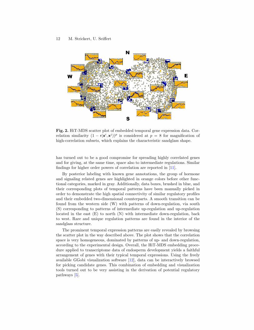
For the 4824 genes of interest, HiT-MDS embedding requires only 100 data cy-cles, processed within a few minutes, to get the high-quality display shown inFigure 2. The characteristic sandglass shape results from using eighth power ofthe correlation measure, (1− r(xi, xj))8. This power magnifies subtle dissimilar-ities in highly correlated genes which leads to focus on a good reconstruction– and thus a fair differentiation – of highly correlated, i.e. with near zero dis-similarities, rather than of obviously discorrelated genes. The exponent of eight


Fig. 2. HiT-MDS scatter plot of embedded temporal gene expression data. Cor-relation similarity (1 − r(xi, xj))p is considered at p = 8 for magnification ofhigh-correlation subsets, which explains the characteristic sandglass shape.

has turned out to be a good compromise for spreading highly correlated genesand for giving, at the same time, space also to intermediate regulations. Similarfindings for higher order powers of correlation are reported in [11].

By posterior labeling with known gene annotations, the group of hormoneand signaling related genes are highlighted in orange colors before other func-tional categories, marked in gray. Additionally, data boxes, brushed in blue, andtheir corresponding plots of temporal patterns have been manually picked inorder to demonstrate the high spatial connectivity of similar regulatory profilesand their embedded two-dimensional counterparts. A smooth transition can befound from the western side (W) with patterns of down-regulation, via south(S) corresponding to patterns of intermediate up-regulation and up-regulationlocated in the east (E) to north (N) with intermediate down-regulation, backto west. Rare and unique regulation patterns are found in the interior of thesandglass structure.

The prominent temporal expression patterns are easily revealed by browsingthe scatter plot in the way described above. The plot shows that the correlationspace is very homogeneous, dominated by patterns of up- and down-regulation,according to the experimental design. Overall, the HiT-MDS embedding proce-dure applied to transcriptome data of endosperm development yields a faithfularrangement of genes with their typical temporal expressions. Using the freelyavailable GGobi visualization software [12], data can be interactively browsedfor picking candidate genes. This combination of embedding and visualizationtools turned out to be very assisting in the derivation of potential regulatorypathways [5].


4.2 Clustering

Beyond the described visual sub-grouping of embedded gene expression data,dedicated clustering methods provide more reliable clusters. Since these methodsdo usually operate in the original data space and not in the somewhat lossyreconstruction of embedded data, higher quantization accuracy can be obtained.

In a previous study, neural gas has been successfully applied to subdividingthe set of 4824 genes into smaller sets of characteristic regulation patterns [5].In principle, such a partitioning helps to get an abstract view upon the data set,because the data space gets faithfully covered by a pre-defined number of typicalcentroids. Such a relatively small number of centroids helps to identify poten-tial cascades of regulatory events by looking at temporal delays of transcriptionactivity. The benefits over hierarchical clustering are two-fold: firstly, the hier-archical clusters would need to be merged appropriately for data abstraction,requiring an extra step; secondly, with NG-C no decision must be taken aboutthe linkage method – one of complete, single, or average linkage – needed for treecreation in hierarchical clustering. Hierarchical clustering is of interest rather forthe identification of outliers.

Certainly the number of centroids is an interesting choice for NG-C, becauseit defines the level of abstraction. For k-means, which is used for the same purposeas NG-C, a number of heuristic methods exist to give rough estimates about thenumber k of centroids [13]. The pragmatic approach suggested here is to computethe centroids and embed them together with the data. The obtained display willthen give reasonable hints, if all major modes, i.e. high density regions, arecovered by the centroids. If not so, their number has to be further adjusted untila good correspondence of centroids and data is obtained.

Visualization of embedded centroids. Clustering and visualization of the4824 barley endosperm genes introduced above yields scatter plots shown in Fig-ure 3. For comparison with NG-C, Eisen’s implementation of k-means has beentaken as reference model [14]. Both methods make use of Pearson correlation forcreating sets of similar patterns for centroid calculation, but according to thestandards, k-means calculates averages in Euclidean space, whereas NG-C usescorrelation-optimized updates. The exponential NG-C neighborhood influence isrealized as exponential decay from σ = 23 to σ = 0.001, the update rate is setto γ = 0.001. Both methods were trained with 100 data cycles for 23 centroidpositions.

As most fundamental difference, the final states in k-means, correspondingto the right panel of Figure 3, are quite close and dense at the boundaries of theembedded data manifold, while a more homogeneous spreading is observed forNG-C centroids.

Quality of representation. Beyond visualization, another quality criterionhas been derived from 10 independent repetitions of k-means and NG-C clus-tering, starting from random initialization. Analogous to quantization accuracy,we determine the average correlation of centroids to their represented data. Fork-means we obtained, over 10 runs, an average correlation of r = 0.9329±0.0017


k-means NG-C

Fig. 3. Correlation-based clustering and visualization using HiT-MDS. Left: k-means; right: NG-C. Both methods use Pearson correlation similarity for com-puting locations of 23 centroids. NG-C centroids are more faithfully distributedamong the data.

per centroid with an average standard deviation 0.0881± 0.0038. For NG-C theresults are r = 0.9516 ± 0.0001 with standard deviation 0.0573 ± 0.0004. Thus,NG-C provides higher average correlation with much less standard deviation.The low standard deviation underlines a very important feature of NG-C: thehigh reproducibility of final centroids, independent of their initialization. Thisis one major advantage over k-means for which a poor reproducibility is known.Moreover, and contrary to k-means, unused prototypes do not occur in NG-C,because of its built-in neighborhood cooperation.

5 Conclusions

Gradients of Pearson correlation have been introduced for cost function opti-mization frameworks aiming at reliable data representation.

The quality of models can be assessed already during data processing bylooking at the current cost value. Rigorous comparisons to existing methodshave not been carried out in this work. There is one simple reason: it does notmake much sense to compare an unsupervised model, optimized for a certainpurpose to a model not optimized for it. From a different perspective, why shouldan optimization model be judged by another than the optimization criterion?For example, if PCA optimizes directions of maximum variance and HiT-MDSoptimizes maximum correlation between two data spaces, the only reason forchoosing either approach is its practical use.

A very central statement derived from the claim above, apply methods totargets they are designed for, is to make model update consistent with the datasimilarity. Here, derivative properties of Pearson correlation are used for opti-mization which provides a model space that is in good agreement with the dataspace. An introduced toy example has demonstrated the practical value of thisconsideration. The presented NG-C clustering method realizes an update con-


sistent with the Pearson correlation similarity measure which allows to generatehighly reproducible partitions of the data.

Adequate visualization is certainly a very important tool to accompany moststeps of data analysis. Initial screening yields hints if pronounced clustering canbe expected, and it allows a reasonable choice of the number of centroids byembedding them together with the data. In the presented gene expression studyit turned out that the correlation-based data space is rather homogeneous; itmight thus be worth to look for interesting outliers by interactive browsing orby detection of special nodes in trees from hierarchical clustering.

Finally, the presented cost function frameworks focussing on the Pearsoncorrelation measure are general enough to replace correlation by any measure forwhich mathematical derivatives are available. This opens a very wide perspectiveon future approaches for reliable data-driven biomedical analysis.

Availability

C, MATLAB (GNU Octave), and R source code of high-throughput multi-dimensional scaling (HiT-MDS) and supplemental data is online available athttp://hitmds.webhop.net/.C code of neural gas for Pearson correlation (NG-C) is online available athttp://pgrc-16.ipk-gatersleben.de/˜stricker/ng/.

Acknowledgements

This work is supported by BMBF grant FKZ 0313115 (GABI-SEED-II) and bythe Ministry of Culture of Saxony-Anhalt, grant XP3624HP/0606T.

References

1. Hammer, B., Hasenfuss, A.: Relational clustering. In Biehl, M.,Hammer, B., Verleysen, M., Villmann, T., eds.: Similarity-based Clus-tering and its Application to Medicine and Biology. Number 07131in Dagstuhl Seminar Proceedings, Internationales Begegnungs- undForschungszentrum fuer Informatik (IBFI), Schloss Dagstuhl, Germany (2007)<http://drops.dagstuhl.de/opus/volltexte/2007/1118>.

2. Bolboaca, S., Jantschi, L.: Pearson versus Spearman, Kendall’s Tau correlationanalysis on structure-activity relationships of biologic active compounds. LeonardoJournal of Sciences 5 (2006) 179–200

3. Strickert, M., Schleif, F.M., Seiffert, U.: Gradients of pearson correlation for analy-sis of biomedical data. In: Proceedings of the Argentine Symposium on ArtificialIntelligence (ASAI 2007). (To appear.)

4. Strickert, M., Seiffert, U., Sreenivasulu, N., Weschke, W., Villmann, T., Hammer,B.: Generalized relevance LVQ (GRLVQ) with correlation measures for gene ex-pression data. Neurocomputing 69 (2006) 651–659

5. Strickert, M., Sreenivasulu, N., Usadel, B., Seiffert, U.: Correlation-maximizingsurrogate gene space for visual mining of gene expression patterns in developingbarley endosperm tissue. BMC Bioinformatics 8 (2007)

http://hitmds.webhop.net/

http://pgrc-16.ipk-gatersleben.de/stricker/ng/


6. Lee, H.K., Hsu, A.K., Sajdak, J., Qin, J., Pavlidis, P.: Coexpression Analysis ofHuman Genes Across Many Microarray Data Sets. Genome Res. 14 (2004) 1085–1094

7. Martinetz, T., Berkovich, S., Schulten, K.: “Neural-gas” network for vector quan-tization and its application to time-series prediction. IEEE Transactions on NeuralNetworks 4 (1993) 558–569

8. Cottrell, M., Hammer, B., Hasenfuss, A., Villmann, T.: Batch and median neuralgas. Neural Networks 19 (2006) 762–771

9. Strickert, M., Teichmann, S., Sreenivasulu, N., Seiffert, U.: High-ThroughputMulti-Dimensional Scaling (HiT-MDS) for cDNA-array expression data. In Duchet al., W., ed.: Artificial Neural Networks: Biological Inspirations, Part I, LNCS3696, Springer (2005) 625–634

10. Sreenivasulu, N., Radchuk, V., Strickert, M., Miersch, O., Weschke, W., Wobus,U.: Gene expression patterns reveal tissue-specific signaling networks controllingprogrammed cell death and ABA-regulated maturation in developing barley seeds.The Plant Journal 47 (2006) 310–327

11. Zhou, X., Kao, M.C., Wong, W.: Transitive functional annotation by shortest-pathanalysis of gene expression data. PNAS 99 (2002) 12783–12788

12. Buja, A., Swayne, D., Littman, M., Dean, N., Hofmann, H.: Interactive DataVisualization with Multidimensional Scaling. Report, University of Pennsylvania,URL: http://www-stat.wharton.upenn.edu/˜buja/ (2004)

13. Dudoit, S., Fridlyand, J.: A prediction-based resampling method for estimatingthe number of clusters in a dataset. Genome Biology 3 (2002) 36.1–36.21

14. de Hoon, M., Imoto, S., Nolan, J., Miyano, S.: Open source clustering software.Bioinformatics 20 (2004) 1453–1454

correlation-based data representation

Documents