corporate distress and restructuring with macroeconomic ... · of corporate restructuring as...
TRANSCRIPT

Research Institute of Industrial Economics P.O. Box 55665
SE-102 15 Stockholm, [email protected]
IFN Working Paper No. 780, 2008 Corporate Distress and Restructuring with Macroeconomic Fluctuations: The Cases of GM and Ford
Lars Oxelheim and Clas Wihlborg
1
Forthcoming in Journal of Applied Finance
Corporate Distress and Restructuring with Macroeconomic Fluctuations:
The Cases of GM and Ford
Lars Oxelheim is a Professor of International Business and Finance at the Lund Institute of
Economic Research, Lund University, P.O. Box 7080, SE-220 07 Lund, Sweden, e-mail:
[email protected] and at the Research Institute of Industrial Economics (IFN), P.O. Box
55665, SE-102 15 Stockholm, Sweden, e-mail: [email protected]
and
Clas Wihlborg is a Professor of International Business at the Argyros School of Business and
Economics at the Chapman University, Orange, CA 92866, USA, e-mail:
August 2011
Abstract
Although macroeconomic factors are part of several models for evaluation of credit risk, there is
little effort to distinguish between effects of such factors and “intrinsic” factors on changes in
credit risk. We argue that lenders, management, courts and traders in distressed securities would
benefit from information about the degree to which macroeconomic factors affect changes in the
likelihood of default in order to determine an effective approach to resolving a distress situation.
A model for decomposing changes in default predictions into macroeconomic and intrinsic
factors is presented. The decomposition is firm-specific in order to capture the differential impact
of the macro environment on firms. The model is applied to z-scores of GM and Ford during the
period 1996-2008.The macro-economy has affected the two firms in different ways with
implications for managements’ and creditors’ approaches to restoring their financial health.
JEL Classifications: G11, G32, G33, G34, L16, L62
Key words: credit risk, creditworthiness, Z-scores, default predictions, GM, Ford, restructuring
2
Corporate Distress and Restructuring with Macroeconomic Fluctuations:
The Cases of GM and Ford
Banking crises in a number of countries during the 1990s triggered research on the role of the
macroeconomic environment in corporate defaults. Most models for predicting bankruptcy use a
set of firm-specific variables to predict bankruptcy or probability of default within a certain time
horizon. Recently, a number of models employ macroeconomic factors as well.1
The most well-known and widely used model for predicting bankruptcy or probability of
default within a certain time period is Altman’s Z-score model (Altman, 1968). This and other
default prediction models reviewed below employ market and accounting factors that themselves
depend on macroeconomic conditions along with firm and, sometimes, industry specific
conditions.2 The Z-score model exists in a number of versions to allow predictions for firms with
limited availability of market data and a recent version employs macroeconomic factors as
described in Altman and Rijken (2011).
Whether or not a default probability estimate depends on explicitly recognized
macroeconomic factors, there is potential value for management, creditors and traders in
distressed securities to dig deeper into the role of the macro-economy by analyzing the
contribution of macroeconomic factors to changes in firm-specific predicitive factors. Thereby, it
should be possible to determine whether an increase in the probability of default is caused by
macroeconomic factors or “intrinsic” factors. By “intrinsic” we mean that the factors reflect
firms’ inherent competitiveness based on firm- and industry specific conditions. We argue that
distress caused by a decline in macroeconomic conditions does not usually require the same kind
of corporate restructuring as distress caused by intrinsic factors. The latter factors are under
management control to a greater extent than macroeconomic factors and they are less likely to be
1 See, e.g., Jonsson and Friden (1996), Chava and Jarrow (2004), Duffie et al (2005), Altman, Brady, Resti and
Sironi (2005). These papers present evidence of a negative correlation between the business cycle and default rates,
as well as between the business cycle and loss given default. 2 See e.g. Crouhy, Galai and Mark (2000) for a review of models. See also Allen and Saunders (2004) for a review
of models of systemic effects on credit risk.
3
mean-reverting. Macroeconomic factors are mostly mean-reverting as sources of fluctuations in
aggregate economic conditions.3
One difficulty in using macroeconomic factors for predictive purposes in default
prediction models is that firms differ greatly in their sensitivities to macroeconomic events both
in terms of type of events they are sensitive to, and in terms of strength. Thus, relevant
macroeconomic factors as well as their weights are likely to vary from firm to firm in the same
way risk exposures to, for example, exchange rates and interest rates vary across firms.
In this paper we take Altman’s commonly used Z-score default prediction model and ask
whether and how the scores produced by the model for a particular firm can be decomposed into
components explained by macroeconomic factors, and components capturing intrinsic factors.
The objective of the decomposition is to provide information about the relative weights of
macro-economic and intrinsic factors in the default prediction. This knowledge could affect the
strategy for dealing with a distress situation by restructuring of assets, liabilities or management
change, as well as the valuation of distressed securities on exchanges.
The decomposition we suggest employs observable price variables as indicators of
macroeconomic conditions. Quantity variables on the macro level are excluded if possible
because there is a longer lag before GDP and similar variables can be observed. Changes in price
variables like interest rates and exchange rates are easily observed without a long lag relative to
macroeconomic events. The price variables signal or reveal information quickly about
underlying disturbances. Time is likely to be essential for management and creditors facing
important restructuring decisions when a firm’s survival is at stake.
In the empirical analysis we use a method for decomposition based on the MUST
(Macroeconomic Uncertainty Strategy) analysis in Oxelheim and Wihlborg (2008). This analysis
is a tool for assessing a firm’s intrinsic competitiveness and macroeconomic exposures. The
decomposition is here applied on the Z-scores for GM and Ford for the period 1996-2008.
The remainder of the paper is organized as follows. In Section I we discuss how
macroeconomic and intrinsic factors affect near-term relative to long-term default probabilities
3 Aggregate factors influencing, for example, long term economic growth are obviously not mean-reverting. We are
primarily concerned with sources of macroeconomic fluctuations, however.
4
to different degrees and implications for approaches to distress resolution. Section II contains a
review of different types of models for forecasting default and the role of macroeconomic factors
in these models. The approach to decomposition of changes in credit risk into macroeconomic
and intrinsic components is discussed in Section III. The case studies of GM’s and Ford’s Z-
scores are presented in Section IV. Conclusion follows in Section V.
I. Macroeconomic Factors in Distress Prediction and Resolution
Any proxy for the default probability of a firm (DP) must refer to a certain time horizon. In
general this horizon is relatively short. Over a time horizon up to a year it makes little difference
for the accuracy of the DP whether a firm’s potential distress is caused by intrinsic factors
reflecting the long run competitiveness of the firm or by macroeconomic factors. However,
changes in DP estimates over a period may be used to assess the longer term need for
restructuring and reorganization of the firm. Management and creditors may not want to respond
the same way to an increase in the likelihood of default over a 12 month horizon caused
primarily by mean-reverting macroeconomic conditions, as to an increase in the likelihood of
default caused by a non-competitive product line, poor management or other “intrinsic” factors.
To illustrate the distinction between macroeconomic and intrinsic factors we define DP as
a proxy for default probability over a certain time horizon and show that the information in DP
about the likelihood of default over a longer time horizon depends on the degree of mean
reversion of factors affecting DP. First, the proxy, DP, is expressed as a function of the value of
the firm’s assets, A, and the debt to asset ratio, L:
DP=f(A, L)+, (1)
The error term, , can be interpreted as a measurement error. We express the value of assets as a
sum of the value of intrinsic factors, I, and macroeconomic factors, M:
A=I+M (2)
5
The intrinsic value reflects the long run competitiveness and viability of operations and
depends on, for example, strategy, operational efficiency, know-how, product development, and
management’s ability to deploy and develop resources. Any shift in I as result of managerial
decisions and changes in the competitive environment can be considered permanent i.e. non
mean reverting.
E[It+1]=E[It]+wt+1 (3)
The discount factor is set to zero and w is a shift variable without mean reversion. The
macroeconomic contribution to value, M, can be expressed as
Mt=Mt-1+vt, (4)
where <1 and v is a shift variable with expected value zero. Macroeconomic factors are not
subject to control by management and they are mean-reverting. Any change in M caused by a
shift in v evaporates over time. This assumption is consistent with observations of mean
reversion in stock markets.
Inserting (2), (3) and (4) in (1) we obtain that
DPt = f((It-1+wt + Mt-1+vt); L)+ t (5)
The observed change in DP in any period relative to the previous period is
DPt = f((wt+vt+(1-)Mt-1); L)+t (6)
This expression states that an observed change in the proxy for default probability may
have been caused by an unanticipated shift in the intrinsic factor, w, a shift in the unanticipated
component of the macro-factor, v, a change in the observation error, an anticipated change as a
result of shifts in macroeconomic factors in earlier periods, and a change in leverage.
It follows from (6) that the expected change of DP over the next period depends only on
the mean reversion of macroeconomic factor and the expected change in leverage. Thus, the
effect of a change in DP, DPt, on any future DPt+i declines with the time horizon i if DPt is
caused primarily by macroeconomic factors.
6
In most default prediction models the proxy DP is based on market and accounting data
for a firm and these data reflect both intrinsic and macroeconomic influences on asset value, as
well as leverage. Observation errors () also affect the observed DP relative to the actual default
probability. Even if an observed DP based on market and accounting date captures default
probability with reasonable accuracy over the near term the long run implications depend on the
source of the observed change. To the extent an observed change in DP depends on
macroeconomic factors, a reversion can be expected over the longer term.
In Section III we will decompose observed changes in a proxy for DP into intrinsic and
macroeconomic components. Any change in DP can be considered a signal to management, as
well as to shareholders and creditors, that action is necessary. The appropriate action may depend
on the cause of the change in DP, however.
In the following we discuss how information about intrinsic and macroeconomic sources of
change in the default probability in combination with leverage can be used by management,
shareholders, creditors or courts to assess different types of restructuring procedures in response
to distress. Valuation of distressed securities would depend on the weight of macroeconomic
factors in the prediction as well as the approach taken to resolve distress. We consider the
following types of restructuring procedures:
- Bankruptcy with liquidation of assets as under Chapter 7 in the US Bankruptcy Code.
- Bankruptcy under rehabilitation procedures such as Chapter 11 in the US Bankruptcy Code and
informal work-outs.
- Change of management through hostile takeover, shareholder or board action
- Substantial asset restructuring involving, for example, sale of assets, reorientation of strategy,
partial closing of operations, etc.
- Liability restructuring involving substantial changes in capital structure including reduced
dividend pay-out, debt rescheduling and debt forgiveness.
7
A. Bankruptcy with Liquidation
Bankruptcy occurs when the present value of the cash flows generated by a firm’s assets is less
than the value of the firm’s debt. As long as the present value of the cash flows from the assets is
greater than their scrap value, assets in place have value. If the assets in place have positive value
but the value of debt exceeds the asset value it is common to talk about “financial distress.”
Piecemeal liquidation would lead to an economic loss in this situation.4 Liquidation of the firm
as going concern may be efficient, however, if change in ownership and management could
increase the value of the assets.
If the present value of the cash flows generated by the assets is less than their scrap value
the firm is in “economic distress.” Even the debt-free firm is insolvent in this situation. Assets in
place have a negative value. Thus, piecemeal liquidation is the appropriate course of action and
ongoing operations should be shut down.
Creditors in a leveraged firm would like to avoid financial as well as economic distress
but as soon as insolvency is a fact shareholders with limited liability do not have incentives to
avoid a further deterioration of the firm’s situation. As a result, it may lie in the interest of
creditors to force a firm into bankruptcy with liquidation already in financial distress.
Liquidation does not preclude that assets in place are sold in such a way that ongoing operations
can continue. Bankruptcy procedures including cash auctions make it possible for the whole
business or viable parts of it to be sold to new owners who can deploy and manage the assets
better than current owners.5
Liquidation is clearly an appropriate response to insolvency if the firm is in economic
distress. Even in financial distress liquidation may be appropriate if the distress is caused
primarily by intrinsic factors and current owners are considered unable to redeploy and manage
assets more productively. In this case the liquidation would enable new owners to take over
operations fully and partially.
4 See, e.g., Wihlborg et al (2001)
5 See Thorburn (2006), pp. 155-172. Evidence is presented that in a system without Chapter 11 type law 75% of all
liquidations end up as sales of “going concerns”. Thus the firms continue under different ownership.

8
If insolvency is caused by macroeconomic factors to a substantial extent it is less likely
that management can be blamed for the insolvency. Liquidation can lead to value destruction if
assets in place under current management generate greater value than the scrap value.
Furthermore, the value of the firm is likely to increase once there is a macroeconomic
turnaround. In this situation the restructuring of the following type should be considered.
B. Bankruptcy under Rehabilitation Procedures and Informal Work-outs
Chapter 11 in the US allows the incumbent management and current owners to retain control of
an insolvent firm. Once in Chapter 11 management negotiates with creditors for debt relief,
rescheduling of loans and possibly some asset redeployment or sale. As noted above, such a deal
can be economically efficient under financial distress, if the current management team is
considered qualified. In particular, if current asset values can be expected to recover, a focus on
restructuring of liabilities in the short run can be economically efficient. In other words, the
greater the weight of macroeconomic conditions in insolvency, the stronger is the case for a
focus on liability restructuring under rehabilitation procedures. Clearly, current owners and
management must have incentives to manage assets in the most efficient manner. Such
incentives could be restored by, for example, debt relief that lifts the value of equity above zero.
The implication of this discussion is that Chapter 11 procedures are appropriate if management
performs well, asset in place have positive value and macroeconomic conditions have
contributed strongly to the distress.
Many countries do not have easily accessible rehabilitation procedures of the Chapter 11
type that allows current owners and management to retain control and re-emerge from
bankruptcy.6 The incentives for owners and management to negotiate informal work-outs with
creditors are strong in countries lacking Chapter 11 type of rehabilitation procedures. Creditors
also have an incentive to contribute to informal work-outs if the firm’s intrinsic value is likely to
remain positive if the level of debt can be reduced. Thus, if macroeconomic factors have
contributed strongly to insolvency, creditors as well as shareholders have incentives to negotiate
temporary debt relief by means of bridge loans or rescheduling. If the insolvency is caused
6 See Wihlborg et al (2001)
9
primarily by intrinsic factors, creditors could support debt relief up to a point where the intrinsic
value of the firm’s assets exceeds the debt provided creditors have faith in the management team.
Under Chapter 11 the incentives to seek bankruptcy protection can be strong even if
intrinsic factors are the major cause of distress since commitments to labor or other stakeholders
with claims can be renegotiated. In this case it lies in the interest of the court to determine
whether distress is caused primarily by macroeconomic factors or whether the firm is trying to
avoid consequences of prior commitments or liability for damages it has caused.
C. Change of Management
As noted, Chapter 11 is most suitable for situations when creditors have faith in the owners and
managers of a distressed firm. An increased probability of default caused by macroeconomic
factors can be blamed on management only under specific circumstances. Specifically, a highly
leveraged firm is likely to be relatively sensitive to macroeconomic conditions. Even so, the
benefits of changing management in response to an increased probability of default caused
primarily by macroeconomic events are not likely to be large. On the other hand, an increased
probability caused by intrinsic factors can be interpreted as a signal that assets are deployed
poorly or that strategies are not executed well. In this case shareholders as well as creditors
would want to change management. Management can be entrenched, however, with the result
that only a takeover makes a change in management possible. In cases when a takeover is not
feasible, bankruptcy is the last opportunity to change management.
D. Substantial Asset Restructuring
A takeover usually implies that the incumbent management team is ousted. Thus, the team has an
incentive to do what is necessary to avoid that the firm becomes a takeover target. In accordance
with the discussion above, observation of an increasing default probability caused by intrinsic
factors can be seen as a signal to management that substantial asset restructuring is necessary.
This restructuring can be more or less far-reaching depending on level and rate of change of the
default probability.
10
E. Liability Restructuring.
Any increase in the default probability should always be taken seriously and management can
never be complacent with respect to the deployment of assets. However, if the increase is caused
by macroeconomic factors and it reaches an uncomfortable level it should be taken as a signal
that the capital structure of the firm is inappropriate in the macroeconomic environment. Either
leverage should be reduced or macroeconomic risk management needs to be strengthened.
In summary, a increase in the near term default probability, DP, caused by
macroeconomic factors can be viewed as relatively good news for management since it cannot be
blamed for this increase and the change in the observed DP is likely to be reversed. If intrinsic
factors dominate the increase in the near term DP, shareholders and creditors need mechanisms
for removing management. A takeover is one such mechanism prior to insolvency. Once
insolvency occurs liquidation under bankruptcy would become the relevant instrument.
Bankruptcy under Chapter 11 would be appropriate if the insolvency is caused primarily by
macroeconomic factors and assets in place have a positive value.
Valuation of distressed securities on exchanges can provide valuable signals about the
expectations of market participants with respect to asset values, management quality and the
contribution of macroeconomic factors to the extent there are market participants with ability to
separate the impact of macroeconomic factors from intrinsic factors.
II. Predicting Corporate Default in the Literature
In this section, different type of credit scoring models will be discussed from the perspective of
their intent and capacity to recognize the influence of macroeconomic factors in the estimation of
credit risk.
A. Altman's Original Z-score Model
From a wide range of book and market value ratios, Altman (1968) used Multiple Discriminant
Analysis to identify the following model for predicting bankruptcy in the USA:
11
Z-score = .012X1 + .014X2 + .033X3 + .006X4 + .999X5 (7)
where X1 = Working capital / Total assets
X2 = Retained Earnings / Total assets
X3 = Earnings before interest and taxes / Total assets
X4 = Market value of equity / Book value of total liabilities
X5 = Sales / Total assets
Z = Overall index
In this model the first four firm-specific values on the right-hand side are given as
percentages (or multiplied by 100 if given as absolute values) whereas the final value is given as
an absolute (number of times). For example if the X1-value is 10% the number 10 is used in the
model.7 From his original sample of 66 firms (of which 33 did go bankrupt) Altman observed
that, in general, firms with a Z-score greater than 2.99 did not go bankrupt and firms with a Z-
score below 1.81 went bankrupt within a year. Firms with Z-scores in between were in the “grey
area”.
There is no independent role of macroeconomic variables in the original Z-score model.
The variables constituting the score are affected by firm- and industry specific, as well as
macroeconomic conditions. Thus, the contribution of intrinsic versus macroeconomic factors to a
low Z-score cannot be observed directly.
Over the years Altman has presented modified versions of the Z-score. The Z’- score for
non-traded firms substitutes book values for market values in the X4-factor. Another version, the
Z’’-score model, does not include the X5-variable. This model should be used for analyzing
emerging market firms and for non-manufacturers as well as for manufacturers. The classic Z-
score model is mainly applicable to manufacturers, such as GM and Ford. In the most recent
version of the model Altman includes macroeconomic factors as well to estimate the “Z-metrics
7 See Altman (2000), personal homepage for more about the Z-score model.
12
Scores” and DPs of individual firms. This model is proprietary, however, (see Altman et al, 2010
and Altman and Rijken, 2011). We did obtain relevant estimates for GM and Ford from this
model, see Section IV below.
Altman and Hotchkiss (2005) translate Z-scores into probabilities of default over a
specific time horizon by analyzing the relationship between Z-scores and default probabilities
(mortality rates) for corporate bonds over their lifetime. The Z-metric scores are similarly
translated into probabilities over different time horizons. Altman and Rijken (2011) show that the
proprietary Z-metrics model performs better in terms of Type 1 and Type 2 errors for default
probabilities. Given the restriction implied by the proprietary we here employ the original, non-
proprietary Z-score model and take the Z-scores as bankruptcy indicators in the empirical
analysis below. Altman (2002, 2006) and Das et al (2009) show that the model has performed
well for American firms on a one-year horizon and that it has outperformed the KMV model (see
below) during recent years.
B. Bankruptcy Prediction Incorporating Macroeconomic Variables
As noted Altman’s Z-metrics model adds macroeconomic variables to the original Z-score
model. Carling et al (2007) introduce macroeconomic factors along with accounting data,
payment behaviour, and loan related conditions in a model of default risk for Swedish firms.
This very data-intensive model explains the survival time to default for business borrowers in the
loan portfolio of a Swedish bank that provided the data. By introducing macroeconomic factors
the authors improve on predictions of the absolute level of the probability of default, while
models without macroeconomic factors are reasonably accurate only with respect to rankings of
default risk. The significant macroeconomic factors are the output gap, the yield curve and
Swedish households’ expectations about the economy.
Jacobson et al (2008) use a very large panel data set including all Swedish corporations
(limited liability businesses) during a 12 year period to analyze factors that explain defaults and
to derive probabilities of default conditional on firm specific, industry and macro factors. The
authors compare out of sample predictions with and without macro factors. These factors are the
same as those used in Carling et al (2007). The results indicate that default risk estimates are
13
improved by the inclusion of macroeconomic factors. Another result is that predictions are
improved by estimating the model on the industry level rather than the aggregate level.
The macroeconomic factors employed in these models are useful for the analysis of
historical default data although the output gap and similar variables are observed only with a lag.
As noted, this observation lag is a disadvantage for the internal or external analyst whose
objective it is to determine whether changes in the probability of default depend on intrinsic or
macroeconomic conditions.
C. Bankruptcy Prediction Based on Option Pricing Theory
Bankruptcy prediction based on option pricing theory was introduced by Robert Merton (1974).
Using insights gained from the development of the option pricing model developed by Black and
Scholes (1973) and Merton (1973), he described the payoff from a default-risky bond in terms of
the pay-offs on a risk-free bond and a put option on the value of the firm’s assets. The borrower
holds a put option and its value depends on the value of the firm’s assets, the face amount of
debt, the volatility of the asset value, the time to maturity of the bond, and the yield on a default-
free bond with the same time to maturity. The difference in yield between the default-risky and
the default-free bond is the credit spread. This spread is a put option premium that increases with
leverage and asset value volatility.
The KMV model puts the Merton model to practical use as described in Vasicek (1997)
and Kealhofer (1995, 1998). KMV Corporation (now owned by Moody’s) is a company
specializing in credit risk analysis. The model uses an Expected Default Frequency (EDF), which
is firm specific and a function of the capital structure of the firm, the volatility in the returns of
assets and the current asset value. The first step in estimating the EDF is estimating the asset
value and the volatility of the asset returns. If all liabilities of the firm were publicly traded, it
would be a rather simple task to estimate the asset value. As this is not ordinarily the case,
however, the value of the liabilities is estimated using the Merton approach. The second step is
estimating the distance-to-default, which is defined as the number of standard deviations
between the mean of the probability distribution of the future asset value and the so called
default point, defined as the sum of the short-term debt and half the long-term debt. The third
14
and last step is relating the distance-to-default statistic to historical data on default frequencies of
firms with different distances-to-default. Thereby, a probability of default for a firm is estimated.
Like the Z-statistic, the EDF statistic depends on firm-, industry- and macroeconomic
factors. Thus, the contribution of macroeconomic factors could in principle be analyzed by
estimating the contribution of macroeconomic factors to volatility and asset values.
D’Amato and Luisi (2006) and Tang and Yan (2010) examine how aggregate output and
inflation affect the term structure of credit spreads. The first-mentioned authors estimate the
contribution of macro factors to EDF’s by assuming that that they are determined by the same set
of indicators of real and financial activity as credit spreads. They analyze how spreads depend on
the factors and apply the results on EDFs. Under these assumptions macroeconomic indicators
have significant predictive power for future default risk. Dufresne et al (2001) also explain credit
spreads incorporating macroeconomic variables.
Pesaran et al (2005) link a global macroeconomic model to a credit risk model of the type
described. They use equity indices, interest rates, inflation, real money balances, output and oil-
prices to explain changes in credit risk across industries and firms. Pesaran et al (2006) extend
the model to consider diversification of credit risk. Opportunities for diversification depend on
the importance of macroeconomic factors.
The Credit Metrics model developed at JP Morgan (1997) builds on the models described
but introduces the credit migration approach as well. It includes the risk of default of a company
with a specific credit rating. Essential to the model is also the transition matrix stating
probabilities of changes in ratings conditional on current ratings. These probabilities are derived
from historical data. Macroeconomic factors can be introduced in the analysis as in the KMV
model above.
15
D. An Actuarial Approach
CreditRisk+8 is a model used by Credit Suisse. It focuses solely on the default risk, not the risk
of credit downgrading. Probabilities are obtained using historical data. Within a portfolio of
bonds the number of defaults per period is assumed to follow a Poisson distribution.
The main advantage of the model is that it is simple to use. There is no explicit
consideration of macroeconomic fluctuations influencing probabilities of default over time,
however.
E. Industry and Macroeconomic Models of Default Probabilities
A few default prediction models rely entirely on industry-and macro variables. For example,
CreditPortfolioView is a risk assessment model developed in Wilson (1997a and b) and adopted
by McKinsey. It relates the default probability for a firm in an industry to changes in country-and
industry-specific variables. The model assumes that the default probability follows a logit
distribution:
Pj,t = 1 / (1 + e-Yj,t
) (8)
Where Pj,t is the probability of default in country/industry j in period t, and Yj,t is an index value
from a multi-factor model wherein country- and industry-specific factors are introduced. Using
logit estimation, coefficients expressing the contribution of each factor to the probability of
default within an industry can be estimated. Since the analysis is performed on the industry level
it is assumed that firms within an industry are homogeneous with respect to impact of
macroeconomic variables.
III. Decomposing Z-values into Intrinsic and Macroeconomic Components
Most of the default prediction models discussed so far use firm specific accounting and market
variables or a combination of firm-specific and macroeconomic variables. The former variables
are likely to depend on macroeconomic condition. Therefore, it is necessary to identify how the
firm-specific variables depend on macroeconomic conditions in order to decompose default
predictions into intrinsic and macroeconomic components.
8 See Credit Suisse, (1997)
16
To illustrate our approach to decomposition into intrinsic and macroeconomic factors we
use Altman’s original Z-score model to obtain proxies for the default probabilities for firms. The
same approach can be used to decompose other proxies.
The choice of macroeconomic variables in the decomposition of default predictions is
based on two criteria. First, they should reflect the macroeconomic impact on a firm’s default
probability as well as possible. Second, they should be observable as quickly as possible after a
macroeconomic event. Speed is of essence for management, creditors and traders in distressed
securities to act on the information about sources of change in default predictions.
The first criterion implies that it may be necessary to use a different set of macro
variables for different firms. The analyst needs to identify the specific macroeconomic factors
that affect a particular firm’s default probability, as well as the strength of each factor, in order to
gain information about the appropriate restructuring strategy in an approaching or actual distress
situation.
We follow the MUST-approach - developed by Oxelheim and Wihlborg (2008) in a
Value Based Management (VBM) context - for decomposing credit scores or estimated default
probabilities into macroeconomic and “intrinsic” components based on frequently observable
variables. Following this approach a set of macroeconomic variables of potential relevance for a
firm is identified before the relevant variables are identified econometrically. The approach
focuses on price variables as indicators of the impact of the macro-economy because price
variables are observed without much lag. According to economic theory changes in prices reflect
underlying disturbances under certain assumptions about, for example, price flexibility. If these
assumptions are not satisfied it is possible that both price and quantity variables are required to
capture macroeconomic conditions fully.9 We return to these issues in the case discussion in
Section IV.
To observe the sensitivity of a firm’s default probability to macroeconomic variables we
decompose the Z-score into two parts following the discussion in Section I:
9 The price variables are stable indicators of effects of macroeconomic conditions on a firm level indicator if there is
a systematic relationship between a shock of a particular type and its effects on the firm level indicator and a group
of price variables.
17
Zi,t = ZI,i,t + ZM,i,t (9)
In the above expression Zi,t is the total Z-score of company i at time t according to Altman’s Z-
score model, ZI,i,t is the intrinsic part of the Z-score of company i at time t and ZM,i,t is the part of
the Z-score that depends on macroeconomic fluctuations. Thus, Z, ZI and ZM correspond to DP, I
and M, respectively, in expressions (2)-(6). The Z-score also includes factors capturing leverage,
L, in Section I. The Z-score model can be expressed in the following way:
ZI,i,t + ZM,i,t = .012 X1,i,t + .014 X2,i,t + .033 X3,i,t + .006 X4,i,t + .999 X5,i,t (10)
where X1 - X5 are defined as in Equation (7).
We expect that each of the Z-score factors, X1,i,t through X5,i,t, is sensitive to
macroeconomic fluctuations. Each of them can be decomposed into an intrinsic and a
macroeconomic component:
Xi,t = XI,i,t + XM,i,t (11)
where Xi,t stands for one of the X variables above for firm i in period t. XI,i,t is the intrinsic
component of this variable and XM,i,t is the macroeconomic component. The new Z-score model
with factors that depend on changes in macroeconomic variables is:
Zt = ZI,t + ZM,t = .012 (XI,1,t + XM,1,t) + .014 (XI,2,t + XM,2,t) + .033 (XI,3,t + XM,3,t) +
.006 (XI,4,t + XM,4,t) + .999 (XI,5,t + XM,5,t) (12)
As expression (12) shows there are two ways to decompose a firm’s Z-score. Either the
decomposition can be performed on the total Z-score after X1 through X5 have been added
together or each of the factors X1-X5 can be decomposed separately into intrinsic and
macroeconomic components and, thereafter added to obtain ZI and ZM in each period. We choose
the former approach and decompose Zt directly without decomposing each factor X1-X5. The two
approaches should be equivalent if the macroeconomic contributions to the different components
of the Z-score remain constant over time in relative terms. Even if the relationship between each
component and macroeconomic factors are unstable over time, this alternative approach should
be more robust since the relationship between the total Z-score and macroeconomic factors is
18
likely to be more stable than the component relationships. The reason is that the impact of the
macro economy can shift among the component variables over time.
As mentioned, the focus in the MUST-approach is on macroeconomic price variables; i.e
on exchange rates, interest rates and inflation rates. The extent to which changes in Z in a period
depends on changes in macroeconomic factors can then be expressed in the following way:
dZM,i,t = ((ZM,i)/(e)) • det +((ZM,i)/(i)) •dit + ((ZM,i)/(p))•dpt (13)
In this expression det, dit, and dpt represent changes in sets of exchange rates, interest
rates and price levels during a period. The partial derivatives show the sensitivity of the Z-score
to changes in the macroeconomic factors. A particular firm may very well be affected by
domestic as well as several foreign macroeconomic factors with different sensitivities.
Econometrically, the macroeconomic influences on the Z-scores are identified in
regressions with changes in Z-scores as the dependent variables and macroeconomic as well as
industry and firm-specific variables as independent variables in order to account for possible
correlation between macro economic factors and factors that affect firms’ intrinsic credit risk.
In the next section we use Z-scores for GM and Ford to illustrate how the relevant
macroeconomic price variables are identified, and how changes in Z-scores are decomposed
period by period.
IV. Decomposition of Z-score Changes for GM and Ford; Restructuring and Survival?
In this section we begin by calculating the quarterly Z-scores for GM and Ford for the period
1996 (1st quarter) - 2008 (3
rd quarter). Thereafter, we regress changes in Z-scores on
macroeconomic and industry price variables. The estimated coefficients for the macroeconomic
variables are used to decompose the changes in Z-scores into changes caused by macroeconomic
factors and by intrinsic factors. The decomposition should allow us to observe how
macroeconomic factors have affected default probabilities for the two companies relative to
intrinsic factors during the period and their need for more or less fundamental restructuring in
2008
19
The variables that together build up each Z-score were obtained from GM’s and Ford’s
quarterly statements. These variables, defined in Section II, depend individually on
macroeconomic factors but, as mentioned, we choose to decompose the Z-score rather than its
components.
We regress actual Z-scores rather than estimates of corresponding default probabilities
from Altman and Hotchkiss (2005). The Z-scores are the variables that were derived in the
original default prediction model. It is possible that these scores do not translate into the same
probabilities of default for these two firms as for the average firm. GM and Ford are two very
large corporations that can be expected to survive lower values of distress indicators than most
firms as noted in Altman (2002, 2006).
We have been given access to the proprietary estimates of default probabilities based on
the more recent Z-metrics model but these estimates do not go as far back as the Z-scores,
however. Since the number of degrees of freedom is a critical issue we therefore work with the
Z-scores which also can be replicated by other researchers.10
The levels of the quarterly Z-scores are presented in the second column of Tables II for
GM and Table III for Ford. GM’s score has fluctuated between 1.83 and -.95. The score was
actually declining during most of the period as Figure 1 shows. The corresponding figures for
Ford are 1.86 and 0.015. Figure 2 shows also for Ford’s Z-score a trend wise decline over a large
part of the period. The decline was slower, however, and Ford’s Z-score recovered sharply in
2005.
According to Altman’s rule of thumb for his original sample of firms, these low Z-scores
for the whole period for both companies would indicate that the likelihood of bankruptcy within
a year was high during the whole period. Altman (2006) has later concluded that the rule of
thumb stating that bankruptcy is very likely within a year if the score falls below 1.8 does not
apply to very large corporations like GM and Ford. There is no doubt the scores are very low,
however, and that they indicate a high probability of bankruptcy for both corporations
throughout the period.
10
We regressed quarterly averages of daily Z-Metrics on the Z-scores and the log of the Z-scores. The variables are
strongly positively correlated but their patterns are different enough to merit further analysis.
20
The changes in the Z-scores are shown in the third column of Tables II and III11
. These
data are the independent variables in the regressions below. Thereafter we decompose these
changes into intrinsic and macroeconomic factors. The average quarterly change for GM in
Table II is -0.026 with a standard deviation of .37. The corresponding figures for Ford in Table
III are 0.0065 and .31. The variation from quarter to quarter is substantial. For expositional
reasons the data in Figures 1 and 2 are moving averages for three quarters.
Insert Tables I-III here
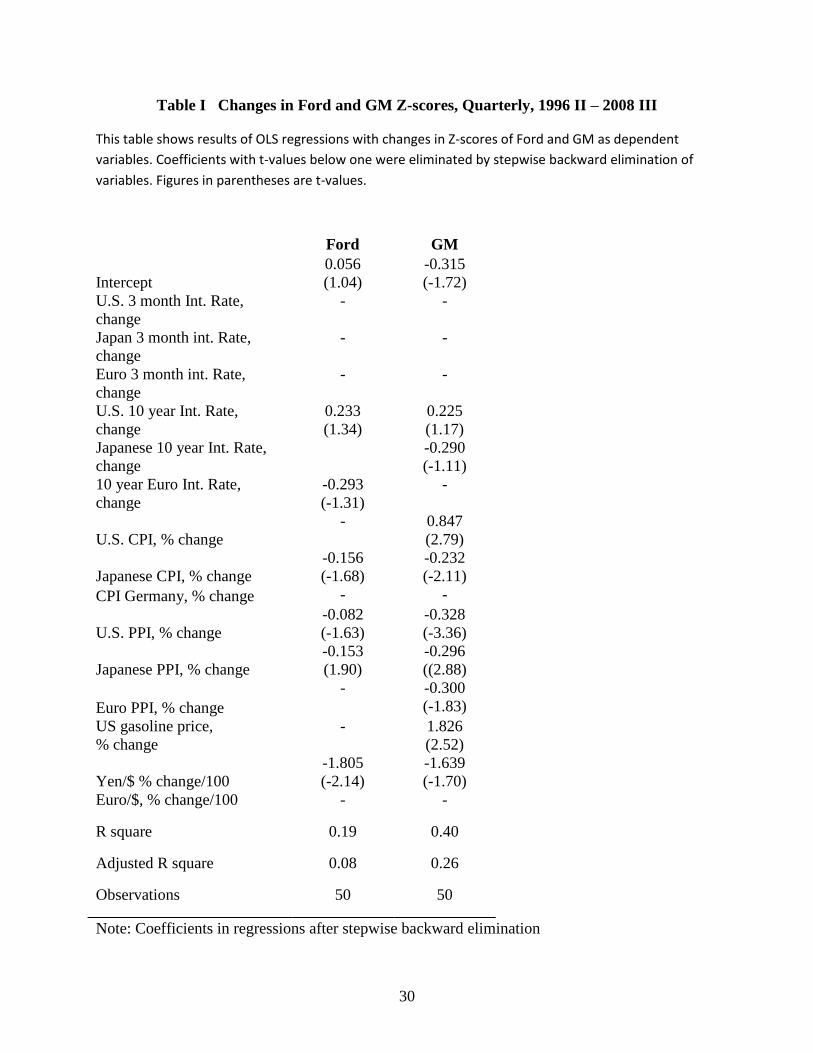
Two regression results for changes in Z-scores for each firm are presented in Table I. The
table includes only results for the final regressions after a step-wise backward elimination
procedure has been carries out. We have chosen to include coefficients at a relatively low level
of significance (t-values greater than one) for the purpose of decomposition.
Before arriving at the results presented in Table I the regressions for Z-score changes
were run with a larger set of potentially relevant variables for each of the two companies. Since
both Ford and GM are worldwide companies in the same sector the macro variables for both
firms included exchange rate changes, long term and short term interest rate changes and
inflation variables in regions which jointly should represent US as well as global developments.
The relevant independent variables were identified in a fundamental analysis of each company as
answers to the following questions: a) where does the company produce? b) which are the
company’s major competitors and where do they produce? c) from where does the company buy
inputs? d) from where do the company’s competitors buy inputs? e) which are the company’s
major geographical markets? and, finally, f) which are the major currencies among the
company’s financial positions? To confirm that price variables are sufficient to capture
macroeconomic conditions we also included GDP growth in the US. Inclusion of this variable
does not increase the explanatory value. Thus, we include only price variables that rapidly reflect
macroeconomic conditions.
In the fundamental analysis of Ford 23 price variables from Europe, Japan and the US
were identified as having a potential economic explanatory value. The fundamental analysis of
11
The changes are differences between two Z-score levels rather than percent changes because the scores are close
to zero and negative values exist.
21
GM resulted in a set of 17 independent variables from the same three regions. Among the
variables are 3-month and 10-year interest rates in the US, Japan and the euro area; the euro/$
and the yen/$ exchange rates, CPI inflation in the US, Japan and the euro area and PPI inflation
in the same three areas. In addition, gasoline price changes in the US were included. Lagged
variables were introduced with little effect on the results.
Both changes in CPI and PPI are included to capture the relative price change between
these variables as well as inflation. This relative price serves as a proxy for the relative price
between manufacturing goods and services. Instead of this relative price we could have included
the relative price for motor vehicles as an industry specific price variable but the two relative
prices are highly correlated.
It can be debated whether the gasoline price should be considered an industry specific
variable or a macro variable. It is certainly a variable beyond management control and it affects
the whole economy but it may be particularly important for car manufacturers.
The dependent variable is the unit change in the Z-score from the previous quarter.
Percent changes cannot be used since there are values close to zero and a few negative
observations. Exchange rate-, price level- and gasoline price changes are measured as percent
rates of change for period averages relative to the previous quarter. Interest rates changes are
measured as percentage point changes. Period averages are used because most of the input
variables in the Z-scores are quarterly flows.
The results of the regressions are presented in Table I. Only a subset of the variables
turns out significant in the two regressions since the correlations among several of the variables
are high. Thus, only a subset of the variables is required to capture most of the macroeconomic
influences on the Z-scores. The relevant macro factors for the two firms turn out to be different.
The variables the two companies have in common are the US 10-year interest rate, CPI-inflation
in Japan, PPI changes in the US and Japan, and the Yen/$ exchange rate. The coefficients for
these variables are quite similar for the two firms. 3-month interest rates and the euro/$ exchange
rate are not significant for any of the companies. Nevertheless, macroeconomic conditions do not
seem to affect the firms in identical ways. There is one variable influencing only Ford’s Z-score
22
(the 10-year euro interest rate) while only GM’s Z-score is influenced by Japan’s 10-year interest
rate, US CPI-inflation, Europe’s PPI inflation and gasoline prices in the US.
The US 10 year interest rate increases the Z-score for both companies while one of the
other 10-year interest rates affect each company’s Z-score negatively. A positive effect
indicating a declining likelihood of default can be explained by the correlation between the
interest rate and the general level of economic activity. It can be observed that an equal increase
in the 10 year interest rates in the three regions has a negative effect on the Z-scores of both
companies. The magnitude of this global interest rate effect captured by the sum of the interest
rate coefficients is nearly the same for the two firms although they are sensitive to different
interest rates. Differences between the two firms are partially accounted for by US CPI-inflation
affecting only GM’s Z-score positively and strongly. Inflation in Japan affects both companies
negatively and to a much smaller degree. PPI inflation (at a constant CPI inflation) has a
negative effect on Z-scores in all cases.
A depreciation of the Yen has approximately equal negative effects on the Z-scores of
both companies. The explanation is most likely that a depreciation of the yen increases the
competitiveness of Japanese car manufacturers.
Another difference between the firms is that an increase in gasoline prices in the US has a
significant and positive effect on the Z-score of GM but no effect on the Z-score of Ford. A
possible explanation for this result is that GM benefited relative to Ford of an increase in
gasoline prices. During a large part of the period Ford’s depended to a greater extent than GM on
relatively gas guzzling SUVs. It is also possible that GM responded more strongly to changes in
gasoline prices with, for example, sales incentives. Sales is a variable with substantial influence
on the Z-scores.
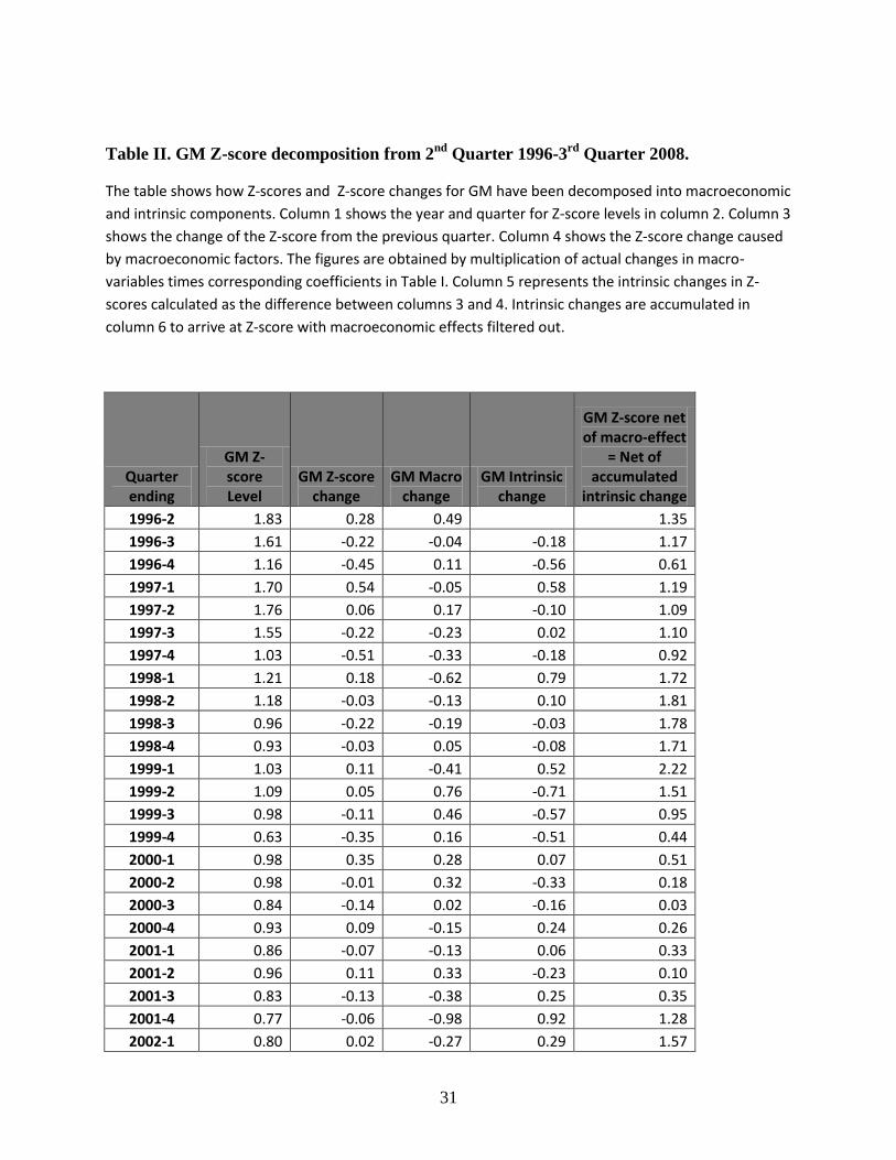
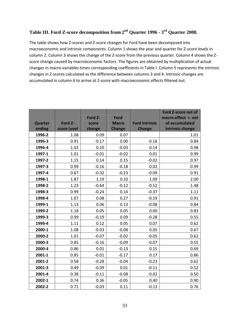
We turn now to the decomposition of the Z-scores and the changes of these scores in
Table II for GM and Table III for Ford. The columns “Macro change” are obtained by
multiplying the regression coefficients in Table I with actual changes in the macroeconomic
variables for each period. The following expression shows how the macro effects have been
calculated for Ford in each period:
Macro change Ford = 0.233 (change 10-year US interest rate)
23
- 0.293 (change in 10-year euro interest .rate)
- (0.156 + 0.153) (Japan CPI inflation-average)
- 0.082 (US CPI inflation-average)
- 0.0181 (% change in Yen/$) (14)
Inflation variables are defined as deviations from the period average in (14) in order to remove
long term trend effects of continuous inflation. Such long term trends should be neutral with
respect to the default probability of the firm.
The coefficients for the CPI inflation terms are the sum of the coefficients for CPI
inflation and PPI inflation in Table I. PPI inflation per se does not appear as a macroeconomic
variable. Thereby we have removed the impact of the relative price change between PPI and CPI
from the regressions.12
This relative price change is considered an intrinsic variable.
The macro effect in a particular period for GM is calculated using the following
expression:
Macro change GM = 0.225 (change 10-year US interest rate)
- 0.290(change in 10-year Japan interest rate)
- (0.232+0.296)(Japan CPI inflation-average)
+ (0.847-0.328)(US CPI inflation-average)
- 0.300(euro CPI inflation-average)
- 0.0183(% change in Yen/$)
+1.826(% change gas) (15)
12
Note that a∆CPI + b∆PPI = (a+b)∆CPI + b(∆PPI-∆CPI). The left hand side of this expression appears in the
regression. The right hand side consists of the inflation effect as shown in expressions (14) and (15) and the relative
price effect which is considered intrinsic.
24
The columns denoted Macro change in Tables II and III are obtained when actual changes in
macro variables each period are inserted in expressions (14) and (15). The next column in the
tables show the intrinsic changes each period calculated as the Z-score change minus the Macro
change.
The mean quarterly macro change for GM is 0.045 and the mean intrinsic change is
negative -0.071. Thus, the macro effect including gasoline price changes have contributed
positively to GM’s Z-score change for the whole period. The corresponding figures for Ford are
0.001 and 0.005. Although the differences between total and intrinsic changes for the whole
period are small, the average macroeffect made GM look better and made Ford look worse than
what was caused by intrinsic changes in default probability. Thus, the average macro effect is
smaller and the average intrinsic change is positive although small. However, the average
changes hide substantial variation in the impact of macro variables as well as in intrinsic changes
in Z-scores.
The final column in the tables shows levels of the Z-scores after removing accumulated
macro effects under the assumption that the macro effect in the first quarter of 1996 was zero.
We may call the figures in these columns the “Intrinsic Z-scores” for the two firms. The numbers
are obtained by removing the accumulated intrinsic changes beginning with the Z-scores in 96
quarter II after removing that quarter’s macro change from the initial Z-score levels.
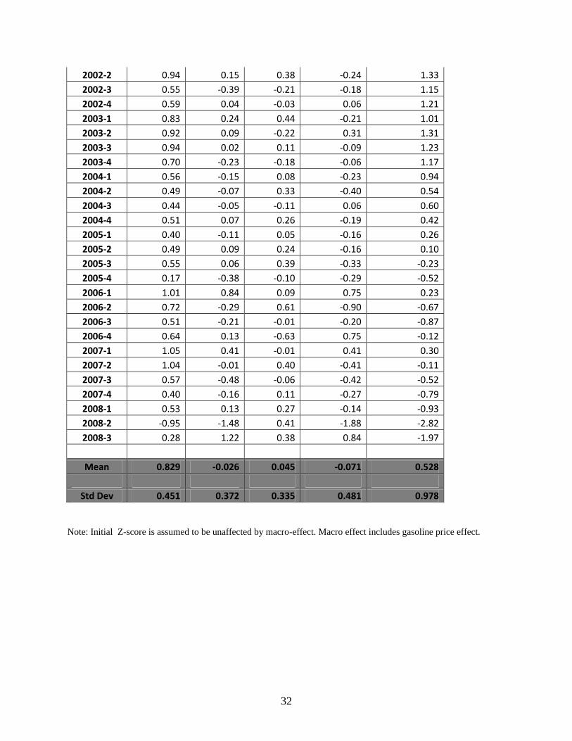
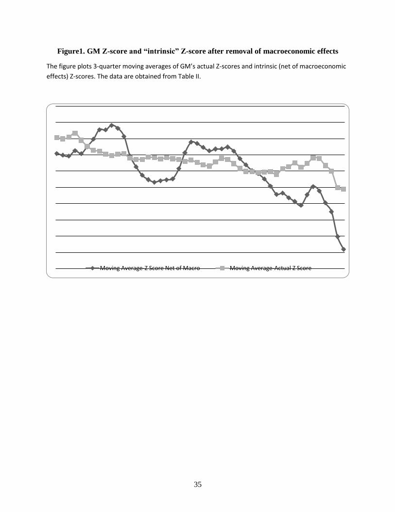
Figure 1 plots three-quarter moving averages of GM’s Z-scores net of accumulated macro
effects. Figure 2 plots the moving averages of Ford’s Z-scores and Ford’s intrinsic Z-scores net
of accumulated macro effects.
Insert Figures 1-2 here
The GM plots show greater impact and greater variation of the impact of the macro
economy on the Z-scores than on the Ford plot. In Figure 1 the “Intrinsic Z-score” fluctuated
around the actual Z-score until mid 2004. Thereafter, were it not for the macroeffect GM’s Z-
score would have been falling almost continuously until the end of the data period in the third
quarter of 2008. The macro effect even contributed to a slight increase in GM’s Z-score from
2004 through 2006. Through 2007 and 2008 both the actual and the “intrinsic” Z-score fell
dramatically. The latter even became negative. Thus, the macro-effect obscured the steep decline
25
in GM’s intrinsic ability to survive. This intrinsic decline was almost continuous beginning in
2003.
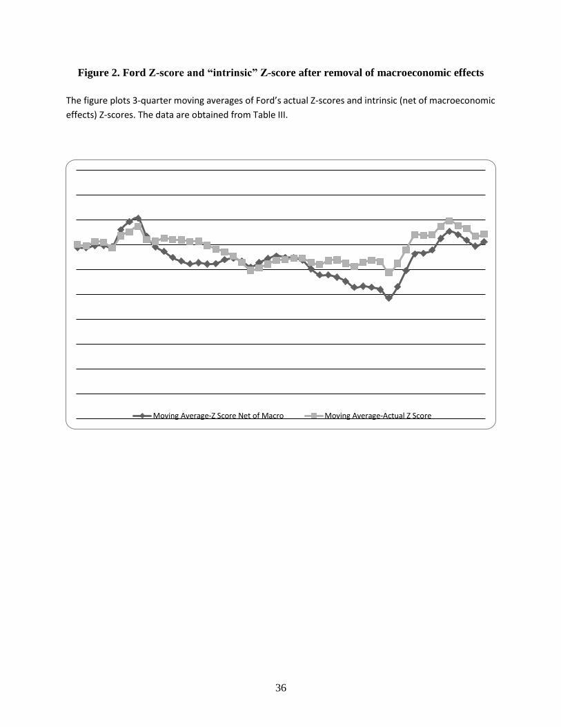
Turning to Ford in Figure 2 it seems that the macro-economy helped Ford “muddle
through” from late 1998 into the year 2000 and, perhaps, even survive the period from the
middle of 2003 until the middle of 2005. During the latter period Ford’s “intrinsic Z-score” fell
to zero before it turned up sharply in the middle of 2005. Thereafter the actual and the intrinsic
Z-score have recovered and followed each other fairly closely up to a level above 1. This level is
still not “safe” but it seems appropriate that Ford’s recent restructuring has been managed
internally by the incumbent management and with less divestment than GM.
The discussion of approaches to restructuring in Section I would lead to the conclusion
that the appropriate action for GM would probably be Chapter 7 bankruptcy in 2008 or earlier.
With the benefit of hindsight we know that a Chapter 11 bankruptcy was engineered by the US
government but it was in many ways similar to a pre-packaged Chapter7 bankruptcy. The old
GM management was replaced, the government took over majority ownership and parts of the
company in “economic distress” were shut down. Thus, the actions taken are very much
consistent with the needs of firms with the intrinsic Z-scores we observe in Figure 1.
One may ask whether the restructuring of Ford initiated by its management in 2005 could
have been initiated already in 2003 if macroeconomic factors had not obscured how close to
bankruptcy Ford was? Similarly, GM’s bankruptcy may have occurred already in 2005 or 2006 if
macroeconomic factors and gasoline price developments, in particular had not contributed to
keeping the bankruptcy indicators from falling until early in 2007.
V. Conclusion
We have here suggested that - in order to improve the reconstruction decision - indicators of the
probability of corporate default, or changes therein, should be decomposed into a
macroeconomic and an intrinsic component with attention paid to the firm-specific character of
the macroeconomic influences. If a declining value of the indicator of default is explained
primarily by macroeconomic factors a reduction in leverage, improved macroeconomic risk
26
management or relatively light assets restructuring may be sufficient to reduce the probability of
default. In case of insolvency, rehabilitation under Chapter 11 with the incumbent management
in place can be an appropriate procedure. If instead the declining value of the indicator is
explained by intrinsic factors, a change of management may be necessary to effectively
implement fundamental asset restructuring. A takeover is one possibility while bankruptcy under
Chapter 7 may be necessary in case of actual insolvency.
The method of decomposition we propose relies on market price variables on the macro-,
industry- and firm levels to obtain coefficients for the sensitivity of the default indicator to
changes in the different price variables. We focus on price variables because they are most
easily, frequently, and quickly observed, and they should be systematically related to the
underlying fundamental factors.
Once the coefficients are estimated, observations of changes in the macro variables can
be used to calculate the total macroeconomic impact on the default indicator for a period. The
remaining change in the indicator during a period is considered caused by intrinsic factors.
Altman’s Z-score was used as the indicator of default probability to illustrate the practical
use of the method. The Z-scores for GM and Ford were calculated and the quarterly changes
from 1996 through the third quarter of 2008 were decomposed into macroeconomic and intrinsic
components. Rising gas prices in 2005 and 2006 seem to have kept GM’s Z-score from falling
even more by increasing its competitiveness relative to Ford and possibly delayed bankruptcy.
Nevertheless, bankruptcy involving management change and substantial divestment of assets
seems to have been an appropriate course of action once it occurred. Ford’s Z-scores seem to
have been kept up by macroeconomic developments that obscured the need for restructuring
during a couple of years before the millennium change and during a period before mid-2005.
Thereafter the actual and intrinsic Z-scores have improved to a level consistent with survival
under the leadership of the incumbent management team. For the two companies in the same
industry and with about the same Z-value in 2005 we end up with different suggested ways of
reconstruction once we take into account the firm-specific macroeconomic influences on the
distress probability.
27
Acknowledgements
We would like to thank Ed Altman for useful comments on this paper. Financial support from
NASDAQ OMX Nordic Foundation (for Lars Oxelheim) is gratefully acknowledged.
References
Allen, L. and A. Saunders, 2004, ”Incorporating Systemic Influences into Risk Measurements: A
Survey of Literature,” Journal of Financial Services Research 26 (No. 2), 161-191.
Altman, E. I.,1968, “Financial Ratios, Discriminant Analysis and the Prediction of Corporate
Bankruptcy,” Journal of Finance 23 (No. 4), 589-609.
Altman, E. I., 2000, Predicting, Financial Distress of Companies: Revisiting the Z-score and
ZETA-models, Personal Homepage, July.
Altman, E. I., 2002, “Corporate Distress Prediction Models in a Turbulent Economy and Basel II
Environment,” Personal homepage, September.
Altman, E. I., 2006, “Are Historically Based Default and Recovery Models in the High-Yield
and Distressed Debt Markets Still Relevant in Today’s Credit Environment?” Special Report,
New York University, Salomon Centre, Stern School of Business, October.
Altman, E. I., B. Brady, A. Resti, and A. Sironi, 2005, “The Link Between Default and
Recovery Rates – Theory, Empirical Evidence and Implications,” Journal of Business 78 (No.
6), 2203-2227.
Altman, E. I. and E. Hotchkiss, 2005, Corporate Financial Distress and Bankruptcy, 3rd
ed.,
New York: Wiley Finance.
Altman, E. I., H. A. Rijken, D. Balan, J. Mina, and M. Watt, 2010, "The Z-Metrics Methodology
for Estimating Company Credit Ratings and Default Risk Probabilities ", MSCI, Inc. Website
and New York University, Salomon Center WP, Stern School of Business, March.
Altman, E. I. and H.A. Rijken, 2011, “Toward a Bottom-Up Approach to Assessing Soveriegn
Default Risk,” Journal of Applied Corporate Finance 23 (No. 1), 20-31.
Black, F. and M. Scholes, 1973, The Pricing of Options and Corporate Liabilities, Journal of
Political Economy 81 (No. 3), 637-654.
28
Carling, K., T. Jacobson, J. Lindé, and K. Roszbach, 2007, Corporate Credit Risk and the Macro
Economy, Journal of Banking and Finance 31 (No. 3), 845-868.
Credit Suisse, 1997, Credit Risk+: A Credit Risk Management Framework. Credit Suisse
Financial Products.
Chava S. and R. Jarrow, 2004, “Bankruptcy Prediction with Industry Effects”, Review of Finance
8 (No. 4), 537-569.
Crouhy, M., D. Galai and R. Mark, 2000, “A comparative analysis of current credit risk models”,
Journal of Banking and Finance 24 (No. 1-2), 59-117.
D’Amato, J. D. and M. Luisi, 2006, “Macro Factors in the Term Structure of Credit Spreads”,
Working Paper, No. 203, Bank for International Settlements, March.
Das, D., P. Homoula, and A. Sarin, 2009, ”Accounting-based versus Market-based Cross-
sectional Models of CDF Spreads”, Journal of Banking and Finance 33 (No. 4), 719-730.
Duffie, D., L. Saita, and K. Wang, 2007, “Multi-period Corporate Default Prediction”, Journal
of Financial Economics 83 (No. 3), 635-665.
Dufresne, C., P. R. Goldstein, and J. S. Martin, 2001, “The Determinants of Credit Spread
Changes”, Journal of Finance 56 (No. 6), 2177-220.
Jacobson, T., R. Kindell, J. Lindé, and K. Roszbach, 2008, “Firm Default and Aggregate
Fluctuations”, Discussion paper 7083, Centre for Economic Policy Research, London.
Jonsson, J. and M. Fridson, 1996, “Forecasting Default Rates on High-yield Bonds”, Journal of
Fixed Income 6 (No. 1), 69-77.
J.P. Morgan, 1997, CreditMetrics: Technical Documentation.
Kealhofer, S., 1995, “Managing Default Risk in Portfolios of Derivatives”, Derivative Credit
Risk, Ch. 4 Risk Publications, 49-66.
Kealhofer, S., 1998, Portfolio Management of Default Risk, Net Exposure 1 (No. 2).
Koopman, S. J., R. Kräussl, A. Lucas, and A. B. Monteiro, 2009, “Credit Cycles and Macro
Fundamentals”, Journal of Empirical Finance 16 (No. 1), 42-54.
Merton, R., 1973, “The Theory of Rational Option Pricing”, Bell Journal of Economics and
Management Science 4 (No. 1), 141-183.
Merton, R., 1974, “On the Pricing of Corporate Debt: The Risk Structure of Interest Rates.”
Journal of Finance 29 (No. 2), 449-470.
29
Oxelheim, L. and C. Wihlborg, 2008, Corporate Decision-Making with Macroeconomic
Uncertainty; Performance and Risk Management, New York: Oxford University Press.
Pesaran, M. H., T. Schuermann, B.-J. Treutler and S. Weiner, 2005,” Global Business Cycles
and Credit Risk” in Carey, M. and R. M. Stultz (eds.) The Risks of Financial Institutions,
Chicago: University of Chicago Press.
Pesaran, M .H., T. Schuermann, B.-J. Treutler and S. Weiner, 2006, “Macroeconomic Dynamics
and Credit Risk,” Journal of Money, Credit and Banking 38 (No. 5), 1211-1261.
Tang, D. Y. and H. Yan, 2010, “Market Conditions, Default Risk and Credit Spreads”, Journal
of Banking and Finance 34 (No. 4), 743-753.
Thorburn, K. S., 2006, “Transparency in Bankruptcy Law: A Perspective on Bankruptcy Costs
across Europe”, in Oxelheim, L. (ed.), Corporate and Institutional Transparency for Economic
Growth in Europe, Oxford, UK: Elsevier, pp. 155-172.
Vasicek, O., 1997, Credit Valuation. Net Exposure 1 (No. 1).
Wihlborg, C., S. Gangopadhyay and Q. Hussain, 2001, “Bankruptcy Infrastructure” in
Brookings-Wharton Papers on Financial Services.
Wilson, T.C., 1997a, Portfolio Credit Risk I, Risk 10 (No. 9), 111-116.
Wilson, T.C., 1997b, Portfolio Credit Risk II, Risk 10 (No. 10), 56-61.
30
Table I Changes in Ford and GM Z-scores, Quarterly, 1996 II – 2008 III
This table shows results of OLS regressions with changes in Z-scores of Ford and GM as dependent
variables. Coefficients with t-values below one were eliminated by stepwise backward elimination of
variables. Figures in parentheses are t-values.
Note: Coefficients in regressions after stepwise backward elimination
Ford GM
Intercept 0.056
(1.04) -0.315
(-1.72) U.S. 3 month Int. Rate,
change - -
Japan 3 month int. Rate,
change - -
Euro 3 month int. Rate,
change - -
U.S. 10 year Int. Rate,
change 0.233
(1.34) 0.225
(1.17) Japanese 10 year Int. Rate,
change -0.290
(-1.11) 10 year Euro Int. Rate,
change -0.293
(-1.31) -
U.S. CPI, % change - 0.847
(2.79)
Japanese CPI, % change -0.156
(-1.68) -0.232
(-2.11) CPI Germany, % change - -
U.S. PPI, % change -0.082
(-1.63) -0.328
(-3.36)
Japanese PPI, % change -0.153
(1.90) -0.296
((2.88)
Euro PPI, % change - -0.300
(-1.83) US gasoline price,
% change - 1.826
(2.52)
Yen/$ % change/100 -1.805
(-2.14) -1.639
(-1.70) Euro/$, % change/100 - -
R square 0.19 0.40
Adjusted R square 0.08 0.26
Observations 50 50
31
Table II. GM Z-score decomposition from 2nd
Quarter 1996-3rd
Quarter 2008.
The table shows how Z-scores and Z-score changes for GM have been decomposed into macroeconomic
and intrinsic components. Column 1 shows the year and quarter for Z-score levels in column 2. Column 3
shows the change of the Z-score from the previous quarter. Column 4 shows the Z-score change caused
by macroeconomic factors. The figures are obtained by multiplication of actual changes in macro-
variables times corresponding coefficients in Table I. Column 5 represents the intrinsic changes in Z-
scores calculated as the difference between columns 3 and 4. Intrinsic changes are accumulated in
column 6 to arrive at Z-score with macroeconomic effects filtered out.
Quarter ending
GM Z-score Level
GM Z-score change
GM Macro change
GM Intrinsic change
GM Z-score net of macro-effect
= Net of accumulated
intrinsic change
1996-2 1.83 0.28 0.49 1.35
1996-3 1.61 -0.22 -0.04 -0.18 1.17
1996-4 1.16 -0.45 0.11 -0.56 0.61
1997-1 1.70 0.54 -0.05 0.58 1.19
1997-2 1.76 0.06 0.17 -0.10 1.09
1997-3 1.55 -0.22 -0.23 0.02 1.10
1997-4 1.03 -0.51 -0.33 -0.18 0.92
1998-1 1.21 0.18 -0.62 0.79 1.72
1998-2 1.18 -0.03 -0.13 0.10 1.81
1998-3 0.96 -0.22 -0.19 -0.03 1.78
1998-4 0.93 -0.03 0.05 -0.08 1.71
1999-1 1.03 0.11 -0.41 0.52 2.22
1999-2 1.09 0.05 0.76 -0.71 1.51
1999-3 0.98 -0.11 0.46 -0.57 0.95
1999-4 0.63 -0.35 0.16 -0.51 0.44
2000-1 0.98 0.35 0.28 0.07 0.51
2000-2 0.98 -0.01 0.32 -0.33 0.18
2000-3 0.84 -0.14 0.02 -0.16 0.03
2000-4 0.93 0.09 -0.15 0.24 0.26
2001-1 0.86 -0.07 -0.13 0.06 0.33
2001-2 0.96 0.11 0.33 -0.23 0.10
2001-3 0.83 -0.13 -0.38 0.25 0.35
2001-4 0.77 -0.06 -0.98 0.92 1.28
2002-1 0.80 0.02 -0.27 0.29 1.57
32
2002-2 0.94 0.15 0.38 -0.24 1.33
2002-3 0.55 -0.39 -0.21 -0.18 1.15
2002-4 0.59 0.04 -0.03 0.06 1.21
2003-1 0.83 0.24 0.44 -0.21 1.01
2003-2 0.92 0.09 -0.22 0.31 1.31
2003-3 0.94 0.02 0.11 -0.09 1.23
2003-4 0.70 -0.23 -0.18 -0.06 1.17
2004-1 0.56 -0.15 0.08 -0.23 0.94
2004-2 0.49 -0.07 0.33 -0.40 0.54
2004-3 0.44 -0.05 -0.11 0.06 0.60
2004-4 0.51 0.07 0.26 -0.19 0.42
2005-1 0.40 -0.11 0.05 -0.16 0.26
2005-2 0.49 0.09 0.24 -0.16 0.10
2005-3 0.55 0.06 0.39 -0.33 -0.23
2005-4 0.17 -0.38 -0.10 -0.29 -0.52
2006-1 1.01 0.84 0.09 0.75 0.23
2006-2 0.72 -0.29 0.61 -0.90 -0.67
2006-3 0.51 -0.21 -0.01 -0.20 -0.87
2006-4 0.64 0.13 -0.63 0.75 -0.12
2007-1 1.05 0.41 -0.01 0.41 0.30
2007-2 1.04 -0.01 0.40 -0.41 -0.11
2007-3 0.57 -0.48 -0.06 -0.42 -0.52
2007-4 0.40 -0.16 0.11 -0.27 -0.79
2008-1 0.53 0.13 0.27 -0.14 -0.93
2008-2 -0.95 -1.48 0.41 -1.88 -2.82
2008-3 0.28 1.22 0.38 0.84 -1.97
Mean 0.829 -0.026 0.045 -0.071 0.528
Std Dev 0.451 0.372 0.335 0.481 0.978
Note: Initial Z-score is assumed to be unaffected by macro-effect. Macro effect includes gasoline price effect.
33
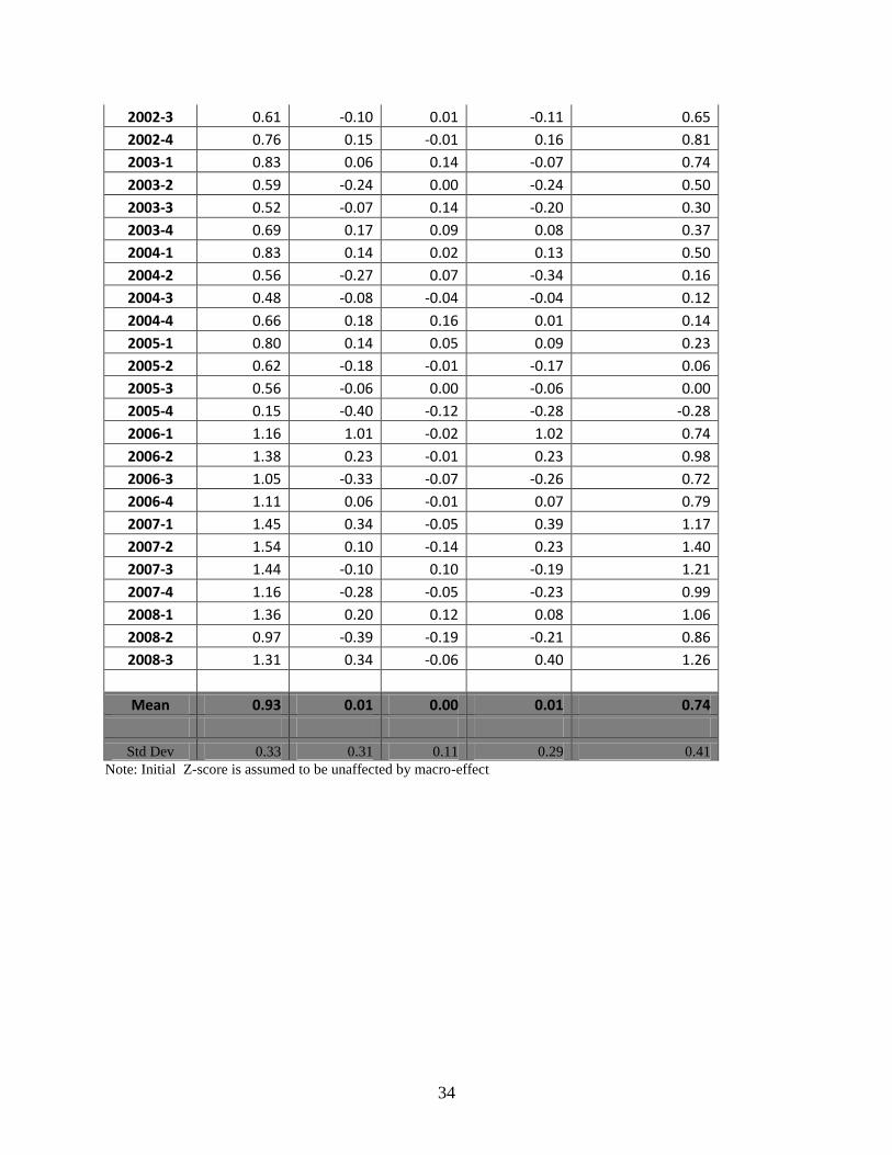
Table III. Ford Z-score decomposition from 2nd
Quarter 1996 - 3rd
Quarter 2008.
The table shows how Z-scores and Z-score changes for Ford have been decomposed into
macroeconomic and intrinsic components. Column 1 shows the year and quarter for Z-score levels in
column 2. Column 3 shows the change of the Z-score from the previous quarter. Column 4 shows the Z-
score change caused by macroeconomic factors. The figures are obtained by multiplication of actual
changes in macro-variables times corresponding coefficients in Table I. Column 5 represents the intrinsic
changes in Z-scores calculated as the difference between columns 3 and 4. Intrinsic changes are
accumulated in column 6 to arrive at Z-score with macroeconomic effects filtered out.
Quarter ending
Ford Z-score Level
Ford Z-score
change
Ford Macro Change
Ford Intrinsic Change
Ford Z-score net of macro-effect = net
of accumulated intrinsic change
1996-2 1.08 0.09 0.07 1.01
1996-3 0.91 -0.17 0.00 -0.16 0.84
1996-4 1.02 0.10 -0.03 0.14 0.98
1997-1 1.01 -0.01 -0.02 0.01 0.99
1997-2 1.15 0.14 0.15 -0.02 0.97
1997-3 0.99 -0.16 -0.18 0.02 0.99
1997-4 0.67 -0.32 -0.23 -0.09 0.91
1998-1 1.87 1.19 0.10 1.09 2.00
1998-2 1.23 -0.64 -0.12 -0.52 1.48
1998-3 0.99 -0.24 0.14 -0.37 1.11
1998-4 1.07 0.08 0.27 -0.19 0.91
1999-1 1.13 0.06 0.13 -0.08 0.84
1999-2 1.18 0.05 0.05 0.00 0.83
1999-3 0.99 -0.19 0.09 -0.28 0.55
1999-4 1.11 0.12 0.05 0.07 0.62
2000-1 1.08 -0.03 -0.08 0.05 0.67
2000-2 1.01 -0.07 -0.02 -0.05 0.62
2000-3 0.85 -0.16 -0.09 -0.07 0.55
2000-4 0.86 0.01 -0.13 0.15 0.69
2001-1 0.85 -0.01 -0.17 0.17 0.86
2001-2 0.58 -0.28 -0.04 -0.23 0.62
2001-3 0.49 -0.09 0.01 -0.11 0.52
2001-4 0.38 -0.11 -0.08 -0.02 0.50
2002-1 0.74 0.36 -0.05 0.40 0.90
2002-2 0.71 -0.03 0.11 -0.13 0.76
34
2002-3 0.61 -0.10 0.01 -0.11 0.65
2002-4 0.76 0.15 -0.01 0.16 0.81
2003-1 0.83 0.06 0.14 -0.07 0.74
2003-2 0.59 -0.24 0.00 -0.24 0.50
2003-3 0.52 -0.07 0.14 -0.20 0.30
2003-4 0.69 0.17 0.09 0.08 0.37
2004-1 0.83 0.14 0.02 0.13 0.50
2004-2 0.56 -0.27 0.07 -0.34 0.16
2004-3 0.48 -0.08 -0.04 -0.04 0.12
2004-4 0.66 0.18 0.16 0.01 0.14
2005-1 0.80 0.14 0.05 0.09 0.23
2005-2 0.62 -0.18 -0.01 -0.17 0.06
2005-3 0.56 -0.06 0.00 -0.06 0.00
2005-4 0.15 -0.40 -0.12 -0.28 -0.28
2006-1 1.16 1.01 -0.02 1.02 0.74
2006-2 1.38 0.23 -0.01 0.23 0.98
2006-3 1.05 -0.33 -0.07 -0.26 0.72
2006-4 1.11 0.06 -0.01 0.07 0.79
2007-1 1.45 0.34 -0.05 0.39 1.17
2007-2 1.54 0.10 -0.14 0.23 1.40
2007-3 1.44 -0.10 0.10 -0.19 1.21
2007-4 1.16 -0.28 -0.05 -0.23 0.99
2008-1 1.36 0.20 0.12 0.08 1.06
2008-2 0.97 -0.39 -0.19 -0.21 0.86
2008-3 1.31 0.34 -0.06 0.40 1.26
Mean 0.93 0.01 0.00 0.01 0.74
Std Dev 0.33 0.31 0.11 0.29 0.41
Note: Initial Z-score is assumed to be unaffected by macro-effect
35
Figure1. GM Z-score and “intrinsic” Z-score after removal of macroeconomic effects
The figure plots 3-quarter moving averages of GM’s actual Z-scores and intrinsic (net of macroeconomic
effects) Z-scores. The data are obtained from Table II.
Moving Average-Z Score Net of Macro Moving Average-Actual Z Score
36
Figure 2. Ford Z-score and “intrinsic” Z-score after removal of macroeconomic effects
The figure plots 3-quarter moving averages of Ford’s actual Z-scores and intrinsic (net of macroeconomic
effects) Z-scores. The data are obtained from Table III.
Moving Average-Z Score Net of Macro Moving Average-Actual Z Score