Core Percolation in Coupled Networks

Jiayu Pan1, Yuhang Yao2, Luoyi Fu2, Xinbing Wang2Department of {Zhiyuan College1, Computer Science2,}, Shanghai Jiao Tong University, China

ABSTRACT

Core percolation, as a fundamental structural transition re-sulted from preserving codes nodes in the network, is crucialin network controllability and robustness. Prior works aremainly based on single, non-interacting network where corenodes are obtained by a classic Greedy Leaf Removal (GLR)procedure that takes off leaf nodes along with their neigh-bors iteratively. Consequently, it remains unknown how suchstructural transition may affect realistic complex systemsthat usually contain multiple interdependent networks.

We take a first look into core percolation in such multi-networks by starting from coupled networks with two fully-interdependent networks. To obtain core nodes in both net-works, we propose a new algorithm, called Alternating GLRprocedure, that recursively switches between networks in car-rying out GLR for node removal. We prove that the pro-posed algorithm can guarantee the uniqueness in the sensethat the final remaining nodes and edges in either of thecoupled networks remain the same, and then present ana-lytical solutions for the fraction of core nodes that will beultimately left when the algorithm terminates. Along withfurther empirical observations, surprisingly, we find that op-posite to the single network that can always guarantee coreemergence after GLR given that the network is sufficientlydense, core can possibly fail to emerge in coupled networksdue to the cascading failure caused by node removal inter-dependence between networks. Also, the presence of coreexhibits a jump at the critical point as a first order tran-sition in coupled networks while it undergoes a continuoussecond order one in a single network.

1 INTRODUCTION

During the past decade, structural transition in complex net-works has received considerable attention, and was manifest-ed its crucial role in many network properties such as robust-ness and resilience to breakdowns [1][2], epidemic and infor-mation spreading on social networks [3][4], social influencepropagation, and the fragility caused by multilayer connec-tions [5]. One type of structural transition belongs to corepercolation. It technically refers to the process of obtainingcore, i.e, a spanned subgraph remained in the network aftera classic greedy leaf removal procedure that removes leaves(nodes of degree one) and its neighbor iteratively, along withthe removal of all their links. As revealed by recent work,the robustness of network controllability relies heavily on thepresence of a core in the network [7]. While core percolationhas been intensively studied in single, non-interacting net-works [6–10], it is still not entirely understood how it mayaffect realistic complex systems, which are usually composedof multiple interdependent networks.

Such network structure is also called network of networks(NoNs) [11][12][13]. Different from a single network, NoNsdescribe the connections and interdependence among multi-ple networks [14]. In other words, the functioning of nodesin one network is dependent upon the functioning of nodesin other networks of the system. Such characteristic, on onehand, can easily lead to the cascading failure where a failureof a very small fraction of nodes in one network may leadto the complete fragmentation of a system of several interde-pendent networks. A typical example belongs the dramaticreal-world cascade of failures, i.e., the electrical blackout thataffected much of Italy on 28 September 2003: the shutdownof power stations directly led to the failure of nodes in the In-ternet communication network, which in turn caused furtherbreakdown of power stations [15]. On the other hand, wheneffectively utilized, multi-interdependence between networkscan also bring about performance gain. Take informationtransmission in conjoined networks [16] for instance. It sug-gests that the fraction of individuals who receive an itemof information is shown to be significantly larger in the con-joint social-physical network case (multiple networks case),as compared to the case where the networks are disjoint (s-ingle network case). The above mentioned phenomenons,leading to either performance degradation or improvemen-t, are closely related to core percolation that characterizeshow local change of the structure may eventually incur aglobal network structural transition. However, existing workregarding NoNs is mainly based on the analysis of giant com-ponent emergence [17][18], whereas core percolation, whichis equally important as noted earlier, has not yet been inves-tigated in NoNs.

We are thus motivated to take a first attempt to study corepercolation in NoNs. Different from a single network, theproblem is made far more complicated in NoNs in the sensethat the existence of intricate multi-interdependence amongnetworks renders it difficult to mathematically characterizethe node removing process. To get a tractable result, we ap-proach the problem by starting from a special case of NoNs,i.e., coupled networks that contain two fully interdependentnetworks, indicating that each node in one network can al-ways find its counterpart in the other network. The resultis extendable to more general forms of NoNs. Recall that acore can be obtained in a single network through convention-al GLR procedure in an iterative fashion, as stated earlier.Here we partially borrow this idea and propose a new noderemoval algorithm that incorporates the mutual influence be-tween networks. Named as Alternating GRL Procedure, themain idea of the algorithm is to firstly choose a network andexecutes in that specific network the GLR procedure, whichcan be reproduced in the following way: A node with degreeone (leaf) is randomly chosen, and removed along with all

its neighbors as well as the links in between. Nodes thatbecomes isolated are also removed. The procedure is repeat-ed until there remain no leaf nodes. The algorithm thenswitches to the other network where it continues the aboveGLR process, from which the removal of nodes will furthercause some nodes to be removed in the first network. Suchprocedure repeats in the prescribed alternating manner tillno nodes can be removed from the whole system. And the fi-nal remaining nodes in coupled networks are thus called corenodes. Additionally, several categories of removable nodes,depending on how they are removed during the algorithm,are also introduced.

While we defer definitions of each node category in Section2.3, we prove that, the proposed algorithm can guarantee theuniqueness in the sense that the final remaining nodes andedges remain the same in terms of node category in bothof the networks, as a fundamental validation of the system.Following that, we proceed to analyze the final fraction ofcore nodes as well as the critical condition under which coreappearance occurs, as a major characteristic of core perco-lation when the number of nodes goes to infinity. This, in-terpreted from a more technical perspective, is to establishiterative equations that captures the dynamic node removalprocess following an alternative fashion in coupled networks.In addition to the fraction of core nodes in each iterative, wealso need to incorporate the node degree distribution changethat affects the calculation at the next iteration. More pre-cisely speaking, at each iteration we need to switch betweennetworks for updating both the fractions of core nodes and n-odal degree distributions. Due to the difficulty in derivationof the exact solution of node degree distribution, we turn toprovide the corresponding approximations.

We disclose from our derivations, along with empirical re-sults of real datasets, that due to the cascading failure, corenodes start to appear at a larger mean degree in coupled net-works than that in a single network. Also, we find that thefraction of final remaining nodes undergoes a jump at thecritical value as a first order phase transition, whereas insingle network it undergoes a continuous second order tran-sition. The reason behind is that in coupled networks, forboth of the networks around a critical state, it seems thatthe nodal degree distribution is close to a power law, thusadding only a few extra nodes with degree one will cause thewhole system to collapse. In addition, we even obtain an in-teresting experimental observation that if the two networksare partially interdependent instead of being fully interde-pendent, there will be equal fractions of remaining nodes inboth networks as long as both of them have the same degreedistributions, regardless of the strength of interdependencebetween two networks.

The algorithm for core nodes acquisition is efficiently im-

plementable, having a complexity of no more than O(N32 ),

with N representing the total number of nodes in each net-work. The complexity stems mainly from the renew of nodaldegree distribution in each iteration, and can be potentiallyreduced through only renewing the node degree distribution

that has higher probabilities. Also, we provide some furtherunderstanding of previously investigated percolation issue incoupled networks.

The rest of the paper is organized as follows. Section 2introduces network model and Section 3 proves the unique-ness of the core percolation in coupled networks. In Section4, we establish iterative equations of the dynamic process ofnode removal and empirically verify our theoretical findingsin Section 6. Section 7 concludes the paper.

2 MODELS AND DEFINITIONS

2.1 Coupled Networks

A general interdependent system consists of multiple net-works, each of which, unlike a traditional single network,establishes connections with some of the other networks inthe system. Each connection is assumed to be in a randommode and each node in a generic network i is supposed tohave equal probability qij to establish connection with somenode in network j. In the present work, we mainly discusscoupled networks that are composed of two interdependen-t networks called networks A and B with equal number ofnodes N . Specifically, we assume that the dependence coef-ficient qAB = qBA = q = 1, meaning that the two networksare fully interdependent. The mutual influence in couplednetworks is revealed in the way that if a node i in networkA depends on a node j in network B, then the removal ofj will also lead to the removal of node i. Although couplednetworks serve as a special case of interdependent networks,the derived results can provide useful guidelines for futureextension to multi-interdependent networks.

This paper mainly discusses the non-feedback condition,whose definition includes three rules: (1) Suppose nodes j,k are both in network B. If node i depends on both j andk, then j = k; (2) Suppose i and l are both in network A. Ifboth i and l depend on j, then i = l. (3) Suppose i dependson k, k depends on l, then i = l.

2.2 A Node Removal Procedure inCoupled Networks

Based on the model stated above, we now introduce the n-ode removal procedure in such networks. Recall that in a sin-gle network, nodes can be removed through the well-knownGreedy Leaf Removal (GLR) algorithm where leaf node, i.e.,node with degree one is randomly chosen and removed a-long with its neighbors, followed by the removal of resultedisolated nodes. The procedure is repeated until no leaf n-odes are left. However, coupled networks differ from a singlenetwork in that the effect of connection between networkscannot be overlooked. Based on that, we introduce belowa new node removal procedure in coupled networks. Specif-ically, we name it Alternating GLR Procedure, whichcontains three major steps:

(1) Node removal in network A: Randomly choose a leafnode in A, and remove this node along with its neighbors.The operation continues until no leaves exist in network A.Isolated nodes in A will then also be removed. This proce-dure resembles the traditional GLR in a single network [10].

1a

3a

3b

2a

2b

1b

A

B

4 5

a ,a removed

by GLR

4 5

b ,b removed

because of A

GLR in B GLR in A 1a

3a

4a

5a

3b

5b

2a

2b

1b

4b

A

B

6 7 8a ,a ,a removed

by GLR

6 7 8b ,b ,b removed

because of A

1a

3a

4a

6a

8a

5a

7a

3b

5b

6b

8b

2a

2b

1b

4b

7b

A

B

Figure 1: Overview of Alternating GLR Procedure in coupled networks. Each node is dependent on a different nodein the other network. Specifically, ∀i ∈ [1 . . . 8], node ai depends on node bi and in return bi depends on ai. Finally nodesa1 − a3 and b1 − b3 become core nodes in networks A and B, respectively. All of the nodes, i.e., removed nodes and core

nodes in A, B are well-defined. Moreover, nodes a7, a8 and b7, b8 are α removable nodes, a4, nodes a6, b4, b6 are β nodesand nodes a5, b5 are γ nodes.

The fraction of remaining nodes in A is denoted as µ1. Thedifference here is that the removed nodes in A will cause theremoval of the corresponding (dependent) nodes in networkB. As illustrated in Fig. 1, we choose network A and operateGLR that causes nodes a6−a8 to be removed. Consequently,nodes b6 − b8 in network B are also removed.

(2) Further node removal in network B: Upon completionof the above GLR in A, the procedure turns to Network Bwhere traditional GLR is further adopted for node removal.Recall that during GLR in A, some nodes in B have alreadybeen removed due to the interdependency between A and B.Similarly, the fraction of remaining nodes in B is denotedas µ2, and the removed nodes in B also cause the furtherremoval of the corresponding nodes in A. Take Fig. 1 as ex-ample. We can see that the removal of nodes b4, b5 furtherleads to the removal of nodes a4, a5.

(3) Alternative Repetition of steps 1 and 2: The above t-wo steps are iteratively repeated in the prescribed alterna-tive manner until no nodes can be removed in both network-s. During the iteration, the fraction of remaining nodes µ3,µ4...can be obtained. Specifically, till the n + 1th iteration,in network A, we have obtained µ1, µ3, µ5,. . .,µ2n+1 withodd subscripts while for network B, we have obtained µ2,µ4, µ6,. . .,µ2n+2 with even subscripts. We denote by µ∞,1

and µ∞,2 respectively the fraction of final remaining nodes innetworks A and B. Since the system is fully interdependent,it is apparent that µ∞,1 = µ∞,2 = µ∞.

The overview of the whole Alternating GLR Procedure isalso illustrated in Fig. 1. In consistency with previous works,here we also introduce the conception of core percolation,defined as the phenomenon of structural transition resultedfrom the algorithm when the number of nodes goes to infinity,which is our major concern of this work.

2.3 Categorization of Node Types

To systematically study core percolation on coupled network-s, we classify the nodes into two major categories accordingto how they can be removed during the above AlternatingGLR procedure:

1. Core nodes: Analogous to a single network wherethe remaining nodes are called core nodes [10], in couplednetworks, the remaining nodes after Alternating GLR arealso called core nodes. In Fig. 1, nodes a1 − a3 and b1 − b3are core nodes in networks A and B, respectively.

2. Removable nodes: similar to a single network [10],the removable nodes can be further classified into three types:α removable nodes which can be isolated without directlyremoving themselves, β removable nodes which can be theneighbor of a leaf node and γ nodes which are removable butmeanwhile neither α nor β removable.

Furthermore, as we will also demonstrate in Section 3, aslong as the node removal follows the proposed algorithm,both the remaining nodes and edges, belonging to eithercore nodes or three types of removable nodes in networks Aand B, are well-defined, a phenomenon that is alternativelycalled uniqueness indicating that the remaining nodes andedges remain the same in terms of node type under differentremoving sequences which all follow the common frameworkof the proposed algorithm.

The interplay among nodes of different types can be inter-preted in a more detailed way. According to the behaviorsof Alternating GLR algorithm, when it is executed in net-work A, the node removal process resembles the traditionalGLR in a single network. According to the algorithm, re-moved nodes will cause corresponding nodes in network Bto be removed. To remain the aforementioned uniqueness,the corresponding removed nodes in network B are classifiedas the same with the dependent nodes in network A. As ex-emplified in Fig. 1, the definitions of nodes b6 − b8 are thesame with their dependent nodes. As a result, nodes b7, b8are α nodes and node b6 is β node, regardless of their roles innetwork B. Similarly, when GLR is operated in network B,the corresponding nodes in network A are classified as thesame with dependent nodes in B. For instance, if node a1 inA is removed and classified as α removable, and node b2 innetwork B depends on node a1, then b2 is also α removable.

Table 1 lists the main notations that will be used through-put the paper.

Notation DefinitionG an undirected graphP (k) probability of a node with degree kG(z) generating function of a graphµ fraction of core nodes in one iterationqij the number of nodes in network j that depend on

network i divided by total number of nodes in network jc mean degree of nodesg(G(z)) fraction of core nodes of a graph with G(z)f(G(z)) the generating function after operating GLR

in a graph with G(z)

Table 1: Notions and Definitions

3 UNIQUENESS OF COREPERCOLATION

In this section, we prove that when the algorithm terminates,each type of nodes (See Section 2.3) are well-defined in cou-pled networks.

3.1 Reasonability of the Algorithm

A major characteristic of our algorithm is that before itswitches to the other network (without loss of generality,here we can say network B), it will continue the executionof GLR in the original network (say network A) until thereare no more nodes that can be removed from that network.As a seemingly feasible alternative, this constraint can beloosened by letting the algorithm switch to network B for anew GLR execution before it finishes the original GLR pro-cedure in network A. However, as we will illustrate in theexample below, such change will not guarantee the unique-ness.

1a

3a

4a

7a

3b

2a

2b

1b

4b

7b

A

B

1a

3a

3b

2a

2b

1b

A

B

5 6

:

,

GLR at half

only remove a a GLR in our model

1a

3a

4a

6a

5a

7a

3b

5b

6b

2a

2b

1b

4b

7b

A

B

Figure 2: Difference between using GLR process to theend and using GLR process at half before applying it to

another network. According to Alternating GLR proce-dure, the core nodes are shown on the right lower side ofthe figure. If we loosen our restriction, the condition will

be different, and the uniqueness will not be guaranteed.

We take Fig. 2 for example to explain why the unique-ness cannot be guaranteed in such case. In the figure, ∀i ∈[1 . . . 7], node ai depends on node bi and in return bi dependson ai. The nodes on the right lower figure are remaining n-odes according to our algorithm. However, if we remove onlya part of the removable nodes in network A and then switchto network B for the new GLR, the final remaining nodesin the two networks will be different from those obtainedpreviously. The left lower part of the figure exemplifies suchpossibility. Here the algorithm only removes nodes a5, a6from network A, and then turns to network B to start a newGLR procedure. As a result, node b3 is removed since it is aneighbor of the leaf node b4. In the end, all of the nodes inthe system will be removed, leading to a total cascade failure.This outcome is quite different from the former one wherethere are same remaining nodes and edges left in couplednetwork. This implies that it is reasonable to stick to onenetwork to finish the whole GLR process before it switchesto the other one for a new GLR. In addition, it is worthwhile

noting that the choice of A or B for GLR operation at firstwill lead to different remaining nodes in two networks, evenif µ∞ for the two networks will be the same.

3.2 Uniqueness of Core Percolation

With the clarification of the reasonability of the algorithm,we are now ready to prove the uniqueness property. Since weare considering core percolation in coupled networks, provingthe uniqueness in coupled networks is equivalent to provingthat it is unique in either of the networks. Here the proofin either network of the coupled networks also includes twoparts, i.e., to prove that both the core nodes and removablenodes obtained under our algorithm are unique. The follow-ing theorem states a uniqueness guarantee in either of thenetwork in the coupled ones.

Theorem 3.1. Regardless of the different sequences ofGLR node removal procedures, the remaining nodes and edgesremain the same.

Proof. Without loss of generality, we focus on networkA in coupled networks. The proof is divided into two steps:(1) proving the uniqueness of the core nodes, and (2) provingthe uniqueness of removable nodes, as stated above. Now wefocus on the first step as follows:

1. The uniqueness of core nodes: According tothe behavior of Alternating GLR procedure, it adopts tra-ditional GLR when it is in the progress of node removal inone specific network. Now suppose in network A, there existtwo different GLR sequences called GLR1 and GLR2, wherea node v becomes a core node after the execution of GLR1,but meanwhile not a core node resulted from GLR2. Then,proving Theorem 1 is equivalent to proving that such kindof node v does not exist.

First, we take a look at GLR2, where we know that node vis removed after some steps due to one of the three followingconditions:

(i) v is a leaf, thus it will be removed at the next step;(ii) v is a neighbor of a leaf;(iii) v becomes isolated.

Now we prove that v cannot be a core node in GLR1 in anyof the three conditions.

(i) If v is a leaf, the neighbor nodes of v must be removedsince they are also the neighbors of other leaves. We denoteone of v’s neighbors as n1, and one of n1’s another neighborsas v1, which is also a leaf that can link to other nodes similarto itself. Following the same manner, we can find a seriesof nodes denoted as n2, v2, ... located on a path. Noticethat v and n are staggered. If the path, after some steps,finds that its point belongs to this path, then this path willstep back one point and find another link to go along. Inthis way, every bifurcation can stretch and end up to a leafwithout incurring a cycle. If one of v’s links cannot find anon-cycled path, then this cycled path will not be removedunder any circumstances. Hence we can find such kind ofnon-cycled path, the end of which is a leaf.

Now we take a look back into GLR1, where v is a corenode and may undergo many bifurcations before. Since v

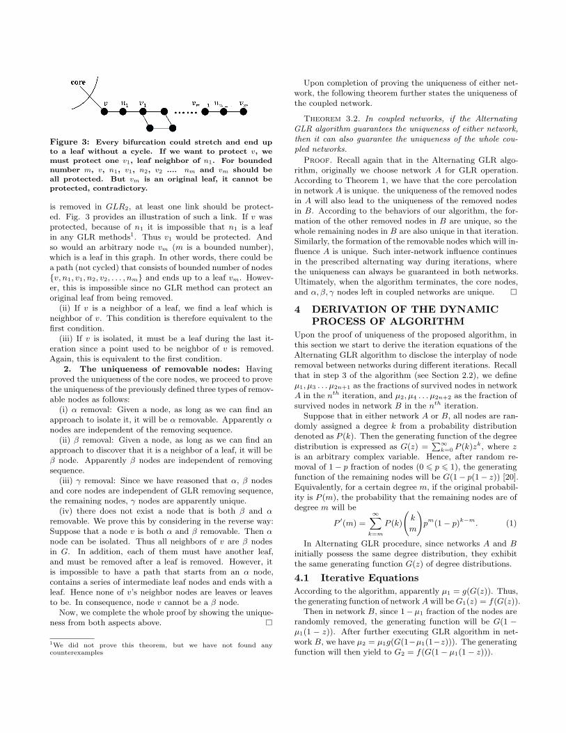
Figure 3: Every bifurcation could stretch and end upto a leaf without a cycle. If we want to protect v, we

must protect one v1, leaf neighbor of n1. For boundednumber m, v, n1, v1, n2, v2 .... nm and vm should beall protected. But vm is an original leaf, it cannot beprotected, contradictory.

is removed in GLR2, at least one link should be protect-ed. Fig. 3 provides an illustration of such a link. If v wasprotected, because of n1 it is impossible that n1 is a leafin any GLR methods1. Thus v1 would be protected. Andso would an arbitrary node vm (m is a bounded number),which is a leaf in this graph. In other words, there could bea path (not cycled) that consists of bounded number of nodes{v, n1, v1, n2, v2, . . . , nm} and ends up to a leaf vm. Howev-er, this is impossible since no GLR method can protect anoriginal leaf from being removed.

(ii) If v is a neighbor of a leaf, we find a leaf which isneighbor of v. This condition is therefore equivalent to thefirst condition.

(iii) If v is isolated, it must be a leaf during the last it-eration since a point used to be neighbor of v is removed.Again, this is equivalent to the first condition.

2. The uniqueness of removable nodes: Havingproved the uniqueness of the core nodes, we proceed to provethe uniqueness of the previously defined three types of remov-able nodes as follows:

(i) α removal: Given a node, as long as we can find anapproach to isolate it, it will be α removable. Apparently αnodes are independent of the removing sequence.

(ii) β removal: Given a node, as long as we can find anapproach to discover that it is a neighbor of a leaf, it will beβ node. Apparently β nodes are independent of removingsequence.

(iii) γ removal: Since we have reasoned that α, β nodesand core nodes are independent of GLR removing sequence,the remaining nodes, γ nodes are apparently unique.

(iv) there does not exist a node that is both β and αremovable. We prove this by considering in the reverse way:Suppose that a node v is both α and β removable. Then αnode can be isolated. Thus all neighbors of v are β nodesin G. In addition, each of them must have another leaf,and must be removed after a leaf is removed. However, itis impossible to have a path that starts from an α node,contains a series of intermediate leaf nodes and ends with aleaf. Hence none of v’s neighbor nodes are leaves or leavesto be. In consequence, node v cannot be a β node.

Now, we complete the whole proof by showing the unique-ness from both aspects above. �

1We did not prove this theorem, but we have not found anycounterexamples

Upon completion of proving the uniqueness of either net-work, the following theorem further states the uniqueness ofthe coupled network.

Theorem 3.2. In coupled networks, if the AlternatingGLR algorithm guarantees the uniqueness of either network,then it can also guarantee the uniqueness of the whole cou-pled networks.

Proof. Recall again that in the Alternating GLR algo-rithm, originally we choose network A for GLR operation.According to Theorem 1, we have that the core percolationin network A is unique. the uniqueness of the removed nodesin A will also lead to the uniqueness of the removed nodesin B. According to the behaviors of our algorithm, the for-mation of the other removed nodes in B are unique, so thewhole remaining nodes in B are also unique in that iteration.Similarly, the formation of the removable nodes which will in-fluence A is unique. Such inter-network influence continuesin the prescribed alternating way during iterations, wherethe uniqueness can always be guaranteed in both networks.Ultimately, when the algorithm terminates, the core nodes,and α, β, γ nodes left in coupled networks are unique. �

4 DERIVATION OF THE DYNAMICPROCESS OF ALGORITHM

Upon the proof of uniqueness of the proposed algorithm, inthis section we start to derive the iteration equations of theAlternating GLR algorithm to disclose the interplay of noderemoval between networks during different iterations. Recallthat in step 3 of the algorithm (see Section 2.2), we defineµ1, µ3 . . . µ2n+1 as the fractions of survived nodes in networkA in the nth iteration, and µ2, µ4 . . . µ2n+2 as the fraction ofsurvived nodes in network B in the nth iteration.

Suppose that in either network A or B, all nodes are ran-domly assigned a degree k from a probability distributiondenoted as P (k). Then the generating function of the degreedistribution is expressed as G(z) =

∑∞k=0 P (k)zk, where z

is an arbitrary complex variable. Hence, after random re-moval of 1− p fraction of nodes (0 6 p 6 1), the generatingfunction of the remaining nodes will be G(1− p(1− z)) [20].Equivalently, for a certain degree m, if the original probabil-ity is P (m), the probability that the remaining nodes are ofdegree m will be

P ′(m) =

∞∑k=m

P (k)

(k

m

)pm(1− p)k−m. (1)

In Alternating GLR procedure, since networks A and Binitially possess the same degree distribution, they exhibitthe same generating function G(z) of degree distributions.

4.1 Iterative Equations

According to the algorithm, apparently µ1 = g(G(z)). Thus,the generating function of networkA will beG1(z) = f(G(z)).

Then in network B, since 1− µ1 fraction of the nodes arerandomly removed, the generating function will be G(1 −µ1(1 − z)). After further executing GLR algorithm in net-work B, we have µ2 = µ1g(G(1−µ1(1−z))). The generatingfunction will then yield to G2 = f(G(1− µ1(1− z))).

With such iterations repeating in the above prescribedway, up to the (n−1)th iterations we have obtained µ2n−1, µ2n

as well as the generating functions of both networks A andB, i.e., G2n−1 and G2n. In the nth iterations, for network A,it should firstly randomly remove a (µ2n−1−µ2n) fraction ofnodes. Then the relative remaining fraction becomes µ2n

µ2n−1,

and the generating function thus becomesG2n−1

(1− µ2n

µ2n−1(1− z)

).

After the GLR process, the equation can be expressed as

µ2n+1 = µ2ng

[G2n−1

(1− µ2n

µ2n−1(1− z)

)]. (2)

Similarly, in the iteration, a fraction (1− µ2n+1/µ2n) of theremaining nodes in network B should be removed. The gen-

erating function will be G2n

(1− µ2n+1

µ2n(1− z)

). After the

execution of GLR in network B, we have

µ2n+2 = µ2n+1g

[G2n

(1− µ2n+1

µ2n(1− z)

)]. (3)

In order to maintain the iteration, the generating functionsshould be updated from G2n−1, G2n to G2n+1, G2n+2, respec-tively.

In each iteration, both the generating functions in net-works A and B will undergo two changes. The first changeresults from random node removal while the second one isincurred by GLR process. Based on the definition, the newiteration equations are

G2n+1(z) = f

[G2n−1

(1− µ2n

µ2n−1(1− z)

)](4)

and

G2n+2(z) = f

[G2n

(1− µ2n+1

µ2n(1− z)

)]. (5)

Here the four parameters µ2n+1, µ2n+2, G2n+1, G2n+2 willkeep being updated until the algorithm converges. And whenn is sufficiently large, we have that µ2n+1 = µ2n+2 = µ∞.Since a monotonous and bounded sequence must convergeto a unique number, there exists only one µ∞. Therefore,obviously we have

limn→∞

G2n−1

(1− µ2n

µ2n−1(1− z)

)= lim

n→∞G2n−1(z), (6)

and

limn→∞

G2n

(1− µ2n+1

µ2n(1− z)

)= lim

n→∞G2n(z). (7)

For the ease of understanding, Fig. 4 shows the overall dia-gram of our derivation. Initially, both networks have µ0 = 1fraction of nodes and µ0 becomes µ1 due to GLR. Next, re-moving a fraction µ0 − µ1 of nodes in network A will causesome nodes in network B to be removed. This, interpret-ed technically, is that the generating function (probabilitydistribution) G1 influences G0 in network B and changes itinto G′

0. After GLR operation in network B, G′0 further be-

comes G2 and fraction of core nodes yields to µ2. Then, G2

changes G1 to G′1 which further becomes G3 after GLR. Fol-

lowing this route, in the nth iteration, G2n−1 is influencedby G2n to G′

2n−1, after GLR, it becomes G2n+1, based onwhich µ2n+1 can be calculated. In analogy, in network B,

Figure 4: Diagram of the derivation of our model.

G2n becomes G2n+2 and µ2n+2 can also be calculated. Insummary, in each iteration, we should update µ2n+1, µ2n+2

as well as the degree distributions of networks A and B.

Remark 1. The proof in previous section indicates thatboth networks A and B possess the same remaining core n-odes. Actually, it is worthwhile noting that in non-feedbackcondition considered in the present work, even if we relaxthe assumption of full interdependence between networks (re-move the constraint of q = 1), the number of core nodes forboth networks will always remain the same as long as theinitial degree distributions are the same in networks A andB. This conclusion, on the first sight, does not appear to beapparent since it is supposed in the algorithm that networkA is chosen first for GLR operation, and either choice of Aor B will destroy the symmetry of the system, possibly forthe non-connecting part, i.e., 1− q of both networks, leadingto the different remaining core nodes. Notice that if q = 1,which is exactly the case we analyze in the paper, the resultis demonstrated to be true; if q = 0, the network is reduced tothe traditional single network, where the result is obviouslytrue again; For other cases in between, suppose we introducea slight increase of q. Then it seems that whether networkA or B loses more nodes is irrelevant to q. Therefore, thedifference of the number of core nodes will increase with asq decreases. However, the difference is still zero when q = 0,verifying the conclusion that the core nodes always remainthe same in networks A and B.

4.2 Solutions of Iterative Equations

After establishing the iterative equations, now we need toseek for the solutions of the two functions, i.e., g(G(z)) andf(G(z)) in the equations.

4.2.1 Solution of Fraction of Core Nodes g(G(z)). As de-fined earlier, g(G(z)) represents the faction of remaining corenodes in each of the coupled networks when the algorithmterminates. Inspired from prior work of traditional singlenetwork [21], we obtain the solution of g(G(z)) with themain idea presented below:

Let α′ (or β′) denote the probability that a random neigh-bor of a random node i in network G is α removable (or β

removable) in network G/i where node i and all of its linksare removed. In particular, node i is α removable in G if allits neighbor nodes are β removable in G/i and β removablein G if at least one neighbor is α removable in G/i. Basedon that, we have

α′ = H(1− β′), 1− β′ = H(α′), (8)

where H(x) = 1c

∑∞k=0(k + 1)P (k + 1)(1 − x)k. Defining

f(x) = H(H(x))− x, we have that α′ is the root of f(x) =0. In the iterative mode, the initial point is x = 0, andaccording to the shape of f(x), the iteration will convergeto its smallest fixed point. We want the smallest root off(x) = 0. After solving α′, β′ = 1 − A(α′), the solutionof the fraction of core nodes ncore in each of the couplednetwork is

ncore =

∞∑k=0

P (k)

k∑s=2

(k

s

)(β′)k−s(α′)s. (9)

According to binomial theorem,

ncore = G(1− α′)−G(β′)− c(1− α′ − β′)α′. (10)

We need to be aware that here α′, β′ are not the same asthe fractions of α, β removable nodes in a traditional singlenetwork. The purpose of introducing α′, β′ is to solve ncore

conveniently. And the the number of α and β nodes, i.e., nα

and nβ , can also be solved by α′ and β′.

4.2.2 Solution of Updated Generating Function f(G(z)).With the solution of G(g(z)), we turn to seek for the solu-tion of updated generating function f(G(z)) of the numberof core nodes. A typical previous methodology to get thesolution [22] is using iteration function, where, however, it-erations are required for every step of leaf node removal,and consequently makes it far more complicated to establishthe equations for every step and relatively difficult to com-pute the process. In addition, since it is impossible to getderivations for many different kinds of graphs, we get aroundthe difficulty by approximating a generating function ratherthan solving it exactly. In other words, we aim to find anapproximate degree distribution of f(G(z)).

According to the algorithm, after GLR operation, nodeswith degrees 1 and 0 are removed, leading to the removalof those with higher degrees in the next iteration. Obvious-ly, the number of nodes with degree 2 will incur the mostchanges. Therefore, our approximation method is to deleteP (0), P (1) and add some part of P (2). Moreover, we knowthat if P (1) is very small, meaning that very few number ofnodes are removed, then it will not incur too much changeto the degree distribution. Under such circumstance, it canbe seen that the change of degree distribution relies heavilyon P (2). Taking into consideration of those conditions, nowwe introduce an index qq satisfying qq > 1. And for a net-work with generating function G(z), after GLR, the updateddegree distribution, denoted as G′(z), should be

G′(z) =1

a

(∞∑

k=3

P (k)zk + P (2)(1 + qq × P (1))z2), (11)

where the normalization number a satisfies

a =

∞∑k=3

P (k) + P (2)(1 + qq × P (1)). (12)

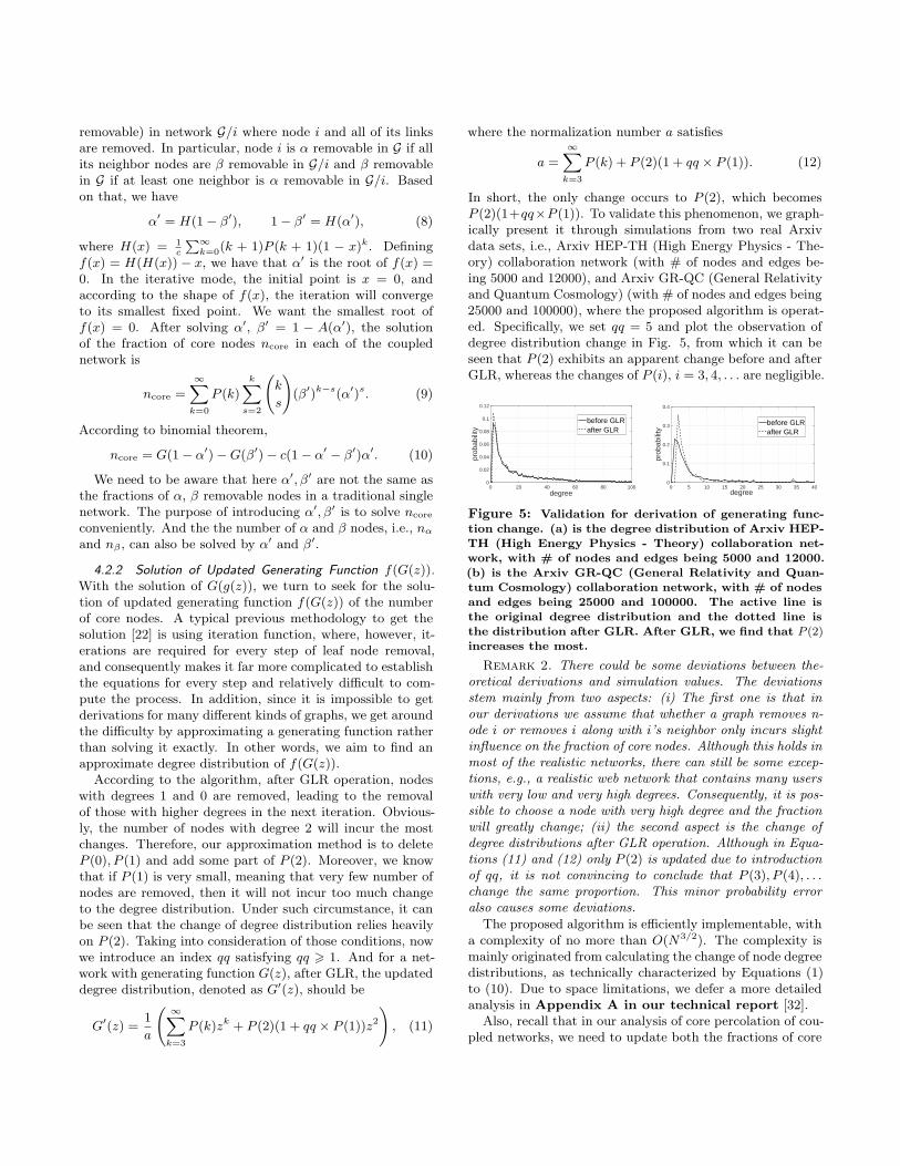
In short, the only change occurs to P (2), which becomesP (2)(1+qq×P (1)). To validate this phenomenon, we graph-ically present it through simulations from two real Arxivdata sets, i.e., Arxiv HEP-TH (High Energy Physics - The-ory) collaboration network (with # of nodes and edges be-ing 5000 and 12000), and Arxiv GR-QC (General Relativityand Quantum Cosmology) (with # of nodes and edges being25000 and 100000), where the proposed algorithm is operat-ed. Specifically, we set qq = 5 and plot the observation ofdegree distribution change in Fig. 5, from which it can beseen that P (2) exhibits an apparent change before and afterGLR, whereas the changes of P (i), i = 3, 4, . . . are negligible.

degree0 20 40 60 80 100

prob

abili

ty0

0.02

0.04

0.06

0.08

0.1

0.12

before GLRafter GLR

degree0 5 10 15 20 25 30 35 40

prob

abili

ty

0

0.1

0.2

0.3

0.4

before GLRafter GLR

Figure 5: Validation for derivation of generating func-tion change. (a) is the degree distribution of Arxiv HEP-

TH (High Energy Physics - Theory) collaboration net-work, with # of nodes and edges being 5000 and 12000.(b) is the Arxiv GR-QC (General Relativity and Quan-tum Cosmology) collaboration network, with # of nodes

and edges being 25000 and 100000. The active line isthe original degree distribution and the dotted line isthe distribution after GLR. After GLR, we find that P (2)increases the most.

Remark 2. There could be some deviations between the-oretical derivations and simulation values. The deviationsstem mainly from two aspects: (i) The first one is that inour derivations we assume that whether a graph removes n-ode i or removes i along with i’s neighbor only incurs slightinfluence on the fraction of core nodes. Although this holds inmost of the realistic networks, there can still be some excep-tions, e.g., a realistic web network that contains many userswith very low and very high degrees. Consequently, it is pos-sible to choose a node with very high degree and the fractionwill greatly change; (ii) the second aspect is the change ofdegree distributions after GLR operation. Although in Equa-tions (11) and (12) only P (2) is updated due to introductionof qq, it is not convincing to conclude that P (3), P (4), . . .change the same proportion. This minor probability erroralso causes some deviations.

The proposed algorithm is efficiently implementable, witha complexity of no more than O(N3/2). The complexity ismainly originated from calculating the change of node degreedistributions, as technically characterized by Equations (1)to (10). Due to space limitations, we defer a more detailedanalysis in Appendix A in our technical report [32].

Also, recall that in our analysis of core percolation of cou-pled networks, we need to update both the fractions of core

nodes and nodal degree distributions. As a counterpart ofcore percolation, percolation theory has also been adoptedto study the vulnerability of coupled networks in previousliterature [11], where, however, only the fraction of nodes ingiant component are updated at each iteration. As a result,it is interesting to have an extra exploration of why the de-gree distribution does not need to be renewed in that case.We defer the details to Appendix B in our technicalreport [32] again due to space limitations.

5 EXPERIMENTS

In this section, we verify our theoretical findings throughexperiments on different real data sets. Specifically, our ex-periments include two parts: (i) observing ncore in both s-ingle network and coupled networks, and (ii) observing thefractions of remaining nodes µ∞ in coupled networks.

5.1 Observation of Core Percolation

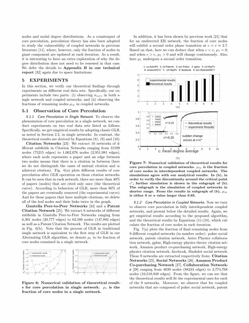
5.1.1 Core Percolation in Single Network. To observe thephenomenon of core percolation in a single network, we con-duct experiments on two real data sets listed as follows.Specifically, we get empirical results by adopting classic GLR,as noted in Section 2.2, in single networks. In contrast, thetheoretical results are derived by Equations (8), (9) and (10).

Citation Networks [23]: We extract 10 networks of d-ifferent subfields in Citation Networks ranging from 31599nodes (75215 edges) to 1,062,076 nodes (2,951,981 edges),where each node represents a paper and an edge betweentwo nodes means that there is a citation in between (herewe do not distinguish the cases of mutual citation and u-nilateral citation). Fig. 6(a) plots different results of corepercolation after GLR operation on those citation networks.It can be seen that in each network, there are more than 40%of papers (nodes) that are cited only once (the theoreticalcurve). According to behaviors of GLR, more than 80% ofthe papers are eventually removed (the experimental curve).And for those papers that have multiple citations, we deleteall of the leaf nodes and their links twice in the graph.

Gnutella Peer-to-Peer Networks [24] and a PatentCitation Network [25]: We extract 6 networks of differentsubfields in Gnutella Peer-to-Peer Networks ranging from6,301 nodes (20,777 edges) to 62,586 nodes (147,892 edges)as well as a Patent Citation Network. The results are plottedin Fig. 6(b). Note that the process of GLR in traditionalsingle network is equivalent to the first step of GLR in ourAlternating GLR algorithm, we denote µ1 to be fraction ofcore nodes remained in a single network.

0 2 4 6 8 10

1: fra

ctio

n of

cor

e no

des

0.3

0.4

0.5

0.6

0.7

0.8

0.9

experimental results

theoretical results

1 2 3 4 5 6 7

1: fra

ctio

n of

cor

e no

des

10-4

10-3

10-2

10-1

100

experimental resultstheoretical results

Figure 6: Numerical validation of theoretical result-s for core percolation in single network. µ1 is thefraction of core nodes in a single network.

In addition, it has been shown by previous work [21] thatfor an undirected ER network, the fraction of core nodeswill exhibit a second order phase transition at c = e ≈ 2.7.Based on that, here we can deduce that when c < e, µ1 = 0;and when c > e, µ1 > 0 and will change continuously. Also,here µ1 undergoes a second order transition.

1 2 3 4 5 6 7 8 90

0.2

0.4

0.6

0.8

1

experimental resultstheoretical results

1: ca-AstroPh 2: cit-Patents 3: soc-Pokec 4: gplus 5: cit-HepTh

(a)

c: mean degree average0 1 2 3 4 5 6 7 8 9 10

0

0.2

0.4

0.6

0.8

1

theoretical resultsexperiment Results

5 5.1 5.2 5.3 5.4 5.50

0.2

0.4

0.6

0.8

1

10000200004000080000

c*=5.25

c*=5.25 sudden changeoccurs at c=c*

(b)

Figure 7: Numerical validation of theoretical results forcore percolation in coupled networks. µ∞ is the fractionof core nodes in interdependent coupled networks. The

simulations agree with our analytical results. In (b), inorder to verify the discontinuity around the critical pointc∗, further simulation is shown in the subgraph of (b).The subgraph is the simulation of coupled networks in

shorter range. From the results in subgraph of (b), µ∞is either 0 or a value larger than 0.65.

5.1.2 Core Percolation in Coupled Networks. Now we turnto observe core percolation in fully interdependent couplednetworks, and present below the detailed results. Again, weget empirical results according to the proposed algorithm,and the theoretical results by Equations (1)-(10), which cal-culate the fraction of core nodes in each iteration.

Fig. 7(a) plots the fraction of final remaining nodes from9 different coupled networks (in number order): pokec socialnetwork, patent citation network, Astro Physics collabora-tion network, gplus, High-energy physics theory citation net-work, Amazon product co-purchasing network, High-energyphysics citation network, facebook, Slashdot social network.These 9 networks are extracted respectively from: CitationNetworks [25], Social Networks [26], Amazon ProductCo-purchasing Network [27], Collaboration Network-s [28] ranging from 4039 nodes (88234 edges) to 3,774,768nodes (16,518,948 edges). From the figure, we can see thatthe theoretical results well fit the experimental ones for eachof the 9 networks. Moreover, we observe that for couplednetworks that are composed of pokec social network, patent

citation network and Astro Physics collaboration network,respectively, there is zero fraction of remaining core nodeswhen the algorithm terminates.

To gain a more clear understanding of phase transition,we also plot in Fig. 7(b) the fraction of core nodes obtainedunder an ER network versus different values of mean degree c.Surprisingly, here µ∞ can remain to be zero even if c > e =2.7. Such occurrence is attributed to the property of cascadefailure in coupled networks. That is to say, if there are noconnections between two networks, it will be reduced to thesingle network and core nodes will appear at the criticalpoint e = 2.7. However, in interdependent networks, a lot ofcore nodes in one of the networks will be removed because ofthe influence from the other one. Under such circumstance,even if c > e, the whole coupled networks can still possiblyundergo a total cascade failure, meaning that the failure of afew nodes in a network will lead to the collapse of the wholesystem. Particularly, in our simulation, we observe that atthe point c = 5, µ1 is about 0.9, a value close to 1. However,ultimately, µ∞ is still 0.

In the figure, there is a clear phase transition at the pointc∗ = 5.25, where the fraction of core nodes undergoes anabrupt change from 0 to around 0.7. At this point, as the to-tal number of nodes N increases, µ∞ also exhibits a gradualincrease following the form of a ladder function. Therefore,it is persuasive to say that when N goes to infinity, µ∞ willexhibit a sudden change. This condition concludes that atthe critical point c∗, µ∞ is discontinuous, meaning that µ∞undergoes a first order phase transition.

Comparison between single and coupled networks:Prior work has demonstrated that in a single network, forsimilar kinds of networks, the number of core nodes ncore

will be zero if c is small but be larger than zero when c be-comes large. In that case, the ncore will change continuouslyat the critical point, which is a second order phase transition.However, when it comes to coupled networks, at a criticalpoint which is larger than that in a single network, the frac-tion of core nodes µ∞ will change discontinuously, which isa first order transition. Furthermore, in interdependent net-works, even if c is very large, the networks will still have alarge chance of collapse. Another example is the generatingnetwork, where an initial removal of a few nodes will causethe coupled system to break down ultimately.

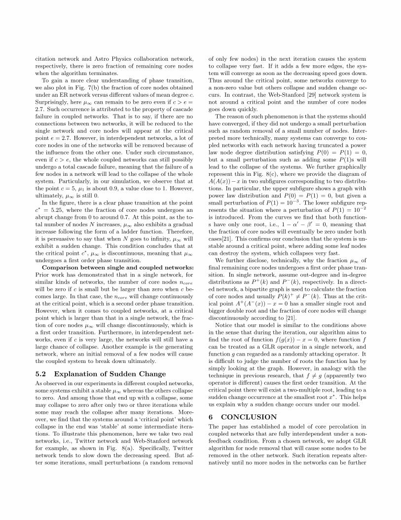
5.2 Explanation of Sudden Change

As observed in our experiments in different coupled networks,some systems exhibit a stable µ∞ whereas the others collapseto zero. And among those that end up with a collapse, somemay collapse to zero after only two or three iterations whilesome may reach the collapse after many iterations. More-over, we find that the systems around a ‘critical point’ whichcollapse in the end was ‘stable’ at some intermediate itera-tions. To illustrate this phenomenon, here we take two realnetworks, i.e., Twitter network and Web-Stanford networkfor example, as shown in Fig. 8(a). Specifically, Twitternetwork tends to slow down the decreasing speed. But af-ter some iterations, small perturbations (a random removal

of only few nodes) in the next iteration causes the systemto collapse very fast. If it adds a few more edges, the sys-tem will converge as soon as the decreasing speed goes down.Thus around the critical point, some networks converge toa non-zero value but others collapse and sudden change oc-curs. In contrast, the Web-Stanford [29] network system isnot around a critical point and the number of core nodesgoes down quickly.

The reason of such phenomenon is that the systems shouldhave converged, if they did not undergo a small perturbationsuch as random removal of a small number of nodes. Inter-preted more technically, many systems can converge to cou-pled networks with each network having truncated a powerlaw node degree distribution satisfying P (0) = P (1) = 0,but a small perturbation such as adding some P (1)s willlead to the collapse of the systems. We further graphicallyrepresent this in Fig. 8(c), where we provide the diagram ofA(A(x))−x in two subfigures corresponding to two distribu-tions. In particular, the upper subfigure shows a graph withpower law distribution and P (0) = P (1) = 0, but given asmall perturbation of P (1) = 10−3. The lower subfigure rep-resents the situation where a perturbation of P (1) = 10−2

is introduced. From the curves we find that both function-s have only one root, i.e., 1 − α′ − β′ = 0, meaning thatthe fraction of core nodes will eventually be zero under bothcases[21]. This confirms our conclusion that the system is un-stable around a critical point, where adding some leaf nodescan destroy the system, which collapses very fast.

We further disclose, technically, why the fraction µ∞ offinal remaining core nodes undergoes a first order phase tran-sition. In single network, assume out-degree and in-degreedistributions as P+(k) and P−(k), respectively. In a direct-ed network, a bipartite graph is used to calculate the fractionof core nodes and usually P (k)+ = P−(k). Thus at the crit-ical point A+(A−(x))− x = 0 has a smaller single root andbigger double root and the fraction of core nodes will changediscontinuously according to [21].

Notice that our model is similar to the conditions abovein the sense that during the iteration, our algorithm aims tofind the root of function f(g(x)) − x = 0, where function fcan be treated as a GLR operator in a single network, andfunction g can regarded as a randomly attacking operator. Itis difficult to judge the number of roots the function has bysimply looking at the graph. However, in analogy with thetechnique in previous research, that f = g (apparently twooperator is different) causes the first order transition. At thecritical point there will exist a two-multiple root, leading to asudden change occurrence at the smallest root x∗. This helpsus explain why a sudden change occurs under our model.

6 CONCLUSION

The paper has established a model of core percolation incoupled networks that are fully interdependent under a non-feedback condition. From a chosen network, we adopt GLRalgorithm for node removal that will cause some nodes to beremoved in the other network. Such iteration repeats alter-natively until no more nodes in the networks can be further

n: iteratioin times0 5 10 15 20

n: fra

ctio

n of

cor

e no

des

10-4

10-3

10-2

10-1

100

twi exptwi thweb expweb th

(a)

n: iteration times0 2 4 6 8 10 12 14

n: fra

ctio

n of

cor

e no

des

0

0.2

0.4

0.6

0.8

1

ER 5.2 experimentalER 5.2 theoreticalER 5.3 experimentalER 5.3 theoretical

(b)

0 0.1 0.2 0.3 0.4 0.5 0.6 0.7 0.8 0.9 1

A(A

(x))

-x

-0.2

-0.1

0

0.1

0 0.1 0.2 0.3 0.4 0.5 0.6 0.7 0.8 0.9 1-0.2

-0.1

0

0.1

P(1)=10-3

P(1)=10-2

(c)

Figure 8: Explanation for first order transitions. (a) Both Twitter and Web networks collapse to 0, but with differentforms of collapse. Twitter becomes ’stable’ for a time and collapses, while web goes down very quickly. It is convincingthat twitter is around its critical point. (b) An ER network with c = 5.2 undergoes collapsing just like Twitter. Aroundthis critical point, some networks converge to a non-zero value while others collapse. This incurs to a sudden change.

(c) Both of the two functions have a unique root with A(A(x)) − x = 10−4, 10−3. Hence, the power law graph systemcollapses by small perturbations, which explains why Twitter network does not exhibit convergence but collapses.

removed. The result of this model shows significant differ-ence from that on traditional single network, where the corenodes appear at relatively small mean degree and undergoesa second order phase transition. In contrast, in coupled net-works, we find that the core nodes will maintain relativelylarge mean degree and fraction of the core nodes will un-dergo a first-order phase transition. Some interesting futuredirections are provided in Appendix C in our technicalreport [32].

REFERENCES[1] K. Bhawalakr, J. Kleinberg, K. lewi, T. ROUGHGARDEN

and A. Sharma, “Preventing Unraveling in Social Network-

s: The Anchored k-Core Problem”, in SIAM J.DISCRETEMATH, Vol.29, No.3, pp.1452-1475, 2015.

[2] S. N. Dorogovtsev, A. V. Goltsev, and J. F. F. Menders, “k-Core Organization of Complex Networks”, in Phys.Rev.Lett

96,040601, 2006.[3] Christos Giatsidis, Dimitrios M. Thilikos, Michalis Vazirgian-

nis, “Evaluating cooperation in communities with k-core struc-ture”, in 2011 International Conference on Advances in Social

Networks Analysis and Mining.[4] Abhijin Adiga and Anil Kumar S. Vullikanti. “How Robust Is

the Core of a Network?”, in Machine Learning and KnowledgeDiscovery in Databases, pp 541-556, 2013

[5] C. F. Chiasserini, M. Garetto and E. Leonardi, “De-anonymizing Scale-free Social Networks by Percolation GraphMatching”, in 2015 IEEE INFCOM, pp.1571-1579.

[6] M. Bauer, O. Golinelli, “Core percolation in random graph-s: a critical phenomena analysis”, in The European PhysicalJournal B-Condensed Matter and Complex Systems, Vol. 24,No. 3, pp. 339-352, 2001.

[7] Y. Liu, J. J. Slotine and Albert-Laszlo, “Controllability ofComplex Networks”, in nature10011, Vol.473, 2011

[8] Y. Liu, E. Csoka, H. Zhou, M. Posfai, “Core Percolationon Complex Networks”, in Physical Review Letters, 109(20),

205703.[9] N. Azimi-Tafreshi, S. Dorogovtsev, J. Mendes, “Core organi-

zation of directed complex networks”, in Physical Review E,87(3), 032815.

[10] T. Jia, M. Posfai, “Connecting Core Percolation and Con-trollability of Complex Networks”, in SCIENTIC REPORTS,DOI: 10.1038, 2014.

[11] R. Parshani, S. V. Buldyrev and S. Havlin, “Interdependent

Networks: Reducing the Coupling Strength Leads to a Change

from a First to Second Order Percolation Transition”, in PRL105,048701(2010)

[12] J. Gao, S. V. Buldyrev, H. E. Stanley and S. Havlin, “Net-works Formed from Interdependent Networks”, in nature

physics, 2011.[13] S. M. Rinaldi, J. P. Peerenboom and T. K. Kelly, “Identi-

fying, Understanding, and Analyzing Critical InfrastructureInterdependencies”, in IEEE Control Systems, Vol.21, 2001

[14] J. Gao, S. V.Buldyrev, H. E. Stanley, X. Xu and S. Havlin,“Percolation of a General Network of Networks”, in Phys.Rev.E88,062816, 2013.

[15] S. V. Buldyrev, R. Parshani, G. Paul, H. E. Stanley and S.Havlin, “Catastrophic Cascade of Failures in InterdependentNetworks”, in nature08932, Vol.464, 2010.

[16] Osman Yagan, Dajun Qian, Junshan Zhang, and Douglas

Cochran. “Conjoining Speeds up Information Diffusion inOverlaying Social-Physical Networks”, in IEEE JOURNALON SELECTED AREAS IN COMMUNICATIONS, VOL. 31,2013.

[17] Zhen Wang, Attila Szolnoki, and Matjaz Perc, “Interdepen-dent Network Reciprocity in Evolutionary Games”, in Physicsand Society, arXiv:1308.1947, 2013.

[18] Enrico Zio, Senior Member, IEEE, and Giovanni Sansavi-

ni, “Modeling Interdependent Network Systems for Identify-ing Cascade-Safe Operating Margins”, in IEEE Transactionson Reliability, Vol.60, pp.94-101, 2011.

[19] M. E. J. Newman, S. H. Strogatz and D. J. Watts, “Ran-dom Graphs with Arbitrary Degree Distributions and TheirApplications”, in DOI: 10.1103/PhysRevE.64.026118.

[20] M. E. J. Newman, “Spread of Epidemic Disease on Network-

s”, in PHYSICAL REVIEW E 66,016128(2002)[21] Y. Liu, E. Cso “Core Percolation on Complex Networks”, in

PRL 109,205703(2012)[22] M. Bauer and O. Golinelli, “Core Percolation in Random

Graphs: a Critical Phenomena Analysis” in Eur.Phys.L.B24,339-352(2001)

[23] Microsoft Academic Graph, https://www.microsoft.com/en-us/research/ project/microsoft-academic-graph/.

[24] M. Ripeanu and I. Foster and A. Iamnitchi. “Mapping theGnutella Network: Properties of Large-Scale Peer-to-Peer Sys-tems and Implications for System Design”, in IEEE InternetComputing Journal, 2002.

[25] J. Leskovec, J. Kleinberg and C. Faloutsos. “Graphs overTime: Densification Laws, Shrinking Diameters and PossibleExplanations”, in ACM SIGKDD International Conference

on Knowledge Discovery and Data Mining (KDD), 2005.

[26] J. McAuley and J. Leskovec. “Learning to Discover SocialCircles in Ego Networks”, in NIPS, 2012.

[27] J. Leskovec, L. Adamic and B. Adamic, “The Dynamics ofViral Marketing”. in ACM Transactions on the Web (ACM

TWEB), 1(1), 2007.[28] J. Leskovec, J. Kleinberg and C. Faloutsos. “Graph Evolu-

tion: Densification and Shrinking Diameters”, in ACM Trans-actions on Knowledge Discovery from Data (ACM TKDD),

1(1), 2007.[29] J. Leskovec, K. Lang, A. Dasgupta, M. Mahoney. “Communi-

ty Structure in Large Networks: Natural Cluster Sizes and theAbsence of Large Well-Defined Clusters”, in Internet Mathe-

matics 6(1) 29–123, 2009.[30] J. Shao, S. V. Buldyrev, R. Cohen, M. Kitsak, S. Havlin,

“Fractal Boundaries of Complex Networks”, in EurophysicsLetters Association, Vol.84, 2008.

[31] J. Shao, S. V. Buldyrev, L. A. Braunstein, S. Havlin, andH. E. Stanley, “Structure of Shells in Complex Networks”, inPhys. Rev. E 80, 036105, 2009.

[32] J. Pan, Y. Yao, L. Fu, “Core Percolation in Coupled Network-s”, technical report, in http://rogerfu.weebly.com/uploads/8/2/8/1/82817902/core percolation technical report.pdf.

APPENDIX

A. Time Complexity of the Algorithm

On one hand, the complexity of the model defined in section2.2 is high, mainly due to the high complexity of traditionalGLR in single network, where leaf node with degree one,along with their neighbors, are deleted. However, we needto search the second time the nodes with degree one anddelete their neighbors. We do not stop searching the nodesuntil no nodes with degree one are found. Since we have noprior knowledge of the total number of times that we needto search the nodes, the worst times cost is O(N).

Thus for the model the complexity is composed of twoparts: (i) recording the edges and links and get degree dis-tribution. The least cost maybe O(N). In the worst case,if we use the method of adjacency matrix, the cost will beO(N2); (ii) deleting nodes with degree one, along with theirneighbors, then get new degree distribution. This cost isnearly the same as that incurred in (i); (iii) repeat (i) and(ii) iteratively until no leaf nodes are left. In the worst casewe delete only O(1) nodes each time. So the cost is O(N).In conclusion, for the model the complexity will be betweenO(N2) to O(N3).

On the other hand, according to our derivation, the com-putation occurs in three aspects: (i) Recording the degreedistribution.(ii) randomly removing nodes; and (iii) operat-ing GLR in a single network. In fact, in real networks, exceptthe web graph which has a few nodes with very high degree,it is reasonable that we record the degree distribution up todegree

√N .

(1) In part (i), we should input the nodes and their edges.According to the real networks, we suppose that the numberof edges versus that of nodes in a network is less than 100.That is to say, the numbers of edges and nodes can be treatedto be at the same order. Hence when the edges are recorded,

it will cost less than N × 2 computations. Here exponent2 comes from the that for each edge, there are two nodeswhose degrees will be increased by one. After recording theedges, we have known the degree of each node. Since wehave to know the degree distribution, we need to scan thewhole nodes. For a value of k, we find out the number ofnodes with that degree k, and mark each of those nodes with1. Otherwise, the nodes will be marked as 0. The scanningcontinues until the value reaches N − 1 to make sure all ofthe information is recorded, and the cost is O(N(N − 1)) =O(N2). Thus, the overall complexity in this part should beO(N2). (1) In part (i), the recording process is the samewith part (i) of the model. Because we only need to record

the degree up to√N , the complexity will not be larger than

O(N32 ).

(2) In part (ii), according to equation (1), the m is ranged

from 1 to√N . The complexity should be O(

√N

3).

(3) In part (iii), calculation of GLR in a single networkconsists of two steps: changing the degree distribution andcalculating µ2n−1 or µ2n. Suppose the number of degreeprobability recorded is M . For the first step, since we justchange P (2) and for the other probabilities we just divide itwith a normalization number, the cost is only O(M) and farsmaller than that of random node removal. Then we have toget the root of the equationA(A(x))−x = 0. A(x) is anM−1order polynomial. For an order k, it will cost 1

2k(k + 1) + k

in A(A(x)) when calculating (aMxk+ . . .+a1x+a0)

k, wherek ∈ [0, 1, . . . ,M ], and the total cost should be O(

∑k2) =

O(M3). When we start to get the root, we divide the interval[0, 1] into constant parts (usually around 104). The totalcost is O(104 ×M3). In fact, if ncore = 0, the root is smalland the total cost will not excess O(103 ×M3). Moreover,calculation of ncore cost 3×M3. As a result, the total cost

is M3 = O(N32 ).

In conclusion, the time complexity will be O(N32 ). We

find that our theoretical derivation has less complexity thanthat of model.

Remark 3. The algorithm undergoes several iterations, ofwhich the number seems to be irrelevant to N . We can stopthe iteration if the difference between the last two iterationsis smaller than a given number, ϵ. If the system converges,the number of iterations is only relevant to the given number.It is found out by further research that the iteration is veryfast and the fraction of core nodes undergoes the change ofiteration time at an exponential speed. Under such circum-stance, the iteration times should be proportional to −logϵ.In fact, the iterative result can be close to the real result af-ter only three or four iterations. If the system collapses tozero, the experiments that will be demonstrated in the sequelshows that among all the realistic networks, regardless of thenetwork scale, the number of iterations are always below 20.

Hence, the total time complexity remains to be O(N32 ).

B. Percolation in Coupled Networks

Recall that in our analysis of core percolation of couplednetworks, we need to renew both the fractions of core n-odes and nodal degree distributions. As a counterpart ofcore percolation, percolation theory has also been adoptedto study the vulnerability of coupled networks in previousliterature [11], where, however, only the fraction of nodes ingiant component are updated at each iteration. As a result,it is interesting to explore why the degree distribution doesnot need to be renewed in that case since it will provideuseful insight into the present work. Based on the derivedresults in Section 4, we are thus motivated to propose furtherinsight about percolation theory in coupled networks.

A drawback that prior work [11] suffers is that there islacking of sufficient explanation of the equation derivationof percolation on coupled networks. Therefore, we aim toobtain a more general equation for coupled networks ,alongwith a further explanation for the non-feedback condition.In doing so, we define ψn and ϕn as the fractions of sur-vived nodes at nth iteration in networks A and B, and ψ′

n

and ϕ′n as the fractions of nodes in giant components of net-

works A and B. Also, we let gA(x) (gB(x)) represent theprobability that a randomly chosen node belongs to a giantcomponent in network A (B) after a fraction 1− x of nodesare randomly removed from that network. The analyticalsolutions of gA(x), gB(x) are available in [30][31] and we donot reproduce it here. Be aware that gA(1), gB(1) is not 1in general.

We proceed by first providing analysis on the fully inter-dependent coupled networks, and then extending the resultto a more general from of coupled networks.

1. A Special Case: Fully Interdependent Coupled Networks.

Lemma 6.1. For a fully interdependent coupled networks(q = 1) under non feedback condition, we have

ψn = pgB(ϕn−1), ϕn = pgA(ψn).

Proof. We prove using the induction on the number ofiterations the algorithm undergoes. Obviously, the equationholds at the first iteration. Suppose the algorithm satisfiesthis equation when k 6 n− 1. Now we are concerned aboutthe case when k = n.

Since q = 1 in fully interdependent coupled networks, allof the survived but non-functional nodes in B will affect thearea ψn−1, where, as a result, the fraction of functional nodesshould be ϕn−1gB(ϕn−1). Now we proceed to calculate thesize of the giant component containing the survived nodes.Here we point out that after iteration, the degree distributionwill change, meanwhile leading to the change of gA. In orderto avoid this, we assume that some removed nodes are still‘survived’, with their links also reserved. Note that thesenodes have no connection with the giant component, hencewhether their links are reserved or deleted will not affectthe calculation of the giant component. And the purpose ofreserving these nodes is only to sustain the original degreedistribution. Based on that, at the (n − 1)th iteration, the

‘equivalent’ survived nodes is ψn−1. To maintain originaldegree distribution, we have to remove the same proportionof nodes at area ϕn−1(1− gB(ϕn−1)). Thus, the fraction ofthe whole ‘survived’ nodes should be

ψn =ϕn−1gB(ϕn−1)

gA(ψn−1)=pgA(ψn−1)gB(ϕn−1)

gA(ψn−1)= pgB(ϕn−1).

Because the degree distribution is the same as the originalone, we get

ψ′n = ψngA(ψn).

Similarly, we also have

ϕn =ψngA(ψn)

gB(ϕn−1)=pgB(ϕn−1)gA(ψn)

gB(ϕn−1)= pgA(ψn)

and

ϕ′n = ϕngB(ϕn).

From the equations, we conclude that the fractions of cal-culated survived nodes ψn, ϕn are larger than those of actu-al nodes in order to maintain degree distribution, but thenumber of giant components nodes ψ′

n, ϕ′n are correct. This

completes our proof. �

2. General Coupled Networks. Upon analysis of fully inter-dependent networks, now we take a further look into moregeneral coupled networks, where networks A and B can for-m a partially dependent pair if a certain fraction qBA ¿ 0 ofnodes in network A directly depend on nodes in network B,i.e., nodes in network A cannot function if the correspondingnodes in network B do not function. Similarly, the fractionqAB can be interpreted in a symmetric manner. Moreover,in such general networks, we assume that after an attack orfailure only a fraction of nodes pA (pB) in network A (B)remains, as is commonly supposed in prior works of perco-lation. Then we state below our conjecture regarding thefractions of survived nodes in networks A and B under suchgeneral coupled networks. Since it is quite challenging toprove the case for all n, we take a step ahead by proving thespecial case where n = 2, and will leave it a future work forthe proof of an arbitrary iteration n.

Conjecture 1. For general form of non-feedback condi-tion in interdependent networks, we have

ψn = pA[1− qBA(1− gB(ϕn−1)pB)]

ϕn = pB [1− qAB(1− gA(ψn)pA)].

Proof. As stated above, we only finish the proof of thesecond iteration. Suppose that N = NB

NA. Then according to

the definition, we have qAB = 1NqAB After an initial attack,

it is apparent that

ψ1 = pA, ψ′1 = pAgA(pA).

Then the nodes that do not belong to the giant componentwill affect network B. We divide the network B into twoparts: removed (attacked) part with a fraction 1 − pB andsurvived part with a fraction pB . Since the connection is es-tablished in a random mode, the survived part can be simply

given by

ϕ1 = pB [N − qBA(1− pAgA(ψ1))]/N

= PB(1− qAB(1− PAgA(ψ1))),

implying that the difference of the number of nodes betweennetworks A and B does not effect the results. Then thefraction of nodes in giant component is

ϕ′1 = ϕ1gB(ϕ1).

Since the qAB(1− pAgA(pA)) part in network B is connect-ed with the non functional part of network A, only 1 −qAB(1 − pAgA(pA)) part will be possible to be connectedwith pAgA(ψ1). Now we need to find out the fraction thataffects pAgA(ψ1). That is to say, in 1 − qAB(1 − pAgA(pA))part, the fraction of non-functional nodes will be

(1− pB)(1− qAB(1− pAgA(pA))) + ϕ1(1− gB(ϕ1))

= (1− pBgB(ϕ1))[1− qAB(1− pAgA(pA))],

and this part will be connected to the functional part in net-work A. Randomly, there will be a fraction pAgA(pA)qAB

of nodes that will be influenced by network B. Since themodel is in a non-feedback mode, that influence must stementirely from the part 1 − qAB(1 − pAgA(pA)). Under suchcircumstance, the connection index has changed due to thedifferent changes incurred by those two parts. And the e-quivalent connection index can be thus expressed as

q′AB =qBApAgA(pA)

1− qAB(1− pAgA(pA)).

We know the survived nodes in network A. Similarly, inorder to maintain the degree distribution, we should makesome survived nodes not in pAgA(ψ1) but in pA(1− gA(ψ1)),and meanwhile reserve the links of those nodes. Certainlythose nodes have no connection with the nodes in the giantcomponent and thus will not affect the size of the giant com-ponent. Divided by a fraction gA(ψ1), the whole fraction ofactual survived nodes should be be enlarged to the range ofψ1. Hence, ψ2 should be

pAgA(pA)− q′AB [1− pBgB(ϕ1)][1− qAB(1− pAgA(pA))]

gA(pA).

Rearranging the equation, we have

ψ2 = pA[1− qBA(1− gB(ϕ1)pB)]

ψ′2 = ψ2gA(ψ2),

where ψ2 is larger than the fraction of actual survived n-odes with a fraction of gA(ψ1). Since the 1−ψ1gA(ψ1) partof network A has already influenced network B, and onlya fraction 1 − qBA(1 − PBgB(ϕ1)) of nodes survive after B,thus the part which has a chance to influence network B isψ1gA(ψ1)[1− qBA(1−PBgB(ϕ1))]. As a result, the probabil-ity that the nodes which have connection and survived lasttime will continue to survive in B this time is

P =ψ2gA(ψ2)

ψ1gA(ψ1)[1− qBA(1− PBgB(ϕ1))]=gA(ψ2)

gA(ψ1).

In analogy with the solution of ϕ1, we have

ϕ2 = ϕ1

[1− qABpAgA(pA)

1− qAB(1− pAgA(pA))(1− P )

]= pB [1− qAB(1− gA(ψ2)pA)],

completing the proof. �

In summary, we further list below three key points regard-ing our analysis:

(1) The theoretical result of the number of ‘survived’nodes in each iteration is larger than that of theactual survived nodes. However, via the equivalentequation, the theoretical result provides an effectiveway to get around calculating the generating func-tion of the giant component, which may be ratherdifficult to analyze in core percolation of multiplenetworks.

(2) The connection between the two networks is fixedand it will not change with iterations. For example,when we are analyzing ψ2, the ψ1gA(ψ1) part of net-work A only depends on 1−qAB(1−pAgA(ψ1)) partof network B. Furthermore, if in each iteration theconnection is random and different, the model maybe described as

ψn = ψn−1[1− qBA(1− gB(ϕn−1)ϕn−1)]

ϕn = ϕn−1[1− qAB(1− gA(ψnψn))].

(3) Both the connection (dependent) indices qAB andqBA change with iterations.

C. Prospect for Further Directions

There remain some interesting future directions that areworth considering. For example, it is promising to inves-tigate how to simplify the derivation and decrease the timecomplexity. In our model, different from Appendix B, re-moving all of the removable nodes is not equivalent to re-moving a fraction of removable nodes. If we remove onlypart of the removable nodes, a problem appears: becausemany removable nodes are connected with core nodes, it ispossible that the core nodes will change. Therefore in gen-eral, the core nodes after removing part of removable nodesare different from that after removing all of removable nodes.In consequence, in our model, we cannot use the techniquelike Appendix B. In summary, in percolation theory, giantcomponent can match very well with dependent removingprocess: in core percolation theory, core is ’incompatible’with dependent removing.

Also, we would like to present a look into a more generalcoupled network where q is not limited to one. In one of theexisting works, the authors build a model to search P∞ withthe change of initial attack p and interdependent index q.This model describes RR network of ER (or SF) networks.In non-feedback model, the research find that if p, q goesalong the critical line pc(q), the system undergoes two phasetransitions: first and second order transitions. In our model,our variable should not be p, q but c, q. To some extentwe just replace initial attack index p with mean degree c.

We predict that in some cases when q is small, P∞ havesecond order transition: when q is larger, P∞ have first ordertransition. In fact, in core percolation theory, single network(undirected) is equivalent to q = 0, while model of fullyinterdependent networks means that q = 1. We believe thatthere also exists a critical line:

c = cc(q)

which is also the phase transition critical line. In other word-s, for any 0 6 q 6 1, there exists a critical point cc, at point(cc(q), q), µ∞ will have phase transition from c < cc(q) toc > cc(q). Because at q = 1 there still exist phase transi-tion, we believe that along the line cc(q), there will have asecond order phase transition but no first order transition.In short, there will be no two phase transitions. We wantto find some ways to let the critical line undergo two phasetransitions. Remember the parameter m: number of net-works that a network depends on. In our model: couplednetworks, apparently m = 1. If we enlarge our model andmake m = 2, 3 or more, then the area µ∞ > 0 will ap-parently decrease because of extra influence. At this time(m > 1), when q is large, maybe no matter how large the cis, µ∞ is 0. Removing small part of nodes still cause totalcollapse of the system. In this case along the critical bound-ary line c = cc(q), two phase transitions occurs. Devotingto discovering two phase transitions in simulation and usingreasonable derivation to realize two phase transitions is thework with great theoretical value.

In addition, µ∞ is not the only result the researchers wantto get. The fractions of α, β, γ removable nodes are also veryimportant. Knowledge about the three kinds of removablenodes can be applied to many fields. For example, in [10],the paper gives conclusions about the controllability and ro-bustness of a single network by using the results of nα andnβ′ .