coral reefs in the anthropocene ocean: novel insights from
TRANSCRIPT
1
Coral Reefs in the Anthropocene Ocean: Novel Insights from Skeletal Proxies of Climate
Change, Impacts, and Resilience
By
Nathaniel R. Mollica
B.S., Colorado School of Mines, 2014
Submitted to the Department of Earth, Atmospheric, and Planetary Sciences in partial fulfillment
of the requirements for the degree of
Doctor of Philosophy
at the
MASSACHUSETTS INSTITUTE OF TECHNOLOGY
and the
WOODS HOLE OCEANOGRAPHIC INSTITUTION
February 2021
© 2021 Nathaniel R. Mollica. All rights reserved.
The author hereby grants to MIT and WHOI permission to reproduce and
to distribute publicly paper and electronic copies of this thesis document
in whole or in part in any medium now known or hereafter created.
Signature of Author
______________________________________________________________________________
Nathaniel R. Mollica
Joint Program in Oceanography/Applied Ocean Science and Engineering
Massachusetts Institute of Technology
and Woods Hole Oceanographic Institution
December 31, 2020
Certified by
______________________________________________________________________________
Dr. Anne L. Cohen
Thesis Supervisor
Woods Hole Oceanographic Institution
Dr. Weifu Guo
Thesis Supervisor
Woods Hole Oceanographic Institution
Accepted by
______________________________________________________________________________
Dr. Oliver Jagoutz
Chair, Joint Committee for Marine Geology and Geophysics
Massachusetts Institute of Technology/
Woods Hole Oceanographic Institution

2
3
Coral Reefs in the Anthropocene Ocean:
Novel Insights from Skeletal Proxies of
Climate Change, Impacts, and Resilience By Nathaniel Mollica
Submitted to the MIT-WHOI Joint Program in Oceanography and Applied Ocean Science and
Engineering on December 31st, 2020 in partial fulfillment of the requirements for the degree of
Doctor of Philosophy in Oceanography
Abstract
Anthropogenic emissions of greenhouse gases are driving rapid changes in ocean conditions.
Shallow-water coral reefs are experiencing the brunt of these changes, including intensifying
marine heatwaves (MHWs) and rapid ocean acidification (OA). Consequently, coral reefs are in
broad-scale decline, threatening the livelihoods of hundreds of millions of people. Ensuring
survival of coral reefs in the 21st century will thus require a new management approach that
incorporates robust understanding of reef-scale climate change, the mechanisms by which these
changes impact corals, and their potential for adaptation. In this thesis, I extract information from
within coral skeletons to 1) Quantify the climate changes occurring on coral reefs and the effects
on coral growth, 2) Identify differences in the sensitivity of coral reefs to these changes, and 3)
Evaluate the adaptation potential of the keystone reef-building coral, Porites. First, I develop a
mechanistic Porites growth model and reveal the physicochemical link between OA and skeletal
formation. I show that the thickening (densification) of coral skeletal framework is most vulnerable
to OA and that, under 21st century climate model projections, OA will reduce Porites skeletal
density globally, with greatest impact in the Coral Triangle. Second, I develop an improved metric
of thermal stress, and use a skeletal bleaching proxy to quantify coral responses to intensifying
heatwaves in the central equatorial Pacific (CEP) since 1982. My work reveals a long history of
bleaching in the CEP, and reef-specific differences in thermal tolerance linked to past heatwave
exposure implying that, over time, reef communities have adapted to tolerate their unique thermal
regimes. Third, I refine the Sr-U paleo-thermometer to enable monthly-resolved sea surface
temperatures (SST) generation using laser ablation ICPMS. I show that laser Sr-U accurately
captures CEP SST, including the frequency and amplitude of MHWs. Finally, I apply laser Sr-U
to reconstruct the past 100 years of SST at Jarvis Island in the CEP, and evaluate my proxy record
of bleaching severity in this context. I determine that Porites coral populations on Jarvis Island
have not yet adapted to the pace of anthropogenic climate change.
Thesis Supervisors: Dr. Anne L. Cohen, Dr. Weifu Guo
Associate Scientists with Tenure, Woods Hole Oceanographic Institution

4
5
Table of Contents
Abstract
3
Acknowledgements
7
Chapter 1 – Introduction
9
Chapter 2 – Ocean Acidification Affects Coral Growth by
Reducing Skeletal Density
17
Chapter 3 – Skeletal records of bleaching reveal different thermal
thresholds of Pacific coral reef assemblages
41
Chapter 4 – Reconstructing Monthly SST Using LA-ICPMS on
Porites Corals
71
Chapter 5 – One Hundred Years of Heat Stress and Coral
Bleaching in the Central Equatorial Pacific
97
Chapter 6 – Future Directions
125
Appendix A2 – Supplementary text, figures, and data for chapter 2
133
Appendix A3 – Supplementary text, figures, and data for chapter 3
157
Appendix A4 – Supplementary text, figures, and data for chapter 4
181
Appendix A5 – Supplementary text, figures, and data for chapter 5
197

6

7
Acknowledgments
The research presented here is the product of half a decade of hard work and struggle,
building on strengths and overcoming weaknesses, and enduring a long road of victories and
defeats. I could not have overcome these challenges without the invaluable help and support of the
individuals I met along the way.
The first thanks are to my advisors, Weifu Guo and Anne Cohen. They took a chance on a
kid from Colorado that had knew next to nothing about the ocean, let alone coral reefs. I will
always remember the depth and care that Weifu devotes to his science – breaking every problem
down to fundamental principles, and always searching for a mechanistic connection behind
observations. I will keep the tools he taught me through the end of my career. Anne is a paragon
of boldness and passion in science. Her love for coral and coral reef science has infected me, and
her encouragement has instilled in me the confidence to take leaps.
The second thanks are to my committee, they have always been available with keen
suggestions when I needed help. Together, their collective knowledge has been invaluable. I owe
a special thanks to Andy Solow, who has helped me with statistical conundrums in all four of my
projects. He has shown a level of interest and devotion to my research that truly goes above and
beyond what could be expected.
The third thanks are to my colleagues, inside the Cohen Lab and out. Special thanks are
owed to Hannah Barkley for taking me under her wing as a new first year student, and to Tom
DeCarlo for laying so much foundational work for my studies and helping me establish an
understanding of that work. Also, to Kathryn Pietro, Gretchen Swarr, Dan McCorckle, and David
McGee for their contributions to generating the data herein.
And the last thanks are to my friends and family. Dad, you have been an unending well of
positivity and support, and I am so grateful for that. Mom, I wish you could have shared in this
accomplishment, and I miss you deeply.
This one is for you.
8
This research was supported by US National Science Foundation Awards OCE-1220529,
ANT-1246387, OCE-1737311, OCE-1601365, OCE-1805618, OCE-1537338, OCE-2016133,
and from the Woods Hole Oceanographic Institution through the Ocean Life Institute, the Ocean
Ventures Fund, the Grassle Fellowship Fund, and the MIT-WHOI Academic Programs Office.
Additional funding was provided by the Taiwan MOST Grant 104-2628-M-001-007-MY3,
the Robertson Foundation, the Leverhulme Trust in UK, the Atlantic Donor Advised Fund, The
Prince Albert 2 of Monaco Foundation, the Akiko Shiraki Dynner Fund, the New England
Aquarium, the Martin Family Society Fellowship for Sustainability, the Gates Millenium
Scholarship, the Arthur Vining Davis Foundation, the NOAA Coral Reef Conservation Program,
and from the Woods Hole Oceanographic Institution through Investment in Science Fund, the
Early Career Award, and the Access to the Sea Award.
9
Chapter 1 – Introduction
Corals first appeared in the Cambrian, with Scleractinians, or stony corals, building the
first reefs around 410 million years ago. Since then, corals have experienced five major extinction
events, each associated with increased atmospheric CO2 concentrations and rapid warming. During
each extinction, corals and the vibrant diverse ecosystems they built disappeared from the fossil
record for tens of millions of years. Present day shallow water coral reef ecosystems are similarly
diverse and vibrant, and are home to an estimated 25% of all known species in the ocean. In
addition to their vast benefits to marine life, modern reefs have also become of great importance
to humankind. Covering less than 1% of the ocean floor, coral reefs now support an estimated 500
million people across the world, providing land on which to live and farm, providing food,
supporting tourist economies and diverse cultures, and protecting thousands of kilometers of
inhabited coastline from waves, storms and tsunamis (Spalding et al. 2001).
However, rising concentrations of CO2 in Earth’s atmosphere, caused by human activities,
are driving large-scale changes in ocean conditions, and coral reefs once again, face extinction
(Hoegh-Guldberg et al. 2007; Pandolfi et al. 2011; Hughes et al. 2017). As the ocean absorbs CO2,
the decline in pH and CaCO3 saturation state (Ωarag), known as ocean acidification, is slowing
calcification and increasing the dissolution of reef organisms and sediments (Orr et al. 2005;
Doney et al. 2009). Simultaneously, ocean warming and the increase in frequency and intensity of
marine heat waves are causing coral bleaching and widespread mortality, and measurable
reductions in live coral cover across the global tropics (Hoegh-Guldberg and Smith 1989; Hughes
et al. 2017).
This thesis evaluates the potential for modern-day coral reefs to survive these changes by
developing and applying novel tools that enable us to place recent observational data in a broader
temporal and spatial context, to identify resilient reefs, and to understand the mechanisms
underpinning resilience. Significant effort is currently invested in monitoring the impacts of
marine heat waves and ocean acidification on reefs across the globe, simulating these effects in
lab-based sensitivity experiments, and more recently, deciphering genetic markers associated with
stress responses. Coral growth has been characterized under a variety of pH conditions in lab
10
experiments (numerous, summarized in Pandolfi et al. 2011; Chan and Connolly 2013) and field
studies of naturally low pH reefs (Fabricius et al. 2011; Crook et al. 2013; Barkley et al. 2015;
Enochs et al. 2015). Likewise, numerous coral bleaching experiments have been conducted
(summarized in Brown 1997), and although transient in nature, natural bleaching events have been
recorded opportunistically, with fairly extensive coverage in recent years (Van Hooidonk et al.
2014; Donner et al. 2017; Hughes et al. 2018). Although still emerging, current understanding of
the genetic mechanisms around coral bleaching suggest a complex response, with heat stressed
corals changing expression of hundreds of genes (Meyer et al. 2011; Barshis et al. 2013).
Nevertheless, a paucity of observational data across broad temporal and spatial scales
leaves key areas of inquiry out of reach. We cannot yet answer questions such as: to what extent
anthropogenic ocean acidification has and will impact coral growth, if and how corals are adapting
to marine heat waves, and even whether 21st century heat waves are unprecedented in the lifetime
of some corals. Here, I use information contained within the skeletons of massive long-lived corals
to begin to fill these gaps in knowledge. Specifically, my thesis research aims to 1) Quantify the
impacts of 20th century ocean acidification and warming on coral growth, 2) identify and explain
differences in the vulnerabilities of coral reefs to these changes, and 3) evaluate the potential for
these massive corals to adapt or acclimatize to rapid anthropogenic ocean warming.
1.1 Thesis objectives
The questions I address in this thesis cannot be answered with existing observational or
experimental data alone. Therefore, a key component of the thesis is the development of a suite of
forensic tools to uncover and interpret the information contained within the skeletons of corals that
have lived through this period of ocean change. My research focuses on a keystone reef-building
coral Porites spp. which is ubiquitous across the global tropics. Here I combine observational data
and global climate model output with forensic information extracted using these tools. The most
important results of my research are:
1. Porites skeletal growth is negatively affected by ocean acidification and the impacts are
most significant in the density component of the growth processes. Reduction in skeletal
density is directly related to the degree of acidification, and is consistent across all
11
populations in the study. Model projected 21st century ocean acidification, if realized,
will reduce the skeletal density of coral on reefs globally, with strongest effects in the
region of the coral triangle.
2. Porites skeletal records of bleaching reflect levels of coral community bleaching
observed in situ during the corresponding bleaching event. Therefore, skeletal records
can be a valuable tool for both reconstructing bleaching histories and comparing the
thermal tolerances of different coral reefs. My data show that within the central equatorial
Pacific alone, different reefs have distinct baseline thermal tolerances. Unlike the
response of Porites to ocean acidification, which did not reveal different sensitivities
based on pH regimes, these variations in thermal tolerance imply regional adaptation
linked to the thermal regimes which these reefs they inhabit.
3. I developed a new approach to the coral-based Sr-U paleotemperature proxy, termed laser
Sr-U, which addressed a major limitation of this promising new thermometer. Laser Sr-
U, unlike traditional bulk Sr-U, exploits microscale variability in coral skeletal
Element/Ca ratios to derive monthly-resolved Sr-U values. Laser Sr-U accurately
reflected monthly resolved reef water temperatures as captured by the instrumental
record, as well as the frequency and amplitude of marine heatwaves. Critically, Sr-U
temperatures generated from three different Porites colonies yielded a single calibration
equation, whereas the Sr/Ca-temperature data generated from the same corals did not.
4. I reconstructed a century long record of central equatorial Pacific temperatures and
compared it with a record of coral bleaching over the same period which was also
reconstructed using the tools developed in this thesis. The comparison reveals that
populations of the keystone reef-building coral Porites, within a single reef system, have
responded proportionately to levels of thermal stress over the past century, with no
indications of adaptation or acclimatization. Although regional evidence suggests that
this may not be the case on other equatorial Pacific reefs, this observation raises key
questions about the nature of the selective pressure on Porites corals versus other Indo-
Pacific taxa.
12
1.2 Chapter summaries
In Chapter 2, I develop a mechanistic model of Porites skeletal growth, and incorporate
the environmental (temperature, pH, dissolved inorganic carbon (DIC)) and biological (extension,
tissue thickness) controls on coral skeletal density. I applied the model to analyses of skeletal
density profiles generated from corals collected across a range of pH environments. The output
reveals a direct link between ocean pH and skeletal density after accounting for other factors.
Using output from the CESM-BGC simulation, my model predicts an average 12.4 ± 5.8% (2σ)
decline in Porites skeletal density globally by the end of the 21st century due to ocean acidification
alone (Fig. 2). This decline results from the interplay between changes in seawater pH and DIC,
with decreases in pH leading to an average decline in density of 16.8 ± 4.7%, mitigated by
increasing DIC which drives a 6.4 ± 3.7% increase. The model predicts different rates of density
decline among different reefs in concert with projected pH and DIC changes. Equatorial reefs are
shown to be generally more impacted than higher latitude reefs. The largest decreases in skeletal
density (11.4 to 20.3%) are projected for the Coral Triangle region driven by the largest projected
pH declines (up to 0.35 units). In contrast, Caribbean and Arabian reefs are predicted to show
insignificant declines in coral skeletal density because a relatively small pH decline (~0.29 units
on average) will be balanced by the largest increases in DIC (~175 µmol/kg on average). Projected
declines in skeletal density could increase the susceptibility of reef ecosystems to bioerosion,
dissolution, and storm damage (Sammarco and Risk 1990; Madin et al. 2012; Woesik et al. 2013).
However, GCM projections are based on global scale emissions and do not take local stressors
such as land-based sources of pollution, which enhance rates of acidification, into account. These
local stressors, when incorporated into the model, could very well overwhelm the projections made
here and will be a critical focus of this work moving forward.
In Chapter 3, I develop and apply a skeletal stress band proxy to quantify the thermal
thresholds of several central Pacific reefs. First, I built on the initial work by Barkley and Cohen
(2016), expanding the Palau stress band-community bleaching calibration to include more Pacific
reefs, and Caribbean reefs and species. I found the relationship between stress band proportion and
observed bleaching severity held across all these sites. I then used the stress band calibration to
construct the bleaching histories (1982 – present) of six central Pacific reef systems. I also
developed a novel percentile-based method for quantifying thermal stress during bleaching events
13
based on the traditional NOAA degree heating week. Using this method in combination with the
bleaching histories, I found that within the central Pacific, a wide range of thermal tolerance exists
between reefs. Further, when comparing central Pacific reefs with data from Palau and the Great
Barrier Reef, I found that the central Pacific thermal thresholds were universally higher, likely an
adaptation or acclimation to their thermal regimes.
In Chapter 4 I developed a new method for deriving monthly water temperature data from
coral skeletons in order to quantify the history of thermal stress exposure on coral reefs in the
central Pacific. Sr-U is a new coral geochemical thermometer that corrects for vital effects but
requires many paired Sr/Ca-U/Ca samples to yield a single derived temperature. Consequently,
traditional Sr-U records have, at best, annual resolution. Laser ablation ICP-MS enables sampling
of enough Sr/Ca and U/Ca measurements with sufficient variability within a single month of
skeletal growth to calculate Sr-U (based on the regression of Sr/Ca versus U/Ca). Applying this
method to two corals collected on atolls in the central equatorial Pacific, I generated 10 years of
~monthly Sr-U from each core, spanning the 2010 and the 2015 El Nino Southern Oscillation
cycles. I compare the Sr-U records against satellite sea surface temperature (SST) and in-situ
logged temperature data. In both cases, Sr-U captures the timing and amplitude of SST variability
and trends to within ± 0.45 degrees (RMSE), including peak temperatures during both El Niño
events. This dataset provides a calibration that will enable laser ablation Sr-U SST reconstructions
with monthly resolution from corals that grew prior to the satellite era.
In Chapter 5, I utilize both the Sr-U paleo-temperature proxy and the stress band proxy of
coral bleaching to reconstruct the history of both marine heat waves in the equatorial Pacific and
the associated coral bleaching response over the last century. Using a logistic model to estimate
region-wide bleaching severity, I show that bleaching has occurred coincident with strong El Niño
events in the Niño 4 index for as far back as coral records allow. Prior to the 2015-2016 super El
Niño, an event unprecedented in both heat stress and coral bleaching levels, there is no trend in
the severity of region-wide bleaching. Using the Sr-U proxy I reconstruct SST at one of the reefs
in the region (Jarvis island), and determine that thermal tolerance at Jarvis has not significantly
increased over the last century, although region wide evidence suggests possible adaptation at
other islands.
14
1.3 References
Barkley HC, Cohen AL (2016) Skeletal records of community-level bleaching in Porites corals
from Palau. Coral Reefs 35:1407–1417
Barkley HC, Cohen AL, Golbuu Y, Starczak VR, Decarlo TM, Shamberger KEF (2015) Changes
in coral reef communities across a natural gradient in seawater pH. Sci Adv 1–7
Barshis DJ, Ladner JT, Oliver TA, Seneca FO, Traylor-Knowles N, Palumbi SR (2013) Genomic
basis for coral resilience to climate change. Proc Natl Acad Sci 110:1387–1392
Brown BE (1997) Coral bleaching: Causes and consequences. Coral Reefs 16:129–138
Chan NCS, Connolly SR (2013) Sensitivity of coral calcification to ocean acidification: A meta-
analysis. Glob Chang Biol 19:282–290
Crook ED, Cohen AL, Rebolledo-Vieyra M, Hernandez L, Paytan A (2013) Reduced calcification
and lack of acclimatization by coral colonies growing in areas of persistent natural
acidification. Proc Natl Acad Sci U S A 110:11044–9
Doney SC, Fabry VJ, Feely RA, Kleypas JA (2009) Ocean Acidification: The Other CO2 Problem.
Ann Rev Mar Sci 1:169–192
Donner SD, Rickbeil GJM, Heron SF (2017) A new, high-resolution global mass coral bleaching
database. PLoS One 12:1–17
Enochs IC, Manzello DP, Donham EM, Kolodziej G, Okano R, Johnston L, Young C, Iguel J,
Edwards CB, Fox MD, Valentino L, Johnson S, Benavente D, Clark SJ, Carlton R, Burton T,
Eynaud Y, Price NN (2015) Shift from coral to macroalgae dominance on a volcanically
acidified reef. Nat Clim Chang 5:1–9
Fabricius KE, Langdon C, Uthicke S, Humphrey C, Noonan S, De ’ath G, Okazaki R, Muehllehner
N, Glas MS, Lough JM (2011) Losers and winners in coral reefs acclimatized to elevated
carbon dioxide concentrations. Nat Clim Chang 1:165–169
Hoegh-Guldberg O, Mumby PJ, Hooten AJ, Steneck RS, Greenfield P, Gomez E, Harvell CD,
Sale PF, Edwards a J, Caldeira K, Knowlton N, Eakin CM (2007) Coral Reefs Under Rapid
Climate Change and Ocean Acidification. Science (80- ) 318:1737–1742
15
Hoegh-Guldberg O, Smith GJ (1989) The effect of sudden changes in temperature, light and
salinity on the population density and export of zooxanthellae from the reef corals Stylophora
pistillata Esper and Seriatopora hystrix Dana. J Exp Mar Bio Ecol 129:279–303
Van Hooidonk R, Maynard JA, Manzello DP, Planes S (2014) Opposite latitudinal gradients in
projected ocean acidification and bleaching impacts on coral reefs. Glob Chang Biol 20:103–
112
Hughes TP, Anderson KD, Connolly SR, Heron SF, Kerry JT, Lough JM, Baird AH, Baum JK,
Berumen ML, Bridge TC, Claar DC (2018) Spatial and temporal patterns of mass bleaching
of corals in the Anthropocene. Science (80- ) 359:80–83
Hughes TP, Kerry JT, Álvarez-Noriega M, Álvarez-Romero JG, Anderson KD, Baird AH,
Babcock RC, Beger M, Bellwood DR, Berkelmans R, Bridge TC, Butler IR, Byrne M, Cantin
NE, Comeau S, Connolly SR, Cumming GS, Dalton SJ, Diaz-Pulido G, Eakin CM, Figueira
WF, Gilmour JP, Harrison HB, Heron SF, Hoey AS, Hobbs J-PA, Hoogenboom MO,
Kennedy E V., Kuo C, Lough JM, Lowe RJ, Liu G, McCulloch MT, Malcolm HA,
McWilliam MJ, Pandolfi JM, Pears RJ, Pratchett MS, Schoepf V, Simpson T, Skirving WJ,
Sommer B, Torda G, Wachenfeld DR, Willis BL, Wilson SK (2017) Global warming and
recurrent mass bleaching of corals. Nature 543:373–377
Madin JS, Hughes TP, Connolly SR (2012) Calcification, Storm Damage and Population
Resilience of Tabular Corals under Climate Change. PLoS One 7:1–10
Meyer E, Aglyamova G V., Matz M V. (2011) Profiling gene expression responses of coral larvae
(Acropora millepora) to elevated temperature and settlement inducers using a novel RNA-
Seq procedure. Mol Ecol 20:3599–3616
Orr JC, Fabry VJ, Aumont O, Bopp L, Doney SC, Feely RA, Gnanadesikan A, Gruber N, Ishida
A, Joos F, Key RM, Lindsay K, Maier-Reimer E, Matear R, Monfray P, Mouchet A, Najjar
RG, Plattner G-K, Rodgers KB, Sabine CL, Sarmiento JL, Schlitzer R, Slater RD, Totterdell
IJ, Weirig M-F, Yamanaka Y, Yool A (2005) Anthropogenic ocean acidification over the
twenty-first century and its impact on calcifying organisms. Nature 437:681–6
Pandolfi JM, Connolly SR, Marshall DJ, Cohen AL (2011) Projecting Coral Reef Futures Under
16
Global Warming and Ocean Acidification. Science (80- ) 333:418–422
Sammarco P, Risk M (1990) Large-scale patterns in internal bioerosion of Porites: cross
continental shelf trends on the Great Barrier Reef. Mar Ecol Prog Ser 59:145–156
Spalding MD, Ravilious C, Green E. (2001) World Atlas of Coral Reefs. UNEP-WCMC,
Woesik R Van, Woesik K Van, Woesik L Van (2013) Effects of ocean acidification on the
dissolution rates of reef-coral skeletons. PeerJ 1–15
17
Chapter 2 – Ocean Acidification Affects
Coral Growth by Reducing Skeletal Density
Nathaniel R. Mollica, Weifu Guo, Anne L. Cohen, Kuo-Fang Huang, Gavin L. Foster, Hannah
K. Donald, Andrew R. Solow
Published in PNAS February 20th, 2018
2.1 Introduction
Coral reefs are among the most diverse ecosystems on Earth, with enormous cultural,
ecological, and economic value. The calcium carbonate (aragonite) skeletons of stony corals are
the main building blocks of the reef structure, and provide food, shelter and substrate for a myriad
of other organisms. However, corals are vulnerable to environmental changes, including ocean
acidification, which reduces the concentration of carbonate ions ([CO32-]) that corals need to build
their skeletons (Kleypas 1999; Doney et al. 2009). Under the “business as usual” emissions
scenario, seawater [CO32-] is projected to decline across the global tropics by ~100 µmol/kg by
2100 (Hoegh-Guldberg et al. 2007; Doney et al. 2009; Meissner et al. 2012), almost halving
preindustrial concentration. Predictions based on abiogenic precipitation experiments imply an
associated decrease in the precipitation rate of aragonite of ~48% (Burton and Walter 1987). Such
predictions raise concerns that many coral reefs will shift from a state of net carbonate accretion
to net dissolution (Hoegh-Guldberg et al. 2007). Nevertheless, both laboratory manipulation
experiments rearing corals under high pCO2 conditions and field studies of naturally low-pH reefs
that are designed to explore the impact of ocean acidification on coral calcification, have yielded
inconsistent results (Langdon et al. 2000; Fabricius et al. 2011; Pandolfi et al. 2011; Chan and
Connolly 2013; Crook et al. 2013; Comeau et al. 2014; Barkley et al. 2015; Tambutté et al. 2015).
Field based measurements of calcification rates of corals inhabiting naturally low pH reefs today
vary widely from sharp decreases in calcification rate with decreasing pH to no significant
response. For example, a non-linear response of Porites astreoides to declines in seawater
aragonite saturation state (Ωsw) was observed in the Yucatan Ojos, with no change in calcification
18
rate at Ωsw > 1 and a sharp decline in calcification when conditions become undersaturated (Crook
et al. 2013). At CO2 vent sites on the volcanic island Maug (Northern Mariana Islands), a
significant decline in Porites calcification rate was observed between ambient and mid Ωsw
conditions (3.9 and 3.6 respectively), yet no change between the mid and low (Ωsw = 3.4)
conditions (Enochs et al. 2015). On other reefs, calcification rates are constant across the Ωsw
range. For example, Porites calcification at Milne Bay (Papua New Guinea) CO2 vents showed no
significant change between Ωsw of 3.5 and 2.9 (Fabricius et al. 2011), and on Palau, no change in
calcification rate of two massive genera of coral (Porites and Favia) was observed across an Ωsw
gradient of 3.7 to 2.4 (Barkley et al. 2015).
These results have raised questions about the potential for adaptation, acclimation and/or
the role of non-pH factors in modulating the influence of ocean acidification in natural systems,
confounding efforts to predict reef calcification responses to 21st century ocean acidification
(Pandolfi et al. 2011). The reefs in the studies discussed above are very different both
compositionally and environmentally, and in each case the low Ωsw is a result of different factors
(e.g. CO2 vents vs. freshwater seeps). However, one commonality among these studies is that
calcification rates are reported for massive species by measuring linear extension and skeletal
density in cores extracted from living colonies. The product of annual linear extension and mean
skeletal density is used to estimate the annual calcification rate (Lough 2008). While this measure
provides an accurate estimate of the annual amount of CaCO3 produced by the coral, it does not
account for the possibility that density and extension could be influenced by different factors (e.g.
seawater chemistry, light exposure, nutrient level). Here we combine measurements of seawater
saturation state, skeletal growth of Porites, and constraints on the coral’s calcifying fluid
composition to examine the impact of ocean acidification on each skeletal growth parameter
separately.
2.2 Results and Discussion
2.2.1 Porites skeletal density but not extension is sensitive to ocean acidification.
Extension, density, and calcification rates were quantified in nine Porites skeletal cores
from four Pacific reefs (Palau, Donghsa Atoll, Green Island, and Saboga) representing average
19
Ωsw ranging from ~2.4 to ~ 3.9, (Fig. 1). We observed no correlation between annual calcification
rates and Ωsw either within or between reef sites. However, coral calcification does not take place
directly from ambient seawater but within an extracellular calcifying fluid or medium (ECM) that
is located between the coral skeleton and its calicoblastic cell membrane (Constantz 1986; Cohen
and McConnaughey 2003; Allemand et al. 2011). The carbonate chemistry of the ECM is strongly
regulated by corals and can differ significantly from ambient seawater (Gattuso et al. 1999;
Tambutté et al. 2007). Most notably, pH of the ECM is elevated above ambient seawater by up to
1 unit (Hönisch et al. 2004; Tambutté et al. 2011; Trotter et al. 2011; Venn et al. 2011; McCulloch
et al. 2012). Geochemical proxy data suggest that dissolved inorganic carbon (DIC) concentrations
in Porites ECM are also elevated relative to the seawater, (e.g. by a factor of ~1.4 or ~2.6) (Allison
et al. 2014; Mcculloch et al. 2017), although in vivo microelectrode measurements of other coral
species imply a DIC concentration in the ECM similar to seawater (Cai et al. 2016). A combination
of elevated pH and DIC leads to higher aragonite saturation state in the ECM (ΩECM), which exerts
direct control on the rate of aragonite precipitation by the coral.
To estimate ΩECM of our coral cores, we first reconstructed the pH of coral ECM based on
their boron isotope compositions and then combined these pH estimates with in situ measurements
of seawater temperature, salinity, and DIC concentration. An elevation factor (α) of 2 is adopted
to account for the elevation of DIC concentration within the ECM relative to seawater values (See
appendix A2). Our estimated ΩECM for these cores vary from 11.6 ± 0.9 to 17.8 ± 2.0, ~3.5-4.6
times higher than the Ωsw in which the corals grew. Nevertheless, we do not observe any correlation
between coral calcification rates and ΩECM (Fig. 1b). Instead, when we deconvolve calcification
into skeletal extension and skeletal density, a significant correlation is observed between coral
skeletal density and ΩECM and also, skeletal density and Ωsw (Fig. 1c-d). Skeletal extension,
however, does not show a statistically significant correlation with ΩECM or Ωsw (Fig. 1e-f).
Correlations between skeletal density and Ωsw, similar to what observed in our data, have also been
reported in other field studies (Fabricius et al. 2011; Crook et al. 2013; Barkley et al. 2015;
Fantazzini et al. 2015), including at some of the key ocean acidification study sites (e.g., CO2 vents
in Italy, Papua New Guinea, and the Caribbean Ojos) (Fabricius et al. 2011; Crook et al. 2013;
Fantazzini et al. 2015), but not all (Manzello et al. 2014; Enochs et al. 2015) (Fig. A2.1).
20
These observations, although counter-intuitive, are consistent with the two-step model of
coral calcification, in which coral skeleton is accreted in two distinct phases (Barnes and Lough
1993): vertical upward growth (i.e. extension) creating new skeletal elements and lateral
thickening of existing elements in contact with living tissue. These two components of coral
growth are fundamentally different processes. Skeletal extension is driven by the accretion of
successive, elongated early mineralization zones (EMZs; also referred to as centers of calcification
and the immediately associated fibers) in a continuous or semi-continuous column parallel to the
upward growth axis of the skeleton (Wells 1956; Cohen and McConnaughey 2003; Northdruft and
Webb 2007). Conversely, skeletal thickening occurs via growth of bundles of mature, c-axis
aligned aragonite fibers at an angle that is perpendicular or semi-perpendicular to the EMZ and
upward growth axis of the coral. This thickening affects the bulk density of the skeleton because
the more the fiber bundles thicken or lengthen, the lower the skeletal porosity (Fig. A2.2) (Cohen
and McConnaughey 2003; Stolarski 2003; Northdruft and Webb 2007). Our data reveal the strong
sensitivity of skeletal density to ECM carbonate chemistry and ocean acidification (Fig. 1).
Conversely, skeletal extension appears less sensitive or insensitive to ECM carbonate chemistry.
One explanation for this finding is that the EMZs, which contain a relatively high concentration
of organic material (Cuif et al. 2003; Stolarski 2003; Shirai et al. 2012), are under stronger
biological control (Clode and Marshall 2002, 2003; Van de Locht et al. 2013) and are thus shielded
from changes in calcifying fluid pH and external seawater pH. Conversely, weaker biological
control of fiber bundle growth would render skeletal density more exposed to physicochemical
influences and thus, more sensitive to changes in both calcifying fluid pH and ocean acidification.
Results of experimental studies support this hypothesis. Laboratory experiments showed
no decline in the extension rate of Stylophora Pistillata over a year of growth in low-Ωsw seawater
(1.1-3.2) (Tambutté et al. 2015). Similarly, most field studies, except one (Enochs et al. 2015),
have found no significant effect of ocean acidification on coral skeletal extension over pH ranges
expected in the 21st century (Fabricius et al. 2011; Crook et al. 2013; Barkley et al. 2015; Fantazzini
et al. 2015). Instead, the extension is believed to be controlled by other environmental factors, such
as irradiance, temperature, and nutrient environment (Lough and Cooper 2011). For example,
studies show that coral extension rates decline exponentially with water depth over a range of ~40
m after light attenuation (Dustan 1975; Michael Huston 1985; Al-Rousan 2012) but increase with
mean annual sea surface temperature (SST) until an optimum thermal threshold (Cooper et al.
21
2008; Cantin et al. 2010). In addition, sediment influx and nutrient loading have also been
suggested to influence extension rates in a nonlinear fashion, with minor increases in nutrient
availability promoting growth and more severe nutrient loading leading to abrupt declines
(Tomascik and Sander 1985). We, however, observe none of these correlations in our coral cores,
presumably due to the small depth and temperature ranges that they cover (i.e., 1 to 6 m and 26.4
to 30.3 oC) (Table A2.1).
Our observation that skeletal density but not extension is affected by seawater chemistry
may explain the large variability in response of coral calcification to ocean acidification, as
calcification is calculated as the product of linear extension and mean skeletal density. Our findings
are consistent with previous suggestions that the accretion of EMZ during coral calcification is
under stronger biological control (Cohen and McConnaughey 2003; Cuif et al. 2003; Stolarski
2003; Shirai et al. 2012), presumably through the organic matrix (Allemand et al. 1998; Watanabe
et al. 2003; Euw et al. 2017), and also with previous reports of the sensitivity of skeletal porosity
to ocean acidification (Fantazzini et al. 2015; Tambutté et al. 2015). Furthermore, because density
is a critical component of the coral growth process, our results support laboratory and field-based
studies that report negative impacts of ocean acidification on coral calcification and consequently,
the health of coral reef ecosystems (Chan and Connolly 2013).
2.2.2 A numerical model of Porites skeletal growth.
Within the two-step model of coral calcification, coral skeletal density is strongly
controlled by the rate of skeletal thickening, which is expected to vary as a function of ΩECM:
𝑅𝐸𝐶𝑀 = 𝑘(Ω𝐸𝐶𝑀 − 1)𝑛 (2.1)
where RECM is the expected aragonite precipitation rate in the ECM, and k and n are the
rate constant and reaction order for aragonite precipitation, respectively (Burton and Walter 1987).
This is confirmed by the significant correlation between skeletal density and expected aragonite
precipitation rate in our cores on both annual and seasonal scales, providing a mechanistic link
22
between skeletal density and seawater chemistry subsequent to its modulation in the ECM (Fig.
2).
To quantitatively evaluate the sensitivity of skeletal density to ocean acidification, we
construct a numerical model of Porites skeletal growth that builds on previous modeling studies
(e.g., ref. 50) (Fig. 3a, also see Appendix A2). In this model, the coral calyx is approximated as a
ring in which coral growth proceeds in two consecutive steps: vertical construction of new skeletal
framework representing daily extension of EMZs (E) followed by lateral aragonite precipitation
around the interior of the ring representing thickening. Thickening of the skeletal elements, which
we prescribe an initial ring wall thickness of wo, occurs throughout the tissue layer – most
prominently at the polyp surface and diminishing with depth (Barnes and Lough 1993; Gagan et
al. 2012):
𝑅(𝑧) = 𝑅𝐸𝐶𝑀 × 𝑒−
𝜆 × 𝑧
𝑇𝑑 (2.2)
where R(z) is the aragonite precipitation rate at depth z, λ is the decay constant, and Td is
the thickness of the coral tissue layer. In our model Td is stretched daily coincident with skeletal
extension, and reset at monthly intervals to simulate dissepiment formation and subsequent vertical
migration of polyps (Sorauf 1970; Buddemeier et al. 1974). The final density of coral skeleton
when exiting the tissue layer is then calculated as the fraction of filled calyx:
𝜌𝑐𝑜𝑟𝑎𝑙 = 𝜌𝑎𝑟𝑎𝑔 (1 −𝑟𝑓
2
𝑟𝑜2) (2.3)
where ρarag is the density of aragonite, rf and ro represent the inner and outer radii of the
calyx respectively (Fig. 3a).
Within this model framework, five key factors control the density of coral skeleton: initial
calyx size (ro), thickness of the new skeletal framework (wo), aragonite precipitation rate in the
ECM (RECM), decline of thickening rate from the surface to the depth of the tissue layer (𝜆), and
the time a skeletal element spends within the tissue layer (t = Td/E). RECM is calculated based on
seawater physicochemical parameters, pH of the ECM, and the DIC elevation factor (i.e. α) in the
ECM, and assumes the sensitivity of coral aragonite formation to the ECM carbonate chemistry is
the same as that determined in abiotic precipitation experiments (See section 2.3 and Eq. 2.1)
23
(Wells 1956; Clode and Marshall 2002; Comeau et al. 2014). Most of these model parameters, e.g.
ro, Td, E, can be accurately determined via computed tomography (CT) imaging and inspection of
each coral core. But there are limited experimental constraints on the other parameters, including
wo, λ, and α. We assume these three parameters are the same for all Porites corals and optimize
their values to reproduce the measured skeletal density of our cores via a Bayesian statistical
method (See Appendix A2). Our estimated α value (2.05 −0.38+0.39, 2σ) is similar to the experimentally
estimated DIC elevation factor for Porites [e.g. 1.4 ± 0.1 (Allison et al. 2014) or 2.6 ± 0.6
(Mcculloch et al. 2017)]. However, the optimized value of wo (59 −24+23 μm), which translates to 37-
49% of the total skeleton, is approximately twice that estimated from visual observation of the
early mineralization zones in SEM images and petrographic thin-sections (e.g. Fig A2.2). This
difference likely reflects the stacking of different skeletal elements in the simplified ring geometry
assumed in our model and the normalization of the whole sensitivity spectrum of different skeletal
components to ECM carbonate chemistry into two simplified groups in our model: not-sensitive
(i.e. ‘initial framework) and highly sensitive (i.e. ‘thickening’). The exact sensitivity prescribed to
the highly sensitive group (Eq. 2.1) also affects the estimated wo value. Our analysis also provides
the first quantitative estimates of λ (12.8 −6.2+11.9), suggesting 50% decrease in skeletal thickening
rate at a depth of 4 to 12% into the tissue layer. With these estimated parameters, our model can
quantitatively predict Porites skeletal densities under different seawater conditions.
To evaluate the performance of our model, we employ it to predict the skeletal densities of
Porites corals at five tropical reefs and compare our model-predicted densities with the
experimentally measured densities reported in previous studies (Fig. 3b and Fig. A2.6) (Lough and
Barnes 2000; Poulsen et al. 2006; Tanzil et al. 2009, 2013; Crook et al. 2013; Manzello et al.
2014). These studies were selected because they report not only coral skeletal density but also
extension and at least one of the following factors needed for our model prediction: ro, Td, or in
situ seawater carbonate chemistry. This minimizes the uncertainty in our model prediction
propagated from estimations of unmeasured parameters (See section 2.3). Corals in these studies
consist of six different Porites species, and represent a wide range of reef environments across the
Atlantic, Pacific, and Indian Ocean basins (21.7° S to 22.6° N), with large variations in annual
SST (22.3 to 29.5 °C), pH (7.20 to 8.24), DIC (1780 to 3170 μmol kg-1) and coral skeletal density
(0.9 to 1.6 g cm-3).
24
Our model predictions quantitatively reproduce the experimentally measured coral
densities and explain a large amount of the variance in the measured densities (Fig. 3b) [Root-
mean-square error (RMSE) = 0.15, r2 = 0.494, p < 0.0001]. The exact agreements between modeled
and measured densities vary between studies, and are related to the uncertainties in the unmeasured
parameters in each study. Among these parameters, ro has the strongest effect on the model
predicted density, producing about -1% change in density for every 1% change in ro. The model
is less sensitive to RECM and Td, yielding about 0.54% and 0.28% changes in density for every 1%
change in each parameter respectively (Fig. A2.5). Three parameters, wo, λ, and α, were held
constant in the simulations for all studies. However, only two of the six species examined in these
studies (i.e. Porites lobata, Porites Lutea) were included in our estimation of these three
parameters, which could introduce additional uncertainties in our model predictions. Accordingly,
we observe better agreements between model predicted density and measured density for studies
in which skeletal and physiochemical parameters are well constrained and which are dominated
by the same species as this study, (e.g. the Arabian Gulf and Great Barrier Reef studies) (Fig.
A2.6). In contrast, locations with poor constraints on ro, Td and RECM, (e.g. the Andaman Sea and
the Caribbean region) yield less satisfactory agreements.
Other than the parameters discussed above, the rate of skeletal extension which was
measured in all these studies also affects coral skeletal density, as it influences the amount of time
that each skeletal element spends inside the coral tissue layer subject to thickening (t=Td/E).
Although we do not observe significant correlations between skeletal density and extension rate in
our Porites cores on either annual or seasonal scales, as were observed in some previous studies
(Lough and Barnes 2000; DeCarlo and Cohen 2017), two of the six studies included in our model-
data comparison show apparent correlations between annual density and extension (Fig. A2.7).
When examined as a whole, skeletal data from most of these studies also show an apparent
correlation between the two parameters across the large range of extension (0.2 ~ 2.3 cm yr-1; Fig.
A2.7), yielding a sensitivity of -0.20% change in density for every 1% change in extension. This
observed correlation is consistent with our model predicted sensitivity of skeletal density to
extension [i.e. -0.30% change in density for 1% change in extension (Fig. A2.5)] and contributes
to the agreement between our model-predicted density and experimentally measured density.
25
2.2.3 Projecting the impact of ocean acidification on Porites skeletal density.
Our model takes into account the different factors that can influence Porites coral skeletal
growth (e.g. seawater conditions, extension, polyp geometry), and enables us to isolate and
evaluate the influence of each factor. Here, we use it to evaluate the response of Porites coral
skeletal density to ocean acidification by forcing our model with outputs from the Community
Earth System Model Biogeochemical run (CESM-BGC) in the RCP 8.5 projection (i.e. the
‘business as usual’ emission scenario). Among global reef sites, the CESM-BGC run predicts 0.25
to 0.35 units decrease in seawater pH, a -50 to 250 µmol/kg change in DIC, and a 1.7 to 3 oC
increase in SSTs by the end of the 21st century. These translate to 0.85 to 1.95 decrease in seawater
aragonite saturation states. There remain large uncertainties in how rising SSTs will affect coral
calcification via its effects on zooxanthellae photosynthesis and coral bleaching (Coles and Jokiel
1977; Warner et al. 1996; Hooidonk et al. 2016). Thus, we focus solely on the impact of ocean
acidification on coral skeletal density and do not include the effects of temperature on the reaction
kinetics of aragonite precipitation in the following model simulations (See Appendix A2). For the
similar reasons, all model parameters (i.e. ro, Td, E, λ, wo, and α) were held constant in these
simulations.
Our simulations predict an average 12.4 ± 5.8% (2σ) decline in Porites skeletal density
across global reef sites by the end of the 21st century due to ocean acidification alone (Fig. 4). This
decline results from the interplay between changes in seawater pH and DIC, with decreases in pH
leading to an average decline in density of 16.8 ± 4.7%, mitigated by increasing DIC which drives
a 6.4 ± 3.7% increase in density. Our model predicted density declines vary among different reefs,
with equatorial reefs generally more impacted than higher-latitude reefs. For example, our model
predicts the largest decreases in skeletal density (11.4 to 20.3%) in the coral triangle region driven
by the largest pH decreases projected for this region (up to 0.35 units). In contrast, reefs in the
Carribean and Arabian Gulf are predicted to experience no significant decline in coral skeletal
density. In these regions, the effect of relatively small projected pH decrease (~0.29 units on
average) is balanced by the largest increases in DIC (~175 µmol/kg on average). The model-
predicted density changes also vary across reef systems. For example, up to 13% density decline
is predicted in the northern Great Barrier Reef, while no significant change is predicted in the
southern edges.
26
Our results suggest that ocean acidification alone would lead to declines in Porites coral
skeletal density over the 21st century. Such declines in skeletal density could increase the
susceptibility of reef ecosystems to bioerosion, dissolution, and storm damage (Sammarco and
Risk 1990; Madin et al. 2012; Woesik et al. 2013). It is important to note that, in addition to ocean
acidification, coral reefs today face many other environmental stressors, including changes in
temperature, nutrient concentration, and sea level (Lough and Cooper 2011). Our model enables
us to isolate the impact of ocean acidification on coral skeletal growth. With accurate incorporation
of the impacts of these other stressors, future models of this kind will be able to quantitatively
project the fate of reef ecosystems under 21st century climate change.
2.3 Methods
2.3.1 Coral samples and reef sites.
Nine 3-cm-diameter Porites cores were collected from reefs in Palau (six cores from four
different sites), Dongsha Atoll (one core), Green Island (one core), and Isla Saboga (one core). For
Palau sites, seawater salinity and carbonate chemistry parameters were acquired from four years
of discrete sampling at each site (Barkley et al. 2015), and seawater temperatures were derived
from the NOAA Optimum Interpolation SST (oiSST) data set after correcting for any mean and
variance bias during overlapping periods of in situ logger temperatures (Reynolds et al. 2007). At
other reef sites, seawater salinity and carbonate chemistry parameters were either determined based
on discrete samples of seawater collected during coring and on subsequent visits to the respective
reefs, or compiled from reported values in the literature (Table A2.1). Seawater temperatures for
these sites were derived from the oiSST dataset, and were assumed to be representative of in situ
reef conditions since no temperature loggers were deployed and satellite SST agreed reasonably
with literature values. Total alkalinity (TA) and dissolved inorganic carbon (DIC) of all seawater
samples were measured on a Versatile Instrument for Determination of Total inorganic Carbon
(VINDTA) at Woods Hole Oceanographic Institution, with open cell potentiometric and
coulometric titration method. Seawater pH and aragonite saturation states were then calculated
using the CO2SYS program (Pierrot et al. 2006).
27
2.3.2 Determination of coral skeletal growth parameters.
Coral cores were imaged with a Siemens Volume Zoom Spiral Computerized Tomography
scanner to determine skeletal density and to identify annual density bands. Annual extension rates,
skeletal density and calcification rates were then determined based on these CT images, along
polyp growth axes (DeCarlo and Cohen 2016, Table A2.1). Specifically, annual extension rate
(E𝐴) was calculated as the average length of corallite traces between consecutive low-density band
surfaces, and annual density (𝐴) was measured along each continuous corallite trace and averaged
across corallites to avoid density anomalies from bioerosion or secondary crystallization. Annual
calcification rates (𝐶𝐴) were taken as the product of annual extension rate and density 𝐶𝐴 =
E𝐴 × 𝐴 . Average corallite areas were also calculated by identifying local density minima in each
image, which correspond to porous calix centers, and assigning each nearby voxel to the closest
density minimum. Because our skeletal growth model approximates corallite geometry as a ring,
radii of each corallite were calculated assuming a circular geometry.
2.3.3 Boron Isotope Measurements.
Each core was sampled at ~1mm intervals for boron isotope measurements over at least
one annual density band couplet, resulting in 6-10 measurements in each annual band (Table A2.1).
The isotope measurements were conducted at Thermo Scientific Neptune multicollector ICP-MS
either at Academia Sinica (Taiwan) or at National Oceanography Centre Southampton (Foster et
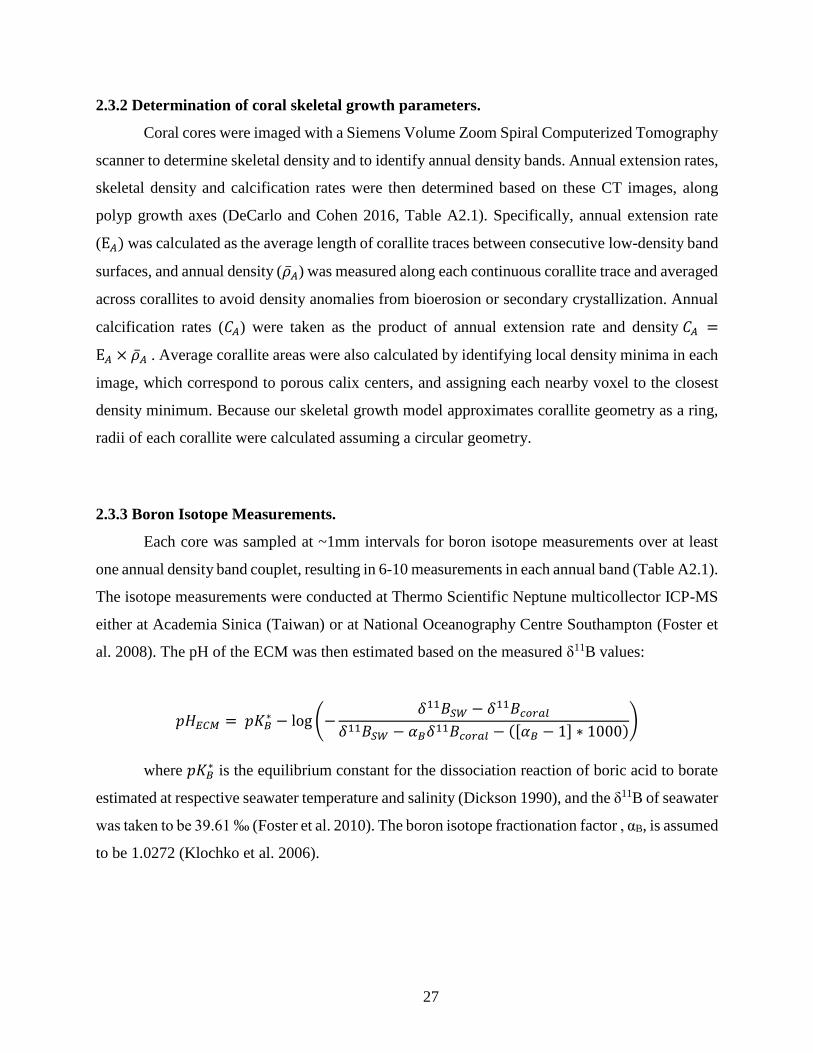
al. 2008). The pH of the ECM was then estimated based on the measured δ11B values:
𝑝𝐻𝐸𝐶𝑀 = 𝑝𝐾𝐵∗ − log (−
𝛿11𝐵𝑆𝑊 − 𝛿11𝐵𝑐𝑜𝑟𝑎𝑙
𝛿11𝐵𝑆𝑊 − 𝛼𝐵𝛿11𝐵𝑐𝑜𝑟𝑎𝑙 − ([𝛼𝐵 − 1] ∗ 1000))
where 𝑝𝐾𝐵∗ is the equilibrium constant for the dissociation reaction of boric acid to borate
estimated at respective seawater temperature and salinity (Dickson 1990), and the δ11B of seawater
was taken to be 39.61 ‰ (Foster et al. 2010). The boron isotope fractionation factor , αB, is assumed
to be 1.0272 (Klochko et al. 2006).
28
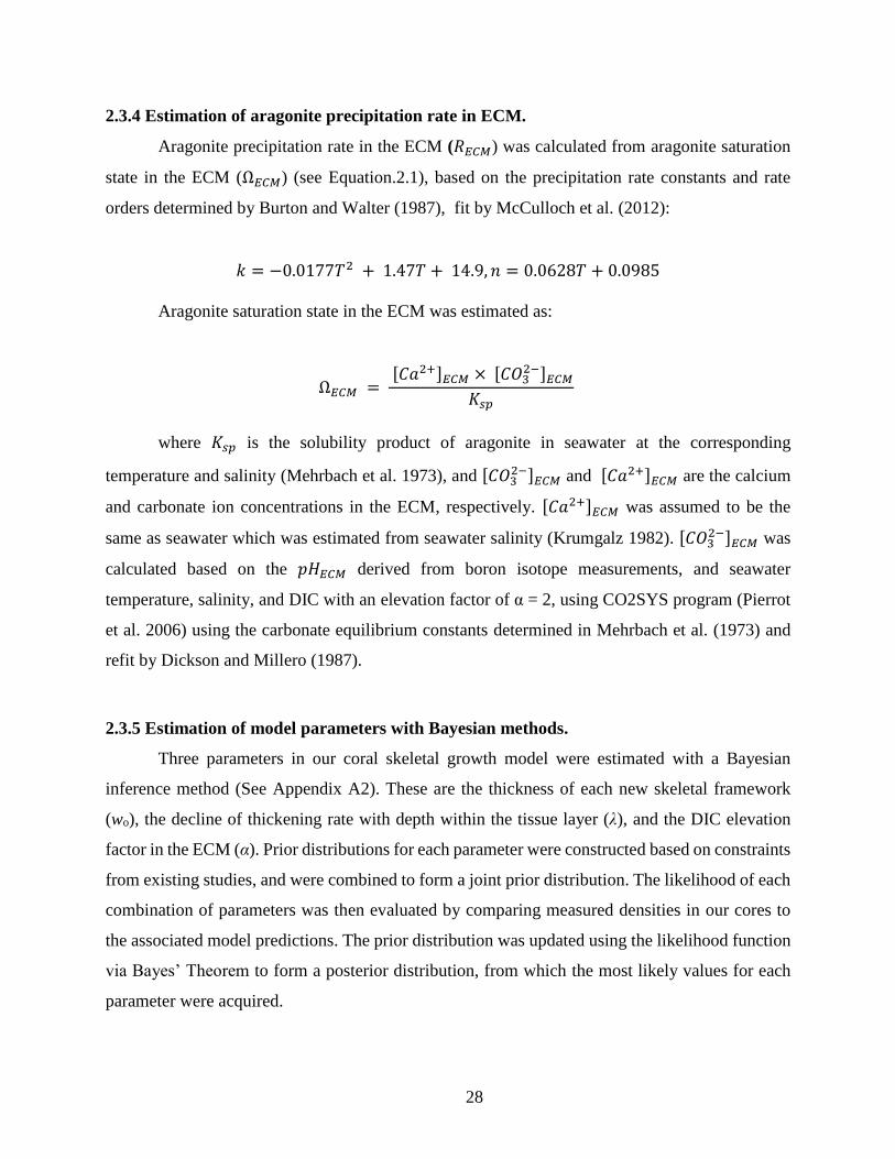
2.3.4 Estimation of aragonite precipitation rate in ECM.
Aragonite precipitation rate in the ECM (𝑅𝐸𝐶𝑀) was calculated from aragonite saturation
state in the ECM (Ω𝐸𝐶𝑀) (see Equation.2.1), based on the precipitation rate constants and rate
orders determined by Burton and Walter (1987), fit by McCulloch et al. (2012):
𝑘 = −0.0177𝑇2 + 1.47𝑇 + 14.9, 𝑛 = 0.0628𝑇 + 0.0985
Aragonite saturation state in the ECM was estimated as:
Ω𝐸𝐶𝑀 = [𝐶𝑎2+]𝐸𝐶𝑀 × [𝐶𝑂3
2−]𝐸𝐶𝑀
𝐾𝑠𝑝
where 𝐾𝑠𝑝 is the solubility product of aragonite in seawater at the corresponding
temperature and salinity (Mehrbach et al. 1973), and [𝐶𝑂32−]𝐸𝐶𝑀 and [𝐶𝑎2+]𝐸𝐶𝑀 are the calcium
and carbonate ion concentrations in the ECM, respectively. [𝐶𝑎2+]𝐸𝐶𝑀 was assumed to be the
same as seawater which was estimated from seawater salinity (Krumgalz 1982). [𝐶𝑂32−]𝐸𝐶𝑀 was
calculated based on the 𝑝𝐻𝐸𝐶𝑀 derived from boron isotope measurements, and seawater
temperature, salinity, and DIC with an elevation factor of α = 2, using CO2SYS program (Pierrot
et al. 2006) using the carbonate equilibrium constants determined in Mehrbach et al. (1973) and
refit by Dickson and Millero (1987).
2.3.5 Estimation of model parameters with Bayesian methods.
Three parameters in our coral skeletal growth model were estimated with a Bayesian
inference method (See Appendix A2). These are the thickness of each new skeletal framework
(wo), the decline of thickening rate with depth within the tissue layer (λ), and the DIC elevation
factor in the ECM (α). Prior distributions for each parameter were constructed based on constraints
from existing studies, and were combined to form a joint prior distribution. The likelihood of each
combination of parameters was then evaluated by comparing measured densities in our cores to
the associated model predictions. The prior distribution was updated using the likelihood function
via Bayes’ Theorem to form a posterior distribution, from which the most likely values for each
parameter were acquired.
29
2.3.6 Comparison of model prediction with existing studies.
Porites corals from five reefs reported in six previous studies were used to evaluate the
accuracy of our skeletal growth model in predicting coral skeletal density. These corals were
collected from reefs in the Galapagos, the Andaman Sea, the Great Barrier Reef, the Caribbean,
and the Arabian Gulf (Lough and Barnes 2000; Poulsen et al. 2006; Tanzil et al. 2009, 2013; Crook
et al. 2013; Manzello et al. 2014). Besides three parameters estimated above with Bayesian
methods, other parameters required for our model prediction include E, ro, Td, seawater
temperature, salinity and carbonate chemistry (from which 𝑅ECM is calculated). Among these, only
E was reported in all the studies. When not reported, ro and Td values were estimated from either
studies conducted at nearby reef sites or from taxonomic averages for each species (See Appendix
A2). In situ measurements of seawater carbonate chemistry, sea surface temperature and salinity,
whenever available, were used to calculate RECM; when not available, pH, DIC, salinity, and
temperature outputs from the CESM-BGC run were averaged over the time period skeletal growth
parameters were measured and used to estimate RECM. As none of these studies determined
carbonate chemistry of the coral ECM, we estimated the coral pHECM based on the pHECM ~ pHSW
correlation observed in laboratory Porites manipulation experiments (Trotter et al. 2011) which
cover a pHsw range similar to these studies (i.e. 7.19 to 8.09 v.s. 7.23 to 8.15).
2.3.7 Projection of future skeletal density changes for global reefs.
Changes in skeletal density on different reefs were predicted based on output from the
CESM-BGC RCP 8.5 21st century prediction run. Monthly projections of DIC, pH, T, and S from
the first ten (2006-2015) and last ten (2090-2099) years of the run were extracted from the 1o x 1o
model and averaged to represent the current and end of century seawater conditions at different
reef sites around the globe. Reef site locations are provided by ReefBase database of reef sites
(McManus and Ablan 1996). Skeletal growth parameters, E (annual extension rate), Td (tissue
thickness), and ro (polyp radii), were prescribed at 1.0 cm yr-1, 0.56 cm, and 0.063 cm respectively
(the average values observed in our cores), and were held constant for predictions over the 21th
century. The effect of temperature on the reaction kinetics of aragonite precipitation was not
considered in the model projection. A detailed analysis of the effects of the rising 21st century
temperature on model predictions is presented in Appendix A2.
30
2.4 Figures
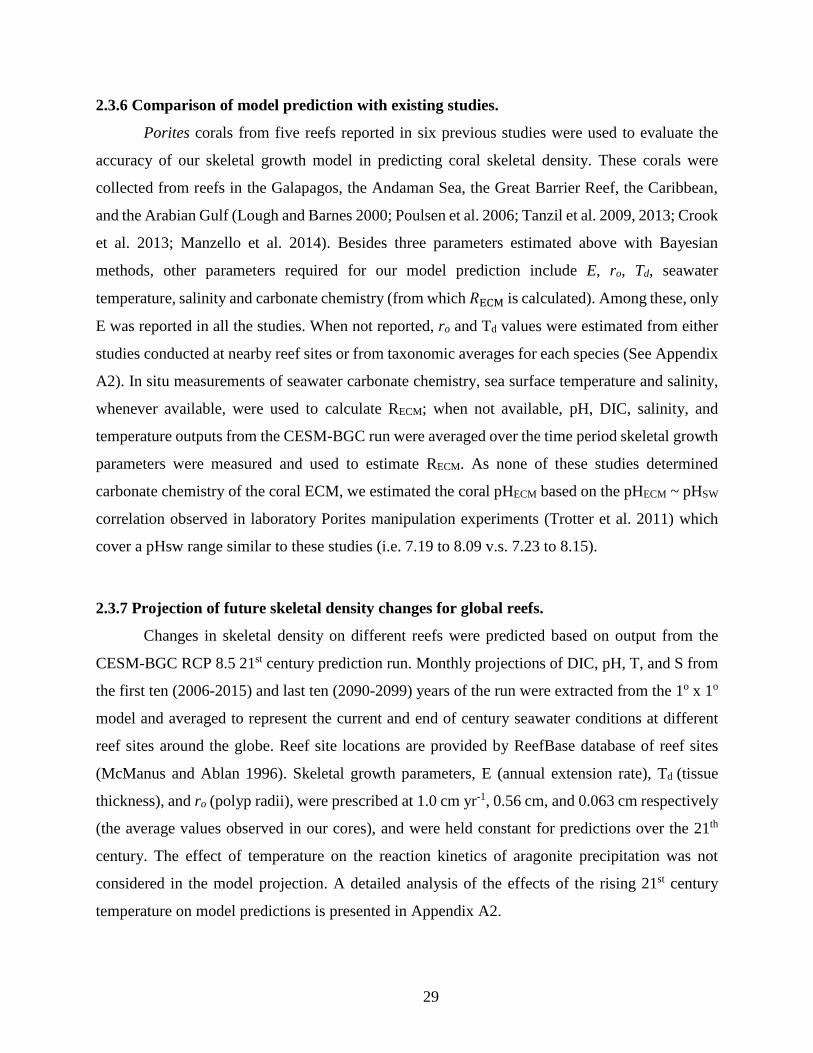
Figure 2.1. Coral skeletal parameters measured in representative Porites cores from four
reefs across the Pacific. Coral calcification rates do not correlate with either Ωsw or
ΩECM (A and B). Instead, skeletal density exhibits a significant positive correlation with both
Ωsw and ΩECM (C and D), but extension does not (E and F; P = 0.14 and P = 0.09, respectively).
Individual points represent annual averages of skeletal growth. Error bars denote 1 SD of Ω
propagated from seasonal variability in seawater physicochemical parameters (for Ωsw and ΩECM)
and in boron isotope compositions of coral skeletons (for ΩECM).
31
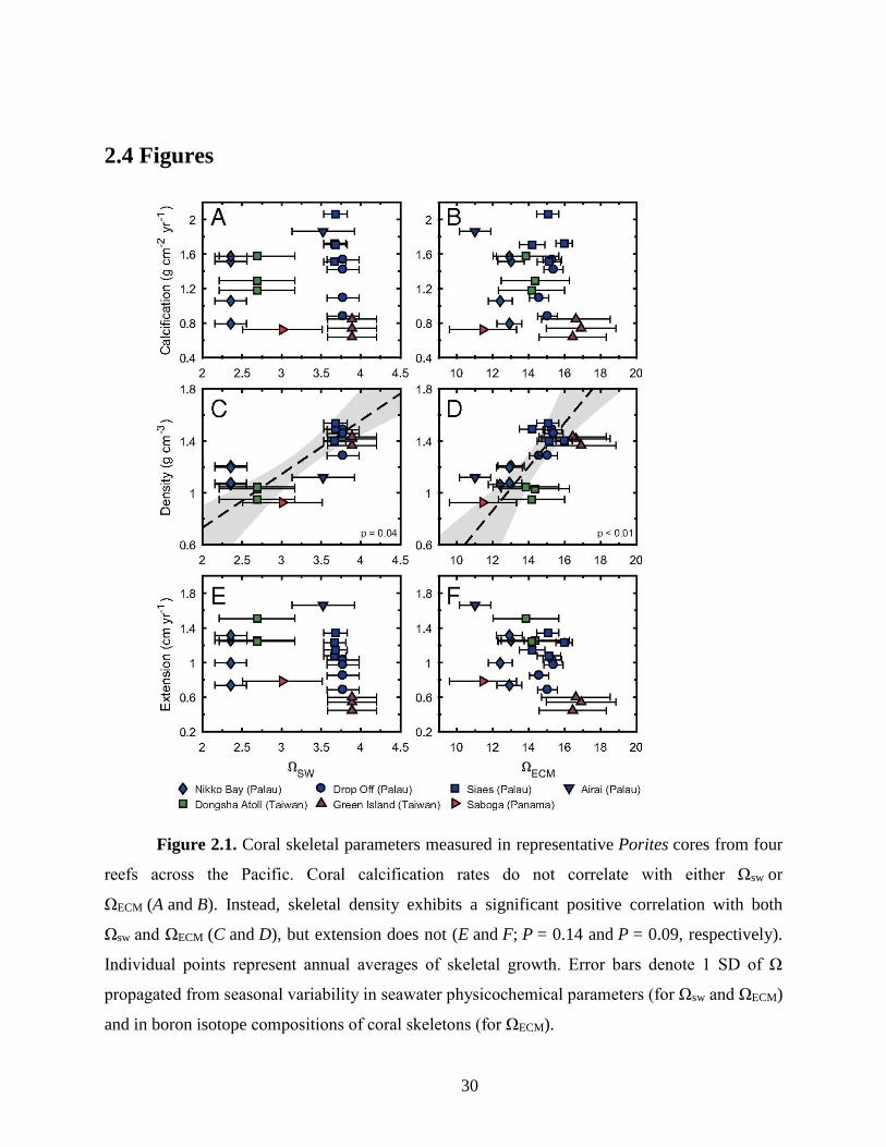
Figure 2.2. Correlation between coral skeletal density and expected aragonite precipitation
rate in the coral ECM (RECM) on both the annual (A) and seasonal (B and C) scales. Data
in A represent the same cores as in Fig. 1. Error bars (A) and shaded areas (B and C) denote 1 SD
in RECM as propagated from uncertainties in seawater parameters and in boron isotope
measurements. Seasonal density profiles were retrieved parallel to the sampling track for boron
isotope measurements.
32
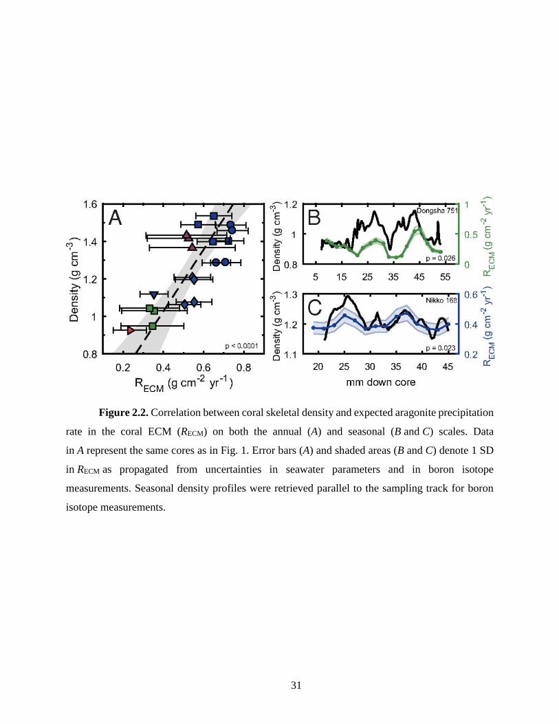
Figure 2.3. Schematic representation of our Porites skeletal growth model (A) and
comparison between model-predicted skeletal density and measured density (B). Also shown
in A are a cross-section view of our model polyp geometry and a representative SEM image of
a Porites calyx (orange dashed line). Porites cores in B were collected from reefs in the Pacific,
Atlantic, and Indian Oceans reported in previous studies (9, 30, 54–57). Data points from this
study, the Caribbean, and the Andaman Sea represent densities of individual cores; data points
from the Galapagos, the Great Barrier Reef, and the Andaman Sea represent site average densities
for which error bars denote 2σ uncertainties. Vertical error bars represent uncertainties in model
prediction propagated from uncertainties in model parameters α, λ, and wo as well as
measurements of in situ seawater conditions where available. Where seawater conditions were not
reported, outputs from the CESM-BGC historical run were adopted.
33
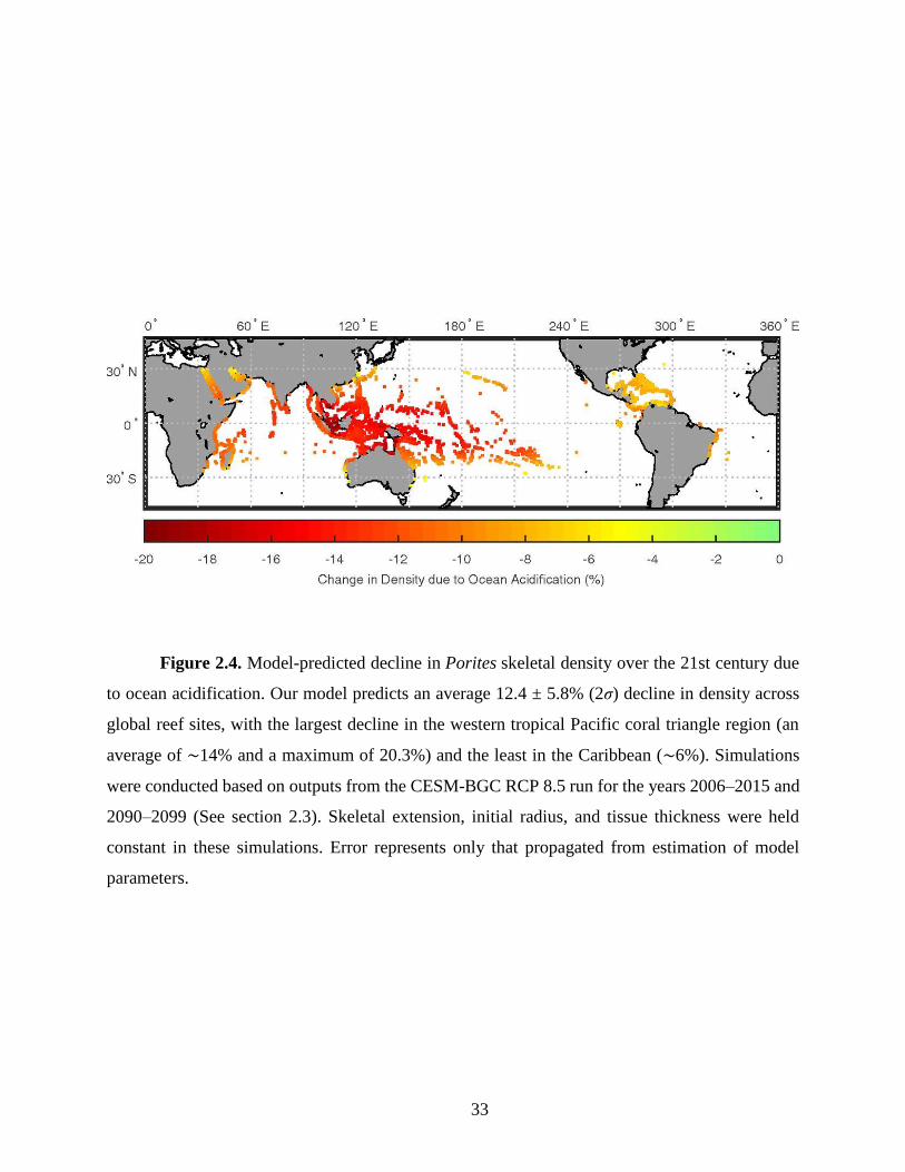
Figure 2.4. Model-predicted decline in Porites skeletal density over the 21st century due
to ocean acidification. Our model predicts an average 12.4 ± 5.8% (2σ) decline in density across
global reef sites, with the largest decline in the western tropical Pacific coral triangle region (an
average of ∼14% and a maximum of 20.3%) and the least in the Caribbean (∼6%). Simulations
were conducted based on outputs from the CESM-BGC RCP 8.5 run for the years 2006–2015 and
2090–2099 (See section 2.3). Skeletal extension, initial radius, and tissue thickness were held
constant in these simulations. Error represents only that propagated from estimation of model
parameters.
34
2.5 References
Al-Rousan S (2012) Skeletal extension rate of the reef building coral Porites species from Aqaba
and their environmental variables. Nat Sci 4:
Allemand D, Tambutte E, Girard J, Jaubert J, Tambutté E, Girard J, Jaubert J (1998) Organic
matrix synthesis in the scleractinian coral Stylophora pistillata: role in biomineralization and
potential target of the organotin tributyltin. J Exp Biol 201:2001–9
Allemand D, Tambutté É, Zoccola D, Tambutté S (2011) Coral Calcification , Cells to Reefs.
Allison N, Cohen I, Finch AA, Erez J, Tudhope AW, Facility EIM (2014) Corals concentrate
dissolved inorganic carbon to facilitate calcification. Nat Commun 5:5741
Barkley HC, Cohen AL, Golbuu Y, Starczak VR, Decarlo TM, Shamberger KEF (2015) Changes
in coral reef communities across a natural gradient in seawater pH. Sci Adv 1–7
Barnes DJ, Lough JM (1993) On the nature and causes of density banding in massive coral
skeletons. J Exp Mar Bio Ecol 167:91–108
Buddemeier RW, Maragos JE, Knutson DW (1974) Radiographic studies of reef coral
exoskeletons: Rates and patterns of coral growth. J Exp Mar Bio Ecol 14:179–199
Burton EA, Walter LM (1987) Relative precipitation rates of aragonite and Mg calcite from
seawater: temperature or carbonate ion control? Geology 15:111–114
Cai W, Ma Y, Hopkinson BM, Grottoli G, Warner ME, Ding Q, Hu X, Yuan X, Schoepf V, Xu
H, Han C, Melman TF, Hoadley KD, Pettay DT, Matsui Y, Baumann JH, Levas S, Ying Y,
Wang Y (2016) Microelectrode characterization of coral daytime interior pH and carbonate
chemistry. Nat Commun 1–8
Cantin NE, Cohen AL, Karnauskas KB, Tarrant AM, McCorkle DC (2010) Ocean Warming Slows
Coral Growth in the Central Red Sea. 329:322–325
Chan NCS, Connolly SR (2013) Sensitivity of coral calcification to ocean acidification: A meta-
analysis. Glob Chang Biol 19:282–290
Clode PL, Marshall AT (2002) Low temperature FESEM of the calcifying interface of a
scleractinian coral. Tissue Cell 34:187–198
35
Clode PL, Marshall AT (2003) Calcium associated with a fibrillar organic matrix in the
scleractinian coral Galaxea fascicularis. Protoplasma 220:153–161
Cohen AL, McConnaughey TA (2003) Geochemical Perspectives on Coral Mineralization. Rev
Mineral Geochemistry 54:151–187
Coles SL, Jokiel PL (1977) Effects of temperature on photosynthesis and respiration in hermatypic
corals. Mar Biol 43:209–216
Comeau S, Edmunds PJ, Spindel NB, Carpenter RC (2014) Fast coral reef calcifiers are more
sensitive to ocean acidification in short-term laboratory incubations. Limnol Ocean 59:1081–
1091
Constantz BR (1986) Coral Skeleton Construction : A Physiochemically Dominated Process.
Palaios 1:152–157
Cooper TF, De’ath G, Fabricius KE, Lough JM (2008) Declining coral calcification in massive
Porites in two nearshore regions of the northern Great Barrier Reef. Glob Chang Biol 14:529–
538
Crook ED, Cohen AL, Rebolledo-Vieyra M, Hernandez L, Paytan A (2013) Reduced calcification
and lack of acclimatization by coral colonies growing in areas of persistent natural
acidification. Proc Natl Acad Sci U S A 110:11044–9
Cuif JP, Dauphin YY, Doucet J, Salome M, Susini J (2003) XANES mapping of organic sulfate
in three scleractinian coral skeletons. Geochim Cosmochim Acta 67:75–83
DeCarlo TM, Cohen AL (2016) coralCT: software tool to analyze computerized tomography (CT)
scans of coral skeletal cores for calcification and bioerosion rates.
DeCarlo TM, Cohen AL (2017) Dissepiments, density bands, and signatures of thermal stress in
Porites skeletons. Coral Reefs 1–13
Dickson AG (1990) Thermodynamics of the dissociation of boric acid in synthetic seawater from
273.15 to 318.15 K. Deep Sea Res Part A, Oceanogr Res Pap 37:755–766
Dickson AG, Millero FJ (1987) A comparison of the equilibrium constants for the dissociation of
carbonic acid in seawater media. Deep Sea Res Part A, Oceanogr Res Pap 34:1733–1743
36
Doney SC, Fabry VJ, Feely RA, Kleypas JA (2009) Ocean Acidification: The Other CO2 Problem.
Ann Rev Mar Sci 1:169–192
Dustan P (1975) Growth and Form in the Reef-Building Coral Montastrea annularis. Mar Biol
33:101–107
Enochs IC, Manzello DP, Donham EM, Kolodziej G, Okano R, Johnston L, Young C, Iguel J,
Edwards CB, Fox MD, Valentino L, Johnson S, Benavente D, Clark SJ, Carlton R, Burton T,
Eynaud Y, Price NN (2015) Shift from coral to macroalgae dominance on a volcanically
acidified reef. Nat Clim Chang 5:1–9
Euw S Von, Zhang Q, Manichev V, Murali N, Gross J, Feldman LC, Gustafsson T, Flach C,
Mendelsohn R, Falkowski PG (2017) Biological control of aragonite formation in stony
corals. 938:933–938
Fabricius KE, Langdon C, Uthicke S, Humphrey C, Noonan S, De ’ath G, Okazaki R, Muehllehner
N, Glas MS, Lough JM (2011) Losers and winners in coral reefs acclimatized to elevated
carbon dioxide concentrations. Nat Clim Chang 1:165–169
Fantazzini P, Mengoli S, Pasquini L, Bortolotti V, Brizi L, Mariani M, Giosia M Di, Fermani S,
Capaccioni B, Caroselli E, Prada F, Zaccanti F, Levy O, Dubinsky Z, Kaandorp JA, Konglerd
P, Cuif J, Weaver JC, Fabricius KE, Wagermaier W, Fratzl P, Falini G, Goffredo S (2015)
Gains and losses of coral skeletal porosity changes with ocean acidification acclimation. Nat
Commun
Foster GL, Pogge Von Strandmann PAE, Rae JWB (2010) Boron and magnesium isotopic
composition of seawater. Geochemistry, Geophys Geosystems 11:1–10
Foster GL, Rae J, Elliot T (2008) Boron isotope measurements of marine carbonate using MC-
ICPMS. Geochim Cosmochim Acta 72:279
Gagan MK, Dunbar GB, Suzuki A (2012) The effect of skeletal mass accumulation in Porites on
coral Sr/Ca and ??18O paleothermometry. Paleoceanography 27:1–16
Gattuso J-P, Allemand D, Frankignoulle M (1999) Photosynthesis and Calcification at Cellular,
Organismal and Community Levels in Coral Reefs: A Review on Interactions and Control by
Carbonate Chemistry. Am Zool 39:160–183
37
Hoegh-Guldberg O, Mumby PJ, Hooten AJ, Steneck RS, Greenfield P, Gomez E, Harvell CD,
Sale PF, Edwards a J, Caldeira K, Knowlton N, Eakin CM (2007) Coral Reefs Under Rapid
Climate Change and Ocean Acidification. Science (80- ) 318:1737–1742
Hönisch B, Hemming NG, Grottoli AG, Amat A, Hanson GN, Bijma J (2004) Assessing
scleractinian corals as recorders for paleo-pH: Empirical calibration and vital effects.
Geochim Cosmochim Acta 68:3675–3685
Hooidonk R Van, Maynard J, Tamelander J, Gove J (2016) Local-scale projections of coral reef
futures and implications of the Paris Agreement. Nat Publ Gr 1–8
Kleypas J (1999) Geochemical Consequences of Increased Atmospheric Carbon Dioxide on Coral
Reefs. Science (80- ) 284:118–120
Klochko K, Kaufman AJ, Yao W, Byrne RH, Tossell JA (2006) Experimental measurement of
boron isotope fractionation in seawater. Earth Planet Sci Lett 248:261–270
Krumgalz BS (1982) Calcium distribution in the world ocean waters. Oceanol Acta 5:121–128
Langdon C, Takahashi T, Marubini F, Atkinson M, Sweeney C, Aceves H, Barnett H, Chipman
D, Goddard J (2000) Effect of calcium carbonate saturation state on the rate of calcification
of an experimental coral reef. Global Biogeochem Cycles 14(2):639–654
Van de Locht R, Verch A, Saunders M, Dissard D, Rixen T, Moya A, Kroger R (2013)
Microstructural evolution and nanoscale crystallography in scleractinian coral spherulites. J
Struct Biol 183:57–65
Lough JM (2008) Coral calcification from skeletal records revisited. Mar Ecol Prog Ser 373:257–
264
Lough JM, Barnes DJ (2000) Environmental controls on growth of the massive coral Porites. J
Exp Mar Bio Ecol 245:225–243
Lough JM, Cooper TF (2011) New insights from coral growth band studies in an era of rapid
environmental change. Earth-Science Rev 108:170–184
Madin JS, Hughes TP, Connolly SR (2012) Calcification, Storm Damage and Population
Resilience of Tabular Corals under Climate Change. PLoS One 7:1–10
38
Manzello DP, Enochs IC, Bruckner A, Renaud PG, Kolodziej G, Budd DA, Carlton R, Glynn PW
(2014) Galapagos coral reef persistence after ENSO warming across an acidification gradient.
Geophys Res Lett 41:9001–9008
McCulloch M, Falter J, Trotter J, Montagna P (2012) Coral resilience to ocean acidification and
global warming through pH up-regulation. Nat Clim Chang 2:623–627
Mcculloch MT, Olivo JPD, Falter J, Holcomb M, Trotter JA (2017) Coral calcification in a
changing World and the interactive dynamics of pH and DIC upregulation. 1–8
McManus JM, Ablan MC (1996) ReefBase: a global database on coral reefs and their resources.
Mehrbach C, Culberson CH, Hawley JE, Pytkowicz RM (1973) Measurement of the apparent
dissociation constants of carbonic acid in seawater at atmospheric pressure. Limnol Oceanogr
18:897–907
Meissner KJ, Lippmann T, Gupta A Sen (2012) Large-scale stress factors affecting coral reefs:
Open ocean sea surface temperature and surface seawater aragonite saturation over the next
400 years. Coral Reefs 31:309–319
Michael Huston (1985) Variation in coral growth rates with depth at Discovery Bay, Jamaica.
Coral Reefs 4:19–25
Northdruft LD, Webb GE (2007) Microstructure of common reef-building coral genera Acropora,
Pocillopora, Goniastrea and Porites: constraints on spatial resolution in geochemical
sampling. Facies - Carbonate Sedimentol Paleoecol 53:1–26
Pandolfi JM, Connolly SR, Marshall DJ, Cohen AL (2011) Projecting Coral Reef Futures Under
Global Warming and Ocean Acidification. Science (80- ) 333:418–422
Pierrot, Lewis DE, Wallace DWR (2006) MS Excel Program Developed for CO2 System
Calculations. ORNL/CDIAC-105a
Poulsen A, Burns K, Lough J, Brinkman D, Delean S (2006) Trace analysis of hydrocarbons in
coral cores from Saudi Arabia. Org Geochem 37:1913–1930
Reynolds RW, Smith TM, Liu C, Chelton DB, Casey KS, Schlax MG (2007) Daily high-
resolution-blended analyses for sea surface temperature. J Clim 20:5473–5496
39
Sammarco P, Risk M (1990) Large-scale patterns in internal bioerosion of Porites: cross
continental shelf trends on the Great Barrier Reef. Mar Ecol Prog Ser 59:145–156
Shirai K, Sowa K, Watanabe T, Sano Y, Nakamura T, Clode P (2012) Visualization of sub-daily
skeletal growth patterns in massive Porites corals grown in Sr-enriched seawater. J Struct
Biol 180:47–56
Sorauf J (1970) Microstructure and formation of dissepiments in the skeleton of the recent
scleractinia (hexacorals). Biomineralization 2:1–22
Stolarski J (2003) Three-dimensional micro- and nanostructural characteristics of the scleractinian
coral skeleton: A biocalcification proxy. Acta Palaeontol Pol 48:497–530
Tambutté E, Venn AA, Holcomb M, Segonds N, Techer N, Zoccola D, Allemand D, Tambutté S
(2015) Morphological plasticity of the coral skeleton under CO2-driven seawater
acidification. Nat Commun 6:7368
Tambutté S, Holcomb M, Ferrier-Pagès C, Reynaud S, Tambutté E, Zoccola D, Allemand D
(2011) Coral biomineralization: From the gene to the environment. J Exp Mar Bio Ecol
408:58–78
Tambutté S, Tambutté E, Zoccola D, Caminiti N, Lotto S, Moya A, Allemand D, Adkins J (2007)
Characterization and role of carbonic anhydrase in the calcification process of the
azooxanthellate coral Tubastrea aurea. Mar Biol 151:71–83
Tanzil JTI, Brown BE, Dunne RP, Lee JN, Kaandorp JA, Todd PA (2013) Regional decline in
growth rates of massive Porites corals in Southeast Asia. Glob Chang Biol 19:3011–3023
Tanzil JTI, Brown BE, Tudhope AW, Dunne RP (2009) Decline in skeletal growth of the coral
Porites lutea from the Andaman Sea, South Thailand between 1984 and 2005. Coral Reefs
28:519–528
Taylor RB, Barnes DJ, Lough JM (1993) Simple-Models of Density Band Formation in Massive
Corals. J Exp Mar Bio Ecol 167:109–125
Tomascik T, Sander F (1985) Effects of eutrophication on reef-building corals. Mar Biol 87:143–
155
40
Trotter J, Montagna P, McCulloch M, Silenzi S, Reynaud S, Mortimer G, Martin S, Ferrier-Pagès
C, Gattuso J-P, Rodolfo-Metalpa R (2011) Quantifying the pH “vital effect” in the temperate
zooxanthellate coral Cladocora caespitosa: Validation of the boron seawater pH proxy. Earth
Planet Sci Lett 303:163–173
Venn A, Tambutté E, Holcomb M, Allemand D, Tambutté S (2011) Live tissue imaging shows
reef corals elevate pH under their calcifying tissue relative to seawater. PLoS One 6:
Warner ME, Fitt WK, Schmidt GW (1996) The effects of elevated temperature on the
photosynthetic efficiency of zooxanthellae in hospite from four different species of reef coral:
a novel approach. Plant Cell Environ 19:291–299
Watanabe T, Fukuda I, Katsunori C, Yeisin I (2003) Molecular analyses of protein components of
the organic matrix in the exoskeleton of two scleractinian coral species. Comp Biochem
Physiol Part B Biochem Mol Biol 136:767–774
Wells JW (1956) Scleractinia. Treatise on invertebrate paleontology F. Coelenterata. Geological
Society of America & University of Kansas Press, pp 328–440
Woesik R Van, Woesik K Van, Woesik L Van (2013) Effects of ocean acidification on the
dissolution rates of reef-coral skeletons. PeerJ 1–15
41
Chapter 3 – Skeletal records of bleaching
reveal different thermal thresholds of
Pacific coral reef assemblages
Nathaniel R. Mollica, Anne L. Cohen, Alice Alpert, Hannah C. Barkley, Russell E. Brainard,
Jessica Carilli, Thomas M. DeCarlo, Elizabeth Drenkard, George Lohmann, Sangeeta
Mangubhai, Kathryn Pietro, Hanny E. Rivera, Randi D. Rotjan, Celina Scott-Beuchler, Andrew
Solow, and Charles Young
Published in Coral Reefs, May 2nd, 2019
3.1 Introduction
Reef-building corals exist in an obligate symbiosis with single celled dinoflagellates called
zooxanthellae, which provide a significant component of the host energetic needs. When sea
surface temperatures (SSTs) exceed a physiological threshold, the relationship between corals and
zooxanthellae breaks down, the symbionts are expelled, and the coral loses pigmentation in a
process called “bleaching” (e.g. Coles and Jokiel 1977). Prolonged or severe bleaching can lead to
coral starvation and, eventually, death. Coral bleaching was first reported in 1963 (Donner et al.
2017), and regional-scale or mass bleaching of coral communities and reefs was first reported
during the 1982/3 super El Niño (Hoegh-Guldberg and Smith 1989). As the oceans continued to
warm over the subsequent three decades, episodes of mass bleaching increased in frequency and
extent, and now occur with each El strong Niño (Hughes et al. 2018). By 2008, bleaching had
caused irretrievable loss of an estimated 19% of reef area worldwide (Wilkinson 2008), and losses
following the recent 2015-2016 El Niño are expected to exceed this estimate. As global
temperatures rise, by a projected 1 to 2.5 °C over this century, (IPCC AR5 2014) there is mounting
concern that coral communities will soon experience bleaching at a frequency from which they
cannot recover.
Significant effort is currently invested in identifying coral reef ecosystems or communities
that might survive ocean warming (Pratchett et al. 2008; Frieler et al. 2012; van Hooidonk et al.
2016; Beyer et al. 2018). These efforts are limited in large part, however, by two unknowns. First,
42
the spatial resolution of general circulation models (GCMs) is too coarse to resolve reef-scale
hydrodynamics, meaning projections of future open ocean conditions may not apply to many
shallow water reef systems. Statistical and dynamical downscaling of GCM output is one approach
taken to specifically addressing this issue (Donner 2009; Frieler et al. 2012; van Hooidonk et al.
2016). Second, the thermal thresholds for bleaching of different reef systems are not well
characterized. Currently, a single bleaching threshold based on 1C warmer than the maximum
monthly mean (MMM) SST is used to predict whether, and with what severity, bleaching will
occur during heatwaves and in model projections of future global change scenarios (Heron et al.
2015). However, thermal thresholds differ amongst species (e.g. Coles and Jokiel 1977), amongst
coral communities within and between reefs (e.g., Fisk and Done 1985; Rowan et al. 1997; Van
Woesik et al. 2011) and examples exist of thermal thesholds changing over time (Maynard et al.
2008). While a few studies have incorporated inter-reef differences in thermal tolerance (van
Hooidonk and Huber 2009; Donner 2011) and the potential for coral acclimatization (e.g. Logan
et al. 2014) into projections of coral reef futures, these have been limited in assigning site-specific
thermal thresholds by the paucity of observational bleaching records (van Hooidonk and Huber
2009).
This study addresses the second issue, i.e. the lack of constraint on coral thermal thresholds.
Bleaching histories for reef locations around the globe have been compiled (e.g. Donner et al.
2017; Hughes et al. 2018), but all are limited by the paucity of observational data, especially but
not limited to, remote reef locations. Here, we make a start at filling spatial and temporal gaps in
bleaching records using signatures of bleaching archived in the skeletons of massive long-lived
corals that survived, and recorded, multiple bleaching events extending back in time (Fig. 3.1).
Skeletal “stress bands” have been linked, qualitatively, with anomalously high summertime SSTs
and coral bleaching (Smithers and Woodroffe 2001; Hendy et al. 2003; Cantin et al. 2010; Carilli
et al. 2010, 2012; Cantin and Lough 2014; Mallela et al. 2015). Recently, Barkley and Cohen
(2016) and Barkley et al., (2018) demonstrated a statistically significant relationship between the
prevalence of stress bands in massive Porites spp. corals and the severity of observed bleaching in
the coral community on multiple reefs within the Palau archipelago, and on Howland and Jarvis
Islands in the CEP. These observations support the utility of skeletal stress bands as proxies for
historical bleaching severity in the absence of observational data.
43
In this study, we first build on the original calibration of bleaching incidence within a coral
community (hereafter ‘observed bleaching incidence’) against the prevalence of stress bands in
massive coral skeletons (hereafter ‘stress band prevalence’) (Barkley et al. 2018) by including new
data from the Pacific and the Caribbean (Fig. 3.2). The new calibration includes 11 reef systems,
multiple massive coral genera and represents multiple coral community compositions. Second, we
apply the calibration to stress band records constructed from 8 central Pacific reef systems,
spanning the time period 1982-2015. Third, we refine the NOAA thermal stress index (Degree
Heating Weeks, DHW) calculation to enable estimates of thermal stress in the CEP, where SST
variability on inter-annual timescales is dominant. We use a percentile-based method, independent
of seasonality, to calculate the DHWs and cumulative thermal stress (Total Hotspot) for each
heatwave at each site over the corresponding time period 1982-2015. We then compare the severity
of the bleaching response to the level of thermal stress imposed on each reef during each event and
construct reef-specific thermal sensitivity curves and a thermal tolerance index (b½) for each reef
system. Finally, we assess the thermal tolerance indices against multiple physiological and
climatological factors to evaluate the potential mechanisms underpinning the different thermal
tolerances exhibited by different reefs.
3.2 Materials and Methods
3.2.1 Collection of coral cores and identification of stress bands
247 skeletal cores were collected and analyzed from colonies of three massive coral genera
(Porites spp., Orbicella spp. and Siderastrea siderea) on eleven coral reefs in the Pacific Ocean
and Caribbean. A subset of data from each core, specifically those years for which observational
bleaching data exist, was used in the calibration. These cores are listed in Table A3.2. 122 Porites
cores were then used to construct thermal histories for the eight Pacific reefs back to 1982, and
generate the thermal sensitivity curves. These cores are listed in Table A3.3.
All cores were collected and analyzed using the same methods. Only live colonies were
cored, establishing the top age, vertically i.e., parallel to the upward growth axis, and using either
a pneumatic drill fitted with 3-cm diameter diamond tip coring bit or an hydraulic drill fitted with
an 8-cm diameter bit. Core holes were sealed with a cement cap and underwater epoxy, secured
flush with the colony surface to facilitate overgrowth of tissue and wound closure (e.g. Matson
2011), a 6 to 36-month process depending on the rate of coral growth and diameter of core. All
44
cores were first air dried in the field, then oven dried at 60 C, and CT scanned intact, together
with density standards, on the Siemens Volume Zoom Helical Computerized Tomography (CT)
Scanner at Woods Hole Oceanographic Institution or the Siemens Biograph mCT scanner at the
Biomedical Research Imaging Center (BRIC) at the University of North Carolina (protocol as per
Barkley et al. 2015; DeCarlo et al. 2015).
Stress bands and annual growth bands were identified in the CT scan images of each core
and quantified using the automated code coralCT for MATLAB which traces the density of
individual corallites within the 3 dimensional core (DeCarlo and Cohen 2016). Revisions to
version 1.1 of coralCT, which was designed primarily for Porites spp., were made to accommodate
the skeletal architecture of the Atlantic corals which have more prominent thecal walls than
Porites. Specifically, a linear quadratic estimation algorithm (i.e. Kalman Filtering) improved
polyp tracing along the core axis. The code was also revised to enable automated identification of
stress bands (Barkley et al. 2018). Specifically, the density time-series for all corallites in the core
(see DeCarlo et al. 2015, Data Repository Figure DR2) were averaged to create an "ensemble"
mean density time series for all traceable corallites. The averaged density profile time-series was
then detrended to account for shifts in mean density that may occur over time. Regions where
skeletal density exceeded 2 standard deviations above the whole-core mean, a threshold chosen to
account for the range in natural seasonal and inter-annual density variability, were identified as
stress bands (Fig. 3.1C). To exclude fine-scale density anomalies such as worm borings, stress
bands were defined as having a minimum width of 1 mm. Each CT scan was visually inspected to
validate the presence and location of stress bands identified by the automated program.
The age model for each core was developed using annual growth bands also identified in
the CT images. In corals with clear annual banding, the age model was constructed by counting
the bands from the top of the core. Where banding was unclear or ambiguous, the band-based age
model was validated using dissepiments. Specifically, the distance between successive monthly
dissepiments was quantified from photographs taken under a dissecting microscope (Fig. A3.2).
The estimate of annual extension derived from dissepiments was used to confirm the estimate
derived from annual bands, following DeCarlo and Cohen (2017) (i.e. 12.4 dissepiments per year).
The thickness of the tissue in each core used in the bleaching history reconstruction was
measured as an index of biomass or energetic reserve. The vertical distance between the top of the
45
core and the topmost dissepiment upon which the base of the tissue rests (e.g. Barnes and Lough
1992) was measured on a cut slab using a Nikon SMZ1500 stereomicroscope and SPOT imaging
software (e.g. Barkley et al. 2018).
3.2.2 Bleaching Survey Data
Published bleaching accounts were used to calibrate the proportion of skeletal stress bands
per event identified in the suite of cores against the observed bleaching incidence (represented by
the percent coral cover observed to be bleached) recorded during that event (Table A3.4). In all
cases, with the exception of the Phoenix Islands surveys in 2015 (Kanton, Rawaki, Enderbury,
Nikumaroro), bleaching was observed during or after the peak SST anomaly obtained during each
event. In the Phoenix Islands, ecological surveys and skeletal cores were obtained two months
prior to the peak SST anomaly, and it is likely that the full extent of bleaching in 2015-16 was not
captured by those surveys. However, since coring and surveys were conducted simultaneously, we
expect the stress bands to track the severity of bleaching at the time, and we used this information
in the calibration.
On Dongsha Atoll and Jarvis Island, bleaching estimates were obtained from photographic
surveys conducted in June 2015 (DeCarlo et al. 2017) and November 2015 (Barkley et al. 2018)
respectively. On Jarvis and Howland Islands in 2010, bleaching severity was assessed from Rapid
Ecological Assesments (REA) and towed-diver surveys (Vargas-Ángel et al. 2011). In the Phoenix
Islands (Kanton, Rawaki, Enderbury, and Nikumaroro) in 2015, bleaching information was
estimated from photographic surveys (Mangubhai et al. 2015; Table A3.4). In the Caribbean, coral
bleaching observations on Martinique, Barbados and Curacao in 1998, 2005 and 2010 were used
in the calibration (Wilkinson 2008; Eakin et al. 2010; Estep et al. 2017). Results were reported as
percent coral cover bleached, (Jarvis, Howland, Dongsha, and the Caribbean sites), or percent
colony bleached (Phoenix Islands). We standardized the data as follows:
𝑂𝑏𝑠𝑒𝑟𝑣𝑒𝑑 𝐵𝑙𝑒𝑎𝑐ℎ𝑖𝑛𝑔 𝐼𝑛𝑐𝑖𝑑𝑒𝑛𝑐𝑒 (%) = 𝑏𝑙𝑒𝑎𝑐ℎ𝑒𝑑 𝑐𝑜𝑟𝑎𝑙 (𝑚2)
𝑡𝑜𝑡𝑎𝑙 𝑐𝑜𝑟𝑎𝑙 (𝑚2) (3.1)
3.2.3 Sea surface temperature data and data products
We used daily satellite SSTs (November 1981 ‒ December 2016) from the AVHRR
Pathfinder Version 5.3, 4-km dataset (nighttime only) (Casey et al. 2010). For reefs from which
46
cores were collected across multiple cells, the grid cells were averaged. Average weekly SSTs
were calculated and temporal gaps in the Pathfinder data filled with mean-adjusted values from
the IGOSS OIv2 1° x 1° resolution dataset (Reynolds et al. 2002). In situ temperature loggers
deployed at Jarvis by Barkley et al., (2018), as well as our loggers deployed at Kanton, Enderbury,
Nikumaroro, and Rawaki from June 2012 to September 2015 were used to validate satellite-
derived SSTs for these central Pacific sites (Fig. A3.3). Average in situ temperatures were within
±0.25C of satellite SSTs, with two exceptions. First, on the west side of Jarvis Island, upwelling
of the Pacific Equatorial Undercurrent (EUC) lowers local temperatures relative to the east side of
the island and satellite-derived SSTs, which consistently capture east side SSTs (Alpert et al.
2016). However, during El Niño, weakening of the EUC occurs, upwelling is diminished or
entirely absent, and temperatures are homogenous around the island. Thus, during bleaching
events, temperatures on Jarvis’ west side are consistent with satellite-derived SSTs (Barkley et al.
2018). Second, in Kanton Lagoon, loggers deployed during the 2015 El Niño revealed that
daytime temperatures in the lagoon consistently exceeded both satellite-derived SSTs and logged
outer reef SSTs by up to 1C. Kanton lagoon cores were used in the calibration because bleaching
severity in the lagoon was recorded in 2015 at the same time the cores were collected. However,
we did not include lagoon cores in the down-core historical bleaching reconstruction to evaluate
thermal sensitivity because we could not constrain historical lagoon SST back to 1982 from the
satellite data.
3.2.4 Estimation of the error on the calibration of stress band proportion against observed
bleaching
The presence of a stress band in a single core during a known thermal stress event indicates
that bleaching occurred, and stress bands have been used as a binary indicator of historical
bleaching (e.g. Smithers and Woodroffe 2001; Carilli et al. 2010). Here we use stress bands to
determine when bleaching occurred and quantify its severity. However, significant uncertainty
exists in estimating the proportion of Porites spp. stress bands in the population based on cores
extracted from a relatively small fraction of the population. Further, because bleaching is variable
even on small spatial scales within a reef, there are non-trivial uncertainties associated with both
the stress band proportion and the observed bleaching incidence. To best account for these
uncertainties in calibrating the proxy, we used the Mantel-Haenszel estimator of the common odds
ratio, (Mantel and Haenszel 1959) (see Appendix A3 for detailed methods). To use the odds
47
ratio to predict bleaching incidence, a functional estimate of bleaching incidence was constructed
by inverting the odds ratio:
𝑝𝑏𝑖 = (1 +1−𝑝𝑠𝑏
𝑝𝑠𝑏)
−1
(3.2)
Where 𝑝𝑏𝑖 is the proportion of reef community bleached and 𝑝𝑠𝑏 is the proportion of stress
bands (sb) observed. From the variance in both 𝑝𝑠𝑏 and The associated variance of the prediction
was calculated as follows:
𝑉𝑎𝑟 𝑝𝑏𝑖 ≅ (𝜕𝑝𝑏𝑖
𝜕𝑝𝑠𝑏)
2
𝑉𝑎𝑟 𝑝𝑠𝑏 + (𝜕𝑝𝑏𝑖
𝜕)
2
𝑉𝑎𝑟 (3.3)
We use the variance on the predicted bleaching incidence ( 𝑉𝑎𝑟 𝑝𝑏𝑖) to define a 2σ
confidence interval for reconstructed bleaching incidence levels. The width of this confidence
interval depends therefore on three things: the number of cores collected, the prevalence of stress
bands among those cores, and the effectiveness of the common odds ratio at explaining the
calibration data (or the quality of the fit).
3.2.5 Development and application of a percentile-based estimate of thermal stress
The NOAA Coral Reef Watch Degree Heating Week (DHW) index uses the amplitude and
duration of the SST anomaly to estimate levels of thermal stress experienced by corals (Gleeson
and Strong 1995) and assumes that thermally stressful conditions occur when temperatures exceed
1C above the maximum monthly mean SST (MMM) to which corals are normally exposed.
However, in the CEP, the SST regime is dominated by inter-annual variability rather than regular
seasonal cycles and consequently the maximum temperature to which corals are normally exposed
does not occur during the same month every year. This means that the MMM does not effectively
describe the ‘upper end’ of temperatures in the CEP or other regions where seasonal variability is
not dominant. The traditional DHW metric therefore, consistently overestimates the level of
thermal stress in such regions.
To address this issue, we developed a percentile-based bleaching threshold which is
independent of the timescale of SST variability and can be applied in any oceanographic
environment. First, we calculated gap-filled Pathfinder SSTs from 1982-2016 for each grid cell
containing the reef locations represented in the global bleaching database of Donner et al., (2017).
48
To establish the maximum heat to which corals are exposed during “normal” or non-extreme years,
SSTs during ENSO neutral years between 1982 and 2012 (i.e., 1985-6, 1990, 1993-6, 2001, 2003-
6, 2012 based on years when -1.25 < Nino 3.4 < 1.25 (Trenberth 1997)) were extracted and the
site-specific distribution of weekly SSTs evaluated. A threshold percentile (e.g., 94th, 95th, 96th)
was chosen to represent the high end of SSTs typically experienced by each coral community, and
the SST value corresponding to that percentile at that site was substituted for the MMM +1C
threshold. We used the new threshold to calculate DHWs at each site. We repeated the exercise
with different percentiles and compared the resulting DHWs to the observed bleaching levels at
each site during bleaching years (Donner et al. 2017). The quality of each set of predictions was
evaluated using the Gilbert Skill Score (or Equitable Threat Score, ETS) which maximizes
predictive power while accounting for the increase in type 2 errors associated with lower
thresholds (Fig. A3.1). A percentile of 94.4th resulted in the maximum ETS (0.68 on a scale of 0
to 1, see Appendix A3). It is important to note that this method is calibrated to maximize the
predictive power of the 4 DHW alert level, and other commonly used alert levels (e.g. alert level
2 (8 DHW), under which mortality is likely) have not been at this time estimated (Liu et al. 2006).
3.2.6 Total Hotspot as an index of Cumulative Thermal Stress
The DHW Index was developed as a 3-month running forecasting metric to predict where
bleaching is likely to occur. In this study, we compare the level of thermal stress experienced by
the reef during each event, with the resulting bleaching severity. Thus, rather than DHW, we use
the Total Hotspot (TH), which is the total number of weeks during which the site-specific thermal
threshold is exceeded (Gleeson and Strong 1995). TH is calculated using the percentile-based
threshold of 94.4th instead of the traditional MMM +1 threshold as follows:
𝑇𝐻𝑒 = ∑ 𝐻𝑤𝑛𝑤=1 (3.4)
Where TH is the Total Hotspot, for event e from the first week (w = 1) to the last week (n)
during which SST exceeded the bleaching threshold. We use the TH index below to assess the
sensitivity of each coral community to thermal stress.
49
3.3 Results
3.3.1 Stress band – bleaching calibration
Stress bands were identified in the majority of cores (with the notable exception of
Kingman Reef), and only occurred in years in which SSTs were anomalously warm and TH
exceeded zero (Table A3.4, Table A3.5). No stress bands occurred in years during which thermal
stress was zero. For sites and years in which observational bleaching data are available, we
regressed the proportion of stress bands against the observed severity of coral bleaching incidence
at the same site during the same year. (Fig. 3.3). Stress bands are highly correlated with bleaching
severity (r2 = 0.945, p = 3.67e-12), consistent with Barkley and Cohen (2016) for Palau, and
Barkley et al., (2018). The common odds ratio regression, used to estimate the error on the
relationship between bleaching severity and stress band proportions (Methods, Eq. 3.2), was ψ =
1.11 ± 0.10 (2σ), implying a near 1 to 1 relationship (Fig. 3.3). We use this regression to predict
bleaching levels at sites and during times where no observations were made. The error on these
predictions is calculated using Equation 3.3 (methods) using the variance in the common odds
ratio (ψ), the number of cores sampled, and the fraction of cores that exhibit stress bands. For a
sample size of 15 cores, the maximum uncertainty on the estimate of bleaching severity is 28.7%
(2σ), which occurs at a stress band proportion of 48.3% (Fig. 3.3 shaded region).
3.3.2 Thermal Stress Indices
In Figure 3.4, DHW and TH calculated using the traditional threshold method (i.e. 1 C
above the MMM, A-I) are compared with DHW calculated using the 94.4th percentile-based (J-Q)
threshold for our study sites. In addition, we provide DHW and TH estimates for the northern
Great Barrier Reef (GBR; 10.8 S and 142.9 E) (I and R), to highlight both the different levels
and histories of thermal stress experienced by reefs in the CEP versus reefs in regions dominated
by seasonal SST variability, and the relative change in estimated severity when the percentile-
based method is applied. DHW events coincide with El Niño years at all CEP sites and their
magnitude linked to size and type of El Niño event i.e., central vs. eastern Pacific El Niño (Ashok
et al. 2007). Eastern Pacific events are felt most strongly at Jarvis (~160º W), whereas central
Pacific events are felt most strongly in the Phoenix Islands. Further west, Maiana Island, is
unaffected by eastern Pacific events instead experiencing its major thermal stress events in weak
El Niño years (e.g. 2004).
50
At all our study locations the percentile-based bleaching threshold was higher than the
MMM+1, causing lower DHW and TH estimates for each event relative to the traditional
calculation. At equatorial sites, average DHW and TH for most events were substantially different.
For example, DHWs derived by the percentile method was lower by an average of 6.3C wk and
5.8C wk at Jarvis and Kanton respectively, versus 4.5C wk and 2.3C wk for Dongsha and the
GBR. TH decreased by 10.01 and 4.1C, versus 2.14 and 0.88C at the same sites. These results
indicate that the traditional MMM+1 method overestimates thermal stress on central Pacific coral
reefs relative to other reefs (confirming the bias observed by others, e.g. Donner 2011; Lough et
al. 2018), and that the percentile method provides a non-biased method for all sites.
3.3.3 Reconstructed bleaching histories
We applied the stress band prevalence – observed bleaching incidence calibration (Fig.
3.3) to reconstruct the history and severity of bleaching at our eight central Pacific reef sites since
1982 (Fig. 3.5, Table A3.6). The young end of the reconstruction on each reef is determined by
the date the most recent cores were collected (for example 2010 on Kingman, 2016 on Jarvis, 2012
on Howland and Maiana, see Table A3.3). We do not attempt to reconstruct bleaching in the
Phoenix Islands in 2015 because the cores were retrieved two months prior to the peak SST, and
thus may not capture the full severity of the bleaching that occurred there in 2015. Stress band
counts at Jarvis Island back to 1960 are published elsewhere (Barkley et al. 2018).
Bleaching has been directly observed in the Phoenix Islands only in 2015, on Howland
Island only in 2010, and no bleaching observations have been made on Maiana or Kingman,
meaning our reconstructions significantly extend the bleaching database for this region across
space and back in time. For all reefs, excluding Kingman, our analysis reveals a history of
bleaching events, each occurring in response to El Nino-induced thermal stress. Cores collected
on Kingman Reef in 2010 and 2012 revealed no stress bands, consistent with the absence of
appreciable thermal stress (DHW > 4) over this time period (Fig. A3.4), and implying that
Kingman Reef has never experienced significant bleaching.
3.3.4 Assessment of the thermal sensitivity of coral communities
Using the reconstructed bleaching histories (Fig. 3.5, Table A3.6) and the calculated
thermal stress experienced by each reef during each bleaching event, we characterized the
sensitivity of the coral community response to thermal stress (Fig. 3.6). For each site, the
51
relationship between thermal stress and bleaching severity follows a predictable, non-linear
pattern. Because the bleaching thresholds of individual coral colonies on each reef are assumed to
be normally distributed, we used a cumulative density function (CDF) to fit the data. A minimum
amount of thermal stress is required to induce bleaching, therefore we used a lognormal CDF for
the regression:
𝐵𝐼𝑗 =100
𝜎√2𝜋 ∫
𝑒−(ln(𝑡)−µ𝑖)2/(2𝜎𝑖2)
𝑡𝑑𝑡
𝑇𝐻𝑗
0
where BIj is coral bleaching incidence at a given Total Hotspot THj and µ𝑖 and 𝜎𝑖 are
regression parameters corresponding to mean and standard deviation of the associated normal
distribution for each reef i. Data from Kanton, Rawaki, and Enderbury were pooled as the
relationship between BI and TH was not significantly different between these reefs. For the
purpose of this analysis, we excluded reconstructed BI events with greater than 35% error.
A single parameter index of the mean thermal tolerance of corals at each reef was estimated
by converting µ𝑖 to the half-point of each regression (i.e. the TH at which 50% bleaching is
predicted) as follows:
𝑏½ = 𝑒µ𝑖
Using b½ as an index of thermal tolerance implies that Jarvis Island coral communities have
the highest thermal tolerance (b½ = 29.71 ± 1.06 SE), followed by the northern Phoenix Islands
(Kanton/Enderbury/Rawaki) and that tolerances decrease westward, with Maiana Island exhibiting
the lowest thermal tolerance index (b½ = 3.04 ± 1.36 SE) of the CEP reefs studied here. We also
compare the bleaching sensitivity of these CEP reefs to the GBR using spatial (Hughes et al. 2017)
and temporal (Donner et al. 2017) bleaching observations versus percentile based TH estimates.
The GBR data help to put the thermal tolerances of the central Pacific reefs in perspective,
exhibiting an even lower thermal tolerance index than Maiana (b½ =1.03 ± 1.04 SE).
3.4 Discussion
The occurrence of mass coral reef bleaching events associated with ocean warming has
motivated efforts to better predict coral reef futures (Pandolfi et al. 2011). While some efforts are
based predominantly on GCM projections of temperature (Beyer et al. 2018), others are
52
incorporating variable and potentially shifting thermal thresholds, as observed in nature (Coles and
Jokiel 1977; Fisk and Done 1985; Rowan et al. 1997; Maynard et al. 2008; Van Woesik et al. 2012;
Hughes et al. 2017). Nevertheless, characterizing the thermal tolerances of different reef
communities and evaluating change over time are difficult because they require direct, repeat
observations of coral communities during periods of thermal stress. Here we used skeletal stress
bands to fill gaps in observational bleaching data on eight central Pacific coral reef islands since
1982. Our study builds on pioneering work by Emiliani et al. (1978) who identified stress bands
in a Montastrea coral (now Orbicella), and by Hudson et al. (1976) who attributed anomalously
high density bands in the same species to environmental stress. Subsequent work by Cantin and
Lough (2014) construct bleaching histories from the GBR, and Carilli et al., (2009) used stress
bands to evaluate effects of local stressors on bleaching incidence in the Caribbean and
subsequently Barkley and Cohen (2016) showed that the proportion of stress bands reflected the
severity of bleaching in the coral reef community. These observations paved the way for the use
of skeletal records to provide quantitative information about reef responses to thermal stress in the
absence of direct observations (DeCarlo et al. 2017; Barkley et al. 2018).
3.4.1 The stress band-bleaching relationship and a conceptual model of the mechanism
We expanded the original calibration of Barkley and Cohen (2016) using new
observational bleaching data and measurements of stress band prevalence in three massive coral
genera in the Pacific and Caribbean These results show that the relationship applies beyond just
Pacific reefs and Pacific Porites corals, and leads naturally to the question: why is the prevalence
of stress bands in massive corals so well correlated with the incidence of bleaching across the
community of mixed coral taxa? We propose that within each population of massive corals, a range
of thermal thresholds exist (Fig. 3.6B). When thermal stress is low, only the most sensitive massive
corals in the population bleach, and they archive the bleaching as stress bands in their skeletons.
Only the more sensitive corals of other species on the same reef also bleach. As thermal stress
increases, massive corals with higher and higher thermal thresholds succumb to bleaching, as do
the rest of the species in the coral community (Fig. 3.6C). Under this model, long-lived massive
corals represent the full range of bleaching thresholds within their communities of mixed species
on the reef. The Caribbean corals included in the calibration (Fig. 3.3) behave as the Pacific
Porites spp. do, implying that the long-lived massive coral genera play a similar role on Caribbean
reefs. While we attempted to avoid colony size bias during field sampling, we recognize that
53
bleaching reconstructions based on stress band prevalence do have the potential to underestimate
the severity of bleaching during events in which mortality in the massive corals was high. If a
substantial portion of massive colonies died, and were not represented in the core samples, the
relative proportion of colonies that have stress bands would be lower, and underestimate the
severity of the event. We can assume such a bias is minimal during most bleaching events as
Porites tends to have lower mortality rates than other corals and because our record is relatively
short (33 years). However, in applying this calibration to longer records, the considering and
accounting for the compounding of potential bias is necessary.
3.4.2 Generation of bleaching histories
Using the new calibration, we generated bleaching histories for eight central Pacific reefs
back through 1982. With the exception of Kingman Reef, each island experienced multiple
episodes of thermal stress sufficient to cause coral bleaching (DHW>4) over this time period and
our historical bleaching reconstruction reveals that each of the coral communities responded in a
manner consistent with the degree of thermal stress imposed. Critically, seven of the reefs have
experienced multiple severe (>30% bleaching) episodes within the last 4 decades, most of which
had not been observed. For example, Howland Island experienced four substantive bleaching
episodes in just 20 years, between 1990 and 2010. The Phoenix Islands – Kanton, Enderbury,
Rawaki and Nikumaroro – all experienced multiple episodes of bleaching prior to 2015, but
2002/2003 (which coincided with the central Pacific El Niño) appears to have been the most
significant (the upper bound of uncertainty in the reconstructed bleaching levels reach 100%).
While direct observations did not occur in 2002/2003, our results are consistent with those of
ecosurveys conducted several years later that recorded mass mortality of corals across the region
(Obura and Mangubhai 2011).
3.4.3 Characterization of thermal sensitivity
Seven of the Pacific reefs studied experienced multiple episodes of bleaching at different
levels of severity, and we were therefore able to characterize the reef-specific relationship between
thermal stress and bleaching response. In these cases, we use Total Hotspot (TH) as a measure of
the cumulative thermal stress experienced by each coral community during each event. In the
absence of quantitative stress band data, we used observational bleaching data to construct a
comparable response curve for the northern GBR, which reveals exceptionally low thermal
54
thresholds of GBR coral communities relative to those in the central Pacific. This observation
raises the question: what are the biological and environmental factors underlying the relative
thermal tolerance of the central Pacific reef assemblages?
3.4.4 Mechanisms of increased thermal tolerance
We established a thermal tolerance index (b½) and evaluated the relationship between b½
and the reef thermal history, water column nutrient concentrations, energetic status of the corals,
presence or absence of upwelling, and cloud cover-based differences in irradiance at each of our
study cites. For thermal history, we calculated the variance, range, median, and mean SSTs, and
the median and mean of the TH per event for each reef over the satellite period. The best correlation
with b½ was the mean TH (OLS, p < 0.001). Thermal tolerance was significantly higher on reefs
experiencing the most severe thermal stress events on average i.e., highest mean TH (Jarvis,
Kanton, Rawaki, Enderbury), suggesting that thermal thresholds are likely linked to the history of
thermal stress exposure (Fig. 3.7A). While our data do not allow for a mechanistic understanding
of this relationship, the link between thermal history and coral thermal tolerance has been observed
previously (e.g. Safaie et al. 2018). Indeed, the thermal threshold value used in the DHW
calculation is based on the assumption that corals living at higher temperatures also bleach at
higher temperatures, an observation made in field and laboratory based studies (Coles and Jokiel
1977; Van Woesik et al. 2012; Fine et al. 2013). Further, evidence suggests that corals in more
variable SST environments, whether diurnal or seasonal or inter-annual time scales, have higher
bleaching thresholds than corals living in more thermally-homogenous environments
(McClanahan et al. 2007; Oliver and Palumbi 2011; Carilli et al. 2012; Safaie et al. 2018).
Critically, our data imply thermal tolerance on a community-scale, based on the
relationship between stress band proportion in massive colonies and community-level bleaching
incidence, and it is important that the drivers of community-level thermal tolerance may be
different from those underlying resistance of individual colonies. Indeed, communities may
develop higher thermal thresholds over time as repeated bleaching events kill more sensitive
individuals and species, or selecting thermally-tolerant larvae during recruitment, and shift
community composition towards more thermally tolerant taxa (Coles and Brown 2003; Golbuu et
al. 2007; Maynard et al. 2008; Van Woesik et al. 2011; Fine et al. 2013; Barkley et al. 2018).
55
We also examined the potential role of water column nutrients and host energetic status in
promoting thermal tolerance. High nutrient concentrations are thought to lower the bleaching
thresholds of corals (Wooldridge 2009; D’Angelo and Wiedenmann 2014) so we compared
average dissolved inorganic nutrient (DIN) concentrations (NO3 + NO2) during ENSO neutral
conditions (Table A3.7) with the derived thermal tolerance of each reef community. We found a
significant positive correlation (OLS, p < 0.001) between nutrient levels and thermal tolerance,
inconsistent with prior hypotheses and laboratory experiments (Fig. 3.7B). While this evidence
may suggest a role of nutrient uptake or heterotrophy in thermal tolerance, it is yet unclear whether
the relationship we observe is direct. TH, nutrient concentrations and tissue thickness all covary
across these sites and more testing is required to deconvolve these different factors.
Evidence exists that heterotrophic feeding can alleviate bleaching-induced starvation by
supplementing the coral’s energy budget (Grottoli et al. 2006; Rodrigues and Grottoli 2006;
Hoogenboom et al. 2012). We used tissue thickness as a proxy for biomass and energetic reserve
(Carilli et al. 2012) and found that average tissue thickness of cores collected during non-stressful
(i.e. ENSO neutral) conditions was correlated with b1/2 but the correlation was less significant
(OLS, p = 0.083) (Fig. 3.7C). This result suggests that energetic reserve may not be playing a role
in establishing thermal tolerance, and that energetically replete corals still bleach. However, it is
likely that energetic status plays an important role in the survival of corals through bleaching, and
in the post-bleaching recovery.
We also investigated the potential for cloud cover to mitigate the impact of thermal stress
on coral bleaching using outgoing longwave radiation (OLR) as a proxy (Fig. A3.4A) for cloud
cover (Kessler and Kleeman 2000). To compare the relative amount of total cloud cover observed
at each site with the total thermal stress, the standardized cloudiness was integrated over each
thermal stress episode (TC) and regressed against TH (Fig. A3.4B). Our analysis reveals that total
cloud cover at our study sites is indeed elevated during thermal stress episodes but that cloudiness
per °C·Week (i.e. the slope of the TH – TC regression) is highest where thermal tolerances are
lowest (e.g. Maiana, the GBR). This suggests that differences in cloud cover cannot explain the
differences in thermal tolerance observed in this study.
We conclude that the relatively high thermal tolerances observed on Jarvis and the northern
Phoenix Islands most likely have arisen from adaptation over centuries or millennia of exposure
56
to repeated episodes of thermal stress driven by El Niño. Nevertheless, while coral reefs in the
CEP have elevated thermal thresholds for bleaching relative to other reefs, they also experienced
significantly higher levels of thermal stress than other reefs, and our bleaching reconstructions
indicate that CEP coral communities bleach predictably in response to thermal stress. For this
reason, elevated thermal thresholds of CEP coral communities are likely only one, albeit important,
component of the strategy for coral reef survival in the dynamic, oft-times hostile environment of
the CEP. New studies will shed light on questions about how the CEP coral communities survive
the repetitive bleaching events they endure. This study shows that thermal tolerances of coral
communities can be constrained using proxy data accrued across space and through time, in the
absence of direct observations. Expansion of this approach to regions outside of the CEP are
needed to evaluate potential limitations of the proxy as identified here, and to devise approaches
for evaluating shifting thermal thresholds of coral reef communities using stress band data.
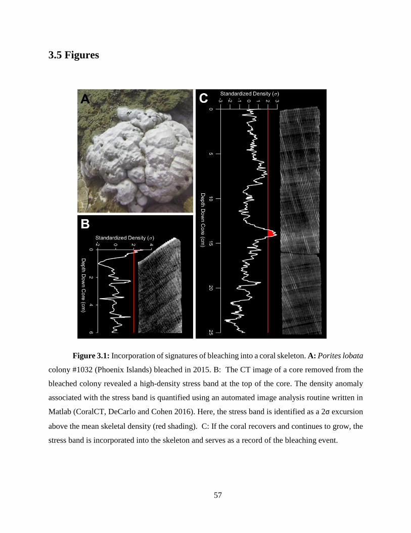
57
3.5 Figures
Figure 3.1: Incorporation of signatures of bleaching into a coral skeleton. A: Porites lobata
colony #1032 (Phoenix Islands) bleached in 2015. B: The CT image of a core removed from the
bleached colony revealed a high-density stress band at the top of the core. The density anomaly
associated with the stress band is quantified using an automated image analysis routine written in
Matlab (CoralCT, DeCarlo and Cohen 2016). Here, the stress band is identified as a 2σ excursion
above the mean skeletal density (red shading). C: If the coral recovers and continues to grow, the
stress band is incorporated into the skeleton and serves as a record of the bleaching event.
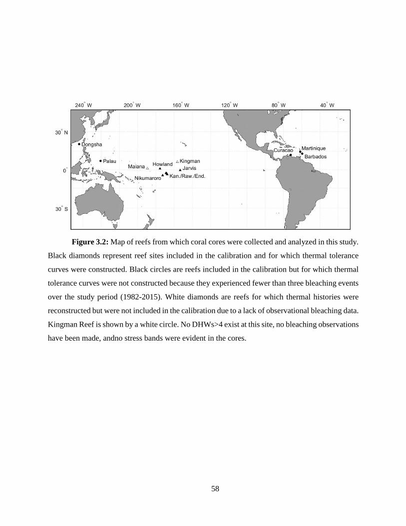
58
Figure 3.2: Map of reefs from which coral cores were collected and analyzed in this study.
Black diamonds represent reef sites included in the calibration and for which thermal tolerance
curves were constructed. Black circles are reefs included in the calibration but for which thermal
tolerance curves were not constructed because they experienced fewer than three bleaching events
over the study period (1982-2015). White diamonds are reefs for which thermal histories were
reconstructed but were not included in the calibration due to a lack of observational bleaching data.
Kingman Reef is shown by a white circle. No DHWs>4 exist at this site, no bleaching observations
have been made, andno stress bands were evident in the cores.
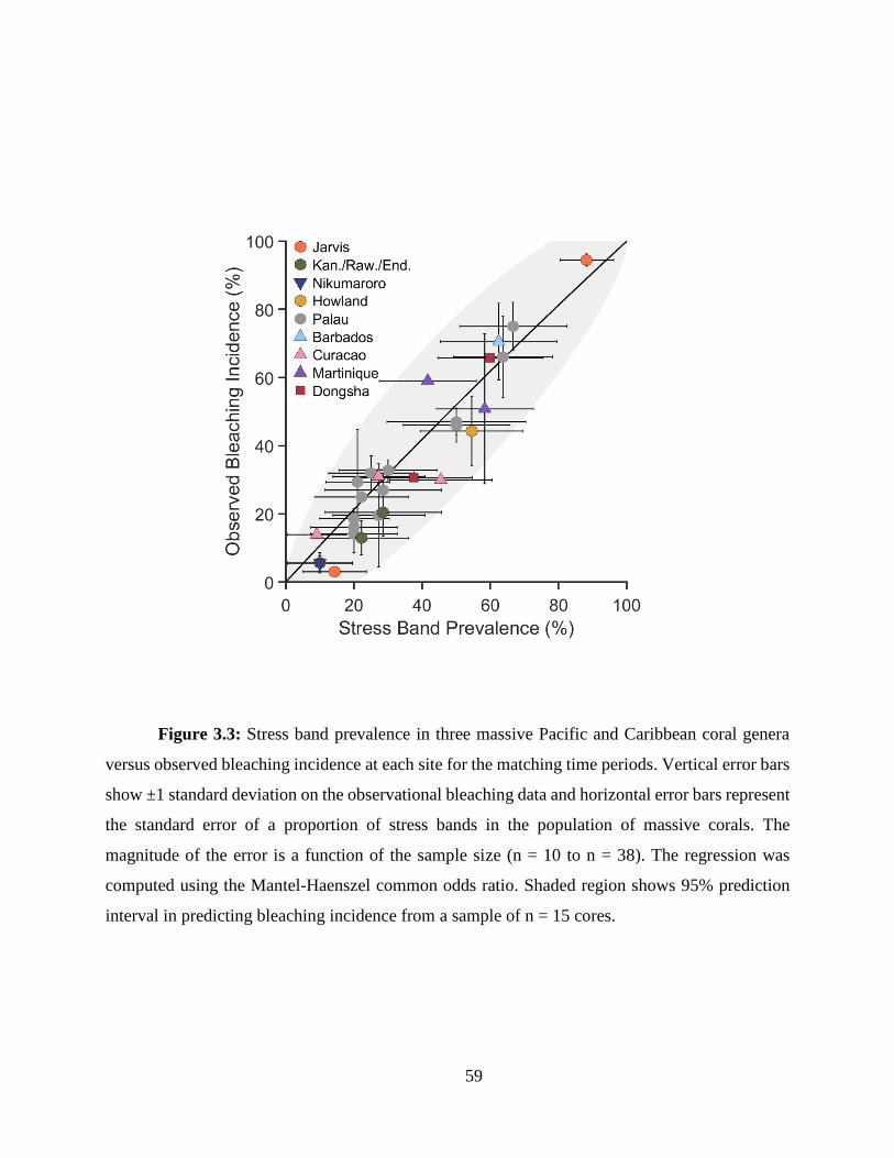
59
Figure 3.3: Stress band prevalence in three massive Pacific and Caribbean coral genera
versus observed bleaching incidence at each site for the matching time periods. Vertical error bars
show ±1 standard deviation on the observational bleaching data and horizontal error bars represent
the standard error of a proportion of stress bands in the population of massive corals. The
magnitude of the error is a function of the sample size (n = 10 to n = 38). The regression was
computed using the Mantel-Haenszel common odds ratio. Shaded region shows 95% prediction
interval in predicting bleaching incidence from a sample of n = 15 cores.
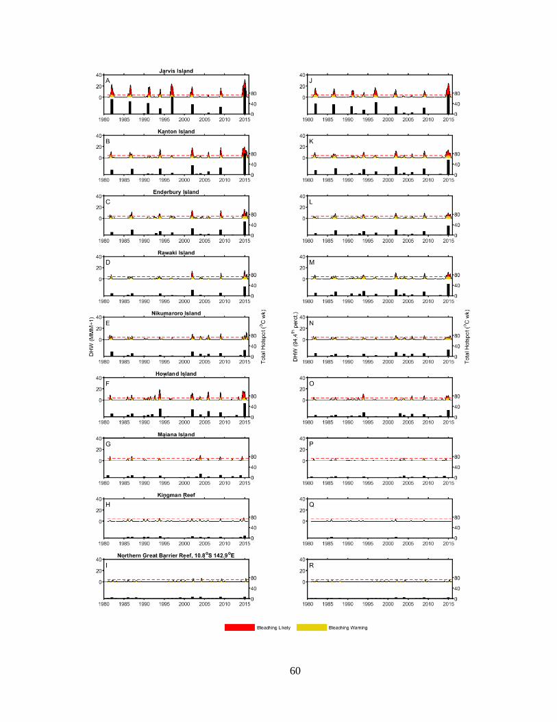
60
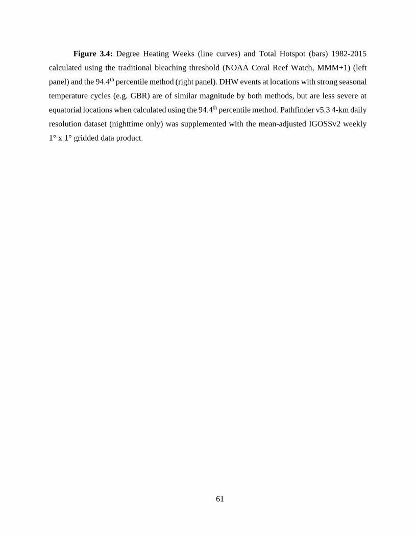
61
Figure 3.4: Degree Heating Weeks (line curves) and Total Hotspot (bars) 1982-2015
calculated using the traditional bleaching threshold (NOAA Coral Reef Watch, MMM+1) (left
panel) and the 94.4th percentile method (right panel). DHW events at locations with strong seasonal
temperature cycles (e.g. GBR) are of similar magnitude by both methods, but are less severe at
equatorial locations when calculated using the 94.4th percentile method. Pathfinder v5.3 4-km daily
resolution dataset (nighttime only) was supplemented with the mean-adjusted IGOSSv2 weekly
1° x 1° gridded data product.
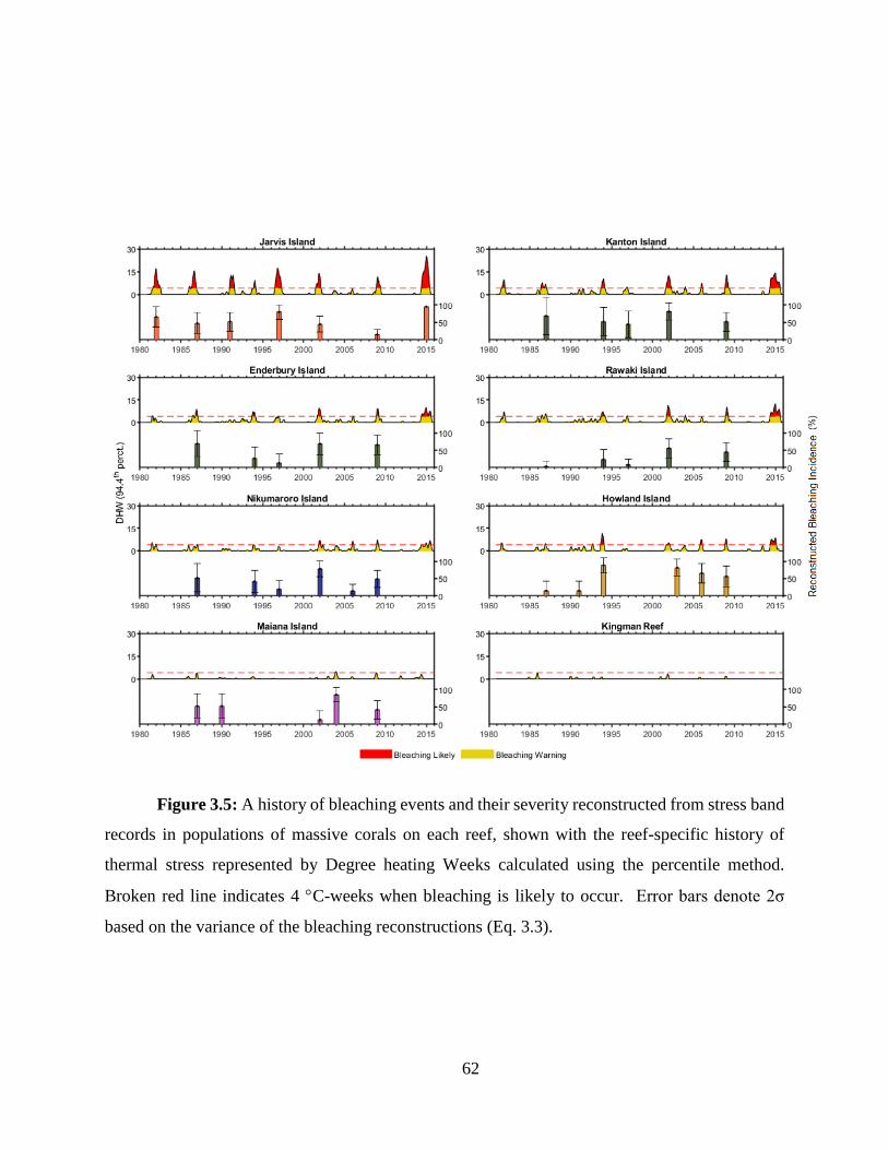
62
Figure 3.5: A history of bleaching events and their severity reconstructed from stress band
records in populations of massive corals on each reef, shown with the reef-specific history of
thermal stress represented by Degree heating Weeks calculated using the percentile method.
Broken red line indicates 4 C-weeks when bleaching is likely to occur. Error bars denote 2σ
based on the variance of the bleaching reconstructions (Eq. 3.3).
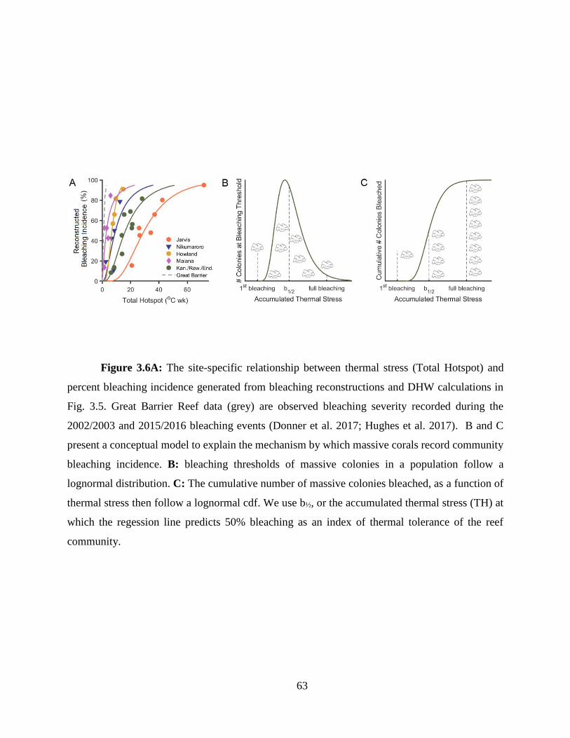
63
Figure 3.6A: The site-specific relationship between thermal stress (Total Hotspot) and
percent bleaching incidence generated from bleaching reconstructions and DHW calculations in
Fig. 3.5. Great Barrier Reef data (grey) are observed bleaching severity recorded during the
2002/2003 and 2015/2016 bleaching events (Donner et al. 2017; Hughes et al. 2017). B and C
present a conceptual model to explain the mechanism by which massive corals record community
bleaching incidence. B: bleaching thresholds of massive colonies in a population follow a
lognormal distribution. C: The cumulative number of massive colonies bleached, as a function of
thermal stress then follow a lognormal cdf. We use b½, or the accumulated thermal stress (TH) at
which the regession line predicts 50% bleaching as an index of thermal tolerance of the reef
community.
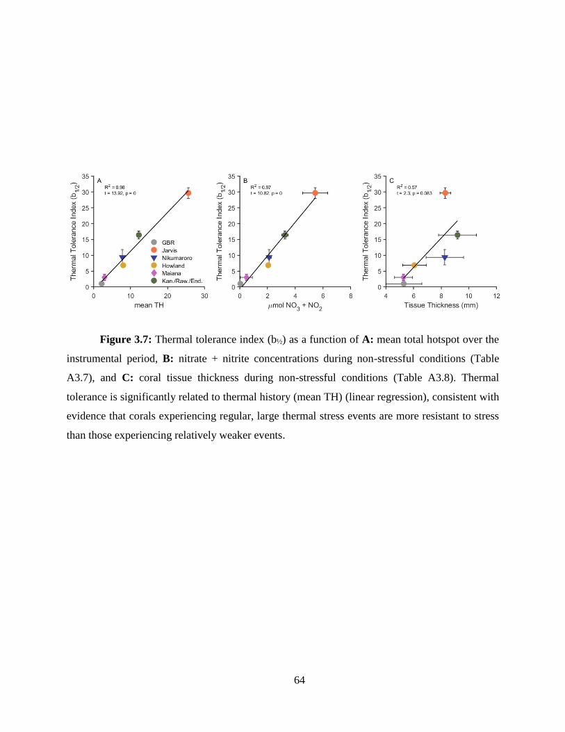
64
Figure 3.7: Thermal tolerance index (b½) as a function of A: mean total hotspot over the
instrumental period, B: nitrate + nitrite concentrations during non-stressful conditions (Table
A3.7), and C: coral tissue thickness during non-stressful conditions (Table A3.8). Thermal
tolerance is significantly related to thermal history (mean TH) (linear regression), consistent with
evidence that corals experiencing regular, large thermal stress events are more resistant to stress
than those experiencing relatively weaker events.
65
3.6 References
Alpert AE, Cohen AL, Oppo DW, Decarlo TM, Gove JM, Young CW (2016) Comparison of
equatorial Pacific sea surface temperature variability and trends with Sr/Ca records from
multiple corals. Paleoceanography 31:252–265
Ashok K, Behera SK, Rao SA, Weng H (2007) El Nino Modoki and its possible teleconnection. J
Geophys Res 112:1–27
Barkley HC, Cohen AL (2016) Skeletal records of community-level bleaching in Porites corals
from Palau. Coral Reefs 35:1407–1417
Barkley HC, Cohen AL, Brainard RE, Mollica NR, Rivera HE, Drenkard EJ, Young CW, Vargas-
Ángel B, Lohmann GP, Decarlo TM, Alpert AE, Lino KC, Oliver TA, Pietro KR, Luu VH
(2018) Repeat bleaching of a central Pacific coral reef over the past six decades (1960-2016).
Nat Biol Commun
Barkley HC, Cohen AL, Golbuu Y, Starczak VR, Decarlo TM, Shamberger KEF (2015) Changes
in coral reef communities across a natural gradient in seawater pH. Sci Adv 1–7
Barnes DJ, Lough JM (1992) Systematic variations in the depth of skeleton occupied by coral
tissue in massive colonies of Porites from the Great Barrier Reef. J Exp Mar Bio Ecol
159:113–128
Beyer HL, Kennedy E V., Beger M, Chen CA, Cinner JE, Darling ES, Eakin CM, Gates RD, Heron
SF, Knowlton N, Obura DO, Palumbi SR, Possingham HP, Puotinen M, Runting RK,
Skirving WJ, Spalding M, Wilson KA, Wood S, Veron JE, Hoegh-Guldberg O (2018) Risk-
sensitive planning for conserving coral reefs under rapid climate change. Conserv Lett e12587
Cantin NE, Cohen AL, Karnauskas KB, Tarrant AM, McCorkle DC (2010) Ocean Warming Slows
Coral Growth in the Central Red Sea. 329:322–325
Cantin NE, Lough JM (2014) Surviving coral bleaching events: Porites growth anomalies on the
great barrier reef. PLoS One 9:
Carilli J, Donner SD, Hartmann AC (2012) Historical temperature variability affects coral
response to heat stress. PLoS One 7:1–9
Carilli JE, Norris RD, Black B, Walsh SM, Mcfield M (2010) Century-scale records of coral
growth rates indicate that local stressors reduce coral thermal tolerance threshold. Glob Chang
Biol 16:1247–1257
Carilli JE, Norris RD, Black BA, Walsh SM, McField M (2009) Local stressors reduce coral
resilience to bleaching. PLoS One 4:1–5
Casey KS, Brandon TB, Cornillon P, Evans R (2010) The Past, Present, and Future of the AVHRR
Pathfinder SST Program. Oceanogr from Sp Revisit 1–375
Coles SL, Brown BE (2003) Coral bleaching-capacity for acclimatization and adaptation. Adv Mar
Biol 46:183–223
Coles SL, Jokiel PL (1977) Effects of temperature on photosynthesis and respiration in hermatypic
66
corals. Mar Biol 43:209–216
D’Angelo C, Wiedenmann J (2014) Impacts of nutrient enrichment on coral reefs: New
perspectives and implications for coastal management and reef survival. Curr Opin Environ
Sustain 7:82–93
DeCarlo TM, Cohen AL (2016) coralCT: software tool to analyze computerized tomography (CT)
scans of coral skeletal cores for calcification and bioerosion rates.
DeCarlo TM, Cohen AL (2017) Dissepiments, density bands, and signatures of thermal stress in
Porites skeletons. Coral Reefs 1–13
DeCarlo TM, Cohen AL, Barkley HC, Cobban Q, Young C, Shamberger KE, Brainard RE, Golbuu
Y (2015) Coral macrobioerosion is accelerated by ocean acidification and nutrients. Geology
43:7–10
DeCarlo TM, Cohen AL, Wong GTF, Davis KA, Lohmann P, Soong K (2017) Mass coral
mortality under local amplification of 2 °C ocean warming. Sci Rep 7:44586
Donner S (2011) An evaluation of the effect of recent temperature variability on\nthe prediction
of coral. Ecol Appl 21:1718–1730
Donner SD (2009) Coping with commitment: Projected thermal stress on coral reefs under
different future scenarios. PLoS One 4:
Donner SD, Rickbeil GJM, Heron SF (2017) A new, high-resolution global mass coral bleaching
database. PLoS One 12:1–17
Eakin CM, Morgan JA, Heron SF, Smith TB, Liu G, Alvarez-Filip L, Baca B, Bartels E, Bastidas
C, Bouchon C, Brandt M, Bruckner AW, Bunkley-Williams L, Cameron A, Causey BD,
Chiappone M, Christensen TRL, Crabbe MJC, Day O, de la Guardia E, Díaz-Pulido G,
DiResta D, Gil-Agudelo DL, Gilliam DS, Ginsburg RN, Gore S, Guzmán HM, Hendee JC,
Hernández-Delgado EA, Husain E, Jeffrey CFG, Jones RJ, Jordán-Dahlgren E, Kaufman LS,
Kline DI, Kramer PA, Lang JC, Lirman D, Mallela J, Manfrino C, Maréchal JP, Marks K,
Mihaly J, Miller WJ, Mueller EM, Muller EM, Toro CAO, Oxenford HA, Ponce-Taylor D,
Quinn N, Ritchie KB, Rodríguez S, Ramírez AR, Romano S, Samhouri JF, Sánchez JA,
Schmahl GP, Shank B V., Skirving WJ, Steiner SCC, Villamizar E, Walsh SM, Walter C,
Weil E, Williams EH, Roberson KW, Yusuf Y (2010) Caribbean corals in crisis: Record
thermal stress, bleaching, and mortality in 2005. PLoS One 5:
Emiliani C, Hudson JH, Shinn EA, George RY (1978) Oxygen and Carbon Isotopic Growth
Record in a Reef Coral from the Florida Keys and a Deep-Sea Coral from Blake Plateau.
Science (80- ) 627–628
Estep A, Sandin S, Vermeij M (2017) The State of Curaçao’s Coral Reefs.
Fine M, Gildor H, Genin A (2013) A coral reef refuge in the Red Sea. Glob Chang Biol 19:3640–
3647
Fisk DA, Done TJ (1985) Taxonomic and Bathymetric Patterns of Bleaching in Corals, Myrmidon
Reef (Queensland). Proc Fifth Int Coral Reef Congr Tahiti 6:149–154
67
Frieler K, Meinshausen M, Golly A, Mengel M, Lebek K, Donner SD, Hoegh-Guldberg O (2012)
Limiting global warming to 2 °C is unlikely to save most coral reefs. Nat Clim Chang 3:165–
170
Gleeson MW, Strong AE (1995) Applying MCSST to coral reef bleaching. Adv Sp Res 16:151–
154
Golbuu Y, Victor S, Penland L, Idip D, Emaurois C, Okaji K, Yukihira H, Iwase A, Van Woesik
R (2007) Palau’s coral reefs show differential habitat recovery following the 1998-bleaching
event. Coral Reefs 26:319–332
Grottoli G, Rodrigues LJ, Palardy JE (2006) Heterotrophic plasticity and resilience in bleached
corals. Nature 440:10–13
Hendy EJ, Lough JM, Gagan MK (2003) Historical mortality in massive Porites from the central
Great Barrier Reef, Australia: Evidence for past environmental stress? Coral Reefs 22:207–
215
Heron SF, Liu G, Eakin CM, Skirving WJ, Muller-Karger FE, Vera-Rodriguez M, de la Cour JL,
Burgess TFR, Strong AE, Geiger EF, Guild LS, Lynds S (2015) NOAA Technical Report
NESDIS 145 Climatology Development for NOAA Coral Reef Watch ’ s 5-km Product Suite.
30
Hoegh-Guldberg O, Smith GJ (1989) The effect of sudden changes in temperature, light and
salinity on the population density and export of zooxanthellae from the reef corals Stylophora
pistillata Esper and Seriatopora hystrix Dana. J Exp Mar Bio Ecol 129:279–303
Hoogenboom MO, Campbell DA, Beraud E, DeZeeuw K, Ferrier-Pagès C (2012) Effects of light,
food availability and temperature stress on the function of photosystem II and photosystem I
of coral symbionts. PLoS One 7:
van Hooidonk R, Huber M (2009) Quantifying the quality of coral bleaching predictions. Coral
Reefs 28:579–587
van Hooidonk R, Maynard J, Tamelander J, Gove J, Ahmadia G, Raymundo L, Williams G, Heron
SF, Planes S (2016) Local-scale projections of coral reef futures and implications of the Paris
Agreement. Sci Rep 6:39666
Hudson JH, Shinn EA, Halley RB, Lidz B (1976) Sclerochronology: A tool for interpreting past
environments. Geology 4:361–364
Hughes TP, Anderson KD, Connolly SR, Heron SF, Kerry JT, Lough JM, Baird AH, Baum JK,
Berumen ML, Bridge TC, Claar DC (2018) Spatial and temporal patterns of mass bleaching
of corals in the Anthropocene. Science (80- ) 359:80–83
Hughes TP, Kerry JT, Álvarez-Noriega M, Álvarez-Romero JG, Anderson KD, Baird AH,
Babcock RC, Beger M, Bellwood DR, Berkelmans R, Bridge TC, Butler IR, Byrne M, Cantin
NE, Comeau S, Connolly SR, Cumming GS, Dalton SJ, Diaz-Pulido G, Eakin CM, Figueira
WF, Gilmour JP, Harrison HB, Heron SF, Hoey AS, Hobbs J-PA, Hoogenboom MO,
Kennedy E V., Kuo C, Lough JM, Lowe RJ, Liu G, McCulloch MT, Malcolm HA,
McWilliam MJ, Pandolfi JM, Pears RJ, Pratchett MS, Schoepf V, Simpson T, Skirving WJ,
Sommer B, Torda G, Wachenfeld DR, Willis BL, Wilson SK (2017) Global warming and
68
recurrent mass bleaching of corals. Nature 543:373–377
IPCC AR5 (2014) Climate Change 2014: Synthesis Report.
Kessler WS, Kleeman R (2000) Rectification of the Madden-Julian Oscillation into the ENSO
cycle. J Clim 13:3560–3575
Liu G, Strong AE, Skirving WJ, Arzayus F (2006) Overview of NOAA Coral Reef Watch
Program’s Near-Real- Time Satellite Global Coral Bleaching Monitoring Activities. Proc
10th Int Coral Reef Symp 1783–1793
Logan CA, Dunne JP, Eakin CM, Donner SD (2014) Incorporating adaptive responses into future
projections of coral bleaching. Glob Chang Biol 20:125–139
Lough JM, Anderson KD, Hughes TP (2018) Increasing thermal stress for tropical coral reefs :
1871 – 2017. Sci Rep 1–8
Mallela J, Hetzinger S, Halfar J (2015) Thermal stress markers in Colpophyllia natans provide an
archive of site-specific bleaching events. Coral Reefs 35:181–186
Mangubhai S, Rotjan R, de Villiers S, Braun C, Carilli J, Cavin J, Cohen A, Coker D, Cook C,
Drenkard L, Gawne P, Harper S, Koethen J, Lasley R, Nand Y, Payet S, Rivera H, Sandin S,
Kiareti A, Thorrold S, Young CC, Zgliczynski B (2015) Phoenix Islands Protected Area 2015
Expedition Report.
Mantel N, Haenszel W (1959) Issue Cover Volume 22 Issue 4 April 1959 < Previous Next >
Statistical Aspects of the Analysis of Data From Retrospective Studies of Disease. J Natl
Cancer Inst 22:719–748
Matson EG (2011) Core Plugs. Encycl Mod Coral Reefs 294–296
Maynard JA, Anthony KRN, Marshall PA, Masiri I (2008) Major bleaching events can lead to
increased thermal tolerance in corals. Mar Biol 155:173–182
McClanahan TR, Ateweberhan M, Muhando C, Maina J, Mohammed SM (2007) Climate change
and spatio-temporal variation in seawater temperature effects on coral bleaching and
mortality in East Africa. Ecol Monogr 77:503–525
Obura D, Mangubhai S (2011) Coral mortality associated with thermal fluctuations in the Phoenix
Islands, 2002-2005. Coral Reefs 30:607–619
Oliver TA, Palumbi SR (2011) Do fluctuating temperature environments elevate coral thermal
tolerance? Coral Reefs 30:429–440
Pandolfi JM, Connolly SR, Marshall DJ, Cohen AL (2011) Projecting Coral Reef Futures Under
Global Warming and Ocean Acidification. Science (80- ) 333:418–422
Pratchett M, Munday P, Wilson S, Graham N, Cinner J, Bellwood D, Jones G, Polunin N,
Mcclanahan T (2008) Effects Of Climate-Induced Coral Bleaching On Coral-Reef Fishes -
Ecological And Economic Consequences.
Reynolds RW, Rayner NA, Smith TM, Stokes DC, Wang W (2002) An Improved In Situ and
Satellite SST Analysis for Climate. 15:1609–1625
69
Rodrigues LJ, Grottoli AG (2006) Calcification rate and the stable carbon, oxygen, and nitrogen
isotopes in the skeleton, host tissue, and zooxanthellae of bleached and recovering Hawaiian
corals. Geochim Cosmochim Acta 70:2781–2789
Rowan R, Knowlton N, Baker A, Jara J (1997) Landscape ecology of algal symbionts creates
variation in episodes of coral bleaching. Nature 388:265–9
Safaie A, Silbiger NJ, McClanahan TR, Pawlak G, Barshis DJ, Hench JL, Rogers JS, Williams
GJ, Davis KA (2018) High frequency temperature variability reduces the risk of coral
bleaching. Nat Commun 9:1–12
Smithers SG, Woodroffe CD (2001) Coral microatolls and 20th century sea level in the eastern
Indian Ocean. Earth Planet Sci Lett 191:173–184
Trenberth KE (1997) The Definition of El Nino. Am Meteorol Soc
Vargas-Ángel B, Looney EE, Vetter OJ, Coccagna EF (2011) Severe, widespread El Niño-
associated coral bleaching in the US Phoenix Islands. Bull Mar Sci 87:623–638
Wilkinson C (2008) Status of Coral Reefs of the World: Executive Summary. Glob Coral Reef
Monit Netw 5–28
Van Woesik R, Houk P, Isechal AL, Idechong JW, Victor S, Golbuu Y (2012) Climate-change
refugia in the sheltered bays of Palau: Analogs of future reefs. Ecol Evol 2:2474–2484
Van Woesik R, Sakai K, Ganase A, Loya Y (2011) Revisiting the winners and the losers a decade
after coral bleaching. Mar Ecol Prog Ser 434:67–76
Wooldridge SA (2009) Water quality and coral bleaching thresholds: Formalising the linkage for
the inshore reefs of the Great Barrier Reef, Australia. Mar Pollut Bull 58:745–751

70
71
Chapter 4 – Reconstructing Monthly SST
Using LA-ICPMS on Porites Corals
Nathaniel R. Mollica, Anne L. Cohen, Forrest Horton
4.1. Introduction
Seasonal oscillations are the primary mode of climate variability in the Earth’s oceans.
Sub-annual changes in sea surface temperature (SST) drive marine species migrations, supply
nutrients to the mixed layer, and constrain the habitat distributions of sessile marine organisms.
Furthermore, observations (Schubert et al. 2004; Kosaka and Xie 2013) and coupled general
circulation models (GCMs) (Seager and Vecchi 2010) indicate that seasonal temperatures in key
ocean regions drive global variability in air temperature, ocean temperature, wind velocity, and
precipitation. One key region is the central equatorial Pacific (CEP) – home to perhaps the most
important climate phenomenon in the world oceans, the El Nino Southern Oscillation (ENSO).
These coupled oscillations of SST and air pressure from east to west across the equatorial Pacific
have global impacts on climate, including droughts, monsoons, and tropical cyclones. Climate
scientists have long indexed ENSO by variations in SST in a region of the CEP known as the Nino
3.4 (5N–5S, 120W–170W). Problematically, however, SST observations are spatially
inconsistent prior to the satellite era and increasingly sparse back through time. A more complete
record of SST in the CEP and elsewhere is critical for understanding historical climate dynamics
and predicting future changes to the global climate system. In this paper, we use data obtained
from CEP corals to demonstrate that monthly SST reconstructions can be recovered using the Sr-
U paleo proxy.
4.1.1 Inconsistencies among model and observational data products in the CEP
Data coverage in the Niño 3.4 prior to the satellite era is notoriously sparse (Fig. 4.1B–D).
For example, almost no measurements were made in December 1890 (Fig. 4.1B) and large regions
72
remained unsampled into December 1970 (Fig. 4.1C). Consequently, the average error on
uninterpolated SST estimates in the Niño 3.4 prior to 1982 is ± 2 C (Fig. 4.1E). This is well within
the magnitude of the expected SST warming response to anthropogenic forcing and all but the
strongest ENSO events of the last century. Changes in observational techniques such as bucket
versus engine intake temperatures and differences in the statistical methodologies used to
interpolate the SST field from sparse inputs (Kaplan et al. 1998; Deser et al. 2010) exacerbate
uncertainties in 20th century SST records in this critical region. Such data products that augment
and interpolate these sparse measurements via statistical methods have made significant progress
towards mitigating both measurement error and spatial gaps, but are ultimately limited by data
quality and spatial resolution.
Existing SST records are insufficient for validating climate model simulations of 20th
century Pacific SST. For example, in a recent analysis of 41 CMIP5 climate models (83
simulations), SST across the central-eastern equatorial Pacific increased over the 20th century
(1900–2013 AD) in response to anthropogenic forcing. In 63% of the simulations, the east-west
SST gradient weakened over this time period due to a weakening Walker circulation. However,
these results are contrary to the mean trends in 5 observational datasets, which suggests the central
and eastern Pacific cooled over this time period, while the western Pacific warmed, strengthening
the east-west SST gradient (Coats and Karnauskas 2017; Seager et al. 2019). Such discrepancies
between models and observational data either suggest that (a) current climate models are not
capturing the response of the tropical Pacific to anthropogenic forcing or (b) that the observational
record in the early 20th century is too sparse to accurately capture SST on the relevant spatial and
temporal scales. Our inability to distinguish between these two scenarios has serious implications
for our ability to accurately project future climate. Massive corals growing on coral reefs scattered
across the equatorial Pacific have the potential to fill gaps in the observational record and thereby
shed light on this conundrum with continuous, monthly-resolved records of proxy SST spanning
the anthropogenic era.
4.1.2 Coral proxy records
Corals embed information about their oceanic environment in their skeletons as they grow,
and their annual density bands and lunar dissepiments provide internal chronometers that enable
73
reconstructions with monthly resolution. Despite the availability of coral material within the Niño
3.4 region, however, few coral-based proxy records exist and just four extend further back in time
than the mid-1900’s (Fig. 4.2A). Two of these longer records are based on coral δ18O ratios (Fig.
4.2A, B purple squares) (Evans et al. 1999; Cobb et al. 2003), which reflect a combination of
seawater temperature and seawater δ18O and thus have not been interpreted solely in terms of SST.
Two of the records are based on skeletal Sr/Ca ratios (Fig. 4.2A,B, green circles) (Nurhati
et al. 2009, 2011; Thompson et al. 2015), which can be influenced by vital effects associated with
the coral biomineralization process (de Villiers et al. 1994; Allison et al. 2001; Cohen et al. 2002;
Gaetani and Cohen 2006). Although coral Sr/Ca often varies seasonally with SST and some Sr/Ca
records capture SST variability and trends, results from this proxy have been inconsistent, lowering
confidence in the interpretation of Sr/Ca-based SST records during the pre-satellite era.
Challenges associated with interpreting coral Sr/Ca records from the Niño 3.4 region are
highlighted in Figures 4.3 and 4.4. In Figure 4.3, two long Sr/Ca records are compared with each
other and with observational SSTs over the corresponding time period. One Sr/Ca record originates
from Jarvis Island located in the bullseye of El Niño’s impact on SST (0.37°S, 160.00°W) (Fig.
4.3B, blue) (Thompson et al. 2015). The other Sr/Ca record is from Palmyra Atoll (5.87°N,
162.08°W) (Fig. 4.3B, red) (Nurhati et al. 2011). Both Sr/Ca and SST records are detrended and
presented as anomalies relative to the climatological mean.
Although confidence in the observational data from this region prior to 1982 is low (Fig.
4.1), co-variability of Jarvis and Palmyra SSTs is expected based on their respective locations and
is observed throughout the satellite era when confidence in the SST estimates is high (Fig. 4.3A,
solid lines). The Sr/Ca records, however, exhibit little co-variation (Fig. 4.3B) and are inconsistent
with each other and with the satellite SSTs. This lack of coherence indicates that factors other than
SST influence coral Sr/Ca variability.
Coral Sr/Ca records have also been used to evaluate whether eastern equatorial Pacific
(EEP) SSTs are increasing (as GCM’s and NOAA ERSST data products imply) or decreasing (as
the HADISST data product implies) in response to anthropogenic forcing (Fig. 4.4). Interpreting
Sr/Ca data generated from corals sampled at Wolf Island, Galapagos, Jimenez et al. (2018) suggest
that EEP SSTs have increased since the start of their record in 1940, implying a warming trend
74
consistent with GCM simulations over the corresponding time period. Inconsistencies among coral
Sr/Ca and between coral and satellite-based SST measurements cast doubt on this conclusion. In
Figure 4.4, Sr/Ca data from the two Wolf Island corals (blue, red lines) are shown with satellite-
era observational SSTs (black line) (1982–2010). Two results are notable. First, there is no long-
term trend in the observational data since 1982 (black dashed line) and one of Sr/Ca records (red
line), whereas the other Sr/Ca record indicates a statistically significant warming trend (blue line).
Second, the two corals have Sr/Ca means that differ by ~0.07 mmol/mol, the equivalent of 1.1 C.
Together, these inconsistencies suggest that factors other than SST influence coral Sr/Ca ratios
and that Sr/Ca proxy records are unreliable indicators of absolute temperature. Until these
inconsistencies among and between the observational and coral SST datasets are reconciled,
questions regarding the impact of anthropogenic forcing on CEP SST variability and trends will
remain unresolved.
Previous work has shown that these inconsistencies can be resolved by incorporating
additional geochemical information (i.e., the skeletal U/Ca ratio) in an improvement to the Sr/Ca
proxy called Sr-U (Decarlo et al. 2016; Alpert et al. 2017; Rodriguez et al. 2019). Here, we
demonstrate that Sr-U can be used to reconstruct monthly SSTs when paired with laser ablation
inductively coupled plasma mass spectrometry (LA-ICPMS). We present two monthly resolved
Sr-U records from the CEP that (1) capture the magnitude and phase of variability at their
respective sites through two El Niño events and (2) provide a pan-Porites and possibly pan-species
SST calibration for Sr-U. We also asses the methods capabilities in generating accurate
temperatures from old and/or subfossil skeleton that may contain diagenetic material by selectively
targeting pristine skeletal elements.
4.2 Methods
4.2.1 Coral Sr-U thermometry
Abiogenic aragonite precipitation experiments and the analysis of corals grown in culture
under controlled temperature conditions showed that coral Sr/Ca ratios are influenced by both the
mass fraction of aragonite precipitated in the calcifying fluid during biomineralization (Rayleigh
75
fractionation) and the temperature of the seawater in which skeletal growth occurs (Cohen et al.
2006, 2009; Gaetani and Cohen 2006; Gagnon et al. 2007). Based on this knowledge, and emerging
observations of systematic covariation amongst trace element ratios in coral skeletons (e.g. Sinclair
and Risk 2006) we previously developed a new coral-based paleo-thermometer, Sr-U, that uses
U/Ca to deconvolve the influence of Rayleigh fractionation from that of seawater temperature on
coral Sr/Ca (Decarlo et al. 2016; Alpert et al. 2017). U/Ca is used because it covaries with the
carbonate ion concentration of the calcifying fluid (DeCarlo et al. 2015) and is thus a proxy for the
mass fraction of aragonite precipitated by the coral.
Previous Sr-U studies (Alpert et al. 2017; Rodriguez et al. 2019) utilize multiple paired
Sr/Ca and U/Ca values generated over two to three years of coral growth to calculate a single Sr-
U value. By overlapping consecutive years, Sr-U values were generated at nominally annual
resolution. These studies found that Sr-U values generated from multiple coral species in the
Pacific and Atlantic oceans are strongly inversely correlated with observational SST over the
temperature range 22 C to 32 C. Reconstructions from these studies showed that Sr-U accurately
captures mean SSTs, multi-year variability, and century-long trends in the western tropical
Atlantic. Conversely, records based on Sr/Ca alone did not capture mean SSTs and implied a
cooling trend in the over the 20th century (Alpert et al. 2017).
Bulk sampling of coral skeletons for Sr-U thermometry, as well as Sr/Ca and δ18O analyses,
utilizes a hand-held or automated micro-drill to remove coral powder along a continuous track
parallel to the axis of maximum coral growth, attaining roughly monthly sampling resolution in
Porites corals (Fig. 4.6A,B). Sr-U thermometry uses multiple paired Sr/Ca and U/Ca ratios to
establish a Sr/Ca U/Ca regression, from which a single Sr-U value is calculated (Fig. 4.5G).
Because this regression requires tens of individual measurements, data collected over multiple
annual cycles must be used when bulk sampling thus limiting the Sr-U thermometer to
approximately one-year resolution. Building on earlier work (Fallon et al. 1999; Hathorne et al.
2011; Serrato Marks et al. 2017; Vielzeuf et al. 2018 and others), we developed a laser ablation
ICPMS technique to measure multiple Sr/Ca and U/Ca pairs within a single month of skeletal
growth and, thus, calculate monthly Sr-U values. Our method is illustrated in Figure 4.5 (D-G) and
described as follows.
76
4.2.2 Sample preparation.
Coral skeletal cores 3.5 cm-diameter (Fig. 4.6A) are slabbed along the axis of maximum
growth, scored, and broken (to avoid losing material) into 7-cm long slices, embedded in epoxy
and polished (Fig. 4.5C, D). We use a Zeiss Axioscope MosaiX microscope to image the sections
at 10 X magnification and construct a monthly chronology based on successive dissepiments (Fig.
4.5E) (DeCarlo and Cohen 2017). Microscope visualization of the section also enables us to
identify and avoid areas of skeleton that are diagenetically altered by dissolution or secondary
aragonite infilling (e.g. Cohen and Hart 2004).
4.2.3 Pressed powder standards
Our primary coral standard is a packed powder of JCP-1 (AIST Japan, and our internal
secondary coral standard is packed powder generated by subjecting a large (~500 g) piece of a
modern coral (Jardin A, Siderastrea siderea, collected in Puerto Morelos, Mexico, abbreviated
here as JAR) to a shatterbox, are analyzed between every 10 unknowns and NIST glass is analyzed
at the beginning and end of each 5-hour analytical session to ensure long-term consistency.
4.2.4 Laser ablation ICPMS
We mount the coral thick sections and our standards into a S155 vacuum chamber attached
to an ASI RESOlution-SE 193 nm ArF excimer laser ablation system. During ablation, the primary
carrier gas consists of ~1000 mL/min of argon from the mass spectrometer. We supplement this
with 500 mL/min of high purity helium and ~5 mL/min high purity dinitrogen to improve signal
strength and stability. Approximately 25 circular, 50 μm-diameter ablation spots are selected
between consecutive dissepiments, following three adjacent thecal walls in growth direction (Fig.
4.6F). This spot size is small enough to avoid centers of calcification, skeletal pores and diagenetic
areas, while providing adequate material for precise analyses (Fig. A4.1). We utilize a notably low
laser fluence (1.1 mJ/cm2, which is monitored and maintained constant in the ASI RESOlution-
SE) that produces consistent ablation and prevents rapid incision, which exacerbates down-hole
fractionation and increases the risk of drilling through the sample into epoxy. We employed a
single 64μm-diameter cleaning shot followed by a settling time of 20 s and a 50 s ablation interval
with the laser pulse rate set to 10 Hz. The homogeneity of element ratios during coral ablation
77
suggest that these settings are sufficient in mitigating any potential down-hole fractionation effects
(Fig. A4.1).
We transfer the sample gas through a signal smoothing squid on its way to an iCap Qc
mass spectrometer, on which we sequentially measure 238U, 88Sr, and 48Ca, with dwell times on
each mass of 0.5, 0.01, and 0.001 milliseconds, respectively. To determine raw elemental ratios,
we correct the counts per second measured at each mass based on the assumed normal abundances
of these isotopes in nature. We developed a laser data reduction routine, described in Appendix A.
This platform will enable users to import and process any raw data time series generated via LA-
ICPMS. The routine also includes the capability to (a) align laser spot locations with coral thin
section maps, (b) bin data into user defined intervals, (c) perform outlier analyses and screen laser
data quality, (d) conduct Sr-U regressions. It is designed to be used for a wide range of laser setups,
sampling resolutions, and compatible with multiple proxy calibrations.
In addition to the 238U, 88Sr, and 48Ca data utilized in this chapter and chapter 5 of this
thesis, we also collected 11B, 25Mg, and 138Ba measurements during each spot. While these
elements are neither examined in this chapter nor in chapter 5, each represents a valuable paleo
archive, and will be the subject of future work. It should be noted that the data reduction routine
described in Appendix A4 was constructed to process these elements as well, along with any other
future analytes with minimal modification.
4.2.5 Calculating Sr-U
We bin ~25 Sr/Ca and U/Ca pairs every 2 mm down core, with a 1 mm overlap, consistent
on average with monthly dissepiment spacings (Fig. 4.5G). We also calculate the average monthly
Sr/Ca ratio from these data (See Appendix 4A). Over both cores analyzed, 86% of monthly Sr/Ca-
U/Ca regressions were significant at the p<0.05 level (t-stat, OLS). We also tested bimonthly
binning with a 1-month overlap. This increased the number of significant regressions to 97%, and
significantly dampened variability that we attribute to outlying ablation points. This approach
yielded an average relative uncertainty for Sr-U of 0.85%.
78
4.3 Results
Using the above method, we analyzed the top ~16 cm (representing the last 10 years of
growth) from two coral cores from the CEP. Core J1222 was collected from a live coral on Jarvis
Island (0.37°S, −159.98°W) in 2017 and core N1344 was collected from a live coral on
Nikumaroro Island (4.68°S, 174.52°W) in 2018 (see locations in Figs. 4.2A and 4.11). Both corals
survived the most recent El Niño in 2015–16.
We observed a large range in both Sr/Ca and U/Ca ratios within skeleton accreted over the
course of a single month in both corals. Such fine-scale heterogeneity has been reported previously
(Allison et al. 2001; Meibom et al. 2006; Allison and Finch 2009). In our data, we find a
consistently strong, positive correlation (average r2 = 0.82) between each of the ~25 Sr/Ca and
U/Ca ratios collected between successive dissepiments (i.e., within a single month of growth). The
wide range in Sr/Ca and U/Ca ratios over small length scales and their strong covariation indicates
that coral Sr/Ca is strongly influenced by the mass fraction of aragonite (indicated by U/Ca)
precipitated by the coral from each batch of calcifying fluid (Gaetani et al. 2011; DeCarlo et al.
2015).
4.3.1 Regression of laser Sr-U and Sr/Ca on SST
In Figure 4.6A, the Sr-U SST relationships for J1222 (blue) and N1344 (red) are plotted
together. Monthly resolved Sr-U values from both corals show a strong, inverse correlation with
monthly resolved SST over the temperature range 24–30.5 C, as predicted by Sr-U theory
(DeCarlo et al., 2016). Further, the Sr-U SST relationships in the two corals are indistinguishable
from each other (Fig. 4.10C). This result indicates the potential for a universal Sr-U SST
calibration for Porites similar to that observed in bulk analyses of Atlantic coral species
(Rodriguez et al., 2019). The calibration we derive from these results is as follows:
𝑺𝑺𝑻 (°𝑪) = −13.244 ± 0.594 × 𝑺𝒓𝑼 + 146.88 ± 5.33
Figure 4.6B shows the corresponding monthly Sr/Ca SST relationships. Sr/Ca from both
corals also show an inverse correlation with SST, but the residuals from the two corals form two
distinct populations (Fig. 4.6D), indicating that the Sr/Ca SST relationship differs between the two
79
corals, as has been shown for analogous bulk measurements. These coral-specific relationships
confirm that factors other than temperature influence coral Sr/Ca, even at this sampling scale.
4.3.2 Jarvis Island record
In Figure 4.7, we present a continuous, 10-year, monthly-resolved Sr-U time-series
generated from J1222 and N1344 using laser ablation, as well as the monthly Sr/Ca record
generated by averaging all Sr/Ca values in each bin. The proxy datasets are plotted against satellite
(OISST) data (black lines). Both Sr-U and Sr/Ca time-series are scaled to the SST data by
calibrating the first two years of each time-series against SST and applying the calibration to the
reminder of each record. It is notable that both Sr-U and Sr/Ca produce variability with consistent
phase as the El Niño SST anomalies in 2010 and 2015. However, the relationship between Sr-U
and SST remains consistent through the record, whereas the Sr/Ca SST relationship does not. The
Sr/Ca record implies a significantly cooler 2010 ST anomaly than indicated by the instrumental
dataset, as well as a warming trend over this period that is not apparent in the satellite record.
4.3.2 Nikumaroro Island record
We constructed a second, continuous 10-year, monthly-resolved Sr-U time-series from
coral N1344, a Porites coral cored on Nikumaroro Island (4.68°S, 174.52°W) in 2018 (Fig. 4.9 B).
Nikumaroro is located outside the Niño 3.4 and further into the Niño 4.0 region, south of the
equator. We applied the same Sr-U SST calibration as above (i.e., based on the top 2 years of the
Jarvis coral) to the Sr-U data generated from the Nikumaroro coral. We find that Sr-U captures the
mean SST at Nikumaroro, as well as the timing and amplitude of SST variability in the
observational record, including the existence and relative amplitudes of the 2009–10 and 2015–16
El Niños. Conversely, the Sr/Ca-only record derived from the same data returns SSTs that are too
warm (Fig. 4.7D).
4.4 Discussion
As in calibrations derived from bulk sampling (Decarlo et al. 2016; Alpert et al. 2017;
Rodriguez et al. 2019), LA-ICPMS Sr-U shows promise in mitigating vital effects that produce
80
decoupling and coral to coral offsets common in Sr/Ca records. Both Sr-U records correlate with
SST on both a seasonal (i.e. 3 month moving average, r = 0.79, p <1e-33 for J1222; r = 0.42, p
<1e-5 for N1344; r =0.84, p <1e-72 combined) and ENSO (i.e. 1-year moving average, r = 0.83, p
<1e-40 for J1222; r = 0.33, p <1e-3 for N1344; r =0.80, p <1e-62 combined) time scale, although
N1344 has a lower Pearson coefficient which is likely due to the smaller amplitude of SST
variability resulting in a lower signal to noise ratio. Additionally, there remain slight discrepancies
between Sr-U and instrumental SST (Fig. 4.7A,C). Notably these decouplings tend to occur during
warm periods (e.g. J1222 Sr-U does not reach the peak SST recorded by satellite during the 2010
El Niño). Several factors may have resulted in these discrepancies, namely a deviation of local
SST from regional SST, fluctuations in coral growth rate not reflected in sampling, or some
component of coral vital effects not accounted for by the Sr-U proxy. While a definitive cause
cannot be identified, here we provide a discussion of the likelihood and implications of each
possibility.
An ever-present concern when generating proxy records from coral archives is the
heterogeneity of the reef environment. Due to the complex bathymetry and resultant
hydrodynamics of coral reefs, these environments are subject to systematic temperature variability
on kilometer to meter scales (e.g. Venegas et al. 2019). Such spatial variability has been studied
on Jarvis island (Barkley et al. 2018; Venegas et al. 2019), and found to vary by up to 0.5°C degrees
around the east side of the island, and up to 2°C between the east and the west (where upwelling
from the EUC occurs). The cores used in this analysis were selected opportunistically, and
although in situ logger data has been collected at several locations on Jarvis island, the closest
logger to colony J1222 was ~700 m away. At Nikumaroro island, loggers were deployed closer to
the colony (~50 m), but for only part of the duration of the record (2012-2015) (Mollica et al.
2019). Despite these uncertainties, high resolution satellite SST (Pathfinder v5.3) is consistent with
loggers deployed nearest to the sampled colonies both on Jarvis and Nikumaroro. Furthermore,
the relationship between Sr-U and satellite SST is consistent between both colonies (Fig. 4.6), a
result expected given the premise of the Sr-U thermometer (Decarlo et al. 2016) and the results of
bulk analyses (Alpert et al. 2017; Rodriguez et al. 2019). However, the observed deviations in the
Sr-U record may be a result of this imperfect control on measured SST.
81
Minor discrepancies in the agreement between the Sr-U and satellite SST may also be a
result of variability in the coral growth rate. Where possible, monthly age models were verified by
dissepiment, however during periods of the record where dissepiment preservation was poor a
homogenous (i.e. 2mm bin with 1mm overlap sampling rate). If seasonal growth rates vary
substantially during these periods, as has been seen in some higher latitude corals (DeCarlo and
Cohen 2017), a bias towards faster growing time periods may occur. Additionally, the species of
the two records, Porites, is known to not only calcify skeleton at the exterior surface of the colony,
but also to thicken existing skeletal elements throughout the tissue layer (in these cores ~7mm) in
a process called bio-smoothing (Barnes and Lough 1993; Gagan et al. 2012). However, these
effects have been found to be limited to the top ~10% of the tissue layer in Porites corals (Mollica
et al. 2018) and is lessened for faster growing colonies (Gagan et al. 2012). Given the growth rate
of our corals (J1222 = 1.79 cm yr-1, N1344 = 2.03 cm yr-1), it is unlikely that the bio-smoothing
process has had substantial impact on the overall record (especially when binned to 1mm
resolution) but may account for short discrepancies during periods of low growth rate.
It should be noted however bio-smoothing prohibits our current sampling method (i.e. 50
µm spot size, which accounts for most of an individual skeletal element) from examining SST
fluctuations at higher temporal resolution. Efforts in examining diurnal variability in element ratios
are better suited to techniques capable of higher spatial resolution, e.g. Secondary Ion Mass
Spectrometry (SIMS). While several studies have examined coral skeletal element ratios at this
scale (e.g. Hart and Cohen 1996; Allison and Finch 2007), the current method of Sr-U calculation
makes its use prohibitive at the needed resolution.
Discrepancies between ocean temperature around a colony and the Sr-U recorded in the
coral skeleton could of course also be a result of the Sr-U proxy failing to record the correct SST.
This could arise from erroneous measurements of either the Sr/Ca or U/Ca ratio of the coral
skeleton, or a failure of the method to fully counteract vital effects in coral calcification at the
monthly scale. While the precision of our consistency standard across all runs (see Appendix A)
makes significant analytical error an unlikely factor, this analysis represents the first test of the Sr-
U proxy at high resolution. When sampling 50 µm spots over a variety of skeletal elements in
multiple corallites, heterogeneity between types of skeletal element (e.g. endothecal vs. exothecal)
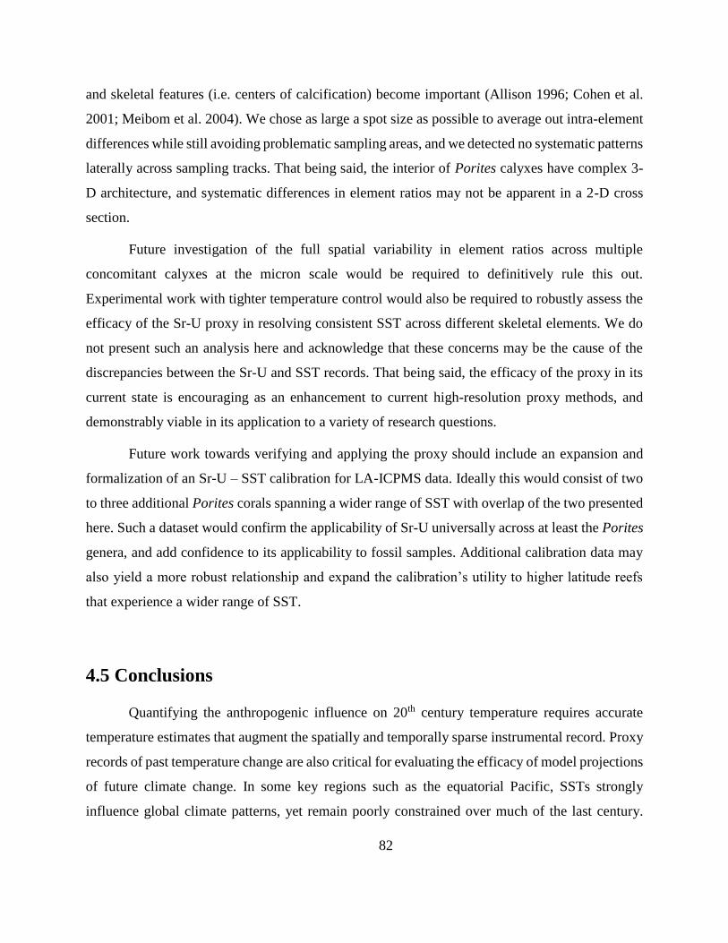
82
and skeletal features (i.e. centers of calcification) become important (Allison 1996; Cohen et al.
2001; Meibom et al. 2004). We chose as large a spot size as possible to average out intra-element
differences while still avoiding problematic sampling areas, and we detected no systematic patterns
laterally across sampling tracks. That being said, the interior of Porites calyxes have complex 3-
D architecture, and systematic differences in element ratios may not be apparent in a 2-D cross
section.
Future investigation of the full spatial variability in element ratios across multiple
concomitant calyxes at the micron scale would be required to definitively rule this out.
Experimental work with tighter temperature control would also be required to robustly assess the
efficacy of the Sr-U proxy in resolving consistent SST across different skeletal elements. We do
not present such an analysis here and acknowledge that these concerns may be the cause of the
discrepancies between the Sr-U and SST records. That being said, the efficacy of the proxy in its
current state is encouraging as an enhancement to current high-resolution proxy methods, and
demonstrably viable in its application to a variety of research questions.
Future work towards verifying and applying the proxy should include an expansion and
formalization of an Sr-U – SST calibration for LA-ICPMS data. Ideally this would consist of two
to three additional Porites corals spanning a wider range of SST with overlap of the two presented
here. Such a dataset would confirm the applicability of Sr-U universally across at least the Porites
genera, and add confidence to its applicability to fossil samples. Additional calibration data may
also yield a more robust relationship and expand the calibration’s utility to higher latitude reefs
that experience a wider range of SST.
4.5 Conclusions
Quantifying the anthropogenic influence on 20th century temperature requires accurate
temperature estimates that augment the spatially and temporally sparse instrumental record. Proxy
records of past temperature change are also critical for evaluating the efficacy of model projections
of future climate change. In some key regions such as the equatorial Pacific, SSTs strongly
influence global climate patterns, yet remain poorly constrained over much of the last century.
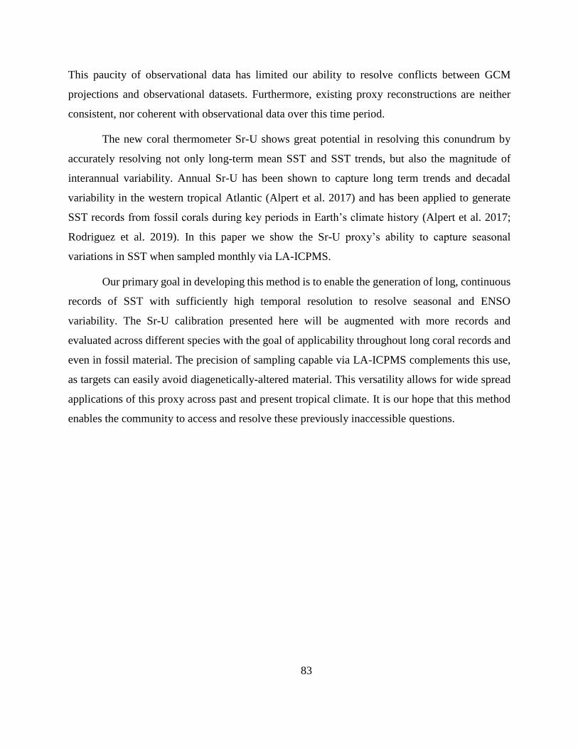
83
This paucity of observational data has limited our ability to resolve conflicts between GCM
projections and observational datasets. Furthermore, existing proxy reconstructions are neither
consistent, nor coherent with observational data over this time period.
The new coral thermometer Sr-U shows great potential in resolving this conundrum by
accurately resolving not only long-term mean SST and SST trends, but also the magnitude of
interannual variability. Annual Sr-U has been shown to capture long term trends and decadal
variability in the western tropical Atlantic (Alpert et al. 2017) and has been applied to generate
SST records from fossil corals during key periods in Earth’s climate history (Alpert et al. 2017;
Rodriguez et al. 2019). In this paper we show the Sr-U proxy’s ability to capture seasonal
variations in SST when sampled monthly via LA-ICPMS.
Our primary goal in developing this method is to enable the generation of long, continuous
records of SST with sufficiently high temporal resolution to resolve seasonal and ENSO
variability. The Sr-U calibration presented here will be augmented with more records and
evaluated across different species with the goal of applicability throughout long coral records and
even in fossil material. The precision of sampling capable via LA-ICPMS complements this use,
as targets can easily avoid diagenetically-altered material. This versatility allows for wide spread
applications of this proxy across past and present tropical climate. It is our hope that this method
enables the community to access and resolve these previously inaccessible questions.
84
4.6 Figures
Figure 4.1: Pacific SST anomaly during the peak of the 2015–2016 El Niño heatwave
(OISST v2, ¼° daily anomaly). The black rectangle outlines the Niño 3.4 region most commonly
used to define ENSO. (B-D) SST measurements across the Pacific basin in December 1890 (B),
December 1970 (C), and December 2015 (D) reveal the paucity of data in the 3.4 region (rectangle)
prior to the satellite era. (E) The number of observations in the Nino 3.4 over the course of the
instrumental record (dark green line). Data paucity prior to the satellite era leads to large
uncertainties on the uninterpolated SSTs (light grey shading represents HADSST); dark grey
shading is the 2 uncertainty post-1982 (i.e., satellite) era.
85
.
Figure 4.2: (A) Spatial correlation of Pacific basin SST (OISST v2, ¼° daily SST) with
the Niño 3.4 SST (black box). Existing coral proxy SST records are shown. Sr/Ca records are tan
circles; δ18O records are purple squares. (B) shows existing coral proxy records in the Niño 3.4
region. Symbol size represents the relative length of each record. (C) and (D) show numbers and
lengths of existing Sr/Ca (C) and δ18O (D) coral proxy records across the Pacific (light lines) and
Niño 3.4 (bold lines).
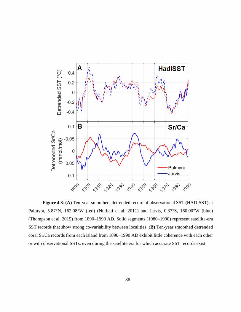
86
Figure 4.3: (A) Ten-year smoothed, detrended record of observational SST (HADISST) at
Palmyra, 5.87°N, 162.08°W (red) (Nurhati et al. 2011) and Jarvis, 0.37°S, 160.00°W (blue)
(Thompson et al. 2015) from 1890–1990 AD. Solid segments (1980–1990) represent satellite-era
SST records that show strong co-variability between localities. (B) Ten-year smoothed detrended
coral Sr/Ca records from each island from 1890–1990 AD exhibit little coherence with each other
or with observational SSTs, even during the satellite era for which accurate SST records exist.
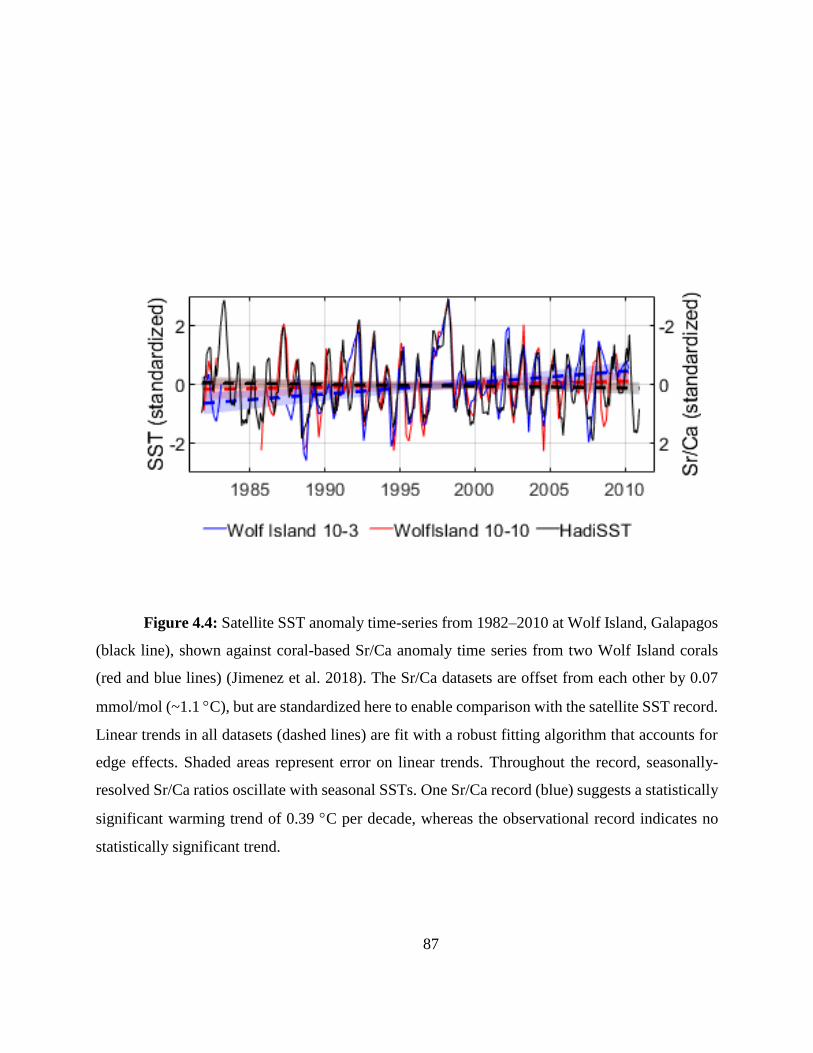
87
Figure 4.4: Satellite SST anomaly time-series from 1982–2010 at Wolf Island, Galapagos
(black line), shown against coral-based Sr/Ca anomaly time series from two Wolf Island corals
(red and blue lines) (Jimenez et al. 2018). The Sr/Ca datasets are offset from each other by 0.07
mmol/mol (~1.1 C), but are standardized here to enable comparison with the satellite SST record.
Linear trends in all datasets (dashed lines) are fit with a robust fitting algorithm that accounts for
edge effects. Shaded areas represent error on linear trends. Throughout the record, seasonally-
resolved Sr/Ca ratios oscillate with seasonal SSTs. One Sr/Ca record (blue) suggests a statistically
significant warming trend of 0.39 C per decade, whereas the observational record indicates no
statistically significant trend.
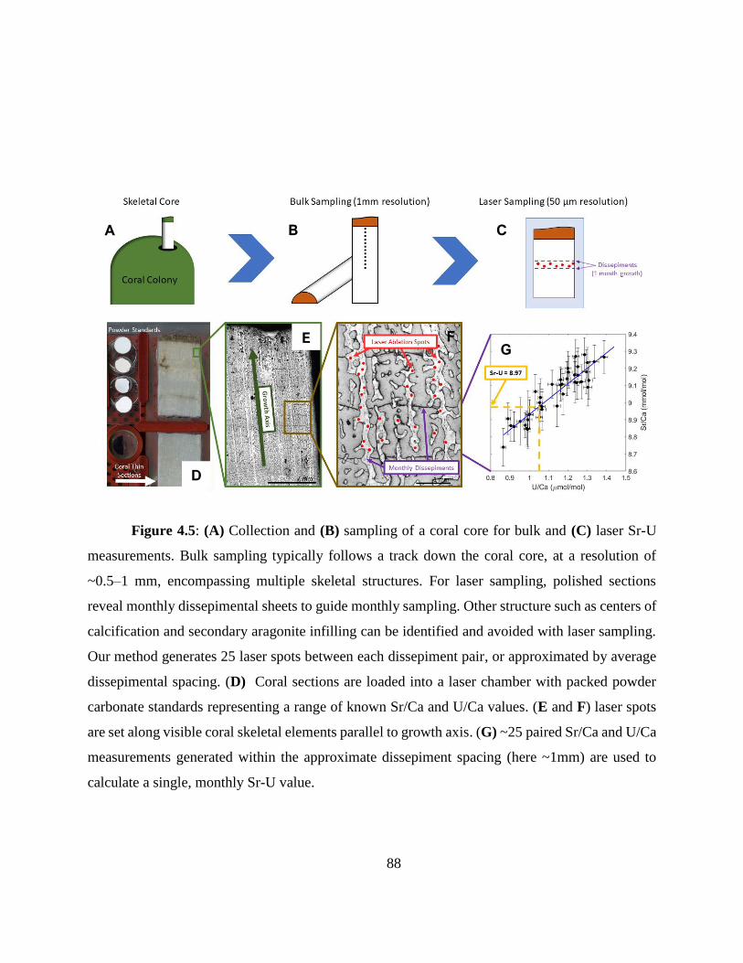
88
Figure 4.5: (A) Collection and (B) sampling of a coral core for bulk and (C) laser Sr-U
measurements. Bulk sampling typically follows a track down the coral core, at a resolution of
~0.5–1 mm, encompassing multiple skeletal structures. For laser sampling, polished sections
reveal monthly dissepimental sheets to guide monthly sampling. Other structure such as centers of
calcification and secondary aragonite infilling can be identified and avoided with laser sampling.
Our method generates 25 laser spots between each dissepiment pair, or approximated by average
dissepimental spacing. (D) Coral sections are loaded into a laser chamber with packed powder
carbonate standards representing a range of known Sr/Ca and U/Ca values. (E and F) laser spots
are set along visible coral skeletal elements parallel to growth axis. (G) ~25 paired Sr/Ca and U/Ca
measurements generated within the approximate dissepiment spacing (here ~1mm) are used to
calculate a single, monthly Sr-U value.
C B A
D
E F G
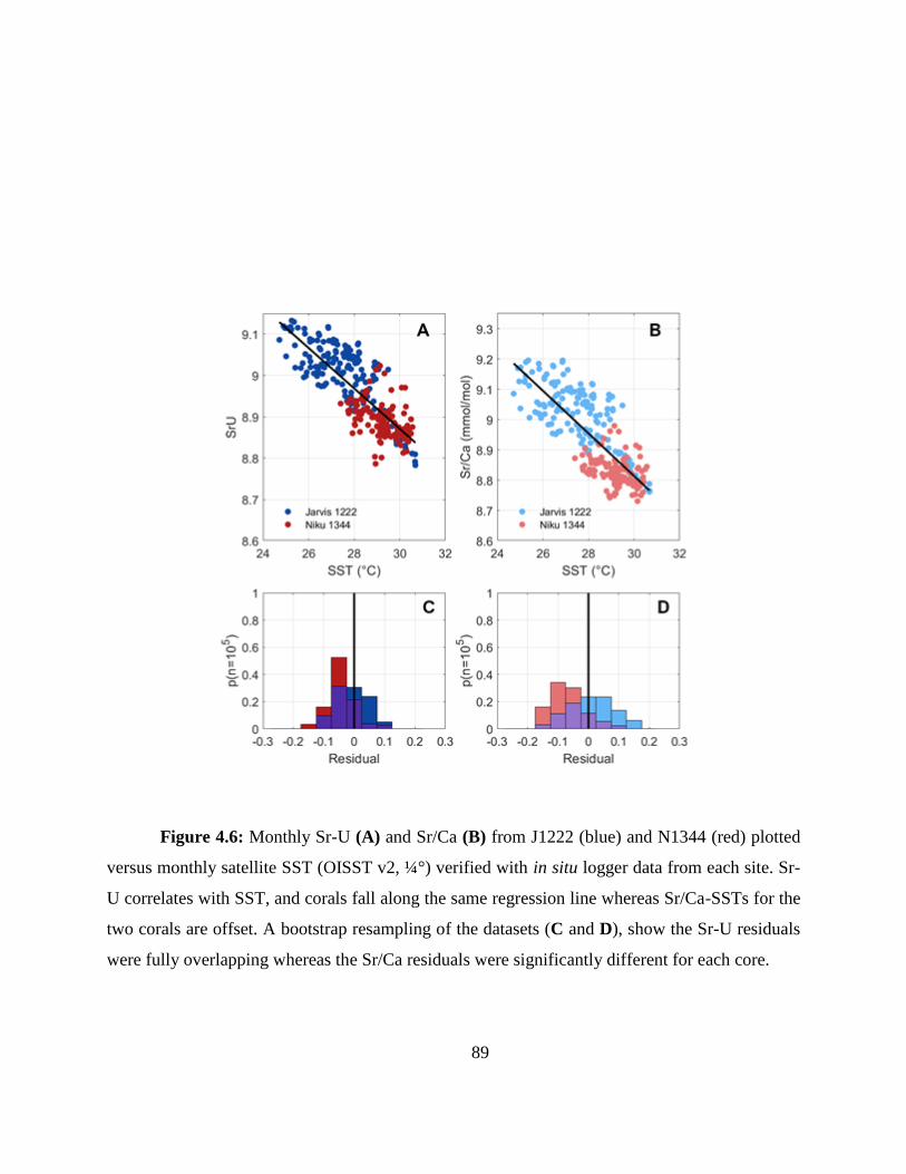
89
Figure 4.6: Monthly Sr-U (A) and Sr/Ca (B) from J1222 (blue) and N1344 (red) plotted
versus monthly satellite SST (OISST v2, ¼°) verified with in situ logger data from each site. Sr-
U correlates with SST, and corals fall along the same regression line whereas Sr/Ca-SSTs for the
two corals are offset. A bootstrap resampling of the datasets (C and D), show the Sr-U residuals
were fully overlapping whereas the Sr/Ca residuals were significantly different for each core.
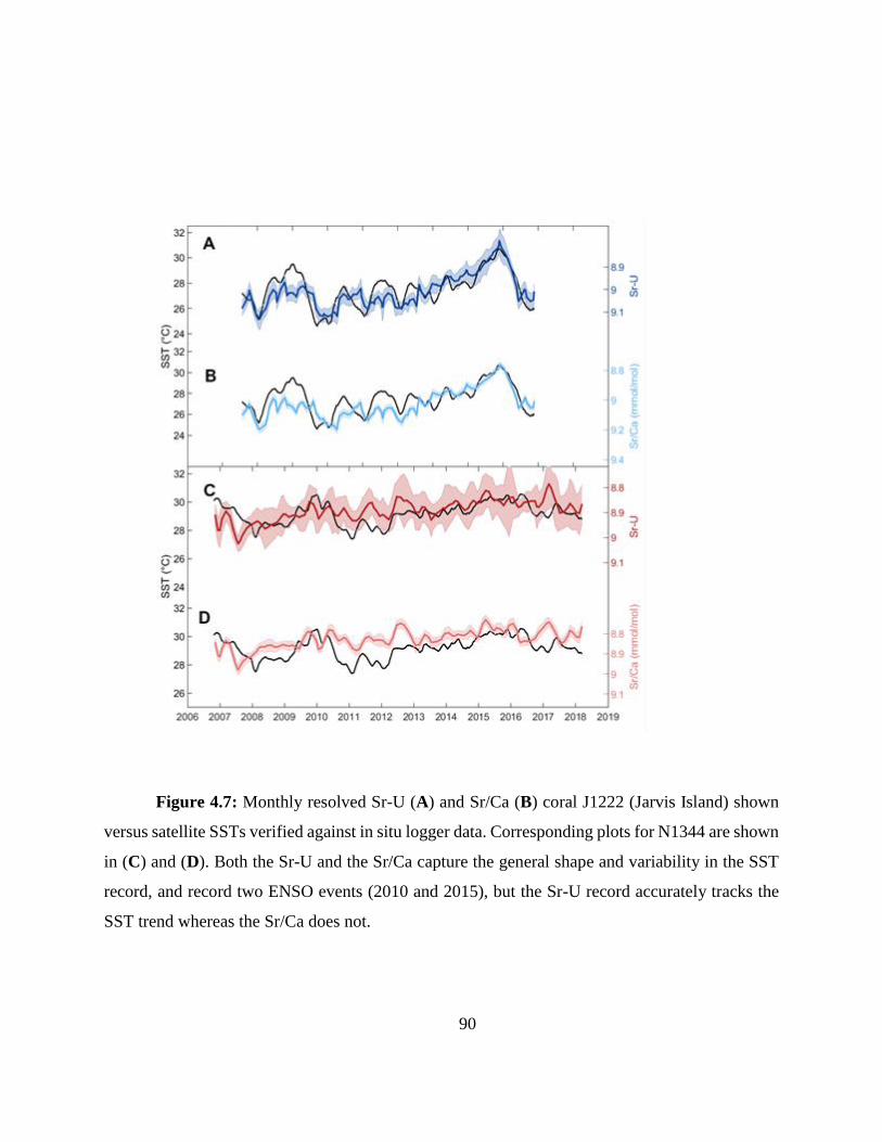
90
Figure 4.7: Monthly resolved Sr-U (A) and Sr/Ca (B) coral J1222 (Jarvis Island) shown
versus satellite SSTs verified against in situ logger data. Corresponding plots for N1344 are shown
in (C) and (D). Both the Sr-U and the Sr/Ca capture the general shape and variability in the SST
record, and record two ENSO events (2010 and 2015), but the Sr-U record accurately tracks the
SST trend whereas the Sr/Ca does not.
91
4.7 References
Allison N (1996) Geochemical anomalies in coral skeletons and their possible implications for
paleoenvironmental analyses. Mar Chem
Allison N, Finch AA (2007) High temporal resolution Mg/Ca and Ba/Ca records in modern Porites
lobata corals. Geochemistry, Geophys Geosystems 8:
Allison N, Finch AA (2009) Reproducibility of minor and trace element determinations in Porites
coral skeletons by secondary ion mass spectrometry. Geochemistry, Geophys Geosystems
10:
Allison N, Finch AA, Sutton SR, Newville M (2001) Strontium heterogeneity and speciation in
coral aragonite: Implications for the strontium paleothermometer. Geochim Cosmochim Acta
65:2669–2676
Alpert AE, Cohen AL, Oppo DW, DeCarlo TM, Gaetani GA, Hernandez-Delgado EA, Winter A,
Gonneea ME (2017) Twentieth century warming of the tropical Atlantic captured by Sr-U
paleothermometry. Paleoceanography 32:146–160
Barkley HC, Cohen AL, Brainard RE, Mollica NR, Rivera HE, Drenkard EJ, Young CW, Vargas-
Ángel B, Lohmann GP, Decarlo TM, Alpert AE, Lino KC, Oliver TA, Pietro KR, Luu VH
(2018) Repeat bleaching of a central Pacific coral reef over the past six decades (1960-2016).
Nat Biol Commun
Barnes DJ, Lough JM (1993) On the nature and causes of density banding in massive coral
skeletons. J Exp Mar Bio Ecol 167:91–108
Coats S, Karnauskas KB (2017) Are Simulated and Observed Twentieth Century Tropical Pacific
Sea Surface Temperature Trends Significant Relative to Internal Variability? Geophys Res
Lett 44:
Cobb KM, Charles CD, Cheng H, Edwards RL (2003) El Niño/Southern Oscillation and tropical
Pacific climate during the last millennium. Nature 424:271–276
Cohen AL, Gaetani GA, Lundälv T, Corliss BH, George RY (2006) Compositional variability in
a cold-water scleractinian, Lophelia pertusa: New insights into “vital effects.” Geochemistry,
92
Geophys Geosystems 7:
Cohen AL, Hart SR (2004) Deglacial sea surface temperatures of the western tropical Pacific: A
new look at old coral. Paleoceanography 19:1–6
Cohen AL, Layne GD, Hart SR, Lobel PS (2001) Kinetic control of skeletal Sr/Ca in a symbiotic
coral: Implications for the paleotemperature proxy. Paleoceanography 16:20–26
Cohen AL, McCorkle DC, De Putron S, Gaetani GA, Rose KA (2009) Morphological and
compositional changes in the skeletons of new coral recruits reared in acidified seawater:
Insights into the biomineralization response to ocean acidification. Geochemistry, Geophys
Geosystems 10:
Cohen AL, Owens KE, Layne GD, Shimizu N (2002) The effect of algal symbionts on the accuracy
of Sr/Ca paleotemperatures from coral. Science (80- ) 296:331–333
DeCarlo TM, Cohen AL (2017) Dissepiments, density bands, and signatures of thermal stress in
Porites skeletons. Coral Reefs 1–13
Decarlo TM, Gaetani GA, Cohen AL, Foster GL, Alpert AE, Stewart JA (2016) Coral Sr-U
thermometry. Paleoceanography 626–638
DeCarlo TM, Gaetani GA, Holcomb M, Cohen AL (2015) Experimental determination of factors
controlling U/Ca of aragonite precipitated from seawater: Implications for interpreting coral
skeleton. Geochim Cosmochim Acta 162:151–165
Deser C, Phillips AS, Alexander MA (2010) Twentieth century tropical sea surface temperature
trends revisited. Geophys Res Lett 37:1–6
Evans MN, Fairbanks RG, Rubenstone JL (1999) The thermal oceanographic signal of El Niño
reconstructed from a Kiritimati Island coral. J Geophys Res Ocean 104:13409–13421
Fallon SJ, McCulloch MT, Van Woesik R, Sinclair DJ (1999) Corals at their latitudinal limits:
Laser ablation trace element systematics in Porites from Shirigai Bay, Japan. Earth Planet Sci
Lett 172:221–238
Gaetani GA, Cohen AL (2006) Element partitioning during precipitation of aragonite from
seawater: A framework for understanding paleoproxies. Geochim Cosmochim Acta 70:4617–
93
4634
Gaetani GA, Cohen AL, Wang Z, Crusius J (2011) Rayleigh-based, multi-element coral
thermometry: A biomineralization approach to developing climate proxies. Geochim
Cosmochim Acta 75:1920–1932
Gagan MK, Dunbar GB, Suzuki A (2012) The effect of skeletal mass accumulation in Porites on
coral Sr/Ca and ??18O paleothermometry. Paleoceanography 27:1–16
Gagnon AC, Adkins JF, Fernandez DP, Robinson LF (2007) Sr/Ca and Mg/Ca vital effects
correlated with skeletal architecture in a scleractinian deep-sea coral and the role of Rayleigh
fractionation. Earth Planet Sci Lett 261:280–295
Hart SR, Cohen AL (1996) An ion probe study of annual cycles of Sr / Ca and other trace elements
in corals. Geochim Cosmochim Acta 60:3075–3084
Hathorne EC, Felis T, James RH, Thomas A (2011) Laser ablation ICP-MS screening of corals for
diagenetically affected areas applied to Tahiti corals from the last deglaciation. Geochim
Cosmochim Acta 75:1490–1506
Jimenez G, Cole JE, Thompson DM, Tudhope AW (2018) Northern Galápagos Corals Reveal
Twentieth Century Warming in the Eastern Tropical Pacific. Geophys Res Lett 45:1981–1988
Kaplan A, Cane MA, Clement AC, Blumenthal MB, Rajagopalan B (1998) Analyses of global sea
surface temperature 1856-1991. J Geophys Res 103:
Kosaka Y, Xie S (2013) Recent global-warming hiatus tied to equatorial Pacific surface cooling.
Nature 501:403–407
Meibom A, Cuif JP, Hillion F, Constantz BR, Juillet-Leclerc A, Dauphin Y, Watanabe T, Dunbar
RB (2004) Distribution of magnesium in coral skeleton. Geophys Res Lett 31:1–4
Meibom A, Yurimoto H, Cuif JP, Domart-Coulon I, Houlbreque F, Constantz B, Dauphin Y,
Tambutté E, Tambutté S, Allemand D, Wooden J, Dunbar R (2006) Vital effects in coral
skeletal composition display strict three-dimensional control. Geophys Res Lett 33:2–5
Mollica NR, Cohen AL, Alpert AE, Barkley HC, Brainard RE, Carilli JE, Decarlo TM, Drenkard
EJ, Lohmann P, Mangubhai S (2019) Skeletal records of bleaching reveal different thermal
94
thresholds of Pacific coral reef assemblages. Coral Reefs
Mollica NR, Guo W, Cohen AL, Huang K-F, Foster GL, Donald HK, Solow AR (2018) Ocean
Acidification Affects Coral Growth by Reducing Skeletal Density. Proc Natl Acad Sci
Nurhati IS, Cobb KM, Charles CD, Dunbar RB (2009) Late 20th century warming and freshening
in the central tropical Pacific. Geophys Res Lett 36:2–5
Nurhati IS, Cobb KM, Di Lorenzo E (2011) Decadal-scale SST and salinity variations in the
central tropical pacific: Signatures of natural and anthropogenic climate change. J Clim
24:3294–3308
Rodriguez LG, Cohen AL, Ramirez W, Oppo DW, Pourmand A, Edwards RL, Alpert AE, Mollica
N (2019) Mid-Holocene, Coral-Based Sea Surface Temperatures in the Western Tropical
Atlantic. Paleoceanogr Paleoclimatology 34:1234–1245
Schubert SD, Suarez MJ, Pegion PJ, Koster RD, Bacmeister JT (2004) Causes of Long-Term
Drought in the U . S . Great Plains. Am Meteorol Soc 485–503
Seager R, Cane M, Henderson N, Lee D, Abernathey R (2019) Strengthening tropical Pacific zonal
sea surface temperature gradient consistent with rising greenhouse gases. Nat Clim Chang 9:
Seager R, Vecchi GA (2010) Greenhouse warming and the 21st century hydroclimate of
southwestern North America. Proc Natl Acad Sci
Serrato Marks G, LaVigne M, Hill TM, Sauthoff W, Guilderson TP, Roark EB, Dunbar RB,
Horner TJ (2017) Reproducibility of Ba/Ca variations recorded by northeast Pacific bamboo
corals. Paleoceanography 32:966–979
Sinclair DJ, Risk MJ (2006) A numerical model of trace-element coprecipitation in a
physicochemical calcification system: Application to coral biomineralization and trace-
element “vital effects.” Geochim Cosmochim Acta 70:3855–3868
Thompson DM, Cole JE, Shen GT, Tudhope AW, Meehl GA (2015) Early twentieth-century
warming linked to tropical Pacific wind strength. Nat Geosci 8:117–121
Venegas RM, Oliver T, Liu G, Heron SF, Clark SJ, Pomeroy N, Young C, Eakin CM, Brainard
RE (2019) The Rarity of Depth Refugia from Coral Bleaching Heat Stress in the Western and
95
Central Pacific Islands. Sci Rep 9:1–12
Vielzeuf D, Gagnon AC, Ricolleau A, Devidal JL, Balme-Heuze C, Yahiaoui N, Fonquernie C,
Perrin J, Garrabou J, Montel JM, Floquet N (2018) Growth kinetics and distribution of trace
elements in precious corals. Front Earth Sci 6:1–18
de Villiers S, Shen GT, Nelson BK (1994) The Sr/Ca-temperature relationship in coralline
aragonite: Influence of variability in (Sr/Ca)Seawater and skeletal growth parameters.
Geochim Cosmochim Acta 58:197–208

96
97
Chapter 5 – One Hundred Years of Heat
Stress and Coral Bleaching in the Central
Equatorial Pacific
Nathaniel R. Mollica, Anne L. Cohen, Andrew R. Solow
5.1 Introduction
Tropical coral reef ecosystems provide the physical, biological, cultural and economic
backbone of an estimated 500 million people worldwide (Wilkinson 2004). Barrier and fringing
reefs protect over 150,000 km of tropical coastline from waves, storms and tsunamis, (Ferrario et
al. 2014), an ecosystem service valued at ~4 billion USD a year (Beck et al. 2018). Tropical reefs
are inhabited by approximately 830,000 species globally (Fisher et al. 2014) including ¼ of all fish
species making them among the most biodiverse ecosystems on earth. Yet coral reefs are in rapid
decline. Unsustainable fishing practices, nutrient and sediment pollution, diseases and invasive
species, and coral bleaching events have had catastrophic effects on many of the world’s coral
reefs, resulting in a loss of 50-75% of global coral cover to date (Bruno et al. 2019). Many coral
reef countries are taking unprecedented measures to manage local stressors and to invest in coral
reef protections, in a massive effort to sustain their livelihoods (Selig and Bruno 2010). But
anthropogenic ocean warming is a global threat to which even the best managed and protected
coral reefs in the world are susceptible.
Global climate models project a sharp increase in rates of ocean warming through this
century. However, most alarming for coral reef ecosystems are projected increases in the
magnitude, frequency, and duration of marine heat waves (MHWs) (Frölicher et al. 2018). These
heat waves, predominantly driven by the El Niño Southern Oscillation (ENSO), were first
associated with global scale coral bleaching in 1982-1983. Subsequent global bleaching events
associated with the 1987-1988, 1997-1998, 2009-2010, and 2015-2016 El Niño MHWs have
resulted in seemingly irreversible declines in global coral cover (Wilkinson 2004; Hughes et al.
98
2018). In 2015-2016, an MHW associated with a so-called Super El Nino killed ~25% of corals
across the global tropics.
Projections of coral reef futures under 21st century climate change indicate moderate
declines in the most optimistic cases (Logan et al. 2014) with most predicting complete devastation
resulting from annual severe bleaching (Hoegh-Guldberg 1999), projected to occur on most reefs
by 2043 (van Hooidonk et al. 2016). The major unknown in each of these projections is whether
corals can adapt or acclimate to anthropogenic warming at the rapid pace at which climate change
is occurring. Some studies suggest most corals are incapable of adaptation on the timescale
required (Hoegh-Guldberg 1999), yet emerging evidence suggests that adaptation or acclimation
potential exists. Some corals exposed to large diel temperature variability (Palumbi et al. 2014;
Safaie et al. 2018) or chronic high temperatures (Van Woesik et al. 2012; Mollica et al. 2019)
appear genetically primed or adapted to high levels of heat stress. For example, several studies
show branching Acropora sp. collected from high variability environments on Ofu island
(American Samoa) have higher thermal tolerances (Oliver and Palumbi 2011; Palumbi et al. 2014),
although this is not the case for massive species (Klepac and Barshis 2020). Another recent study
indicates that directional selection, a process by which extreme heat events weed out thermally
sensitive individuals within a coral community resulting in elevated baseline thermal thresholds of
the recovered populations, may be occurring in reefs in the Phoenix Islands Protected Area (PIPA)
(Fox et al., Science, in review). Given the projections of more frequent and severe MHWs, a robust
scientific understanding of the mechanisms of resilience and the circumstances that enhance both
resilience and recovery are therefore key components of the global strategy to ensure coral reef
futures under global climate change.
To uncover how these mechanisms have and are acting on reefs today, we must study reefs
that have survived multiple MHWs. Few reefs have experienced a long history of thermal stress
capable of producing bleaching, however one such region is the Central Equatorial Pacific (CEP).
Reefs here have been subject to heat waves from El Niño for hundreds if not thousands of years.
These reefs therefore could provide key insights into 1) whether adaptation can occur at a pace
fast enough to keep up with global warming resilience; 2) the mechanisms underpinning resilience
and recovery and 3) the environmental and ecological circumstances that optimize resilience and
recovery. However, efforts to make these insights in the CEP and other regions have been limited
99
by three main factors. First, ecological surveys conducted during bleaching events are usually
limited to coral reefs that are accessible by boat or airplane, and even those that are monitored,
include a very small fraction of total reef area that is accessible to divers. Second, the bleaching
histories of coral reef ecosystems are not known. Few reports of bleaching were published prior to
1998, and subsequent events monitored in a few select locations, mostly opportunistically. Third,
lack of accurate on-reef temperature measurements prior to the satellite era limit our knowledge
of the history of thermal stress to which coral reef communities have been exposed, the amplitude
and duration of stress events, and the secular warming trend. Shipboard and mooring temperature
measurements are often insufficient to quantify MHW severity pre-1982 and aggregations of such
measurements are often spatially and temporally sparse near coral reefs, especially Pacific reefs,
prior to the 1970s (See Fig. 4.1) (Kennedy et al. 2011). Small changes in temperature and the
duration of such temperature anomalies matter in a coral reefs’ response to MHWs yet interpolated
SST products may yield unreliable metrics of thermal stress. Together, these gaps in data limit our
ability to accurately assess these questions about adaptation and reef resilience,
In this study we address these gaps in knowledge by 1) Constructing coral reef bleaching
histories across space and through time using a novel coral skeletal bleaching proxy and 2)
developing and applying a new tool with which to reconstruct accurate, monthly resolved on-reef
temperature histories. By comparing the history of bleaching with the history of thermal stress
events we have been able to evaluate changes in the sensitivity of corals to increasing levels of
thermal stress over time.
The study focuses on corals collected on seven islands in the Niño 4 region of the CEP
(Fig. 5.1). First, we use a logistic model to pool stress band records of coral cores collected from
the dominant reef building Porites sp. on each reef into a regional-scale history of coral reef
bleaching and assess the severity of the 2015-2016 bleaching event in the context of the last
century. Second, we generate a history of monthly-resolved on-reef SSTs using the new laser Sr-
U method, focusing on Jarvis Island. Using both the bleaching and SST records, we then evaluate
temporal patterns and potential shifts in thermal sensitivity of Porites, and discuss the implications
for the broader coral reef community.
100
5.2 Methods
5.2.1 Coral stress bands as a proxy for bleaching
174 Porites coral cores from 7 islands in the CEP (Fig. 5.1) were analyzed for skeletal
stress bands following the method described in chapter 2. Briefly, the cores were CT scanned and
the resulting 3D images were used to compute skeletal density along the coral growth axis. Abrupt
anomalously high-density bands (stress bands) were identified and aged using annual banding
patterns. Stress bands serve as indicators of times in a coral’s life during which it bleached. In
chapter 3 the proportion of stress banding in a collection of coral cores during a given bleaching
event is then used to estimate prevalence of bleaching within a reef community. Recent evidence
shows that while community bleaching and Porites stress banding may correlate, the mechanisms
by which Porites and other members of the community adapt or acclimatize to thermal stress is
fundamentally different on CEP reefs. Due to the length of the bleaching record generated here,
there is potential for significant shifts in thermal tolerance between species. We therefore limit the
interpretation of this record to the Porites community on each reef.
5.2.2 Pooling reef sites to assess bleaching on a regional scale using a logistic model
Although the total number of corals sampled across the region was large (n = 174), colony
size and distribution constrained sampling such that few records extend into the early 20th century
with some islands having longer records than others (Fig. A5.1). Because of the comparative
paucity of cores covering the early part of the record, we use a logistic model to enhance our
reconstruction of bleaching.
The severity of a bleaching event at each island was estimated using two regression
parameters – the ‘regional severity’ of the event, 𝛾, and the relative tolerance of the coral
community at that island 𝛽. A unique 𝛾 was estimated for each event during which at least one
stress band was identified at one island. Thus, for each island 𝑗 and event 𝑘, stress band prevalence
was estimated as:
𝑝𝑗𝑘 =exp(𝛽𝑗+ 𝛾𝑘)
1+exp(𝛽𝑗+ 𝛾𝑘) (5.1)
101
Estimates were then averaged across all the studied islands to produce a region-scale stress
band prevalence. We validated the estimated stress band prevalences against bias-adjusted regional
averages of the observed stress band counts (Fig 5.6). Uncertainty in the estimates of regional scale
bleaching are derived via the delta method using the covariance matrix of fitted gamma and beta
parameters. The RMSE of the estimates was 8.6%, with 𝑟2 = 8.32, 𝑝 < 0.001. Based on the
consistency with observations from both high-n and low-n events, we confidently use these
estimates to reconstruct regional community bleaching over the full record, spanning the last
century. Stress band prevalence for each event was then converted to an estimate of reef
community bleaching using the established relationship for massive Porites in the CEP (Fig 5.2b)
(Mollica et al. 2019).
5.2.3 A centennial scale proxy SST record from Jarvis island
A 196 cm long Porites skeletal core (J018) collected from a living colony at Jarvis island
was used to reconstruct a monthly resolved Sr-U proxy record of SST on the reef. The core was
prepared and sampled following the methodology used in chapter 4 of this thesis. Briefly, the core
was slabbed along the axis of maximum growth, scored, and made into 7 cm thick sections. Laser
spots were targeted along the growth axis of each section at a frequency of roughly 12 spots per
mm2 distributed randomly within a track spanning 2 mm laterally, or 24 spots per mm down core.
A coarse (annual) age model was made for the core using CT images, and a sample near the base
of the core was dated by U-Th to be 1931±1 (following the methods of Burns et al. (2016), see
table A5.2), which is consistent with banding estimates of growth rate (2.4 cm per year), although
slightly younger than the corresponding band age at that point (1927). This may be a result of bias
from secondary crystal growth (minor amounts of which were found in the corresponding thick
section, and avoided during laser sampling) or inaccuracies in the band-based age model. Sr-U
was calculated from binned Sr/Ca and U/Ca element ratios collected at each laser spot using a bin
size of 4 mm with a boxcar overlap of 2 mm. This produced roughly 12 Sr-U values per year,
varying with local growth rate of the coral.
Based on analyses presented in chapter 4 we do not expect data products synthesizing
instrumental SST measurements to precisely capture the temperature at Jarvis island, especially
prior to the satellite era. However, we can with reasonable certainty expect the timing and phase
of interannual (i.e. ENSO cycle) variability to be consistent between interpolated instrumental
102
SSTs and our proxy record. In the absence of a sub-annual age model for J018 we therefore tune
the age model of the proxy record to reflect this coarse variability as follows. The record was
mapped with homogenous spacing from May 2012 (time of collection) to January 1925 (start of
the record based on annual banding). The signal was then standardized and smoothed to a 6-point
running average, and aligned with a similarly standardized and smoothed HadISST record from
the 1 by 1-degree cell that encloses Jarvis island. The MATLAB dynamic time warping (DTW)
function was then used to align the two signals. The warping path was restricted to 6 samples
(~half a year) strait-line fit between the two series to prevent overfitting. The resulting age model
was then applied to the unsmoothed data.
The monthly-aged Sr-U record generated J018 was then converted to SST using the
calibration presented in Chapter 4. Because of the limited number of corals included in the
calibration so far, we compared the chapter 4 calibration (Fig. 5.5, grey shaded region) to a
calibration consisting of N1344, J1222, and the top 10 years of J018. There is no significant
difference between the two relationships, lending further credence to the assumption of a universal
Sr-U calibration (at least for Porites corals). The resulting Sr-U SST record is presented in figure
5.3. While the calibration data for each of the three corals (when considered individually over their
respective calibration periods) have slightly different relationships with SST (Fig. A5.3), the
prediction envelops (p <0.05) of each individual regression overlap near completely, suggesting
no significant difference in the reconstructed SST. Of note is the difference in slope between the
three relationships; in particular, J018 is significantly steeper than N1344. This may be evidence
of a slightly nonlinear relationship with SST, however given that the two datasets only barely
overlap and are more restricted in the Sr-U domain than the J1222 data (which shows no evidence
of nonlinearity), we attribute these differences in slope to the limited SST range exhibited by each
coral. In addition, the steeper J018 data may be a result of the underrepresentation of the 2010
MHW (see section 5.3.3).
5.2.4 Calculating Thermal stress as Degree Heating Months (DHM)
Degree Heating Weeks (DHW) are the gold standard of quantifying thermal stress for coral
reefs during MHWs (Gleeson and Strong 1995). However, they were developed for satellite SST
measurements made at high temporal and spatial resolution, largely as a forecasting metric (e.g.
van Hooidonk and Huber 2009). In an effort to quantify the impacts of marine heatwaves prior to
103
the satellite era on coral reefs, a lower resolution Degree Heating Month (DHM) has been
calculated from the coarser SST products made from temperature measurements pre-satellite
(HadISST, ERSST, Kaplan Extended SST, etc.) and GCM output (Donner 2005; Donner et al.,
2007; Lough et al., 2018; etc.). Calculating DHMs has not been standardized across studies using
the metric, but does rely on the same threshold for accrual of thermal stress (the maximum monthly
mean). Here we calculate DHM for two instrumental data products (HadISST v.1.1 and ERSSTv5)
as well as the J018 Sr-U proxy record via the percentile-based threshold established for Jarvis
island in Chapter 3 (Mollica et al., 2019). For comparison with the region wide estimates of
bleaching, we calculate DHM using the average SST in the Niño 4 region and the average threshold
of the 7 islands. It should be acknowledged that DHM over the whole of the Niño 4 region does
not reflect the thermal stress experienced at any one reef, as thermal stress varies significantly
within the region, most prominently with longitude (e.g. Fig. 5.1). A more accurate approach
would utilize a weighted average of SST from each reef, however the paucity of the instrumental
record precludes this type of analysis for much of the record (three of the reefs included in the
regional bleaching estimate fall in the same cell of the HadISST). In the future, proxy records may
shed light on the variations in thermal stress among these islands, but at this time we are limited
to a regional estimate of SST and thermal stress.
5.2.5 Analytical and empirical conversion of Jarvis thermal tolerance curve
Because TH used in constructing the thermal tolerance curve for Jarvis island in chapter 2
are calculated using DHW, and the TH used here are calculated using DHM, the relationship must
be converted. However, due to the properties of the lognormal CDF function (i.e. it truncates at 0)
the conversion is not straightforward. DHM, by the nature of their calculation, truncate small DHW
events, and thus an event with positive DHW may have zero DHM and a zero Total Hotspot when
calculated from monthly resolution SST. We use an empirical linear relationship between DHW
and DHM calculated using the chapter 2 dataset to convert the thermal tolerance curve to monthly
Total Hotspot (Fig. 5.4f, solid orange line). However, because this curve truncates at zero TH, it
no longer has the functional form of the lognormal CDF. We therefore also evaluate an analytical
conversion using DHM calculated form the chapter 2 dataset. We find that the data presented here
are more closely in line with the empirical conversion.
104
5.3 Results
5.3.1 CEP reefs bleach in response to El Niño events
Stress bands corresponding to colony bleaching were identified in coral cores collected at
all sites, concurrent with historical El Niños (as described by SOI, MEI, etc). Our earliest identified
stress band was deposited in 1897, six years above the base of the oldest core. Regional pooling
via logistic regression (Methods 5.2.2) was conducted for all detected bleaching events post 1930,
at which time records at 3 islands were extant. Bleaching events were generally coincident with
SST anomalies in the Niño 4 region (Fig. 5.2a,b). Several bleaching events early in the record (e.g.
1945, 1953) occur during less prominent peaks in the Niño 4 index, possibly a result of
underestimated temperatures due to a paucity of observations in the region during the early part of
the 20th century.
5.3.2 Stationarity of the Centennial Bleaching Record
In our record, severe (greater than 30%) bleaching events have occurred regularly in the
CEP since at least 1930, the earliest El Niño event in our record. Over this time period, there is no
significant trend (p = 0.926) in the severity of bleaching response during stress events, suggesting
that ocean warming had negligible effects on the impact of MHWs on coral communities in this
region prior to 2015.
Despite the lack of trend in the magnitude of bleaching events, the frequency of bleaching
events in our record increases during the last 30 years from 1.5 per decade to 2.67 per decade.
While the increase in frequency in our record could also be explained by a sampling bias (i.e. more
core records span recent years, making the detection of low-level bleaching events more likely
during the last 30 years), an increase in the frequency of coral bleaching events has been observed
in other regions and globally (Donner et al. 2017; Hughes et al. 2018), and has been shown to be
a result of more frequent severe El Niño driven MHWs (Hughes et al. 2018).
In contrast to the past 100 years, the 2015/2016 MHW was significantly (95 percent
prediction interval, p < 0.001) more devastating; bleaching exceeded all previous events in the
record at every reef, and caused an average 95.2 ± 2.2% (2σ) bleaching across the region. It was
unprecedented in terms of both regional peak temperature and anomaly duration (Fig. 5.2b), and
globally produced the most widespread coral bleaching event in instrumental history (Hughes et
al. 2018). This was heralded by a 2014 shift in from cool phase of the PDO that had lasted since
105
2008 into one of the most consistently warm PDO phases on record after the most recent warming
hiatus.
5.3.3 Monthly Sr-U proxy records 20th century SST
The lack of trend in regional bleaching severity over the 20th century raises a significant
question: have CEP reefs steadily increased their thermal tolerance as they adapt to increasingly
severe MHWs, or has the severity of MHWs remained stationary prior to 2015, and little to no
adaptation has occurred over the time period. Due to the paucity of the instrumental record
(particularly in this area, see Chapter 4 Fig. 4.1b) prior to the satellite era, resolving this question
with existing data products is unlikely. To investigate the capability of coral proxy records in
resolving MHWs, we generated a monthly resolved Sr-U record from one coral collected at Jarvis
island (J018, 1925-2012). SST was calculated using the calibration given in chapter 4 of this thesis,
and validated using satellite SST measurements (Gap-filled Pathfinder v5.3 from 1982-2012)
(Chapter 3; Mollica et al., 2019) and found to have an excellent correlation (r2 = 0.702, p < 0.001).
A monthly age model was generated from the core using a combination of annual bands, U-Th
dating, and dynamic time warping of the smoothed Sr-U signal (Methods 5.2.3). We then applied
this calibration down core to reconstruct historical SST at Jarvis (Fig. 5.3).
To compare instrumental and Sr-U temperature pre-satellite, we adjusted SST from the 1°
x 1° grid cell of the HadISSTv1.1 gridded data product containing Jarvis island based on higher
resolution (4 km Pathfinder v5.3) satellite SST from the site of collection (via linear regression).
Over the satellite era, two notable divergences occur between the two records – 2010, during which
Sr-U SST significantly underrepresents the peak of the El Niño, and 1983, during which the peak
of the El Niño is exaggerated. Neither of these discrepancies can be readily attributed to analytical
error, and in fact the 2010 El Niño is also underpredicted in the Jarvis 1222 calibration coral
(Chapter 4 Fig. 4.7) making analytical error unlikely. It may be that during the 2010 marine
heatwave, SST at the site of collection was mitigated by local factors (e.g. upwelling on a scale
not captured by satellite or logger placement) that were unique to that event. The 1983 excursion
may be a result of abnormalities in coral skeletal deposition during bleaching events that the Sr-U
proxy is incapable of resolving (although this coral did not bleach for a prolonged enough period
to deposit a stress band during 1987, similar abrupt spikes in the record appear in 1998 and 1941,
two events when the coral did form a stress band). To mitigate the effect of such spikes in
106
calculating the severity of MHWs, we bootstrap resample the data assuming a normal error
distribution (Methods 5.2.5).
HadISST and the Sr-U reconstructed SST show significantly less agreement pre-1982,
highlighting the uncertainties and scarcity in early instrumental measurements in this area. Over
the length of the record, the trend in Sr-U SST (0.35 ± 0.098, °C per century, linear robust
regression) is warming significantly compared to the adjusted HadISST (-0.0921 ± 0.13 °C per
century) which is within error or stationarity. Although a warming trend is also observed in the
ERSSTv5 data product when adjusted similarly (1.34 ± 0.14 °C per century), the effect in our
record is more muted, and in fact 20th century warming in the area has been shown to be driven by
ENSO variability (Coats and Karnauskas 2017). It is therefore unlikely that the background SST
trend has had appreciable effect on coral thermal tolerance at Jarvis relative to changes in MHW
severity.
5.3.5 Sr-U versus Sr/Ca
Given the anomalies in the Sr-U SST record (e.g. the underrepresentation of 2010, the
jagged portion of 1998, etc.) and the potential effect of stress band formation on the Sr-U proxy,
it is worth assessing the quality of the Sr/Ca proxy during these time periods, and over the record
as a whole. To do this, we constructed an internal calibration for both Sr/Ca and Sr-U over the top
10 years of the record, and compared 1) the quality of each calibration, 2) the ability of each proxy
to capture the mean, variance, and extreme event magnitude over the satellite era. The results are
summarized in table 5.1. Overall, the Sr-U proxy does significantly better in terms of error in
predicted SST, calibration variance explained, as well as capturing the mean and variance over the
satellite period. We attribute the deviations during extreme events to be a product of significant
alteration of the calcification process during bleaching (perhaps due to significant changes in the
residence time of fluid in the calcifying space). While the Sr-U proxy does not fully correct for
these changes, it does improve the capture of extreme SSTs over Sr/Ca alone. Further development
of the proxy to account for these deviations may include the use of an additional geochemical
signal or structural marker that is able to indicate periods of coral bleaching or decoupling if the
Sr-U proxy, or refinement of the sampling method during times of bleaching or slow growth.
107
5.3.4 Assessing changes in thermal tolerance of CEP corals
Corals at Jarvis island have been shown to exhibit a predictable response to thermal stress
when quantified as Total Hotspot (TH), or the sum of weekly temperatures above an established
bleaching threshold (See Chapter 2). Here we quantify MHW severity in a similar manner but at a
monthly scale (the resolution of our Sr-U record) using degree heating months (DHMs, Methods
5.2.5). A bootstrap resampling of the Sr-U SST was used to calculate TH for each MHW and
compared to the regional bleaching estimates (Fig. 5.4c) and the reconstructed bleaching at Jarvis
Island (Fig. 5.4f). We calculated TH for each event using both the HadISST and ERSST for the
Niño 4 region (Fig. 5.4a,b) and the adjusted HadISST and ERSST at Jarvis island (Fig. 5.4d,e).
Given that the severity of 2015, even in terms of both thermal stress and response, is a clear
departure from the pattern of previous events it was excluded from all subsequent analyses.
Based on the island-specific relationships between TH and reconstructed community
bleaching observed during the satellite era (Chapter 3 Fig. 3.6), bleaching events recorded at a reef
(or collection of reefs) with a static thermal tolerance are expected to fall along a predictable
relationship with a functional form of a lognormal cumulative distribution function (CDF). If
thermal tolerance of the same community was instead increasing, bleaching events would follow
a series of lognormal CDFs translating to higher and higher TH values for the same level of
bleaching. The regional bleaching estimates do not follow this functional form when compared to
the HadISST and ERSST for the Niño 4 region when considered as a whole, however there are
significant relationships characteristic of thermal tolerance curves when considering only the
satellite era (Fig. 5.4a,b red curve) in both the ERSST and HadISST (p<0.01 in both cases). For
both products, TH prior to the satellite era fall to the left (less tolerant side) of the curve, which
could imply two things: first, thermal tolerance has increased in the region over the time period,
or second, instrumental SST pre-satellite did not capture peak thermal stress during MHWs,
leading to underestimates of TH. While a robust differentiation between these two causes cannot
be made at a regional scale with the current data, we consider it likely that the second factor plays
a large roll in the observed pattern given the numerous events for which bleaching was observed
but TH from either or both the ERSST and HADISST was zero.
To use proxy SST to resolve this issue in assessing the regional thermal tolerance, a record
from each reef would be required and is beyond the scope of this thesis. The J018 Sr-U record
108
cannot be extrapolated to the region as a whole as TH from the Jarvis island record do not correlate
with regional bleaching (Fig. 5.4c), suggesting Jarvis SST does not accurately capture the impact
of MHW on the entire Niño 4 region. However, the J018 Sr-U record does allow for the assessment
of thermal tolerance at Jarvis island. When examining the bleaching record at Jarvis alone, the
thermal tolerance tendencies observed in the regional data (Fig. 5.4a,b) are not observed; in fact,
bleaching levels show no apparent pattern when compared to TH calculated using either the
adjusted HadISST and ERSST at Jarvis (Fig. 5.4d,e). However, the Sr-U based TH is consistent
with a single lognormal CDF over the entire record – strong evidence that Jarvis has held a static
thermal threshold over the 20th century.
We compared both an analytical and empirical conversion of the thermal tolerance curve
fit to satellite based TH in Chapter 3 (Fig. 3.6a) to the extended bleaching dataset and found that
both forms are roughly consistent (Methods 5.2.6). The empirical form is more closely correlated
with the observations (r2 = 0.45), and there is no systematic difference between residuals from
events early in the record (cool colors) and those later in the record (warm colors) (Fig. 5.4f). It
also overlaps the error envelope of thermal tolerance curve fit using the 20th century data for all
but the lowest TH values, where the deviations discussed in 5.2.5 likely impact its applicability.
There is one predominant outlier from this relationship, 1966, in which bleaching was significantly
higher than expected for the associated TH. The Sr-U SST record during this event is over 1 °C
less than either the adjusted HadISST and the ERSST, which may suggest the proxy
underestimated SST during this event similar to the 2010 event during the satellite record. It is
possible but unlikely that this point is evidence of a lower thermal tolerance earlier in the record,
as the 1943 event is consistent with the static thermal threshold curve (although there are only 3
cores at Jarvis that extend back to this event giving any estimate of bleaching severity a high
uncertainty). We therefore neglect this outlier, and conclude that no significant shift in thermal
tolerance at Jarvis island has occurred over the 20th century.
5.4 Discussion
For at least the last 10,000 years, the CEP has experienced more regular, severe heat waves
(produced by ENSO) than any other ocean region, making it ground zero for coral thermal stress
109
(Carré et al. 2014). Because our record shows severe bleaching events have occurred in the CEP
for over a hundred years (as far back as our record extends) coincident with strong El Niño events,
and ENSO amplitude is estimated to have remained roughly constant over the last 4,000 years,
(Carré et al. 2014) it is conceivable that mass coral bleaching in the CEP has been occurring for
millennia. Repetitive bleaching may therefore have been commonplace for these reefs long before
it became a global phenomenon, in contrast to long term records of coral bleaching from other
regions (Hughes et al. 2018; DeCarlo et al. 2019).
Despite this regular severe heat stress, and a correspondingly severe bleaching response,
coral reefs in the CEP have not only survived but thrived; prior to the 2015-2016 super El Niño
these reefs boasted relatively high coral cover among reefs globally (e.g. Obura and Mangubhai
2011; Barkley et al. 2018) which they have maintained through or recovered after MHWs, in
contrast to other regions (e.g. Caribbean, or the Great Barrier Reef) (Hughes et al. 2017; Oliver et
al. 2018). Several mechanisms for this resilience have been suggested, including a balance between
major selective pressure from repeated severe bleaching and multi-year recovery periods (Fox et
al., Science, in Review), coral acclimatization through development of a thicker tissue layer
(Mollica et al. 2019), and a more resistant host-symbiont relationship developed under large-
magnitude high-frequency variability (Safaie et al. 2018). However, the effectiveness of these
mechanisms has not been evaluated in the context of centennial scale warming and interannual
variability such as ENSO or PDO.
The coupled bleaching and Sr-U derived SST records presented in this chapter indicate that
Porites corals at Jarvis have maintained a constant thermal tolerance over the 20th century.
Furthermore, no significant difference in thermal tolerance was observed in the young Porites
colonies relative to the older colonies sampled. We therefore conclude that Porites colonies on
Jarvis, at least those that have survived multiple heatwaves, have neither increased their individual
thermal tolerance through methods of adaptation or acclimatization, nor have they experienced
significant selective pressure in their new recruits. These characteristics were also observed in the
Porites of the Great Barrier Reef (GBR) and nearby Coral Sea by DeCarlo et al., (2019) with the
exception of the anomalous 2016 event. These observations raise important questions:
First, why is there no increase in the thermal tolerance of Porites populations following
MHWs severe enough to produce selective pressure in other species? It is evident purely by the
110
age of some of the colonies sampled in this study that many Porites in the CEP have bleached
during, yet survived, a long history of severe MHWs. The differences in the degree of stress
required for a Porites colony to bleach, form a stress band, and die from catabolysis can be
substantial (DeCarlo et al. 2019; Mollica et al. 2019). One hypothesis as to their survival
mechanism involves the unusually thick tissue layer characteristic of CEP Porites. Perhaps these
nutrient reserves support colonies through lengthy bleaching, and under extreme conditions allow
polyps to retreat and survive deep inside the skeleton (Ellen Park, SSF thesis, WHOI 2019).
DeCarlo et al., (2019) found that Porites in both the GBR and Coral Sea, after decades of
maintaining a consistent thermal tolerance, produced significantly fewer stress bands during the
2016-2017 MHW despite having been observed to bleach. They hypothesize that this abrupt shift
in thermal tolerance is a result of acclimation following the 2015-2016 MHW, just one year prior
(this pairing of two severe MHWs only one year apart does not occur earlier in their record, nor
does it occur in our SST reconstruction from Jarvis). They suggest that this increase in tolerance
is a result of stress priming, which, although due to the time between events is unlikely to be a
result of temporary upregulations in heat shock proteins as observed in Mcclanahan et al. (2019)
could be the result of an increase in tissue biomass in response to the first event.
Second, given these coping mechanisms for extreme stress, why then do Porites on
different CEP reefs (Mollica et al. 2019) and elsewhere (DeCarlo et al. 2019) exhibit different
thermal tolerances? If chronic differences in tissue thickness drives the difference in tolerance
between these reefs, then these differences must have arisen from selective pressure. However, if
this is the case, the lack of adaptation over the bleaching history reconstructed in this study
suggests that such pressure is acting on a much longer timescale than in other species. This is
consistent with the longevity of Porites in the CEP.
Third, what then is the capacity of these reefs in the CEP to adapt to 21st century climate
change? It is possible, given the projected increases in El Niño frequency (Cai et al. 2014), that
the acclimation observed by DeCarlo et al. (2019) may also occur in the CEP, although whether
this priming has lasting effects remains to be seen. An increase in the frequency of the PDO (Xu
and Hu 2018) may also produce more frequent intense MHWs in the region, as ENSO heatwave
are amplified by positive PDO phases. This effect may be dampened, however, by predictions of
simultaneous dampening of PDO spatial SST anomalies. While the uncertainties in interpolated
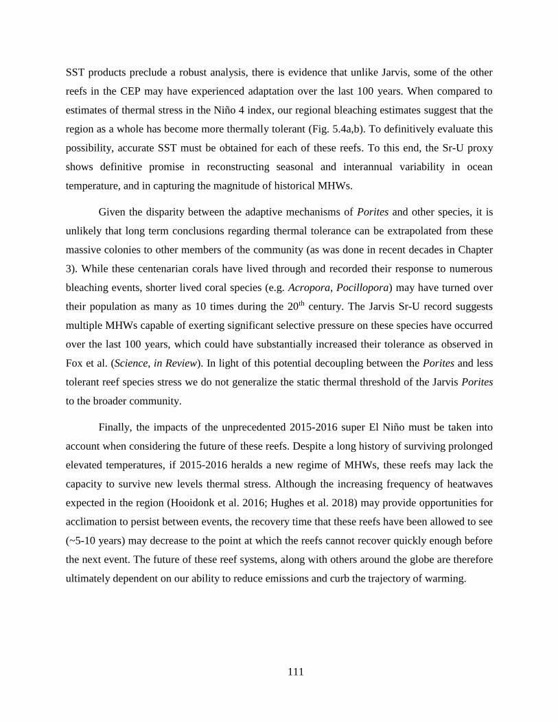
111
SST products preclude a robust analysis, there is evidence that unlike Jarvis, some of the other
reefs in the CEP may have experienced adaptation over the last 100 years. When compared to
estimates of thermal stress in the Niño 4 index, our regional bleaching estimates suggest that the
region as a whole has become more thermally tolerant (Fig. 5.4a,b). To definitively evaluate this
possibility, accurate SST must be obtained for each of these reefs. To this end, the Sr-U proxy
shows definitive promise in reconstructing seasonal and interannual variability in ocean
temperature, and in capturing the magnitude of historical MHWs.
Given the disparity between the adaptive mechanisms of Porites and other species, it is
unlikely that long term conclusions regarding thermal tolerance can be extrapolated from these
massive colonies to other members of the community (as was done in recent decades in Chapter
3). While these centenarian corals have lived through and recorded their response to numerous
bleaching events, shorter lived coral species (e.g. Acropora, Pocillopora) may have turned over
their population as many as 10 times during the 20th century. The Jarvis Sr-U record suggests
multiple MHWs capable of exerting significant selective pressure on these species have occurred
over the last 100 years, which could have substantially increased their tolerance as observed in
Fox et al. (Science, in Review). In light of this potential decoupling between the Porites and less
tolerant reef species stress we do not generalize the static thermal threshold of the Jarvis Porites
to the broader community.
Finally, the impacts of the unprecedented 2015-2016 super El Niño must be taken into
account when considering the future of these reefs. Despite a long history of surviving prolonged
elevated temperatures, if 2015-2016 heralds a new regime of MHWs, these reefs may lack the
capacity to survive new levels thermal stress. Although the increasing frequency of heatwaves
expected in the region (Hooidonk et al. 2016; Hughes et al. 2018) may provide opportunities for
acclimation to persist between events, the recovery time that these reefs have been allowed to see
(~5-10 years) may decrease to the point at which the reefs cannot recover quickly enough before
the next event. The future of these reef systems, along with others around the globe are therefore
ultimately dependent on our ability to reduce emissions and curb the trajectory of warming.
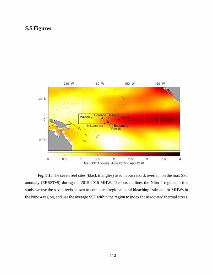
112
5.5 Figures
Fig. 5.1. The seven reef sites (black triangles) used in our record, overlain on the max SST
anomaly (ERSSTv5) during the 2015-2016 MHW. The box outlines the Niño 4 region. In this
study we use the seven reefs shown to compute a regional coral bleaching estimate for MHWs in
the Niño 4 region, and use the average SST within the region to index the associated thermal stress.
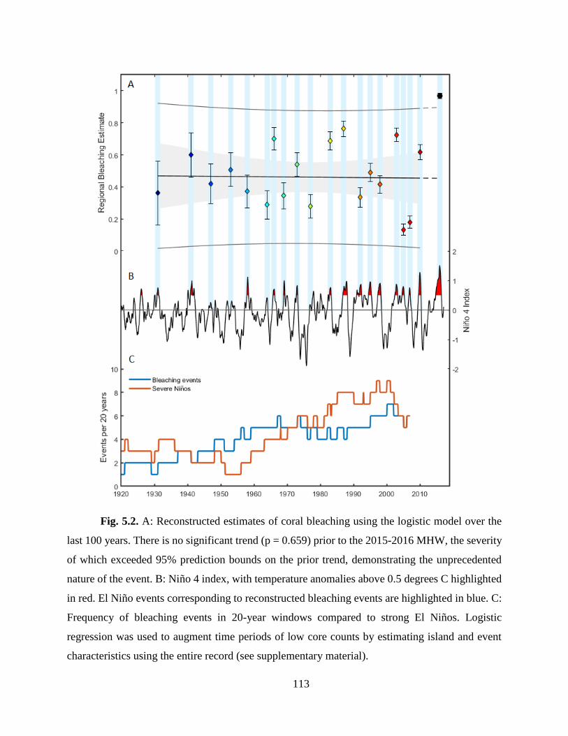
113
Fig. 5.2. A: Reconstructed estimates of coral bleaching using the logistic model over the
last 100 years. There is no significant trend (p = 0.659) prior to the 2015-2016 MHW, the severity
of which exceeded 95% prediction bounds on the prior trend, demonstrating the unprecedented
nature of the event. B: Niño 4 index, with temperature anomalies above 0.5 degrees C highlighted
in red. El Niño events corresponding to reconstructed bleaching events are highlighted in blue. C:
Frequency of bleaching events in 20-year windows compared to strong El Niños. Logistic
regression was used to augment time periods of low core counts by estimating island and event
characteristics using the entire record (see supplementary material).
114
Fig. 5.3. Monthly Sr-U reconstruction of SST at Jarvis island (from core J018). The Sr-U (green)
has been aligned with the SST axis using the calibration presented in chapter 4. The adjusted
HadISST (black) has been binned in the same manner as the Sr-U. Agreement between the two
records is high during the satellite era (top panel), however discrepancies are increasingly observed
moving back in the record, highlighting the uncertainties in the instrumental record pre-satellite.
R2 = 0.72
R2 = 0.62
R2 = 0.55
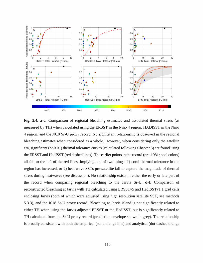
115
Fig. 5.4. a-c: Comparison of regional bleaching estimates and associated thermal stress (as
measured by TH) when calculated using the ERSST in the Nino 4 region, HADISST in the Nino
4 region, and the J018 Sr-U proxy record. No significant relationship is observed in the regional
bleaching estimates when considered as a whole. However, when considering only the satellite
era, significant (p<0.01) thermal tolerance curves (calculated following Chapter 3) are found using
the ERSST and HadISST (red dashed lines). The earlier points in the record (pre-1981; cool colors)
all fall to the left of the red lines, implying one of two things: 1) coral thermal tolerance in the
region has increased, or 2) heat wave SSTs pre-satellite fail to capture the magnitude of thermal
stress during heatwaves (see discussion). No relationship exists in either the early or late part of
the record when comparing regional bleaching to the Jarvis Sr-U. d-f: Comparison of
reconstructed bleaching at Jarvis with TH calculated using ERSSTv5 and HadISSTv1.1 grid cells
enclosing Jarvis (both of which were adjusted using high resolution satellite SST, see methods
5.3.3), and the J018 Sr-U proxy record. Bleaching at Jarvis island is not significantly related to
either TH when using the Jarvis-adjusted ERSST or the HadISST, but is significantly related to
TH calculated from the Sr-U proxy record (prediction envelope shown in grey). The relationship
is broadly consistent with both the empirical (solid orange line) and analytical (dot-dashed orange
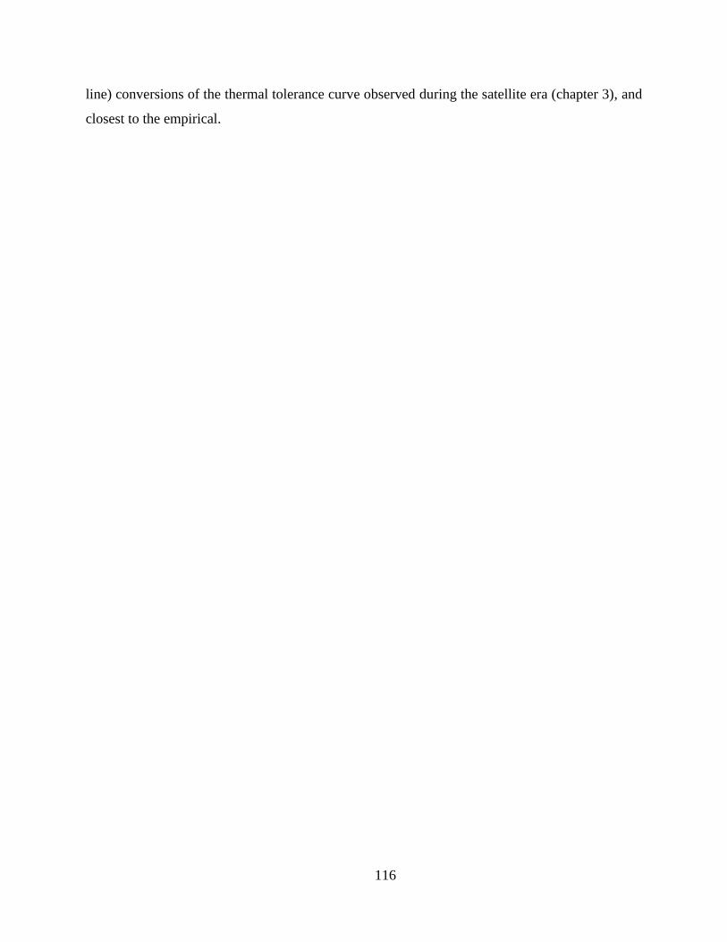
116
line) conversions of the thermal tolerance curve observed during the satellite era (chapter 3), and
closest to the empirical.
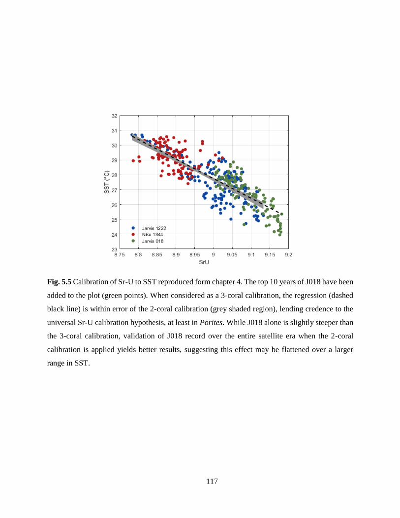
117
Fig. 5.5 Calibration of Sr-U to SST reproduced form chapter 4. The top 10 years of J018 have been
added to the plot (green points). When considered as a 3-coral calibration, the regression (dashed
black line) is within error of the 2-coral calibration (grey shaded region), lending credence to the
universal Sr-U calibration hypothesis, at least in Porites. While J018 alone is slightly steeper than
the 3-coral calibration, validation of J018 record over the entire satellite era when the 2-coral
calibration is applied yields better results, suggesting this effect may be flattened over a larger
range in SST.
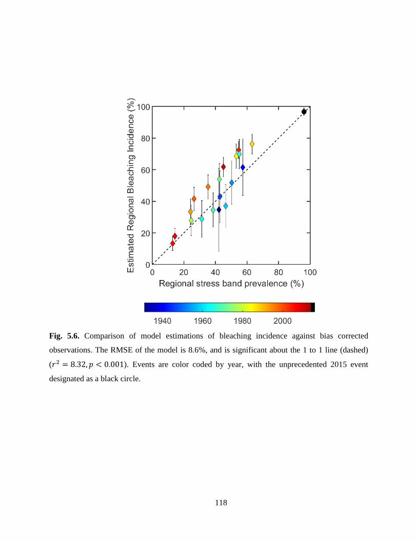
118
Fig. 5.6. Comparison of model estimations of bleaching incidence against bias corrected
observations. The RMSE of the model is 8.6%, and is significant about the 1 to 1 line (dashed)
(𝑟2 = 8.32, 𝑝 < 0.001). Events are color coded by year, with the unprecedented 2015 event
designated as a black circle.
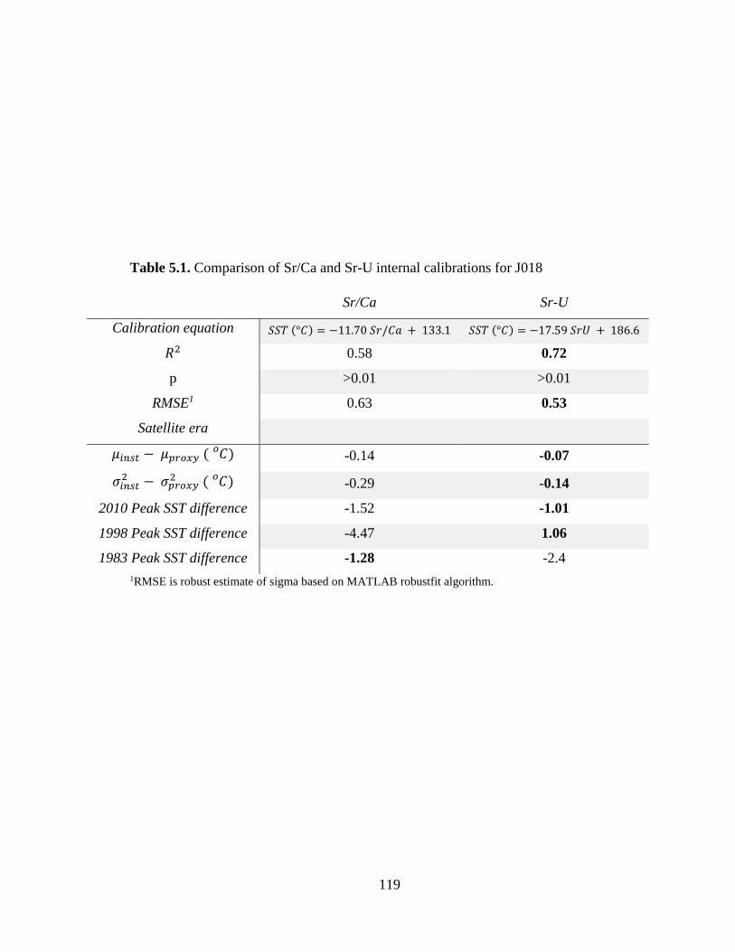
119
Table 5.1. Comparison of Sr/Ca and Sr-U internal calibrations for J018
Sr/Ca Sr-U
Calibration equation 𝑆𝑆𝑇 (°𝐶) = −11.70 𝑆𝑟/𝐶𝑎 + 133.1 𝑆𝑆𝑇 (°𝐶) = −17.59 𝑆𝑟𝑈 + 186.6
𝑅2 0.58 0.72
p >0.01 >0.01
RMSE1 0.63 0.53
Satellite era
𝜇𝑖𝑛𝑠𝑡 − 𝜇𝑝𝑟𝑜𝑥𝑦 ( 𝐶𝑜 ) -0.14 -0.07
𝜎𝑖𝑛𝑠𝑡2 − 𝜎𝑝𝑟𝑜𝑥𝑦
2 ( 𝐶𝑜 ) -0.29 -0.14
2010 Peak SST difference -1.52 -1.01
1998 Peak SST difference -4.47 1.06
1983 Peak SST difference -1.28 -2.4
1RMSE is robust estimate of sigma based on MATLAB robustfit algorithm.
120
5.6 References
Barkley HC, Cohen AL, Brainard RE, Mollica NR, Rivera HE, Drenkard EJ, Young CW, Vargas-
Ángel B, Lohmann GP, Decarlo TM, Alpert AE, Lino KC, Oliver TA, Pietro KR, Luu VH
(2018) Repeat bleaching of a central Pacific coral reef over the past six decades (1960-2016).
Nat Biol Commun
Beck MW, Losada IJ, Menéndez P, Reguero BG, Díaz-Simal P, Fernández F (2018) The global
flood protection savings provided by coral reefs. Nat Commun 9:
Bruno JF, Côté IM, Toth LT (2019) Climate Change, Coral Loss, and the Curious Case of the
Parrotfish Paradigm: Why Don’t Marine Protected Areas Improve Reef Resilience? Ann Rev
Mar Sci 11:
Burns SJ, Godfrey LR, Faina P, McGee D, Hardt B, Ranivoharimanana L, Randrianasy J (2016)
Rapid human-induced landscape transformation in Madagascar at the end of the first
millennium of the Common Era. Quat Sci Rev 134:92–99
Cai W, Borlace S, Lengaigne M, van Rensch P, Collins M, Vecchi G, Timmermann A, Santoso
A, McPhaden MJ, Wu L, England MH, Wang G, Guilyardi E, Jin F-F (2014) Increasing
frequency of extreme El Niño events due to greenhouse warming. Nat Clim Chang 5:1–6
Carré M, Sachs JP, Purca S, Schauer AJ, Braconnot P, Falcón RA, Julien M, Lavallée D (2014)
Holocene history of ENSO variance and asymmetry in the eastern tropical Pacific. Science
(80- ) 345:
Coats S, Karnauskas KB (2017) Are Simulated and Observed Twentieth Century Tropical Pacific
Sea Surface Temperature Trends Significant Relative to Internal Variability? Geophys Res
Lett 44:
DeCarlo TM, Harrison HB, Gajdzik L, Alaguarda D, Rodolfo-metalpa R, Olivo JD, Liu G,
Patalwala D, Mcculloch MT (2019) Acclimatization of massive reef-building corals to
consecutive heatwaves. Proc R Soc B 286:
Donner SD, Rickbeil GJM, Heron SF (2017) A new, high-resolution global mass coral bleaching
database. PLoS One 12:1–17
121
Ferrario F, Beck MW, Storlazzi CD, Micheli F, Shepard CC, Airoldi L (2014) The effectiveness
of coral reefs for coastal hazard risk reduction and adaptation. Nat Commun 5:3794
Fisher R, O’Leary RA, Low-Choy S, Mengersen K, Knowlton N, Brainard RE, Caley MJ (2014)
Species Richness on Coral Reefs and the Pursuit of Convergent Global Estimates. Curr Biol
25:500–505
Frölicher TL, Fischer EM, Gruber N (2018) Marine heatwaves under global warming. Nature
560:360–364
Gleeson MW, Strong AE (1995) Applying MCSST to coral reef bleaching. Adv Sp Res 16:151–
154
Hoegh-Guldberg O (1999) Climate Change, coral bleaching and the future of the world’ s coral
reefs. Ove Hoegh-Guldberg. Mar Freshw Res 50:839–866
van Hooidonk R, Huber M (2009) Quantifying the quality of coral bleaching predictions. Coral
Reefs 28:579–587
Hooidonk R Van, Maynard J, Tamelander J, Gove J (2016) Local-scale projections of coral reef
futures and implications of the Paris Agreement. Nat Publ Gr 1–8
van Hooidonk R, Maynard J, Tamelander J, Gove J, Ahmadia G, Raymundo L, Williams G, Heron
SF, Planes S, Hooidonk R Van, Maynard J, Tamelander J, Gove J (2016) Local-scale
projections of coral reef futures and implications of the Paris Agreement. Sci Rep 6:39666
Hughes TP, Anderson KD, Connolly SR, Heron SF, Kerry JT, Lough JM, Baird AH, Baum JK,
Berumen ML, Bridge TC, Claar DC (2018) Spatial and temporal patterns of mass bleaching
of corals in the Anthropocene. Science (80- ) 359:80–83
Hughes TP, Kerry JT, Álvarez-Noriega M, Álvarez-Romero JG, Anderson KD, Baird AH,
Babcock RC, Beger M, Bellwood DR, Berkelmans R, Bridge TC, Butler IR, Byrne M, Cantin
NE, Comeau S, Connolly SR, Cumming GS, Dalton SJ, Diaz-Pulido G, Eakin CM, Figueira
WF, Gilmour JP, Harrison HB, Heron SF, Hoey AS, Hobbs J-PA, Hoogenboom MO,
Kennedy E V., Kuo C, Lough JM, Lowe RJ, Liu G, McCulloch MT, Malcolm HA,
McWilliam MJ, Pandolfi JM, Pears RJ, Pratchett MS, Schoepf V, Simpson T, Skirving WJ,
Sommer B, Torda G, Wachenfeld DR, Willis BL, Wilson SK (2017) Global warming and
122
recurrent mass bleaching of corals. Nature 543:373–377
Kennedy JJ, Rayner NA, Smith RO, Parker DE, Saunby M (2011) Reassessing biases and other
uncertainties in sea-surface temperature observations measured in situ since 1850 , part 1 :
measurement and sampling uncertainties. J Geophys Res 116:
Klepac CN, Barshis DJ (2020) Reduced thermal tolerance of massive coral species in a highly
variable environment: Reduced heat tolerance of massive corals. Proc R Soc B Biol Sci
287:19–21
Logan CA, Dunne JP, Eakin CM, Donner SD (2014) Incorporating adaptive responses into future
projections of coral bleaching. Glob Chang Biol 20:125–139
Mcclanahan TR, Darling ES, Maina JM, Muthiga NA, Stéphanie D, Jupiter SD, Arthur R, Wilson
SK, Mangubhai S, Nand Y, Ussi AM, Humphries AT, Patankar VJ, Guillaume MMM, Keith
SA, Shedrawi G, Julius P, Grimsditch G, Ndagala J, Leblond J (2019) Temperature patterns
and mechanisms influencing coral bleaching during the 2016 El Niño. Nat Clim Chang 9:
Mollica NR, Cohen AL, Alpert AE, Barkley HC, Brainard RE, Carilli JE, Decarlo TM, Drenkard
EJ, Lohmann P, Mangubhai S (2019) Skeletal records of bleaching reveal different thermal
thresholds of Pacific coral reef assemblages. Coral Reefs
Obura D, Mangubhai S (2011) Coral mortality associated with thermal fluctuations in the Phoenix
Islands, 2002-2005. Coral Reefs 30:607–619
Oliver JK, Berkelmans R, Eakin CM (2018) Coral Bleaching in Space and Time. In: van Oppen
M.J.H., Lough J.M. (eds) Coral Bleaching. Springer, Cham,
Oliver TA, Palumbi SR (2011) Do fluctuating temperature environments elevate coral thermal
tolerance? Coral Reefs 30:429–440
Palumbi SR, Barshis DJ, Bay R a (2014) Mechanisms of reef coral resistance to future climate
change. Science (80- ) 344:895–898
Safaie A, Silbiger NJ, McClanahan TR, Pawlak G, Barshis DJ, Hench JL, Rogers JS, Williams
GJ, Davis KA (2018) High frequency temperature variability reduces the risk of coral
bleaching. Nat Commun 9:1–12
123
Selig ER, Bruno JF (2010) A Global Analysis of the Effectiveness of Marine Protected Areas in
Preventing Coral Loss. PLoS One 5:
Wilkinson C (2004) Status of Coral Reefs of the World. Australian Institute of Marine Science,
Townsville, MC
Van Woesik R, Houk P, Isechal AL, Idechong JW, Victor S, Golbuu Y (2012) Climate-change
refugia in the sheltered bays of Palau: Analogs of future reefs. Ecol Evol 2:2474–2484
Xu Y, Hu A (2018) How would the Twenty-First-Century warming influence pacific decadal
variability and its connection to North American Rainfall: Assessment based on a revised
procedure for the IPO/PDO. J Clim 31:1547–1563

124
125
Chapter 6 – Future Directions
6.1 Introduction
The harsh reality of modern coral reefs is that, like so many of nature’s wonderful
ecosystems, they are under direct and imminent threat from anthropogenic climate change. In the
face of this reality, fatalism and tragic drama have become wide spread among the coral reef
research community, coloring many recent publications with the gloomy air of documenting the
extinction and disappearance of coral reefs as we know them today. While some researchers may
be playing up this gloom and doom sentiment to garner a larger spotlight on the threats (and
thereby generate interest in saving coral reefs), I feel that this is a counterproductive and possibly
dangerous practice for two reasons. First, it obfuscates the truth evident in many recent studies,
including this thesis, that suggest some reefs may have the capacity to survive and even thrive in
a warming world through local environmental mitigations (Wall et al. 2014; DeCarlo et al. 2017)
or adaptive capabilities (Rivera PhD Thesis, 2019; Fox et al., In Review; Oliver and Palumbi 2011;
Mollica et al. 2019). These success stories must be highlighted and pursued such that identification
and protection of climate resilient reefs occurs as soon as possible, as they will provide a bastion
to coral and reef species should the worst projections of warming be realized. Second, coral reef
fatalism often dismisses restoration efforts as inconsequential in the scope of global reef futures in
GCM projections. This has led to a breakdown in communication between coral reef managers
and scientists, which in turn has resulted in a significant proportion of coral restoration work being
undertaken with little or no scientific input or detailed monitoring (Bostrom Einarsson et al., 2020).
If we are to make any effort at saving coral reefs and the species therein, there are several
truths that must be acknowledged. Most important of these is that tropical reefs have already lost
over 50-75% of coral cover to bleaching, increased disease outbreaks, sedimentation and nutrient
pollution, and other anthropogenic stressors in only the last 40 years (Bruno et al. 2019). In even
the most optimistic IPCC projections, warming will continue for at least another 20 years, which
means that conditions will worsen. The next truth is that coral reefs have never in their 500-million-
year history been exposed to warming at the rate it is occurring today. Acclimatization and
adaptation strategies that these species may have relied upon in their genetic history may not be
126
capable of handling the steep warming curve and pronounced heat wave events of the 21st century.
So, what does this mean for coral reef conservation? It is likely too late for even dramatic
reductions in global scale carbon output to save the majority of coral reefs. To be effective,
conservation efforts must therefore have two focuses:
1) To identify and protect those reef communities that have the best chance of surviving
21st century warming through demonstrated higher thermal tolerance, local
environmental processes that mitigate heat stress, or historically proven adaptive
capability.
2) To bridge the decades of inescapable warming in the near future by protecting coral
biodiversity through active restoration efforts aimed at preserving endangered coral
species, actively propagating thermally tolerant individuals, and fostering local
community interest and involvement in mutually beneficial reef preservation
These efforts will only be effective in so far as anthropogenic warming is curbed
substantially in the next century, however coral reef optimists have already identified these focuses
and efforts are being made in both directions.
6.2 Identifying and protecting tolerant reefs
At this point, there exists no single definitive test for identifying thermally tolerant or
resilient corals prior to their exposure to extreme heat. The gold standard for such a test would be
1) minimally destructive, 2) easily administered with minimal training, and 3) economically
feasible. The obvious route would be the detection of a genetic marker related to thermal tolerance,
as most genetic tests meet all three criteria. However, the genomic understanding of coral thermal
tolerance is still in its infancy. Studies have shown heat stressed corals change expression of
hundreds of genes (Meyer et al. 2011; Barshis et al. 2013), and while only a fraction of these are
likely to correspond to thermal defense mechanisms, the difference in response of proven
thermally tolerant individuals suggests there is no single ‘thermal tolerance gene,’ but rather tens
of genes working in concert for any hypothesized tolerance strategy (i.e. production of heat shock
proteins, elimination of radicals). Population genetics has recently yielded exciting results in
identifying thermally tolerant corals within the Palauan reef system (Rivera 2019) and across a
latitudinal gradient in the Great Barrier Reef (Dixon et al. 2015) although these approaches are not
127
yet independent of some stress test validation. The use of CRISPR mutagenesis has also shown
recent promise as a tool to evaluate the importance of gene function in coral thermal tolerance, but
has not yet been put to expansive use (Cleves et al. 2020). While a coral genomics tool for
identifying tolerant corals may become viable in the future, current efforts focus on identifying
tolerant corals post stress, either via direct stress testing or after natural marine heatwaves.
In the absence of a genetic assay for thermal tolerance, heat stress experiments are a more
empirical option and have been employed extensively in recent years. One of the more significant
developments towards experimental stress testing is the CBASS (a portable hot box) which can be
used in the field to conduct short-term (i.e. 18 hour to 3 day) bleaching experiments on collected
fragments of coral (Palumbi et al. 2014). This technique offers advantages over more traditional
heat stress experiments in its portability, ease of use, and cost efficiency. CBASS stress testing has
also recently been shown to identify thermally tolerant corals with the same level of accuracy as
long term (i.e. 21 day) experiments (Voolstra et al. 2020). While these results are promising, in
isolating coral test subjects from their natural environment these experiments may omit
environmental factors that influence bleaching susceptibility (i.e. flow regime, light exposure,
nutrient availability). While an in situ experimental setup is not currently feasible, a more accurate
reconstruction of the coral’s natural environment may improve the applicability of this technique.
We can also make use of natural bleaching events to identify thermally tolerant corals. In
this thesis, I identify thermally tolerant coral populations after they have been subjected to repeat
stress using skeletal records of bleaching, i.e. stress bands. By making use of natural marine
heatwaves, skeletal stress bands can be used to recover thermal tolerance information about both
massive corals and the communities around them years to decades after bleaching events.
However, this technique is not without issue – namely it requires both a prolonged history of
thermal stress events to gauge the tolerance of the sampled population, and a significant number
of large Porites (or potentially other massive species) colonies that can be sampled within the
testing area. While data suggest that these massive colonies are representative of the broader
community in the reefs in this study (Fig. 2.2), this may not be the case everywhere. In terms of
meeting the criteria for this ‘gold standard’ test, current detection methods for stress bands are
costly (requiring CT scanning) and more destructive than tissue biopsy. Future development of the
128
proxy should look towards an in-situ method of stress band detection, perhaps through the use of
acoustic or nuclear instruments common in borehole logging.
Improvements to each of these techniques could lead to one or more becoming the gold
standard of detecting coral thermal tolerance, however all require sampling on a colony scale
making the logistics of their application across the hundreds of thousands of km2 that comprise the
world’s reefs infeasible. Therefore, any in situ assay must be paired with the capability of remotely
identifying likely candidates for thermal tolerance. In order to identify potential climate tolerant
reef communities from afar, our best resort is high resolution hydrodynamic modelling (e.g.
Regional Ocean Modeling System, ROMS). Localized reef environments capable of promoting
thermal tolerance (e.g. long residence times leading to chronically high water temperatures or
shallow reef substrate subject to high temperature variability) are a result of complex
geomorphology on scales difficult to resolve with even high-resolution (4km) satellite SST. Given
accurate bathymetry, ROMS nested in coarser regional datasets have been shown to provide
accurate temperatures across even complex reef environments on the scale of meters (REFS). The
use of ROMS in identifying possible thermally tolerant communities is also in its infancy, however
its potential to inform the selection of field sites for tolerance assay is significant. Pairing these
two methods will allow us to quickly and efficiently identify reef communities that have the best
chance of surviving 21st century warming.
6.3 Active restoration efforts
If these efforts are successful, it is critical that scientific involvement in the conservation
process not stop at this point and simply turn over the responsibility to local governments and
stakeholders. Over the last few decades, coral restoration has begun to gain both publicity and
support, however efforts have suffered from two key issues: 1) poor design of many projects due
to insufficient scientific foundation (e.g. lack of experimental control, poorly chosen reference
systems), and 2) lack of consistent monitoring of existing projects, with little to no reporting on
the long-term success or failure (Bostrom-Einarsson et al. 2020). These challenges have led
resource managers to be reluctant in undertaking large and long-term restoration projects, and have
prevented the development of scalable restoration efforts. Greater scientific involvement in
restoration efforts will serve to close this gap by developing more efficient and longer lasting
129
restoration methods. Several such techniques have already been developed, but scalability remains
the biggest scientific impediment to coral reef restoration.
Coral gardening was among the first developments in reef restoration, adding a nursery
phase to transplant efforts. This process aims at increasing transplant success by allowing outplants
to grow to an optimal size threshold, and also allows nurseries to maintain a standing stock of coral
from which outplants can be made. However, while some studies report high rates of survival
(Putchim et al. 2008), a recent review of transplant studies concluded that on average gardened
corals had only a 2% higher survival rate than direct transplants (Bostrom-Einarsson et al. 2020).
This disparity between anticipated result and observed outcome highlights a lack of robust
experimental validation. Future efforts in coral gardening could be improved by optimizing
survivability in several ways. Targeting thermally tolerant coral individuals for replication
increases the likelihood of restoration efforts lasting through future bleaching events. Also, pairing
outplanting with substrate stabilization techniques has been shown to enhance coral recruitment
significantly (Lindahl 2003).
Gardening has also been primarily limited to fast growing branching coral genera, and
while propagation of these genera is easier as they are more amenable to fragmentation, these same
genera are among the least thermally tolerant (Loya et al. 2001). To both maintain biodiversity and
stability of reef systems through anthropogenic warming, the massive slow growing species (e.g.
Porites, Montastrea) that form the backbone of reef construction must be preserved. Micro-
fragmentation, a recent technique developed to accelerate the propagation of polyps in massive
corals, has shown incredible promise in both the growth and survival of gardened outplants
(Forsman et al. 2015). Using this method, new coral can be ‘re-skinned’ over dead colonies, not
only restoring live coral cover to a reef but substantially reducing deterioration of substrate.
However, while promising, this technique also suffers from a lack of scalability. To be attractive
to coral reef managers, local scale efforts in outplanting should focus on 1) identifying and
propagating thermally tolerant corals to maximize survivability, and 2) focus on reef areas less
susceptible to local stressors (i.e. pristine or protected areas) and global stressors (i.e. heat
mitigating hydrodynamics, low rates of warming).
One restoration technique that shows promise in terms of scalability is larval enhancement.
This method seeks to increase rates of coral fertilization by collecting or rearing larvae and
130
distributing them onto the reef either directly or via settlement structures. Two methods have been
utilized to date; one study harvested embryos reared in a coral nursery, and settled them onto
concrete tetrapods which were then scattered onto the reef (Chamberland et al. 2017). The second
study reared collected embryos in holding tanks on the reef, after which the larvae were released
into enclosures over target substrate (Heyward et al. 2002). While both efforts were significantly
faster than outplanting, they observed lower rates of success. Nevertheless, larval enhancement
shows the most promise of current restorations in scaling to the thousands of square kilometers of
reef area threatened by ocean warming. Further development of this technique in terms of both
survivability of recruits and dispersal efficiency could potentially have massive results. If collected
from a sufficiently genetically diverse population, recruits placed via larval enhancement will also
be less sensitive to disease, a problem inherent in propagation-based techniques. And, like other
methods of coral planting, larval enhancement would also benefit from identifying and replicating
thermally tolerant individuals.
6.4 Conclusions
The most important steps scientific advancement can make toward helping coral reefs
survive anthropogenic warming are not as passive observers, but as active defenders. Identifying,
protecting, nurturing reef communities that are capable of surviving 21st century warming is central
to this effort. Considerable scientific effort has been made in this direction, but improvements can
still be made. In the face of the inescapable warming projected over the coming decades, active
restoration efforts must be employed to maintain both the abundance and biodiversity of these
tolerant reef systems. While restoration techniques are not yet viable on the scale necessary, recent
advances in these techniques have improved their success rate and potential use over large spatial
scales. However, even with a concerted effort to give these reefs the best chance possible in
surviving warming, all corals have a limit to their thermal tolerance. Without the abatement of
anthropogenic warming through the reduction of fossil fuel emissions, these efforts will be in vain.
131
6.5 References
Barshis DJ, Ladner JT, Oliver TA, Seneca FO, Traylor-Knowles N, Palumbi SR (2013) Genomic
basis for coral resilience to climate change. Proc Natl Acad Sci 110:1387–1392
Bostrom-Einarsson L, Babcock RC, Baryaktarov E, Ceccarelli D, Cook N, Ferse S, Hancock B,
Harrison P, Hein M, Shaver E, Smith A, Suggett D, Stewart-Sinclair P, Vardi T, McLeod I
(2020) Coral restoration – A systematic review of current methods, successes, failures and
future directions. PLoS One 13:1–24
Bruno JF, Côté IM, Toth LT (2019) Climate Change, Coral Loss, and the Curious Case of the
Parrotfish Paradigm: Why Don’t Marine Protected Areas Improve Reef Resilience? Ann Rev
Mar Sci 11:
Chamberland VF, Petersen D, Guest JR, Petersen U, Brittsan M, Vermeij MJA (2017) New
Seeding Approach Reduces Costs and Time to Outplant Sexually Propagated Corals for Reef
Restoration. Sci Rep 7:1–12
Cleves P, Tinoco A, Bradford J, Perrin D, Bay L, Pringle J (2020) Reduced heat tolerance in a
coral carrying CRISPR-induced mutations in the gene for a heat-shock transcription factor.
Proc Natl Acad Sci USA 117:28899–28905
DeCarlo TM, Cohen AL, Wong GTF, Davis KA, Lohmann P, Soong K (2017) Mass coral
mortality under local amplification of 2 °C ocean warming. Sci Rep 7:44586
Dixon G, Davies S, Aglyamova G, Meyer E, Bay L, Matz M (2015) Genomic Determinants of
Coral Heat Tolerance Across Latitudes. Science (80- ) 348:2014–2016
Forsman ZH, Page CA, Toonen RJ, Vaughan D (2015) Growing coral larger and faster: Micro-
colony-fusion as a strategy for accelerating coral cover. PeerJ
Heyward AJ, Smith LD, Rees M, Field SN (2002) Enhancement of coral recruitment by in situ
mass culture of coral larvae. Mar Ecol Prog Ser 230:113–118
Lindahl U (2003) Coral reef rehabilitation through transplantation of staghorn corals: Effects of
artificial stabilization and mechanical damages. Coral Reefs 22:217–223
132
Loya Y, Sakai K, Yamazato K, Nakano Y, Sambali H, Van Woesik R (2001) Coral bleaching: The
winners and the losers. Ecol Lett 4:122–131
Meyer E, Aglyamova G V., Matz M V. (2011) Profiling gene expression responses of coral larvae
(Acropora millepora) to elevated temperature and settlement inducers using a novel RNA-
Seq procedure. Mol Ecol 20:3599–3616
Mollica NR, Cohen AL, Alpert AE, Barkley HC, Brainard RE, Carilli JE, Decarlo TM, Drenkard
EJ, Lohmann P, Mangubhai S (2019) Skeletal records of bleaching reveal different thermal
thresholds of Pacific coral reef assemblages. Coral Reefs
Oliver TA, Palumbi SR (2011) Do fluctuating temperature environments elevate coral thermal
tolerance? Coral Reefs 30:429–440
Palumbi SR, Barshis DJ, Bay R a (2014) Mechanisms of reef coral resistance to future climate
change. Science (80- ) 344:895–898
Putchim L, Thongtham N, Hewett A, Chansang H (2008) Survival and growth of Acropora spp.
in mid-water nursery and after transplantation at Phi Phi Islands , Andaman Sea , Thailand.
11th Int Coral Reef Symp Ft Lauderdale, Florida 1258–1261
Rivera HE (2019) Genetic connectivity, adaptation, and phenotypic plasticity of corals and
anemones under thermal stress. Dr Thesis
Voolstra CR, Buitrago-López C, Perna G, Cárdenas A, Hume BCC, Rädecker N, Barshis DJ
(2020) Standardized short-term acute heat stress assays resolve historical differences in coral
thermotolerance across microhabitat reef sites. Glob Chang Biol 26:4328–4343
Wall M, Wall M, Putchim L, Schmidt GM, Jantzen C, Khokiattiwong S (2014) Large-amplitude
internal waves benefit corals during thermal stress Large-amplitude internal waves benefit
corals during thermal stress. Proc R Soc B
133
Appendix A2 – Supplementary text, figures,
and data for chapter 2
A2.1 Correlation between coral skeletal density and RECM on the
seasonal scale
Coral skeletal density shows a significant correlation (p < 0.05) with RECM on the seasonal
scale in 5 out of the 9 cores analyzed in this study, consistent with the control of the skeletal
thickening rate on skeletal density (Fig. A2.3). Seasonal RECM was estimated following the same
method as the annual RECM (Methods), except that seasonal seawater temperatures were estimated
at the same resolution as the boron isotope measurements (e.g. 6-8 samples per year). The rate of
skeletal extension was assumed constant throughout the year.
Note, the absence of such correlation in some cores can be due to improper alignment
between the density profile and the sampling track for boron isotope measurements. Density
determined by CT scanning represents average density across all continuous polyps in the core,
while boron isotope sampling was conducted along a single polyp. This misalignment issue can be
accounted for if certain amount of shift in the density profile is applied. For example, the
correlation between the coral skeletal density and RECM in core Green Island 701 improves
significantly (from p=0.098 to p < 0.001), if a 1mm shift is applied. For other cores, e.g. Saboga
192 and Airai 23, the skeletal density shows minimal annual cyclicity. Accordingly, there are poor
correlation between the coral skeletal density and RECM.
A2.2. Elevation of DIC concentration in coral ECM
Several studies have attempted to quantify the DIC concentrations within the coral ECM
with different geochemical methods. For example, Allison et al. estimated a factor of 1.4 times
elevation of DIC concentrations in Porites coral ECM (Allison et al. 2014), by combining
estimates of ECM pH from δ11B and estimation of ECM CO32- and HCO3
- concentrations from
B/Ca ratios. However, McCulloch et al. recently estimated a much higher elevation (i.e. a factor
of 2.6) of DIC concentration in Porites coral ECM using a similar approach (Holcomb et al. 2016).
134
This difference results mainly from the different ways the two studies used to derive the boron
partition coefficient between seawater and aragonite. McCulloch et al. also suggested the DIC
elevations in coral ECM vary seasonally, with elevation factors fluctuating by 0.74 on average.
However, the annual average DIC elevations estimated from their data are relatively constant,
ranging by 0.20 between years. In a study using the same approach, Comeau et al. found DIC in
the ECM to be elevated by a factor of 1.8 in A. youngei, and 1.7 in P. damicornis (Comeau et al.
2017). Elevation of DIC concentration in coral ECM was also suggested by Furla et al., who
observed that S. pistillata corals growing in calcium and carbon labeled seawater show only about
20~25% of the C14/Ca45 ratio of the surrounding seawater in their skeletons and thus estimated a
DIC elevation factor of ~3 in the their ECM (Furla 2000). In contrast, Cai et al. reconstructed the
full carbonate chemistry of the ECM in O. faveolata, T. reniformis, and A. millepora corals, based
on in situ electrode measurements of ECM pH and CO32- concentrations, and suggest DIC
concentrations in their ECM can be similar to seawater (e.g. an elevation factor of 0.7 to 3.9).
These variations in estimated DIC elevation factors could suggest differences in DIC elevation
among different coral species and individuals.
In this study, we adopt a DIC elevation factor (i.e. α) of 2 and refine this estimation using
a Bayesian statistical approach (See section A2.4). Consideration of seasonal variations in ECM
DIC elevations similar to what suggested by McCulloch et al. does not affect our conclusions (Fig.
A2.3).
A2.3. Porites skeletal growth model
We modeled skeletal growth of Porites corals as a two-step process: daily vertical
extension (E), followed by thickening around the interior to the depth of the tissue layer (Td). Coral
poly is approximated as ring in our model. Each new skeletal element is prescribed a height
equivalent to the daily extension (E) and an initial wall thickness of 𝑤𝑜. Skeletal thickening occurs
throughout the tissue layer, and its rate is controlled by the aragonite precipitation rate in the ECM
(RECM) and decreases with depth in the tissue layer:
𝑅(𝑧) = 𝑅𝐸𝐶𝑀 × 𝑒−
𝜆 × 𝑧(𝑡,𝐸)
𝑇𝑑 [A2.1]
135
where z is the depth at which the skeletal element resides relative to top of the tissue layer
and is a function of time (t) and extension rate (E), R(z) is the thickening rate at depth z, λ is the
decay constant. The wall thickness of polyp ring increase as thickening of skeletal elements
continues:
𝑑𝑤
𝑑𝑡=
𝑅(𝑧)
𝜌𝑎𝑟𝑎𝑔=
𝑅𝐸𝐶𝑀
𝜌𝑎𝑟𝑎𝑔× 𝑒
−𝜆 ×𝑧(𝑡,𝐸)
𝑇𝑑 [A2.2]
where 𝑑𝑤
𝑑𝑡 is the change in wall thickness at a given depth z within the tissue layer due to
thickening, and 𝜌𝑎𝑟𝑎𝑔 is the density of aragonite (i.e. 2.94 g cm-3)(5). The final wall thickness of
the polyp (𝑤𝑓) can then be calculated as:
𝑤𝑓 = 𝑤𝑜 + ∫𝑅𝐸𝐶𝑀
𝜌𝑎𝑟𝑎𝑔× 𝑒
−𝜆 × 𝑧(𝑡,𝐸)
𝑇𝑑 𝑑𝑡𝑡=𝑡𝑓
𝑡=0 [A2.3]
where 𝑑𝑤
𝑑𝑡 is integrated over the entire period for which each skeletal element remains in
the tissue layer (𝑡𝑓). The final density of the skeleton was then calculated based on the fraction of
the ring filled with aragonite (Eq. 3 in the main text).
A2.4. Estimation of model parameters with a Bayesian inference
method
There are limited experimental constraints on several parameters in our skeletal growth
model, including the initial thickness of new skeletal framework (𝑤𝑜), the decline of thickening
rate with depth in the tissue (𝜆), and the DIC elevation within the ECM (α). We estimated these
parameters with a Bayesian inference method. Bayesian inference begins with a prior distribution
for the parameter (or parameters) of interest that reflects prior information. The prior distribution
is then updated with new data via Bayes’ Rule to form the posterior distribution of the parameter
that reflects both prior information and the information contained in the data. A point estimate of
the parameter is then given by its posterior mean and a measure of estimation precision is given
by its posterior standard deviation.
136
A2.4.1 Constructing prior distributions for free parameters
𝒘𝒐. The new skeletal framework in our model is analogous to the early mineralization
zones (EMZ) observed in Porites skeletons, which are thought to represent rapid initial growth at
the apex of skeletal elements every 24 hours (Cuif and Dauphin 2005; Northdruft and Webb 2007;
Shirai et al. 2012). Here we consider the EMZ to consist of the dark, organic rich, centers of
calcification and the immediately associated fibers (Fig. A2.2). As 𝑤𝑜 is a nonzero positive
quantity, we adopt a log-normal distribution prior for 𝑤𝑜, with a mean and variance of the
experimentally determined sizes of EMZ (i.e. 35.4 μm, 29.6 μm respectively).
𝝀. The decrease of skeletal thickening rate within the tissue layer of Porites is a poorly
understood process. Barnes and Lough first described this feature in Porites coral cores from the
Great Barrier Reef, noting a high amount of skeletal thickening near the colony surface and then
rapid decrease toward the base of the tissue layer (Barnes and Lough 1993). Similar trends have
later also been observed in Indo-Pacific Porites (Gagan et al. 2012). Following previous modeling
studies (Elman 1991; Taylor et al. 1993), we simulate this decrease as an exponential function with
decay constant 𝜆. However, to our knowledge there have been no quantitative estimates of 𝜆. We
therefore adopt a uniform prior distribution for 𝜆 greater than zero.
𝛂. As discussed in section A2.2, existing estimates for the DIC elevation factor in the ECM
(α) vary significantly among different species and methods. We chose to adopt a log-normal
distribution prior for α with a mean 2.0. To reflect the large differences between studies, a
distribution with standard deviation 2 times that of the log of observed experimental values in
(Mcculloch et al. 2017) (i.e. 0.14) was used.
A2.4.2 Evaluating likelihood and posterior distributions of parameter estimates
A joint prior distribution was assembled to reflect the combined probability of all possible
combinations of these three parameters. We then simulate the density of each core from this study
using all possible combinations of parameters described by the joint prior based on our skeletal
growth model. The likelihood of each combination of parameters was evaluated by comparing our
measured densities with the associated model predictions assuming normally distributed sample
error. This joint likelihood function was then used to update the prior via Bayes’ theorem to form
the posterior (Fig. A2.4a-c). A univariate distribution for each parameter was generated from the
joint posterior by evaluating the maximum probability of the other two parameters for any given
137
value. For example, for each possible α = αi, there exists a two-parameter posterior of 𝑑𝑤1 and λ.
The maximum of this 2D distribution was taken to be the probability of αi, p(αi). This was then
repeated for the other two parameters.
In the end, our Bayesian inference method yields the following estimates of each
parameter: 𝑤𝑜 = 59 −24+23 𝜇𝑚, λ = 12.8 −6.2
+11.9, and α = 2.05 −0.38+0.39 (2 ).
A2.4.3 Validating Bayesian estimated parameters using skeletal density profiles
We examined skeletal density profiles from within the tissue layer of 5 cores collected in
this study (those that were not damaged at the top). A composite profile was then produced by
normalizing the individual profiles to their respective tissue thicknesses (Td) and fit with an
exponential regression for which a 95% confidence interval was calculated (Fig. A2.4d). We then
employ our Porites skeletal growth model to generate predictions of the density profile within the
tissue layer, using the normalized Td and average 𝑟𝑜, E, and RECM from the five cores. Because the
model predicted curve falls within the 95% confidence interval of the exponential fit, and replicates
the normalized density profile reasonably well, we accept these parameters as satisfactory for our
predictions.
A2.5. Sensitivity of model predicted density to different model
parameters
While RECM plays a significant role in skeletal density in our model, other measured model
parameters (ro, Td, E) also exert significant controls, as do the estimated model parameters (𝑤𝑜, λ,
Fig. A2.5). In brief, predicted density is directly proportional to RECM, Td, 𝑤𝑜, and λ (e.g. an
increase in λ leads to a higher predicted density), while it is inversely proportional to ro and E. We
evaluate below the sensitivity of the model predicted density to each parameter, by individually
varying each parameter by up to 50% while holding all the other parameters constant at the mean
value observed in our cores.
RECM: As discussed in the main text, the model predicted density is sensitive to RECM,
yielding a 0.54% change in density for every 1% change in RECM. RECM is most sensitive to
temperature; in the context of 20th century climate change, we project a mean temperature rise of
2.5 degrees at reef locations (based on CESM-BGC output), which corresponds to an 83% increase
138
in RECM. In comparison, CESM-BGC projected change in seawater pH (i.e. -0.3 units) and in DIC
(i.e. 120 µmol/kg) produces smaller changes in RECM, -32% and 11% respectively.
ro: Among all the model parameters, ro has the strongest effect on the model predicted
density, producing a -1% change in density for every 1% change in ro. ro varies among different
coral species, and is often used for identifying coral taxonomy (Veron and Stafford-Smith 2000).
Little is known about how ro changes with environmental factors. Tambutté et al. (Tambutté et al.
2015) observed that calyx radii of S. pistillata growing in low pH seawater (i.e pH = 7.2) increased
by over 50% compared to those in normal seawater. Note, however, this increase was based on
measurement of the interior radii of the calyx, and so is not directly comparable to ro in our model.
In the Andaman Sea, Tanzil et al. (Tanzil et al. 2009) found that the average cross section areas of
Porites polyps varied significantly between reefs (with a standard deviation of ~10%), but there
was no consistent trend through time.
E: The model predicted density is also sensitive to changes in E, producing -0.30% in
density for every 1% change in E. Many environmental factors are thought to affect the rate of
coral extension, particularly temperature and irradiance. Some studies suggest coral extension
increases linearly with sea surface temperature (Nie et al. 1997; Lough and Barnes 2000), while
others show sharp decreases in coral extension above a threshold temperature or after bleaching
events (Cooper et al. 2008; De’ath et al. 2009; Cantin et al. 2010; Hetzinger et al. 2016). Coral
extension has also been found to decrease with lower irradiance (Baker and Weber 1975; Huston
1985), but is relatively insensitive to ocean acidification (Fabricius et al. 2011; Barkley et al. 2015;
Tambutté et al. 2015).
Td: The model is least sensitive to changes in Td, resulting in 0.28% change in density for
every 1% change in Td. Changes in Td are generally thought to be related to nutrient concentrations
in seawater, and are not affected by ocean acidification (Fabricius et al. 2011; Barkley et al. 2015).
𝒘𝒐: The model is less sensitive to changes in 𝑤𝑜 than RECM, resulting in 0.36% change in
density for every 1% change in 𝑤𝑜. 𝑤𝑜 is thought to be a phenotypic characteristic of Porites; no
evidence has shown a change in EMZ size in response to external stimuli.
𝝀: The model is similarly sensitive to the estimated value of 𝜆 as it is to E, resulting in -
0.31% change in density for every 1% change in 𝜆. As stated above, the rate of decrease in skeletal
139
thickening within the tissue layer is a poorly understood process, and has also not been linked to
any external stimuli.
A2.6. Comparison between model predicted density and measured
density in the existing studies
To enable density predictions, our model requires several input parameters specific to each
coral, including extension rate (E), polyp radius (𝑟𝑜), and tissue thickness (Td). In addition,
seawater carbonate chemistry parameters are needed to estimate RECM. No studies examined in our
model-data comparison reported all of these parameters. When not reported, the values of these
parameters were either adopted from other studies reporting such parameters in the region (e.g. Td
and seawater chemistry) or assumed representative average values for each taxon (e.g. 𝑟𝑜). The
performance of our model is directly related to the uncertainties associated with these measured or
estimated parameters.
Great Barrier Reef: 𝑟𝑜 was not reported for Great Barrier reef cores (Lough and Barnes
2000). But each core was identified at the species level (unlike the Andaman Sea cores). This
allowed for a relatively precise estimation of 𝑟𝑜 (Fig. A2.6b, (Veron and Stafford-Smith 2000)),
which contributes to more satisfactory predictions generated at these locations. For some cores,
there are insufficient in situ measurements about their seawater carbonate chemistry. In these
cases, we used pH, T, S, and DIC output from the CESM-BGC historical run (1900-2005) to
estimate the seawater conditions during time period when density was reported. This could
introduce uncertainties in the estimated RECM, because the physicochemical conditions of the reef
environments can be significantly different from the open ocean conditions (as estimated with
output from the CESM-BGC historical run).
Galapagos: Neither 𝑟𝑜 nor Td were measured for Galapagos corals (28). Instead, we
adopted the mean 𝑟𝑜 values from our cores and the Td (i.e. 6.5mm) estimated from nearby sites
(Wellington et al. 1996; Linsley et al. 1999) in the model predictions. Despite these limitations,
the model predicted density strongly correlates with measured density (p=0.001).
Andaman Sea: Data about the Andaman Sea corals were compiled from two studies
(Tanzil et al. 2009, 2013). 𝑟𝑜 and Td were reported in (Tanzil et al. 2009) but not in (29). The mean
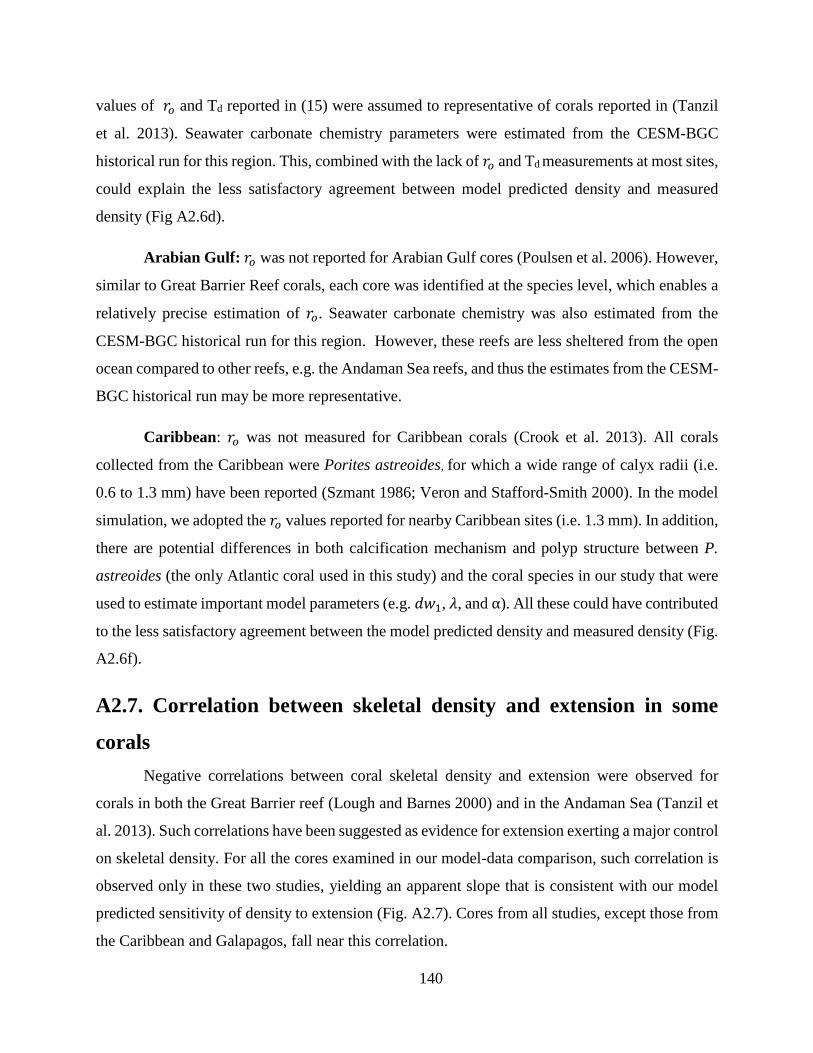
140
values of 𝑟𝑜 and Td reported in (15) were assumed to representative of corals reported in (Tanzil
et al. 2013). Seawater carbonate chemistry parameters were estimated from the CESM-BGC
historical run for this region. This, combined with the lack of 𝑟𝑜 and Td measurements at most sites,
could explain the less satisfactory agreement between model predicted density and measured
density (Fig A2.6d).
Arabian Gulf: 𝑟𝑜 was not reported for Arabian Gulf cores (Poulsen et al. 2006). However,
similar to Great Barrier Reef corals, each core was identified at the species level, which enables a
relatively precise estimation of 𝑟𝑜. Seawater carbonate chemistry was also estimated from the
CESM-BGC historical run for this region. However, these reefs are less sheltered from the open
ocean compared to other reefs, e.g. the Andaman Sea reefs, and thus the estimates from the CESM-
BGC historical run may be more representative.
Caribbean: 𝑟𝑜 was not measured for Caribbean corals (Crook et al. 2013). All corals
collected from the Caribbean were Porites astreoides, for which a wide range of calyx radii (i.e.
0.6 to 1.3 mm) have been reported (Szmant 1986; Veron and Stafford-Smith 2000). In the model
simulation, we adopted the 𝑟𝑜 values reported for nearby Caribbean sites (i.e. 1.3 mm). In addition,
there are potential differences in both calcification mechanism and polyp structure between P.
astreoides (the only Atlantic coral used in this study) and the coral species in our study that were
used to estimate important model parameters (e.g. 𝑑𝑤1, 𝜆, and α). All these could have contributed
to the less satisfactory agreement between the model predicted density and measured density (Fig.
A2.6f).
A2.7. Correlation between skeletal density and extension in some
corals
Negative correlations between coral skeletal density and extension were observed for
corals in both the Great Barrier reef (Lough and Barnes 2000) and in the Andaman Sea (Tanzil et
al. 2013). Such correlations have been suggested as evidence for extension exerting a major control
on skeletal density. For all the cores examined in our model-data comparison, such correlation is
observed only in these two studies, yielding an apparent slope that is consistent with our model
predicted sensitivity of density to extension (Fig. A2.7). Cores from all studies, except those from
the Caribbean and Galapagos, fall near this correlation.
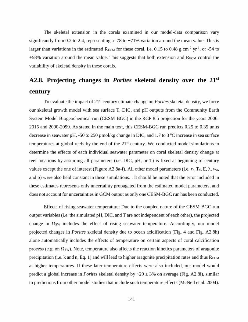
141
The skeletal extension in the corals examined in our model-data comparison vary
significantly from 0.2 to 2.4, representing a -78 to +71% variation around the mean value. This is
larger than variations in the estimated RECM for these coral, i.e. 0.15 to 0.48 g cm-2 yr-1, or -54 to
+58% variation around the mean value. This suggests that both extension and RECM control the
variability of skeletal density in these corals.
A2.8. Projecting changes in Porites skeletal density over the 21st
century
To evaluate the impact of 21st century climate change on Porites skeletal density, we force
our skeletal growth model with sea surface T, DIC, and pH outputs from the Community Earth
System Model Biogeochemical run (CESM-BGC) in the RCP 8.5 projection for the years 2006-
2015 and 2090-2099. As stated in the main text, this CESM-BGC run predicts 0.25 to 0.35 units
decrease in seawater pH, -50 to 250 µmol/kg change in DIC, and 1.7 to 3 oC increase in sea surface
temperatures at global reefs by the end of the 21st century. We conducted model simulations to
determine the effects of each individual seawater parameter on coral skeletal density change at
reef locations by assuming all parameters (i.e. DIC, pH, or T) is fixed at beginning of century
values except the one of interest (Figure A2.8a-f). All other model parameters (i.e. ro, Td, E, λ, wo,
and α) were also held constant in these simulations. . It should be noted that the error included in
these estimates represents only uncertainty propagated from the estimated model parameters, and
does not account for uncertainties in GCM output as only one CESM-BGC run has been conducted.
Effects of rising seawater temperature: Due to the coupled nature of the CESM-BGC run
output variables (i.e. the simulated pH, DIC, and T are not independent of each other), the projected
change in ΩSW includes the effect of rising seawater temperature. Accordingly, our model
projected changes in Porites skeletal density due to ocean acidification (Fig. 4 and Fig. A2.8h)
alone automatically includes the effects of temperature on certain aspects of coral calcification
process (e.g. on ΩSW). Note, temperature also affects the reaction kinetics parameters of aragonite
precipitation (i.e. k and n, Eq. 1) and will lead to higher aragonite precipitation rates and thus RECM
at higher temperatures. If these later temperature effects were also included, our model would
predict a global increase in Porites skeletal density by ~29 ± 3% on average (Fig. A2.8i), similar
to predictions from other model studies that include such temperature effects (McNeil et al. 2004).
142
However, there are large uncertainties regarding how rising sea surface temperatures will
affect coral calcification, particularly related to its effects on zooxanthelae photosynthesis and
coral bleaching (Coles and Jokiel 1977; Warner et al. 1996; Hooidonk et al. 2016). We therefore,
as stated in the main text, focus on evaluating the changes in Porites skeletal density derived solely
from ocean acidification in our model projections and hold the kinetics parameters of aragonite
precipitation constant as calculated at the beginning of century temperatures.
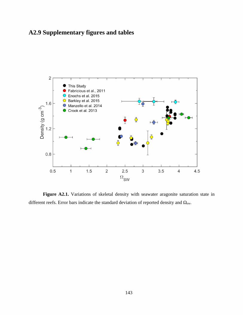
143
A2.9 Supplementary figures and tables
Figure A2.1. Variations of skeletal density with seawater aragonite saturation state in
different reefs. Error bars indicate the standard deviation of reported density and Ωsw.
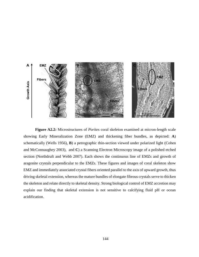
144
Figure A2.2: Microstructures of Porites coral skeleton examined at micron-length scale
showing Early Mineralization Zone (EMZ) and thickening fiber bundles, as depicted: A)
schematically (Wells 1956), B) a petrographic thin-section viewed under polarized light (Cohen
and McConnaughey 2003), and C) a Scanning Electron Microscopy image of a polished etched
section (Northdruft and Webb 2007). Each shows the continuous line of EMZs and growth of
aragonite crystals perpendicular to the EMZs. These figures and images of coral skeleton show
EMZ and immediately associated crystal fibers oriented parallel to the axis of upward growth, thus
driving skeletal extension, whereas the mature bundles of elongate fibrous crystals serve to thicken
the skeleton and relate directly to skeletal density. Strong biological control of EMZ accretion may
explain our finding that skeletal extension is not sensitive to calcifying fluid pH or ocean
acidification.
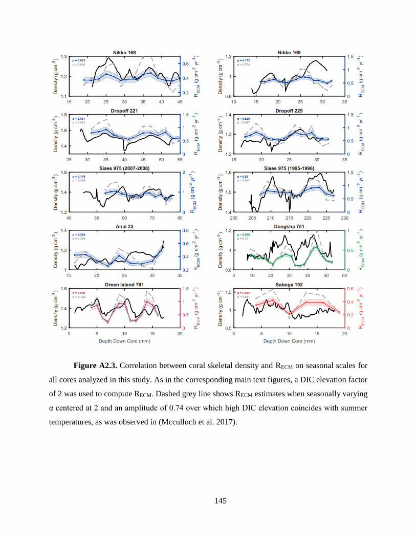
145
Figure A2.3. Correlation between coral skeletal density and RECM on seasonal scales for
all cores analyzed in this study. As in the corresponding main text figures, a DIC elevation factor
of 2 was used to compute RECM. Dashed grey line shows RECM estimates when seasonally varying
α centered at 2 and an amplitude of 0.74 over which high DIC elevation coincides with summer
temperatures, as was observed in (Mcculloch et al. 2017).
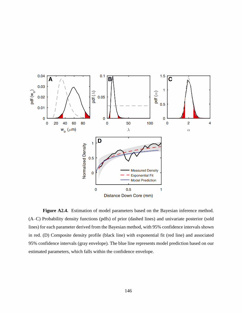
146
Figure A2.4. Estimation of model parameters based on the Bayesian inference method.
(A–C) Probability density functions (pdfs) of prior (dashed lines) and univariate posterior (sold
lines) for each parameter derived from the Bayesian method, with 95% confidence intervals shown
in red. (D) Composite density profile (black line) with exponential fit (red line) and associated
95% confidence intervals (gray envelope). The blue line represents model prediction based on our
estimated parameters, which falls within the confidence envelope.
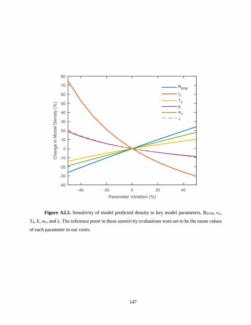
147
Figure A2.5. Sensitivity of model predicted density to key model parameters, RECM, ro,,
Td, E, wo, and λ. The reference point in these sensitivity evaluations were set to be the mean values
of each parameter in our cores.
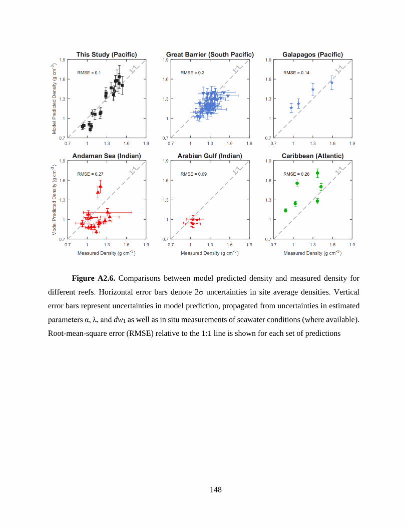
148
Figure A2.6. Comparisons between model predicted density and measured density for
different reefs. Horizontal error bars denote 2σ uncertainties in site average densities. Vertical
error bars represent uncertainties in model prediction, propagated from uncertainties in estimated
parameters α, λ, and dw1 as well as in situ measurements of seawater conditions (where available).
Root-mean-square error (RMSE) relative to the 1:1 line is shown for each set of predictions
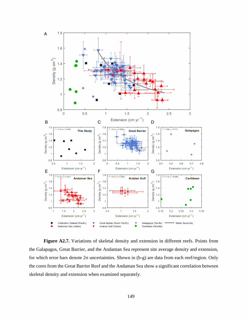
149
Figure A2.7. Variations of skeletal density and extension in different reefs. Points from
the Galapagos, Great Barrier, and the Andaman Sea represent site average density and extension,
for which error bars denote 2σ uncertainties. Shown in (b-g) are data from each reef/region. Only
the cores from the Great Barrier Reef and the Andaman Sea show a significant correlation between
skeletal density and extension when examined separately.
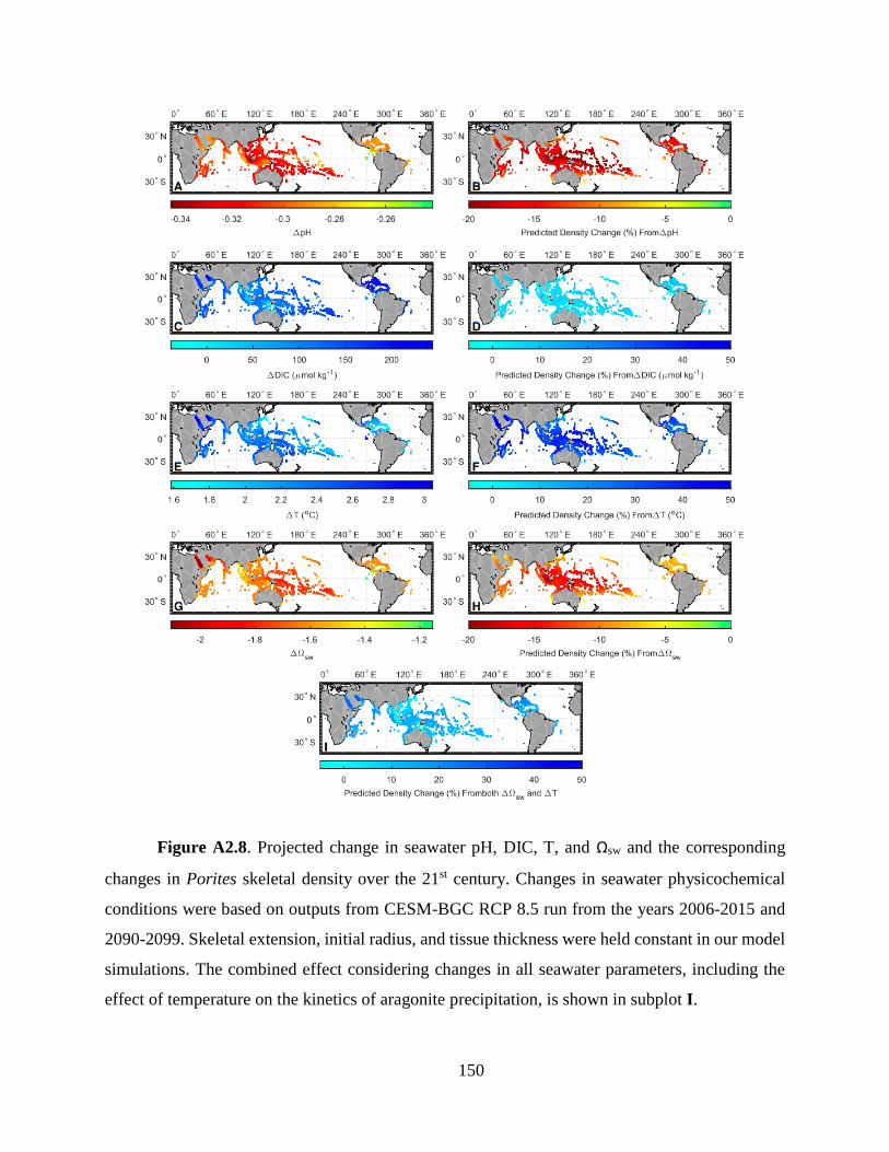
150
Figure A2.8. Projected change in seawater pH, DIC, T, and Ωsw and the corresponding
changes in Porites skeletal density over the 21st century. Changes in seawater physicochemical
conditions were based on outputs from CESM-BGC RCP 8.5 run from the years 2006-2015 and
2090-2099. Skeletal extension, initial radius, and tissue thickness were held constant in our model
simulations. The combined effect considering changes in all seawater parameters, including the
effect of temperature on the kinetics of aragonite precipitation, is shown in subplot I.
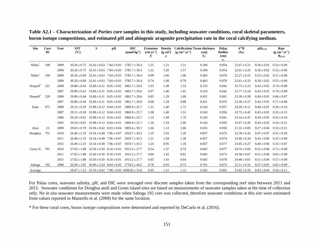
151
Table A2.1 – Characterization of Porites core samples in this study, including seawater conditions, coral skeletal parameters,
boron isotope compositions, and estimated pH and abiogenic aragonite precipitation rate in the coral calcifying medium.
Site Core
ID
Year SST
(oC)
S pH DIC
(μmol kg-1)
Extension
(cm yr-1)
E
Density
(g cm3)
ρ
Calcification
(g cm-2 yr-1)
Tissue thickness
(cm)
Td
Polyp
Radius
(cm)
ro
δ11B
(‰)
pHECM Rate
(g cm-2 yr-1)
RECM
Nikko* 168 2009 30.26 ± 0.75 32.41 ± 0.63 7.84 ± 0.03 1785.7 ± 30.4 1.25 1.21 1.51 0.394 0.054 22.67 ± 0.21 8.36 ± 0.02 0.54 ± 0.09
2008 30.26 ± 0.75 32.41 ± 0.63 7.84 ± 0.03 1785.7 ± 30.4 1.31 1.20 1.57 0.394 0.054 22.61 ± 0.25 8.36 ± 0.02 0.55 ± 0.09
Nikko* 169 2009 30.26 ± 0.69 32.41 ± 0.63 7.84 ± 0.03 1785.7 ± 30.4 0.99 1.06 1.06 0.463 0.078 22.27 ± 0.21 8.33 ± 0.02 0.51 ± 0.08
2008 30.26 ± 0.69 32.41 ± 0.63 7.84 ± 0.03 1785.7 ± 30.4 0.74 1.08 0.79 0.463 0.078 22.61 ± 0.22 8.36 ± 0.02 0.55 ± 0.09
Dropoff* 221 2008 29.80 ± 0.43 33.69 ± 0.31 8.05 ± 0.02 1865.7 ± 29.6 1.03 1.49 1.53 0.333 0.042 23.73 ± 0.23 8.43 ± 0.02 0.74 ± 0.08
2007 29.80 ± 0.43 33.69 ± 0.31 8.05 ± 0.02 1865.7 ± 29.6 0.97 1.46 1.42 0.333 0.042 23.77 ± 0.24 8.43 ± 0.02 0.74 ± 0.08
Dropoff* 229 2008 29.80 ± 0.44 33.69 ± 0.31 8.05 ± 0.02 1865.7 ± 29.6 0.85 1.29 1.09 0.451 0.061 23.30 ± 0.28 8.40 ± 0.02 0.66 ± 0.07
2007 29.80 ± 0.44 33.69 ± 0.31 8.05 ± 0.02 1865.7 ± 29.6 0.68 1.29 0.88 0.451 0.070 23.58 ± 0.27 8.42 ± 0.02 0.71 ± 0.08
Siaes 975 2008 29.21 ± 0.50 33.98 ± 0.12 8.04 ± 0.01 1860.9 ± 25.7 1.23 1.40 1.72 0.543 0.057 24.20 ± 0.11 8.46 ± 0.01 0.36 ± 0.16
2007 29.21 ± 0.50 33.98 ± 0.12 8.04 ± 0.01 1860.9 ± 25.7 1.08 1.40 1.51 0.543 0.056 23.72 ± 0.42 8.43 ± 0.02 0.33 ± 0.15
1996 29.29 ± 0.65 33.98 ± 0.12 8.04 ± 0.01 1860.9 ± 25.7 1.14 1.49 1.70 0.543 0.041 23.14 ± 0.47 8.39 ± 0.03 0.35 ± 0.16
1995 29.29 ± 0.65 33.98 ± 0.12 8.04 ± 0.01 1860.9 ± 25.7 1.34 1.54 2.06 0.543 0.043 23.67 ± 0.26 8.43 ± 0.02 0.54 ± 0.21
Airai 23 2009 29.63 ± 0.70 33.06 ± 0.62 8.03 ± 0.04 1805.6 ± 59.1 1.66 1.12 1.86 0.655 0.050 21.32 ± 0.85 8.27 ± 0.04 0.53 ± 0.21
Donghsa 751 2010 26.40 ± 2.33 33.54 ± 0.49 7.96 ± 0.07 1819.7 ± 45.5 1.25 1.03 1.29 0.857 0.075 23.78 ± 0.43 8.47 ± 0.07 0.51 ± 0.20
2011 26.40 ± 2.33 33.54 ± 0.49 7.96 ± 0.07 1819.7 ± 45.5 1.51 1.04 1.58 0.857 0.074 23.46 ± 0.34 8.45 ± 0.06 0.23 ± 0.08
2012 26.40 ± 2.33 33.54 ± 0.49 7.96 ± 0.07 1819.7 ± 45.5 1.24 0.95 1.18 0.857 0.077 23.65 ± 0.27 8.46 ± 0.06 0.35 ± 0.07
Green Is 701 2010 27.02 ± 1.88 33.50 ± 0.50 8.10 ± 0.01 1913.2 ± 27.7 0.54 1.37 0.74 0.602 0.077 24.74 ± 0.65 8.52 ± 0.06 0.72 ± 0.08
2011 27.02 ± 1.88 33.50 ± 0.50 8.10 ± 0.01 1913.2 ± 27.7 0.60 1.42 0.85 0.602 0.073 24.58 ± 0.67 8.51 ± 0.06 0.65 ± 0.08
2012 27.02 ± 1.88 33.50 ± 0.50 8.10 ± 0.01 1913.2 ± 27.7 0.45 1.43 0.64 0.602 0.078 24.48 ± 0.61 8.51 ± 0.06 0.57 ± 0.09
Saboga 192 2008 26.50 ± 1.02 30.90 ± 2.54 8.04 ± 0.02 1778.5 ± 44.5 0.78 0.93 0.73 0.701 0.073 22.11 ± 0.31 8.37 ± 0.05 0.65 ± 0.09
Average 28.47 ± 1.22 33.10 ± 0.62 7.98 ± 0.03 1838.83 ± 33.6 0.95 1.21 1.12 0.562 0.063 23.42 ± 0.35 8.43 ± 0.04 0.54 ± 0.11
For Palau cores, seawater salinity, pH, and DIC were averaged over discrete samples taken from the corresponding reef sites between 2011 and
2015. Seawater conditions for Donghsa atoll and Green island sites are based on measurements of seawater samples taken at the time of collection
only. No in situ seawater measurements were made when Saboga 192 core was collected, therefore seawater conditions at this site were estimated
from values reported in Manzello et al. (2008) for the same location.
* For these coral cores, boron isotope compositions were determined and reported by DeCarlo et al. (2016).
152
A2.10 References
Allison N, Cohen I, Finch AA, Erez J, Tudhope AW, Facility EIM (2014) Corals concentrate
dissolved inorganic carbon to facilitate calcification. Nat Commun 5:5741
Baker PA, Weber JN (1975) Coral growth rate: Variation with depth. Phys Earth Planet Inter
10:135–139
Barkley HC, Cohen AL, Golbuu Y, Starczak VR, Decarlo TM, Shamberger KEF (2015) Changes
in coral reef communities across a natural gradient in seawater pH. Sci Adv 1–7
Barnes DJ, Lough JM (1993) On the nature and causes of density banding in massive coral
skeletons. J Exp Mar Bio Ecol 167:91–108
Cantin NE, Cohen AL, Karnauskas KB, Tarrant AM, McCorkle DC (2010) Ocean Warming Slows
Coral Growth in the Central Red Sea. 329:322–325
Cohen AL, McConnaughey TA (2003) Geochemical Perspectives on Coral Mineralization. Rev
Mineral Geochemistry 54:151–187
Coles SL, Jokiel PL (1977) Effects of temperature on photosynthesis and respiration in hermatypic
corals. Mar Biol 43:209–216
Comeau S, Cornwall CE, McCulloch MT (2017) Decoupling between the response of coral
calcifying fluid pH and calcification to ocean acidification. Sci Rep 7:7573
Cooper TF, De’ath G, Fabricius KE, Lough JM (2008) Declining coral calcification in massive
Porites in two nearshore regions of the northern Great Barrier Reef. Glob Chang Biol 14:529–
538
Crook ED, Cohen AL, Rebolledo-Vieyra M, Hernandez L, Paytan A (2013) Reduced calcification
and lack of acclimatization by coral colonies growing in areas of persistent natural
acidification. Proc Natl Acad Sci U S A 110:11044–9
Cuif JP, Dauphin Y (2005) The Environment Recording Unit in coral skeletons – a synthesis of
structural and chemical evidences for a biochemically driven, stepping-growth process in
bres. Biogeosciences 2:61–73
153
De’ath G, Lough JM, Fabricius KE (2009) Declining coral calcification on the Great Barrier Reef.
Science (80- ) 323:116–119
Elman JL (1991) On the inclusion of trace materials into massive coral skeletons. Mach Learn
7:195–225
Fabricius KE, Langdon C, Uthicke S, Humphrey C, Noonan S, De ’ath G, Okazaki R, Muehllehner
N, Glas MS, Lough JM (2011) Losers and winners in coral reefs acclimatized to elevated
carbon dioxide concentrations. Nat Clim Chang 1:165–169
Furla P (2000) Furla P , Galgani I , Durand I , Allemand D .. Sources and mechanisms of inorganic
carbon transport for coral calcification and photosynthesis . J Exp. J Exp Biol 3445–3457
Gagan MK, Dunbar GB, Suzuki A (2012) The effect of skeletal mass accumulation in Porites on
coral Sr/Ca and ??18O paleothermometry. Paleoceanography 27:1–16
Hetzinger S, Pfeiff M, Dullo W, Zinke J (2016) A change in coral extension rates and stable
isotopes after El Niño- induced coral bleaching and regional stress events. 1–10
Holcomb M, DeCarlo T, Gaetani G, McCulloch M (2016) Factors affecting B/Ca ratios on
synthetic aragonite. 67–76
Hooidonk R Van, Maynard J, Tamelander J, Gove J (2016) Local-scale projections of coral reef
futures and implications of the Paris Agreement. Nat Publ Gr 1–8
Hughes TP (1987) Skeletal density and growth form of corals. 35:259–266
Huston M (1985) Variation in coral growth rates with depth. Coral Reefs 4:19–25
Linsley BK, Messier RG, Dunbar RB (1999) Assessing between-colony oxygen isotope variability
in the coral Porites iobata at Clipperton Atoll. Coral Reefs 18:13–27
Lough JM, Barnes DJ (2000) Environmental controls on growth of the massive coral Porites. J
Exp Mar Bio Ecol 245:225–243
Manzello DP, Enochs IC, Bruckner A, Renaud PG, Kolodziej G, Budd DA, Carlton R, Glynn PW
(2014) Galapagos coral reef persistence after ENSO warming across an acidification gradient.
154
Geophys Res Lett 41:9001–9008
Mcculloch MT, Olivo JPD, Falter J, Holcomb M, Trotter JA (2017) Coral calcification in a
changing World and the interactive dynamics of pH and DIC upregulation. 1–8
McNeil BI, Matear RJ, Barnes DJ (2004) Coral reef calcification and climate change : The effect
of ocean warming. 31:2–5
Nie B, Chen T, Zhu ML, Wang Y, Zhong J, Zhu Y (1997) Relationship between coral growth rate
and sea surface temperature in the northern part of South China Sea during the past 100 a. Sci
China Ser D Earth Sci 40:173–182
Northdruft LD, Webb GE (2007) Microstructure of common reef-building coral genera Acropora,
Pocillopora, Goniastrea and Porites: constraints on spatial resolution in geochemical
sampling. Facies - Carbonate Sedimentol Paleoecol 53:1–26
Poulsen A, Burns K, Lough J, Brinkman D, Delean S (2006) Trace analysis of hydrocarbons in
coral cores from Saudi Arabia. Org Geochem 37:1913–1930
Shirai K, Sowa K, Watanabe T, Sano Y, Nakamura T, Clode P (2012) Visualization of sub-daily
skeletal growth patterns in massive Porites corals grown in Sr-enriched seawater. J Struct
Biol 180:47–56
Szmant AM (1986) Coral Reefs Reproductive ecology of Caribbean reef corals. 43–53
Tambutté E, Venn AA, Holcomb M, Segonds N, Techer N, Zoccola D, Allemand D, Tambutté S
(2015) Morphological plasticity of the coral skeleton under CO2-driven seawater
acidification. Nat Commun 6:7368
Tanzil JTI, Brown BE, Dunne RP, Lee JN, Kaandorp JA, Todd PA (2013) Regional decline in
growth rates of massive Porites corals in Southeast Asia. Glob Chang Biol 19:3011–3023
Tanzil JTI, Brown BE, Tudhope AW, Dunne RP (2009) Decline in skeletal growth of the coral
Porites lutea from the Andaman Sea, South Thailand between 1984 and 2005. Coral Reefs
28:519–528
Taylor RB, Barnes DJ, Lough JM (1993) Simple-Models of Density Band Formation in Massive
155
Corals. J Exp Mar Bio Ecol 167:109–125
Veron JE., Stafford-Smith M (2000) Corals of the world. Vol 1-3. Australian Institute of Marine
Science, Townsville MC, Qld, Australia
Warner ME, Fitt WK, Schmidt GW (1996) The effects of elevated temperature on the
photosynthetic efficiency of zooxanthellae in hospite from four different species of reef coral:
a novel approach. Plant Cell Environ 19:291–299
Wellington GM, Dunbar RB, Merlen G (1996) Calibration of stable oxygen isotope signatures in
Galpagos corals. Paleoceanography 11:467–480
Wells JW (1956) Scleractinia. Treatise on invertebrate paleontology F. Coelenterata. Geological
Society of America & University of Kansas Press, pp 328–440

156
157
Appendix A3 – Supplementary text, figures,
and data for chapter 3
A3.1 Formulation of the Mantel-Haenszel estimator
An odds ratio can be used to estimate the chance of an outcome occurring (in this case the
formation of a stress band) relative to another, independently observed outcome (in this case coral
bleaching). Here we use it to estimate a given coral community’s propensity to form stress bands
at different levels of bleaching, and to compare the prevalence of stress banding on different reefs.
In this context, the common odds ratio can be expressed as:
𝜓 =𝑝𝑏𝑖/(1 − 𝑝𝑏𝑖)
𝑝𝑠𝑏/(1 − 𝑝𝑠𝑏)
Where 𝑝𝑏𝑖 is the probability of a coral bleaching at a given time, and 𝑝𝑠𝑏 the probability
that a coral has a stress band associated with the same time. If sampled colonies are assumed to
follow a binomial distribution in both the probability to bleach and to form a stress band formation,
the Mantel-Haenszel estimator of the common odds ratio can be expressed as follows:
= ∑ 𝑋𝑗(𝑛𝑗 − 𝑌𝑗)/𝑁𝑗
𝐽𝑗=1
∑ 𝑌𝑗(𝑚𝑗 − 𝑋𝑗)/𝑁𝑗𝐽𝑗=1
Where 𝑋𝑗 is the number out of 𝑚𝑗 corals that produce stress bands, and 𝑌𝑗 is the number
out of 𝑛𝑗 corals that bleach for an event j. Because bleaching data is commonly reported in percent
cover bleached, and not the number of colonies bleached, we estimated 𝑌𝑗 as the number of square
meters bleached (𝑌𝑗∗) out of a total of 𝑛𝑗
∗ square meters. Substituting these values into the equation
above, and treating each bleaching event on each reef as an individual event j, we estimated a
common odds ratio of = 1.11, which implies a near 1 to 1 association between the amount of
stress bands observed in the coral colonies, and the amount of coral cover bleached. The variance
in this relationship was estimated using Equation 2 in the main text, and converted to 2σ = 0.10,
158
implying a very consistent odds ratio between stress band prevalence and observed community
bleaching among reefs, and between events at a single reef (where more than one were observed).
A3.2 Calibration of the percentile based bleaching threshold
We calibrated the ENSO-Neutral Percentile based model of thermal stress to select a
percentile of the climatological SST that maximizes bleaching prediction. We compared bleaching
predictions made using a range of threshold percentiles (84.0th to 99.9th) to the database of
bleaching observations recently published by Donner et al., (2017). In this analysis, we considered
each year at each site an individual event for a total of 𝑛 = 21,384 predictions. In keeping with
the traditional NOAA methodology, bleaching was predicted for an event if the DHW exceeded 4
°C·weeks during a given year at each site. The overall quality of prediction was assessed using the
Gilbert or Equitable Threat Score (ETS) (Fig. A3.1):
𝐸𝑇𝑆 =𝑆 − 𝑆𝑟
𝑆 + 𝐹1 + 𝐹2 − 𝑆𝑟
Where 𝑆 is total number of correct predictions (i.e. bleaching occurred and was predicted
or did not occur and was not predicted) and 𝐹1 and 𝐹2 are type 1 and type 2 errors. 𝑆𝑟 are successes
that can be attributed to random chance, and are defined as:
𝑆𝑟 = (𝑆 + 𝐹1)(𝑆 + 𝐹2)/𝑛
Possible ETS range from -⅓ to 1, with 1 indicating perfect predictive power. Using this
metric, the maximum predictive power of the percentile-based model was found to be at a threshold
percentile of 94.4. We then compared the calibrated ENSO-Neutral Percentile based model to the
traditional MMM model to evaluate the quality of our predictions versus those made using the
established method. When comparing the predictive power of two models using scarce data, such
as bleaching observations, it is critical to assess both type I (false positive) and type II (false
negative) errors as well as the accuracy of predictions as a whole. While some amount of type I
errors is expected (bleaching may likely have occurred but not been documented), an abundance
of type II errors suggests the number of correct predictions a model makes may be a result of over-
159
prediction. As can be seen in Table A3.1, the ENSO-Neutral percentile based DHW have a higher
ETS, and more often correctly predict the bleaching state.
While the ideal validation for this new model would be to compare predictive power in the
Central Pacific relative to higher latitudes, the paucity of observations of bleaching on these
equatorial reefs precludes such an analysis. The methodology of the ENSO-Neutral Percentile
based method is more directly designed to compare thermal stress in equatorial environments with
higher latitudes than the MMM model. Combined with the evidence of equivalent if not superior
prediction at locations where bleaching observations have been made suggest that this model is
better suited to be used in comparing thermal tolerances of equatorial versus higher latitude corals.
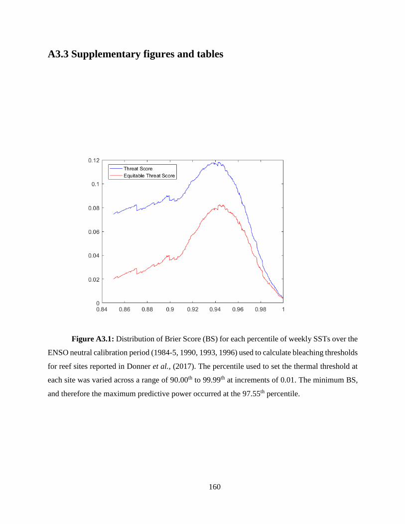
160
A3.3 Supplementary figures and tables
Figure A3.1: Distribution of Brier Score (BS) for each percentile of weekly SSTs over the
ENSO neutral calibration period (1984-5, 1990, 1993, 1996) used to calculate bleaching thresholds
for reef sites reported in Donner et al., (2017). The percentile used to set the thermal threshold at
each site was varied across a range of 90.00th to 99.99th at increments of 0.01. The minimum BS,
and therefore the maximum predictive power occurred at the 97.55th percentile.
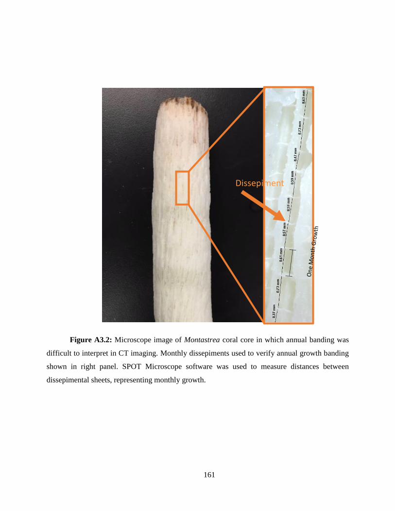
161
Figure A3.2: Microscope image of Montastrea coral core in which annual banding was
difficult to interpret in CT imaging. Monthly dissepiments used to verify annual growth banding
shown in right panel. SPOT Microscope software was used to measure distances between
dissepimental sheets, representing monthly growth.
Dissepiment
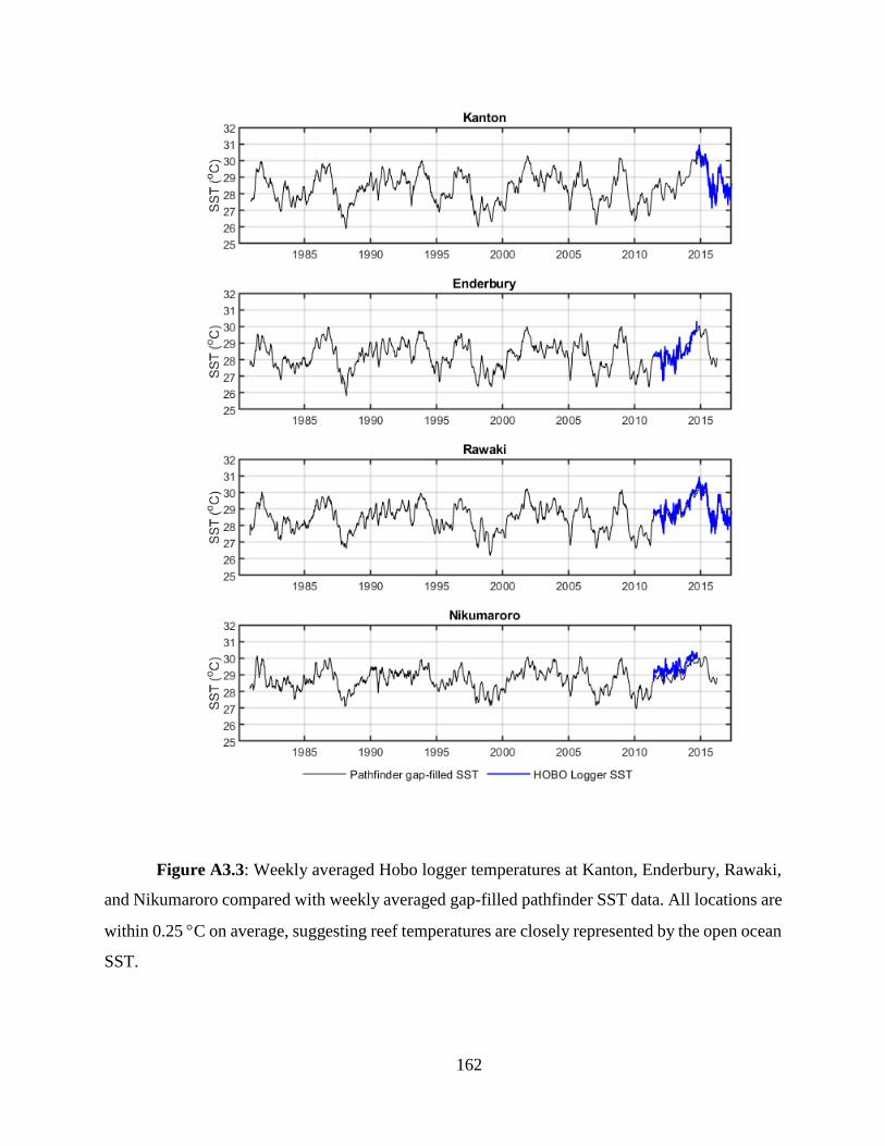
162
Figure A3.3: Weekly averaged Hobo logger temperatures at Kanton, Enderbury, Rawaki,
and Nikumaroro compared with weekly averaged gap-filled pathfinder SST data. All locations are
within 0.25 C on average, suggesting reef temperatures are closely represented by the open ocean
SST.
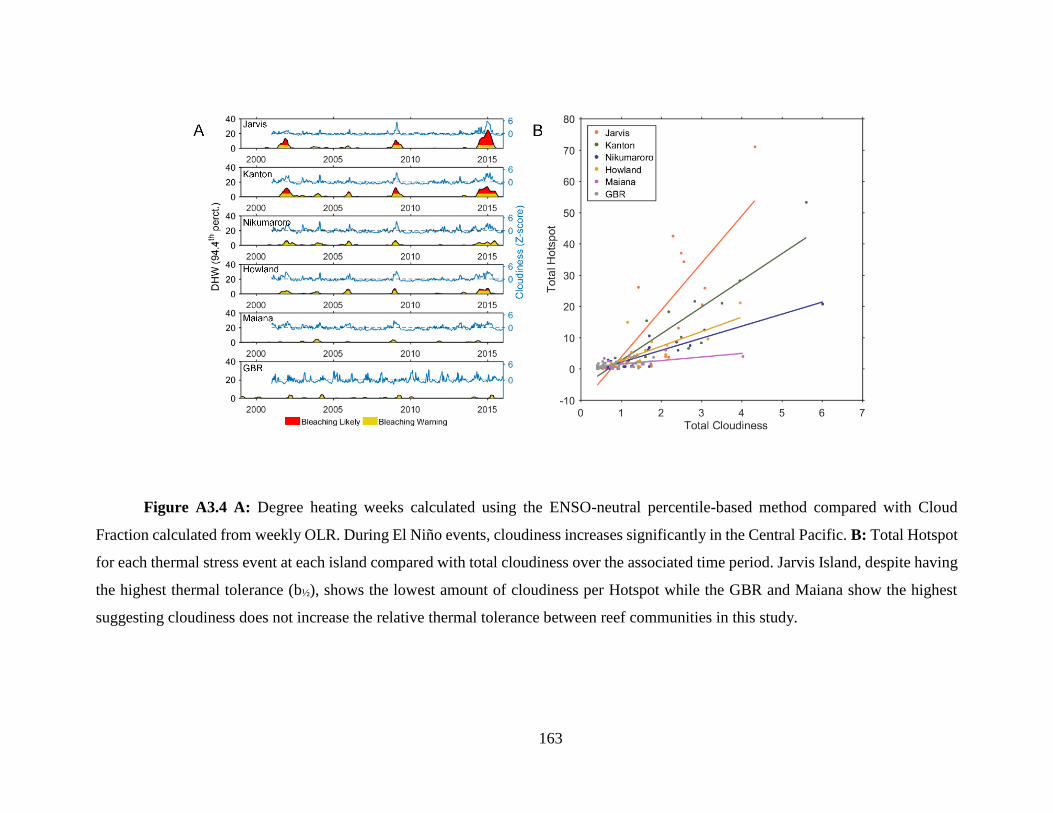
163
Figure A3.4 A: Degree heating weeks calculated using the ENSO-neutral percentile-based method compared with Cloud
Fraction calculated from weekly OLR. During El Niño events, cloudiness increases significantly in the Central Pacific. B: Total Hotspot
for each thermal stress event at each island compared with total cloudiness over the associated time period. Jarvis Island, despite having
the highest thermal tolerance (b½), shows the lowest amount of cloudiness per Hotspot while the GBR and Maiana show the highest
suggesting cloudiness does not increase the relative thermal tolerance between reef communities in this study.
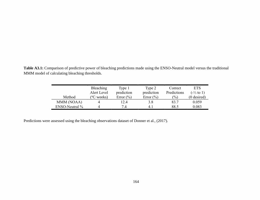
164
Table A3.1: Comparison of predictive power of bleaching predictions made using the ENSO-Neutral model versus the traditional
MMM model of calculating bleaching thresholds.
Predictions were assessed using the bleaching observations dataset of Donner et al., (2017).
Method
Bleaching
Alert Level
(oC·weeks)
Type 1
prediction
Error (%)
Type 2
prediction
Error (%)
Correct
Predictions
(%)
ETS
(-⅓ to 1)
(0 desired)
MMM (NOAA) 4 12.4 3.8 83.7 0.059
ENSO-Neutral % 4 7.4 4.1 88.5 0.083
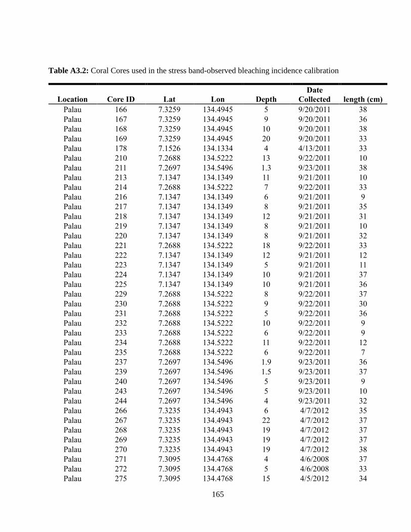
165
Table A3.2: Coral Cores used in the stress band-observed bleaching incidence calibration
Location Core ID Lat Lon Depth Date
Collected length (cm) Palau 166 7.3259 134.4945 5 9/20/2011 38 Palau 167 7.3259 134.4945 9 9/20/2011 36 Palau 168 7.3259 134.4945 10 9/20/2011 38 Palau 169 7.3259 134.4945 20 9/20/2011 33 Palau 178 7.1526 134.1334 4 4/13/2011 33 Palau 210 7.2688 134.5222 13 9/22/2011 10 Palau 211 7.2697 134.5496 1.3 9/23/2011 38 Palau 213 7.1347 134.1349 11 9/21/2011 10 Palau 214 7.2688 134.5222 7 9/22/2011 33 Palau 216 7.1347 134.1349 6 9/21/2011 9 Palau 217 7.1347 134.1349 8 9/21/2011 35 Palau 218 7.1347 134.1349 12 9/21/2011 31 Palau 219 7.1347 134.1349 8 9/21/2011 10 Palau 220 7.1347 134.1349 8 9/21/2011 32 Palau 221 7.2688 134.5222 18 9/22/2011 33 Palau 222 7.1347 134.1349 12 9/21/2011 12 Palau 223 7.1347 134.1349 5 9/21/2011 11 Palau 224 7.1347 134.1349 10 9/21/2011 37 Palau 225 7.1347 134.1349 10 9/21/2011 36 Palau 229 7.2688 134.5222 8 9/22/2011 37 Palau 230 7.2688 134.5222 9 9/22/2011 30 Palau 231 7.2688 134.5222 5 9/22/2011 36 Palau 232 7.2688 134.5222 10 9/22/2011 9 Palau 233 7.2688 134.5222 6 9/22/2011 9 Palau 234 7.2688 134.5222 11 9/22/2011 12 Palau 235 7.2688 134.5222 6 9/22/2011 7 Palau 237 7.2697 134.5496 1.9 9/23/2011 36 Palau 239 7.2697 134.5496 1.5 9/23/2011 37 Palau 240 7.2697 134.5496 5 9/23/2011 9 Palau 243 7.2697 134.5496 5 9/23/2011 10 Palau 244 7.2697 134.5496 4 9/23/2011 32 Palau 266 7.3235 134.4943 6 4/7/2012 35 Palau 267 7.3235 134.4943 22 4/7/2012 37 Palau 268 7.3235 134.4943 19 4/7/2012 37 Palau 269 7.3235 134.4943 19 4/7/2012 37 Palau 270 7.3235 134.4943 19 4/7/2012 38 Palau 271 7.3095 134.4768 4 4/6/2008 37 Palau 272 7.3095 134.4768 5 4/6/2008 33 Palau 275 7.3095 134.4768 15 4/5/2012 34
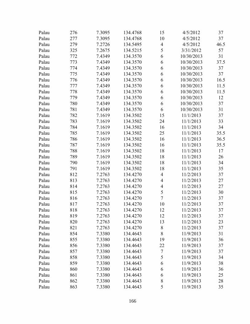
166
Palau 276 7.3095 134.4768 15 4/5/2012 37 Palau 277 7.3095 134.4768 10 4/5/2012 37 Palau 279 7.2726 134.5495 4 4/5/2012 46.5 Palau 325 7.2675 134.5215 5 3/31/2012 57 Palau 772 7.4349 134.3570 6 10/30/2013 31 Palau 773 7.4349 134.3570 6 10/30/2013 37.5 Palau 774 7.4349 134.3570 6 10/30/2013 37 Palau 775 7.4349 134.3570 6 10/30/2013 37 Palau 776 7.4349 134.3570 6 10/30/2013 16.5 Palau 777 7.4349 134.3570 6 10/30/2013 11.5 Palau 778 7.4349 134.3570 6 10/30/2013 11.5 Palau 779 7.4349 134.3570 6 10/30/2013 12 Palau 780 7.4349 134.3570 6 10/30/2013 37 Palau 781 7.4349 134.3570 6 10/30/2013 31 Palau 782 7.1619 134.3502 15 11/1/2013 37 Palau 783 7.1619 134.3502 24 11/1/2013 33 Palau 784 7.1619 134.3502 16 11/1/2013 34 Palau 785 7.1619 134.3502 25 11/1/2013 35.5 Palau 786 7.1619 134.3502 16 11/1/2013 36.5 Palau 787 7.1619 134.3502 16 11/1/2013 35.5 Palau 788 7.1619 134.3502 18 11/1/2013 17 Palau 789 7.1619 134.3502 18 11/1/2013 26 Palau 790 7.1619 134.3502 18 11/1/2013 34 Palau 791 7.1619 134.3502 18 11/1/2013 35 Palau 812 7.2763 134.4270 4 11/2/2013 37 Palau 813 7.2763 134.4270 4 11/2/2013 27 Palau 814 7.2763 134.4270 4 11/2/2013 27 Palau 815 7.2763 134.4270 5 11/2/2013 30 Palau 816 7.2763 134.4270 7 11/2/2013 37 Palau 817 7.2763 134.4270 10 11/2/2013 37 Palau 818 7.2763 134.4270 12 11/2/2013 37 Palau 819 7.2763 134.4270 12 11/2/2013 37 Palau 820 7.2763 134.4270 13 11/2/2013 23 Palau 821 7.2763 134.4270 8 11/2/2013 37 Palau 854 7.3380 134.4643 8 11/9/2013 31 Palau 855 7.3380 134.4643 19 11/9/2013 36 Palau 856 7.3380 134.4643 22 11/9/2013 37 Palau 857 7.3380 134.4643 7 11/9/2013 37 Palau 858 7.3380 134.4643 5 11/9/2013 34 Palau 859 7.3380 134.4643 6 11/9/2013 38 Palau 860 7.3380 134.4643 6 11/9/2013 36 Palau 861 7.3380 134.4643 6 11/9/2013 25 Palau 862 7.3380 134.4643 8 11/9/2013 28 Palau 863 7.3380 134.4643 5 11/9/2013 35
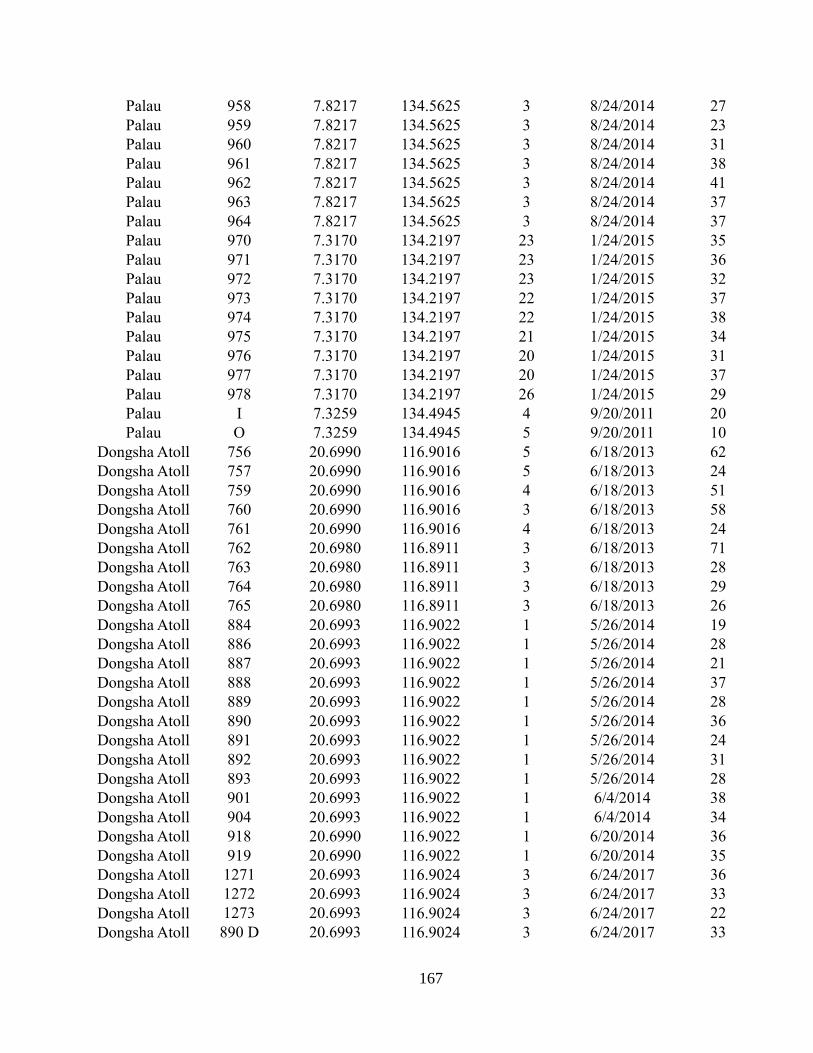
167
Palau 958 7.8217 134.5625 3 8/24/2014 27 Palau 959 7.8217 134.5625 3 8/24/2014 23 Palau 960 7.8217 134.5625 3 8/24/2014 31 Palau 961 7.8217 134.5625 3 8/24/2014 38 Palau 962 7.8217 134.5625 3 8/24/2014 41 Palau 963 7.8217 134.5625 3 8/24/2014 37 Palau 964 7.8217 134.5625 3 8/24/2014 37 Palau 970 7.3170 134.2197 23 1/24/2015 35 Palau 971 7.3170 134.2197 23 1/24/2015 36 Palau 972 7.3170 134.2197 23 1/24/2015 32 Palau 973 7.3170 134.2197 22 1/24/2015 37 Palau 974 7.3170 134.2197 22 1/24/2015 38 Palau 975 7.3170 134.2197 21 1/24/2015 34 Palau 976 7.3170 134.2197 20 1/24/2015 31 Palau 977 7.3170 134.2197 20 1/24/2015 37 Palau 978 7.3170 134.2197 26 1/24/2015 29 Palau I 7.3259 134.4945 4 9/20/2011 20 Palau O 7.3259 134.4945 5 9/20/2011 10
Dongsha Atoll 756 20.6990 116.9016 5 6/18/2013 62 Dongsha Atoll 757 20.6990 116.9016 5 6/18/2013 24 Dongsha Atoll 759 20.6990 116.9016 4 6/18/2013 51 Dongsha Atoll 760 20.6990 116.9016 3 6/18/2013 58 Dongsha Atoll 761 20.6990 116.9016 4 6/18/2013 24 Dongsha Atoll 762 20.6980 116.8911 3 6/18/2013 71 Dongsha Atoll 763 20.6980 116.8911 3 6/18/2013 28 Dongsha Atoll 764 20.6980 116.8911 3 6/18/2013 29 Dongsha Atoll 765 20.6980 116.8911 3 6/18/2013 26 Dongsha Atoll 884 20.6993 116.9022 1 5/26/2014 19 Dongsha Atoll 886 20.6993 116.9022 1 5/26/2014 28 Dongsha Atoll 887 20.6993 116.9022 1 5/26/2014 21 Dongsha Atoll 888 20.6993 116.9022 1 5/26/2014 37 Dongsha Atoll 889 20.6993 116.9022 1 5/26/2014 28 Dongsha Atoll 890 20.6993 116.9022 1 5/26/2014 36 Dongsha Atoll 891 20.6993 116.9022 1 5/26/2014 24 Dongsha Atoll 892 20.6993 116.9022 1 5/26/2014 31 Dongsha Atoll 893 20.6993 116.9022 1 5/26/2014 28 Dongsha Atoll 901 20.6993 116.9022 1 6/4/2014 38 Dongsha Atoll 904 20.6993 116.9022 1 6/4/2014 34 Dongsha Atoll 918 20.6990 116.9022 1 6/20/2014 36 Dongsha Atoll 919 20.6990 116.9022 1 6/20/2014 35 Dongsha Atoll 1271 20.6993 116.9024 3 6/24/2017 36 Dongsha Atoll 1272 20.6993 116.9024 3 6/24/2017 33 Dongsha Atoll 1273 20.6993 116.9024 3 6/24/2017 22 Dongsha Atoll 890 D 20.6993 116.9024 3 6/24/2017 33
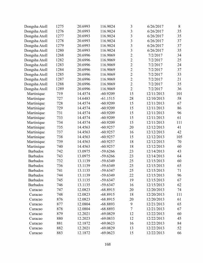
168
Dongsha Atoll 1275 20.6993 116.9024 3 6/26/2017 8 Dongsha Atoll 1276 20.6993 116.9024 3 6/26/2017 35 Dongsha Atoll 1277 20.6993 116.9024 3 6/26/2017 35 Dongsha Atoll 1278 20.6993 116.9024 3 6/26/2017 37 Dongsha Atoll 1279 20.6993 116.9024 3 6/26/2017 37 Dongsha Atoll 1280 20.6993 116.9024 3 6/26/2017 35 Dongsha Atoll 1268 20.6996 116.9069 2 7/2/2017 34 Dongsha Atoll 1282 20.6996 116.9069 2 7/2/2017 25 Dongsha Atoll 1283 20.6996 116.9069 2 7/2/2017 24 Dongsha Atoll 1284 20.6996 116.9069 2 7/2/2017 37 Dongsha Atoll 1285 20.6996 116.9069 2 7/2/2017 33 Dongsha Atoll 1287 20.6996 116.9069 2 7/2/2017 21 Dongsha Atoll 1288 20.6996 116.9069 2 7/2/2017 35 Dongsha Atoll 1289 20.6996 116.9069 2 7/2/2017 36
Martinique 719 14.4574 -60.9209 15 12/11/2013 101 Martinique 727 14.6483 -61.1515 28 12/10/2013 58 Martinique 728 14.4574 -60.9209 15 12/11/2013 67 Martinique 729 14.4574 -60.9209 15 12/11/2013 86 Martinique 731 14.4574 -60.9209 15 12/11/2013 96 Martinique 733 14.4574 -60.9209 15 12/11/2013 61 Martinique 734 14.4574 -60.9209 15 12/11/2013 111 Martinique 735 14.4563 -60.9257 20 12/12/2013 41 Martinique 737 14.4563 -60.9257 16 12/12/2013 42 Martinique 738 14.4563 -60.9257 15 12/12/2013 105 Martinique 739 14.4563 -60.9257 18 12/12/2013 70 Martinique 740 14.4563 -60.9257 18 12/12/2013 60 Barbados 742 13.0975 -59.6266 23 12/14/2013 43 Barbados 743 13.0975 -59.6266 23 12/14/2013 64 Barbados 732 13.1139 -59.6349 25 12/15/2013 60 Barbados 736 13.1139 -59.6349 25 12/15/2013 65 Barbados 741 13.1135 -59.6347 25 12/15/2013 71 Barbados 744 13.1139 -59.6349 22 12/15/2013 96 Barbados 745 13.1135 -59.6347 19 12/15/2013 67 Barbados 746 13.1135 -59.6347 16 12/15/2013 62 Curacao 747 12.0823 -68.8915 20 12/20/2013 74 Curacao 748 12.0823 -68.8915 18 12/20/2013 111 Curacao 876 12.0823 -68.8915 20 12/20/2013 61 Curacao 877 12.0804 -68.8893 9 12/21/2013 65 Curacao 878 12.0804 -68.8893 7 12/21/2013 67 Curacao 879 12.2021 -69.0829 12 12/22/2013 60 Curacao 880 12.2023 -69.0833 12 12/22/2013 45 Curacao 881 12.1872 -69.0623 16 12/22/2013 84 Curacao 882 12.2021 -69.0829 13 12/22/2013 52 Curacao 883 12.1872 -69.0623 15 12/22/2013 66
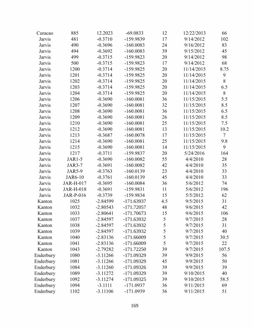
169
Curacao 885 12.2023 -69.0833 12 12/22/2013 66 Jarvis 481 -0.3710 -159.9839 17 9/14/2012 102 Jarvis 490 -0.3696 -160.0083 24 9/16/2012 83 Jarvis 494 -0.3692 -160.0083 39 9/15/2012 45 Jarvis 499 -0.3715 -159.9823 20 9/14/2012 98 Jarvis 500 -0.3715 -159.9823 17 9/14/2012 68 Jarvis 1200 -0.3714 -159.9825 20 11/14/2015 8.75 Jarvis 1201 -0.3714 -159.9825 20 11/14/2015 9 Jarvis 1202 -0.3714 -159.9825 20 11/14/2015 8 Jarvis 1203 -0.3714 -159.9825 20 11/14/2015 6.5 Jarvis 1204 -0.3714 -159.9825 20 11/14/2015 8 Jarvis 1206 -0.3690 -160.0081 36 11/15/2015 5.5 Jarvis 1207 -0.3690 -160.0081 32 11/15/2015 8.5 Jarvis 1208 -0.3690 -160.0081 36 11/15/2015 6.5 Jarvis 1209 -0.3690 -160.0081 26 11/15/2015 8.5 Jarvis 1210 -0.3690 -160.0081 25 11/15/2015 7.5 Jarvis 1212 -0.3690 -160.0081 13 11/15/2015 10.2 Jarvis 1213 -0.3687 -160.0078 17 11/15/2015 7 Jarvis 1214 -0.3690 -160.0081 25 11/15/2015 9.8 Jarvis 1215 -0.3690 -160.0081 14 11/15/2015 9 Jarvis 1217 -0.3711 -159.9837 20 5/24/2016 164 Jarvis JAR1-5 -0.3690 -160.0082 55 4/4/2010 28 Jarvis JAR3-7 -0.3691 -160.0082 42 4/4/2010 35 Jarvis JAR5-9 -0.3763 -160.0139 23 4/4/2010 33 Jarvis JAR6-10 -0.3761 -160.0139 45 4/4/2010 33 Jarvis JAR-H-017 -0.3695 -160.0084 36 5/6/2012 74 Jarvis JAR-H-018 -0.3691 -159.9831 11 5/6/2012 196 Jarvis JAR-P-016 -0.3739 -159.9834 15 5/5/2012 62
Kanton 1025 -2.84599 -171.63937 4.5 9/5/2015 31 Kanton 1032 -2.80543 -171.72057 48 9/6/2015 42 Kanton 1033 -2.80641 -171.70673 15 9/6/2015 106 Kanton 1037 -2.84597 -171.63932 5 9/7/2015 28 Kanton 1038 -2.84597 -171.63932 5 9/7/2015 31 Kanton 1039 -2.84597 -171.63932 5 9/7/2015 40 Kanton 1040 -2.83136 -171.66009 5 9/7/2015 30.5 Kanton 1041 -2.83136 -171.66009 5 9/7/2015 22 Kanton 1043 -2.79282 -171.72250 39 9/7/2015 107.5
Enderbury 1080 -3.11266 -171.09329 39 9/9/2015 56 Enderbury 1081 -3.11266 -171.09329 45 9/9/2015 50 Enderbury 1084 -3.11260 -171.09326 39 9/9/2015 39 Enderbury 1089 -3.11272 -171.09329 39 9/10/2015 40 Enderbury 1092 -3.11274 -171.09325 39 9/10/2015 58.5 Enderbury 1094 -3.1111 -171.0937 36 9/11/2015 69 Enderbury 1102 -3.11106 -171.0939 36 9/11/2015 51
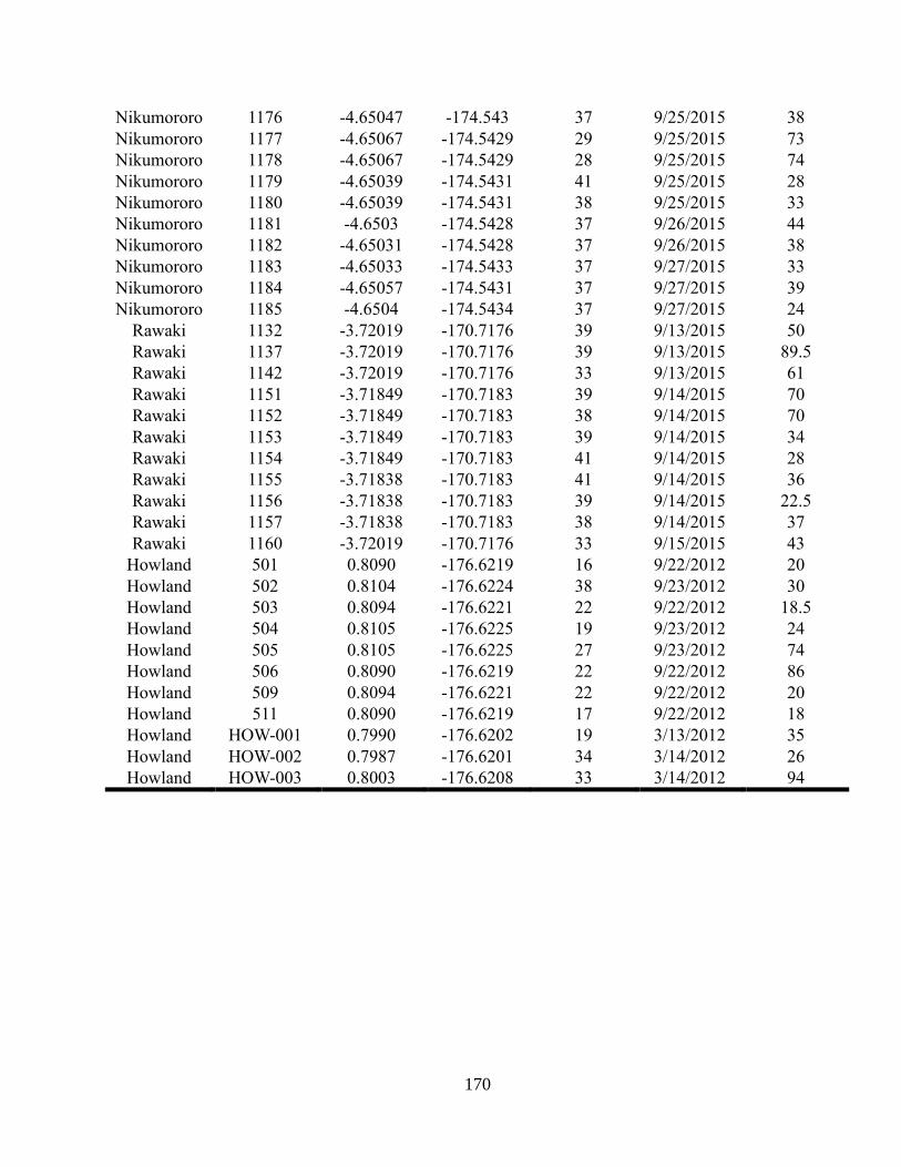
170
Nikumororo 1176 -4.65047 -174.543 37 9/25/2015 38 Nikumororo 1177 -4.65067 -174.5429 29 9/25/2015 73 Nikumororo 1178 -4.65067 -174.5429 28 9/25/2015 74 Nikumororo 1179 -4.65039 -174.5431 41 9/25/2015 28 Nikumororo 1180 -4.65039 -174.5431 38 9/25/2015 33 Nikumororo 1181 -4.6503 -174.5428 37 9/26/2015 44 Nikumororo 1182 -4.65031 -174.5428 37 9/26/2015 38 Nikumororo 1183 -4.65033 -174.5433 37 9/27/2015 33 Nikumororo 1184 -4.65057 -174.5431 37 9/27/2015 39 Nikumororo 1185 -4.6504 -174.5434 37 9/27/2015 24
Rawaki 1132 -3.72019 -170.7176 39 9/13/2015 50 Rawaki 1137 -3.72019 -170.7176 39 9/13/2015 89.5 Rawaki 1142 -3.72019 -170.7176 33 9/13/2015 61 Rawaki 1151 -3.71849 -170.7183 39 9/14/2015 70 Rawaki 1152 -3.71849 -170.7183 38 9/14/2015 70 Rawaki 1153 -3.71849 -170.7183 39 9/14/2015 34 Rawaki 1154 -3.71849 -170.7183 41 9/14/2015 28 Rawaki 1155 -3.71838 -170.7183 41 9/14/2015 36 Rawaki 1156 -3.71838 -170.7183 39 9/14/2015 22.5 Rawaki 1157 -3.71838 -170.7183 38 9/14/2015 37 Rawaki 1160 -3.72019 -170.7176 33 9/15/2015 43
Howland 501 0.8090 -176.6219 16 9/22/2012 20 Howland 502 0.8104 -176.6224 38 9/23/2012 30 Howland 503 0.8094 -176.6221 22 9/22/2012 18.5 Howland 504 0.8105 -176.6225 19 9/23/2012 24 Howland 505 0.8105 -176.6225 27 9/23/2012 74 Howland 506 0.8090 -176.6219 22 9/22/2012 86 Howland 509 0.8094 -176.6221 22 9/22/2012 20 Howland 511 0.8090 -176.6219 17 9/22/2012 18 Howland HOW-001 0.7990 -176.6202 19 3/13/2012 35 Howland HOW-002 0.7987 -176.6201 34 3/14/2012 26 Howland HOW-003 0.8003 -176.6208 33 3/14/2012 94
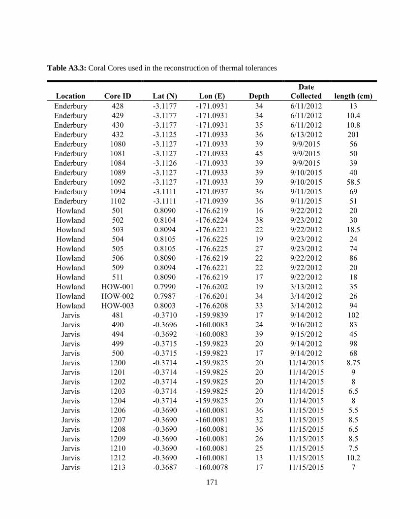
171
Table A3.3: Coral Cores used in the reconstruction of thermal tolerances
Location Core ID Lat (N) Lon (E) Depth Date
Collected length (cm) Enderbury 428 -3.1177 -171.0931 34 6/11/2012 13 Enderbury 429 -3.1177 -171.0931 34 6/11/2012 10.4 Enderbury 430 -3.1177 -171.0931 35 6/11/2012 10.8 Enderbury 432 -3.1125 -171.0933 36 6/13/2012 201 Enderbury 1080 -3.1127 -171.0933 39 9/9/2015 56 Enderbury 1081 -3.1127 -171.0933 45 9/9/2015 50 Enderbury 1084 -3.1126 -171.0933 39 9/9/2015 39 Enderbury 1089 -3.1127 -171.0933 39 9/10/2015 40 Enderbury 1092 -3.1127 -171.0933 39 9/10/2015 58.5 Enderbury 1094 -3.1111 -171.0937 36 9/11/2015 69 Enderbury 1102 -3.1111 -171.0939 36 9/11/2015 51 Howland 501 0.8090 -176.6219 16 9/22/2012 20 Howland 502 0.8104 -176.6224 38 9/23/2012 30 Howland 503 0.8094 -176.6221 22 9/22/2012 18.5 Howland 504 0.8105 -176.6225 19 9/23/2012 24 Howland 505 0.8105 -176.6225 27 9/23/2012 74 Howland 506 0.8090 -176.6219 22 9/22/2012 86 Howland 509 0.8094 -176.6221 22 9/22/2012 20 Howland 511 0.8090 -176.6219 17 9/22/2012 18 Howland HOW-001 0.7990 -176.6202 19 3/13/2012 35 Howland HOW-002 0.7987 -176.6201 34 3/14/2012 26 Howland HOW-003 0.8003 -176.6208 33 3/14/2012 94
Jarvis 481 -0.3710 -159.9839 17 9/14/2012 102 Jarvis 490 -0.3696 -160.0083 24 9/16/2012 83 Jarvis 494 -0.3692 -160.0083 39 9/15/2012 45 Jarvis 499 -0.3715 -159.9823 20 9/14/2012 98 Jarvis 500 -0.3715 -159.9823 17 9/14/2012 68 Jarvis 1200 -0.3714 -159.9825 20 11/14/2015 8.75 Jarvis 1201 -0.3714 -159.9825 20 11/14/2015 9 Jarvis 1202 -0.3714 -159.9825 20 11/14/2015 8 Jarvis 1203 -0.3714 -159.9825 20 11/14/2015 6.5 Jarvis 1204 -0.3714 -159.9825 20 11/14/2015 8 Jarvis 1206 -0.3690 -160.0081 36 11/15/2015 5.5 Jarvis 1207 -0.3690 -160.0081 32 11/15/2015 8.5 Jarvis 1208 -0.3690 -160.0081 36 11/15/2015 6.5 Jarvis 1209 -0.3690 -160.0081 26 11/15/2015 8.5 Jarvis 1210 -0.3690 -160.0081 25 11/15/2015 7.5 Jarvis 1212 -0.3690 -160.0081 13 11/15/2015 10.2 Jarvis 1213 -0.3687 -160.0078 17 11/15/2015 7
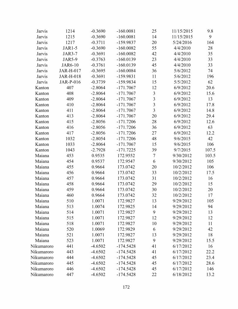
172
Jarvis 1214 -0.3690 -160.0081 25 11/15/2015 9.8 Jarvis 1215 -0.3690 -160.0081 14 11/15/2015 9 Jarvis 1217 -0.3711 -159.9837 20 5/24/2016 164 Jarvis JAR1-5 -0.3690 -160.0082 55 4/4/2010 28 Jarvis JAR3-7 -0.3691 -160.0082 42 4/4/2010 35 Jarvis JAR5-9 -0.3763 -160.0139 23 4/4/2010 33 Jarvis JAR6-10 -0.3761 -160.0139 45 4/4/2010 33 Jarvis JAR-H-017 -0.3695 -160.0084 36 5/6/2012 74 Jarvis JAR-H-018 -0.3691 -159.9831 11 5/6/2012 196 Jarvis JAR-P-016 -0.3739 -159.9834 15 5/5/2012 62
Kanton 407 -2.8064 -171.7067 12 6/9/2012 20.6 Kanton 408 -2.8064 -171.7067 3 6/9/2012 15.6 Kanton 409 -2.8064 -171.7067 3 6/9/2012 13 Kanton 410 -2.8064 -171.7067 3 6/9/2012 17.8 Kanton 411 -2.8064 -171.7067 3 6/9/2012 14.8 Kanton 413 -2.8064 -171.7067 20 6/9/2012 29.4 Kanton 415 -2.8056 -171.7206 28 6/9/2012 12.6 Kanton 416 -2.8056 -171.7206 36 6/9/2012 63 Kanton 417 -2.8056 -171.7206 27 6/9/2012 12.2 Kanton 1032 -2.8054 -171.7206 48 9/6/2015 42 Kanton 1033 -2.8064 -171.7067 15 9/6/2015 106 Kanton 1043 -2.7928 -171.7225 39 9/7/2015 107.5 Maiana 453 0.9535 172.9552 7 9/30/2012 103.5 Maiana 454 0.9537 172.9547 6 9/30/2012 105 Maiana 455 0.9664 173.0742 20 10/2/2012 106 Maiana 456 0.9664 173.0742 33 10/2/2012 17.5 Maiana 457 0.9664 173.0742 31 10/2/2012 16 Maiana 458 0.9664 173.0742 29 10/2/2012 15 Maiana 459 0.9664 173.0742 30 10/2/2012 20 Maiana 460 0.9664 173.0742 32 10/2/2012 17 Maiana 510 1.0071 172.9827 13 9/29/2012 105 Maiana 513 1.0074 172.9825 14 9/29/2012 94 Maiana 514 1.0071 172.9827 9 9/29/2012 13 Maiana 515 1.0071 172.9827 12 9/29/2012 12 Maiana 518 1.0071 172.9827 10 9/29/2012 11 Maiana 520 1.0069 172.9829 6 9/29/2012 42 Maiana 521 1.0071 172.9827 13 9/29/2012 18 Maiana 523 1.0071 172.9827 9 9/29/2012 15.5
Nikumaroro 441 -4.6502 -174.5428 41 6/17/2012 16 Nikumaroro 443 -4.6502 -174.5428 41 6/17/2012 22.2 Nikumaroro 444 -4.6502 -174.5428 45 6/17/2012 23.4 Nikumaroro 445 -4.6502 -174.5428 45 6/17/2012 28.6 Nikumaroro 446 -4.6502 -174.5428 45 6/17/2012 146 Nikumaroro 447 -4.6502 -174.5428 22 6/18/2012 13.2
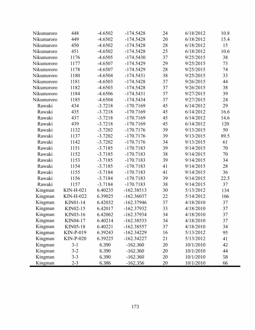
173
Nikumaroro 448 -4.6502 -174.5428 24 6/18/2012 10.8 Nikumaroro 449 -4.6502 -174.5428 20 6/18/2012 15.4 Nikumaroro 450 -4.6502 -174.5428 28 6/18/2012 15 Nikumaroro 451 -4.6502 -174.5428 25 6/18/2012 10.6 Nikumororo 1176 -4.6505 -174.5430 37 9/25/2015 38 Nikumororo 1177 -4.6507 -174.5429 29 9/25/2015 73 Nikumororo 1178 -4.6507 -174.5429 28 9/25/2015 74 Nikumororo 1180 -4.6504 -174.5431 38 9/25/2015 33 Nikumororo 1181 -4.6503 -174.5428 37 9/26/2015 44 Nikumororo 1182 -4.6503 -174.5428 37 9/26/2015 38 Nikumororo 1184 -4.6506 -174.5431 37 9/27/2015 39 Nikumororo 1185 -4.6504 -174.5434 37 9/27/2015 24
Rawaki 434 -3.7218 -170.7169 45 6/14/2012 29 Rawaki 435 -3.7218 -170.7169 45 6/14/2012 16.6 Rawaki 437 -3.7218 -170.7169 45 6/14/2012 14.6 Rawaki 439 -3.7218 -170.7169 45 6/14/2012 120 Rawaki 1132 -3.7202 -170.7176 39 9/13/2015 50 Rawaki 1137 -3.7202 -170.7176 39 9/13/2015 89.5 Rawaki 1142 -3.7202 -170.7176 34 9/13/2015 61 Rawaki 1151 -3.7185 -170.7183 39 9/14/2015 70 Rawaki 1152 -3.7185 -170.7183 38 9/14/2015 70 Rawaki 1153 -3.7185 -170.7183 39 9/14/2015 34 Rawaki 1154 -3.7185 -170.7183 41 9/14/2015 28 Rawaki 1155 -3.7184 -170.7183 41 9/14/2015 36 Rawaki 1156 -3.7184 -170.7183 39 9/14/2015 22.5 Rawaki 1157 -3.7184 -170.7183 38 9/14/2015 37
Kingman KIN-H-021 6.40235 -162.38513 30 5/13/2012 134 Kingman KIN-H-022 6.39025 -162.36037 22 5/14/2012 106 Kingman KIN01-14 6.42032 -162.37946 37 4/18/2010 37 Kingman KIN02-15 6.42017 -162.37932 33 4/18/2010 37 Kingman KIN03-16 6.42062 -162.37934 34 4/18/2010 37 Kingman KIN04-17 6.40214 -162.38533 34 4/18/2010 37 Kingman KIN05-18 6.40221 -162.38557 37 4/18/2010 34 Kingman KIN-P-019 6.39243 -162.34229 16 5/13/2012 95 Kingman KIN-P-020 6.39225 -162.34227 21 5/13/2012 41 Kingman 3-1 6.390 -162.360 20 10/1/2010 42
Kingman 3-2 6.390 -162.360 20 10/1/2010 44
Kingman 3-3 6.390 -162.360 20 10/1/2010 58
Kingman 2-3 6.386 -162.356 20 10/1/2010 66
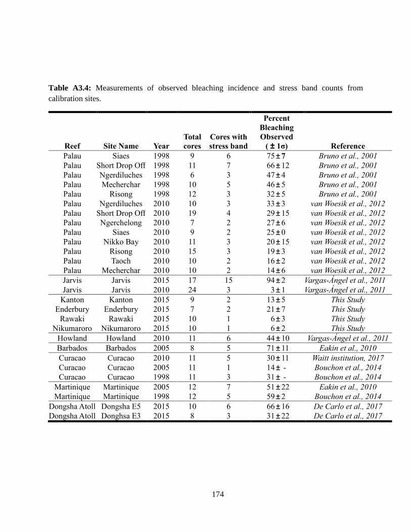
174
Table A3.4: Measurements of observed bleaching incidence and stress band counts from
calibration sites.
Reef Site Name Year Total
cores Cores with
stress band
Percent
Bleaching
Observed ( ± 1σ) Reference
Palau Siaes 1998 9 6 75 ± 7 Bruno et al., 2001 Palau Short Drop Off 1998 11 7 66 ± 12 Bruno et al., 2001 Palau Ngerdiluches 1998 6 3 47 ± 4 Bruno et al., 2001 Palau Mecherchar 1998 10 5 46 ± 5 Bruno et al., 2001 Palau Risong 1998 12 3 32 ± 5 Bruno et al., 2001 Palau Ngerdiluches 2010 10 3 33 ± 3 van Woesik et al., 2012 Palau Short Drop Off 2010 19 4 29 ± 15 van Woesik et al., 2012 Palau Ngerchelong 2010 7 2 27 ± 6 van Woesik et al., 2012 Palau Siaes 2010 9 2 25 ± 0 van Woesik et al., 2012 Palau Nikko Bay 2010 11 3 20 ± 15 van Woesik et al., 2012 Palau Risong 2010 15 3 19 ± 3 van Woesik et al., 2012 Palau Taoch 2010 10 2 16 ± 2 van Woesik et al., 2012 Palau Mecherchar 2010 10 2 14 ± 6 van Woesik et al., 2012 Jarvis Jarvis 2015 17 15 94 ± 2 Vargas-Ángel et al., 2011 Jarvis Jarvis 2010 24 3 3 ± 1 Vargas-Ángel et al., 2011
Kanton Kanton 2015 9 2 13 ± 5 This Study Enderbury Enderbury 2015 7 2 21 ± 7 This Study
Rawaki Rawaki 2015 10 1 6 ± 3 This Study Nikumaroro Nikumaroro 2015 10 1 6 ± 2 This Study
Howland Howland 2010 11 6 44 ± 10 Vargas-Ángel et al., 2011 Barbados Barbados 2005 8 5 71 ± 11 Eakin et al., 2010 Curacao Curacao 2010 11 5 30 ± 11 Waitt institution, 2017 Curacao Curacao 2005 11 1 14 ± - Bouchon et al., 2014 Curacao Curacao 1998 11 3 31 ± - Bouchon et al., 2014
Martinique Martinique 2005 12 7 51 ± 22 Eakin et al., 2010 Martinique Martinique 1998 12 5 59 ± 2 Bouchon et al., 2014
Dongsha Atoll Dongsha E5 2015 10 6 66 ± 16 De Carlo et al., 2017 Dongsha Atoll Donghsa E3 2015 8 3 31 ± 22 De Carlo et al., 2017
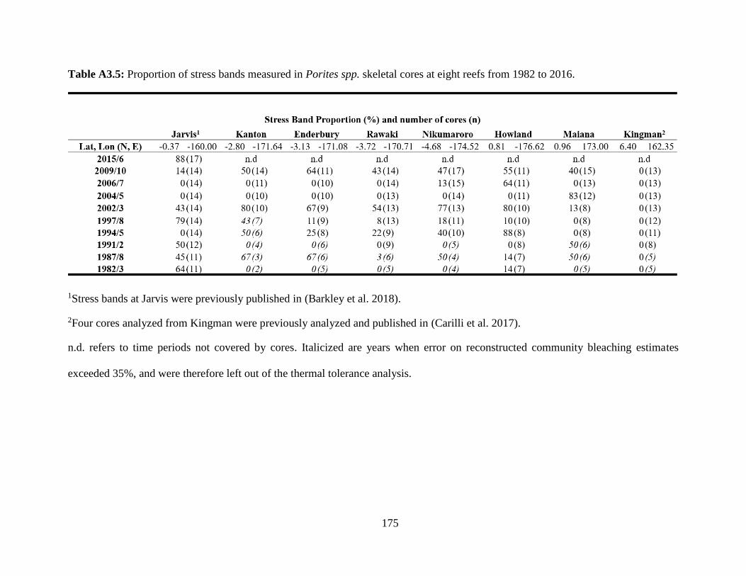
175
Table A3.5: Proportion of stress bands measured in Porites spp. skeletal cores at eight reefs from 1982 to 2016.
1Stress bands at Jarvis were previously published in (Barkley et al. 2018).
2Four cores analyzed from Kingman were previously analyzed and published in (Carilli et al. 2017).
n.d. refers to time periods not covered by cores. Italicized are years when error on reconstructed community bleaching estimates
exceeded 35%, and were therefore left out of the thermal tolerance analysis.
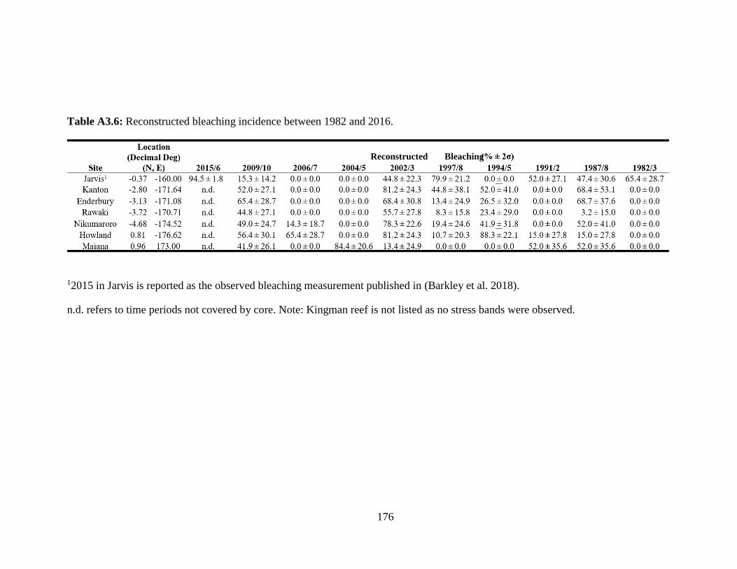
176
Table A3.6: Reconstructed bleaching incidence between 1982 and 2016.
12015 in Jarvis is reported as the observed bleaching measurement published in (Barkley et al. 2018).
n.d. refers to time periods not covered by core. Note: Kingman reef is not listed as no stress bands were observed.
Reconstructed Bleaching
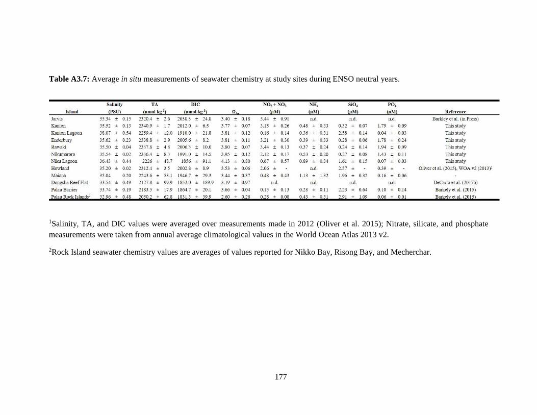
177
Table A3.7: Average in situ measurements of seawater chemistry at study sites during ENSO neutral years.
1Salinity, TA, and DIC values were averaged over measurements made in 2012 (Oliver et al. 2015); Nitrate, silicate, and phosphate
measurements were taken from annual average climatological values in the World Ocean Atlas 2013 v2.
2Rock Island seawater chemistry values are averages of values reported for Nikko Bay, Risong Bay, and Mecherchar.
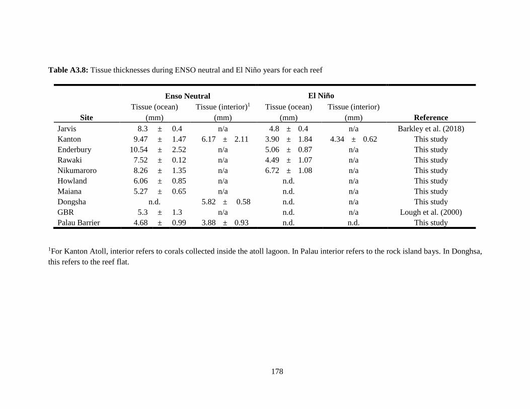
178
Table A3.8: Tissue thicknesses during ENSO neutral and El Niño years for each reef
1For Kanton Atoll, interior refers to corals collected inside the atoll lagoon. In Palau interior refers to the rock island bays. In Donghsa,
this refers to the reef flat.
Site
Enso Neutral El Niño
Reference
Tissue (ocean) Tissue (interior)1 Tissue (ocean) Tissue (interior)
(mm) (mm) (mm) (mm)
Jarvis 8.3 ± 0.4 n/a 4.8 ± 0.4 n/a Barkley et al. (2018)
Kanton 9.47 ± 1.47 6.17 ± 2.11 3.90 ± 1.84 4.34 ± 0.62 This study
Enderbury 10.54 ± 2.52 n/a 5.06 ± 0.87 n/a This study
Rawaki 7.52 ± 0.12 n/a 4.49 ± 1.07 n/a This study
Nikumaroro 8.26 ± 1.35 n/a 6.72 ± 1.08 n/a This study
Howland 6.06 ± 0.85 n/a n.d. n/a This study
Maiana 5.27 ± 0.65 n/a n.d. n/a This study
Dongsha n.d. 5.82 ± 0.58 n.d. n/a This study
GBR 5.3 ± 1.3 n/a n.d. n/a Lough et al. (2000)
Palau Barrier 4.68 ± 0.99 3.88 ± 0.93 n.d. n.d. This study
179
A3.4 References
Barkley HC, Cohen AL, Brainard RE, Mollica NR, Rivera HE, Drenkard EJ, Young CW, Vargas-
Ángel B, Lohmann GP, Decarlo TM, Alpert AE, Lino KC, Oliver TA, Pietro KR, Luu VH
(2018) Repeat bleaching of a central Pacific coral reef over the past six decades (1960-2016).
Nat Biol Commun
Carilli JE, Hartmann AC, Heron SF, Pandolfi JM, Cobb K, Sayani H, Dunbar R, Sandin SA (2017)
Porites coral response to an oceanographic and human impact gradient in the Line Islands.
Limnol Oceanogr 62:2850–2863
Donner SD, Rickbeil GJM, Heron SF (2017) A new, high-resolution global mass coral bleaching
database. PLoS One 12:1–17
Oliver T, Young C, Jeanette C, Pomeroy N (2015) Dissolved inorganic carbon, total alkalinity,
temperature, salinity and other variables collected from profile and discrete sample
observations using CTD, Niskin bottle, and other instruments.

180
181
Appendix A4 – Supplementary text, figures,
and data for chapter 4
A4.1 Laser Data Reduction
When materials are analyzed via LA-ICPMS, it is common to set the associated mass
spectrometer to continuously collect element counts for long periods of time while the laser ablates
aliquots of various samples and standards. This results in data in the format of long time series of
counts of each analyte detected by the mass spectrometer with two dominant features – peaks
during which an analyte is being ablated, and periods of very low counts (noise) between ablations.
The processing and statistical analysis involved in converting this raw data to the form presented
in many studies has unfortunately not been consistent as the field has developed, and no ‘best
practices’ have been established, although there have been some recent efforts (i.e. Branson et al.
2019). Here we draw from these efforts and attempt to lay out our data reduction routine as
explicitly as possible to both elucidate our own methods and also provide a tool to the community
tailored towards coral LA-ICPMS.
A4.1.1 Baseline Subtraction
After importing the raw ICPMS data, we subtract baseline noise from the time series of
each analyte by identifying periods between ablations during the run. This is nominally set to time
periods when the ICPMS detected fewer than 3000 total counts for longer than 10 seconds. These
values may be adjusted to best fit the specific ICPMS setup and sampling interval. We then reduce
these intervals to single points centered within the interval and at the median analyte value over
the interval. We then apply a Piecewise Cubic Hermite Interpolating Polynomial between the noise
points and subtract the corresponding fit from each analyte.
A4.1.2 Peak Identification
Once baseline corrected, peaks are identified via a guess-and-check routine. In short,
standard position and interval are specified, and peaks in the run are then automatically identified
based on a select analyte or the sum total of analytes (total beam). For our analysis we used 43Ca
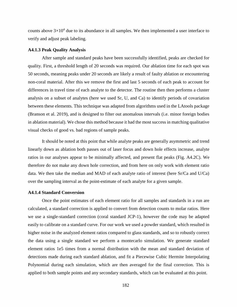
182
counts above 3×10⁴ due to its abundance in all samples. We then implemented a user interface to
verify and adjust peak labeling.
A4.1.3 Peak Quality Analysis
After sample and standard peaks have been successfully identified, peaks are checked for
quality. First, a threshold length of 20 seconds was required. Our ablation time for each spot was
50 seconds, meaning peaks under 20 seconds are likely a result of faulty ablation or encountering
non-coral material. After this we remove the first and last 5 seconds of each peak to account for
differences in travel time of each analyte to the detector. The routine then then performs a cluster
analysis on a subset of analytes (here we used Sr, U, and Ca) to identify periods of covariation
between these elements. This technique was adapted from algorithms used in the LAtools package
(Branson et al. 2019), and is designed to filter out anomalous intervals (i.e. minor foreign bodies
in ablation material). We chose this method because it had the most success in matching qualitative
visual checks of good vs. bad regions of sample peaks.
It should be noted at this point that while analyte peaks are generally asymmetric and trend
linearly down as ablation both passes out of laser focus and down hole effects increase, analyte
ratios in our analyses appear to be minimally affected, and present flat peaks (Fig. A4.2C). We
therefore do not make any down hole correction, and from here on only work with element ratio
data. We then take the median and MAD of each analyte ratio of interest (here Sr/Ca and U/Ca)
over the sampling interval as the point-estimate of each analyte for a given sample.
A4.1.4 Standard Conversion
Once the point estimates of each element ratio for all samples and standards in a run are
calculated, a standard correction is applied to convert from detection counts to molar ratios. Here
we use a single-standard correction (coral standard JCP-1), however the code may be adapted
easily to calibrate on a standard curve. For our work we used a powder standard, which resulted in
higher noise in the analyzed element ratios compared to glass standards, and so to robustly correct
the data using a single standard we perform a montecarlo simulation. We generate standard
element ratios 1e5 times from a normal distribution with the mean and standard deviation of
detections made during each standard ablation, and fit a Piecewise Cubic Hermite Interpolating
Polynomial during each simulation, which are then averaged for the final correction. This is
applied to both sample points and any secondary standards, which can be evaluated at this point.
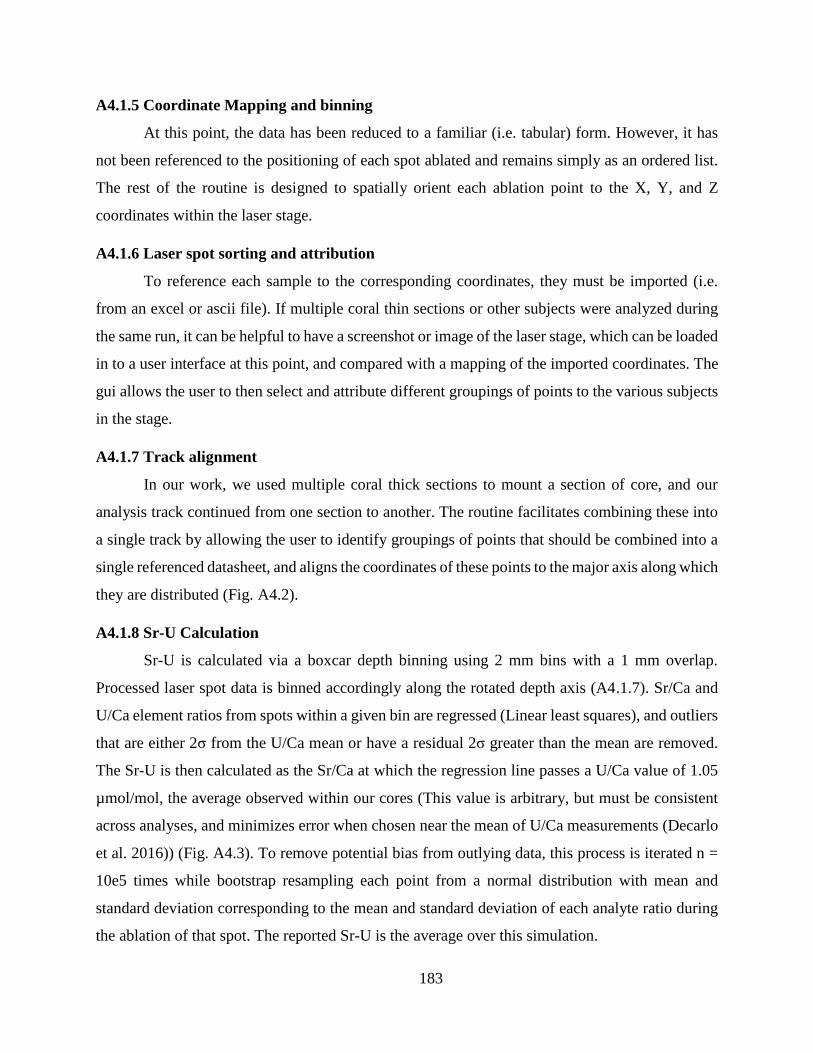
183
A4.1.5 Coordinate Mapping and binning
At this point, the data has been reduced to a familiar (i.e. tabular) form. However, it has
not been referenced to the positioning of each spot ablated and remains simply as an ordered list.
The rest of the routine is designed to spatially orient each ablation point to the X, Y, and Z
coordinates within the laser stage.
A4.1.6 Laser spot sorting and attribution
To reference each sample to the corresponding coordinates, they must be imported (i.e.
from an excel or ascii file). If multiple coral thin sections or other subjects were analyzed during
the same run, it can be helpful to have a screenshot or image of the laser stage, which can be loaded
in to a user interface at this point, and compared with a mapping of the imported coordinates. The
gui allows the user to then select and attribute different groupings of points to the various subjects
in the stage.
A4.1.7 Track alignment
In our work, we used multiple coral thick sections to mount a section of core, and our
analysis track continued from one section to another. The routine facilitates combining these into
a single track by allowing the user to identify groupings of points that should be combined into a
single referenced datasheet, and aligns the coordinates of these points to the major axis along which
they are distributed (Fig. A4.2).
A4.1.8 Sr-U Calculation
Sr-U is calculated via a boxcar depth binning using 2 mm bins with a 1 mm overlap.
Processed laser spot data is binned accordingly along the rotated depth axis (A4.1.7). Sr/Ca and
U/Ca element ratios from spots within a given bin are regressed (Linear least squares), and outliers
that are either 2σ from the U/Ca mean or have a residual 2σ greater than the mean are removed.
The Sr-U is then calculated as the Sr/Ca at which the regression line passes a U/Ca value of 1.05
µmol/mol, the average observed within our cores (This value is arbitrary, but must be consistent
across analyses, and minimizes error when chosen near the mean of U/Ca measurements (Decarlo
et al. 2016)) (Fig. A4.3). To remove potential bias from outlying data, this process is iterated n =
10e5 times while bootstrap resampling each point from a normal distribution with mean and
standard deviation corresponding to the mean and standard deviation of each analyte ratio during
the ablation of that spot. The reported Sr-U is the average over this simulation.
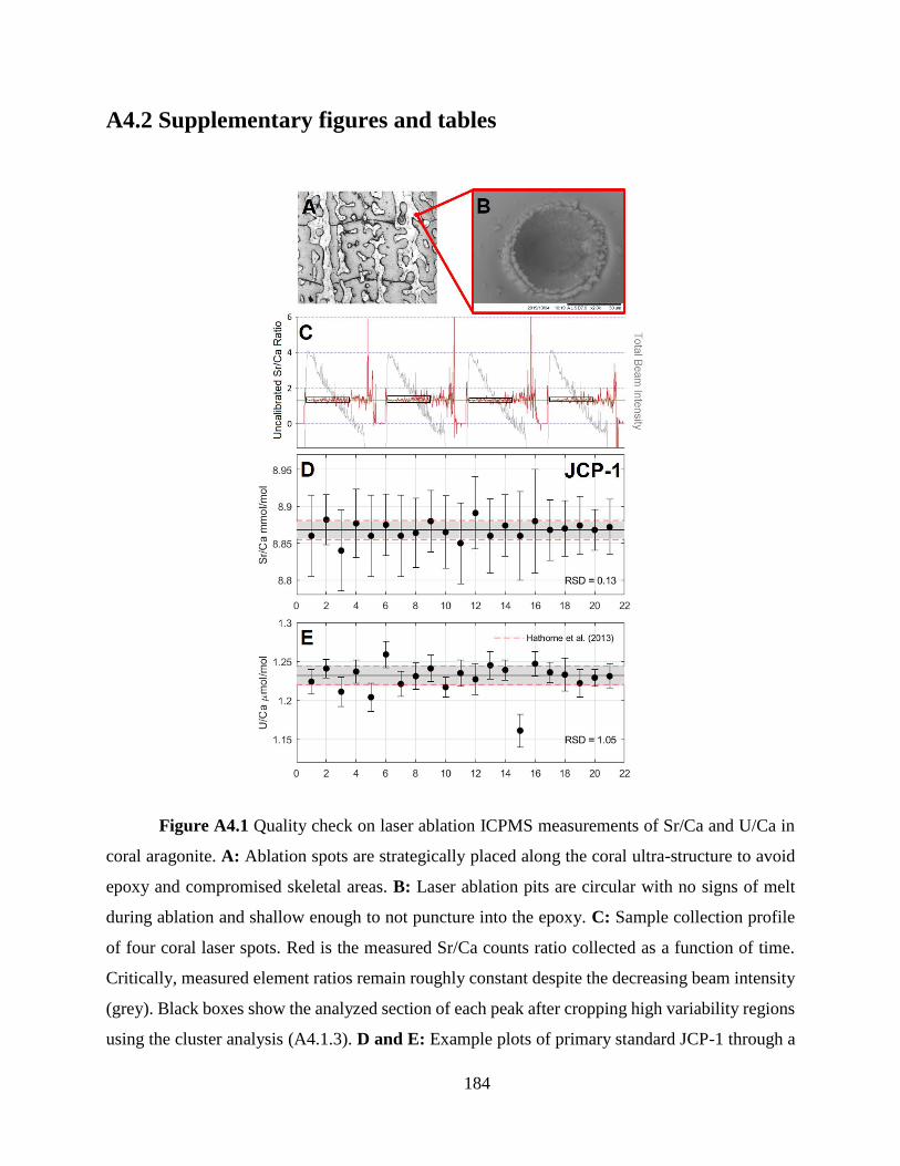
184
A4.2 Supplementary figures and tables
Figure A4.1 Quality check on laser ablation ICPMS measurements of Sr/Ca and U/Ca in
coral aragonite. A: Ablation spots are strategically placed along the coral ultra-structure to avoid
epoxy and compromised skeletal areas. B: Laser ablation pits are circular with no signs of melt
during ablation and shallow enough to not puncture into the epoxy. C: Sample collection profile
of four coral laser spots. Red is the measured Sr/Ca counts ratio collected as a function of time.
Critically, measured element ratios remain roughly constant despite the decreasing beam intensity
(grey). Black boxes show the analyzed section of each peak after cropping high variability regions
using the cluster analysis (A4.1.3). D and E: Example plots of primary standard JCP-1 through a
185
6-hour run. Grey shading = standard deviation about the mean (black line). Dashed red lines in D
and E are the median within-lab standard deviation of an inter-lab comparison study analyzing
Sr/Ca (21 labs) and U/Ca (8 labs) in JCP-1 using solution analyses (Hathorne et al. 2013). Error
bars represent 1. During the run shown, one outlying U/Ca measurement was made which we
attribute to inhomogeneities in the powder standard.
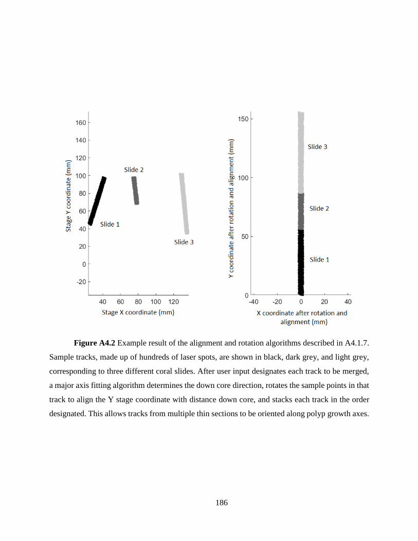
186
Figure A4.2 Example result of the alignment and rotation algorithms described in A4.1.7.
Sample tracks, made up of hundreds of laser spots, are shown in black, dark grey, and light grey,
corresponding to three different coral slides. After user input designates each track to be merged,
a major axis fitting algorithm determines the down core direction, rotates the sample points in that
track to align the Y stage coordinate with distance down core, and stacks each track in the order
designated. This allows tracks from multiple thin sections to be oriented along polyp growth axes.
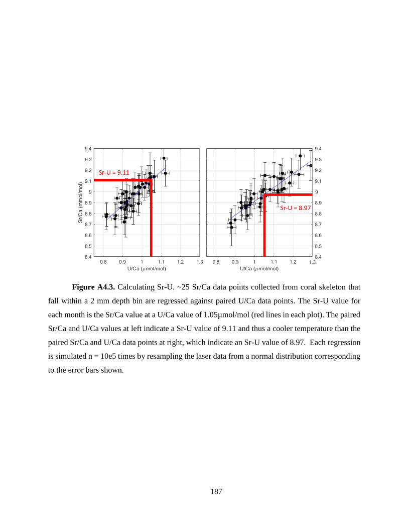
187
Figure A4.3. Calculating Sr-U. ~25 Sr/Ca data points collected from coral skeleton that
fall within a 2 mm depth bin are regressed against paired U/Ca data points. The Sr-U value for
each month is the Sr/Ca value at a U/Ca value of 1.05µmol/mol (red lines in each plot). The paired
Sr/Ca and U/Ca values at left indicate a Sr-U value of 9.11 and thus a cooler temperature than the
paired Sr/Ca and U/Ca data points at right, which indicate an Sr-U value of 8.97. Each regression
is simulated n = 10e5 times by resampling the laser data from a normal distribution corresponding
to the error bars shown.
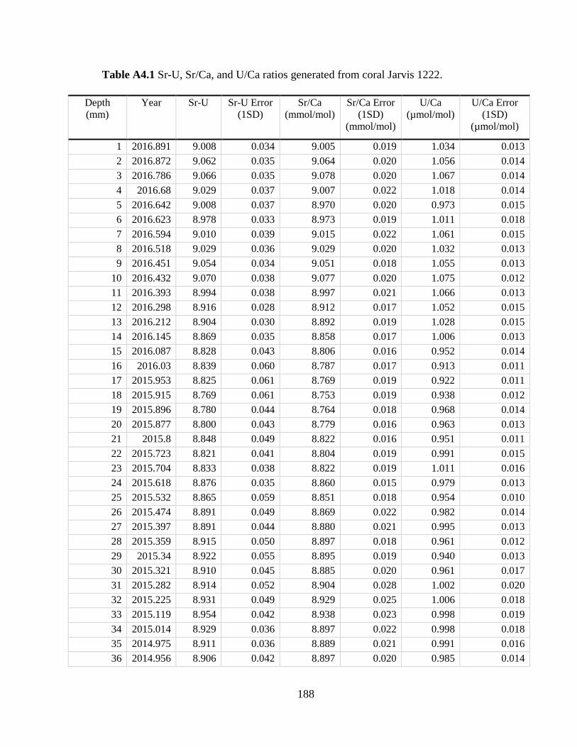
188
Table A4.1 Sr-U, Sr/Ca, and U/Ca ratios generated from coral Jarvis 1222.
Depth
(mm)
Year Sr-U Sr-U Error
(1SD)
Sr/Ca
(mmol/mol)
Sr/Ca Error
(1SD)
(mmol/mol)
U/Ca
(µmol/mol)
U/Ca Error
(1SD)
(µmol/mol)
1 2016.891 9.008 0.034 9.005 0.019 1.034 0.013
2 2016.872 9.062 0.035 9.064 0.020 1.056 0.014
3 2016.786 9.066 0.035 9.078 0.020 1.067 0.014
4 2016.68 9.029 0.037 9.007 0.022 1.018 0.014
5 2016.642 9.008 0.037 8.970 0.020 0.973 0.015
6 2016.623 8.978 0.033 8.973 0.019 1.011 0.018
7 2016.594 9.010 0.039 9.015 0.022 1.061 0.015
8 2016.518 9.029 0.036 9.029 0.020 1.032 0.013
9 2016.451 9.054 0.034 9.051 0.018 1.055 0.013
10 2016.432 9.070 0.038 9.077 0.020 1.075 0.012
11 2016.393 8.994 0.038 8.997 0.021 1.066 0.013
12 2016.298 8.916 0.028 8.912 0.017 1.052 0.015
13 2016.212 8.904 0.030 8.892 0.019 1.028 0.015
14 2016.145 8.869 0.035 8.858 0.017 1.006 0.013
15 2016.087 8.828 0.043 8.806 0.016 0.952 0.014
16 2016.03 8.839 0.060 8.787 0.017 0.913 0.011
17 2015.953 8.825 0.061 8.769 0.019 0.922 0.011
18 2015.915 8.769 0.061 8.753 0.019 0.938 0.012
19 2015.896 8.780 0.044 8.764 0.018 0.968 0.014
20 2015.877 8.800 0.043 8.779 0.016 0.963 0.013
21 2015.8 8.848 0.049 8.822 0.016 0.951 0.011
22 2015.723 8.821 0.041 8.804 0.019 0.991 0.015
23 2015.704 8.833 0.038 8.822 0.019 1.011 0.016
24 2015.618 8.876 0.035 8.860 0.015 0.979 0.013
25 2015.532 8.865 0.059 8.851 0.018 0.954 0.010
26 2015.474 8.891 0.049 8.869 0.022 0.982 0.014
27 2015.397 8.891 0.044 8.880 0.021 0.995 0.013
28 2015.359 8.915 0.050 8.897 0.018 0.961 0.012
29 2015.34 8.922 0.055 8.895 0.019 0.940 0.013
30 2015.321 8.910 0.045 8.885 0.020 0.961 0.017
31 2015.282 8.914 0.052 8.904 0.028 1.002 0.020
32 2015.225 8.931 0.049 8.929 0.025 1.006 0.018
33 2015.119 8.954 0.042 8.938 0.023 0.998 0.019
34 2015.014 8.929 0.036 8.897 0.022 0.998 0.018
35 2014.975 8.911 0.036 8.889 0.021 0.991 0.016
36 2014.956 8.906 0.042 8.897 0.020 0.985 0.014
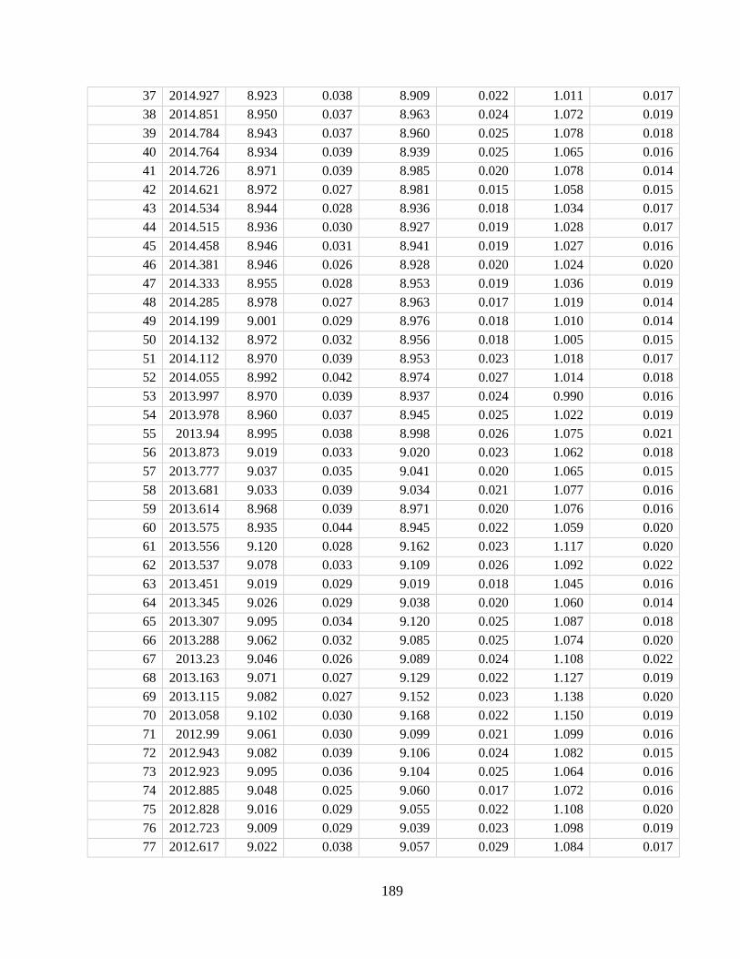
189
37 2014.927 8.923 0.038 8.909 0.022 1.011 0.017
38 2014.851 8.950 0.037 8.963 0.024 1.072 0.019
39 2014.784 8.943 0.037 8.960 0.025 1.078 0.018
40 2014.764 8.934 0.039 8.939 0.025 1.065 0.016
41 2014.726 8.971 0.039 8.985 0.020 1.078 0.014
42 2014.621 8.972 0.027 8.981 0.015 1.058 0.015
43 2014.534 8.944 0.028 8.936 0.018 1.034 0.017
44 2014.515 8.936 0.030 8.927 0.019 1.028 0.017
45 2014.458 8.946 0.031 8.941 0.019 1.027 0.016
46 2014.381 8.946 0.026 8.928 0.020 1.024 0.020
47 2014.333 8.955 0.028 8.953 0.019 1.036 0.019
48 2014.285 8.978 0.027 8.963 0.017 1.019 0.014
49 2014.199 9.001 0.029 8.976 0.018 1.010 0.014
50 2014.132 8.972 0.032 8.956 0.018 1.005 0.015
51 2014.112 8.970 0.039 8.953 0.023 1.018 0.017
52 2014.055 8.992 0.042 8.974 0.027 1.014 0.018
53 2013.997 8.970 0.039 8.937 0.024 0.990 0.016
54 2013.978 8.960 0.037 8.945 0.025 1.022 0.019
55 2013.94 8.995 0.038 8.998 0.026 1.075 0.021
56 2013.873 9.019 0.033 9.020 0.023 1.062 0.018
57 2013.777 9.037 0.035 9.041 0.020 1.065 0.015
58 2013.681 9.033 0.039 9.034 0.021 1.077 0.016
59 2013.614 8.968 0.039 8.971 0.020 1.076 0.016
60 2013.575 8.935 0.044 8.945 0.022 1.059 0.020
61 2013.556 9.120 0.028 9.162 0.023 1.117 0.020
62 2013.537 9.078 0.033 9.109 0.026 1.092 0.022
63 2013.451 9.019 0.029 9.019 0.018 1.045 0.016
64 2013.345 9.026 0.029 9.038 0.020 1.060 0.014
65 2013.307 9.095 0.034 9.120 0.025 1.087 0.018
66 2013.288 9.062 0.032 9.085 0.025 1.074 0.020
67 2013.23 9.046 0.026 9.089 0.024 1.108 0.022
68 2013.163 9.071 0.027 9.129 0.022 1.127 0.019
69 2013.115 9.082 0.027 9.152 0.023 1.138 0.020
70 2013.058 9.102 0.030 9.168 0.022 1.150 0.019
71 2012.99 9.061 0.030 9.099 0.021 1.099 0.016
72 2012.943 9.082 0.039 9.106 0.024 1.082 0.015
73 2012.923 9.095 0.036 9.104 0.025 1.064 0.016
74 2012.885 9.048 0.025 9.060 0.017 1.072 0.016
75 2012.828 9.016 0.029 9.055 0.022 1.108 0.020
76 2012.723 9.009 0.029 9.039 0.023 1.098 0.019
77 2012.617 9.022 0.038 9.057 0.029 1.084 0.017
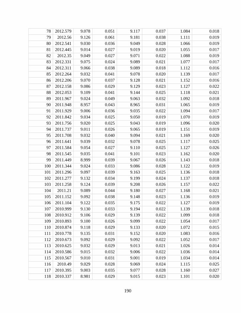
190
78 2012.579 9.078 0.051 9.117 0.037 1.084 0.018
79 2012.56 9.126 0.061 9.181 0.038 1.111 0.019
80 2012.541 9.030 0.036 9.049 0.028 1.066 0.019
81 2012.445 9.014 0.027 9.019 0.020 1.055 0.017
82 2012.35 9.049 0.027 9.071 0.022 1.088 0.019
83 2012.331 9.075 0.024 9.089 0.021 1.077 0.017
84 2012.311 9.066 0.038 9.089 0.018 1.112 0.016
85 2012.264 9.032 0.041 9.078 0.020 1.139 0.017
86 2012.206 9.070 0.037 9.128 0.021 1.152 0.016
87 2012.158 9.086 0.029 9.129 0.023 1.127 0.022
88 2012.053 9.109 0.041 9.144 0.025 1.118 0.021
89 2011.967 9.024 0.049 9.063 0.032 1.092 0.018
90 2011.948 8.957 0.043 8.965 0.031 1.065 0.019
91 2011.929 9.006 0.036 9.035 0.022 1.094 0.017
92 2011.842 9.034 0.025 9.050 0.019 1.070 0.019
93 2011.756 9.020 0.025 9.043 0.019 1.096 0.020
94 2011.737 9.011 0.026 9.065 0.019 1.151 0.019
95 2011.708 9.032 0.040 9.094 0.021 1.169 0.020
96 2011.641 9.039 0.032 9.078 0.025 1.117 0.025
97 2011.584 9.054 0.027 9.110 0.025 1.127 0.026
98 2011.545 9.035 0.041 9.101 0.023 1.162 0.020
99 2011.449 8.999 0.039 9.067 0.026 1.143 0.018
100 2011.344 9.024 0.033 9.086 0.028 1.122 0.019
101 2011.296 9.097 0.039 9.163 0.025 1.136 0.018
102 2011.277 9.132 0.034 9.199 0.024 1.137 0.018
103 2011.258 9.124 0.039 9.208 0.026 1.157 0.022
104 2011.21 9.089 0.044 9.180 0.027 1.168 0.021
105 2011.152 9.092 0.038 9.148 0.023 1.136 0.019
106 2011.104 9.122 0.035 9.175 0.022 1.127 0.019
107 2010.999 9.130 0.033 9.194 0.022 1.139 0.018
108 2010.912 9.106 0.029 9.139 0.022 1.099 0.018
109 2010.893 9.100 0.026 9.099 0.022 1.054 0.017
110 2010.874 9.118 0.029 9.133 0.020 1.072 0.015
111 2010.778 9.135 0.031 9.152 0.020 1.083 0.016
112 2010.673 9.092 0.029 9.092 0.022 1.052 0.017
113 2010.625 9.032 0.029 9.013 0.021 1.026 0.014
114 2010.586 9.015 0.032 9.006 0.022 1.036 0.014
115 2010.567 9.010 0.031 9.001 0.019 1.034 0.014
116 2010.49 9.029 0.028 9.069 0.024 1.115 0.025
117 2010.395 9.003 0.035 9.077 0.028 1.160 0.027
118 2010.337 8.981 0.029 9.015 0.023 1.101 0.020
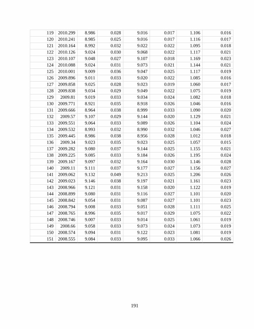
191
119 2010.299 8.986 0.028 9.016 0.017 1.106 0.016
120 2010.241 8.985 0.025 9.016 0.017 1.116 0.017
121 2010.164 8.992 0.032 9.022 0.022 1.095 0.018
122 2010.126 9.024 0.030 9.068 0.022 1.117 0.021
123 2010.107 9.048 0.027 9.107 0.018 1.169 0.023
124 2010.088 9.024 0.031 9.073 0.021 1.144 0.021
125 2010.001 9.009 0.036 9.047 0.025 1.117 0.019
126 2009.896 9.011 0.033 9.020 0.022 1.085 0.016
127 2009.858 9.025 0.028 9.023 0.019 1.060 0.017
128 2009.838 9.034 0.029 9.049 0.022 1.075 0.019
129 2009.81 9.019 0.033 9.034 0.024 1.082 0.018
130 2009.771 8.921 0.035 8.918 0.026 1.046 0.016
131 2009.666 8.964 0.038 8.999 0.033 1.090 0.020
132 2009.57 9.107 0.029 9.144 0.020 1.129 0.021
133 2009.551 9.064 0.033 9.089 0.026 1.104 0.024
134 2009.532 8.993 0.032 8.990 0.032 1.046 0.027
135 2009.445 8.986 0.038 8.956 0.028 1.012 0.018
136 2009.34 9.023 0.035 9.023 0.025 1.057 0.015
137 2009.282 9.080 0.037 9.144 0.025 1.155 0.021
138 2009.225 9.085 0.033 9.184 0.026 1.195 0.024
139 2009.167 9.097 0.032 9.164 0.030 1.146 0.028
140 2009.11 9.111 0.037 9.177 0.027 1.156 0.027
141 2009.062 9.132 0.049 9.213 0.025 1.206 0.026
142 2009.023 9.146 0.038 9.197 0.021 1.161 0.023
143 2008.966 9.121 0.031 9.158 0.020 1.122 0.019
144 2008.899 9.080 0.031 9.116 0.027 1.101 0.020
145 2008.842 9.054 0.031 9.087 0.027 1.101 0.023
146 2008.794 9.008 0.033 9.051 0.028 1.111 0.025
147 2008.765 8.996 0.035 9.017 0.029 1.075 0.022
148 2008.746 9.007 0.033 9.014 0.025 1.061 0.019
149 2008.66 9.058 0.033 9.073 0.024 1.073 0.019
150 2008.574 9.094 0.031 9.122 0.023 1.081 0.019
151 2008.555 9.084 0.033 9.095 0.033 1.066 0.026
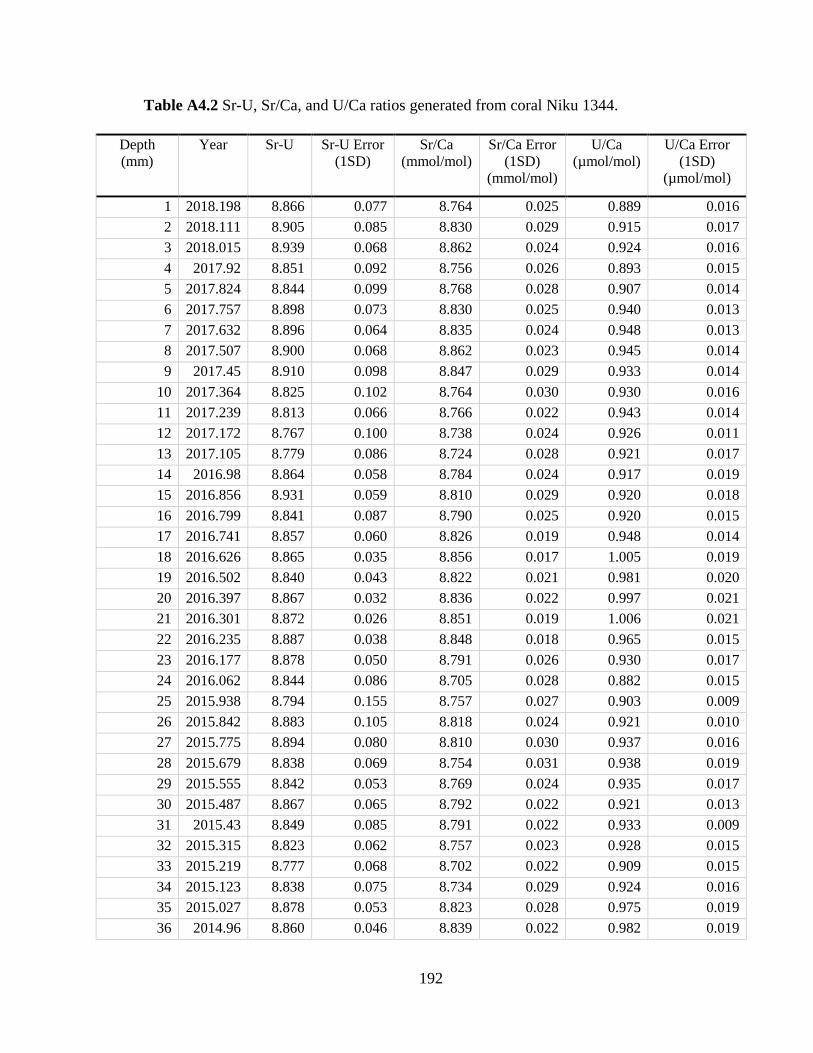
192
Table A4.2 Sr-U, Sr/Ca, and U/Ca ratios generated from coral Niku 1344.
Depth
(mm)
Year Sr-U Sr-U Error
(1SD)
Sr/Ca
(mmol/mol)
Sr/Ca Error
(1SD)
(mmol/mol)
U/Ca
(µmol/mol)
U/Ca Error
(1SD)
(µmol/mol)
1 2018.198 8.866 0.077 8.764 0.025 0.889 0.016
2 2018.111 8.905 0.085 8.830 0.029 0.915 0.017
3 2018.015 8.939 0.068 8.862 0.024 0.924 0.016
4 2017.92 8.851 0.092 8.756 0.026 0.893 0.015
5 2017.824 8.844 0.099 8.768 0.028 0.907 0.014
6 2017.757 8.898 0.073 8.830 0.025 0.940 0.013
7 2017.632 8.896 0.064 8.835 0.024 0.948 0.013
8 2017.507 8.900 0.068 8.862 0.023 0.945 0.014
9 2017.45 8.910 0.098 8.847 0.029 0.933 0.014
10 2017.364 8.825 0.102 8.764 0.030 0.930 0.016
11 2017.239 8.813 0.066 8.766 0.022 0.943 0.014
12 2017.172 8.767 0.100 8.738 0.024 0.926 0.011
13 2017.105 8.779 0.086 8.724 0.028 0.921 0.017
14 2016.98 8.864 0.058 8.784 0.024 0.917 0.019
15 2016.856 8.931 0.059 8.810 0.029 0.920 0.018
16 2016.799 8.841 0.087 8.790 0.025 0.920 0.015
17 2016.741 8.857 0.060 8.826 0.019 0.948 0.014
18 2016.626 8.865 0.035 8.856 0.017 1.005 0.019
19 2016.502 8.840 0.043 8.822 0.021 0.981 0.020
20 2016.397 8.867 0.032 8.836 0.022 0.997 0.021
21 2016.301 8.872 0.026 8.851 0.019 1.006 0.021
22 2016.235 8.887 0.038 8.848 0.018 0.965 0.015
23 2016.177 8.878 0.050 8.791 0.026 0.930 0.017
24 2016.062 8.844 0.086 8.705 0.028 0.882 0.015
25 2015.938 8.794 0.155 8.757 0.027 0.903 0.009
26 2015.842 8.883 0.105 8.818 0.024 0.921 0.010
27 2015.775 8.894 0.080 8.810 0.030 0.937 0.016
28 2015.679 8.838 0.069 8.754 0.031 0.938 0.019
29 2015.555 8.842 0.053 8.769 0.024 0.935 0.017
30 2015.487 8.867 0.065 8.792 0.022 0.921 0.013
31 2015.43 8.849 0.085 8.791 0.022 0.933 0.009
32 2015.315 8.823 0.062 8.757 0.023 0.928 0.015
33 2015.219 8.777 0.068 8.702 0.022 0.909 0.015
34 2015.123 8.838 0.075 8.734 0.029 0.924 0.016
35 2015.027 8.878 0.053 8.823 0.028 0.975 0.019
36 2014.96 8.860 0.046 8.839 0.022 0.982 0.019
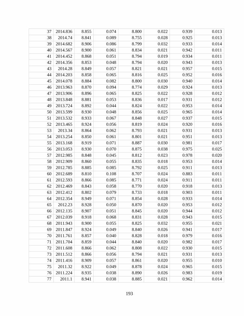
193
37 2014.836 8.855 0.074 8.800 0.022 0.939 0.013
38 2014.74 8.841 0.089 8.755 0.028 0.925 0.013
39 2014.682 8.906 0.086 8.799 0.032 0.933 0.014
40 2014.567 8.900 0.061 8.834 0.021 0.942 0.011
41 2014.452 8.868 0.051 8.794 0.019 0.934 0.011
42 2014.356 8.853 0.048 8.794 0.020 0.943 0.013
43 2014.28 8.849 0.057 8.821 0.021 0.957 0.015
44 2014.203 8.858 0.065 8.816 0.025 0.952 0.016
45 2014.078 8.884 0.082 8.800 0.030 0.940 0.014
46 2013.963 8.870 0.094 8.774 0.029 0.924 0.013
47 2013.906 8.896 0.065 8.825 0.022 0.928 0.012
48 2013.848 8.881 0.053 8.836 0.017 0.931 0.012
49 2013.724 8.892 0.044 8.824 0.022 0.953 0.014
50 2013.599 8.930 0.048 8.856 0.025 0.965 0.014
51 2013.532 8.933 0.067 8.848 0.027 0.937 0.015
52 2013.465 8.924 0.056 8.819 0.024 0.920 0.016
53 2013.34 8.864 0.062 8.793 0.021 0.931 0.013
54 2013.254 8.850 0.061 8.801 0.021 0.951 0.013
55 2013.168 8.919 0.071 8.887 0.030 0.981 0.017
56 2013.053 8.930 0.070 8.875 0.038 0.975 0.025
57 2012.985 8.848 0.045 8.812 0.023 0.978 0.020
58 2012.909 8.860 0.055 8.835 0.018 0.953 0.014
59 2012.785 8.885 0.085 8.792 0.025 0.911 0.013
60 2012.689 8.810 0.108 8.707 0.024 0.883 0.011
61 2012.593 8.866 0.085 8.771 0.024 0.911 0.011
62 2012.469 8.843 0.058 8.770 0.020 0.918 0.013
63 2012.412 8.802 0.079 8.733 0.018 0.903 0.011
64 2012.354 8.949 0.071 8.854 0.028 0.933 0.014
65 2012.23 8.928 0.050 8.870 0.020 0.953 0.012
66 2012.135 8.907 0.051 8.845 0.020 0.944 0.012
67 2012.039 8.918 0.068 8.831 0.028 0.943 0.015
68 2011.943 8.900 0.055 8.825 0.032 0.955 0.021
69 2011.847 8.924 0.049 8.840 0.026 0.941 0.017
70 2011.761 8.857 0.040 8.828 0.018 0.979 0.016
71 2011.704 8.859 0.044 8.840 0.020 0.982 0.017
72 2011.608 8.866 0.062 8.808 0.022 0.930 0.015
73 2011.512 8.866 0.056 8.794 0.021 0.931 0.013
74 2011.416 8.909 0.057 8.861 0.020 0.955 0.010
75 2011.32 8.922 0.049 8.878 0.024 0.965 0.015
76 2011.224 8.935 0.038 8.890 0.026 0.983 0.019
77 2011.1 8.941 0.038 8.885 0.021 0.962 0.014
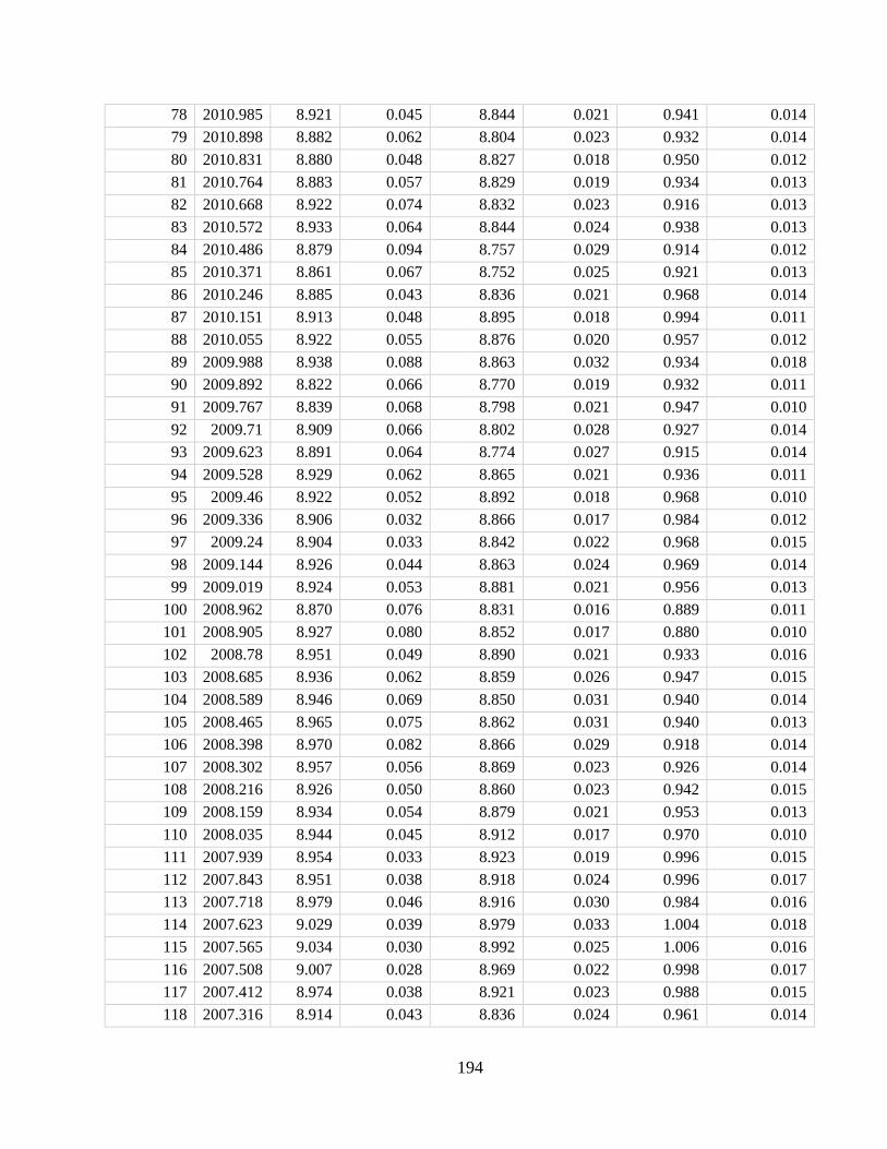
194
78 2010.985 8.921 0.045 8.844 0.021 0.941 0.014
79 2010.898 8.882 0.062 8.804 0.023 0.932 0.014
80 2010.831 8.880 0.048 8.827 0.018 0.950 0.012
81 2010.764 8.883 0.057 8.829 0.019 0.934 0.013
82 2010.668 8.922 0.074 8.832 0.023 0.916 0.013
83 2010.572 8.933 0.064 8.844 0.024 0.938 0.013
84 2010.486 8.879 0.094 8.757 0.029 0.914 0.012
85 2010.371 8.861 0.067 8.752 0.025 0.921 0.013
86 2010.246 8.885 0.043 8.836 0.021 0.968 0.014
87 2010.151 8.913 0.048 8.895 0.018 0.994 0.011
88 2010.055 8.922 0.055 8.876 0.020 0.957 0.012
89 2009.988 8.938 0.088 8.863 0.032 0.934 0.018
90 2009.892 8.822 0.066 8.770 0.019 0.932 0.011
91 2009.767 8.839 0.068 8.798 0.021 0.947 0.010
92 2009.71 8.909 0.066 8.802 0.028 0.927 0.014
93 2009.623 8.891 0.064 8.774 0.027 0.915 0.014
94 2009.528 8.929 0.062 8.865 0.021 0.936 0.011
95 2009.46 8.922 0.052 8.892 0.018 0.968 0.010
96 2009.336 8.906 0.032 8.866 0.017 0.984 0.012
97 2009.24 8.904 0.033 8.842 0.022 0.968 0.015
98 2009.144 8.926 0.044 8.863 0.024 0.969 0.014
99 2009.019 8.924 0.053 8.881 0.021 0.956 0.013
100 2008.962 8.870 0.076 8.831 0.016 0.889 0.011
101 2008.905 8.927 0.080 8.852 0.017 0.880 0.010
102 2008.78 8.951 0.049 8.890 0.021 0.933 0.016
103 2008.685 8.936 0.062 8.859 0.026 0.947 0.015
104 2008.589 8.946 0.069 8.850 0.031 0.940 0.014
105 2008.465 8.965 0.075 8.862 0.031 0.940 0.013
106 2008.398 8.970 0.082 8.866 0.029 0.918 0.014
107 2008.302 8.957 0.056 8.869 0.023 0.926 0.014
108 2008.216 8.926 0.050 8.860 0.023 0.942 0.015
109 2008.159 8.934 0.054 8.879 0.021 0.953 0.013
110 2008.035 8.944 0.045 8.912 0.017 0.970 0.010
111 2007.939 8.954 0.033 8.923 0.019 0.996 0.015
112 2007.843 8.951 0.038 8.918 0.024 0.996 0.017
113 2007.718 8.979 0.046 8.916 0.030 0.984 0.016
114 2007.623 9.029 0.039 8.979 0.033 1.004 0.018
115 2007.565 9.034 0.030 8.992 0.025 1.006 0.016
116 2007.508 9.007 0.028 8.969 0.022 0.998 0.017
117 2007.412 8.974 0.038 8.921 0.023 0.988 0.015
118 2007.316 8.914 0.043 8.836 0.024 0.961 0.014
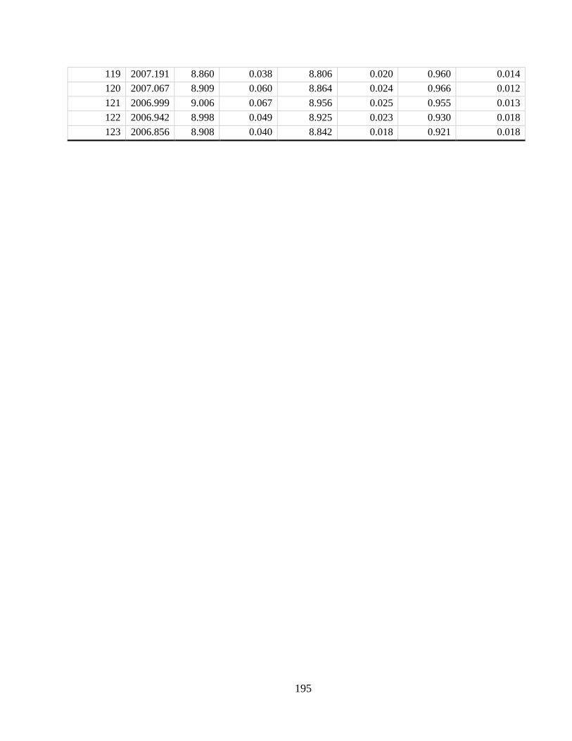
195
119 2007.191 8.860 0.038 8.806 0.020 0.960 0.014
120 2007.067 8.909 0.060 8.864 0.024 0.966 0.012
121 2006.999 9.006 0.067 8.956 0.025 0.955 0.013
122 2006.942 8.998 0.049 8.925 0.023 0.930 0.018
123 2006.856 8.908 0.040 8.842 0.018 0.921 0.018
196
A4.3 References
Branson O, Fehrenbacher JS, Vetter L, Sadekov AY, Eggins SM, Spero HJ (2019) LAtools: A
data analysis package for the reproducible reduction of LA-ICPMS data. Chem Geol 504:83–
95
Decarlo TM, Gaetani GA, Cohen AL, Foster GL, Alpert AE, Stewart JA (2016) Coral Sr-U
thermometry. Paleoceanography 626–638
Hathorne EC, Gagnon A, Felis T, Adkins J, Asami R, Boer W, Caillon N, Case D, Cobb KM,
Douville E, Demenocal P, Eisenhauer A, Garbe-Schönberg D, Geibert W, Goldstein S,
Hughen K, Inoue M, Kawahata H, Kölling M, Cornec FL, Linsley BK, McGregor H V.,
Montagna P, Nurhati IS, Quinn TM, Raddatz J, Rebaubier H, Robinson L, Sadekov A,
Sherrell R, Sinclair D, Tudhope AW, Wei G, Wong H, Wu HC, You CF (2013)
Interlaboratory study for coral Sr/Ca and other element/Ca ratio measurements.
Geochemistry, Geophys Geosystems 14:3730–3750
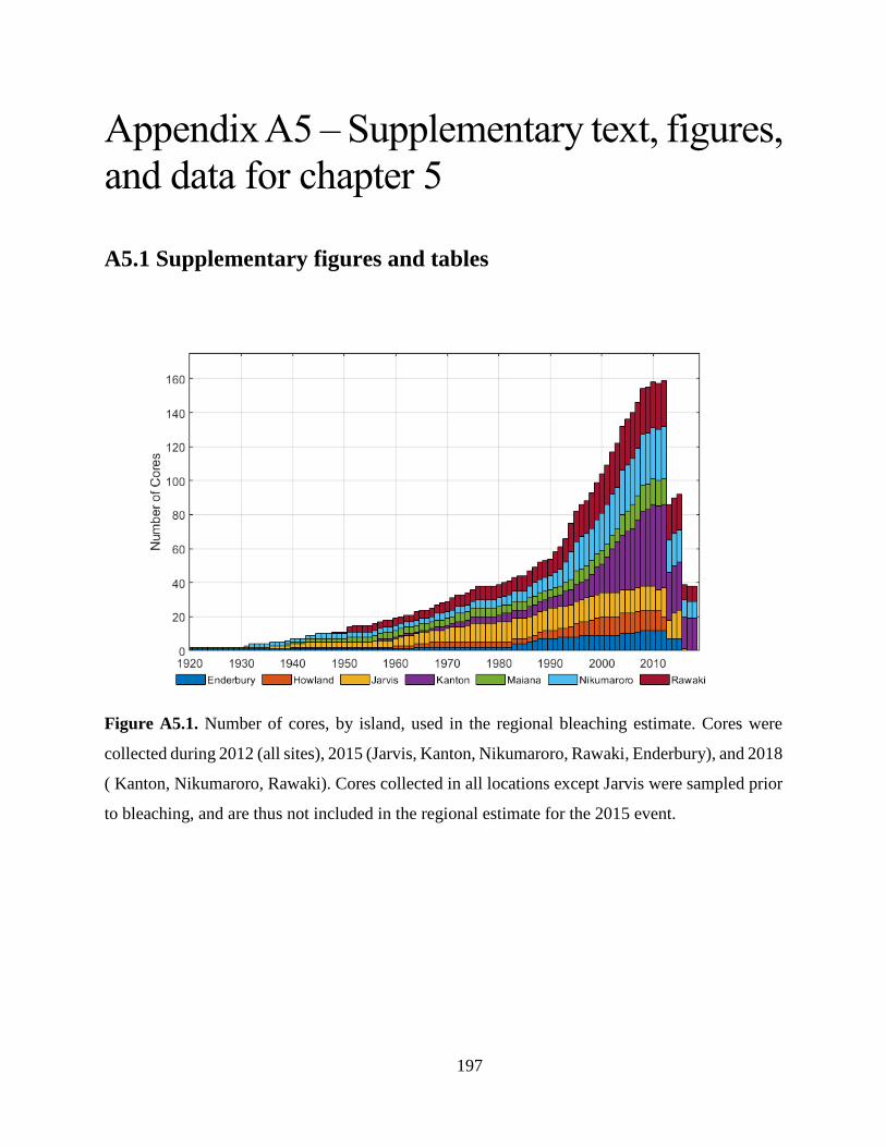
197
Appendix A5 – Supplementary text, figures,
and data for chapter 5
A5.1 Supplementary figures and tables
Figure A5.1. Number of cores, by island, used in the regional bleaching estimate. Cores were
collected during 2012 (all sites), 2015 (Jarvis, Kanton, Nikumaroro, Rawaki, Enderbury), and 2018
( Kanton, Nikumaroro, Rawaki). Cores collected in all locations except Jarvis were sampled prior
to bleaching, and are thus not included in the regional estimate for the 2015 event.
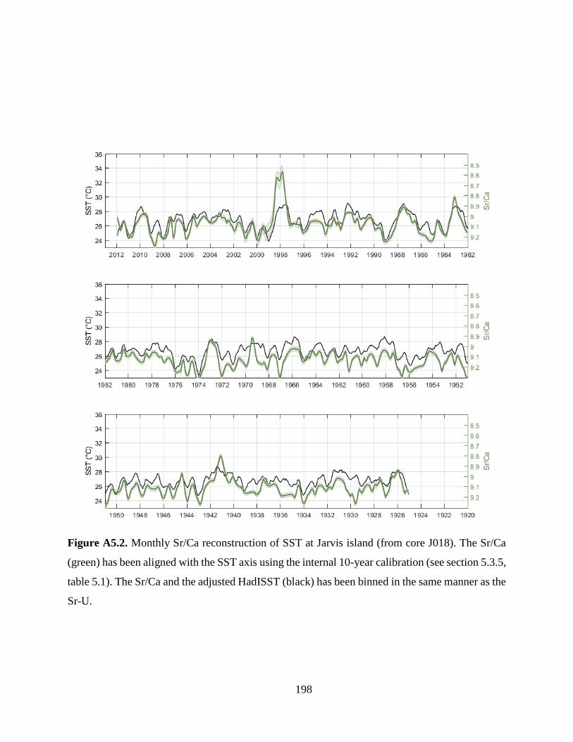
198
Figure A5.2. Monthly Sr/Ca reconstruction of SST at Jarvis island (from core J018). The Sr/Ca
(green) has been aligned with the SST axis using the internal 10-year calibration (see section 5.3.5,
table 5.1). The Sr/Ca and the adjusted HadISST (black) has been binned in the same manner as the
Sr-U.
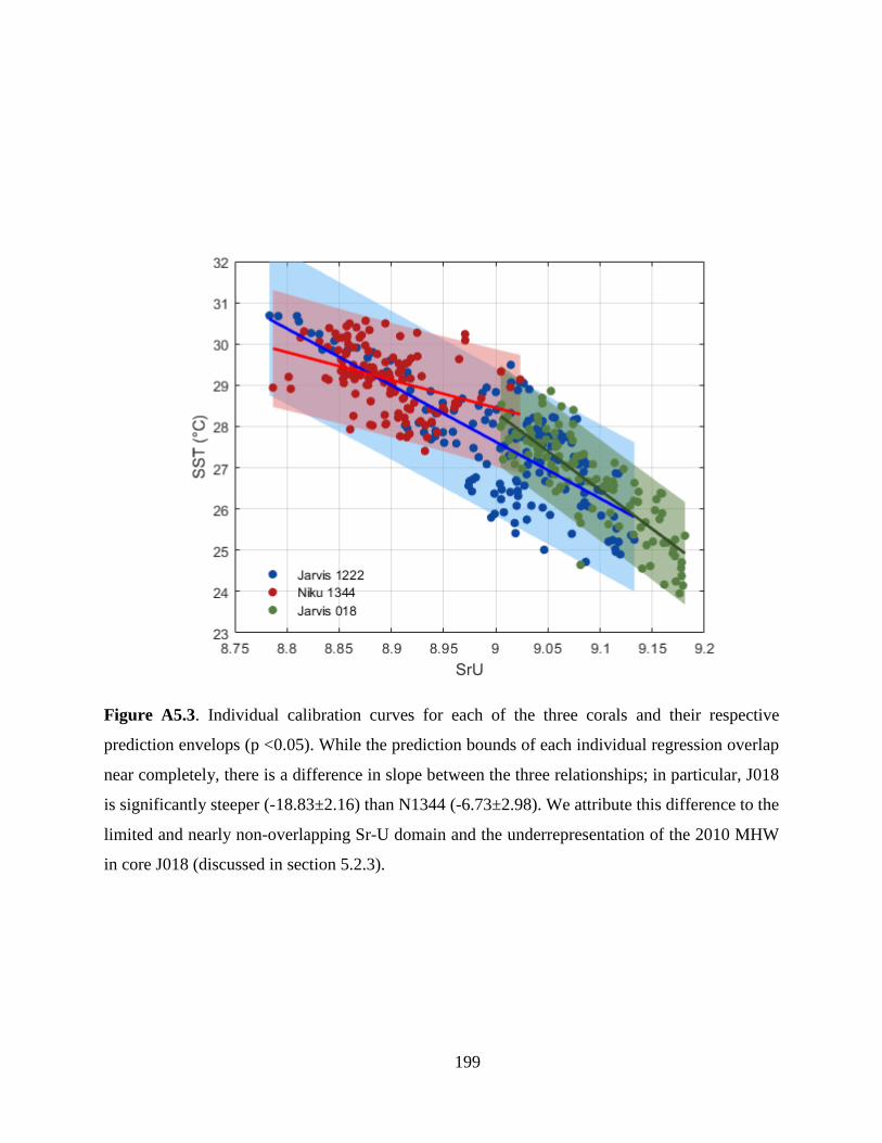
199
Figure A5.3. Individual calibration curves for each of the three corals and their respective
prediction envelops (p <0.05). While the prediction bounds of each individual regression overlap
near completely, there is a difference in slope between the three relationships; in particular, J018
is significantly steeper (-18.83±2.16) than N1344 (-6.73±2.98). We attribute this difference to the
limited and nearly non-overlapping Sr-U domain and the underrepresentation of the 2010 MHW
in core J018 (discussed in section 5.2.3).
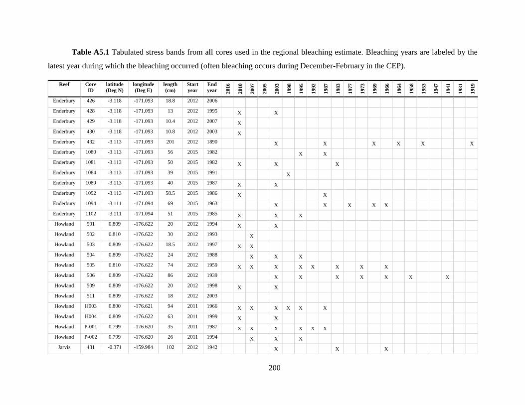
200
Table A5.1 Tabulated stress bands from all cores used in the regional bleaching estimate. Bleaching years are labeled by the
latest year during which the bleaching occurred (often bleaching occurs during December-February in the CEP).
Reef Core
ID
latitude
(Deg N)
longitude
(Deg E)
length
(cm)
Start
year
End
year 2016
2010
2007
2005
2003
1998
1995
1992
1987
1983
1977
1973
1969
1966
1964
1958
1
953
1947
1941
1931
1919
Enderbury 426 -3.118 -171.093 18.8 2012 2006
Enderbury 428 -3.118 -171.093 13 2012 1995 X X
Enderbury 429 -3.118 -171.093 10.4 2012 2007 X
Enderbury 430 -3.118 -171.093 10.8 2012 2003 X
Enderbury 432 -3.113 -171.093 201 2012 1890 X X X X X X
Enderbury 1080 -3.113 -171.093 56 2015 1982 X X
Enderbury 1081 -3.113 -171.093 50 2015 1982 X X X
Enderbury 1084 -3.113 -171.093 39 2015 1991 X
Enderbury 1089 -3.113 -171.093 40 2015 1987 X X
Enderbury 1092 -3.113 -171.093 58.5 2015 1986 X X
Enderbury 1094 -3.111 -171.094 69 2015 1963 X X X X X
Enderbury 1102 -3.111 -171.094 51 2015 1985 X X X
Howland 501 0.809 -176.622 20 2012 1994 X X
Howland 502 0.810 -176.622 30 2012 1993 X
Howland 503 0.809 -176.622 18.5 2012 1997 X X
Howland 504 0.809 -176.622 24 2012 1988 X X X
Howland 505 0.810 -176.622 74 2012 1959 X X X X X X X X
Howland 506 0.809 -176.622 86 2012 1939 X X X X X X X
Howland 509 0.809 -176.622 20 2012 1998 X X
Howland 511 0.809 -176.622 18 2012 2003
Howland H003 0.800 -176.621 94 2011 1966 X X X X X X
Howland H004 0.809 -176.622 63 2011 1999 X X
Howland P-001 0.799 -176.620 35 2011 1987 X X X X X X
Howland P-002 0.799 -176.620 26 2011 1994 X X X
Jarvis 481 -0.371 -159.984 102 2012 1942 X X X
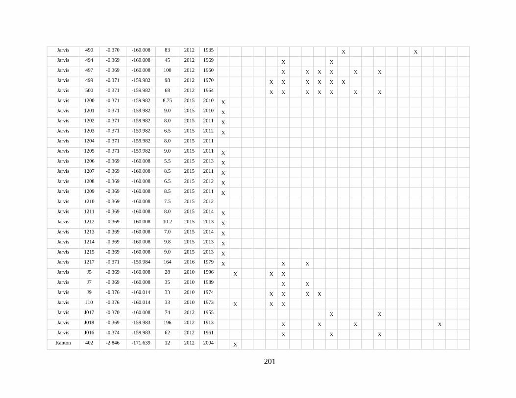
201
Jarvis 490 -0.370 -160.008 83 2012 1935 X X
Jarvis 494 -0.369 -160.008 45 2012 1969 X X
Jarvis 497 -0.369 -160.008 100 2012 1960 X X X X X X
Jarvis 499 -0.371 -159.982 98 2012 1970 X X X X X X
Jarvis 500 -0.371 -159.982 68 2012 1964 X X X X X X X
Jarvis 1200 -0.371 -159.982 8.75 2015 2010 X
Jarvis 1201 -0.371 -159.982 9.0 2015 2010 X
Jarvis 1202 -0.371 -159.982 8.0 2015 2011 X
Jarvis 1203 -0.371 -159.982 6.5 2015 2012 X
Jarvis 1204 -0.371 -159.982 8.0 2015 2011
Jarvis 1205 -0.371 -159.982 9.0 2015 2011 X
Jarvis 1206 -0.369 -160.008 5.5 2015 2013 X
Jarvis 1207 -0.369 -160.008 8.5 2015 2011 X
Jarvis 1208 -0.369 -160.008 6.5 2015 2012 X
Jarvis 1209 -0.369 -160.008 8.5 2015 2011 X
Jarvis 1210 -0.369 -160.008 7.5 2015 2012
Jarvis 1211 -0.369 -160.008 8.0 2015 2014 X
Jarvis 1212 -0.369 -160.008 10.2 2015 2013 X
Jarvis 1213 -0.369 -160.008 7.0 2015 2014 X
Jarvis 1214 -0.369 -160.008 9.8 2015 2013 X
Jarvis 1215 -0.369 -160.008 9.0 2015 2013 X
Jarvis 1217 -0.371 -159.984 164 2016 1979 X X X
Jarvis J5 -0.369 -160.008 28 2010 1996 X X X
Jarvis J7 -0.369 -160.008 35 2010 1989 X X
Jarvis J9 -0.376 -160.014 33 2010 1974 X X X X
Jarvis J10 -0.376 -160.014 33 2010 1973 X X X
Jarvis J017 -0.370 -160.008 74 2012 1955 X X
Jarvis J018 -0.369 -159.983 196 2012 1913 X X X X
Jarvis J016 -0.374 -159.983 62 2012 1961 X X X
Kanton 402 -2.846 -171.639 12 2012 2004 X
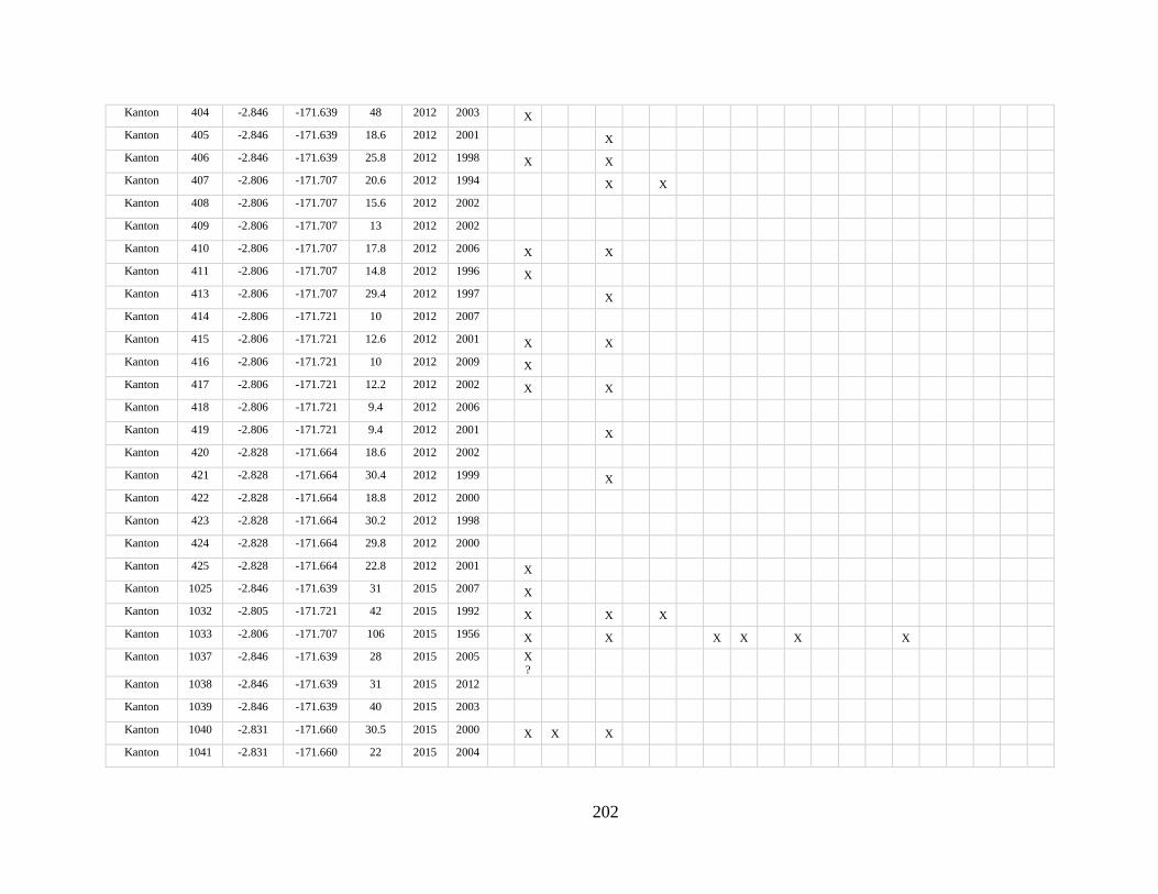
202
Kanton 404 -2.846 -171.639 48 2012 2003 X
Kanton 405 -2.846 -171.639 18.6 2012 2001 X
Kanton 406 -2.846 -171.639 25.8 2012 1998 X X
Kanton 407 -2.806 -171.707 20.6 2012 1994 X X
Kanton 408 -2.806 -171.707 15.6 2012 2002
Kanton 409 -2.806 -171.707 13 2012 2002
Kanton 410 -2.806 -171.707 17.8 2012 2006 X X
Kanton 411 -2.806 -171.707 14.8 2012 1996 X
Kanton 413 -2.806 -171.707 29.4 2012 1997 X
Kanton 414 -2.806 -171.721 10 2012 2007
Kanton 415 -2.806 -171.721 12.6 2012 2001 X X
Kanton 416 -2.806 -171.721 10 2012 2009 X
Kanton 417 -2.806 -171.721 12.2 2012 2002 X X
Kanton 418 -2.806 -171.721 9.4 2012 2006
Kanton 419 -2.806 -171.721 9.4 2012 2001 X
Kanton 420 -2.828 -171.664 18.6 2012 2002
Kanton 421 -2.828 -171.664 30.4 2012 1999 X
Kanton 422 -2.828 -171.664 18.8 2012 2000
Kanton 423 -2.828 -171.664 30.2 2012 1998
Kanton 424 -2.828 -171.664 29.8 2012 2000
Kanton 425 -2.828 -171.664 22.8 2012 2001 X
Kanton 1025 -2.846 -171.639 31 2015 2007 X
Kanton 1032 -2.805 -171.721 42 2015 1992 X X X
Kanton 1033 -2.806 -171.707 106 2015 1956 X X X X X X
Kanton 1037 -2.846 -171.639 28 2015 2005 X?
Kanton 1038 -2.846 -171.639 31 2015 2012
Kanton 1039 -2.846 -171.639 40 2015 2003
Kanton 1040 -2.831 -171.660 30.5 2015 2000 X X X
Kanton 1041 -2.831 -171.660 22 2015 2004
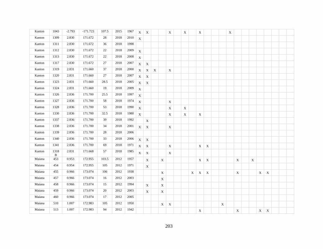
203
Kanton 1043 -2.793 -171.723 107.5 2015 1967 X X X X X X
Kanton 1309 2.830 171.672 28 2018 2010 X
Kanton 1311 2.830 171.672 36 2018 1998
Kanton 1312 2.830 171.672 22 2018 2009 X
Kanton 1313 2.830 171.672 22 2018 2008 X
Kanton 1317 2.830 171.672 27 2018 2007 X X
Kanton 1319 2.831 171.660 37 2018 2000 X X X X
Kanton 1320 2.831 171.660 27 2018 2007 X X
Kanton 1323 2.831 171.660 28.5 2018 2005 X X
Kanton 1324 2.831 171.660 19 2018 2009 X
Kanton 1326 2.836 171.700 25.5 2018 1997 X
Kanton 1327 2.836 171.700 58 2018 1974 X X
Kanton 1328 2.836 171.700 53 2018 1990 X X X
Kanton 1330 2.836 171.700 32.5 2018 1980 X X X X
Kanton 1337 2.836 171.700 39 2018 1992 X
Kanton 1338 2.836 171.700 34 2018 2001 X X X
Kanton 1339 2.836 171.700 28 2018 2006
Kanton 1340 2.836 171.700 33 2018 2006 X X
Kanton 1341 2.836 171.700 69 2018 1971 X X X X X
Kanton 1318
B
2.831 171.668 57 2018 1985 X X X
Maiana 453 0.953 172.955 103.5 2012 1957 X X X X X X
Maiana 454 0.954 172.955 105 2012 1971 X
Maiana 455 0.966 173.074 106 2012 1938 X X X X X X X
Maiana 457 0.966 173.074 16 2012 2003 X
Maiana 458 0.966 173.074 15 2012 1994 X X
Maiana 459 0.966 173.074 20 2012 2003 X X
Maiana 460 0.966 173.074 17 2012 2005
Maiana 510 1.007 172.983 105 2012 1950 X X X
Maiana 513 1.007 172.983 94 2012 1942 X X X X
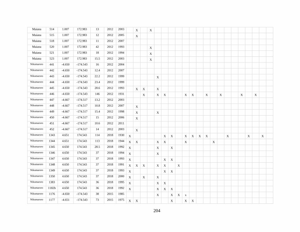
204
Maiana 514 1.007 172.983 13 2012 2003 X X
Maiana 515 1.007 172.983 12 2012 2005 X
Maiana 518 1.007 172.983 11 2012 2007
Maiana 520 1.007 172.983 42 2012 1993 X
Maiana 521 1.007 172.983 18 2012 1994 X
Maiana 523 1.007 172.983 15.5 2012 2003 X
Nikumaroro 441 -4.650 -174.543 16 2012 2004
Nikumaroro 442 -4.650 -174.543 12.4 2012 2007
Nikumaroro 443 -4.650 -174.543 22.2 2012 1999 X
Nikumaroro 444 -4.650 -174.543 23.4 2012 1999
Nikumaroro 445 -4.650 -174.543 28.6 2012 1993 X X X
Nikumaroro 446 -4.650 -174.543 146 2012 1931 X X X X X X X X X
Nikumaroro 447 -4.667 -174.517 13.2 2012 2003
Nikumaroro 448 -4.667 -174.517 10.8 2012 2007 X
Nikumaroro 449 -4.667 -174.517 15.4 2012 1998 X X
Nikumaroro 450 -4.667 -174.517 15 2012 2006 X
Nikumaroro 451 -4.667 -174.517 10.6 2012 2011
Nikumaroro 452 -4.667 -174.517 14 2012 2003 X
Nikumaroro 1343 4.651 174.543 114 2018 1930 X X X X X X X X X X
Nikumaroro 1344 4.651 174.543 113 2018 1944 X X X X X X
Nikumaroro 1345 4.650 174.543 28.5 2018 1992 X X X
Nikumaroro 1346 4.650 174.543 37 2018 1994 X X
Nikumaroro 1347 4.650 174.543 37 2018 1993 X X X
Nikumaroro 1348 4.650 174.543 37 2018 1991 X X X X X X
Nikumaroro 1349 4.650 174.543 37 2018 1993 X X X
Nikumaroro 1350 4.650 174.543 37 2018 2000 X X X
Nikumaroro 1383 4.650 174.543 36 2018 1995 X X X
Nikumaroro 1182b 4.650 174.543 36 2018 1992 X X X X
Nikumaroro 1176 -4.650 -174.543 38 2015 1985 X X X x
Nikumaroro 1177 -4.651 -174.543 73 2015 1975 X X X X X
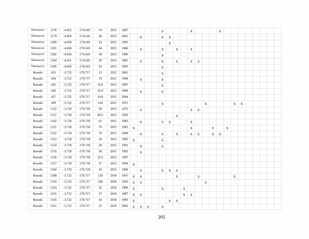
205
Nikumaroro 1178 -4.651 -174.543 74 2015 1967 X X X
Nikumaroro 1179 -4.650 -174.543 28 2015 2001 X X X
Nikumaroro 1180 -4.650 -174.543 33 2015 1993 X
Nikumaroro 1181 -4.650 -174.543 44 2015 1986 X X X X
Nikumaroro 1182 -4.650 -174.543 38 2015 1990 X
Nikumaroro 1184 -4.651 -174.543 39 2015 1981 X X X X X
Nikumaroro 1185 -4.650 -174.543 24 2015 1995 X
Rawaki 433 -3.722 -170.717 15 2012 2001 X
Rawaki 434 -3.722 -170.717 19 2012 1998 X X
Rawaki 435 -3.722 -170.717 16.6 2012 1997 X
Rawaki 436 -3.722 -170.717 20.4 2012 1999 X X
Rawaki 437 -3.722 -170.717 14.6 2012 2004
Rawaki 439 -3.722 -170.717 120 2012 1951 X X X X
Rawaki 1132 -3.720 -170.718 50 2015 1975 X X X
Rawaki 1137 -3.720 -170.718 89.5 2015 1950 X
Rawaki 1142 -3.720 -170.718 61 2015 1983 X X X X
Rawaki 1151 -3.718 -170.718 70 2015 1963 X X X X
Rawaki 1152 -3.718 -170.718 70 2015 1968 X X X X X X X
Rawaki 1153 -3.718 -170.718 34 2015 1993 X X
Rawaki 1154 -3.718 -170.718 28 2015 1993 X X
Rawaki 1155 -3.718 -170.718 36 2015 1992 X
Rawaki 1156 -3.718 -170.718 22.5 2015 1997
Rawaki 1157 -3.718 -170.718 37 2015 1994 X
Rawaki 1160 -3.720 -170.718 43 2015 1990 X X X X
Rawaki 1308 -3.722 -170.717 120 2018 1947 X X X X X
Rawaki 1310 -3.722 -170.717 108 2018 1950 X X X
Rawaki 1314 -3.722 -170.717 32 2018 1990 X X X
Rawaki 1315 -3.722 -170.717 37 2018 1987 X X X X
Rawaki 1316 -3.722 -170.717 34 2018 1993 X X X
Rawaki 1321 -3.722 -170.717 21 2018 2002 X X X X
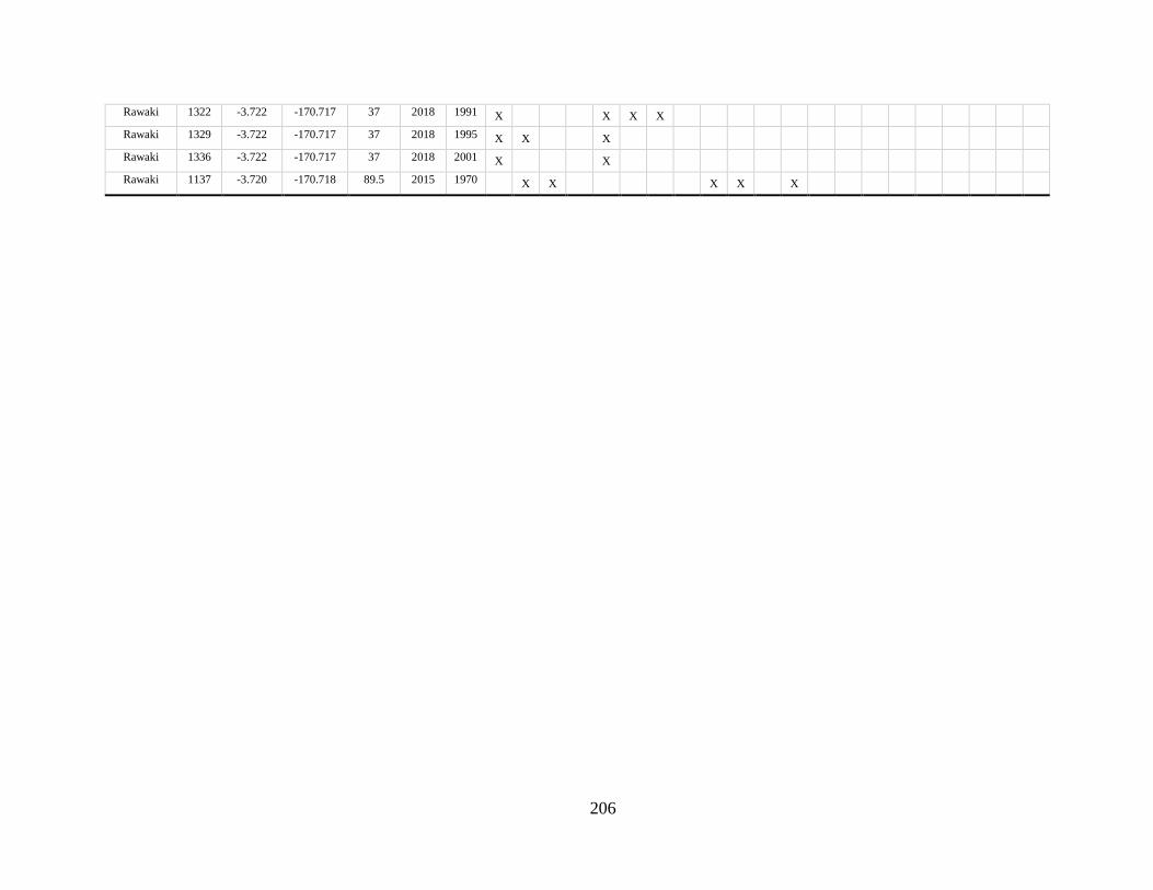
206
Rawaki 1322 -3.722 -170.717 37 2018 1991 X X X X
Rawaki 1329 -3.722 -170.717 37 2018 1995 X X X
Rawaki 1336 -3.722 -170.717 37 2018 2001 X X
Rawaki 1137 -3.720 -170.718 89.5 2015 1970 X X X X X
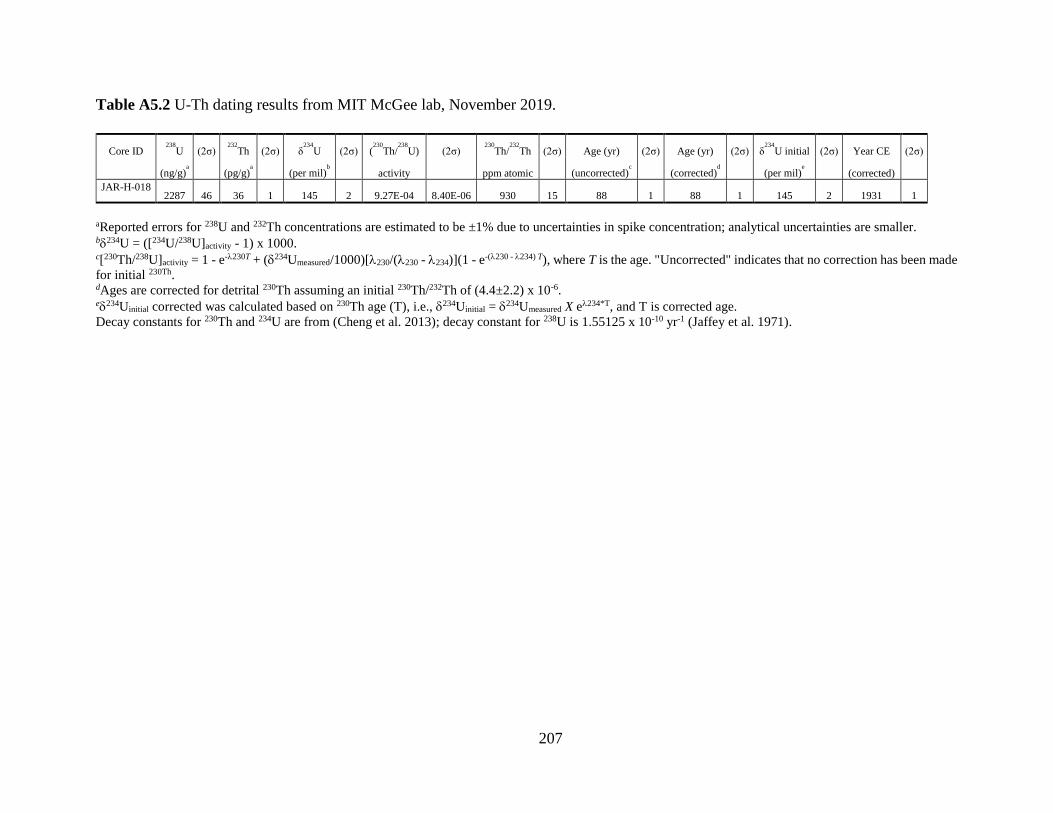
207
Table A5.2 U-Th dating results from MIT McGee lab, November 2019.
Core ID 238U (2σ) 232
Th (2σ) δ234
U (2σ) (230
Th/238
U) (2σ) 230Th/
232Th (2σ) Age (yr) (2σ) Age (yr) (2σ) δ
234U initial (2σ) Year CE (2σ)
(ng/g)a (pg/g)
a (per mil)b activity ppm atomic (uncorrected)
c (corrected)d (per mil)
e (corrected) JAR-H-018
2287 46 36 1 145 2 9.27E-04 8.40E-06 930 15 88 1 88 1 145 2 1931 1
aReported errors for 238U and 232Th concentrations are estimated to be ±1% due to uncertainties in spike concentration; analytical uncertainties are smaller. b234U = ([234U/238U]activity - 1) x 1000. c[230Th/238U]activity = 1 - e-230T + (234Umeasured/1000)[230/(230 - 234)](1 - e-(230 - 234) T), where T is the age. "Uncorrected" indicates that no correction has been made
for initial 230Th. dAges are corrected for detrital 230Th assuming an initial 230Th/232Th of (4.4±2.2) x 10-6. e234Uinitial corrected was calculated based on 230Th age (T), i.e., 234Uinitial = 234Umeasured X e234*T, and T is corrected age.
Decay constants for 230Th and 234U are from (Cheng et al. 2013); decay constant for 238U is 1.55125 x 10⁻¹⁰ yr-1 (Jaffey et al. 1971).
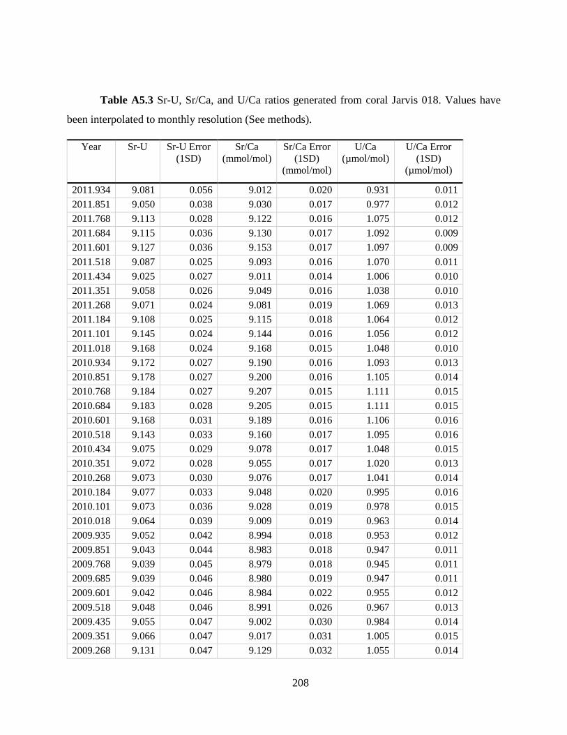
208
Table A5.3 Sr-U, Sr/Ca, and U/Ca ratios generated from coral Jarvis 018. Values have
been interpolated to monthly resolution (See methods).
Year Sr-U Sr-U Error
(1SD)
Sr/Ca
(mmol/mol)
Sr/Ca Error
(1SD)
(mmol/mol)
U/Ca
(µmol/mol)
U/Ca Error
(1SD)
(µmol/mol)
2011.934 9.081 0.056 9.012 0.020 0.931 0.011
2011.851 9.050 0.038 9.030 0.017 0.977 0.012
2011.768 9.113 0.028 9.122 0.016 1.075 0.012
2011.684 9.115 0.036 9.130 0.017 1.092 0.009
2011.601 9.127 0.036 9.153 0.017 1.097 0.009
2011.518 9.087 0.025 9.093 0.016 1.070 0.011
2011.434 9.025 0.027 9.011 0.014 1.006 0.010
2011.351 9.058 0.026 9.049 0.016 1.038 0.010
2011.268 9.071 0.024 9.081 0.019 1.069 0.013
2011.184 9.108 0.025 9.115 0.018 1.064 0.012
2011.101 9.145 0.024 9.144 0.016 1.056 0.012
2011.018 9.168 0.024 9.168 0.015 1.048 0.010
2010.934 9.172 0.027 9.190 0.016 1.093 0.013
2010.851 9.178 0.027 9.200 0.016 1.105 0.014
2010.768 9.184 0.027 9.207 0.015 1.111 0.015
2010.684 9.183 0.028 9.205 0.015 1.111 0.015
2010.601 9.168 0.031 9.189 0.016 1.106 0.016
2010.518 9.143 0.033 9.160 0.017 1.095 0.016
2010.434 9.075 0.029 9.078 0.017 1.048 0.015
2010.351 9.072 0.028 9.055 0.017 1.020 0.013
2010.268 9.073 0.030 9.076 0.017 1.041 0.014
2010.184 9.077 0.033 9.048 0.020 0.995 0.016
2010.101 9.073 0.036 9.028 0.019 0.978 0.015
2010.018 9.064 0.039 9.009 0.019 0.963 0.014
2009.935 9.052 0.042 8.994 0.018 0.953 0.012
2009.851 9.043 0.044 8.983 0.018 0.947 0.011
2009.768 9.039 0.045 8.979 0.018 0.945 0.011
2009.685 9.039 0.046 8.980 0.019 0.947 0.011
2009.601 9.042 0.046 8.984 0.022 0.955 0.012
2009.518 9.048 0.046 8.991 0.026 0.967 0.013
2009.435 9.055 0.047 9.002 0.030 0.984 0.014
2009.351 9.066 0.047 9.017 0.031 1.005 0.015
2009.268 9.131 0.047 9.129 0.032 1.055 0.014
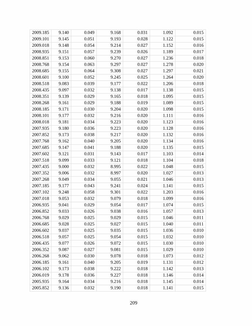
209
2009.185 9.140 0.049 9.168 0.031 1.092 0.015
2009.101 9.145 0.051 9.193 0.028 1.122 0.015
2009.018 9.148 0.054 9.214 0.027 1.152 0.016
2008.935 9.151 0.057 9.239 0.026 1.189 0.017
2008.851 9.153 0.060 9.270 0.027 1.236 0.018
2008.768 9.154 0.063 9.297 0.027 1.278 0.020
2008.685 9.155 0.064 9.308 0.027 1.297 0.021
2008.601 9.100 0.052 9.245 0.025 1.264 0.020
2008.518 9.083 0.039 9.177 0.022 1.206 0.018
2008.435 9.097 0.032 9.138 0.017 1.138 0.015
2008.351 9.139 0.029 9.165 0.018 1.095 0.015
2008.268 9.161 0.029 9.188 0.019 1.089 0.015
2008.185 9.171 0.030 9.204 0.020 1.098 0.015
2008.101 9.177 0.032 9.216 0.020 1.111 0.016
2008.018 9.181 0.034 9.223 0.020 1.123 0.016
2007.935 9.180 0.036 9.223 0.020 1.128 0.016
2007.852 9.173 0.038 9.217 0.020 1.132 0.016
2007.768 9.162 0.040 9.205 0.020 1.134 0.016
2007.685 9.147 0.041 9.188 0.020 1.135 0.015
2007.602 9.121 0.031 9.143 0.017 1.103 0.014
2007.518 9.099 0.033 9.121 0.018 1.104 0.018
2007.435 9.000 0.032 8.995 0.022 1.048 0.015
2007.352 9.006 0.032 8.997 0.020 1.027 0.013
2007.268 9.049 0.034 9.055 0.021 1.046 0.013
2007.185 9.177 0.043 9.241 0.024 1.141 0.015
2007.102 9.248 0.058 9.301 0.022 1.203 0.016
2007.018 9.053 0.032 9.079 0.018 1.099 0.016
2006.935 9.041 0.029 9.054 0.017 1.074 0.015
2006.852 9.033 0.026 9.038 0.016 1.057 0.013
2006.768 9.029 0.025 9.029 0.015 1.046 0.011
2006.685 9.028 0.025 9.027 0.015 1.040 0.011
2006.602 9.037 0.025 9.035 0.015 1.036 0.010
2006.518 9.057 0.025 9.054 0.015 1.032 0.010
2006.435 9.077 0.026 9.072 0.015 1.030 0.010
2006.352 9.087 0.027 9.081 0.015 1.029 0.010
2006.268 9.062 0.030 9.078 0.018 1.073 0.012
2006.185 9.161 0.040 9.205 0.019 1.131 0.012
2006.102 9.173 0.038 9.222 0.018 1.142 0.013
2006.019 9.178 0.036 9.227 0.018 1.146 0.014
2005.935 9.164 0.034 9.216 0.018 1.145 0.014
2005.852 9.136 0.032 9.190 0.018 1.141 0.015
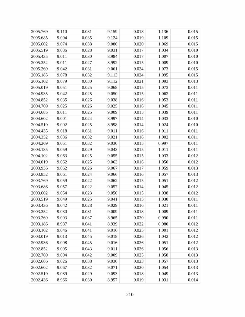
210
2005.769 9.110 0.031 9.159 0.018 1.136 0.015
2005.685 9.094 0.035 9.124 0.019 1.109 0.015
2005.602 9.074 0.038 9.080 0.020 1.069 0.015
2005.519 9.036 0.028 9.031 0.017 1.034 0.010
2005.435 9.011 0.030 8.984 0.017 1.007 0.010
2005.352 9.011 0.027 8.992 0.015 1.009 0.010
2005.269 9.042 0.031 9.061 0.024 1.073 0.015
2005.185 9.078 0.032 9.113 0.024 1.095 0.015
2005.102 9.079 0.030 9.112 0.021 1.093 0.013
2005.019 9.051 0.025 9.068 0.015 1.073 0.011
2004.935 9.042 0.025 9.050 0.015 1.062 0.011
2004.852 9.035 0.026 9.038 0.016 1.053 0.011
2004.769 9.025 0.026 9.025 0.016 1.045 0.011
2004.685 9.011 0.025 9.009 0.015 1.039 0.011
2004.602 9.001 0.024 8.997 0.014 1.033 0.010
2004.519 9.002 0.025 8.998 0.014 1.024 0.010
2004.435 9.018 0.031 9.011 0.016 1.011 0.011
2004.352 9.036 0.032 9.021 0.016 1.002 0.011
2004.269 9.051 0.032 9.030 0.015 0.997 0.011
2004.185 9.059 0.029 9.043 0.015 1.011 0.011
2004.102 9.063 0.025 9.055 0.015 1.033 0.012
2004.019 9.062 0.025 9.063 0.016 1.050 0.012
2003.936 9.062 0.026 9.067 0.017 1.059 0.013
2003.852 9.061 0.024 9.066 0.016 1.057 0.013
2003.769 9.059 0.022 9.062 0.015 1.051 0.012
2003.686 9.057 0.022 9.057 0.014 1.045 0.012
2003.602 9.054 0.023 9.050 0.015 1.038 0.012
2003.519 9.049 0.025 9.041 0.015 1.030 0.011
2003.436 9.042 0.028 9.029 0.016 1.021 0.011
2003.352 9.030 0.031 9.009 0.018 1.009 0.011
2003.269 9.003 0.037 8.965 0.020 0.990 0.011
2003.186 8.987 0.041 8.939 0.022 0.980 0.012
2003.102 9.046 0.041 9.016 0.025 1.001 0.012
2003.019 9.013 0.045 9.018 0.026 1.042 0.012
2002.936 9.008 0.045 9.016 0.026 1.051 0.012
2002.852 9.005 0.043 9.011 0.026 1.056 0.013
2002.769 9.004 0.042 9.009 0.025 1.058 0.013
2002.686 9.026 0.038 9.030 0.023 1.057 0.013
2002.602 9.067 0.032 9.071 0.020 1.054 0.013
2002.519 9.089 0.029 9.093 0.018 1.049 0.013
2002.436 8.966 0.030 8.957 0.019 1.031 0.014
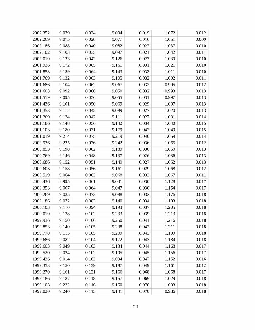
211
2002.352 9.079 0.034 9.094 0.019 1.072 0.012
2002.269 9.075 0.028 9.077 0.016 1.051 0.009
2002.186 9.088 0.040 9.082 0.022 1.037 0.010
2002.102 9.103 0.035 9.097 0.021 1.042 0.011
2002.019 9.133 0.042 9.126 0.023 1.039 0.010
2001.936 9.172 0.065 9.161 0.031 1.021 0.010
2001.853 9.159 0.064 9.143 0.032 1.011 0.010
2001.769 9.132 0.063 9.105 0.032 1.002 0.011
2001.686 9.104 0.062 9.067 0.032 0.995 0.012
2001.603 9.092 0.060 9.050 0.032 0.993 0.013
2001.519 9.095 0.056 9.055 0.031 0.997 0.013
2001.436 9.101 0.050 9.069 0.029 1.007 0.013
2001.353 9.112 0.045 9.089 0.027 1.020 0.013
2001.269 9.124 0.042 9.111 0.027 1.031 0.014
2001.186 9.148 0.056 9.142 0.034 1.040 0.015
2001.103 9.180 0.071 9.179 0.042 1.049 0.015
2001.019 9.214 0.075 9.219 0.040 1.059 0.014
2000.936 9.235 0.076 9.242 0.036 1.065 0.012
2000.853 9.190 0.062 9.189 0.030 1.050 0.013
2000.769 9.146 0.048 9.137 0.026 1.036 0.013
2000.686 9.152 0.051 9.149 0.027 1.052 0.013
2000.603 9.158 0.056 9.161 0.029 1.068 0.012
2000.519 9.064 0.062 9.068 0.032 1.067 0.011
2000.436 8.995 0.061 9.031 0.030 1.128 0.017
2000.353 9.007 0.064 9.047 0.030 1.154 0.017
2000.269 9.035 0.073 9.088 0.032 1.176 0.018
2000.186 9.072 0.083 9.140 0.034 1.193 0.018
2000.103 9.110 0.094 9.193 0.037 1.205 0.018
2000.019 9.138 0.102 9.233 0.039 1.213 0.018
1999.936 9.150 0.106 9.250 0.041 1.216 0.018
1999.853 9.140 0.105 9.238 0.042 1.211 0.018
1999.770 9.115 0.105 9.209 0.043 1.199 0.018
1999.686 9.082 0.104 9.172 0.043 1.184 0.018
1999.603 9.049 0.103 9.134 0.044 1.168 0.017
1999.520 9.024 0.102 9.105 0.045 1.156 0.017
1999.436 9.014 0.102 9.094 0.047 1.152 0.016
1999.353 9.150 0.139 9.187 0.049 1.161 0.012
1999.270 9.161 0.121 9.166 0.068 1.068 0.017
1999.186 9.187 0.118 9.157 0.069 1.029 0.018
1999.103 9.222 0.116 9.150 0.070 1.003 0.018
1999.020 9.240 0.115 9.141 0.070 0.986 0.018
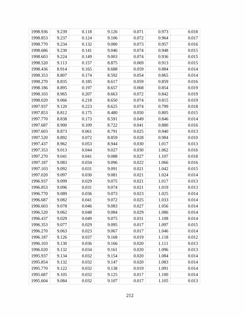
212
1998.936 9.239 0.118 9.126 0.071 0.973 0.018
1998.853 9.237 0.124 9.106 0.072 0.964 0.017
1998.770 9.234 0.132 9.080 0.073 0.957 0.016
1998.686 9.230 0.141 9.046 0.074 0.948 0.015
1998.603 9.224 0.149 9.003 0.074 0.936 0.015
1998.520 9.113 0.157 8.875 0.069 0.913 0.015
1998.436 8.914 0.165 8.688 0.059 0.884 0.014
1998.353 8.807 0.174 8.592 0.054 0.865 0.014
1998.270 8.835 0.185 8.617 0.059 0.859 0.016
1998.186 8.895 0.197 8.657 0.068 0.854 0.019
1998.103 8.965 0.207 8.663 0.072 0.842 0.019
1998.020 9.066 0.218 8.650 0.074 0.815 0.019
1997.937 9.120 0.223 8.625 0.074 0.799 0.018
1997.853 8.812 0.175 8.480 0.050 0.805 0.015
1997.770 8.838 0.173 8.591 0.049 0.846 0.014
1997.687 8.900 0.109 8.722 0.041 0.880 0.016
1997.603 8.873 0.061 8.791 0.025 0.940 0.013
1997.520 8.892 0.072 8.859 0.028 0.984 0.010
1997.437 8.962 0.053 8.944 0.030 1.017 0.013
1997.353 9.013 0.044 9.027 0.030 1.062 0.016
1997.270 9.041 0.041 9.088 0.027 1.107 0.018
1997.187 9.083 0.034 9.096 0.022 1.066 0.016
1997.103 9.092 0.031 9.091 0.021 1.042 0.015
1997.020 9.097 0.030 9.081 0.021 1.024 0.014
1996.937 9.099 0.029 9.075 0.021 1.017 0.013
1996.853 9.096 0.031 9.074 0.021 1.019 0.013
1996.770 9.089 0.036 9.073 0.023 1.025 0.014
1996.687 9.082 0.041 9.072 0.025 1.033 0.014
1996.603 9.078 0.046 9.083 0.027 1.056 0.014
1996.520 9.062 0.048 9.084 0.029 1.086 0.014
1996.437 9.029 0.049 9.075 0.031 1.108 0.014
1996.353 9.077 0.029 9.095 0.017 1.097 0.015
1996.270 9.063 0.023 9.067 0.017 1.046 0.014
1996.187 9.126 0.037 9.168 0.019 1.118 0.012
1996.103 9.130 0.036 9.166 0.020 1.111 0.013
1996.020 9.132 0.034 9.161 0.020 1.096 0.013
1995.937 9.134 0.032 9.154 0.020 1.084 0.014
1995.854 9.132 0.032 9.147 0.020 1.083 0.014
1995.770 9.122 0.032 9.138 0.019 1.091 0.014
1995.687 9.105 0.032 9.125 0.017 1.100 0.014
1995.604 9.084 0.032 9.107 0.017 1.105 0.013
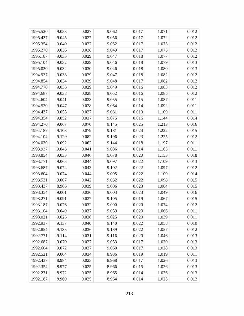
213
1995.520 9.053 0.027 9.062 0.017 1.071 0.012
1995.437 9.045 0.027 9.056 0.017 1.072 0.012
1995.354 9.040 0.027 9.052 0.017 1.073 0.012
1995.270 9.036 0.028 9.049 0.017 1.075 0.012
1995.187 9.033 0.029 9.047 0.018 1.077 0.012
1995.104 9.032 0.029 9.046 0.018 1.079 0.013
1995.020 9.032 0.030 9.046 0.018 1.080 0.013
1994.937 9.033 0.029 9.047 0.018 1.082 0.012
1994.854 9.034 0.029 9.048 0.017 1.082 0.012
1994.770 9.036 0.029 9.049 0.016 1.083 0.012
1994.687 9.038 0.028 9.052 0.016 1.085 0.012
1994.604 9.041 0.028 9.055 0.015 1.087 0.011
1994.520 9.047 0.028 9.064 0.014 1.092 0.011
1994.437 9.055 0.027 9.081 0.013 1.109 0.011
1994.354 9.052 0.037 9.075 0.016 1.144 0.014
1994.270 9.067 0.070 9.145 0.025 1.213 0.016
1994.187 9.103 0.079 9.181 0.024 1.222 0.015
1994.104 9.129 0.082 9.196 0.023 1.225 0.012
1994.020 9.092 0.062 9.144 0.018 1.197 0.011
1993.937 9.045 0.041 9.086 0.014 1.163 0.011
1993.854 9.033 0.046 9.078 0.020 1.153 0.018
1993.771 9.063 0.044 9.097 0.022 1.109 0.013
1993.687 9.074 0.043 9.102 0.022 1.097 0.012
1993.604 9.074 0.044 9.095 0.022 1.100 0.014
1993.521 9.007 0.042 9.032 0.022 1.098 0.015
1993.437 8.986 0.039 9.006 0.023 1.084 0.015
1993.354 9.001 0.036 9.003 0.023 1.049 0.016
1993.271 9.091 0.027 9.105 0.019 1.067 0.015
1993.187 9.076 0.032 9.090 0.020 1.074 0.012
1993.104 9.049 0.037 9.059 0.020 1.066 0.011
1993.021 9.025 0.038 9.025 0.020 1.039 0.011
1992.937 9.137 0.040 9.140 0.022 1.058 0.010
1992.854 9.135 0.036 9.139 0.022 1.057 0.012
1992.771 9.114 0.031 9.116 0.020 1.046 0.013
1992.687 9.070 0.027 9.053 0.017 1.020 0.013
1992.604 9.072 0.027 9.060 0.017 1.028 0.013
1992.521 9.004 0.034 8.986 0.019 1.019 0.011
1992.437 8.984 0.025 8.968 0.017 1.026 0.013
1992.354 8.977 0.025 8.966 0.015 1.026 0.013
1992.271 8.972 0.025 8.965 0.014 1.026 0.013
1992.187 8.969 0.025 8.964 0.014 1.025 0.012
214
1992.104 8.969 0.025 8.964 0.013 1.025 0.011
1992.021 8.970 0.025 8.965 0.014 1.025 0.011
1991.937 8.973 0.025 8.966 0.014 1.024 0.011
1991.854 8.978 0.026 8.967 0.014 1.024 0.010
1991.771 9.039 0.029 9.016 0.017 1.014 0.011
1991.688 9.092 0.025 9.105 0.016 1.070 0.013
1991.604 9.056 0.029 9.053 0.018 1.047 0.012
1991.521 9.018 0.036 9.025 0.020 1.061 0.013
1991.438 8.997 0.043 9.012 0.023 1.081 0.013
1991.354 9.019 0.049 9.035 0.025 1.094 0.014
1991.271 9.066 0.053 9.085 0.025 1.101 0.014
1991.188 9.145 0.032 9.164 0.017 1.103 0.014
1991.104 9.095 0.032 9.124 0.018 1.110 0.015
1991.021 9.086 0.032 9.107 0.018 1.099 0.014
1990.938 9.082 0.031 9.095 0.018 1.077 0.013
1990.854 9.076 0.031 9.083 0.018 1.061 0.012
1990.771 9.061 0.033 9.064 0.019 1.056 0.012
1990.688 9.042 0.035 9.043 0.021 1.052 0.012
1990.604 9.030 0.037 9.029 0.022 1.049 0.013
1990.521 9.027 0.034 9.024 0.020 1.045 0.010
1990.438 9.022 0.033 9.017 0.019 1.041 0.009
1990.354 9.010 0.033 9.006 0.020 1.039 0.010
1990.271 9.013 0.034 9.007 0.021 1.034 0.010
1990.188 9.045 0.037 9.031 0.022 1.023 0.010
1990.104 9.082 0.040 9.061 0.023 1.016 0.010
1990.021 9.125 0.036 9.096 0.022 1.019 0.011
1989.938 9.154 0.032 9.133 0.020 1.026 0.011
1989.855 9.159 0.038 9.162 0.022 1.059 0.012
1989.771 9.087 0.034 9.084 0.021 1.044 0.012
1989.688 9.121 0.034 9.124 0.021 1.053 0.012
1989.605 9.122 0.036 9.128 0.021 1.062 0.012
1989.521 9.092 0.040 9.098 0.021 1.067 0.011
1989.438 9.096 0.038 9.106 0.021 1.071 0.012
1989.355 9.118 0.040 9.148 0.021 1.098 0.014
1989.271 9.170 0.049 9.232 0.023 1.159 0.016
1989.188 9.188 0.049 9.240 0.023 1.153 0.016
1989.105 9.202 0.048 9.245 0.023 1.140 0.015
1989.021 9.211 0.047 9.248 0.023 1.126 0.015
1988.938 9.214 0.046 9.248 0.022 1.116 0.014
1988.855 9.213 0.045 9.242 0.022 1.110 0.014
1988.771 9.207 0.045 9.227 0.022 1.105 0.014
215
1988.688 9.198 0.044 9.212 0.021 1.101 0.013
1988.605 9.187 0.044 9.205 0.021 1.100 0.013
1988.521 9.160 0.053 9.213 0.020 1.191 0.017
1988.438 9.121 0.040 9.165 0.022 1.134 0.018
1988.355 9.112 0.035 9.137 0.020 1.100 0.014
1988.271 9.115 0.031 9.144 0.019 1.098 0.014
1988.188 9.104 0.031 9.117 0.020 1.073 0.014
1988.105 9.078 0.032 9.066 0.021 1.036 0.014
1988.021 9.050 0.033 9.028 0.022 1.028 0.014
1987.938 9.013 0.033 8.997 0.021 1.027 0.014
1987.855 8.983 0.033 8.973 0.020 1.027 0.014
1987.772 8.968 0.033 8.959 0.018 1.025 0.013
1987.688 8.957 0.034 8.946 0.018 1.020 0.012
1987.605 8.942 0.038 8.925 0.018 1.006 0.011
1987.522 8.930 0.045 8.905 0.019 0.988 0.010
1987.438 8.932 0.049 8.904 0.020 0.982 0.010
1987.355 8.952 0.051 8.920 0.021 0.979 0.010
1987.272 8.979 0.052 8.940 0.022 0.978 0.010
1987.188 9.011 0.044 8.973 0.020 0.979 0.011
1987.105 9.045 0.036 8.996 0.019 0.979 0.012
1987.022 9.071 0.050 8.961 0.025 0.940 0.012
1986.938 9.111 0.053 8.971 0.026 0.919 0.013
1986.855 9.057 0.024 9.038 0.018 1.014 0.016
1986.772 9.058 0.024 9.054 0.016 1.044 0.014
1986.688 9.078 0.024 9.080 0.017 1.052 0.015
1986.605 9.052 0.029 9.053 0.018 1.047 0.011
1986.522 9.055 0.036 9.036 0.020 1.016 0.011
1986.438 9.064 0.043 9.044 0.026 1.024 0.013
1986.355 9.071 0.037 9.073 0.022 1.052 0.012
1986.272 9.144 0.034 9.147 0.020 1.046 0.012
1986.188 9.147 0.034 9.161 0.019 1.060 0.013
1986.105 9.148 0.034 9.168 0.018 1.087 0.014
1986.022 9.147 0.035 9.173 0.018 1.108 0.016
1985.938 9.145 0.035 9.177 0.018 1.125 0.017
1985.855 9.140 0.036 9.180 0.018 1.142 0.017
1985.772 9.135 0.037 9.183 0.019 1.158 0.018
1985.689 9.131 0.039 9.187 0.019 1.173 0.019
1985.605 9.129 0.041 9.192 0.019 1.187 0.019
1985.522 9.132 0.043 9.203 0.020 1.202 0.019
1985.439 9.138 0.047 9.220 0.020 1.217 0.018
1985.355 9.144 0.050 9.235 0.020 1.230 0.017
216
1985.272 9.147 0.052 9.242 0.020 1.235 0.017
1985.189 9.148 0.052 9.242 0.020 1.229 0.015
1985.105 9.149 0.051 9.242 0.020 1.216 0.014
1985.022 9.148 0.049 9.240 0.020 1.200 0.014
1984.939 9.146 0.042 9.228 0.020 1.176 0.014
1984.855 9.140 0.036 9.205 0.021 1.146 0.015
1984.772 9.117 0.035 9.157 0.021 1.110 0.014
1984.689 9.048 0.036 9.058 0.021 1.074 0.013
1984.605 8.999 0.027 9.003 0.018 1.065 0.012
1984.522 9.054 0.037 9.052 0.021 1.051 0.011
1984.439 9.093 0.037 9.096 0.020 1.055 0.012
1984.355 9.112 0.038 9.123 0.020 1.066 0.013
1984.272 9.125 0.039 9.142 0.018 1.094 0.013
1984.189 9.134 0.040 9.157 0.017 1.129 0.013
1984.105 9.139 0.041 9.169 0.016 1.155 0.013
1984.022 9.139 0.042 9.178 0.016 1.159 0.013
1983.939 9.138 0.044 9.187 0.017 1.159 0.013
1983.856 9.136 0.046 9.194 0.020 1.159 0.014
1983.772 9.133 0.048 9.196 0.023 1.159 0.015
1983.689 9.048 0.051 9.116 0.032 1.137 0.019
1983.606 8.972 0.050 9.052 0.033 1.145 0.021
1983.522 8.937 0.042 9.026 0.026 1.189 0.021
1983.439 8.965 0.038 9.029 0.023 1.172 0.020
1983.356 8.958 0.038 8.997 0.023 1.120 0.016
1983.272 8.891 0.040 8.875 0.025 1.028 0.010
1983.189 8.848 0.039 8.825 0.018 0.994 0.009
1983.106 8.866 0.052 8.786 0.019 0.929 0.010
1983.022 8.888 0.038 8.836 0.019 0.973 0.011
1982.939 8.925 0.032 8.903 0.019 1.021 0.011
1982.856 8.960 0.030 8.958 0.018 1.052 0.011
1982.772 8.979 0.030 8.983 0.019 1.060 0.011
1982.689 8.994 0.031 8.999 0.019 1.064 0.011
1982.606 9.007 0.032 9.015 0.020 1.068 0.011
1982.522 9.020 0.033 9.036 0.020 1.079 0.012
1982.439 9.031 0.035 9.063 0.019 1.101 0.012
1982.356 9.046 0.037 9.087 0.019 1.124 0.012
1982.272 9.074 0.040 9.107 0.018 1.141 0.013
1982.189 9.121 0.034 9.139 0.016 1.113 0.013
1982.106 9.133 0.034 9.151 0.016 1.110 0.012
1982.022 9.138 0.034 9.158 0.016 1.108 0.011
1981.939 9.138 0.035 9.158 0.016 1.111 0.011
217
1981.856 9.129 0.038 9.150 0.016 1.124 0.011
1981.773 9.115 0.040 9.137 0.016 1.138 0.011
1981.689 9.095 0.038 9.121 0.016 1.138 0.012
1981.606 9.074 0.030 9.104 0.016 1.120 0.014
1981.523 9.122 0.030 9.129 0.017 1.055 0.012
1981.439 9.014 0.032 9.014 0.018 1.045 0.011
1981.356 9.038 0.031 9.037 0.019 1.056 0.012
1981.273 9.058 0.029 9.052 0.019 1.040 0.012
1981.189 9.102 0.033 9.124 0.020 1.086 0.014
1981.106 9.110 0.035 9.133 0.020 1.095 0.014
1981.023 9.115 0.037 9.140 0.020 1.101 0.014
1980.939 9.118 0.038 9.143 0.020 1.105 0.014
1980.856 9.119 0.039 9.144 0.021 1.106 0.014
1980.773 9.114 0.039 9.141 0.022 1.105 0.015
1980.689 9.101 0.039 9.131 0.024 1.103 0.016
1980.606 9.082 0.039 9.113 0.025 1.098 0.018
1980.523 9.057 0.038 9.088 0.026 1.090 0.018
1980.439 9.002 0.033 8.996 0.019 1.035 0.013
1980.356 9.016 0.033 9.010 0.018 1.021 0.012
1980.273 9.057 0.036 9.093 0.022 1.107 0.017
1980.189 9.063 0.036 9.095 0.022 1.106 0.017
1980.106 9.067 0.036 9.096 0.022 1.105 0.016
1980.023 9.069 0.036 9.097 0.022 1.104 0.016
1979.939 9.070 0.037 9.097 0.022 1.104 0.015
1979.856 9.062 0.038 9.089 0.022 1.103 0.015
1979.773 9.045 0.041 9.072 0.023 1.103 0.015
1979.690 9.028 0.043 9.055 0.023 1.103 0.015
1979.606 9.020 0.044 9.047 0.024 1.103 0.015
1979.523 9.054 0.040 9.071 0.021 1.094 0.012
1979.440 9.077 0.038 9.093 0.020 1.093 0.011
1979.356 9.085 0.038 9.107 0.019 1.103 0.011
1979.273 9.093 0.038 9.118 0.018 1.109 0.012
1979.190 9.102 0.037 9.129 0.019 1.110 0.012
1979.106 9.111 0.037 9.140 0.019 1.111 0.013
1979.023 9.120 0.037 9.150 0.020 1.111 0.013
1978.940 9.125 0.037 9.155 0.020 1.111 0.013
1978.856 9.126 0.036 9.156 0.020 1.111 0.013
1978.773 9.125 0.036 9.153 0.020 1.107 0.013
1978.690 9.122 0.036 9.148 0.021 1.101 0.013
1978.606 9.117 0.035 9.140 0.021 1.092 0.013
1978.523 9.042 0.034 9.044 0.019 1.065 0.011
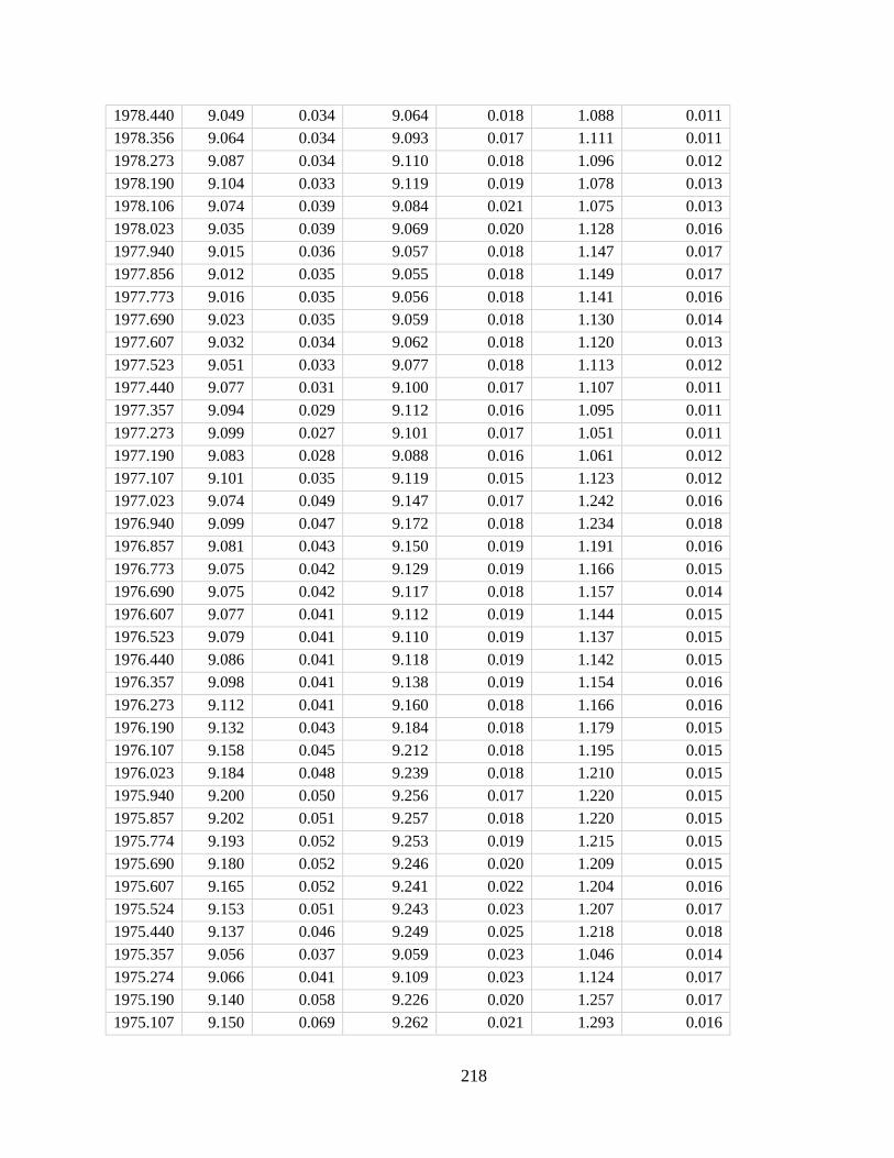
218
1978.440 9.049 0.034 9.064 0.018 1.088 0.011
1978.356 9.064 0.034 9.093 0.017 1.111 0.011
1978.273 9.087 0.034 9.110 0.018 1.096 0.012
1978.190 9.104 0.033 9.119 0.019 1.078 0.013
1978.106 9.074 0.039 9.084 0.021 1.075 0.013
1978.023 9.035 0.039 9.069 0.020 1.128 0.016
1977.940 9.015 0.036 9.057 0.018 1.147 0.017
1977.856 9.012 0.035 9.055 0.018 1.149 0.017
1977.773 9.016 0.035 9.056 0.018 1.141 0.016
1977.690 9.023 0.035 9.059 0.018 1.130 0.014
1977.607 9.032 0.034 9.062 0.018 1.120 0.013
1977.523 9.051 0.033 9.077 0.018 1.113 0.012
1977.440 9.077 0.031 9.100 0.017 1.107 0.011
1977.357 9.094 0.029 9.112 0.016 1.095 0.011
1977.273 9.099 0.027 9.101 0.017 1.051 0.011
1977.190 9.083 0.028 9.088 0.016 1.061 0.012
1977.107 9.101 0.035 9.119 0.015 1.123 0.012
1977.023 9.074 0.049 9.147 0.017 1.242 0.016
1976.940 9.099 0.047 9.172 0.018 1.234 0.018
1976.857 9.081 0.043 9.150 0.019 1.191 0.016
1976.773 9.075 0.042 9.129 0.019 1.166 0.015
1976.690 9.075 0.042 9.117 0.018 1.157 0.014
1976.607 9.077 0.041 9.112 0.019 1.144 0.015
1976.523 9.079 0.041 9.110 0.019 1.137 0.015
1976.440 9.086 0.041 9.118 0.019 1.142 0.015
1976.357 9.098 0.041 9.138 0.019 1.154 0.016
1976.273 9.112 0.041 9.160 0.018 1.166 0.016
1976.190 9.132 0.043 9.184 0.018 1.179 0.015
1976.107 9.158 0.045 9.212 0.018 1.195 0.015
1976.023 9.184 0.048 9.239 0.018 1.210 0.015
1975.940 9.200 0.050 9.256 0.017 1.220 0.015
1975.857 9.202 0.051 9.257 0.018 1.220 0.015
1975.774 9.193 0.052 9.253 0.019 1.215 0.015
1975.690 9.180 0.052 9.246 0.020 1.209 0.015
1975.607 9.165 0.052 9.241 0.022 1.204 0.016
1975.524 9.153 0.051 9.243 0.023 1.207 0.017
1975.440 9.137 0.046 9.249 0.025 1.218 0.018
1975.357 9.056 0.037 9.059 0.023 1.046 0.014
1975.274 9.066 0.041 9.109 0.023 1.124 0.017
1975.190 9.140 0.058 9.226 0.020 1.257 0.017
1975.107 9.150 0.069 9.262 0.021 1.293 0.016
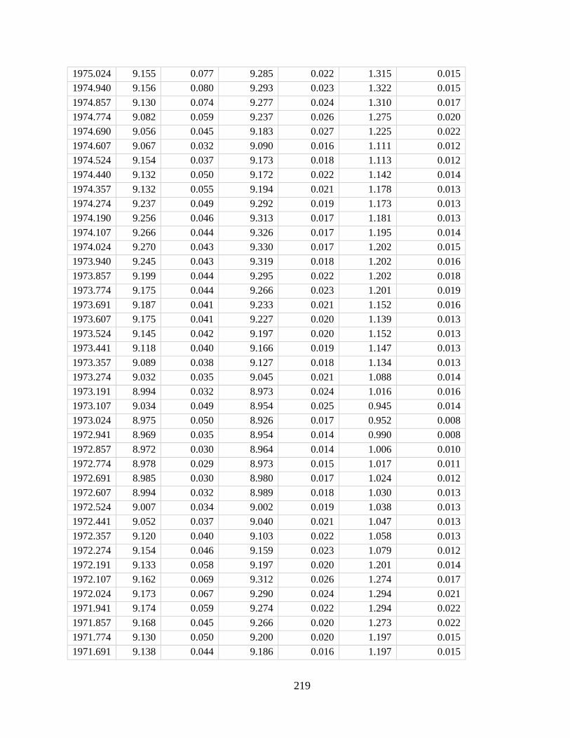
219
1975.024 9.155 0.077 9.285 0.022 1.315 0.015
1974.940 9.156 0.080 9.293 0.023 1.322 0.015
1974.857 9.130 0.074 9.277 0.024 1.310 0.017
1974.774 9.082 0.059 9.237 0.026 1.275 0.020
1974.690 9.056 0.045 9.183 0.027 1.225 0.022
1974.607 9.067 0.032 9.090 0.016 1.111 0.012
1974.524 9.154 0.037 9.173 0.018 1.113 0.012
1974.440 9.132 0.050 9.172 0.022 1.142 0.014
1974.357 9.132 0.055 9.194 0.021 1.178 0.013
1974.274 9.237 0.049 9.292 0.019 1.173 0.013
1974.190 9.256 0.046 9.313 0.017 1.181 0.013
1974.107 9.266 0.044 9.326 0.017 1.195 0.014
1974.024 9.270 0.043 9.330 0.017 1.202 0.015
1973.940 9.245 0.043 9.319 0.018 1.202 0.016
1973.857 9.199 0.044 9.295 0.022 1.202 0.018
1973.774 9.175 0.044 9.266 0.023 1.201 0.019
1973.691 9.187 0.041 9.233 0.021 1.152 0.016
1973.607 9.175 0.041 9.227 0.020 1.139 0.013
1973.524 9.145 0.042 9.197 0.020 1.152 0.013
1973.441 9.118 0.040 9.166 0.019 1.147 0.013
1973.357 9.089 0.038 9.127 0.018 1.134 0.013
1973.274 9.032 0.035 9.045 0.021 1.088 0.014
1973.191 8.994 0.032 8.973 0.024 1.016 0.016
1973.107 9.034 0.049 8.954 0.025 0.945 0.014
1973.024 8.975 0.050 8.926 0.017 0.952 0.008
1972.941 8.969 0.035 8.954 0.014 0.990 0.008
1972.857 8.972 0.030 8.964 0.014 1.006 0.010
1972.774 8.978 0.029 8.973 0.015 1.017 0.011
1972.691 8.985 0.030 8.980 0.017 1.024 0.012
1972.607 8.994 0.032 8.989 0.018 1.030 0.013
1972.524 9.007 0.034 9.002 0.019 1.038 0.013
1972.441 9.052 0.037 9.040 0.021 1.047 0.013
1972.357 9.120 0.040 9.103 0.022 1.058 0.013
1972.274 9.154 0.046 9.159 0.023 1.079 0.012
1972.191 9.133 0.058 9.197 0.020 1.201 0.014
1972.107 9.162 0.069 9.312 0.026 1.274 0.017
1972.024 9.173 0.067 9.290 0.024 1.294 0.021
1971.941 9.174 0.059 9.274 0.022 1.294 0.022
1971.857 9.168 0.045 9.266 0.020 1.273 0.022
1971.774 9.130 0.050 9.200 0.020 1.197 0.015
1971.691 9.138 0.044 9.186 0.016 1.197 0.015
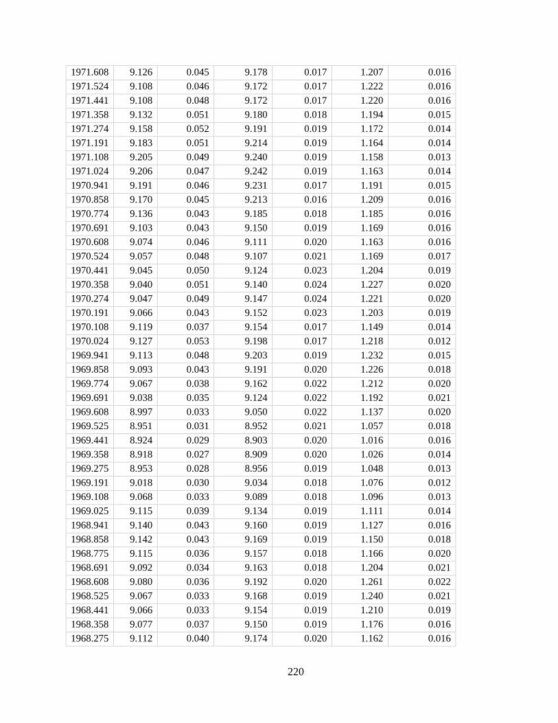
220
1971.608 9.126 0.045 9.178 0.017 1.207 0.016
1971.524 9.108 0.046 9.172 0.017 1.222 0.016
1971.441 9.108 0.048 9.172 0.017 1.220 0.016
1971.358 9.132 0.051 9.180 0.018 1.194 0.015
1971.274 9.158 0.052 9.191 0.019 1.172 0.014
1971.191 9.183 0.051 9.214 0.019 1.164 0.014
1971.108 9.205 0.049 9.240 0.019 1.158 0.013
1971.024 9.206 0.047 9.242 0.019 1.163 0.014
1970.941 9.191 0.046 9.231 0.017 1.191 0.015
1970.858 9.170 0.045 9.213 0.016 1.209 0.016
1970.774 9.136 0.043 9.185 0.018 1.185 0.016
1970.691 9.103 0.043 9.150 0.019 1.169 0.016
1970.608 9.074 0.046 9.111 0.020 1.163 0.016
1970.524 9.057 0.048 9.107 0.021 1.169 0.017
1970.441 9.045 0.050 9.124 0.023 1.204 0.019
1970.358 9.040 0.051 9.140 0.024 1.227 0.020
1970.274 9.047 0.049 9.147 0.024 1.221 0.020
1970.191 9.066 0.043 9.152 0.023 1.203 0.019
1970.108 9.119 0.037 9.154 0.017 1.149 0.014
1970.024 9.127 0.053 9.198 0.017 1.218 0.012
1969.941 9.113 0.048 9.203 0.019 1.232 0.015
1969.858 9.093 0.043 9.191 0.020 1.226 0.018
1969.774 9.067 0.038 9.162 0.022 1.212 0.020
1969.691 9.038 0.035 9.124 0.022 1.192 0.021
1969.608 8.997 0.033 9.050 0.022 1.137 0.020
1969.525 8.951 0.031 8.952 0.021 1.057 0.018
1969.441 8.924 0.029 8.903 0.020 1.016 0.016
1969.358 8.918 0.027 8.909 0.020 1.026 0.014
1969.275 8.953 0.028 8.956 0.019 1.048 0.013
1969.191 9.018 0.030 9.034 0.018 1.076 0.012
1969.108 9.068 0.033 9.089 0.018 1.096 0.013
1969.025 9.115 0.039 9.134 0.019 1.111 0.014
1968.941 9.140 0.043 9.160 0.019 1.127 0.016
1968.858 9.142 0.043 9.169 0.019 1.150 0.018
1968.775 9.115 0.036 9.157 0.018 1.166 0.020
1968.691 9.092 0.034 9.163 0.018 1.204 0.021
1968.608 9.080 0.036 9.192 0.020 1.261 0.022
1968.525 9.067 0.033 9.168 0.019 1.240 0.021
1968.441 9.066 0.033 9.154 0.019 1.210 0.019
1968.358 9.077 0.037 9.150 0.019 1.176 0.016
1968.275 9.112 0.040 9.174 0.020 1.162 0.016
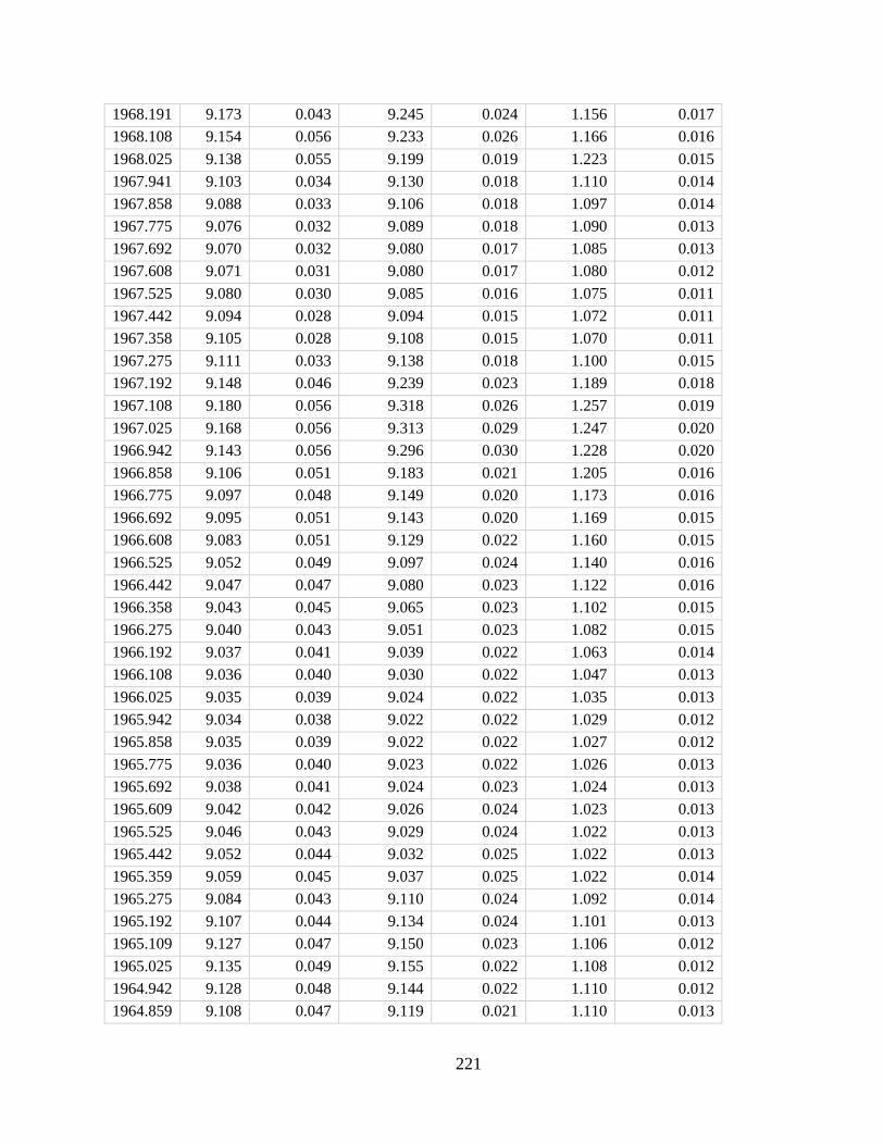
221
1968.191 9.173 0.043 9.245 0.024 1.156 0.017
1968.108 9.154 0.056 9.233 0.026 1.166 0.016
1968.025 9.138 0.055 9.199 0.019 1.223 0.015
1967.941 9.103 0.034 9.130 0.018 1.110 0.014
1967.858 9.088 0.033 9.106 0.018 1.097 0.014
1967.775 9.076 0.032 9.089 0.018 1.090 0.013
1967.692 9.070 0.032 9.080 0.017 1.085 0.013
1967.608 9.071 0.031 9.080 0.017 1.080 0.012
1967.525 9.080 0.030 9.085 0.016 1.075 0.011
1967.442 9.094 0.028 9.094 0.015 1.072 0.011
1967.358 9.105 0.028 9.108 0.015 1.070 0.011
1967.275 9.111 0.033 9.138 0.018 1.100 0.015
1967.192 9.148 0.046 9.239 0.023 1.189 0.018
1967.108 9.180 0.056 9.318 0.026 1.257 0.019
1967.025 9.168 0.056 9.313 0.029 1.247 0.020
1966.942 9.143 0.056 9.296 0.030 1.228 0.020
1966.858 9.106 0.051 9.183 0.021 1.205 0.016
1966.775 9.097 0.048 9.149 0.020 1.173 0.016
1966.692 9.095 0.051 9.143 0.020 1.169 0.015
1966.608 9.083 0.051 9.129 0.022 1.160 0.015
1966.525 9.052 0.049 9.097 0.024 1.140 0.016
1966.442 9.047 0.047 9.080 0.023 1.122 0.016
1966.358 9.043 0.045 9.065 0.023 1.102 0.015
1966.275 9.040 0.043 9.051 0.023 1.082 0.015
1966.192 9.037 0.041 9.039 0.022 1.063 0.014
1966.108 9.036 0.040 9.030 0.022 1.047 0.013
1966.025 9.035 0.039 9.024 0.022 1.035 0.013
1965.942 9.034 0.038 9.022 0.022 1.029 0.012
1965.858 9.035 0.039 9.022 0.022 1.027 0.012
1965.775 9.036 0.040 9.023 0.022 1.026 0.013
1965.692 9.038 0.041 9.024 0.023 1.024 0.013
1965.609 9.042 0.042 9.026 0.024 1.023 0.013
1965.525 9.046 0.043 9.029 0.024 1.022 0.013
1965.442 9.052 0.044 9.032 0.025 1.022 0.013
1965.359 9.059 0.045 9.037 0.025 1.022 0.014
1965.275 9.084 0.043 9.110 0.024 1.092 0.014
1965.192 9.107 0.044 9.134 0.024 1.101 0.013
1965.109 9.127 0.047 9.150 0.023 1.106 0.012
1965.025 9.135 0.049 9.155 0.022 1.108 0.012
1964.942 9.128 0.048 9.144 0.022 1.110 0.012
1964.859 9.108 0.047 9.119 0.021 1.110 0.013
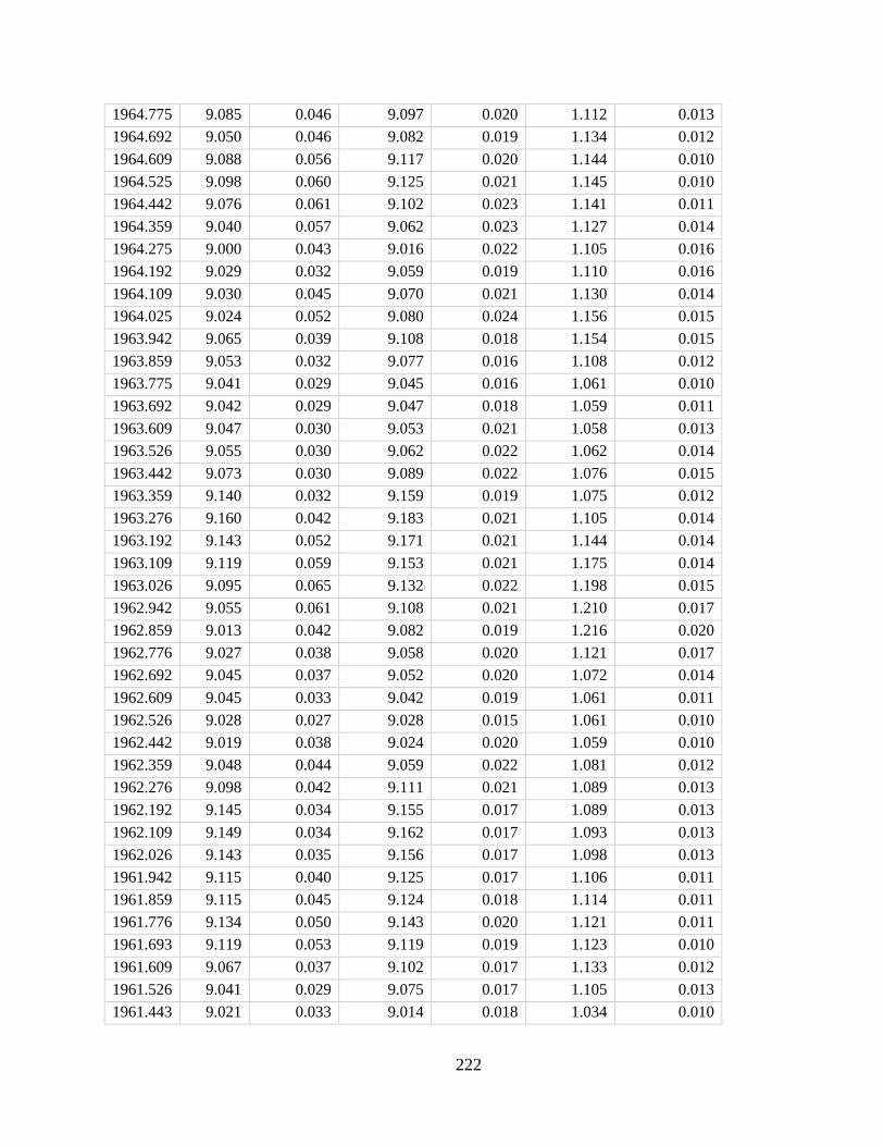
222
1964.775 9.085 0.046 9.097 0.020 1.112 0.013
1964.692 9.050 0.046 9.082 0.019 1.134 0.012
1964.609 9.088 0.056 9.117 0.020 1.144 0.010
1964.525 9.098 0.060 9.125 0.021 1.145 0.010
1964.442 9.076 0.061 9.102 0.023 1.141 0.011
1964.359 9.040 0.057 9.062 0.023 1.127 0.014
1964.275 9.000 0.043 9.016 0.022 1.105 0.016
1964.192 9.029 0.032 9.059 0.019 1.110 0.016
1964.109 9.030 0.045 9.070 0.021 1.130 0.014
1964.025 9.024 0.052 9.080 0.024 1.156 0.015
1963.942 9.065 0.039 9.108 0.018 1.154 0.015
1963.859 9.053 0.032 9.077 0.016 1.108 0.012
1963.775 9.041 0.029 9.045 0.016 1.061 0.010
1963.692 9.042 0.029 9.047 0.018 1.059 0.011
1963.609 9.047 0.030 9.053 0.021 1.058 0.013
1963.526 9.055 0.030 9.062 0.022 1.062 0.014
1963.442 9.073 0.030 9.089 0.022 1.076 0.015
1963.359 9.140 0.032 9.159 0.019 1.075 0.012
1963.276 9.160 0.042 9.183 0.021 1.105 0.014
1963.192 9.143 0.052 9.171 0.021 1.144 0.014
1963.109 9.119 0.059 9.153 0.021 1.175 0.014
1963.026 9.095 0.065 9.132 0.022 1.198 0.015
1962.942 9.055 0.061 9.108 0.021 1.210 0.017
1962.859 9.013 0.042 9.082 0.019 1.216 0.020
1962.776 9.027 0.038 9.058 0.020 1.121 0.017
1962.692 9.045 0.037 9.052 0.020 1.072 0.014
1962.609 9.045 0.033 9.042 0.019 1.061 0.011
1962.526 9.028 0.027 9.028 0.015 1.061 0.010
1962.442 9.019 0.038 9.024 0.020 1.059 0.010
1962.359 9.048 0.044 9.059 0.022 1.081 0.012
1962.276 9.098 0.042 9.111 0.021 1.089 0.013
1962.192 9.145 0.034 9.155 0.017 1.089 0.013
1962.109 9.149 0.034 9.162 0.017 1.093 0.013
1962.026 9.143 0.035 9.156 0.017 1.098 0.013
1961.942 9.115 0.040 9.125 0.017 1.106 0.011
1961.859 9.115 0.045 9.124 0.018 1.114 0.011
1961.776 9.134 0.050 9.143 0.020 1.121 0.011
1961.693 9.119 0.053 9.119 0.019 1.123 0.010
1961.609 9.067 0.037 9.102 0.017 1.133 0.012
1961.526 9.041 0.029 9.075 0.017 1.105 0.013
1961.443 9.021 0.033 9.014 0.018 1.034 0.010
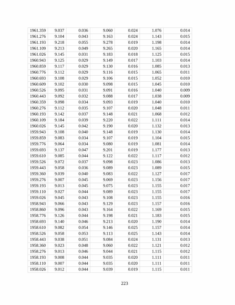
223
1961.359 9.037 0.036 9.060 0.024 1.076 0.014
1961.276 9.104 0.043 9.163 0.024 1.143 0.015
1961.193 9.218 0.055 9.278 0.019 1.198 0.014
1961.109 9.213 0.049 9.265 0.020 1.165 0.014
1961.026 9.145 0.031 9.183 0.018 1.125 0.015
1960.943 9.125 0.029 9.149 0.017 1.103 0.014
1960.859 9.117 0.029 9.130 0.016 1.085 0.013
1960.776 9.112 0.029 9.116 0.015 1.065 0.011
1960.693 9.108 0.029 9.106 0.015 1.052 0.010
1960.609 9.102 0.030 9.098 0.015 1.045 0.010
1960.526 9.095 0.031 9.091 0.016 1.040 0.009
1960.443 9.092 0.032 9.088 0.017 1.038 0.009
1960.359 9.098 0.034 9.093 0.019 1.040 0.010
1960.276 9.112 0.035 9.107 0.020 1.048 0.011
1960.193 9.142 0.037 9.148 0.021 1.068 0.012
1960.109 9.184 0.039 9.220 0.022 1.111 0.014
1960.026 9.145 0.042 9.190 0.020 1.132 0.013
1959.943 9.108 0.040 9.148 0.019 1.130 0.014
1959.859 9.083 0.034 9.107 0.019 1.104 0.015
1959.776 9.064 0.034 9.080 0.019 1.081 0.014
1959.693 9.137 0.047 9.201 0.019 1.177 0.013
1959.610 9.085 0.044 9.122 0.022 1.117 0.012
1959.526 9.072 0.037 9.098 0.023 1.086 0.013
1959.443 9.058 0.036 9.089 0.023 1.089 0.015
1959.360 9.039 0.040 9.083 0.022 1.127 0.017
1959.276 9.007 0.045 9.069 0.023 1.156 0.017
1959.193 9.013 0.045 9.075 0.023 1.155 0.017
1959.110 9.027 0.044 9.089 0.023 1.155 0.017
1959.026 9.045 0.043 9.108 0.023 1.155 0.016
1958.943 9.066 0.043 9.129 0.023 1.157 0.016
1958.860 9.096 0.043 9.164 0.022 1.169 0.015
1958.776 9.126 0.044 9.198 0.021 1.183 0.015
1958.693 9.140 0.046 9.213 0.020 1.190 0.014
1958.610 9.082 0.054 9.146 0.025 1.157 0.014
1958.526 9.058 0.053 9.113 0.025 1.143 0.014
1958.443 9.038 0.051 9.084 0.024 1.131 0.013
1958.360 9.023 0.048 9.060 0.022 1.121 0.012
1958.276 9.013 0.046 9.044 0.021 1.115 0.012
1958.193 9.008 0.044 9.035 0.020 1.111 0.011
1958.110 9.007 0.044 9.035 0.020 1.111 0.011
1958.026 9.012 0.044 9.039 0.019 1.115 0.011
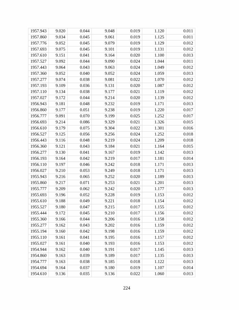
224
1957.943 9.020 0.044 9.048 0.019 1.120 0.011
1957.860 9.034 0.045 9.061 0.019 1.125 0.011
1957.776 9.052 0.045 9.079 0.019 1.129 0.012
1957.693 9.075 0.045 9.101 0.019 1.131 0.012
1957.610 9.151 0.041 9.164 0.020 1.100 0.013
1957.527 9.092 0.044 9.090 0.024 1.044 0.011
1957.443 9.064 0.043 9.063 0.024 1.049 0.012
1957.360 9.052 0.040 9.052 0.024 1.059 0.013
1957.277 9.074 0.038 9.081 0.022 1.070 0.012
1957.193 9.109 0.036 9.131 0.020 1.087 0.012
1957.110 9.134 0.038 9.177 0.021 1.119 0.012
1957.027 9.172 0.044 9.214 0.020 1.139 0.012
1956.943 9.181 0.048 9.232 0.019 1.171 0.013
1956.860 9.177 0.051 9.238 0.019 1.220 0.017
1956.777 9.091 0.070 9.199 0.025 1.252 0.017
1956.693 9.214 0.086 9.329 0.021 1.326 0.015
1956.610 9.179 0.075 9.304 0.022 1.301 0.016
1956.527 9.125 0.056 9.256 0.024 1.252 0.018
1956.443 9.116 0.048 9.219 0.024 1.209 0.018
1956.360 9.121 0.043 9.184 0.021 1.164 0.015
1956.277 9.130 0.041 9.167 0.019 1.142 0.013
1956.193 9.164 0.042 9.219 0.017 1.181 0.014
1956.110 9.197 0.046 9.242 0.018 1.171 0.013
1956.027 9.210 0.053 9.249 0.018 1.171 0.013
1955.943 9.216 0.065 9.252 0.020 1.189 0.013
1955.860 9.217 0.071 9.253 0.021 1.201 0.013
1955.777 9.209 0.062 9.242 0.020 1.177 0.013
1955.693 9.196 0.052 9.228 0.019 1.153 0.012
1955.610 9.188 0.049 9.221 0.018 1.154 0.012
1955.527 9.180 0.047 9.215 0.017 1.155 0.012
1955.444 9.172 0.045 9.210 0.017 1.156 0.012
1955.360 9.166 0.044 9.206 0.016 1.158 0.012
1955.277 9.162 0.043 9.202 0.016 1.159 0.012
1955.194 9.160 0.042 9.198 0.016 1.159 0.012
1955.110 9.161 0.041 9.195 0.016 1.157 0.012
1955.027 9.161 0.040 9.193 0.016 1.153 0.012
1954.944 9.162 0.040 9.191 0.017 1.145 0.013
1954.860 9.163 0.039 9.189 0.017 1.135 0.013
1954.777 9.163 0.038 9.185 0.018 1.122 0.013
1954.694 9.164 0.037 9.180 0.019 1.107 0.014
1954.610 9.136 0.035 9.136 0.022 1.060 0.013
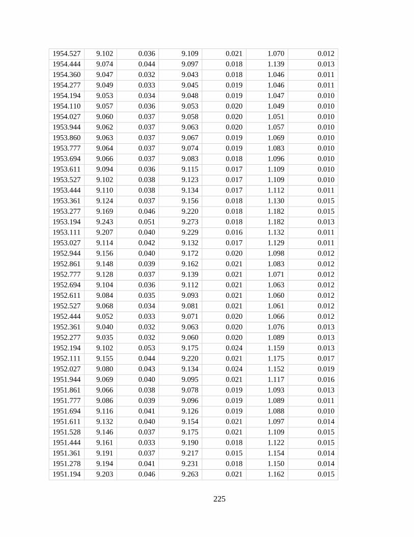
225
1954.527 9.102 0.036 9.109 0.021 1.070 0.012
1954.444 9.074 0.044 9.097 0.018 1.139 0.013
1954.360 9.047 0.032 9.043 0.018 1.046 0.011
1954.277 9.049 0.033 9.045 0.019 1.046 0.011
1954.194 9.053 0.034 9.048 0.019 1.047 0.010
1954.110 9.057 0.036 9.053 0.020 1.049 0.010
1954.027 9.060 0.037 9.058 0.020 1.051 0.010
1953.944 9.062 0.037 9.063 0.020 1.057 0.010
1953.860 9.063 0.037 9.067 0.019 1.069 0.010
1953.777 9.064 0.037 9.074 0.019 1.083 0.010
1953.694 9.066 0.037 9.083 0.018 1.096 0.010
1953.611 9.094 0.036 9.115 0.017 1.109 0.010
1953.527 9.102 0.038 9.123 0.017 1.109 0.010
1953.444 9.110 0.038 9.134 0.017 1.112 0.011
1953.361 9.124 0.037 9.156 0.018 1.130 0.015
1953.277 9.169 0.046 9.220 0.018 1.182 0.015
1953.194 9.243 0.051 9.273 0.018 1.182 0.013
1953.111 9.207 0.040 9.229 0.016 1.132 0.011
1953.027 9.114 0.042 9.132 0.017 1.129 0.011
1952.944 9.156 0.040 9.172 0.020 1.098 0.012
1952.861 9.148 0.039 9.162 0.021 1.083 0.012
1952.777 9.128 0.037 9.139 0.021 1.071 0.012
1952.694 9.104 0.036 9.112 0.021 1.063 0.012
1952.611 9.084 0.035 9.093 0.021 1.060 0.012
1952.527 9.068 0.034 9.081 0.021 1.061 0.012
1952.444 9.052 0.033 9.071 0.020 1.066 0.012
1952.361 9.040 0.032 9.063 0.020 1.076 0.013
1952.277 9.035 0.032 9.060 0.020 1.089 0.013
1952.194 9.102 0.053 9.175 0.024 1.159 0.013
1952.111 9.155 0.044 9.220 0.021 1.175 0.017
1952.027 9.080 0.043 9.134 0.024 1.152 0.019
1951.944 9.069 0.040 9.095 0.021 1.117 0.016
1951.861 9.066 0.038 9.078 0.019 1.093 0.013
1951.777 9.086 0.039 9.096 0.019 1.089 0.011
1951.694 9.116 0.041 9.126 0.019 1.088 0.010
1951.611 9.132 0.040 9.154 0.021 1.097 0.014
1951.528 9.146 0.037 9.175 0.021 1.109 0.015
1951.444 9.161 0.033 9.190 0.018 1.122 0.015
1951.361 9.191 0.037 9.217 0.015 1.154 0.014
1951.278 9.194 0.041 9.231 0.018 1.150 0.014
1951.194 9.203 0.046 9.263 0.021 1.162 0.015
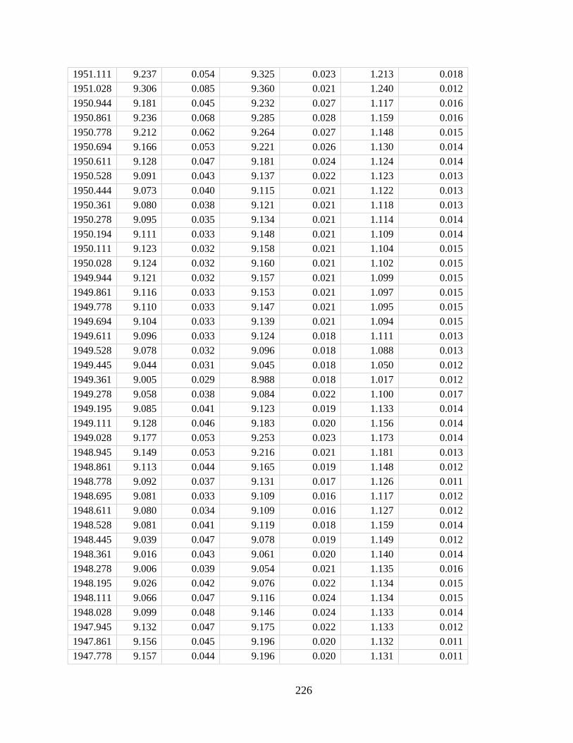
226
1951.111 9.237 0.054 9.325 0.023 1.213 0.018
1951.028 9.306 0.085 9.360 0.021 1.240 0.012
1950.944 9.181 0.045 9.232 0.027 1.117 0.016
1950.861 9.236 0.068 9.285 0.028 1.159 0.016
1950.778 9.212 0.062 9.264 0.027 1.148 0.015
1950.694 9.166 0.053 9.221 0.026 1.130 0.014
1950.611 9.128 0.047 9.181 0.024 1.124 0.014
1950.528 9.091 0.043 9.137 0.022 1.123 0.013
1950.444 9.073 0.040 9.115 0.021 1.122 0.013
1950.361 9.080 0.038 9.121 0.021 1.118 0.013
1950.278 9.095 0.035 9.134 0.021 1.114 0.014
1950.194 9.111 0.033 9.148 0.021 1.109 0.014
1950.111 9.123 0.032 9.158 0.021 1.104 0.015
1950.028 9.124 0.032 9.160 0.021 1.102 0.015
1949.944 9.121 0.032 9.157 0.021 1.099 0.015
1949.861 9.116 0.033 9.153 0.021 1.097 0.015
1949.778 9.110 0.033 9.147 0.021 1.095 0.015
1949.694 9.104 0.033 9.139 0.021 1.094 0.015
1949.611 9.096 0.033 9.124 0.018 1.111 0.013
1949.528 9.078 0.032 9.096 0.018 1.088 0.013
1949.445 9.044 0.031 9.045 0.018 1.050 0.012
1949.361 9.005 0.029 8.988 0.018 1.017 0.012
1949.278 9.058 0.038 9.084 0.022 1.100 0.017
1949.195 9.085 0.041 9.123 0.019 1.133 0.014
1949.111 9.128 0.046 9.183 0.020 1.156 0.014
1949.028 9.177 0.053 9.253 0.023 1.173 0.014
1948.945 9.149 0.053 9.216 0.021 1.181 0.013
1948.861 9.113 0.044 9.165 0.019 1.148 0.012
1948.778 9.092 0.037 9.131 0.017 1.126 0.011
1948.695 9.081 0.033 9.109 0.016 1.117 0.012
1948.611 9.080 0.034 9.109 0.016 1.127 0.012
1948.528 9.081 0.041 9.119 0.018 1.159 0.014
1948.445 9.039 0.047 9.078 0.019 1.149 0.012
1948.361 9.016 0.043 9.061 0.020 1.140 0.014
1948.278 9.006 0.039 9.054 0.021 1.135 0.016
1948.195 9.026 0.042 9.076 0.022 1.134 0.015
1948.111 9.066 0.047 9.116 0.024 1.134 0.015
1948.028 9.099 0.048 9.146 0.024 1.133 0.014
1947.945 9.132 0.047 9.175 0.022 1.133 0.012
1947.861 9.156 0.045 9.196 0.020 1.132 0.011
1947.778 9.157 0.044 9.196 0.020 1.131 0.011
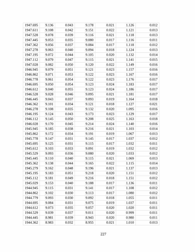
227
1947.695 9.136 0.043 9.178 0.021 1.126 0.012
1947.611 9.108 0.042 9.151 0.022 1.121 0.013
1947.528 9.078 0.039 9.116 0.021 1.118 0.013
1947.445 9.053 0.035 9.080 0.017 1.116 0.011
1947.362 9.056 0.037 9.084 0.017 1.118 0.012
1947.278 9.063 0.040 9.094 0.018 1.124 0.013
1947.195 9.072 0.044 9.105 0.020 1.132 0.014
1947.112 9.079 0.047 9.115 0.021 1.141 0.015
1947.028 9.082 0.050 9.120 0.022 1.149 0.016
1946.945 9.079 0.051 9.121 0.023 1.157 0.016
1946.862 9.071 0.053 9.122 0.023 1.167 0.016
1946.778 9.061 0.054 9.122 0.023 1.176 0.017
1946.695 9.050 0.054 9.123 0.024 1.183 0.017
1946.612 9.040 0.055 9.123 0.024 1.186 0.017
1946.528 9.028 0.046 9.095 0.021 1.181 0.017
1946.445 9.043 0.037 9.093 0.019 1.164 0.018
1946.362 9.101 0.034 9.121 0.018 1.127 0.021
1946.278 9.108 0.035 9.132 0.020 1.095 0.016
1946.195 9.124 0.043 9.173 0.023 1.129 0.017
1946.112 9.145 0.050 9.208 0.025 1.163 0.018
1946.028 9.170 0.045 9.214 0.024 1.140 0.016
1945.945 9.185 0.038 9.216 0.021 1.103 0.014
1945.862 9.172 0.034 9.191 0.019 1.067 0.013
1945.778 9.147 0.031 9.145 0.017 1.037 0.012
1945.695 9.125 0.031 9.115 0.017 1.032 0.011
1945.612 9.103 0.033 9.091 0.019 1.032 0.012
1945.529 9.093 0.036 9.080 0.020 1.033 0.012
1945.445 9.110 0.040 9.115 0.021 1.069 0.013
1945.362 9.138 0.044 9.165 0.022 1.115 0.014
1945.279 9.162 0.048 9.196 0.021 1.137 0.013
1945.195 9.183 0.051 9.218 0.020 1.151 0.012
1945.112 9.181 0.049 9.216 0.018 1.151 0.012
1945.029 9.153 0.040 9.188 0.017 1.136 0.011
1944.945 9.115 0.031 9.141 0.017 1.108 0.012
1944.862 9.102 0.030 9.113 0.017 1.080 0.012
1944.779 9.093 0.030 9.092 0.018 1.055 0.011
1944.695 9.084 0.031 9.075 0.019 1.037 0.011
1944.612 9.073 0.035 9.057 0.020 1.020 0.011
1944.529 9.039 0.037 9.011 0.020 0.999 0.011
1944.445 8.981 0.039 8.943 0.020 0.980 0.011
1944.362 8.983 0.032 8.955 0.021 1.010 0.013
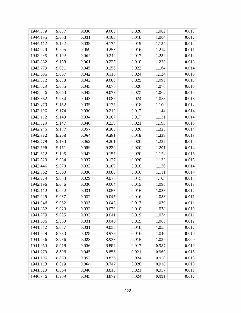
228
1944.279 9.057 0.030 9.068 0.020 1.062 0.012
1944.195 9.088 0.031 9.103 0.018 1.084 0.012
1944.112 9.132 0.039 9.175 0.019 1.135 0.012
1944.029 9.205 0.059 9.253 0.016 1.214 0.011
1943.945 9.192 0.064 9.249 0.017 1.232 0.012
1943.862 9.158 0.061 9.227 0.018 1.223 0.013
1943.779 9.091 0.045 9.158 0.022 1.164 0.014
1943.695 9.067 0.042 9.116 0.024 1.124 0.015
1943.612 9.058 0.043 9.088 0.025 1.098 0.013
1943.529 9.055 0.043 9.076 0.026 1.078 0.013
1943.446 9.063 0.043 9.079 0.025 1.062 0.013
1943.362 9.084 0.043 9.086 0.024 1.053 0.013
1943.279 9.152 0.035 9.177 0.018 1.109 0.012
1943.196 9.174 0.036 9.212 0.017 1.144 0.014
1943.112 9.149 0.034 9.187 0.017 1.131 0.014
1943.029 9.147 0.046 9.239 0.021 1.193 0.015
1942.946 9.177 0.057 9.268 0.020 1.225 0.014
1942.862 9.208 0.064 9.281 0.019 1.239 0.013
1942.779 9.193 0.062 9.261 0.020 1.227 0.014
1942.696 9.161 0.059 9.220 0.020 1.201 0.014
1942.612 9.105 0.043 9.157 0.020 1.152 0.015
1942.529 9.084 0.037 9.127 0.020 1.133 0.015
1942.446 9.070 0.033 9.105 0.018 1.120 0.014
1942.362 9.060 0.030 9.089 0.016 1.111 0.014
1942.279 9.053 0.029 9.076 0.015 1.103 0.013
1942.196 9.046 0.030 9.064 0.015 1.095 0.013
1942.112 9.042 0.031 9.055 0.016 1.088 0.012
1942.029 9.037 0.032 9.047 0.016 1.083 0.011
1941.946 9.032 0.033 9.042 0.017 1.079 0.011
1941.862 9.023 0.033 9.039 0.018 1.078 0.010
1941.779 9.025 0.033 9.041 0.019 1.074 0.011
1941.696 9.039 0.031 9.046 0.019 1.065 0.012
1941.612 9.037 0.031 9.033 0.018 1.053 0.012
1941.529 8.980 0.028 8.978 0.016 1.046 0.010
1941.446 8.936 0.028 8.938 0.015 1.034 0.009
1941.363 8.918 0.036 8.884 0.017 0.987 0.010
1941.279 8.896 0.045 8.856 0.021 0.969 0.013
1941.196 8.883 0.052 8.836 0.024 0.958 0.013
1941.113 8.819 0.064 8.747 0.020 0.916 0.010
1941.029 8.864 0.048 8.813 0.021 0.957 0.011
1940.946 8.909 0.045 8.872 0.024 0.991 0.012
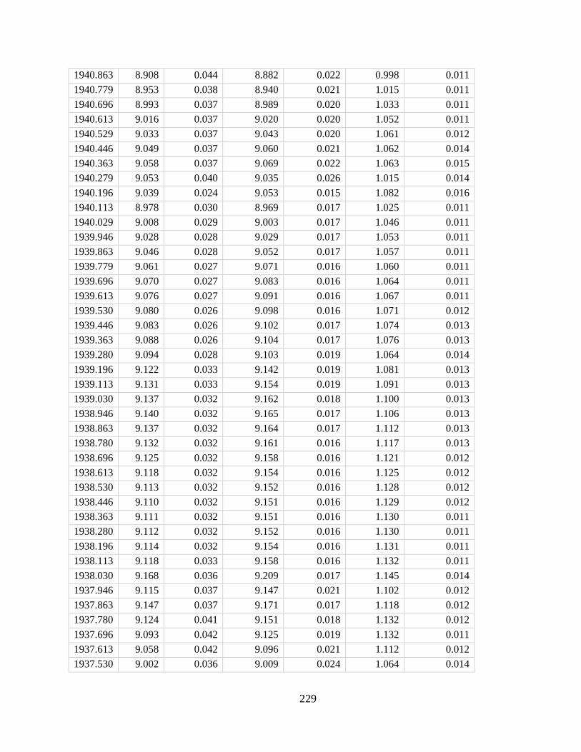
229
1940.863 8.908 0.044 8.882 0.022 0.998 0.011
1940.779 8.953 0.038 8.940 0.021 1.015 0.011
1940.696 8.993 0.037 8.989 0.020 1.033 0.011
1940.613 9.016 0.037 9.020 0.020 1.052 0.011
1940.529 9.033 0.037 9.043 0.020 1.061 0.012
1940.446 9.049 0.037 9.060 0.021 1.062 0.014
1940.363 9.058 0.037 9.069 0.022 1.063 0.015
1940.279 9.053 0.040 9.035 0.026 1.015 0.014
1940.196 9.039 0.024 9.053 0.015 1.082 0.016
1940.113 8.978 0.030 8.969 0.017 1.025 0.011
1940.029 9.008 0.029 9.003 0.017 1.046 0.011
1939.946 9.028 0.028 9.029 0.017 1.053 0.011
1939.863 9.046 0.028 9.052 0.017 1.057 0.011
1939.779 9.061 0.027 9.071 0.016 1.060 0.011
1939.696 9.070 0.027 9.083 0.016 1.064 0.011
1939.613 9.076 0.027 9.091 0.016 1.067 0.011
1939.530 9.080 0.026 9.098 0.016 1.071 0.012
1939.446 9.083 0.026 9.102 0.017 1.074 0.013
1939.363 9.088 0.026 9.104 0.017 1.076 0.013
1939.280 9.094 0.028 9.103 0.019 1.064 0.014
1939.196 9.122 0.033 9.142 0.019 1.081 0.013
1939.113 9.131 0.033 9.154 0.019 1.091 0.013
1939.030 9.137 0.032 9.162 0.018 1.100 0.013
1938.946 9.140 0.032 9.165 0.017 1.106 0.013
1938.863 9.137 0.032 9.164 0.017 1.112 0.013
1938.780 9.132 0.032 9.161 0.016 1.117 0.013
1938.696 9.125 0.032 9.158 0.016 1.121 0.012
1938.613 9.118 0.032 9.154 0.016 1.125 0.012
1938.530 9.113 0.032 9.152 0.016 1.128 0.012
1938.446 9.110 0.032 9.151 0.016 1.129 0.012
1938.363 9.111 0.032 9.151 0.016 1.130 0.011
1938.280 9.112 0.032 9.152 0.016 1.130 0.011
1938.196 9.114 0.032 9.154 0.016 1.131 0.011
1938.113 9.118 0.033 9.158 0.016 1.132 0.011
1938.030 9.168 0.036 9.209 0.017 1.145 0.014
1937.946 9.115 0.037 9.147 0.021 1.102 0.012
1937.863 9.147 0.037 9.171 0.017 1.118 0.012
1937.780 9.124 0.041 9.151 0.018 1.132 0.012
1937.696 9.093 0.042 9.125 0.019 1.132 0.011
1937.613 9.058 0.042 9.096 0.021 1.112 0.012
1937.530 9.002 0.036 9.009 0.024 1.064 0.014
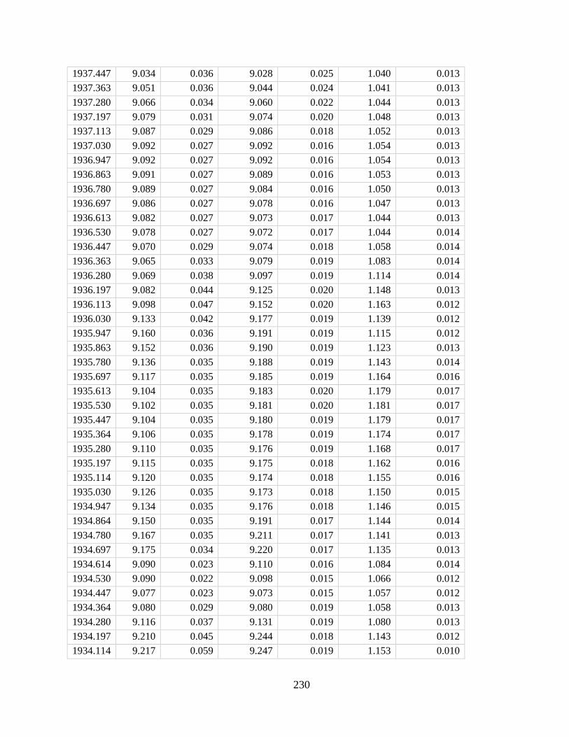
230
1937.447 9.034 0.036 9.028 0.025 1.040 0.013
1937.363 9.051 0.036 9.044 0.024 1.041 0.013
1937.280 9.066 0.034 9.060 0.022 1.044 0.013
1937.197 9.079 0.031 9.074 0.020 1.048 0.013
1937.113 9.087 0.029 9.086 0.018 1.052 0.013
1937.030 9.092 0.027 9.092 0.016 1.054 0.013
1936.947 9.092 0.027 9.092 0.016 1.054 0.013
1936.863 9.091 0.027 9.089 0.016 1.053 0.013
1936.780 9.089 0.027 9.084 0.016 1.050 0.013
1936.697 9.086 0.027 9.078 0.016 1.047 0.013
1936.613 9.082 0.027 9.073 0.017 1.044 0.013
1936.530 9.078 0.027 9.072 0.017 1.044 0.014
1936.447 9.070 0.029 9.074 0.018 1.058 0.014
1936.363 9.065 0.033 9.079 0.019 1.083 0.014
1936.280 9.069 0.038 9.097 0.019 1.114 0.014
1936.197 9.082 0.044 9.125 0.020 1.148 0.013
1936.113 9.098 0.047 9.152 0.020 1.163 0.012
1936.030 9.133 0.042 9.177 0.019 1.139 0.012
1935.947 9.160 0.036 9.191 0.019 1.115 0.012
1935.863 9.152 0.036 9.190 0.019 1.123 0.013
1935.780 9.136 0.035 9.188 0.019 1.143 0.014
1935.697 9.117 0.035 9.185 0.019 1.164 0.016
1935.613 9.104 0.035 9.183 0.020 1.179 0.017
1935.530 9.102 0.035 9.181 0.020 1.181 0.017
1935.447 9.104 0.035 9.180 0.019 1.179 0.017
1935.364 9.106 0.035 9.178 0.019 1.174 0.017
1935.280 9.110 0.035 9.176 0.019 1.168 0.017
1935.197 9.115 0.035 9.175 0.018 1.162 0.016
1935.114 9.120 0.035 9.174 0.018 1.155 0.016
1935.030 9.126 0.035 9.173 0.018 1.150 0.015
1934.947 9.134 0.035 9.176 0.018 1.146 0.015
1934.864 9.150 0.035 9.191 0.017 1.144 0.014
1934.780 9.167 0.035 9.211 0.017 1.141 0.013
1934.697 9.175 0.034 9.220 0.017 1.135 0.013
1934.614 9.090 0.023 9.110 0.016 1.084 0.014
1934.530 9.090 0.022 9.098 0.015 1.066 0.012
1934.447 9.077 0.023 9.073 0.015 1.057 0.012
1934.364 9.080 0.029 9.080 0.019 1.058 0.013
1934.280 9.116 0.037 9.131 0.019 1.080 0.013
1934.197 9.210 0.045 9.244 0.018 1.143 0.012
1934.114 9.217 0.059 9.247 0.019 1.153 0.010
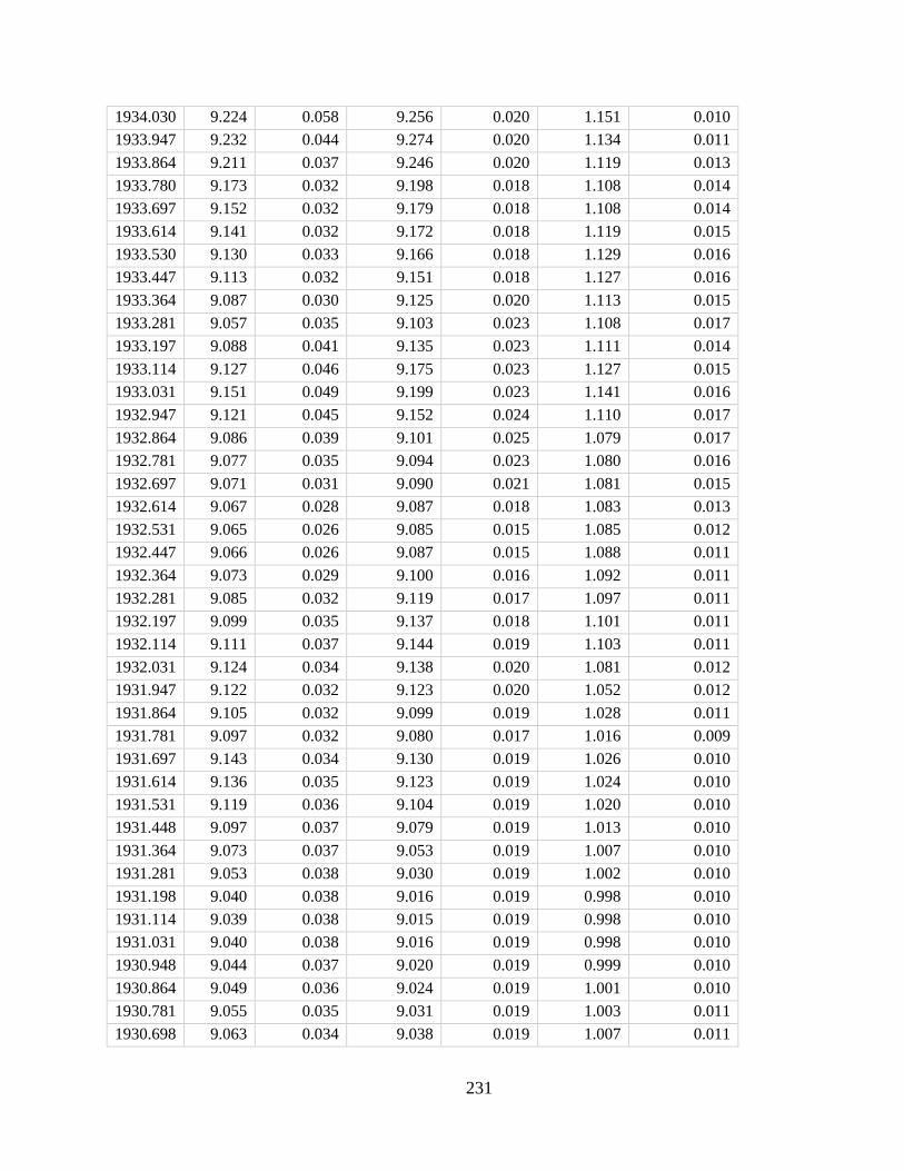
231
1934.030 9.224 0.058 9.256 0.020 1.151 0.010
1933.947 9.232 0.044 9.274 0.020 1.134 0.011
1933.864 9.211 0.037 9.246 0.020 1.119 0.013
1933.780 9.173 0.032 9.198 0.018 1.108 0.014
1933.697 9.152 0.032 9.179 0.018 1.108 0.014
1933.614 9.141 0.032 9.172 0.018 1.119 0.015
1933.530 9.130 0.033 9.166 0.018 1.129 0.016
1933.447 9.113 0.032 9.151 0.018 1.127 0.016
1933.364 9.087 0.030 9.125 0.020 1.113 0.015
1933.281 9.057 0.035 9.103 0.023 1.108 0.017
1933.197 9.088 0.041 9.135 0.023 1.111 0.014
1933.114 9.127 0.046 9.175 0.023 1.127 0.015
1933.031 9.151 0.049 9.199 0.023 1.141 0.016
1932.947 9.121 0.045 9.152 0.024 1.110 0.017
1932.864 9.086 0.039 9.101 0.025 1.079 0.017
1932.781 9.077 0.035 9.094 0.023 1.080 0.016
1932.697 9.071 0.031 9.090 0.021 1.081 0.015
1932.614 9.067 0.028 9.087 0.018 1.083 0.013
1932.531 9.065 0.026 9.085 0.015 1.085 0.012
1932.447 9.066 0.026 9.087 0.015 1.088 0.011
1932.364 9.073 0.029 9.100 0.016 1.092 0.011
1932.281 9.085 0.032 9.119 0.017 1.097 0.011
1932.197 9.099 0.035 9.137 0.018 1.101 0.011
1932.114 9.111 0.037 9.144 0.019 1.103 0.011
1932.031 9.124 0.034 9.138 0.020 1.081 0.012
1931.947 9.122 0.032 9.123 0.020 1.052 0.012
1931.864 9.105 0.032 9.099 0.019 1.028 0.011
1931.781 9.097 0.032 9.080 0.017 1.016 0.009
1931.697 9.143 0.034 9.130 0.019 1.026 0.010
1931.614 9.136 0.035 9.123 0.019 1.024 0.010
1931.531 9.119 0.036 9.104 0.019 1.020 0.010
1931.448 9.097 0.037 9.079 0.019 1.013 0.010
1931.364 9.073 0.037 9.053 0.019 1.007 0.010
1931.281 9.053 0.038 9.030 0.019 1.002 0.010
1931.198 9.040 0.038 9.016 0.019 0.998 0.010
1931.114 9.039 0.038 9.015 0.019 0.998 0.010
1931.031 9.040 0.038 9.016 0.019 0.998 0.010
1930.948 9.044 0.037 9.020 0.019 0.999 0.010
1930.864 9.049 0.036 9.024 0.019 1.001 0.010
1930.781 9.055 0.035 9.031 0.019 1.003 0.011
1930.698 9.063 0.034 9.038 0.019 1.007 0.011
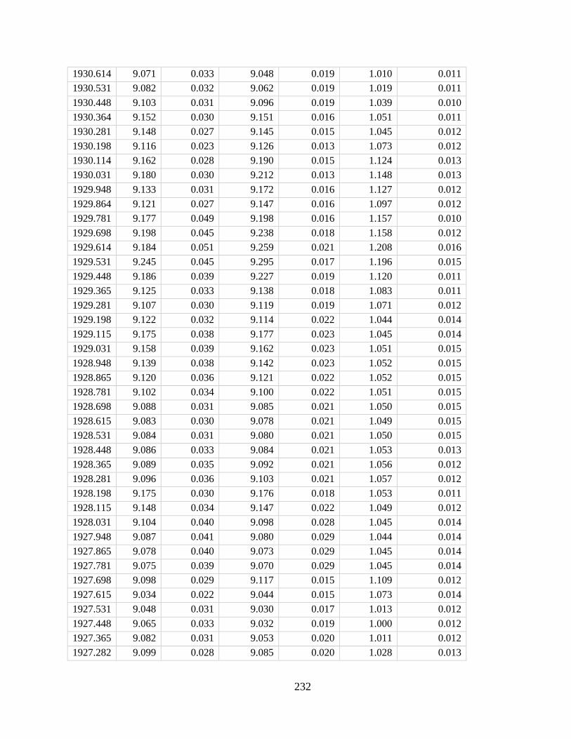
232
1930.614 9.071 0.033 9.048 0.019 1.010 0.011
1930.531 9.082 0.032 9.062 0.019 1.019 0.011
1930.448 9.103 0.031 9.096 0.019 1.039 0.010
1930.364 9.152 0.030 9.151 0.016 1.051 0.011
1930.281 9.148 0.027 9.145 0.015 1.045 0.012
1930.198 9.116 0.023 9.126 0.013 1.073 0.012
1930.114 9.162 0.028 9.190 0.015 1.124 0.013
1930.031 9.180 0.030 9.212 0.013 1.148 0.013
1929.948 9.133 0.031 9.172 0.016 1.127 0.012
1929.864 9.121 0.027 9.147 0.016 1.097 0.012
1929.781 9.177 0.049 9.198 0.016 1.157 0.010
1929.698 9.198 0.045 9.238 0.018 1.158 0.012
1929.614 9.184 0.051 9.259 0.021 1.208 0.016
1929.531 9.245 0.045 9.295 0.017 1.196 0.015
1929.448 9.186 0.039 9.227 0.019 1.120 0.011
1929.365 9.125 0.033 9.138 0.018 1.083 0.011
1929.281 9.107 0.030 9.119 0.019 1.071 0.012
1929.198 9.122 0.032 9.114 0.022 1.044 0.014
1929.115 9.175 0.038 9.177 0.023 1.045 0.014
1929.031 9.158 0.039 9.162 0.023 1.051 0.015
1928.948 9.139 0.038 9.142 0.023 1.052 0.015
1928.865 9.120 0.036 9.121 0.022 1.052 0.015
1928.781 9.102 0.034 9.100 0.022 1.051 0.015
1928.698 9.088 0.031 9.085 0.021 1.050 0.015
1928.615 9.083 0.030 9.078 0.021 1.049 0.015
1928.531 9.084 0.031 9.080 0.021 1.050 0.015
1928.448 9.086 0.033 9.084 0.021 1.053 0.013
1928.365 9.089 0.035 9.092 0.021 1.056 0.012
1928.281 9.096 0.036 9.103 0.021 1.057 0.012
1928.198 9.175 0.030 9.176 0.018 1.053 0.011
1928.115 9.148 0.034 9.147 0.022 1.049 0.012
1928.031 9.104 0.040 9.098 0.028 1.045 0.014
1927.948 9.087 0.041 9.080 0.029 1.044 0.014
1927.865 9.078 0.040 9.073 0.029 1.045 0.014
1927.781 9.075 0.039 9.070 0.029 1.045 0.014
1927.698 9.098 0.029 9.117 0.015 1.109 0.012
1927.615 9.034 0.022 9.044 0.015 1.073 0.014
1927.531 9.048 0.031 9.030 0.017 1.013 0.012
1927.448 9.065 0.033 9.032 0.019 1.000 0.012
1927.365 9.082 0.031 9.053 0.020 1.011 0.012
1927.282 9.099 0.028 9.085 0.020 1.028 0.013
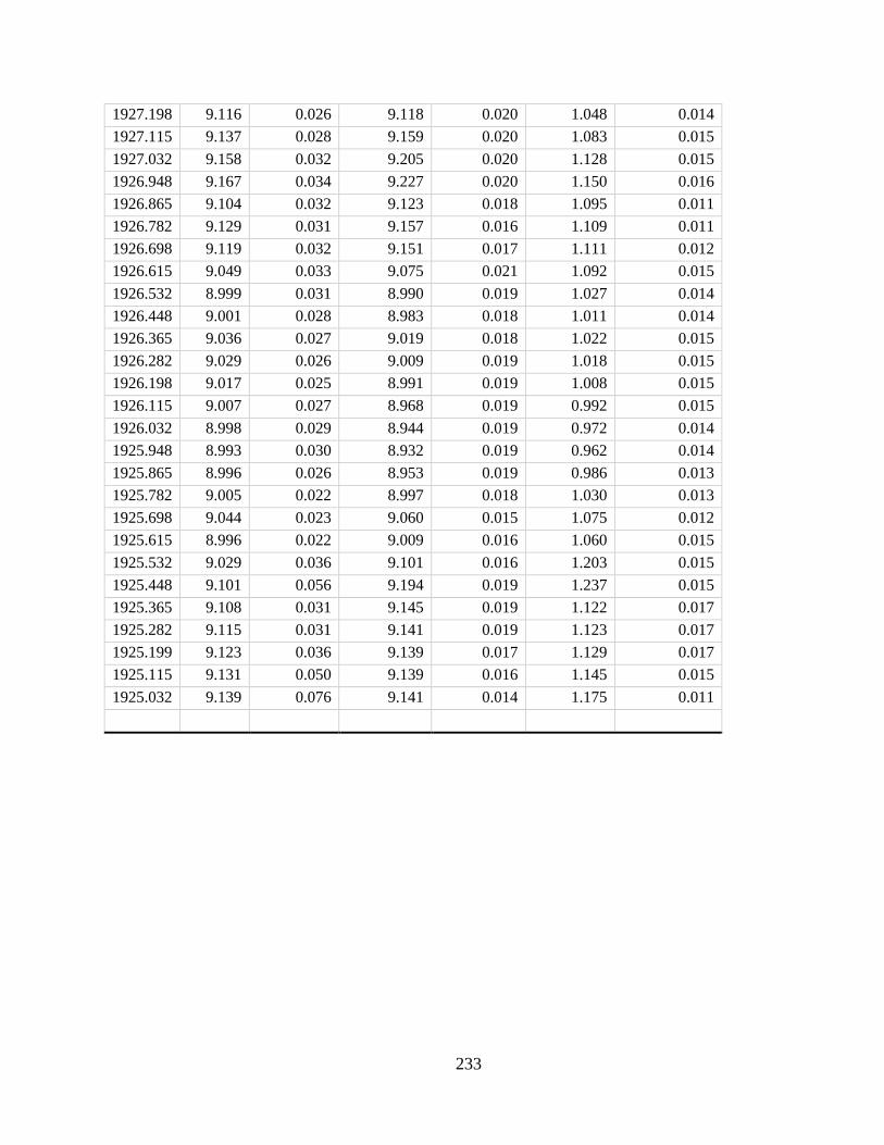
233
1927.198 9.116 0.026 9.118 0.020 1.048 0.014
1927.115 9.137 0.028 9.159 0.020 1.083 0.015
1927.032 9.158 0.032 9.205 0.020 1.128 0.015
1926.948 9.167 0.034 9.227 0.020 1.150 0.016
1926.865 9.104 0.032 9.123 0.018 1.095 0.011
1926.782 9.129 0.031 9.157 0.016 1.109 0.011
1926.698 9.119 0.032 9.151 0.017 1.111 0.012
1926.615 9.049 0.033 9.075 0.021 1.092 0.015
1926.532 8.999 0.031 8.990 0.019 1.027 0.014
1926.448 9.001 0.028 8.983 0.018 1.011 0.014
1926.365 9.036 0.027 9.019 0.018 1.022 0.015
1926.282 9.029 0.026 9.009 0.019 1.018 0.015
1926.198 9.017 0.025 8.991 0.019 1.008 0.015
1926.115 9.007 0.027 8.968 0.019 0.992 0.015
1926.032 8.998 0.029 8.944 0.019 0.972 0.014
1925.948 8.993 0.030 8.932 0.019 0.962 0.014
1925.865 8.996 0.026 8.953 0.019 0.986 0.013
1925.782 9.005 0.022 8.997 0.018 1.030 0.013
1925.698 9.044 0.023 9.060 0.015 1.075 0.012
1925.615 8.996 0.022 9.009 0.016 1.060 0.015
1925.532 9.029 0.036 9.101 0.016 1.203 0.015
1925.448 9.101 0.056 9.194 0.019 1.237 0.015
1925.365 9.108 0.031 9.145 0.019 1.122 0.017
1925.282 9.115 0.031 9.141 0.019 1.123 0.017
1925.199 9.123 0.036 9.139 0.017 1.129 0.017
1925.115 9.131 0.050 9.139 0.016 1.145 0.015
1925.032 9.139 0.076 9.141 0.014 1.175 0.011
234
A5.2 References
Cheng H, Edwards RL, Shen C, Polyak VJ, Asmerom Y, Woodhead J, Hellstrom J, Wang Y, Kong
X, Spötl C, Wang X, Alexander EC (2013) Improvements in 230Th dating , 230Th and 234U
half-life values , and U – Th isotopic measurements by multi-collector inductively coupled
plasma mass spectrometry. Earth Planet Sci Lett 371–372:82–91
Jaffey AH, Flynn KF, Glendenin LE, Bentley WC, Essling AM (1971) Precision Measurement of
Half-Lives and Specific Activities of 235U and 238U. Phys Rev C 4: