Copyright

by

David Andrew Holmes McCleary

2012

The Thesis Committee for David Andrew Holmes McCleary

Certifies that this is the approved version of the following thesis:

Three Dimensional Computational Modeling of Electrochemical

Performance and Heat Generation in Spirally and Prismatically Wound

Configurations

APPROVED BY

SUPERVISING COMMITTEE:

Jeremy Meyers

Ofodike Ezekoye

Supervisor:

Three Dimensional Computational Modeling of Electrochemical

Performance and Heat Generation in Spirally and Prismatically Wound

Configurations

by

David Andrew Holmes McCleary, B.S.M.E.

Thesis

Presented to the Faculty of the Graduate School of

The University of Texas at Austin

in Partial Fulfillment

of the Requirements

for the Degree of

Master of Science in Engineering

The University of Texas at Austin

August 2012

iv

Acknowledgements

I would first like to thank my advisor, Dr. Jeremy Meyers, for the opportunity to

work on this project. I learned a great deal about electrochemistry and batteries in

particular, which was my reason for attending UT.

I would also like to thank Dr. Beomkeun Kim, a visiting professor from South

Korea, for providing supplemental guidance over the past eight months. His

understanding of modeling helped “connect the dots” between electrochemical and

thermal concepts, which saved a great deal of time. Also his experienced approach

towards this research helped me produce a thesis that I am proud of.

Lastly, I would like to thank A123 Systems for the opportunity to explore their

technology. Also thank you to the University of Texas at Austin College of Engineering,

the Booker family, and George J. Heuer, Jr. for the fellowships that provided funding to

enable me to accomplish my goals.

v

Abstract

Three Dimensional Computational Modeling of Electrochemical

Performance and Heat Generation in Spirally and Prismatically Wound

Configurations

David Andrew Holmes McCleary, M.S.E.

The University of Texas at Austin, 2012

Supervisor: Jeremy Meyers

This thesis details a three dimensional model for simulating the operation of two

particular configurations of a lithium iron phosphate (LiFePO4) battery. Large-scale

lithium iron phosphate batteries are becoming increasingly important in a world that

demands portable energy that is high in both power and energy density, particularly for

hybrid and electric vehicles. Understanding how batteries of this type operate is

important for the design, optimization, and control of their performance, safety and

durability. While 1D approximations may be sufficient for small scale or single cell

batteries, these approximations are limited when scaled up to larger batteries, where

significant three dimensional gradients might develop including lithium ion

concentration, temperature, current density and voltage gradients. This model is able to

account for all of these gradients in three dimensions by coupling an electrochemical

model with a thermal model. This coupling shows how electrochemical performance

affects temperature distribution and to a lesser extent how temperature affects

electrochemical performance. This model is applicable to two battery configurations —

spirally wound and prismatically wound. Results generated include temperature

influences on current distribution and vice versa, an exploration of various cooling

environments’ effects on performance, design optimization of current collector thickness

and current collector tab placement, and an analysis of lithium plating risk.

vi

Table of Contents

CHAPTER 1: BACKGROUND .....................................................................................1

1.1 Introduction ........................................................................................................1

1.2 Battery Structure ................................................................................................2

1.2.1 Single Electrochemical Cell ...................................................................2

1.2.2 Electrochemical Cells within a Real Battery .........................................3

1.2.3 Spirally Wound and Prismatically Wound Batteries .............................4

1.2.4 Specific Materials ..................................................................................6

1.3 Prior 3D Modeling of Batteries ..........................................................................6

CHAPTER 2:MATHEMATICAL MODEL OF WOUND BATTERY

CONFIGURATIONS..................................................................................................10

2.1 Modeling the Battery as a 3D Network of Resistors .......................................10

2.1.1 Current Collector and Electrochemical Reaction Resistors .................10

2.1.2 Alignment of Nodes in Wound Configurations ...................................14

2.1.3 Archimedes' Spiral Theory and Application ........................................15

2.1.4 Prismatically Wound Battery as Concentric Layers ............................19

2.2 Models..............................................................................................................19

2.2.1 Electrochemical Model ........................................................................20

2.2.2 Thermal Model and Coupling with Electrochemical Model ...............21

2.3 Numerical Methods ..........................................................................................22

2.3.1 Finite Difference Method .....................................................................22

2.3.2 Solution Phase Concentration Control Volume Method .....................23

2.3.3 Solid Phase Duhamel's Superposition Integral ....................................24

2.3.4 Newton Raphson Method ....................................................................24

vii

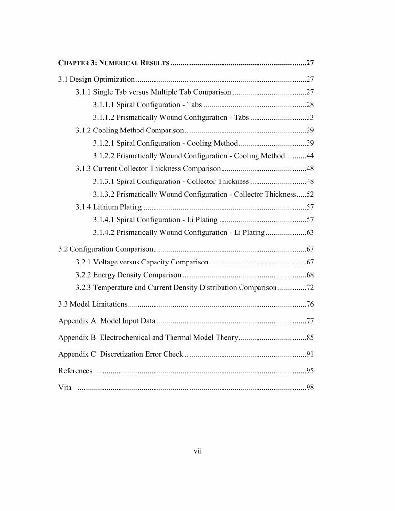
CHAPTER 3: NUMERICAL RESULTS ......................................................................27

3.1 Design Optimization ........................................................................................27

3.1.1 Single Tab versus Multiple Tab Comparison ......................................27

3.1.1.1 Spiral Configuration - Tabs .....................................................28

3.1.1.2 Prismatically Wound Configuration - Tabs .............................33

3.1.2 Cooling Method Comparison ...............................................................39

3.1.2.1 Spiral Configuration - Cooling Method ...................................39

3.1.2.2 Prismatically Wound Configuration - Cooling Method...........44

3.1.3 Current Collector Thickness Comparison ............................................48

3.1.3.1 Spiral Configuration - Collector Thickness .............................48

3.1.3.2 Prismatically Wound Configuration - Collector Thickness .....52

3.1.4 Lithium Plating ....................................................................................57

3.1.4.1 Spiral Configuration - Li Plating .............................................57

3.1.4.2 Prismatically Wound Configuration - Li Plating .....................63

3.2 Configuration Comparison...............................................................................67

3.2.1 Voltage versus Capacity Comparison ..................................................67

3.2.2 Energy Density Comparison ................................................................68

3.2.3 Temperature and Current Density Distribution Comparison ...............72

3.3 Model Limitations ............................................................................................76

Appendix A Model Input Data .............................................................................77

Appendix B Electrochemical and Thermal Model Theory ...................................85

Appendix C Discretization Error Check ...............................................................91

References ..............................................................................................................95

Vita ......................................................................................................................98

1

CHAPTER 1: BACKGROUND

1.1 Introduction

Over the past two decades lithium ion batteries have revolutionized the tech

industry. Through high power and energy densities, lithium ion batteries have become the

primary battery chemistry for cellular phones and portable laptops. As the auto industry

evolves it will rely more heavily upon batteries for hybrid and pure electric applications.

Lithium ion batteries are a likely candidate to change how vehicles are powered.

Unlike small-scale batteries for personal devices, which only need to last for a

few years, large-scale lithium ion batteries for vehicles will ultimately need to last for the

life of the car, around 100,000 miles or 10 years. Therefore, durability, performance and

safety are critical characteristics of the batteries placed in these vehicles. Temperature

and risk of lithium plating are related directly to safety, while design factors such as

current extraction tab locations and current collector thickness are key to performance; all

are coupled to one another and affect durability.

Several factors are explored in this study. Non-uniform temperature across a

battery cell can cause the materials to break down quicker and potentially lead to thermal

runaway. Whenever the potential of the electrolyte exceeds that of the adjacent negative

electrode during a charging event, there is potential for lithium to plate out onto the

electrode. Once this occurs it is probable that dendrites will form, and unless the plating

is stopped they will grow and pierce the membrane to cause a short circuit, permanently

damaging the cell. Tab size and location dictates current flow through a cell and can

cause non-uniformities of current density and consequently temperature. As current

collector thickness is increased, it will improve current density uniformity but sacrifice

specific energy density. Side reactions may also occur in the battery when in a highly

charged state. All of these factors must be considered to reach the objectives of large

scale lithium ion batteries.

In this thesis various design parameters and operating procedures are explored for

two different configurations of a lithium iron phosphate battery. For two configurations,

temperature, current density and gradients, as well as ionic concentration across the cell

2

will be monitored and analyzed. For this thesis, a computational model that predicts the

performance of the battery in three dimensions was developed. The model is used to

make recommendations for design optimization and operation.

1.2 Battery Structure

Electrochemical energy storage devices are commonly referred to as batteries.

These devices store energy chemically. When connected to an external circuit the

chemical energy is converted into useful electrical energy. To accomplish this, the battery

must have five different layers: the negative current collector, negative electrode,

separator, positive electrode, and positive current collector.

1.2.1 SINGLE ELECTROCHEMICAL CELL

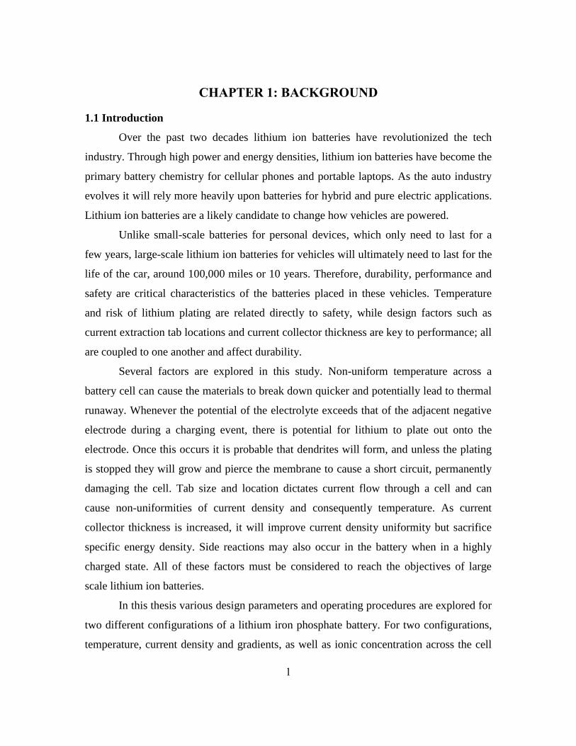
In a single electrochemical cell, lithium ions (Li+) are shuttled from one electrode

to the other through the separator; the direction the ions flow depends on whether the

battery is charging or discharging. No matter which direction a lithium ion travels, when

it leaves one electrode the electron that was paired with it travels through an external

circuit and meets up with the lithium ion on the other electrode. When attempting to draw

electricity from a battery, the negative electrode is called the anode and the positive

electrode is the cathode. See Figure 1 for a basic diagram of a battery being discharged.

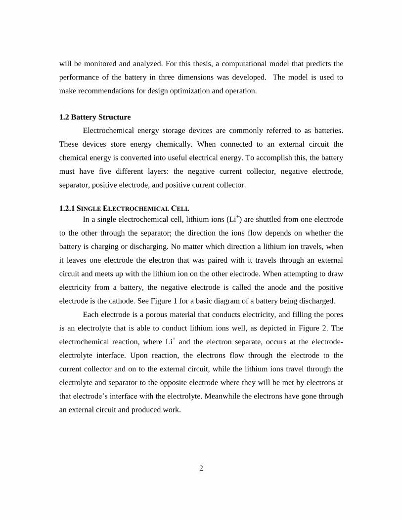
Each electrode is a porous material that conducts electricity, and filling the pores

is an electrolyte that is able to conduct lithium ions well, as depicted in Figure 2. The

electrochemical reaction, where Li+ and the electron separate, occurs at the electrode-

electrolyte interface. Upon reaction, the electrons flow through the electrode to the

current collector and on to the external circuit, while the lithium ions travel through the

electrolyte and separator to the opposite electrode where they will be met by electrons at

that electrode’s interface with the electrolyte. Meanwhile the electrons have gone through

an external circuit and produced work.

3

Figure 1: Diagram of a lithium-ion battery being discharged.

Figure 2: Representation of a porous electrode under microscope. The electrochemical

reaction occurs at the electrolyte – electrode interface.

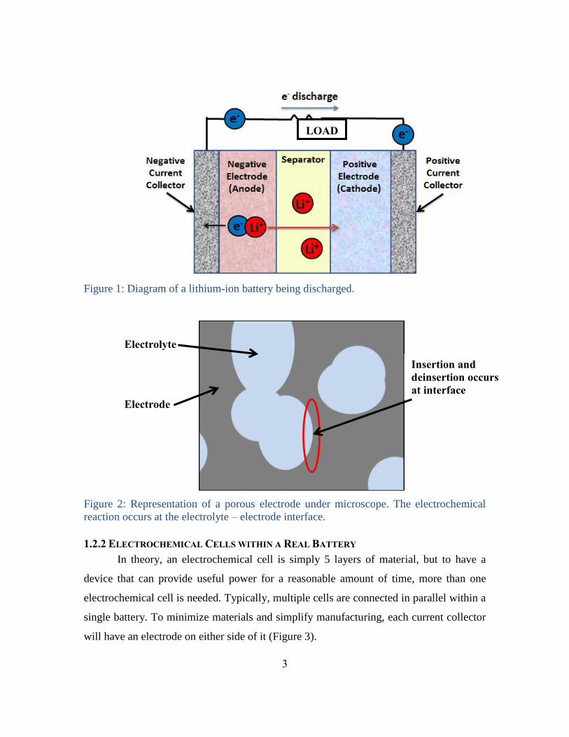
1.2.2 ELECTROCHEMICAL CELLS WITHIN A REAL BATTERY

In theory, an electrochemical cell is simply 5 layers of material, but to have a

device that can provide useful power for a reasonable amount of time, more than one

electrochemical cell is needed. Typically, multiple cells are connected in parallel within a

single battery. To minimize materials and simplify manufacturing, each current collector

will have an electrode on either side of it (Figure 3).

LOAD

Electrolyte

Electrode

Insertion and

deinsertion occurs

at interface

4

Figure 3: Each current collector has two electrodes.

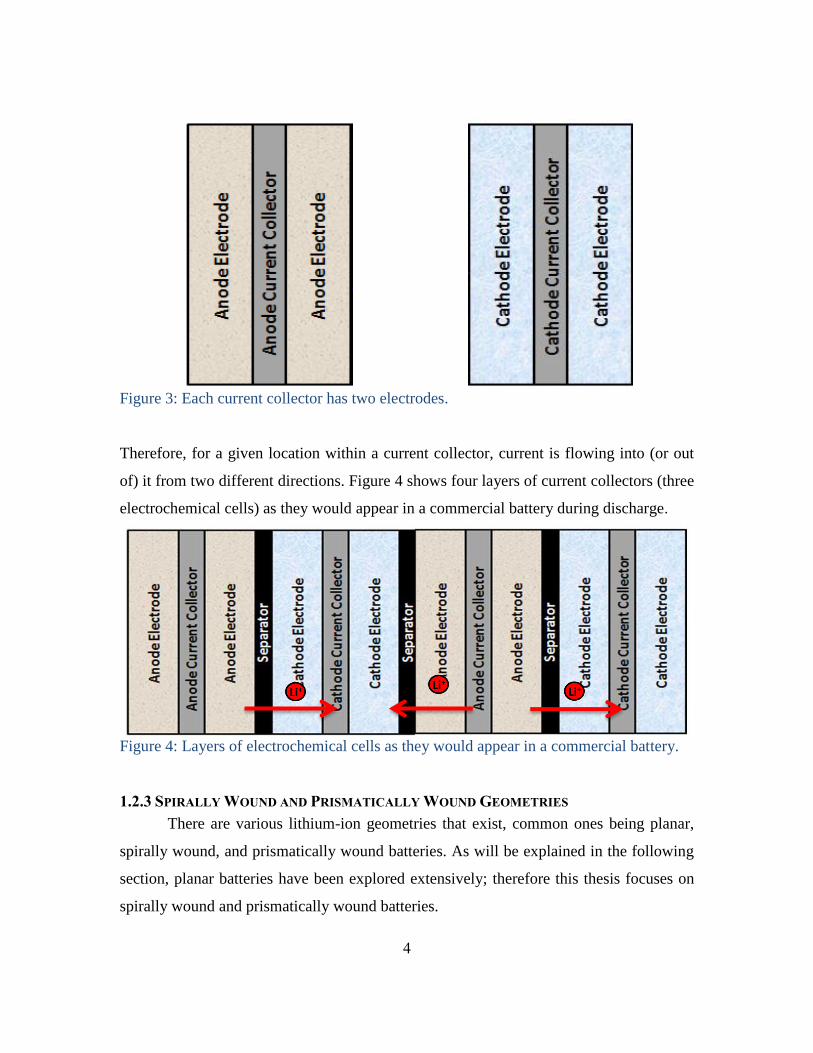
Therefore, for a given location within a current collector, current is flowing into (or out

of) it from two different directions. Figure 4 shows four layers of current collectors (three

electrochemical cells) as they would appear in a commercial battery during discharge.

Figure 4: Layers of electrochemical cells as they would appear in a commercial battery.

1.2.3 SPIRALLY WOUND AND PRISMATICALLY WOUND GEOMETRIES

There are various lithium-ion geometries that exist, common ones being planar,

spirally wound, and prismatically wound batteries. As will be explained in the following

section, planar batteries have been explored extensively; therefore this thesis focuses on

spirally wound and prismatically wound batteries.

5

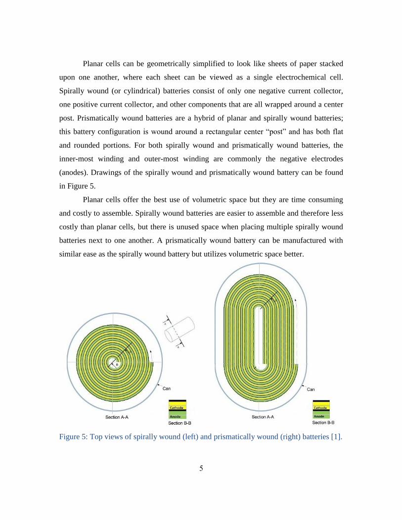
Planar cells can be geometrically simplified to look like sheets of paper stacked

upon one another, where each sheet can be viewed as a single electrochemical cell.

Spirally wound (or cylindrical) batteries consist of only one negative current collector,

one positive current collector, and other components that are all wrapped around a center

post. Prismatically wound batteries are a hybrid of planar and spirally wound batteries;

this battery configuration is wound around a rectangular center “post” and has both flat

and rounded portions. For both spirally wound and prismatically wound batteries, the

inner-most winding and outer-most winding are commonly the negative electrodes

(anodes). Drawings of the spirally wound and prismatically wound battery can be found

in Figure 5.

Planar cells offer the best use of volumetric space but they are time consuming

and costly to assemble. Spirally wound batteries are easier to assemble and therefore less

costly than planar cells, but there is unused space when placing multiple spirally wound

batteries next to one another. A prismatically wound battery can be manufactured with

similar ease as the spirally wound battery but utilizes volumetric space better.

Figure 5: Top views of spirally wound (left) and prismatically wound (right) batteries [1].

6

1.2.4 SPECIFIC MATERIALS

Though other anode materials are being explored currently, graphite (C6) is

commonly used as the negative electrode and is the negative electrode explored in this

thesis. Upon insertion of Li+ into the graphite, the chemical composition is written as

LixC6.

In recent years there have been many breakthroughs on positive electrode

materials. The discovery of layered oxide electrodes by UT’s Dr. John Goodenough

enabled the first widespread use of lithium ion batteries in portable applications

worldwide, with LixCoO2 being the most common electrode material used. Spinel

materials such as LiMn2O4 have been commercialized as well, but recently the olivine

structure has garnered interest. More specifically the olivine structure LiFePO4 (lithium

iron phosphate) has received attention because it is less expensive than most other

electrodes and also allows quicker charging/discharging. It is the positive electrode of a

LiC6/LiPF6/ LiFePO4 cell that is studied in this thesis.

1.3 Prior 3D Modeling of Batteries

Prior work has explored various battery chemistries and geometries and what

current and temperature distributions may look like under different conditions. Early

models focused on only the electrochemical behavior of lithium insertion batteries

utilizing a methodology that was the basis for the electrochemical model used in this

thesis [2][3][4]. Bernardi et al in 1993 modeled the electrochemical reaction of a 2D lead

acid battery isothermally and determined that higher current density will occur at the tabs

of the battery [5].

Soon after, thermal modeling of lithium insertion batteries was conducted by Lee

at al who conducted 3D thermal modeling for large scale electric vehicle batteries, and by

Evans and White who studied 3D heat generation in spirally wound batteries. In both

cases, local variation of heat generation was determined in 3D, but they required pre-

determined inputs for local current density and local potential [6][7]. Verbrugge used a

3D thermal and electrochemical model for a lithium metal vanadium oxide battery that

was accurate under low power conditions. The model was limited because it ignored

7

lithium ion concentration gradients and the current-voltage relationship in the

electrochemical model was treated as being linear [8]. In another study, Baker and

Verbrugge created a perturbation analysis for temperature and current distribution in thin

film batteries but it was only valid for short times [9].

In two studies that utilized finite-element analysis, resistance was specified for

each element in the model and then current distribution and resistive heating were

calculated [10][11]. Bharathan et al treated resistance as constant throughout [10], while

Inui et al allowed resistance to be variable. In Inui’s study of both prismatic and spirally

wound configurations, state of charge and temperature values were derived from

experimental data, and the electrochemical reaction was treated as homogeneous whereas

the thermal model was treated as anisotropic [11].

There is a multitude of electrochemical and thermal models involving the spirally

wound battery configuration. Reimers treated battery impedance as constant in time and

space and solved for current distribution using current collector resistance and

electrochemical cell impedance values; the battery was modeled as if it were unwound

[12]. Harb and LaFollette used porous electrode theory to create a 1D electrochemical

model which was paired with a 2D network of resistors to represent the current

collectors; their study predicted the current distribution within a lead acid battery [13]. In

another study, Harb modeled lithium ion batteries [14], but the methodology in both

studies was different than what is utilized in this thesis. In Harb’s studies, the overall

current or voltage at the tabs was chosen using an educated guess, and the network of

nodes was solved to see if the sum of local current densities (or voltages) equaled the

guessed value; if it was not equal then a new guess was generated [13][14]. In a study by

Heon et al, the effects of current distribution on the temperature field were investigated in

3D, but potential drop across the length of the cell was neglected [15].

Jeon and Baek provided a thermal analysis of cylindrical lithium cobalt oxide and

lithium nickel cobalt manganese batteries during discharge cycles. They used a finite-

element method to determine battery temperatures at various discharge rates but did not

investigate the effects of temperature on local current distribution. Also, the study

8

neglects the existence of tabs [16]. Zhang explored the local thermal properties of a

lithium manganese spinel cylindrical battery during discharge cycles and how they relate

to Li+ concentration across the cell. To determine node spacing, a derivation of

Archimedes’ Spiral Equations was utilized. The study did not look into local current

densities or the effect of tab placement or current collector thickness [17].

There are far fewer studies conducted on prismatic wound batteries. Chen et al

explored the potential for thermal runaway due to overcharge in a prismatically wound

lithium cobalt oxide battery, but it was mostly experimental and did not attempt to map

the temperature or current distribution throughout the cell [18]. Cousseau et al had a

similar experimental exploration of the benefits using a prismatic wound “jellyroll”

configuration. Similar to Chen et al, there was little modeling present and no attempt to

determine localized current and temperature values [19].

Several models demonstrated the importance of coupling good electrochemical

model and thermal models to predict battery performance [20][21][22]. Gerver et al

showed that this coupling is useful in understanding battery safety, optimizing cooling

design and optimization of tab placement and current collector thickness for a prismatic

lithium iron phosphate battery. It explored high power, large scale batteries that can be

utilized in portable applications such as in a hybrid vehicle. As in this thesis, Gerver

utilized a 2D network of resistors paired with a non-linear 1D electrochemical model that

simulated the transient response of a single cell prismatic configuration during charge and

discharge [22]. Gerver’s approach to planar lithium ion batteries is the foundation for the

treatment this thesis takes towards two other battery configurations of the same

chemistry.

This thesis has a 2D network of resistors to model heat generation and current

flow through the current collectors and a 1D non-linear model that represents the

electrochemical reaction occurring in two different configurations of lithium iron

phosphate battery – spirally wound and prismatically wound. The purpose is to show how

temperature and current distribution affect one another in various thermal environments,

tab locations, current collector thicknesses, and C-rates for use in optimizing this

9

particular battery chemistry for use in large scale portable applications such as in an

electric vehicle.

10

CHAPTER 2: MATHEMATICAL MODEL OF WOUND BATTERY

CONFIGURATIONS

2.1 Modeling the Battery as a 3D Network of Resistors:

When operating a battery, only the total current or total voltage across the

terminals is known. Consequently, current density and voltage values for each cell and

for any specific location within that cell are unknown. Locations in which current density

or potential differences are larger in magnitude than the rest of the cell can potentially fail

sooner than the rest of the cell, thereby damaging the entire cell. When trying to optimize

a battery’s performance and durability, it is ideal to have uniform current density and

voltage across each cell; as such, it is necessary to develop a model to determine the local

values. Then one is able to alter properties during cell design to obtain optimal results.

If one wanted to model each location within an electrochemical cell in three

dimensions and then solve for the system of locations, it would be prohibitively time- and

computer- intensive. Instead, by modeling each current collector as a two-dimensional

network of foils connected by resistors, coupled with one dimensional electrochemical

model, the local current and voltage values can be determined accurately and in a

reasonable amount of time. The following treatment follows directly from the work of

Rachel Gerver’s master’s thesis, which developed this solution technique for a planar cell

arrangement. The interested reader should visit her thesis for the full description; Section

2.11 provides an overview of the development to provide context for the current work.

It should be noted that many of the methods used in the following sections are

based on the work Gerver et al implemented for planar lithium iron phosphate batteries,

which in turn is based on the work developed by Doyle, Fuller, and Newman. Both

sources serve as the basis for which the following wound battery models were developed

in the Sections 2.11, 2.2, 2.2.1, 2.2.2, 2.3, 2.3.1, 2.3.2, 2.3.3, 2.3.4, and all three

Appendices.

2.1.1 CURRENT COLLECTOR AND ELECTROCHEMICAL REACTION RESISTORS

Depending on desired model accuracy, the user determines the number of nodes

in two directions, x and y, within each current collector. The current collector is then

11

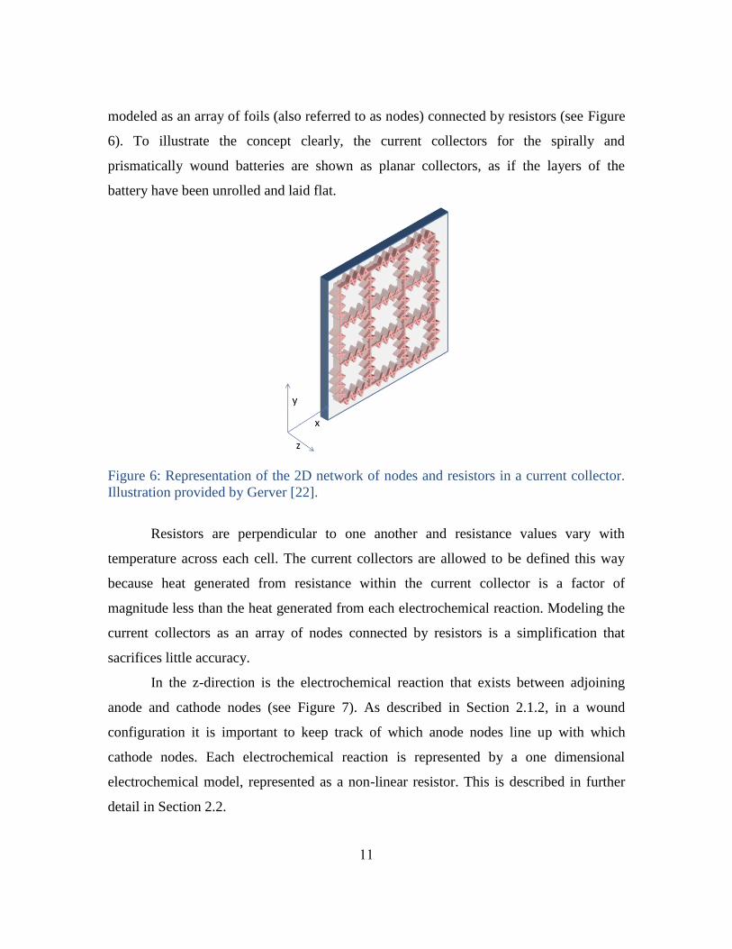
modeled as an array of foils (also referred to as nodes) connected by resistors (see Figure

6). To illustrate the concept clearly, the current collectors for the spirally and

prismatically wound batteries are shown as planar collectors, as if the layers of the

battery have been unrolled and laid flat.

Figure 6: Representation of the 2D network of nodes and resistors in a current collector.

Illustration provided by Gerver [22].

Resistors are perpendicular to one another and resistance values vary with

temperature across each cell. The current collectors are allowed to be defined this way

because heat generated from resistance within the current collector is a factor of

magnitude less than the heat generated from each electrochemical reaction. Modeling the

current collectors as an array of nodes connected by resistors is a simplification that

sacrifices little accuracy.

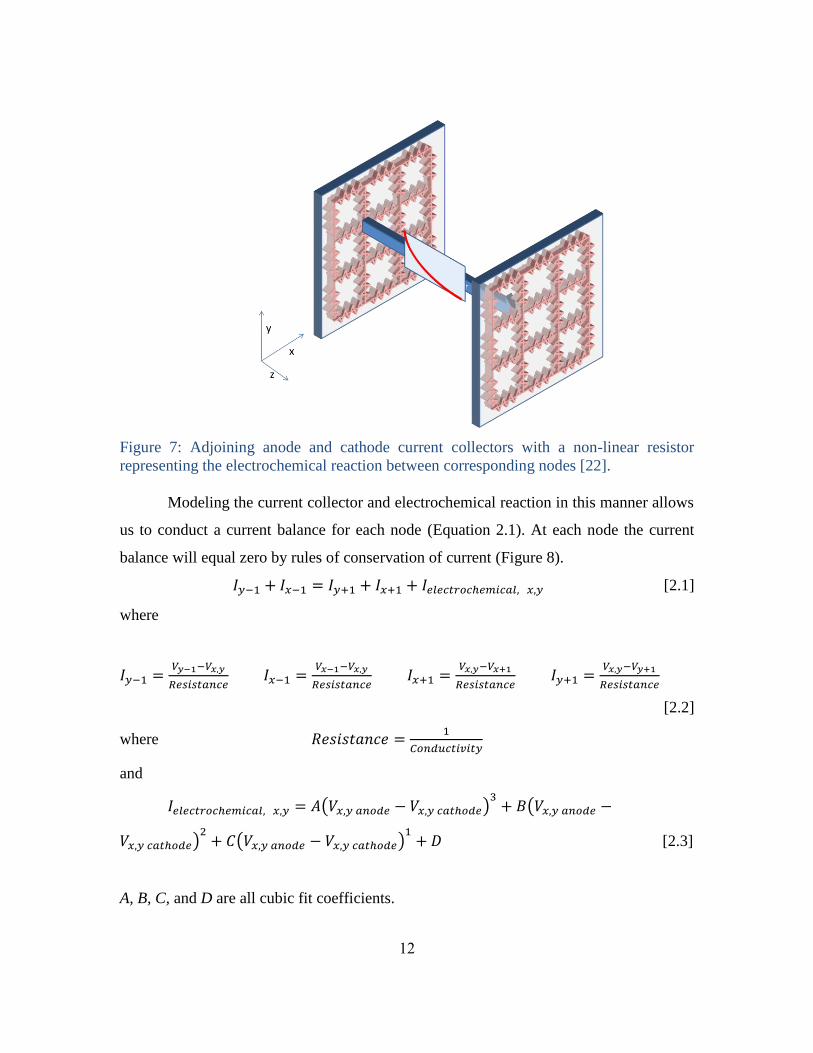
In the z-direction is the electrochemical reaction that exists between adjoining

anode and cathode nodes (see Figure 7). As described in Section 2.1.2, in a wound

configuration it is important to keep track of which anode nodes line up with which

cathode nodes. Each electrochemical reaction is represented by a one dimensional

electrochemical model, represented as a non-linear resistor. This is described in further

detail in Section 2.2.

12

Figure 7: Adjoining anode and cathode current collectors with a non-linear resistor

representing the electrochemical reaction between corresponding nodes [22].

Modeling the current collector and electrochemical reaction in this manner allows

us to conduct a current balance for each node (Equation 2.1). At each node the current

balance will equal zero by rules of conservation of current (Figure 8).

[2.1]

where

[2.2]

where

and

( ) (

) ( )

[2.3]

A, B, C, and D are all cubic fit coefficients.

13

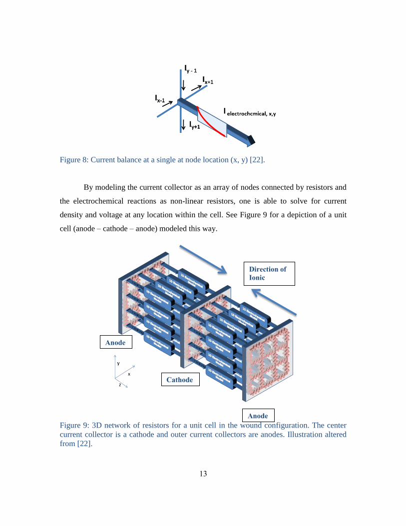
Figure 8: Current balance at a single at node location (x, y) [22].

By modeling the current collector as an array of nodes connected by resistors and

the electrochemical reactions as non-linear resistors, one is able to solve for current

density and voltage at any location within the cell. See Figure 9 for a depiction of a unit

cell (anode – cathode – anode) modeled this way.

Figure 9: 3D network of resistors for a unit cell in the wound configuration. The center

current collector is a cathode and outer current collectors are anodes. Illustration altered

from [22].

Anode

Anode

Cathode

Direction of

Ionic

Current

14

Cathode nodes

2.1.2 ALIGNMENT OF NODES IN WOUND CONFIGURATIONS

Thus far, each of the previous four figures displayed a simplified view of the 3D

network of resistors; this is how they would appear in a planar cell. In a battery that is

wound, there is a slight difference in alignment of nodes due to the curvature and winding

of the components.

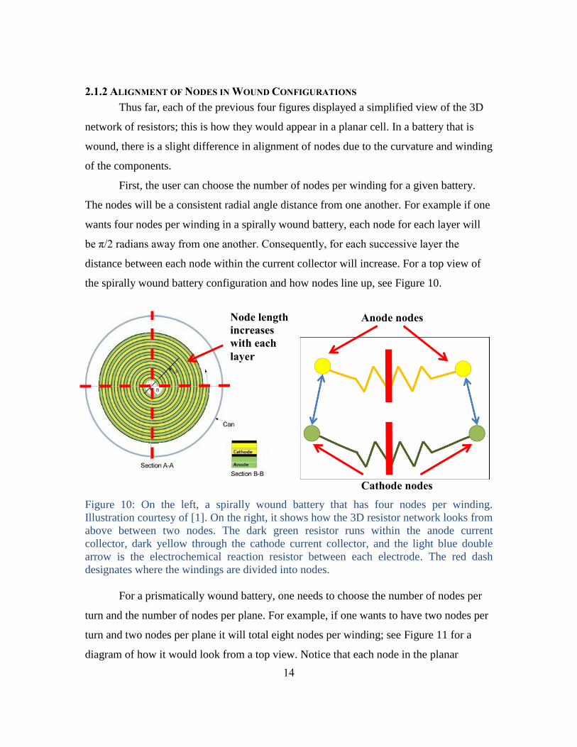
First, the user can choose the number of nodes per winding for a given battery.

The nodes will be a consistent radial angle distance from one another. For example if one

wants four nodes per winding in a spirally wound battery, each node for each layer will

be π/2 radians away from one another. Consequently, for each successive layer the

distance between each node within the current collector will increase. For a top view of

the spirally wound battery configuration and how nodes line up, see Figure 10.

Figure 10: On the left, a spirally wound battery that has four nodes per winding.

Illustration courtesy of [1]. On the right, it shows how the 3D resistor network looks from

above between two nodes. The dark green resistor runs within the anode current

collector, dark yellow through the cathode current collector, and the light blue double

arrow is the electrochemical reaction resistor between each electrode. The red dash

designates where the windings are divided into nodes.

For a prismatically wound battery, one needs to choose the number of nodes per

turn and the number of nodes per plane. For example, if one wants to have two nodes per

turn and two nodes per plane it will total eight nodes per winding; see Figure 11 for a

diagram of how it would look from a top view. Notice that each node in the planar

Node length

increases

with each

layer

Anode nodes

15

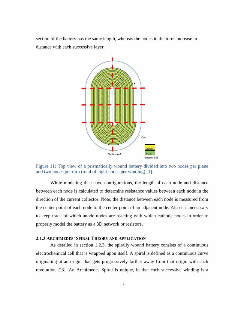
section of the battery has the same length, whereas the nodes in the turns increase in

distance with each successive layer.

Figure 11: Top view of a prismatically wound battery divided into two nodes per plane

and two nodes per turn (total of eight nodes per winding) [1].

While modeling these two configurations, the length of each node and distance

between each node is calculated to determine resistance values between each node in the

direction of the current collector. Note, the distance between each node is measured from

the center point of each node to the center point of an adjacent node. Also it is necessary

to keep track of which anode nodes are reacting with which cathode nodes in order to

properly model the battery as a 3D network or resistors.

2.1.3 ARCHIMEDES’ SPIRAL THEORY AND APPLICATION

As detailed in section 1.2.3, the spirally wound battery consists of a continuous

electrochemical cell that is wrapped upon itself. A spiral is defined as a continuous curve

originating at an origin that gets progressively farther away from that origin with each

revolution [23]. An Archimedes Spiral is unique, in that each successive winding is a

16

constant distance δ from the previous winding. The spiral is named after the Greek

mathematician, Archimedes, who discussed this type of spiral in his 225BC publication

titled On Spirals [25].

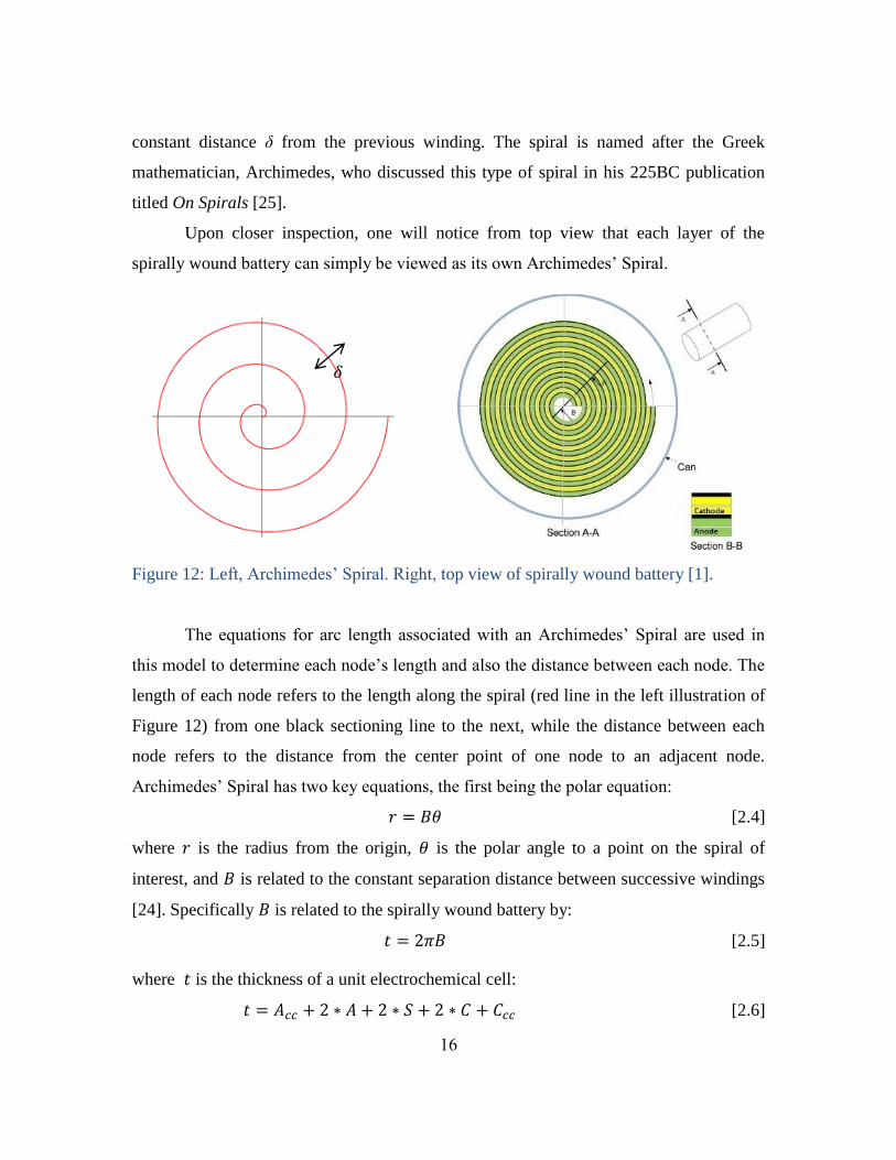
Upon closer inspection, one will notice from top view that each layer of the

spirally wound battery can simply be viewed as its own Archimedes’ Spiral.

Figure 12: Left, Archimedes’ Spiral. Right, top view of spirally wound battery [1].

The equations for arc length associated with an Archimedes’ Spiral are used in

this model to determine each node’s length and also the distance between each node. The

length of each node refers to the length along the spiral (red line in the left illustration of

Figure 12) from one black sectioning line to the next, while the distance between each

node refers to the distance from the center point of one node to an adjacent node.

Archimedes’ Spiral has two key equations, the first being the polar equation:

[2.4]

where is the radius from the origin, is the polar angle to a point on the spiral of

interest, and is related to the constant separation distance between successive windings

[24]. Specifically is related to the spirally wound battery by:

[2.5]

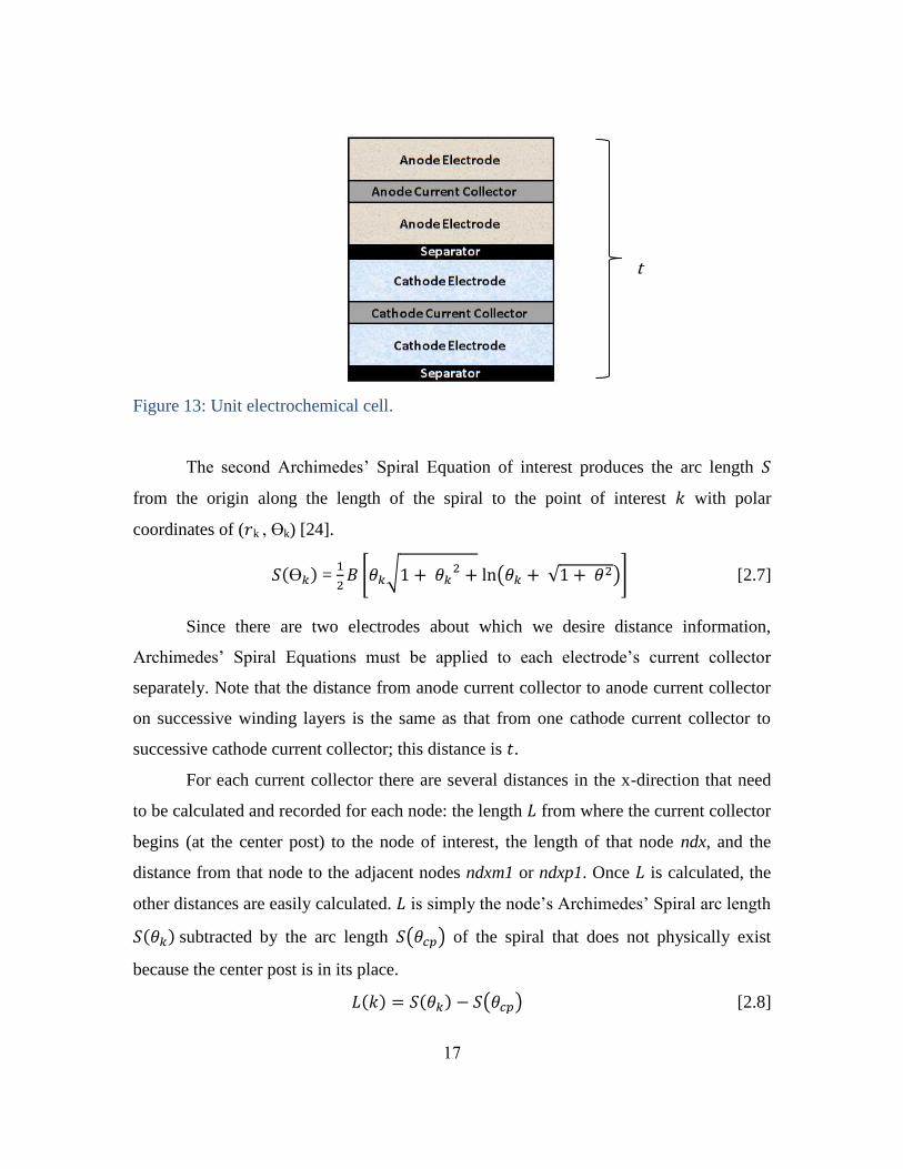
where is the thickness of a unit electrochemical cell:

[2.6]

𝛿

17

Figure 13: Unit electrochemical cell.

The second Archimedes’ Spiral Equation of interest produces the arc length

from the origin along the length of the spiral to the point of interest with polar

coordinates of ( k , ϴk) [24].

(ϴ ) =

[ √

( √ )] [2.7]

Since there are two electrodes about which we desire distance information,

Archimedes’ Spiral Equations must be applied to each electrode’s current collector

separately. Note that the distance from anode current collector to anode current collector

on successive winding layers is the same as that from one cathode current collector to

successive cathode current collector; this distance is .

For each current collector there are several distances in the x-direction that need

to be calculated and recorded for each node: the length from where the current collector

begins (at the center post) to the node of interest, the length of that node ndx, and the

distance from that node to the adjacent nodes ndxm1 or ndxp1. Once is calculated, the

other distances are easily calculated. is simply the node’s Archimedes’ Spiral arc length

( ) subtracted by the arc length ( ) of the spiral that does not physically exist

because the center post is in its place.

( ) ( ) ( ) [2.8]

t

18

where

Anode:

Cathode:

Since we want to find the Archimedes’ Spiral arc length to the center of a particular

node, we must subtract ½ of a nodal rotation to determine .

Anode: ( ) [ ( ) ]

Cathode: ( ) [ ( ) ] [2.9]

Once ( ) is obtained, each node’s length and distance between adjacent nodes is

calculated:

( ) ( )

( ) ( )

( ) [2.10]

With these distances, one can easily calculate the area per node and volume per node. All

values are useful in calculating conductivity, current density, and heat generation.

List of Symbols

Acc Anode current collector thickness

Ccc Cathode current collector thickness

A Anode electrode thickness

C Cathode electrode thickness

S Separator thickness

t Unit electrochemical cell thickness

k Cell node

npw Nodes per winding

ny Position in the y direction

nxanode Position in the x direction on the anode

nxcathode Position in the x direction on the cathode

19

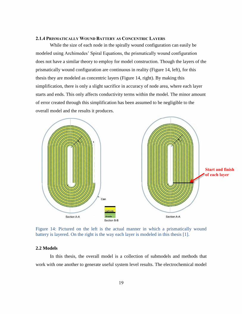
2.1.4 PRISMATICALLY WOUND BATTERY AS CONCENTRIC LAYERS

While the size of each node in the spirally wound configuration can easily be

modeled using Archimedes’ Spiral Equations, the prismatically wound configuration

does not have a similar theory to employ for model construction. Though the layers of the

prismatically wound configuration are continuous in reality (Figure 14, left), for this

thesis they are modeled as concentric layers (Figure 14, right). By making this

simplification, there is only a slight sacrifice in accuracy of node area, where each layer

starts and ends. This only affects conductivity terms within the model. The minor amount

of error created through this simplification has been assumed to be negligible to the

overall model and the results it produces.

Figure 14: Pictured on the left is the actual manner in which a prismatically wound

battery is layered. On the right is the way each layer is modeled in this thesis [1].

2.2 Models

In this thesis, the overall model is a collection of submodels and methods that

work with one another to generate useful system level results. The electrochemical model

Start and finish

of each layer

20

is coupled with a thermal model and solved using numerical methods. Sections 2.2.1 and

2.2.2 detail each model and their coupling in greater detail.

2.2.1 ELECTROCHEMICAL MODEL

For each anode-cathode node pairing within a cell, the current-voltage profile is

needed in order to have a functional model. Rather than sweeping through a range of

voltages and currents for each node at every time step (which is both time consuming and

computationally intensive), the goal is to create polynomial fit (cubic) current-voltage

curves for each node that can be assumed for subsequent time steps. This is done by

running each node at several different current densities over the same time step using

initial conditions dictated by the user. This will provide the voltage across the cell

(between anode and cathode) at each current density. Then, a cubic fit curve is applied to

the results to obtain an equation that represents each node’s electrochemical reaction. The

equation, first mentioned in section 2.1.1, generates electrochemical current as a function

of voltage (equation [2.3]).

When operating a battery, the current-voltage cubic curve will shift based upon

the state of charge. With each successive time step, the curve will shift downward or

upward by ΔI depending on if the battery is charging or discharging. The value for ΔI is

approximated from user inputs and is constant throughout the simulation. For a given

time step, the equation to generate Ielectrochemical at each node comes from the previous time

step, with the only difference between time steps being that it has been shifted by ΔI.

Next, these Ielectrochemical values are compared to a select few Ielectrochemical values that have

been generated directly from the electrochemical model. If the comparison is within a

preset tolerance, then the shift is accepted and that cubic curve is used. If not, then the

sweeping process using the full electrochemical model (running each node at several

current densities) is performed again for that time step.

The electrochemical model is based on porous electrode theory for lithium ion

batteries developed by Doyle, Fuller and Newman. It is described in further detail in

Appendix B. Simply stated, it makes use of six electrochemical theory equations to solve

for six unknown variables. The unknown variables needed to generate the current-voltage

21

curve are potential in the solid (φ1), potential in the solution (φ2), current in the solid (i2),

rate of reaction (in), concentration of Li+ in solution (c), and concentration of Li

+ at the

electrode surface (cs). The six equations, derived and proven in electrochemical theory,

are the Butler-Volmer equation, from concentrated solution theory, from porous electrode

theory, a solid potential equation, a solution potential equation, and a solution current

equation. The six unknowns in the six equations are solved numerically by the Newton

Raphson method (described in Section 2.3.4). For each time step the thermal model is

coupled with the electrochemical model to determine the impact of temperature on

electrochemical performance and vice versa.

2.2.2 THERMAL MODEL AND COUPLING WITH ELECTROCHEMICAL MODEL

Under both charge and discharge, a battery will generate heat in two ways. One,

there is irreversible heat generation due to cell resistance, both across the electrochemical

cell and within the current collectors; it is associated with heat capacity, heat transfer and

heat generation all in relation to the structure of the battery and the materials used. Two,

there is reversible heat generation due to entropy of the electrochemical reaction itself,

which can be exothermic or endothermic depending on whether the battery is charging or

discharging; this is associated with ionization on one electrode, transfer of ions across the

cell, and joining of ions with electrons at the opposite electrode. This thermal model

accounts for both of these sources of heat.

This is described in further detail in Appendix B, but simply put heat generation

due to cell resistance is calculated at each node and heat generation by the

electrochemical reaction is calculated for each anode-cathode node pairing. Using these

two heat generation values, temperature is then calculated for each node pairing. These

temperature values for each node pairing are then used as inputs to the electrochemical

model on the following time step.

This model assumes a quasi-steady state temperature for each time step. The

model user decides the length of each time step, but the time steps selected to generate

results for this thesis are one second long. This means that the temperature is considered

constant, but it acknowledges that the electrochemical response is on a different time

22

scale than the thermal response. Also it is assumed in the electrochemical model that the

input temperature is constant across the five layers of the cell (anode current collector,

anode electrode, separator, cathode electrode, and cathode current collector).

2.3 Numerical Methods

As mentioned in 2.2.1, the six unknown electrochemical variables are solved for

using six electrochemical reaction equations and the Newton-Raphson method. For this

thesis, the Newton-Raphson method is also used in the thermal model and in the three

dimensional current balance analysis, and the method is described in full detail in

Electrochemical Systems [26].

Specifically, four of the electrochemical reaction equations are converted from

partial differential equations to finite difference approximations (described in Section

2.3.1) before being solved using the Newton-Raphson method. The other two equations,

which have to do with concentration of lithium in solution and solid, are handled in a

different manner as detailed in Sections 2.3.2 and 2.3.3.

2.3.1 FINITE DIFFERENCE METHOD

The four partial differential equations are converted using the finite difference

method. Examples are as follows:

dc

dx| -

( ) ( )

( ) [2.11]

|

( ) ( ) ( )

( ) [2.12]

Here c is the variable being solved, j is the mesh point, and h is the mesh spacing [22].

The Crank-Nicolson method is used for differential equations that are time

dependent. This method is implicit and unconditionally stable with respect to time. An

example is as follows:

[2.13]

23

(

)

[2.14]

Here, n is the time step number, Δt is the time step size, D is a coefficient that can vary

with time, and the other variables are as described for equations 2.11 and 2.12 [22].

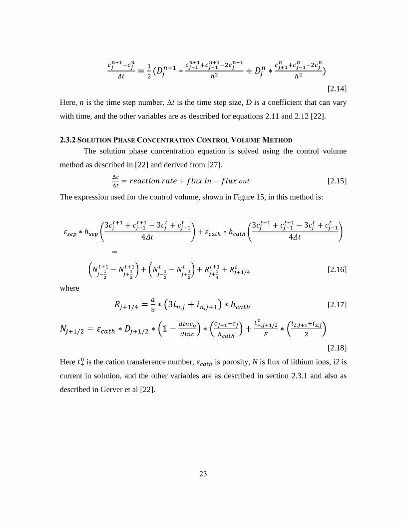
2.3.2 SOLUTION PHASE CONCENTRATION CONTROL VOLUME METHOD

The solution phase concentration equation is solved using the control volume

method as described in [22] and derived from [27].

[2.15]

The expression used for the control volume, shown in Figure 15, in this method is:

(

) (

)

(

) (

)

[2.16]

where

( ) [2.17]

(

) (

)

(

)

[2.18]

Here

is the cation transference number, is porosity, N is flux of lithium ions, i2 is

current in solution, and the other variables are as described in section 2.3.1 and also as

described in Gerver et al [22].

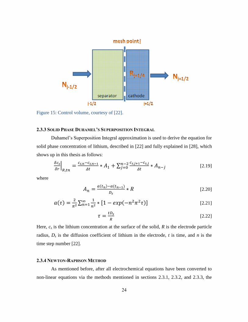
24

Figure 15: Control volume, courtesy of [22].

2.3.3 SOLID PHASE DUHAMEL’S SUPERPOSITION INTEGRAL

Duhamel’s Superposition Integral approximation is used to derive the equation for

solid phase concentration of lithium, described in [22] and fully explained in [28], which

shows up in this thesis as follows:

|

∑

[2.19]

where

( ) ( )

[2.20]

( )

∑

[ ( )]

[2.21]

[2.22]

Here, cs is the lithium concentration at the surface of the solid, R is the electrode particle

radius, Ds is the diffusion coefficient of lithium in the electrode, t is time, and n is the

time step number [22].

2.3.4 NEWTON-RAPHSON METHOD

As mentioned before, after all electrochemical equations have been converted to

non-linear equations via the methods mentioned in sections 2.3.1, 2.3.2, and 2.3.3, the

25

Newton-Raphson method is applied. It is also applied to the thermal model and the three

dimensional current balance conducted at each node.

In this paragraph, a single unknown and single equation is explained to show the

Newton-Raphson method at its simplest state. In this method, the term g(c) is created to

solve for c; c will be an accurate solution when g(c) = 0. First, g(c) is expanded as a

Taylor series:

( ) ( )

| ( ) [2.23]

For this method to converge and produce desired results, a good initial guess for c0 is

necessary. Neglecting higher order terms and setting g(c) = 0, equation 2.23 becomes:

( )

⁄ |

[2.24]

The new term, c, provides a more accurate approximation for the solution, and as one

repeats this exercise it will converge to an accurate solution [26].

With several unknowns, a multidimensional Taylor series is used. The function of

which we are seeking a solution will have more than one variable:

( )

where n is the number of unknown variables, j is the number of mesh points, and k is the

designation for a particular unknown variable. Expanded into a Taylor series and the non-

linear terms neglected:

∑

| ∑

| ∑

| [2.25]

Equation 15 can be written:

∑ (

) [2.26]

Equation 16 can then be written as a tridiagonal matrix (with respect to j):

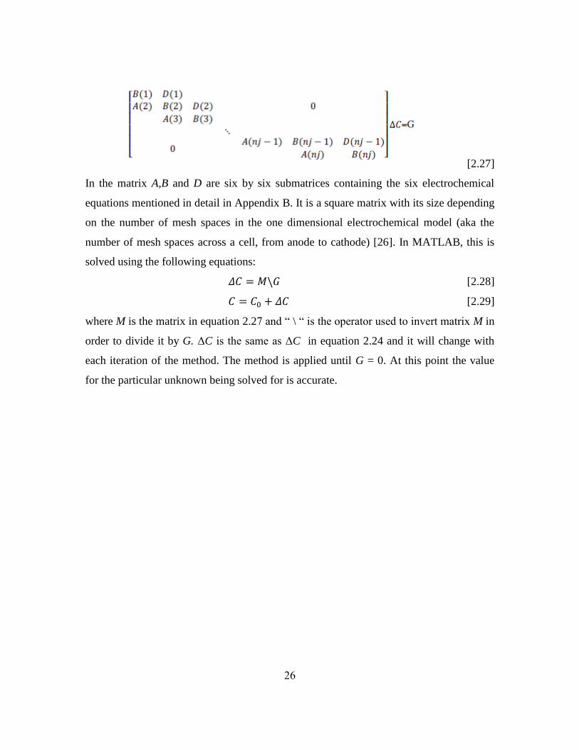
26

[2.27]

In the matrix A,B and D are six by six submatrices containing the six electrochemical

equations mentioned in detail in Appendix B. It is a square matrix with its size depending

on the number of mesh spaces in the one dimensional electrochemical model (aka the

number of mesh spaces across a cell, from anode to cathode) [26]. In MATLAB, this is

solved using the following equations:

[2.28]

[2.29]

where M is the matrix in equation 2.27 and “ \ “ is the operator used to invert matrix M in

order to divide it by G. ΔC is the same as ΔC in equation 2.24 and it will change with

each iteration of the method. The method is applied until G = 0. At this point the value

for the particular unknown being solved for is accurate.

27

CHAPTER 3: NUMERICAL RESULTS

3.1 Design Optimization

For each configuration, there are various design considerations that will affect battery

performance, durability, and safety. In this thesis tab location, cooling environment, current

collector thickness, and risk of lithium plating are all explored in depth using the models

described in Chapter 2.

In all of Chapter 3, a “base case” configuration is referred to multiple times. This refers to

the specifications detailed in Appendix A for both the spirally wound and prismatically wound

configurations. Unless otherwise noted, these specifications are used for the study.

Also it should be noted that many results are represented visually using color mapping. In

all of the figures that display results, the minima and maxima used for the scale are the same for

all cases that have been explored. This is done to make it easy for the reader to compare each

different case (i.e. the temperature scale used for adiabatic, isothermal, air cooled and liquid

cooled is that of the adiabatic case since it has the largest temperature range. All other cases use

the same range so one can see how much better liquid cools down the battery versus adiabatic).

Lastly, the design considerations explored in this thesis are the same as those explored in

Gerver et al. This was down so as to compare all three configurations (and how the design

considerations affect each) easily.

3.1.1: SINGLE TAB VERSUS MULTIPLE TAB COMPARISON

Within a battery, all current that is generated flows to the aptly named current collectors.

To extract the current from the battery, current collector tabs are utilized to connect the current

collectors to the external circuit. As will be seen in this section, tab location(s) affects the current

density and temperature distribution throughout the cell, which in turn affects the overall

performance and durability of the battery.

It is desirable to have as close to uniform current density and temperature as possible

(achieved by tabs spanning the entire length of each current collector), but it is also desirable to

limit the amount of non-active material in portable batteries (achieved by as little tab material as

possible). Therefore there is an opportunity for optimization by seeking to have uniform current

density and temperature while limiting amount of tab material. Tab placement and number of tabs

is an important design parameter for every battery and will be explored in this section.

28

3.1.1.1 Spiral Configuration – Tabs

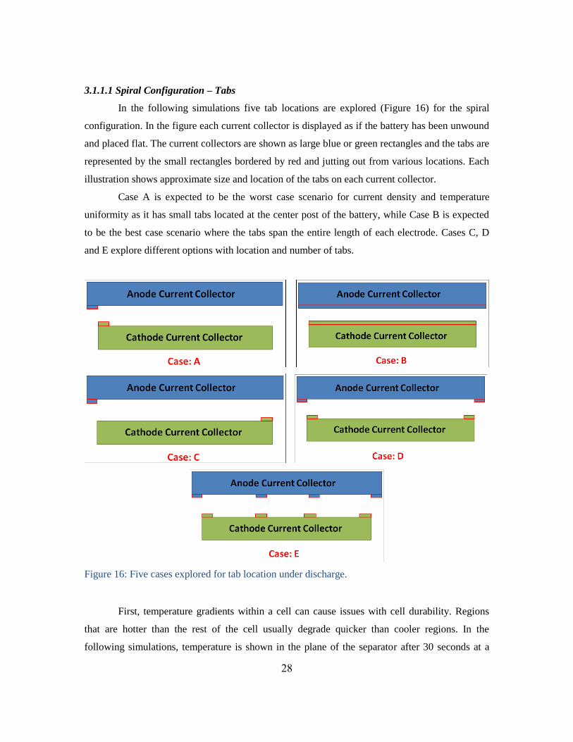
In the following simulations five tab locations are explored (Figure 16) for the spiral

configuration. In the figure each current collector is displayed as if the battery has been unwound

and placed flat. The current collectors are shown as large blue or green rectangles and the tabs are

represented by the small rectangles bordered by red and jutting out from various locations. Each

illustration shows approximate size and location of the tabs on each current collector.

Case A is expected to be the worst case scenario for current density and temperature

uniformity as it has small tabs located at the center post of the battery, while Case B is expected

to be the best case scenario where the tabs span the entire length of each electrode. Cases C, D

and E explore different options with location and number of tabs.

Figure 16: Five cases explored for tab location under discharge.

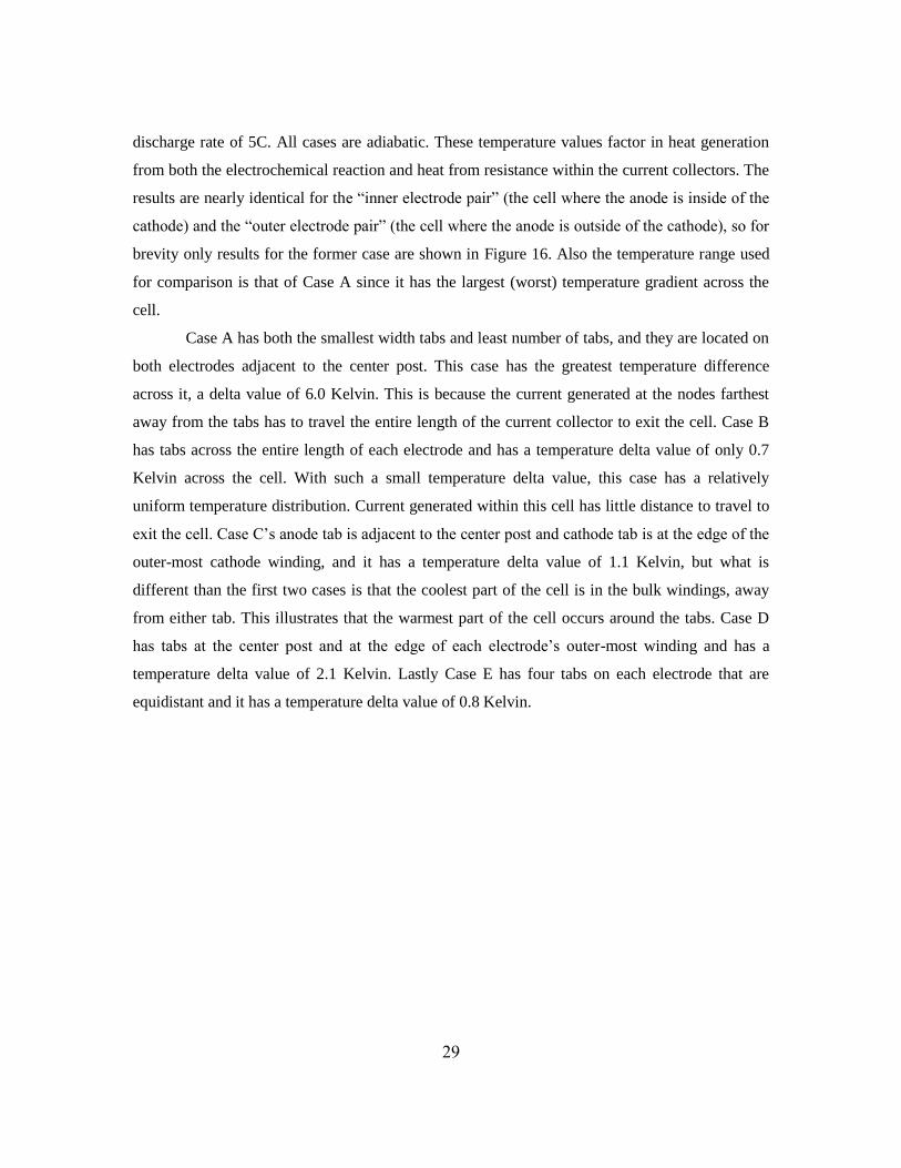
First, temperature gradients within a cell can cause issues with cell durability. Regions

that are hotter than the rest of the cell usually degrade quicker than cooler regions. In the

following simulations, temperature is shown in the plane of the separator after 30 seconds at a

29

discharge rate of 5C. All cases are adiabatic. These temperature values factor in heat generation

from both the electrochemical reaction and heat from resistance within the current collectors. The

results are nearly identical for the “inner electrode pair” (the cell where the anode is inside of the

cathode) and the “outer electrode pair” (the cell where the anode is outside of the cathode), so for

brevity only results for the former case are shown in Figure 16. Also the temperature range used

for comparison is that of Case A since it has the largest (worst) temperature gradient across the

cell.

Case A has both the smallest width tabs and least number of tabs, and they are located on

both electrodes adjacent to the center post. This case has the greatest temperature difference

across it, a delta value of 6.0 Kelvin. This is because the current generated at the nodes farthest

away from the tabs has to travel the entire length of the current collector to exit the cell. Case B

has tabs across the entire length of each electrode and has a temperature delta value of only 0.7

Kelvin across the cell. With such a small temperature delta value, this case has a relatively

uniform temperature distribution. Current generated within this cell has little distance to travel to

exit the cell. Case C’s anode tab is adjacent to the center post and cathode tab is at the edge of the

outer-most cathode winding, and it has a temperature delta value of 1.1 Kelvin, but what is

different than the first two cases is that the coolest part of the cell is in the bulk windings, away

from either tab. This illustrates that the warmest part of the cell occurs around the tabs. Case D

has tabs at the center post and at the edge of each electrode’s outer-most winding and has a

temperature delta value of 2.1 Kelvin. Lastly Case E has four tabs on each electrode that are

equidistant and it has a temperature delta value of 0.8 Kelvin.

30

Figure 17: Temperature versus position for 5 different tab locations at a discharge rate of 5C.

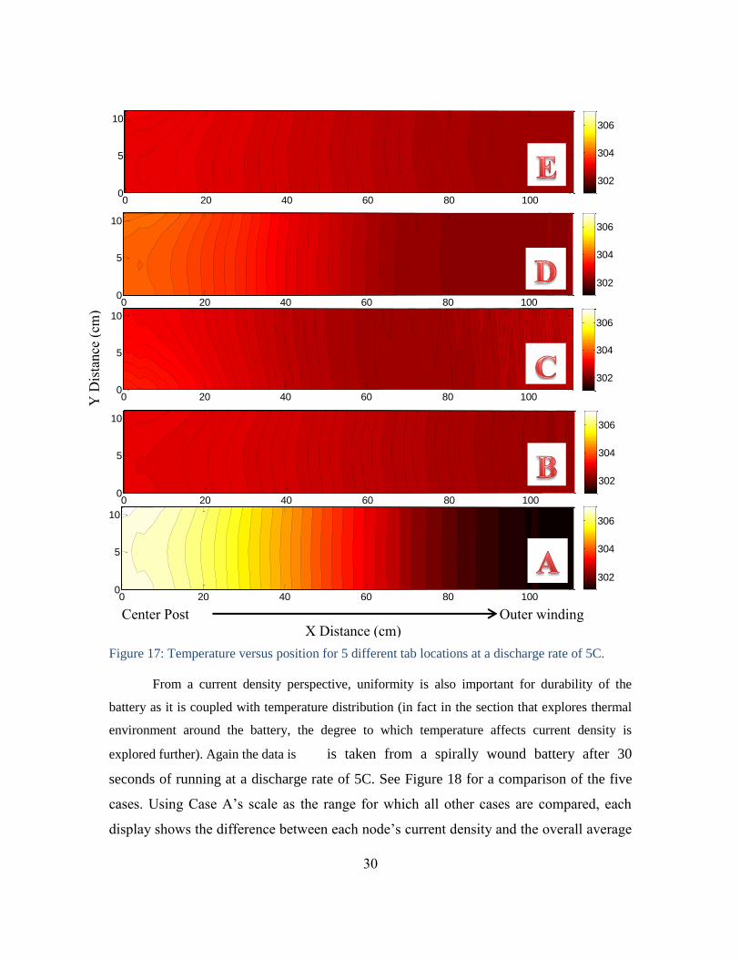
From a current density perspective, uniformity is also important for durability of the

battery as it is coupled with temperature distribution (in fact in the section that explores thermal

environment around the battery, the degree to which temperature affects current density is

explored further). Again the data is is taken from a spirally wound battery after 30

seconds of running at a discharge rate of 5C. See Figure 18 for a comparison of the five

cases. Using Case A’s scale as the range for which all other cases are compared, each

display shows the difference between each node’s current density and the overall average

0 20 40 60 80 1000

5

10

302

304

306

0 20 40 60 80 1000

5

10

302

304

306

0 20 40 60 80 1000

5

10

302

304

306

0 20 40 60 80 1000

5

10

302

304

306

0 20 40 60 80 1000

5

10

302

304

306

Center Post Outer winding

X Distance (cm)

Y D

ista

nce

(cm

)

31

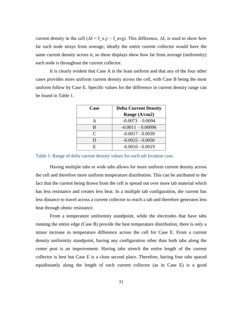
current density in the cell (ΔI I_x,y – I_avg). This difference, ΔI, is used to show how

far each node strays from average; ideally the entire current collector would have the

same current density across it, so these displays show how far from average (uniformity)

each node is throughout the current collector.

It is clearly evident that Case A is the least uniform and that any of the four other

cases provides more uniform current density across the cell, with Case B being the most

uniform follow by Case E. Specific values for the difference in current density range can

be found in Table 1.

Case Delta Current Density

Range (A/cm2)

A -0.0073 – 0.0094

B -0.0011 – 0.00096

C -0.0017 - 0.0039

D -0.0025 - 0.0050

E -0.0010 - 0.0019

Table 1: Range of delta current density values for each tab location case.

Having multiple tabs or wide tabs allows for more uniform current density across

the cell and therefore more uniform temperature distribution. This can be attributed to the

fact that the current being drawn from the cell is spread out over more tab material which

has less resistance and creates less heat. In a multiple tab configuration, the current has

less distance to travel across a current collector to reach a tab and therefore generates less

heat through ohmic resistance.

From a temperature uniformity standpoint, while the electrodes that have tabs

running the entire edge (Case B) provide the best temperature distribution, there is only a

minor increase in temperature difference across the cell for Case E. From a current

density uniformity standpoint, having any configuration other than both tabs along the

center post is an improvement. Having tabs stretch the entire length of the current

collector is best but Case E is a close second place. Therefore, having four tabs spaced

equidistantly along the length of each current collector (as in Case E) is a good

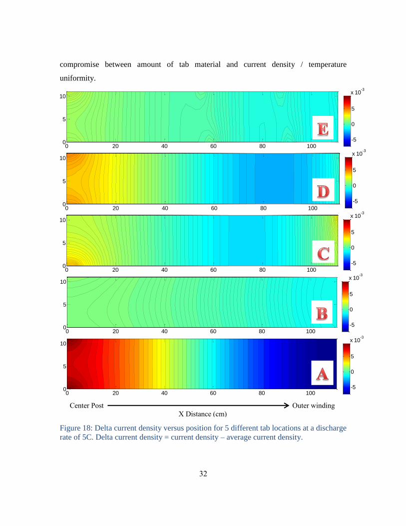
32

compromise between amount of tab material and current density / temperature

uniformity.

Figure 18: Delta current density versus position for 5 different tab locations at a discharge

rate of 5C. Delta current density = current density – average current density.

0 20 40 60 80 1000

5

10

-5

0

5

x 10-3

0 20 40 60 80 1000

5

10

-5

0

5

x 10-3

0 20 40 60 80 1000

5

10

-5

0

5

x 10-3

0 20 40 60 80 1000

5

10

-5

0

5

x 10-3

0 20 40 60 80 1000

5

10

-5

0

5

x 10-3

Center Post Outer winding

X Distance (cm)

33

One last point is that this tab location exploration drives where the current will

exit/enter the cell. By comparing the results in Figure 18 to Figure 17, it is evident that

regions in which there is higher current density will in fact have an increased local

temperature and vice versa. This makes sense since the electrochemical and thermal

models are coupled, but it is important to determine if one parameter causes the other or

if they are perfectly coupled. Since these simulations control the current density flowing

through the tabs, one is able to conclude that increased current density will lead to

increased temperatures. In a later section that explores the thermal environment around

the battery, the degree to which temperature change affects current density is explored.

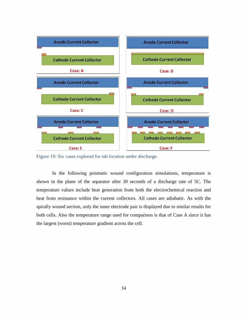
3.1.1.2 Prismatically Wound Configuration – Tabs

In the following simulations six tab locations are explored. See Figure 19 for

illustrations of tab placement, where each current collector is displayed as if the battery

has been unwound and placed flat. The current collectors are shown as large rectangles

and the tabs are represented by the short rectangles bordered by red and jutting out from

various locations. Each illustration shows approximate size and location of the tabs on

each current collector.

Similar to the spirally wound configuration simulations, Case A is expected to be

the worst case scenario as it has small tabs located at the center post of the battery, while

Case B is expected to be the best case scenario where the tabs span the entire length of

each electrode. Cases C, D, E, and F explore different options with location and number

of tabs.

34

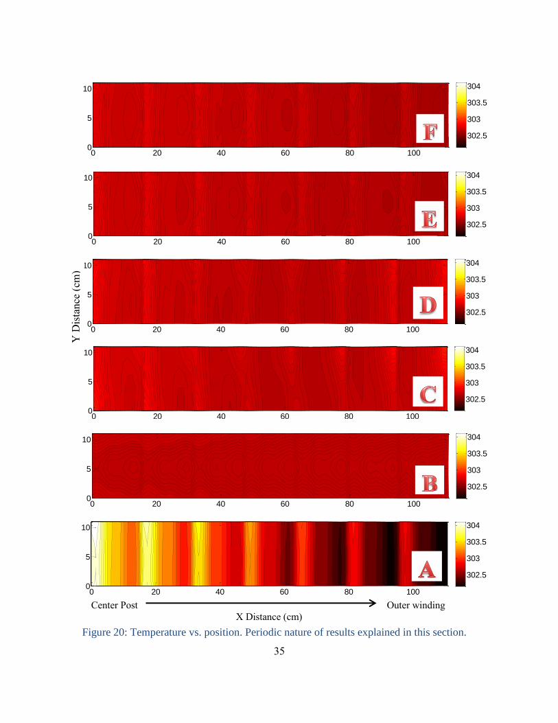
Figure 19: Six cases explored for tab location under discharge.

In the following prismatic wound configuration simulations, temperature is

shown in the plane of the separator after 30 seconds of a discharge rate of 5C. The

temperature values include heat generation from both the electrochemical reaction and

heat from resistance within the current collectors. All cases are adiabatic. As with the

spirally wound section, only the inner electrode pair is displayed due to similar results for

both cells. Also the temperature range used for comparison is that of Case A since it has

the largest (worst) temperature gradient across the cell.

35

Figure 20: Temperature vs. position. Periodic nature of results explained in this section.

0 20 40 60 80 1000

5

10

302.5

303

303.5

304

0 20 40 60 80 1000

5

10

302.5

303

303.5

304

0 20 40 60 80 1000

5

10

302.5

303

303.5

304

0 20 40 60 80 1000

5

10

302.5

303

303.5

304

0 20 40 60 80 1000

5

10

302.5

303

303.5

304

0 20 40 60 80 1000

5

10

302.5

303

303.5

304

Center Post Outer winding

X Distance (cm)

Y D

ista

nce

(cm

)

36

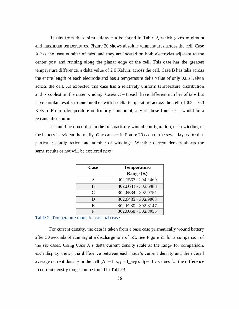
Results from these simulations can be found in Table 2, which gives minimum

and maximum temperatures. Figure 20 shows absolute temperatures across the cell. Case

A has the least number of tabs, and they are located on both electrodes adjacent to the

center post and running along the planar edge of the cell. This case has the greatest

temperature difference, a delta value of 2.0 Kelvin, across the cell. Case B has tabs across

the entire length of each electrode and has a temperature delta value of only 0.03 Kelvin

across the cell. As expected this case has a relatively uniform temperature distribution

and is coolest on the outer winding. Cases C – F each have different number of tabs but

have similar results to one another with a delta temperature across the cell of 0.2 – 0.3

Kelvin. From a temperature uniformity standpoint, any of these four cases would be a

reasonable solution.

It should be noted that in the prismatically wound configuration, each winding of

the battery is evident thermally. One can see in Figure 20 each of the seven layers for that

particular configuration and number of windings. Whether current density shows the

same results or not will be explored next.

Case Temperature

Range (K)

A 302.1567 - 304.2460

B 302.6683 - 302.6988

C 302.6534 - 302.9751

D 302.6435 - 302.9065

E 302.6230 - 302.8147

F 302.6058 - 302.8055

Table 2: Temperature range for each tab case.

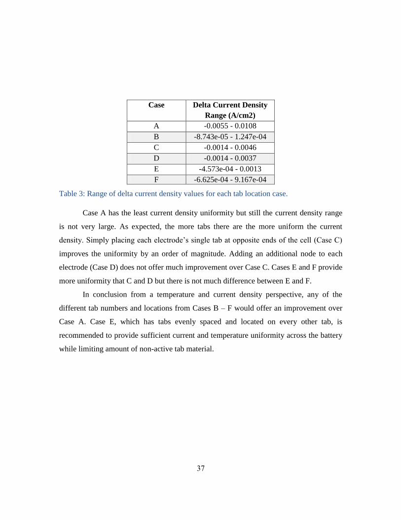
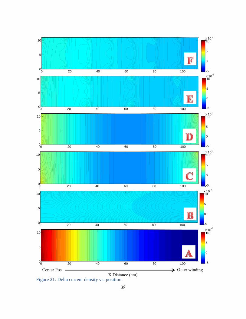
For current density, the data is taken from a base case prismatically wound battery

after 30 seconds of running at a discharge rate of 5C. See Figure 21 for a comparison of

the six cases. Using Case A’s delta current density scale as the range for comparison,

each display shows the difference between each node’s current density and the overall

average current density in the cell (ΔI I_x,y – I_avg). Specific values for the difference

in current density range can be found in Table 3.

37

Case Delta Current Density

Range (A/cm2)

A -0.0055 - 0.0108

B -8.743e-05 - 1.247e-04

C -0.0014 - 0.0046

D -0.0014 - 0.0037

E -4.573e-04 - 0.0013

F -6.625e-04 - 9.167e-04

Table 3: Range of delta current density values for each tab location case.

Case A has the least current density uniformity but still the current density range

is not very large. As expected, the more tabs there are the more uniform the current

density. Simply placing each electrode’s single tab at opposite ends of the cell (Case C)

improves the uniformity by an order of magnitude. Adding an additional node to each

electrode (Case D) does not offer much improvement over Case C. Cases E and F provide

more uniformity that C and D but there is not much difference between E and F.

In conclusion from a temperature and current density perspective, any of the

different tab numbers and locations from Cases B – F would offer an improvement over

Case A. Case E, which has tabs evenly spaced and located on every other tab, is

recommended to provide sufficient current and temperature uniformity across the battery

while limiting amount of non-active tab material.

38

Figure 21: Delta current density vs. position.

0 20 40 60 80 1000

5

10

-5

0

5

10x 10

-3

0 20 40 60 80 1000

5

10

-5

0

5

10x 10

-3

0 20 40 60 80 1000

5

10

-5

0

5

10x 10

-3

0 20 40 60 80 1000

5

10

-5

0

5

10x 10

-3

0 20 40 60 80 1000

5

10

-5

0

5

10x 10

-3

0 20 40 60 80 1000

5

10

-5

0

5

10x 10

-3

Center Post Outer winding

X Distance (cm)

39

What may be most interesting is the comparison of results in Figures 20 and 21.

In section 3.1.1.1, the spirally wound battery showed that regions of increased current

density were also regions of increased temperature. Here, that is not the case. Specifically

looking at Case A, one can see in Figure 20 that there is a temperature gradient across

each of the seven layers of the cell, but in Figure 21 there is nothing to indicate the

different layers of the cell; there is merely a single current density gradient across the

entire cell. This leads one to conclude that a heightened local temperature will not cause a

higher local current density. This supports the findings found in the thermal environment

section for the spirally wound battery. When one looks closer at Figure 20, it can be seen

that there is an overall temperature gradient form the center post to the outer winding.

This supports the claim that increased current density will lead to increased temperatures.

While a small portion of these results may be related to limitations of the model, overall

it shows that current density will have a greater effect on temperature than vice versa.

Therefore to increase durability of the battery, it is imperative to have as close to uniform

current density as possible.

3.1.2: COOLING METHOD COMPARISON

When designing a battery system, heat is constantly generated within the cell and

therefore heat management must be considered. If not, there may be a risk of thermal

runaway or localized high temperatures resulting in material degradation and cell failure.

Proper heat management can increase safety and durability for a battery.

3.1.2.1 Spiral Configuration – Cooling Method

For the spirally wound battery, four different cases are compared: adiabatic, air

cooled, liquid cooled and isothermal. The results in Figure 22 show a map of the

temperature within the plane of the separator between the anode – cathode electrodes

after 30 seconds of discharging at a rate of 5C. For each case the image of the inner

electrode pair is above that of the outer electrode pair. Case A is adiabatic and since it

will have the largest temperature gradient, its scale will be used for all other cases for

comparison. Case B is air cooled along the top edge, bottom edge and outer-most

40

winding with a heat transfer coefficient for convection set to 0.0005 W/cm2 K. Case C is

liquid cooled along the top edge, bottom edge and outer-most winding with a heat

transfer coefficient for convection set to 0.01 W/cm2 K. Case D is isothermal with a

constant temperature of 298K.

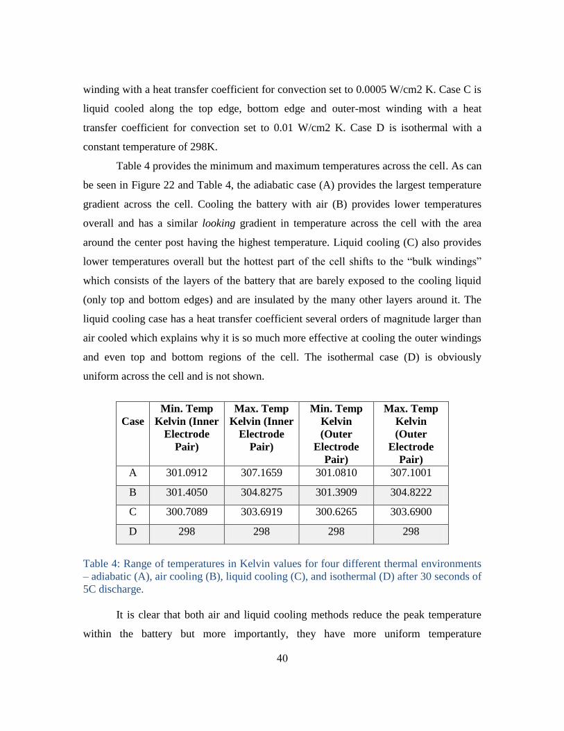
Table 4 provides the minimum and maximum temperatures across the cell. As can

be seen in Figure 22 and Table 4, the adiabatic case (A) provides the largest temperature

gradient across the cell. Cooling the battery with air (B) provides lower temperatures

overall and has a similar looking gradient in temperature across the cell with the area

around the center post having the highest temperature. Liquid cooling (C) also provides

lower temperatures overall but the hottest part of the cell shifts to the “bulk windings”

which consists of the layers of the battery that are barely exposed to the cooling liquid

(only top and bottom edges) and are insulated by the many other layers around it. The

liquid cooling case has a heat transfer coefficient several orders of magnitude larger than

air cooled which explains why it is so much more effective at cooling the outer windings

and even top and bottom regions of the cell. The isothermal case (D) is obviously

uniform across the cell and is not shown.

Case

Min. Temp

Kelvin (Inner

Electrode

Pair)

Max. Temp

Kelvin (Inner

Electrode

Pair)

Min. Temp

Kelvin

(Outer

Electrode

Pair)

Max. Temp

Kelvin

(Outer

Electrode

Pair)

A 301.0912 307.1659 301.0810 307.1001

B 301.4050 304.8275 301.3909 304.8222

C 300.7089 303.6919 300.6265 303.6900

D 298 298 298 298

Table 4: Range of temperatures in Kelvin values for four different thermal environments

– adiabatic (A), air cooling (B), liquid cooling (C), and isothermal (D) after 30 seconds of

5C discharge.

It is clear that both air and liquid cooling methods reduce the peak temperature

within the battery but more importantly, they have more uniform temperature

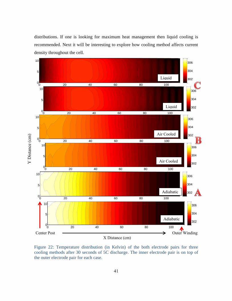
41

distributions. If one is looking for maximum heat management then liquid cooling is

recommended. Next it will be interesting to explore how cooling method affects current

density throughout the cell.

Figure 22: Temperature distribution (in Kelvin) of the both electrode pairs for three

cooling methods after 30 seconds of 5C discharge. The inner electrode pair is on top of

the outer electrode pair for each case.

0 20 40 60 80 1000

5

10

302

304

306

0 20 40 60 80 1000

5

10

302

304

306

0 20 40 60 80 1000

5

10

302

304

306

0 20 40 60 80 1000

5

10

302

304

306

0 20 40 60 80 1000

5

10

302

304

306

0 20 40 60 80 1000

5

10

302

304

306

Center Post Outer Winding

X Distance (cm)

Y D

ista

nce

(cm

)

Adiabatic

Adiabatic

Air Cooled

Air Cooled

Liquid

Cooled

Liquid

Cooled

42

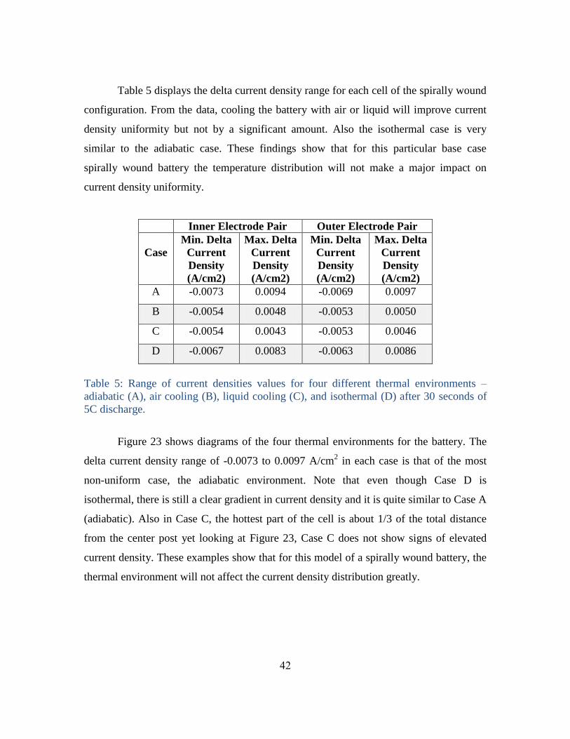
Table 5 displays the delta current density range for each cell of the spirally wound

configuration. From the data, cooling the battery with air or liquid will improve current

density uniformity but not by a significant amount. Also the isothermal case is very

similar to the adiabatic case. These findings show that for this particular base case

spirally wound battery the temperature distribution will not make a major impact on

current density uniformity.

Inner Electrode Pair Outer Electrode Pair

Case

Min. Delta

Current

Density

(A/cm2)

Max. Delta

Current

Density

(A/cm2)

Min. Delta

Current

Density

(A/cm2)

Max. Delta

Current

Density

(A/cm2)

A -0.0073 0.0094 -0.0069 0.0097

B -0.0054 0.0048 -0.0053 0.0050

C -0.0054 0.0043 -0.0053 0.0046

D -0.0067 0.0083 -0.0063 0.0086

Table 5: Range of current densities values for four different thermal environments –

adiabatic (A), air cooling (B), liquid cooling (C), and isothermal (D) after 30 seconds of

5C discharge.

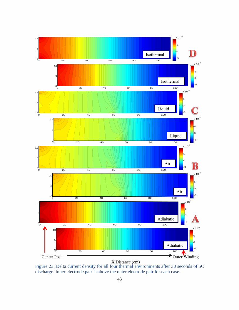
Figure 23 shows diagrams of the four thermal environments for the battery. The

delta current density range of -0.0073 to 0.0097 A/cm2 in each case is that of the most

non-uniform case, the adiabatic environment. Note that even though Case D is

isothermal, there is still a clear gradient in current density and it is quite similar to Case A

(adiabatic). Also in Case C, the hottest part of the cell is about 1/3 of the total distance

from the center post yet looking at Figure 23, Case C does not show signs of elevated

current density. These examples show that for this model of a spirally wound battery, the

thermal environment will not affect the current density distribution greatly.

43

Center Post Outer Winding

X Distance (cm)

Figure 23: Delta current density for all four thermal environments after 30 seconds of 5C

discharge. Inner electrode pair is above the outer electrode pair for each case.

0 20 40 60 80 1000

5

10

-5

0

5

x 10-3

0 20 40 60 80 1000

5

10

-5

0

5

x 10-3

0 20 40 60 80 1000

5

10

-5

0

5

x 10-3

0 20 40 60 80 1000

5

10

-5

0

5

x 10-3

0 20 40 60 80 1000

5

10

-5

0

5

x 10-3

0 20 40 60 80 1000

5

10

-5

0

5

x 10-3

0 20 40 60 80 1000

5

10

-5

0

5

x 10-3

0 20 40 60 80 1000

5

10

-5

0

5

x 10-3

Adiabatic

Adiabatic

Air

Co

Air

Coo

Liquid

Cooled

Liquid

Cooled

Isothermal

Isothermal

44

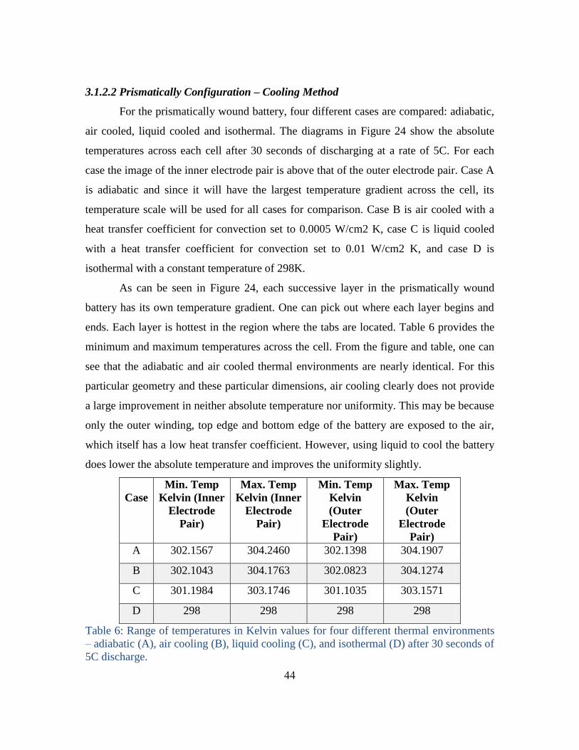
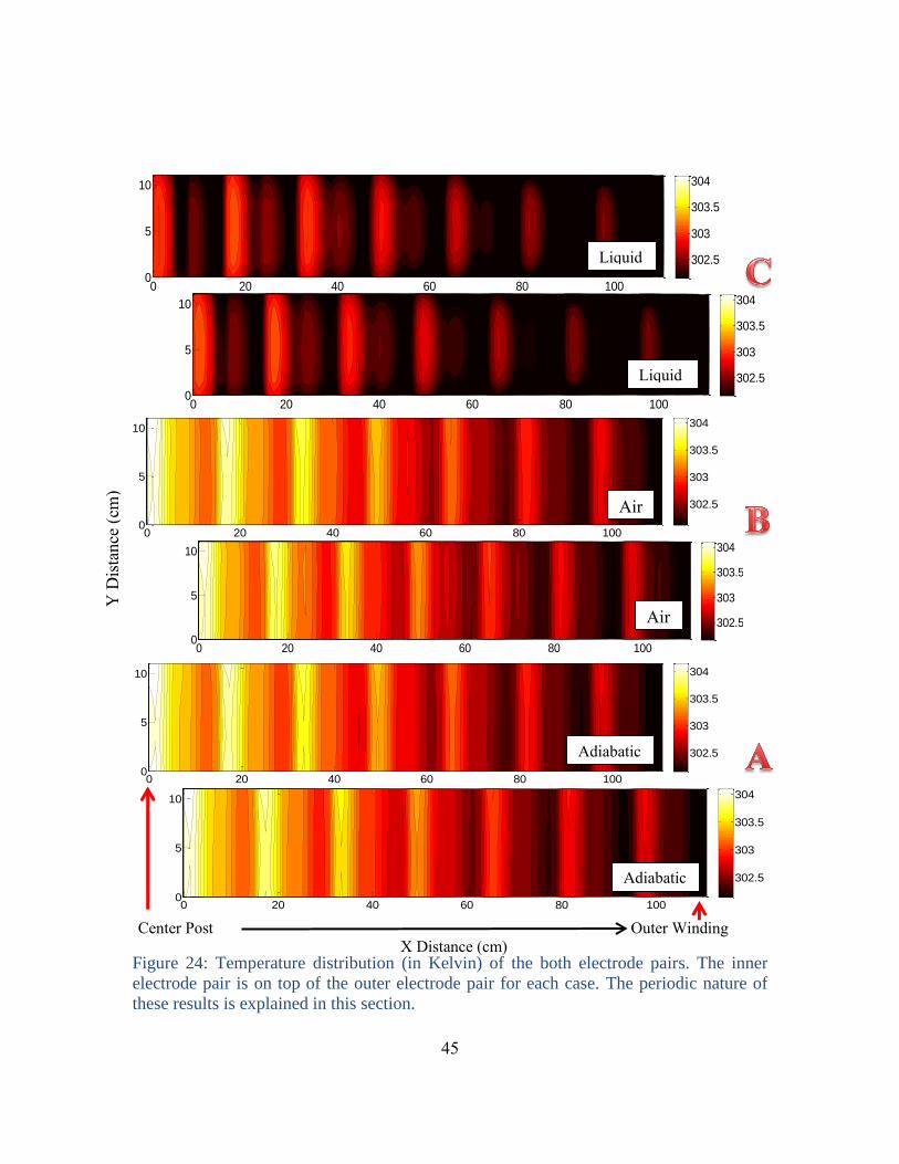
3.1.2.2 Prismatically Configuration – Cooling Method

For the prismatically wound battery, four different cases are compared: adiabatic,

air cooled, liquid cooled and isothermal. The diagrams in Figure 24 show the absolute

temperatures across each cell after 30 seconds of discharging at a rate of 5C. For each

case the image of the inner electrode pair is above that of the outer electrode pair. Case A

is adiabatic and since it will have the largest temperature gradient across the cell, its

temperature scale will be used for all cases for comparison. Case B is air cooled with a

heat transfer coefficient for convection set to 0.0005 W/cm2 K, case C is liquid cooled

with a heat transfer coefficient for convection set to 0.01 W/cm2 K, and case D is

isothermal with a constant temperature of 298K.

As can be seen in Figure 24, each successive layer in the prismatically wound

battery has its own temperature gradient. One can pick out where each layer begins and

ends. Each layer is hottest in the region where the tabs are located. Table 6 provides the

minimum and maximum temperatures across the cell. From the figure and table, one can

see that the adiabatic and air cooled thermal environments are nearly identical. For this

particular geometry and these particular dimensions, air cooling clearly does not provide

a large improvement in neither absolute temperature nor uniformity. This may be because

only the outer winding, top edge and bottom edge of the battery are exposed to the air,

which itself has a low heat transfer coefficient. However, using liquid to cool the battery

does lower the absolute temperature and improves the uniformity slightly.

Case

Min. Temp

Kelvin (Inner

Electrode

Pair)

Max. Temp

Kelvin (Inner

Electrode

Pair)

Min. Temp

Kelvin

(Outer

Electrode

Pair)

Max. Temp

Kelvin

(Outer

Electrode

Pair)

A 302.1567 304.2460 302.1398 304.1907

B 302.1043 304.1763 302.0823 304.1274

C 301.1984 303.1746 301.1035 303.1571

D 298 298 298 298

Table 6: Range of temperatures in Kelvin values for four different thermal environments

– adiabatic (A), air cooling (B), liquid cooling (C), and isothermal (D) after 30 seconds of

5C discharge.

45

Center Post Outer Winding

X Distance (cm)

Figure 24: Temperature distribution (in Kelvin) of the both electrode pairs. The inner

electrode pair is on top of the outer electrode pair for each case. The periodic nature of

these results is explained in this section.

0 20 40 60 80 1000

5

10

302.5

303

303.5

304

0 20 40 60 80 1000

5

10

302.5

303

303.5

304

0 20 40 60 80 1000

5

10

302.5

303

303.5

304

0 20 40 60 80 1000

5

10

302.5

303

303.5

304

0 20 40 60 80 1000

5

10

302.5

303

303.5

304

0 20 40 60 80 1000

5

10

302.5

303

303.5

304

Y D

ista

nce

(cm

)

Adiabatic

Adiabatic

Air

Co

Air

Co

Liquid

Coole

Liquid Coole

46

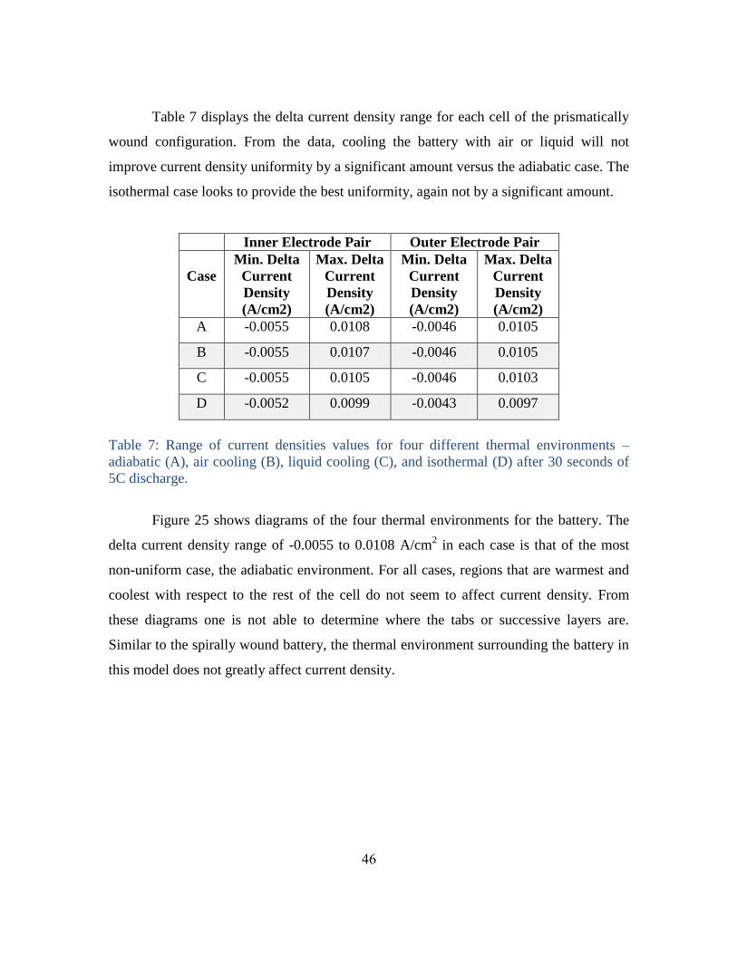
Table 7 displays the delta current density range for each cell of the prismatically

wound configuration. From the data, cooling the battery with air or liquid will not

improve current density uniformity by a significant amount versus the adiabatic case. The

isothermal case looks to provide the best uniformity, again not by a significant amount.

Inner Electrode Pair Outer Electrode Pair

Case

Min. Delta

Current

Density

(A/cm2)

Max. Delta

Current

Density

(A/cm2)

Min. Delta

Current

Density

(A/cm2)

Max. Delta

Current

Density

(A/cm2)

A -0.0055 0.0108 -0.0046 0.0105

B -0.0055 0.0107 -0.0046 0.0105

C -0.0055 0.0105 -0.0046 0.0103

D -0.0052 0.0099 -0.0043 0.0097

Table 7: Range of current densities values for four different thermal environments –

adiabatic (A), air cooling (B), liquid cooling (C), and isothermal (D) after 30 seconds of

5C discharge.

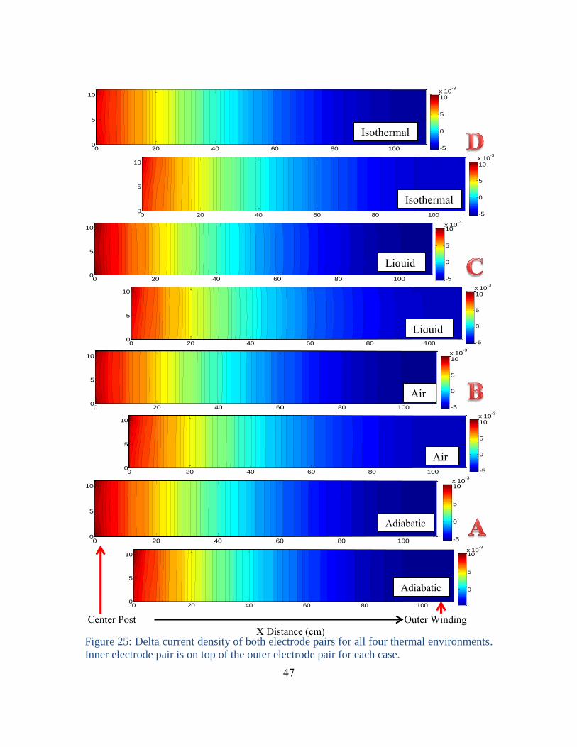
Figure 25 shows diagrams of the four thermal environments for the battery. The

delta current density range of -0.0055 to 0.0108 A/cm2 in each case is that of the most

non-uniform case, the adiabatic environment. For all cases, regions that are warmest and

coolest with respect to the rest of the cell do not seem to affect current density. From

these diagrams one is not able to determine where the tabs or successive layers are.

Similar to the spirally wound battery, the thermal environment surrounding the battery in

this model does not greatly affect current density.

47

Center Post Outer Winding

X Distance (cm)

Figure 25: Delta current density of both electrode pairs for all four thermal environments.

Inner electrode pair is on top of the outer electrode pair for each case.

0 20 40 60 80 1000

5

10

-5

0

5

10x 10

-3

0 20 40 60 80 1000

5

10

-5

0

5

10x 10

-3

0 20 40 60 80 1000

5

10

-5

0

5

10x 10

-3

0 20 40 60 80 1000

5

10

-5

0

5

10x 10

-3

0 20 40 60 80 1000

5

10

-5

0

5

10x 10

-3

0 20 40 60 80 1000

5

10

-5

0

5

10x 10

-3

0 20 40 60 80 1000

5

10

-5

0

5

10x 10

-3

0 20 40 60 80 1000

5

10

0

5

10x 10

-3

Adiabatic

Adiabatic

Air

Coo

Air

Co

Liquid

Cooled

Liquid

Cooled

Isothermal

Isothermal

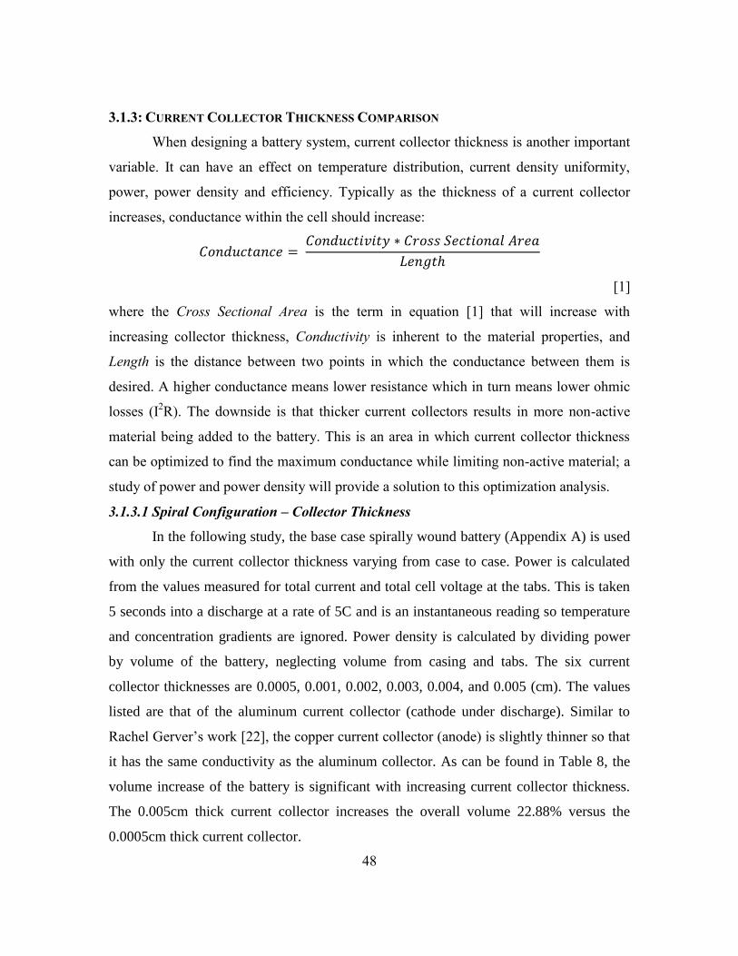
48

3.1.3: CURRENT COLLECTOR THICKNESS COMPARISON

When designing a battery system, current collector thickness is another important

variable. It can have an effect on temperature distribution, current density uniformity,

power, power density and efficiency. Typically as the thickness of a current collector

increases, conductance within the cell should increase:

[1]

where the Cross Sectional Area is the term in equation [1] that will increase with

increasing collector thickness, Conductivity is inherent to the material properties, and

Length is the distance between two points in which the conductance between them is

desired. A higher conductance means lower resistance which in turn means lower ohmic

losses (I2R). The downside is that thicker current collectors results in more non-active

material being added to the battery. This is an area in which current collector thickness

can be optimized to find the maximum conductance while limiting non-active material; a

study of power and power density will provide a solution to this optimization analysis.

3.1.3.1 Spiral Configuration – Collector Thickness

In the following study, the base case spirally wound battery (Appendix A) is used

with only the current collector thickness varying from case to case. Power is calculated

from the values measured for total current and total cell voltage at the tabs. This is taken

5 seconds into a discharge at a rate of 5C and is an instantaneous reading so temperature

and concentration gradients are ignored. Power density is calculated by dividing power

by volume of the battery, neglecting volume from casing and tabs. The six current

collector thicknesses are 0.0005, 0.001, 0.002, 0.003, 0.004, and 0.005 (cm). The values

listed are that of the aluminum current collector (cathode under discharge). Similar to

Rachel Gerver’s work [22], the copper current collector (anode) is slightly thinner so that

it has the same conductivity as the aluminum collector. As can be found in Table 8, the

volume increase of the battery is significant with increasing current collector thickness.

The 0.005cm thick current collector increases the overall volume 22.88% versus the

0.0005cm thick current collector.

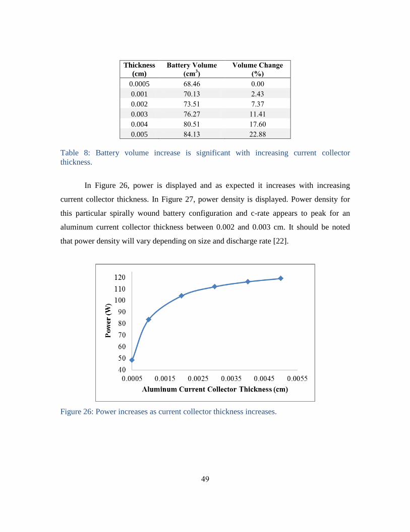
49

Thickness

(cm)

Battery Volume

(cm3)

Volume Change

(%)

0.0005 68.46 0.00

0.001 70.13 2.43

0.002 73.51 7.37

0.003 76.27 11.41

0.004 80.51 17.60

0.005 84.13 22.88

Table 8: Battery volume increase is significant with increasing current collector

thickness.

In Figure 26, power is displayed and as expected it increases with increasing

current collector thickness. In Figure 27, power density is displayed. Power density for

this particular spirally wound battery configuration and c-rate appears to peak for an

aluminum current collector thickness between 0.002 and 0.003 cm. It should be noted

that power density will vary depending on size and discharge rate [22].

Figure 26: Power increases as current collector thickness increases.

50

Figure 27: Power density versus aluminum current collector thickness (cathode under

discharge).

Current collector thickness also affects current density uniformity since

conductance increases with increasing current collector thickness. Results for the six

current collector thicknesses can be found in Figure 28 and Table 9. Figure 28 shows the

difference between current density for each location within the cell and average current

density (ΔI I_x,y – I_avg). Since tab locations and cooling method are the same for all

cases, only the inner electrode pair current densities are displayed. Table 9 shows the

delta current density range of each case.

As one might expect, the current density across the cell becomes more uniform as

the current collector thickness increases. When looking at all three figures, particularly

Figure 28, and the values from Table 9, an aluminum current collector thickness from

0.002 – 0.003cm may be best for optimizing power, power density, and current density

uniformity for this particular spirally wound configuration discharging at a 5C rate.

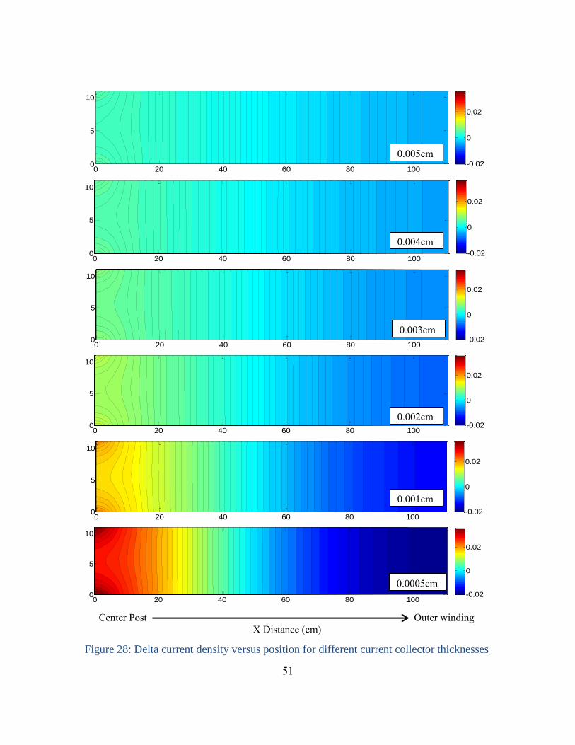
51

Figure 28: Delta current density versus position for different current collector thicknesses

0 20 40 60 80 1000

5

10

-0.02

0

0.02

0 20 40 60 80 1000

5

10

-0.02

0

0.02

0 20 40 60 80 1000

5

10

-0.02

0

0.02

0 20 40 60 80 1000

5

10

-0.02

0

0.02

0 20 40 60 80 1000

5

10

-0.02

0

0.02

0 20 40 60 80 1000

5

10

-0.02

0

0.02

Center Post Outer winding

X Distance (cm)

0.0005cm

0.001cm

0.002cm

0.003cm

0.004cm

0.005cm

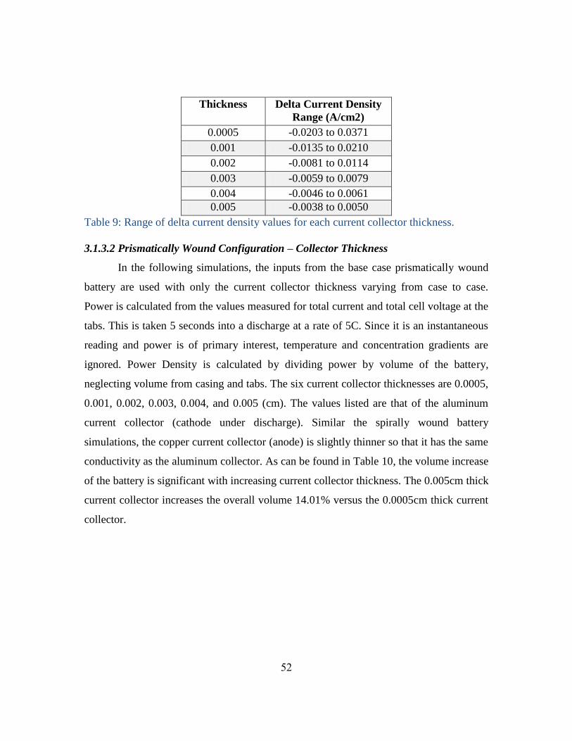
52

Thickness

Delta Current Density

Range (A/cm2)

0.0005 -0.0203 to 0.0371

0.001 -0.0135 to 0.0210

0.002 -0.0081 to 0.0114

0.003 -0.0059 to 0.0079

0.004 -0.0046 to 0.0061

0.005 -0.0038 to 0.0050

Table 9: Range of delta current density values for each current collector thickness.

3.1.3.2 Prismatically Wound Configuration – Collector Thickness

In the following simulations, the inputs from the base case prismatically wound

battery are used with only the current collector thickness varying from case to case.

Power is calculated from the values measured for total current and total cell voltage at the

tabs. This is taken 5 seconds into a discharge at a rate of 5C. Since it is an instantaneous

reading and power is of primary interest, temperature and concentration gradients are

ignored. Power Density is calculated by dividing power by volume of the battery,

neglecting volume from casing and tabs. The six current collector thicknesses are 0.0005,

0.001, 0.002, 0.003, 0.004, and 0.005 (cm). The values listed are that of the aluminum

current collector (cathode under discharge). Similar the spirally wound battery

simulations, the copper current collector (anode) is slightly thinner so that it has the same

conductivity as the aluminum collector. As can be found in Table 10, the volume increase

of the battery is significant with increasing current collector thickness. The 0.005cm thick

current collector increases the overall volume 14.01% versus the 0.0005cm thick current

collector.

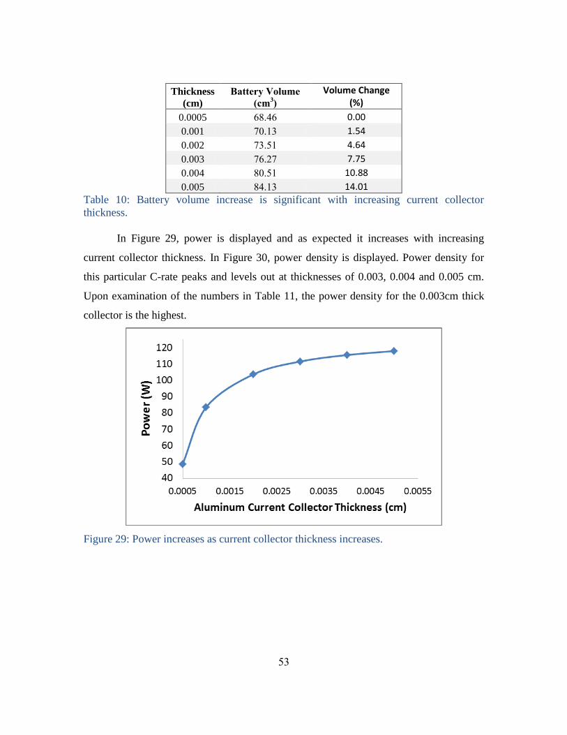
53

Thickness

(cm)

Battery Volume

(cm3)

Volume Change (%)

0.0005 68.46 0.00

0.001 70.13 1.54

0.002 73.51 4.64

0.003 76.27 7.75

0.004 80.51 10.88

0.005 84.13 14.01

Table 10: Battery volume increase is significant with increasing current collector

thickness.

In Figure 29, power is displayed and as expected it increases with increasing

current collector thickness. In Figure 30, power density is displayed. Power density for

this particular C-rate peaks and levels out at thicknesses of 0.003, 0.004 and 0.005 cm.

Upon examination of the numbers in Table 11, the power density for the 0.003cm thick

collector is the highest.

Figure 29: Power increases as current collector thickness increases.

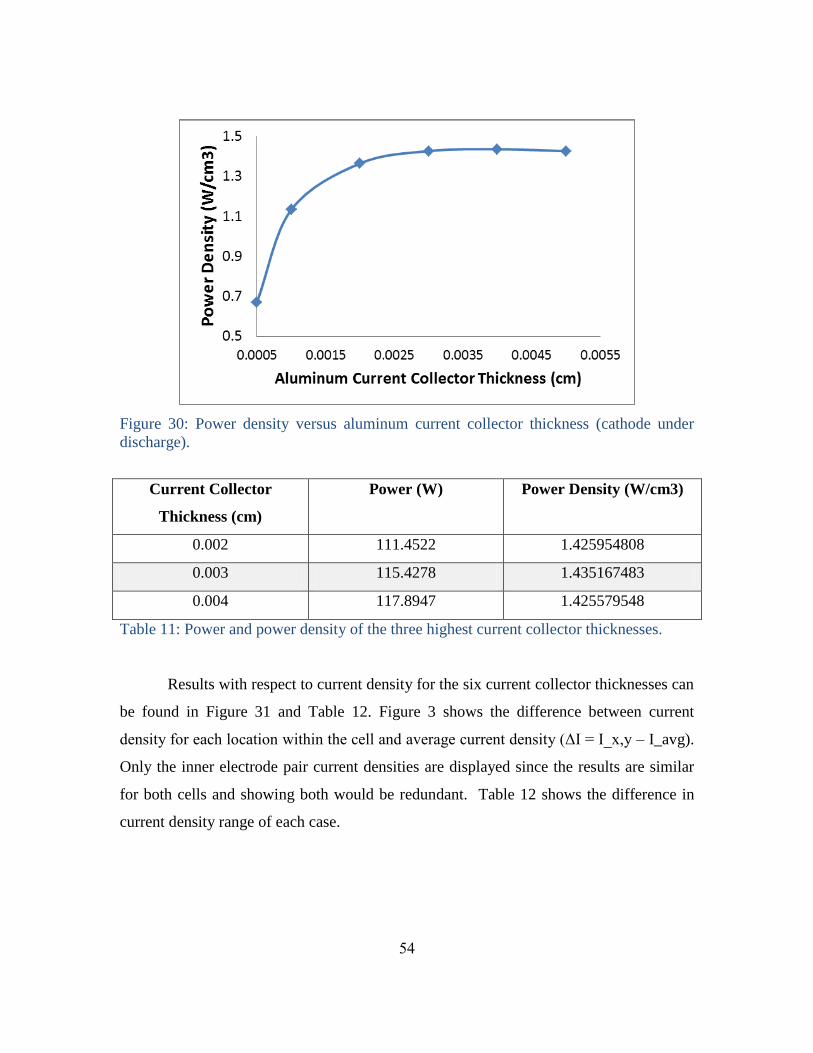
54

Figure 30: Power density versus aluminum current collector thickness (cathode under

discharge).

Current Collector

Thickness (cm)

Power (W) Power Density (W/cm3)

0.002 111.4522 1.425954808

0.003 115.4278 1.435167483

0.004 117.8947 1.425579548

Table 11: Power and power density of the three highest current collector thicknesses.

Results with respect to current density for the six current collector thicknesses can

be found in Figure 31 and Table 12. Figure 3 shows the difference between current

density for each location within the cell and average current density (ΔI I_x,y – I_avg).

Only the inner electrode pair current densities are displayed since the results are similar

for both cells and showing both would be redundant. Table 12 shows the difference in

current density range of each case.

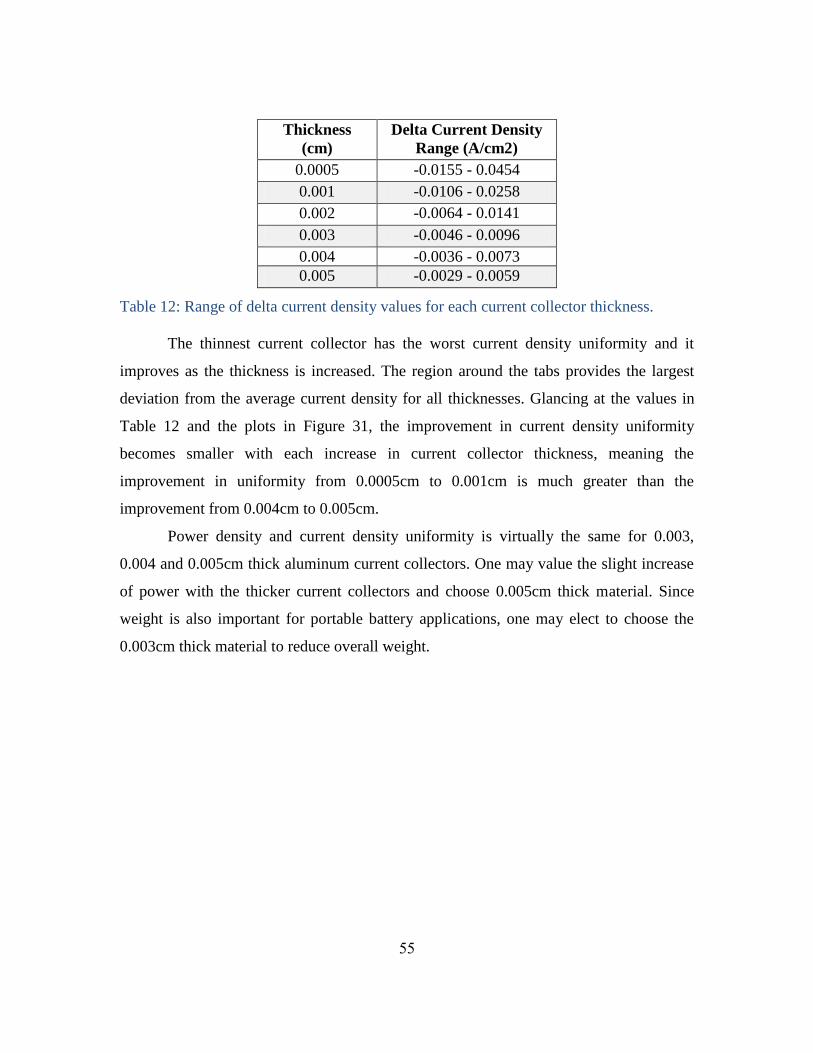
55

Thickness

(cm)

Delta Current Density

Range (A/cm2)

0.0005 -0.0155 - 0.0454

0.001 -0.0106 - 0.0258

0.002 -0.0064 - 0.0141

0.003 -0.0046 - 0.0096

0.004 -0.0036 - 0.0073

0.005 -0.0029 - 0.0059

Table 12: Range of delta current density values for each current collector thickness.

The thinnest current collector has the worst current density uniformity and it

improves as the thickness is increased. The region around the tabs provides the largest

deviation from the average current density for all thicknesses. Glancing at the values in

Table 12 and the plots in Figure 31, the improvement in current density uniformity

becomes smaller with each increase in current collector thickness, meaning the

improvement in uniformity from 0.0005cm to 0.001cm is much greater than the

improvement from 0.004cm to 0.005cm.

Power density and current density uniformity is virtually the same for 0.003,

0.004 and 0.005cm thick aluminum current collectors. One may value the slight increase

of power with the thicker current collectors and choose 0.005cm thick material. Since

weight is also important for portable battery applications, one may elect to choose the

0.003cm thick material to reduce overall weight.

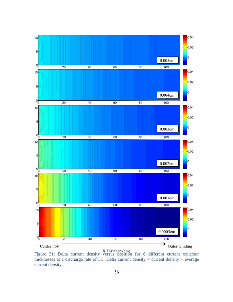
56

Center Post Outer winding

X Distance (cm)

Figure 31: Delta current density versus position for 6 different current collector

thicknesses at a discharge rate of 5C. Delta current density = current density – average

current density.

0 20 40 60 80 1000

5

10

0

0.02

0.04

0 20 40 60 80 1000

5

10

0

0.02

0.04

0 20 40 60 80 1000

5

10

0

0.02

0.04

0 20 40 60 80 1000

5

10

0

0.02

0.04

0 20 40 60 80 1000

5

10

0

0.02

0.04

0 20 40 60 80 1000

5

10

0

0.02

0.04

0.0005cm

0.001cm

0.002cm

0.003cm

0.004cm

0.005cm

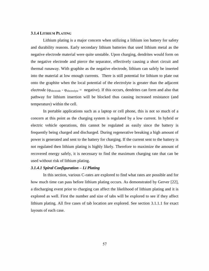
57

3.1.4 LITHIUM PLATING

Lithium plating is a major concern when utilizing a lithium ion battery for safety

and durability reasons. Early secondary lithium batteries that used lithium metal as the

negative electrode material were quite unstable. Upon charging, dendrites would form on

the negative electrode and pierce the separator, effectively causing a short circuit and

thermal runaway. With graphite as the negative electrode, lithium can safely be inserted

into the material at low enough currents. There is still potential for lithium to plate out

onto the graphite when the local potential of the electrolyte is greater than the adjacent

electrode (φelectrode - φelectrolyte = negative). If this occurs, dendrites can form and also that

pathway for lithium insertion will be blocked thus causing increased resistance (and

temperature) within the cell.

In portable applications such as a laptop or cell phone, this is not so much of a

concern at this point as the charging system is regulated by a low current. In hybrid or

electric vehicle operations, this cannot be regulated as easily since the battery is

frequently being charged and discharged. During regenerative breaking a high amount of

power is generated and sent to the battery for charging. If the current sent to the battery is

not regulated then lithium plating is highly likely. Therefore to maximize the amount of

recovered energy safely, it is necessary to find the maximum charging rate that can be

used without risk of lithium plating.

3.1.4.1 Spiral Configuration – Li Plating

In this section, various C-rates are explored to find what rates are possible and for

how much time can pass before lithium plating occurs. As demonstrated by Gerver [22],

a discharging event prior to charging can affect the likelihood of lithium plating and it is

explored as well. First the number and size of tabs will be explored to see if they affect

lithium plating. All five cases of tab location are explored. See section 3.1.1.1 for exact

layouts of each case.

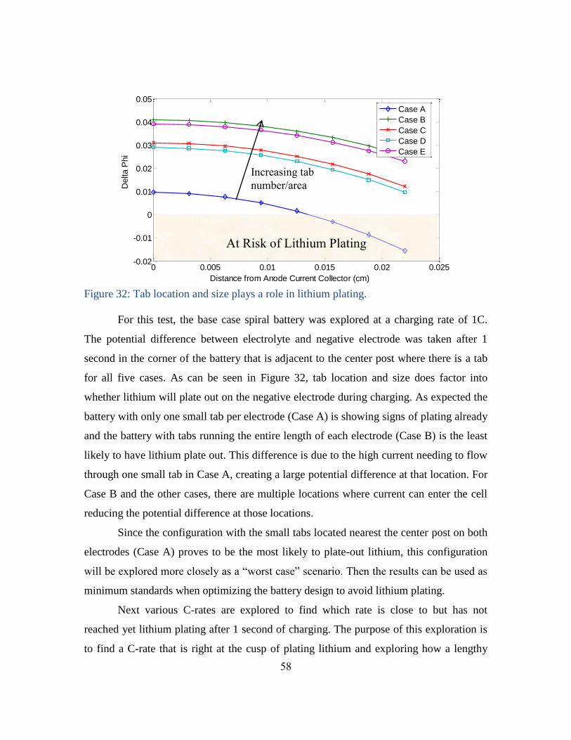
58

Figure 32: Tab location and size plays a role in lithium plating.

For this test, the base case spiral battery was explored at a charging rate of 1C.

The potential difference between electrolyte and negative electrode was taken after 1

second in the corner of the battery that is adjacent to the center post where there is a tab

for all five cases. As can be seen in Figure 32, tab location and size does factor into

whether lithium will plate out on the negative electrode during charging. As expected the

battery with only one small tab per electrode (Case A) is showing signs of plating already

and the battery with tabs running the entire length of each electrode (Case B) is the least

likely to have lithium plate out. This difference is due to the high current needing to flow

through one small tab in Case A, creating a large potential difference at that location. For

Case B and the other cases, there are multiple locations where current can enter the cell

reducing the potential difference at those locations.

Since the configuration with the small tabs located nearest the center post on both

electrodes (Case A) proves to be the most likely to plate-out lithium, this configuration

will be explored more closely as a “worst case” scenario. Then the results can be used as

minimum standards when optimizing the battery design to avoid lithium plating.

Next various C-rates are explored to find which rate is close to but has not

reached yet lithium plating after 1 second of charging. The purpose of this exploration is

to find a C-rate that is right at the cusp of plating lithium and exploring how a lengthy

0 0.005 0.01 0.015 0.02 0.025-0.02

-0.01

0

0.01

0.02

0.03

0.04

0.05

Distance from Anode Current Collector (cm)

Delta P

hi

Lithium Plating with respect to Tab Location

Case A

Case B

Case C

Case D

Case E

Increasing tab

number/area

At Risk of Lithium Plating

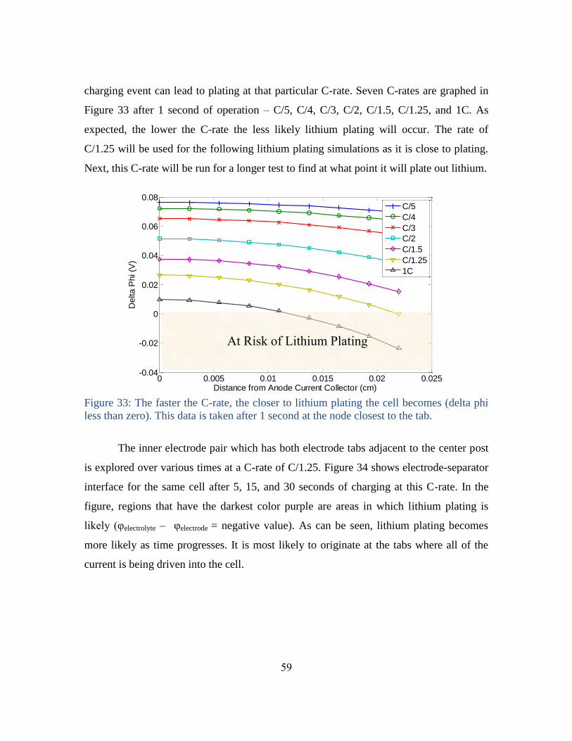
59

charging event can lead to plating at that particular C-rate. Seven C-rates are graphed in

Figure 33 after 1 second of operation – C/5, C/4, C/3, C/2, C/1.5, C/1.25, and 1C. As

expected, the lower the C-rate the less likely lithium plating will occur. The rate of

C/1.25 will be used for the following lithium plating simulations as it is close to plating.

Next, this C-rate will be run for a longer test to find at what point it will plate out lithium.

Figure 33: The faster the C-rate, the closer to lithium plating the cell becomes (delta phi

less than zero). This data is taken after 1 second at the node closest to the tab.

The inner electrode pair which has both electrode tabs adjacent to the center post

is explored over various times at a C-rate of C/1.25. Figure 34 shows electrode-separator

interface for the same cell after 5, 15, and 30 seconds of charging at this C-rate. In the

figure, regions that have the darkest color purple are areas in which lithium plating is

likely (φelectrolyte – φelectrode = negative value). As can be seen, lithium plating becomes

more likely as time progresses. It is most likely to originate at the tabs where all of the

current is being driven into the cell.

0 0.005 0.01 0.015 0.02 0.025-0.04

-0.02

0

0.02

0.04

0.06

0.08

Distance from Anode Current Collector (cm)

Delta P

hi (V

)

Lithium Plating with respect to C - rate

C/5

C/4

C/3

C/2

C/1.5

C/1.25

1C

At Risk of Lithium Plating

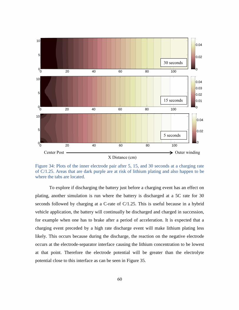
60

Figure 34: Plots of the inner electrode pair after 5, 15, and 30 seconds at a charging rate

of C/1.25. Areas that are dark purple are at risk of lithium plating and also happen to be

where the tabs are located.

To explore if discharging the battery just before a charging event has an effect on

plating, another simulation is run where the battery is discharged at a 5C rate for 30

seconds followed by charging at a C-rate of C/1.25. This is useful because in a hybrid

vehicle application, the battery will continually be discharged and charged in succession,

for example when one has to brake after a period of acceleration. It is expected that a

charging event preceded by a high rate discharge event will make lithium plating less

likely. This occurs because during the discharge, the reaction on the negative electrode

occurs at the electrode-separator interface causing the lithium concentration to be lowest

at that point. Therefore the electrode potential will be greater than the electrolyte

potential close to this interface as can be seen in Figure 35.

0 20 40 60 80 1000

5

10

0

0.02

0.04

0 20 40 60 80 1000

5

10

0

0.01

0.02

0.03

0.04

0 20 40 60 80 1000

5

10

0

0.02

0.04

5 seconds

15 seconds

30 seconds

Center Post Outer winding

X Distance (cm)

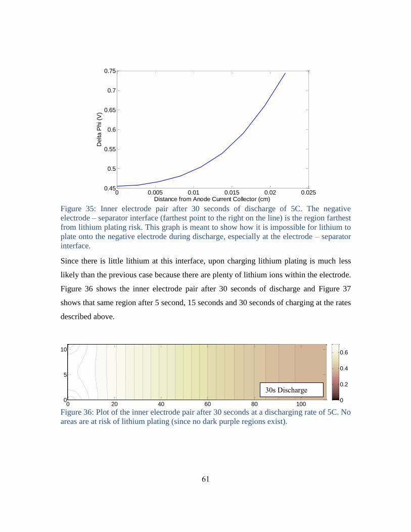
61

Figure 35: Inner electrode pair after 30 seconds of discharge of 5C. The negative

electrode – separator interface (farthest point to the right on the line) is the region farthest

from lithium plating risk. This graph is meant to show how it is impossible for lithium to

plate onto the negative electrode during discharge, especially at the electrode – separator

interface.

Since there is little lithium at this interface, upon charging lithium plating is much less

likely than the previous case because there are plenty of lithium ions within the electrode.

Figure 36 shows the inner electrode pair after 30 seconds of discharge and Figure 37

shows that same region after 5 second, 15 seconds and 30 seconds of charging at the rates

described above.

Figure 36: Plot of the inner electrode pair after 30 seconds at a discharging rate of 5C. No

areas are at risk of lithium plating (since no dark purple regions exist).

0 0.005 0.01 0.015 0.02 0.0250.45

0.5

0.55

0.6

0.65

0.7

0.75

Distance from Anode Current Collector (cm)

Delta P

hi (V

)

Lithium Plating with respect to Discharging

0 20 40 60 80 1000

5

10

0

0.2

0.4

0.6

30s Discharge

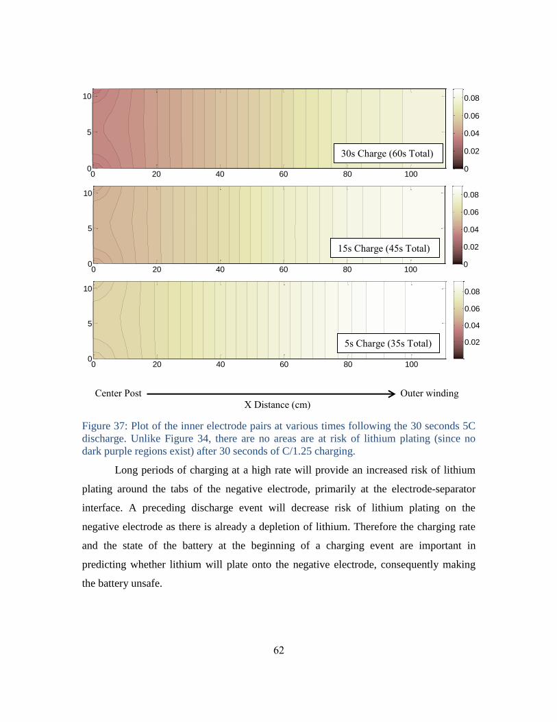
62

Figure 37: Plot of the inner electrode pairs at various times following the 30 seconds 5C

discharge. Unlike Figure 34, there are no areas are at risk of lithium plating (since no

dark purple regions exist) after 30 seconds of C/1.25 charging.

Long periods of charging at a high rate will provide an increased risk of lithium

plating around the tabs of the negative electrode, primarily at the electrode-separator

interface. A preceding discharge event will decrease risk of lithium plating on the

negative electrode as there is already a depletion of lithium. Therefore the charging rate

and the state of the battery at the beginning of a charging event are important in

predicting whether lithium will plate onto the negative electrode, consequently making

the battery unsafe.

0 20 40 60 80 1000

5

10

0

0.02

0.04

0.06

0.08

0 20 40 60 80 1000

5

10

0

0.02

0.04

0.06

0.08

0 20 40 60 80 1000

5

10

0.02

0.04

0.06

0.08

5s Charge (35s Total)

15s Charge (45s Total)

30s Charge (60s Total)

Center Post Outer winding

X Distance (cm)

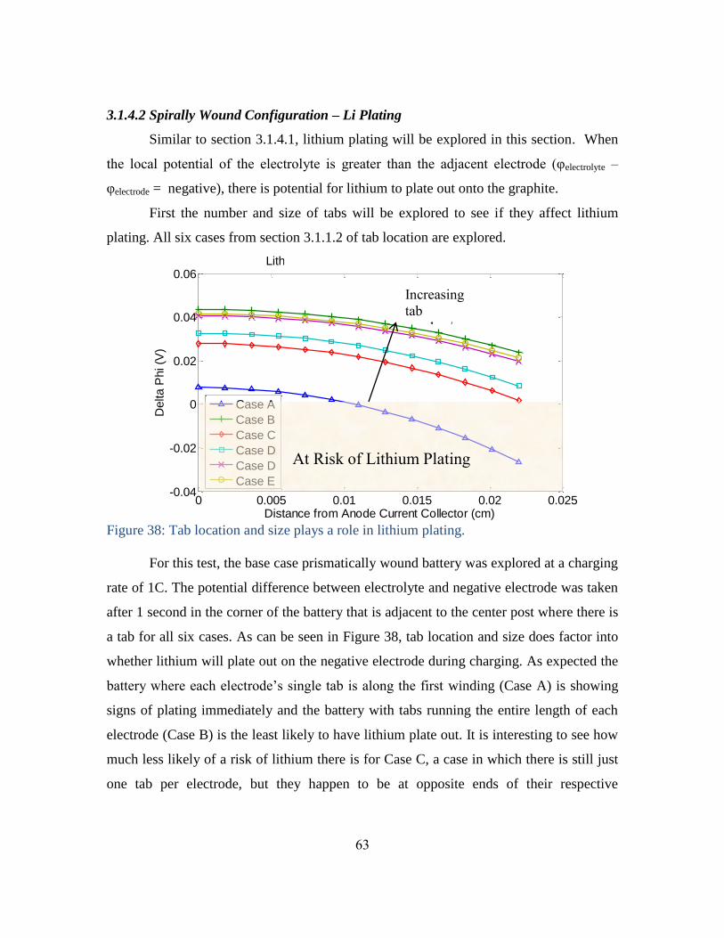
63

3.1.4.2 Spirally Wound Configuration – Li Plating

Similar to section 3.1.4.1, lithium plating will be explored in this section. When

the local potential of the electrolyte is greater than the adjacent electrode (φelectrolyte –

φelectrode = negative), there is potential for lithium to plate out onto the graphite.

First the number and size of tabs will be explored to see if they affect lithium

plating. All six cases from section 3.1.1.2 of tab location are explored.

Figure 38: Tab location and size plays a role in lithium plating.

For this test, the base case prismatically wound battery was explored at a charging

rate of 1C. The potential difference between electrolyte and negative electrode was taken

after 1 second in the corner of the battery that is adjacent to the center post where there is

a tab for all six cases. As can be seen in Figure 38, tab location and size does factor into

whether lithium will plate out on the negative electrode during charging. As expected the

battery where each electrode’s single tab is along the first winding (Case A) is showing

signs of plating immediately and the battery with tabs running the entire length of each

electrode (Case B) is the least likely to have lithium plate out. It is interesting to see how

much less likely of a risk of lithium there is for Case C, a case in which there is still just

one tab per electrode, but they happen to be at opposite ends of their respective

0 0.005 0.01 0.015 0.02 0.025-0.04

-0.02

0

0.02

0.04

0.06

Distance from Anode Current Collector (cm)

Delta P

hi (V

)

Lithium Plating with respect to Tab Location

Case A

Case B

Case C

Case D

Case D

Case E

Increasing

tab

number/area

At Risk of Lithium Plating

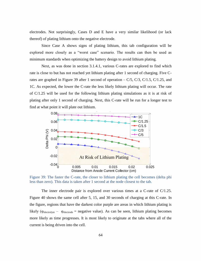
64

electrodes. Not surprisingly, Cases D and E have a very similar likelihood (or lack

thereof) of plating lithium onto the negative electrode.

Since Case A shows signs of plating lithium, this tab configuration will be

explored more closely as a “worst case” scenario. The results can then be used as

minimum standards when optimizing the battery design to avoid lithium plating.

Next, as was done in section 3.1.4.1, various C-rates are explored to find which

rate is close to but has not reached yet lithium plating after 1 second of charging. Five C-

rates are graphed in Figure 39 after 1 second of operation – C/5, C/3, C/1.5, C/1.25, and

1C. As expected, the lower the C-rate the less likely lithium plating will occur. The rate

of C/1.25 will be used for the following lithium plating simulations as it is at risk of

plating after only 1 second of charging. Next, this C-rate will be run for a longer test to

find at what point it will plate out lithium.

Figure 39: The faster the C-rate, the closer to lithium plating the cell becomes (delta phi

less than zero). This data is taken after 1 second at the node closest to the tab.

The inner electrode pair is explored over various times at a C-rate of C/1.25.

Figure 40 shows the same cell after 5, 15, and 30 seconds of charging at this C-rate. In

the figure, regions that have the darkest color purple are areas in which lithium plating is

likely (φelectrolyte – φelectrode = negative value). As can be seen, lithium plating becomes

more likely as time progresses. It is most likely to originate at the tabs where all of the

current is being driven into the cell.

0 0.005 0.01 0.015 0.02 0.025-0.04

-0.02

0

0.02

0.04

0.06

0.08

Distance from Anode Current Collector (cm)

Delta P

hi (V

)

Lithium Plating with respect to C-Rate

1C

C/1.25

C/1.5

C/3

C/5

At Risk of Lithium Plating

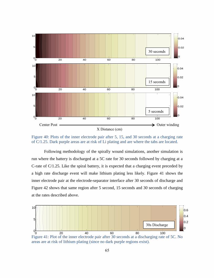
65

Figure 40: Plots of the inner electrode pair after 5, 15, and 30 seconds at a charging rate

of C/1.25. Dark purple areas are at risk of Li plating and are where the tabs are located.

Following methodology of the spirally wound simulations, another simulation is

run where the battery is discharged at a 5C rate for 30 seconds followed by charging at a

C-rate of C/1.25. Like the spiral battery, it is expected that a charging event preceded by

a high rate discharge event will make lithium plating less likely. Figure 41 shows the

inner electrode pair at the electrode-separator interface after 30 seconds of discharge and

Figure 42 shows that same region after 5 second, 15 seconds and 30 seconds of charging

at the rates described above.

Figure 41: Plot of the inner electrode pair after 30 seconds at a discharging rate of 5C. No

areas are at risk of lithium plating (since no dark purple regions exist).

0 20 40 60 80 1000

5

10

0

0.02

0.04

0 20 40 60 80 1000

5

10

0

0.02

0.04

0 20 40 60 80 1000

5

10

0

0.02

0.04

0 20 40 60 80 1000

5

10

0

0.2

0.4

0.6

5 seconds

15 seconds

30 seconds

Center Post Outer winding

X Distance (cm)

30s Discharge

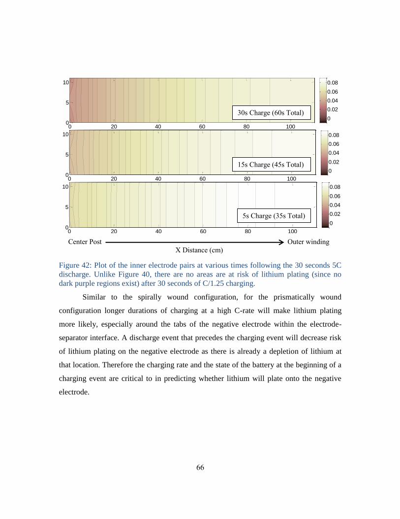
66

Figure 42: Plot of the inner electrode pairs at various times following the 30 seconds 5C

discharge. Unlike Figure 40, there are no areas are at risk of lithium plating (since no

dark purple regions exist) after 30 seconds of C/1.25 charging.

Similar to the spirally wound configuration, for the prismatically wound

configuration longer durations of charging at a high C-rate will make lithium plating

more likely, especially around the tabs of the negative electrode within the electrode-

separator interface. A discharge event that precedes the charging event will decrease risk

of lithium plating on the negative electrode as there is already a depletion of lithium at

that location. Therefore the charging rate and the state of the battery at the beginning of a

charging event are critical to in predicting whether lithium will plate onto the negative

electrode.

0 20 40 60 80 1000

5

10

0

0.02

0.04

0.06

0.08

0 20 40 60 80 1000

5

10

0

0.02

0.04

0.06

0.08

0 20 40 60 80 1000

5

10

0

0.02

0.04

0.06

0.08

5s Charge (35s Total)

15s Charge (45s Total)

30s Charge (60s Total)

Center Post Outer winding

X Distance (cm)

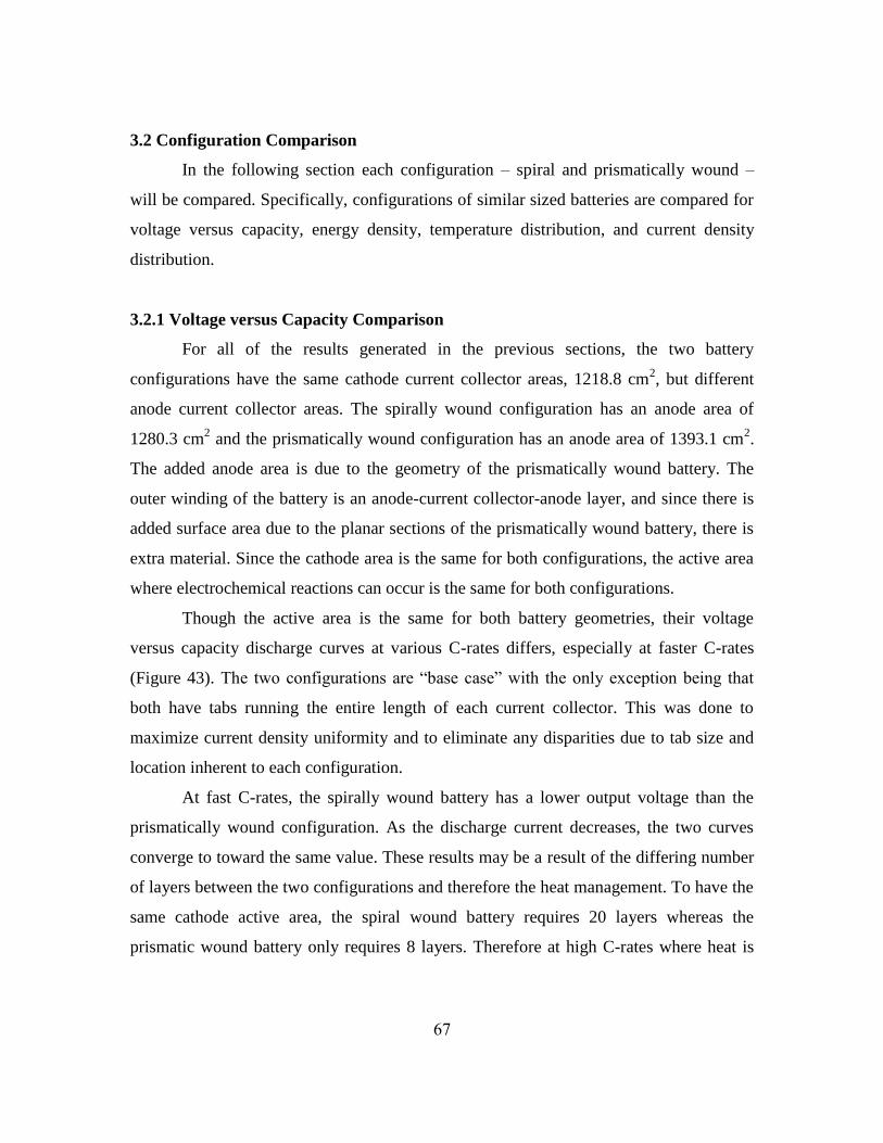
67

3.2 Configuration Comparison

In the following section each configuration – spiral and prismatically wound –

will be compared. Specifically, configurations of similar sized batteries are compared for

voltage versus capacity, energy density, temperature distribution, and current density

distribution.

3.2.1 Voltage versus Capacity Comparison

For all of the results generated in the previous sections, the two battery

configurations have the same cathode current collector areas, 1218.8 cm2, but different

anode current collector areas. The spirally wound configuration has an anode area of

1280.3 cm2 and the prismatically wound configuration has an anode area of 1393.1 cm

2.

The added anode area is due to the geometry of the prismatically wound battery. The

outer winding of the battery is an anode-current collector-anode layer, and since there is

added surface area due to the planar sections of the prismatically wound battery, there is

extra material. Since the cathode area is the same for both configurations, the active area

where electrochemical reactions can occur is the same for both configurations.

Though the active area is the same for both battery geometries, their voltage

versus capacity discharge curves at various C-rates differs, especially at faster C-rates

(Figure 43). The two configurations are “base case” with the only exception being that

both have tabs running the entire length of each current collector. This was done to

maximize current density uniformity and to eliminate any disparities due to tab size and

location inherent to each configuration.

At fast C-rates, the spirally wound battery has a lower output voltage than the

prismatically wound configuration. As the discharge current decreases, the two curves

converge to toward the same value. These results may be a result of the differing number

of layers between the two configurations and therefore the heat management. To have the

same cathode active area, the spiral wound battery requires 20 layers whereas the

prismatic wound battery only requires 8 layers. Therefore at high C-rates where heat is

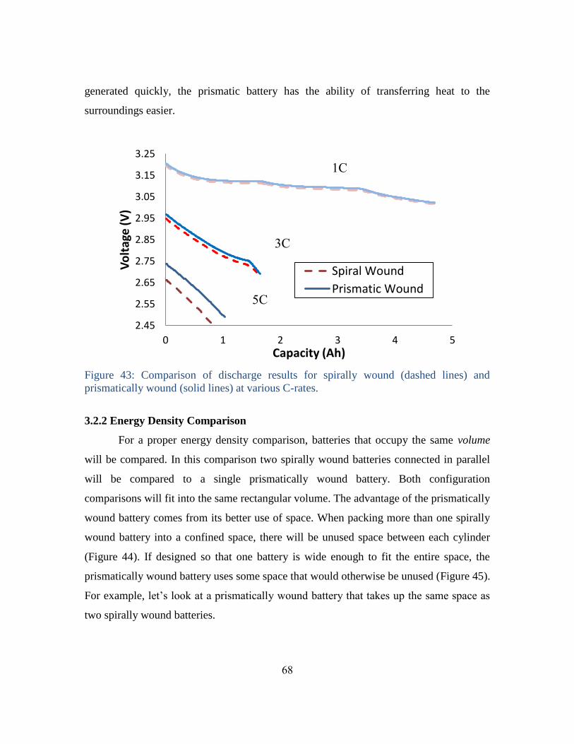
68

generated quickly, the prismatic battery has the ability of transferring heat to the

surroundings easier.

Figure 43: Comparison of discharge results for spirally wound (dashed lines) and

prismatically wound (solid lines) at various C-rates.

3.2.2 Energy Density Comparison

For a proper energy density comparison, batteries that occupy the same volume

will be compared. In this comparison two spirally wound batteries connected in parallel

will be compared to a single prismatically wound battery. Both configuration

comparisons will fit into the same rectangular volume. The advantage of the prismatically

wound battery comes from its better use of space. When packing more than one spirally

wound battery into a confined space, there will be unused space between each cylinder

(Figure 44). If designed so that one battery is wide enough to fit the entire space, the

prismatically wound battery uses some space that would otherwise be unused (Figure 45).

For example, let’s look at a prismatically wound battery that takes up the same space as

two spirally wound batteries.

2.45

2.55

2.65

2.75

2.85

2.95

3.05

3.15

3.25

0 1 2 3 4 5

Vo

ltag

e (

V)

Capacity (Ah)

Spiral Wound

Prismatic Wound

1C

3C

5C

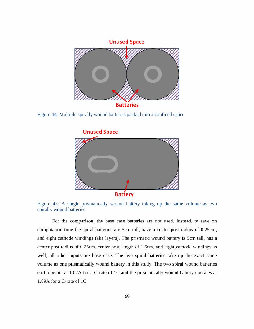
69

Figure 44: Multiple spirally wound batteries packed into a confined space

Figure 45: A single prismatically wound battery taking up the same volume as two

spirally wound batteries

For the comparison, the base case batteries are not used. Instead, to save on

computation time the spiral batteries are 5cm tall, have a center post radius of 0.25cm,

and eight cathode windings (aka layers). The prismatic wound battery is 5cm tall, has a

center post radius of 0.25cm, center post length of 1.5cm, and eight cathode windings as

well; all other inputs are base case. The two spiral batteries take up the exact same

volume as one prismatically wound battery in this study. The two spiral wound batteries

each operate at 1.02A for a C-rate of 1C and the prismatically wound battery operates at

1.89A for a C-rate of 1C.

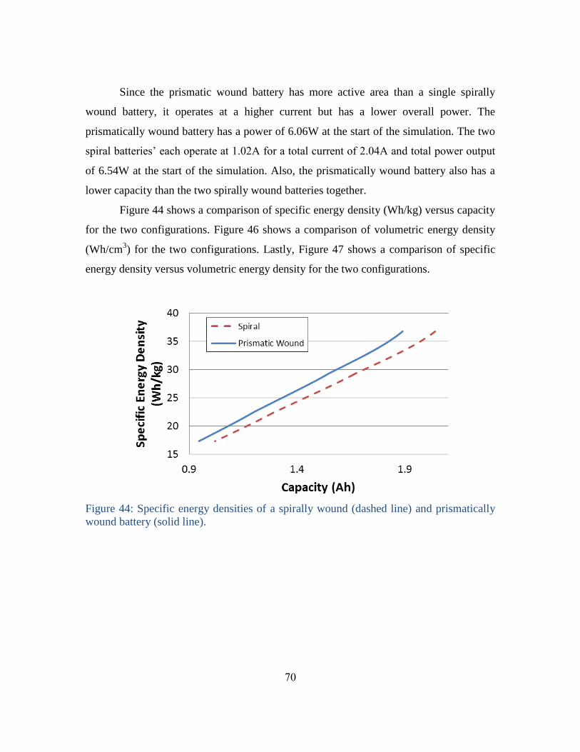
70

Since the prismatic wound battery has more active area than a single spirally

wound battery, it operates at a higher current but has a lower overall power. The

prismatically wound battery has a power of 6.06W at the start of the simulation. The two

spiral batteries’ each operate at 1.02A for a total current of 2.04A and total power output

of 6.54W at the start of the simulation. Also, the prismatically wound battery also has a

lower capacity than the two spirally wound batteries together.

Figure 44 shows a comparison of specific energy density (Wh/kg) versus capacity

for the two configurations. Figure 46 shows a comparison of volumetric energy density

(Wh/cm3) for the two configurations. Lastly, Figure 47 shows a comparison of specific

energy density versus volumetric energy density for the two configurations.

Figure 44: Specific energy densities of a spirally wound (dashed line) and prismatically

wound battery (solid line).

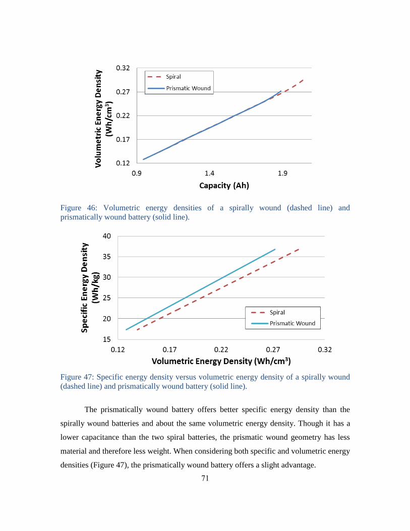
71

Figure 46: Volumetric energy densities of a spirally wound (dashed line) and

prismatically wound battery (solid line).

Figure 47: Specific energy density versus volumetric energy density of a spirally wound

(dashed line) and prismatically wound battery (solid line).

The prismatically wound battery offers better specific energy density than the

spirally wound batteries and about the same volumetric energy density. Though it has a

lower capacitance than the two spiral batteries, the prismatic wound geometry has less

material and therefore less weight. When considering both specific and volumetric energy

densities (Figure 47), the prismatically wound battery offers a slight advantage.

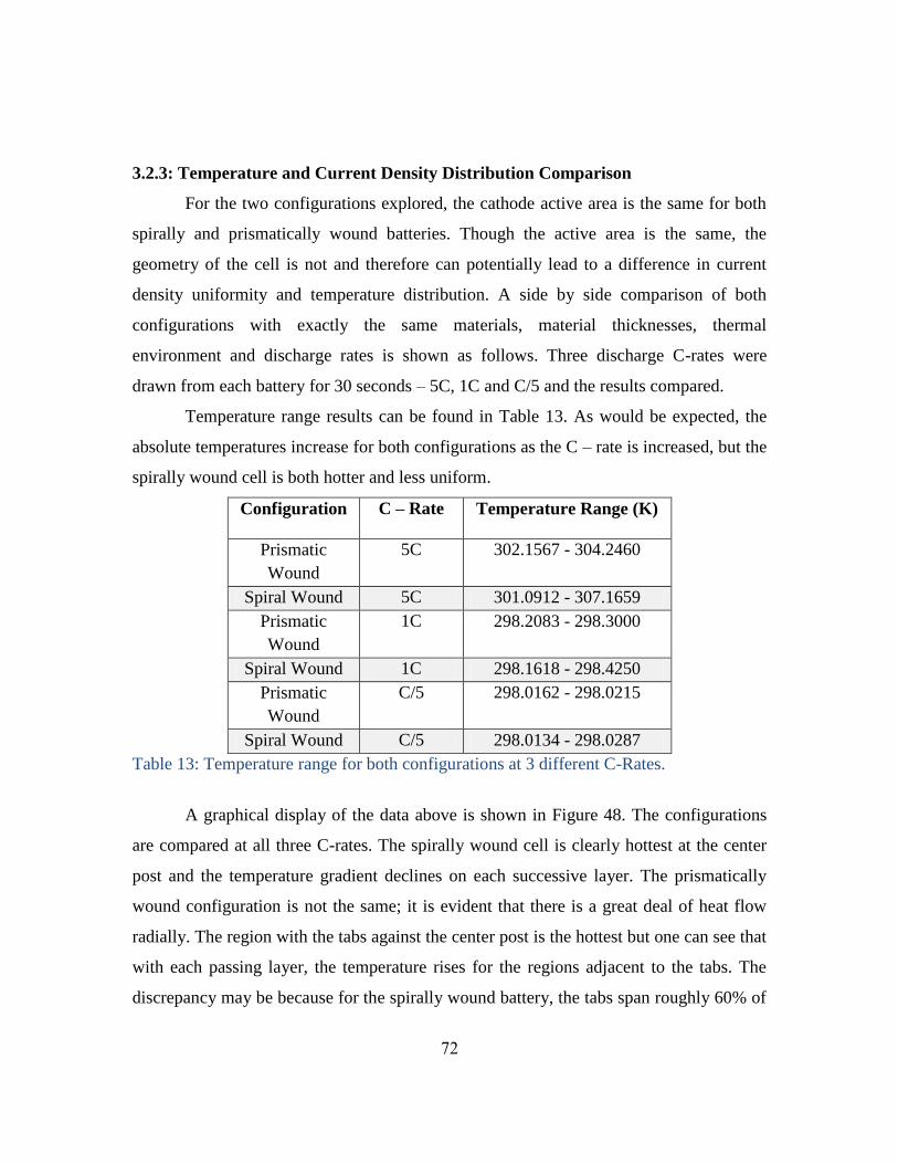
72

3.2.3: Temperature and Current Density Distribution Comparison

For the two configurations explored, the cathode active area is the same for both

spirally and prismatically wound batteries. Though the active area is the same, the

geometry of the cell is not and therefore can potentially lead to a difference in current

density uniformity and temperature distribution. A side by side comparison of both

configurations with exactly the same materials, material thicknesses, thermal

environment and discharge rates is shown as follows. Three discharge C-rates were

drawn from each battery for 30 seconds – 5C, 1C and C/5 and the results compared.

Temperature range results can be found in Table 13. As would be expected, the

absolute temperatures increase for both configurations as the C – rate is increased, but the

spirally wound cell is both hotter and less uniform.

Configuration C – Rate

Temperature Range (K)

Prismatic

Wound

5C 302.1567 - 304.2460

Spiral Wound 5C 301.0912 - 307.1659

Prismatic

Wound

1C 298.2083 - 298.3000

Spiral Wound 1C 298.1618 - 298.4250

Prismatic

Wound

C/5 298.0162 - 298.0215

Spiral Wound C/5 298.0134 - 298.0287

Table 13: Temperature range for both configurations at 3 different C-Rates.

A graphical display of the data above is shown in Figure 48. The configurations

are compared at all three C-rates. The spirally wound cell is clearly hottest at the center

post and the temperature gradient declines on each successive layer. The prismatically

wound configuration is not the same; it is evident that there is a great deal of heat flow

radially. The region with the tabs against the center post is the hottest but one can see that

with each passing layer, the temperature rises for the regions adjacent to the tabs. The

discrepancy may be because for the spirally wound battery, the tabs span roughly 60% of

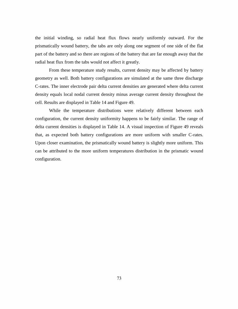
73

the initial winding, so radial heat flux flows nearly uniformly outward. For the

prismatically wound battery, the tabs are only along one segment of one side of the flat

part of the battery and so there are regions of the battery that are far enough away that the

radial heat flux from the tabs would not affect it greatly.

From these temperature study results, current density may be affected by battery

geometry as well. Both battery configurations are simulated at the same three discharge

C-rates. The inner electrode pair delta current densities are generated where delta current

density equals local nodal current density minus average current density throughout the

cell. Results are displayed in Table 14 and Figure 49.

While the temperature distributions were relatively different between each

configuration, the current density uniformity happens to be fairly similar. The range of

delta current densities is displayed in Table 14. A visual inspection of Figure 49 reveals

that, as expected both battery configurations are more uniform with smaller C-rates.

Upon closer examination, the prismatically wound battery is slightly more uniform. This

can be attributed to the more uniform temperatures distribution in the prismatic wound

configuration.

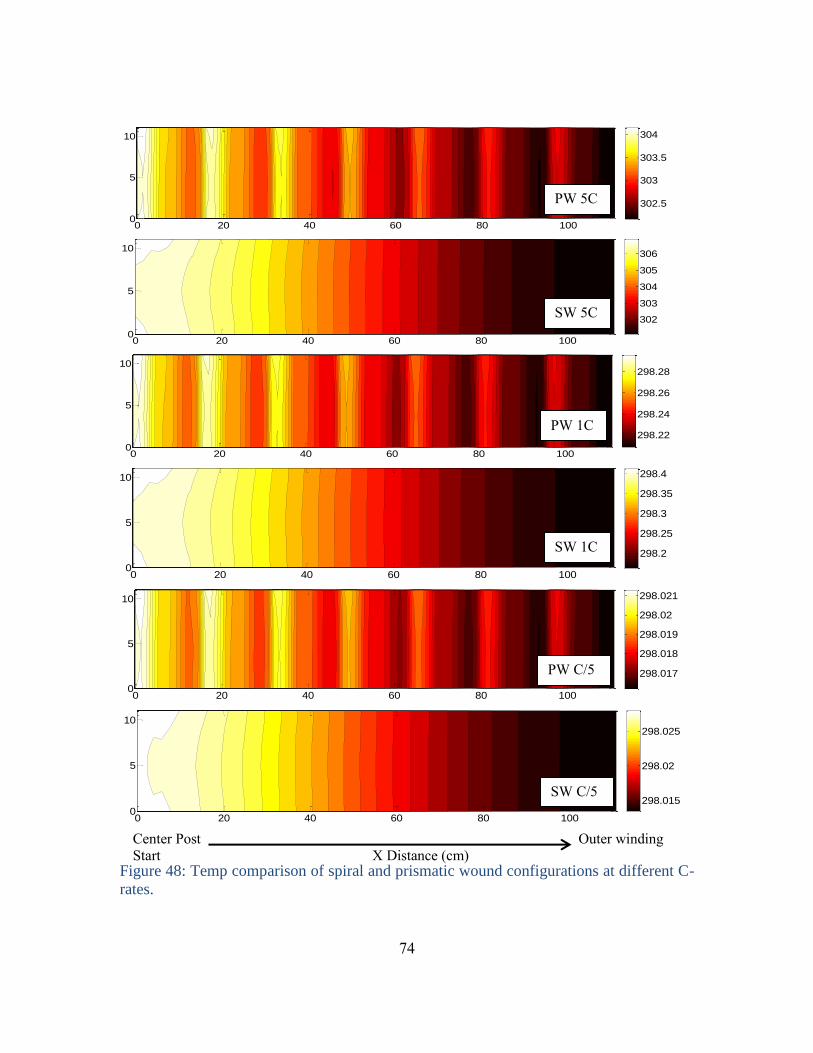
74

Figure 48: Temp comparison of spiral and prismatic wound configurations at different C-

rates.

0 20 40 60 80 1000

5

10

302.5

303

303.5

304

0 20 40 60 80 1000

5

10

302

303

304

305

306

0 20 40 60 80 1000

5

10

298.22

298.24

298.26

298.28

0 20 40 60 80 1000

5

10

298.2

298.25

298.3

298.35

298.4

0 20 40 60 80 1000

5

10

298.017

298.018

298.019

298.02

298.021

0 20 40 60 80 1000

5

10

298.015

298.02

298.025

Center Post Outer winding

Start X Distance (cm)

SW C/5

PW C/5

PW 1C

PW 5C

SW 1C

SW 5C

75

Figure 49: Current density comparison of spiral and prismatic wound configurations at

different C-rates.

0 20 40 60 80 1000

5

10

-5

0

5

10x 10

-3

0 20 40 60 80 1000

5

10

-5

0

5

x 10-3

0 20 40 60 80 1000

5

10

-5

0

5

10x 10

-3

0 20 40 60 80 1000

5

10

-5

0

5

x 10-3

0 20 40 60 80 1000

5

10

-5

0

5

10x 10

-3

0 20 40 60 80 1000

5

10

-5

0

5

x 10-3

SW 5C

SW 1C

SW C/5

PW 5C

PW 1C

PW C/5

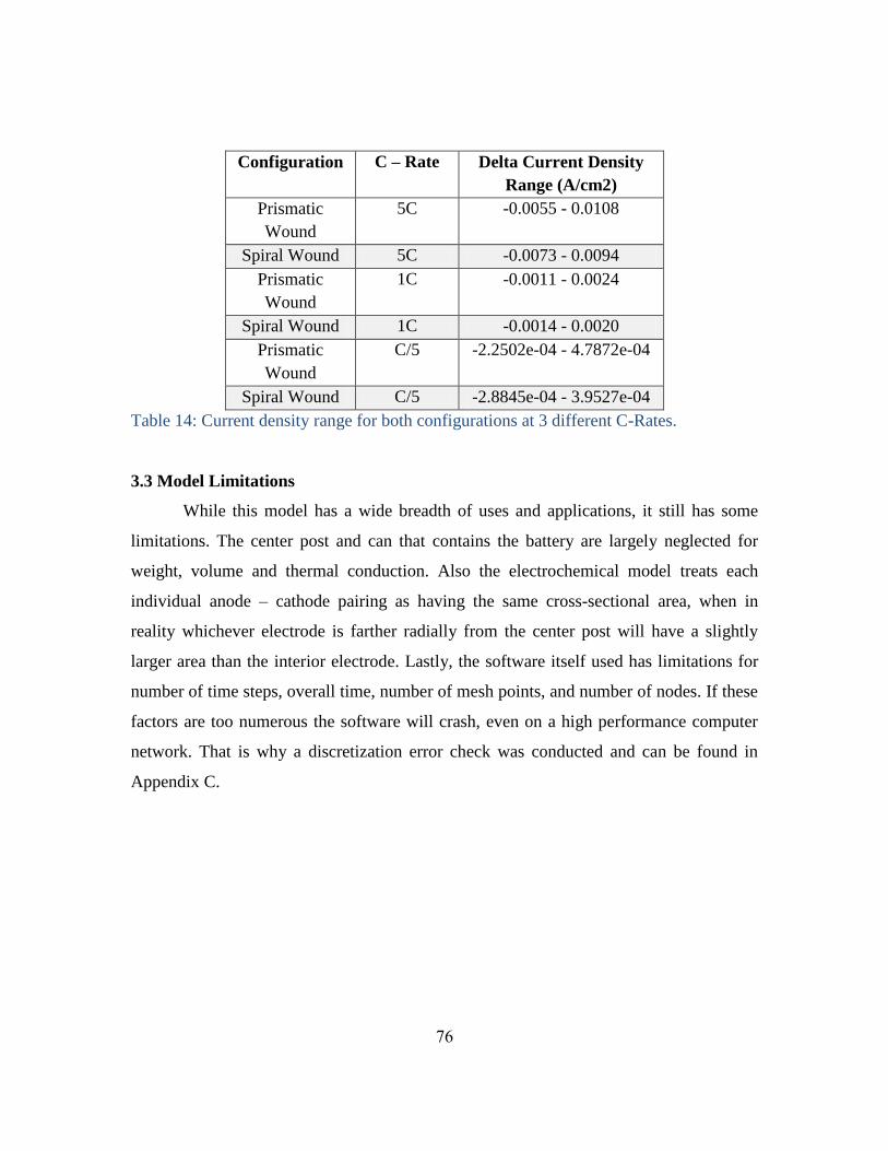
76

Configuration C – Rate

Delta Current Density

Range (A/cm2)

Prismatic

Wound

5C -0.0055 - 0.0108

Spiral Wound 5C -0.0073 - 0.0094

Prismatic

Wound

1C -0.0011 - 0.0024

Spiral Wound 1C -0.0014 - 0.0020

Prismatic

Wound

C/5 -2.2502e-04 - 4.7872e-04

Spiral Wound C/5 -2.8845e-04 - 3.9527e-04

Table 14: Current density range for both configurations at 3 different C-Rates.

3.3 Model Limitations

While this model has a wide breadth of uses and applications, it still has some

limitations. The center post and can that contains the battery are largely neglected for

weight, volume and thermal conduction. Also the electrochemical model treats each

individual anode – cathode pairing as having the same cross-sectional area, when in

reality whichever electrode is farther radially from the center post will have a slightly

larger area than the interior electrode. Lastly, the software itself used has limitations for

number of time steps, overall time, number of mesh points, and number of nodes. If these

factors are too numerous the software will crash, even on a high performance computer

network. That is why a discretization error check was conducted and can be found in

Appendix C.

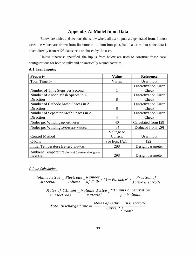
77

Appendix A: Model Input Data

Below are tables and sections that show where all user inputs are generated from. In most

cases the values are drawn from literature on lithium iron phosphate batteries, but some data is

taken directly from A123 datasheets or chosen by the user.

Unless otherwise specified, the inputs from below are used to construct “base case”

configurations for both spirally and prismatically wound batteries.

A.1 User Inputs:

Property Value Reference

Total Time (s) Varies User input

Number of Time Steps per Second 1

Discretization Error

Check

Number of Anode Mesh Spaces in Z

Direction 8

Discretization Error

Check

Number of Cathode Mesh Spaces in Z

Direction 8

Discretization Error

Check

Number of Separator Mesh Spaces in Z

Direction 4

Discretization Error

Check

Nodes per Winding (spirally wound) 40 Calculated from [29]

Nodes per Winding (prismatically wound) 84 Deduced from [29]

Control Method

Voltage or

Current User input

C-Rate See Eqn. [A.1] [22]

Initial Temperature Battery (Kelvin) 298 Design parameter

Ambient Temperature (Kelvin) (constant throughout

simulation) 298 Design parameter

C-Rate Calculation:

( )

⁄

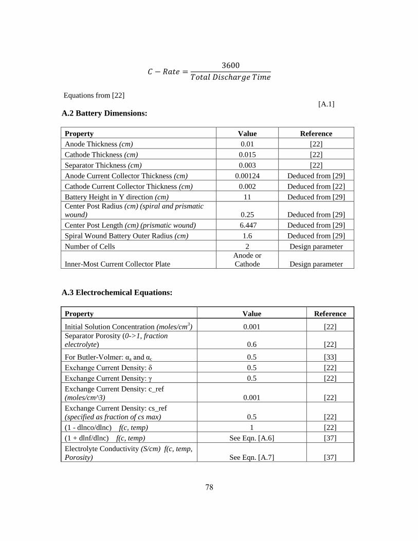
78

Equations from [22]

[A.1]

A.2 Battery Dimensions:

Property Value Reference

Anode Thickness (cm) 0.01 [22]

Cathode Thickness (cm) 0.015 [22]

Separator Thickness (cm) 0.003 [22]

Anode Current Collector Thickness (cm) 0.00124 Deduced from [29]

Cathode Current Collector Thickness (cm) 0.002 Deduced from [22]

Battery Height in Y direction (cm) 11 Deduced from [29]

Center Post Radius (cm) (spiral and prismatic

wound) 0.25 Deduced from [29]

Center Post Length (cm) (prismatic wound) 6.447 Deduced from [29]

Spiral Wound Battery Outer Radius (cm) 1.6 Deduced from [29]

Number of Cells 2 Design parameter

Inner-Most Current Collector Plate

Anode or

Cathode Design parameter

A.3 Electrochemical Equations:

Property Value Reference

Initial Solution Concentration (moles/cm3) 0.001 [22]

Separator Porosity (0->1, fraction

electrolyte) 0.6 [22]

For Butler-Volmer: αa and αc 0.5 [33]

Exchange Current Density: δ 0.5 [22]

Exchange Current Density: γ 0.5 [22]

Exchange Current Density: c_ref

(moles/cm^3) 0.001 [22]

Exchange Current Density: cs_ref

(specified as fraction of cs max) 0.5 [22]

(1 - dlnco/dlnc) f(c, temp) 1 [22]

(1 + dlnf/dlnc) f(c, temp) See Eqn. [A.6] [37]

Electrolyte Conductivity (S/cm) f(c, temp,

Porosity) See Eqn. [A.7] [37]

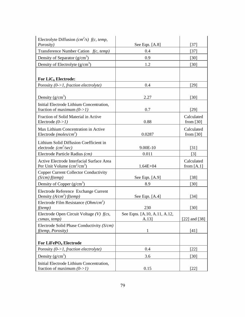
79

Electrolyte Diffusion (cm2/s) f(c, temp,

Porosity) See Eqn. [A.8] [37]

Transference Number Cation f(c, temp) 0.4 [37]

Density of Separator (g/cm3) 0.9 [30]

Density of Electrolyte (g/cm3) 1.2 [30]

For LiC6 Electrode:

Porosity (0->1, fraction electrolyte) 0.4 [29]

Density (g/cm3) 2.27 [30]

Initial Electrode Lithium Concentration,

fraction of maximum (0->1) 0.7 [29]

Fraction of Solid Material in Active

Electrode (0->1) 0.88

Calculated

from [30]

Max Lithium Concentration in Active

Electrode (moles/cm3) 0.0287

Calculated

from [30]

Lithium Solid Diffusion Coefficient in

electrode (cm2/sec) 9.00E-10 [31]

Electrode Particle Radius (cm) 0.011 [3]

Active Electrode Interfacial Surface Area

Per Unit Volume (cm2/cm

3) 1.64E+04

Calculated

from [A.1]

Copper Current Collector Conductivity

(S/cm) f(temp) See Eqn. [A.9] [38]

Density of Copper (g/cm3) 8.9 [30]

Electrode Reference Exchange Current

Density (A/cm2) f(temp) See Eqn. [A.4] [34]

Electrode Film Resistance (Ohm/cm2)

f(temp) 230 [30]

Electrode Open Circuit Voltage (V) f(cs,

csmax, temp)

See Eqns. [A.10, A.11, A.12,

A.13] [22] and [38]

Electrode Solid Phase Conductivity (S/cm)

f(temp, Porosity) 1 [41]

For LiFePO4 Electrode

Porosity (0->1, fraction electrolyte) 0.4 [22]

Density (g/cm3) 3.6 [30]

Initial Electrode Lithium Concentration,

fraction of maximum (0->1) 0.15 [22]

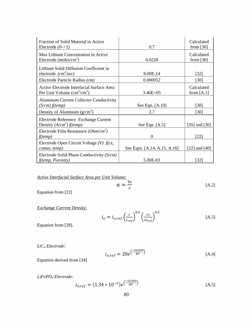
80

Fraction of Solid Material in Active

Electrode (0->1) 0.7

Calculated

from [30]

Max Lithium Concentration in Active

Electrode (moles/cm3) 0.0228

Calculated

from [30]

Lithium Solid Diffusion Coefficient in

electrode (cm2/sec) 8.00E-14 [32]

Electrode Particle Radius (cm) 0.000052 [30]

Active Electrode Interfacial Surface Area

Per Unit Volume (cm2/cm

3) 3.46E+05

Calculated

from [A.1]

Aluminum Current Collector Conductivity

(S/cm) f(temp) See Eqn. [A.10] [38]

Density of Aluminum (g/cm3) 2.7 [30]

Electrode Reference Exchange Current

Density (A/cm2) f(temp) See Eqn. [A.5] [35] and [36]

Electrode Film Resistance (Ohm/cm2)

f(temp) 0 [22]

Electrode Open Circuit Voltage (V) f(cs,

csmax, temp) See Eqns. [A.14, A.15, A.16] [22] and [40]

Electrode Solid Phase Conductivity (S/cm)

f(temp, Porosity) 5.00E-03 [32]

Active Interfacial Surface Area per Unit Volume:

[A.2]

Equation from [22]

Exchange Current Density:

(

)

(

)

[A.3]

Equation from [28].

LiC6 Electrode:

(

) [A.4]

Equation derived from [34]

LiFePO4 Electrode:

( ) (

) [A.5]

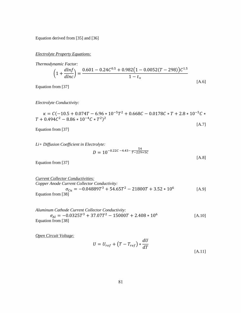
81

Equation derived from [35] and [36]

Electrolyte Property Equations:

Thermodynamic Factor:

(

)

( ( ))

[A.6]

Equation from [37]

Electrolyte Conductivity:

( )

[A.7]

Equation from [37]

Li+ Diffusion Coefficient in Electrolyte:

[A.8]

Equation from [37]

Current Collector Conductivities:

Copper Anode Current Collector Conductivity:

[A.9]

Equation from [38]

Aluminum Cathode Current Collector Conductivity:

[A.10]

Equation from [38]

Open Circuit Voltage:

( )

[A.11]

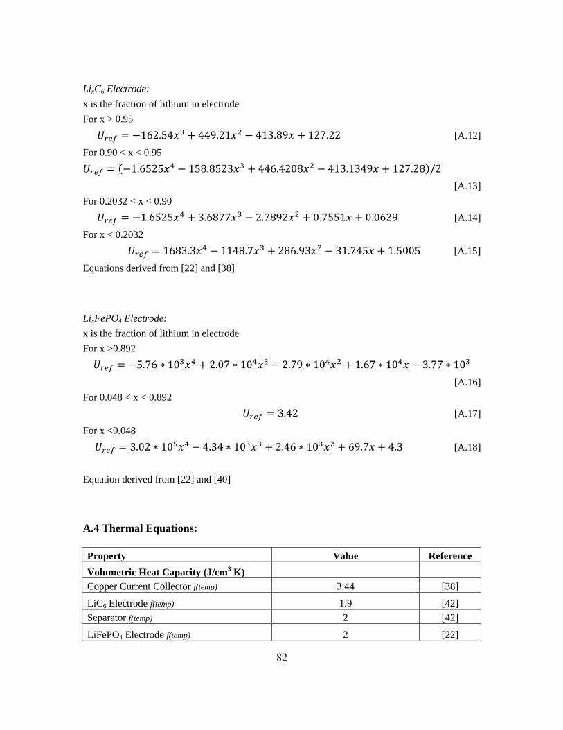
82

LixC6 Electrode:

x is the fraction of lithium in electrode

For x > 0.95

[A.12]

For 0.90 < x < 0.95

( )

[A.13]

For 0.2032 < x < 0.90

[A.14]

For x < 0.2032

[A.15]

Equations derived from [22] and [38]

LixFePO4 Electrode:

x is the fraction of lithium in electrode

For x >0.892

[A.16]

For 0.048 < x < 0.892

[A.17]

For x <0.048

[A.18]

Equation derived from [22] and [40]

A.4 Thermal Equations:

Property Value Reference

Volumetric Heat Capacity (J/cm3 K)

Copper Current Collector f(temp) 3.44 [38]

LiC6 Electrode f(temp) 1.9 [42]

Separator f(temp) 2 [42]

LiFePO4 Electrode f(temp) 2 [22]

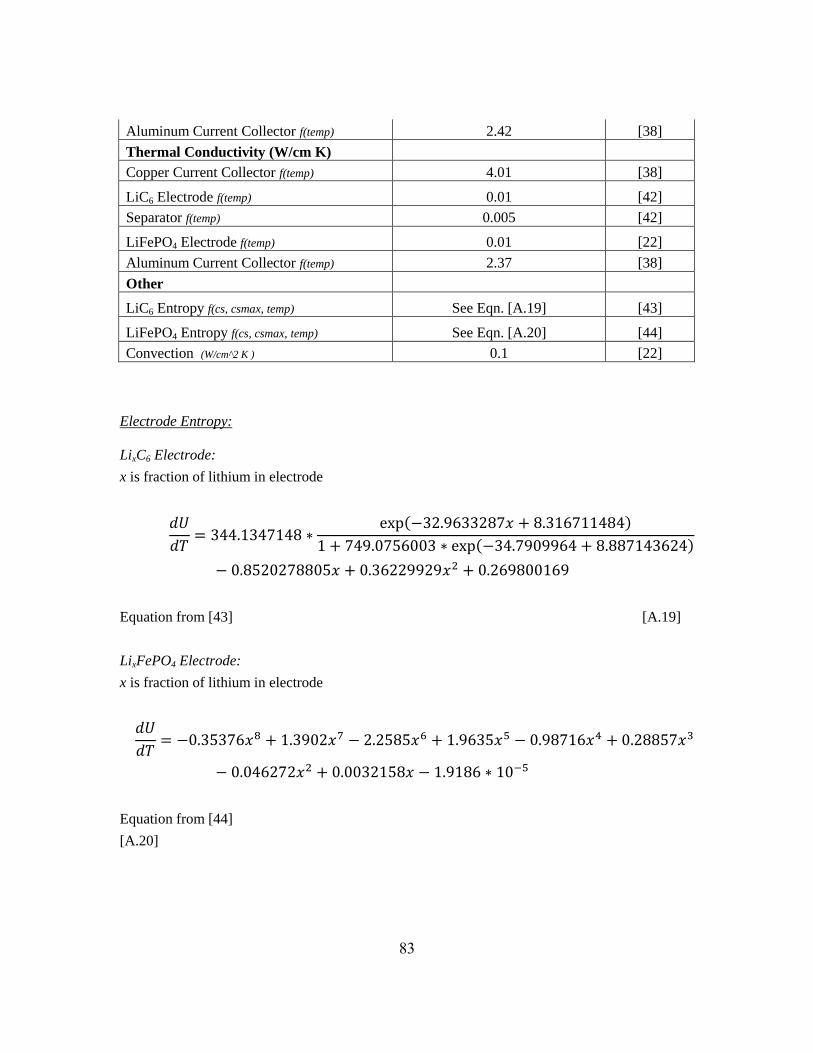
83

Aluminum Current Collector f(temp) 2.42 [38]

Thermal Conductivity (W/cm K)

Copper Current Collector f(temp) 4.01 [38]

LiC6 Electrode f(temp) 0.01 [42]

Separator f(temp) 0.005 [42]

LiFePO4 Electrode f(temp) 0.01 [22]

Aluminum Current Collector f(temp) 2.37 [38]

Other

LiC6 Entropy f(cs, csmax, temp) See Eqn. [A.19] [43]

LiFePO4 Entropy f(cs, csmax, temp) See Eqn. [A.20] [44]

Convection (W/cm^2 K ) 0.1 [22]

Electrode Entropy:

LixC6 Electrode:

x is fraction of lithium in electrode

( )

( )

Equation from [43] [A.19]

LixFePO4 Electrode:

x is fraction of lithium in electrode

Equation from [44]

[A.20]

84

A.5 List of Symbols:

Symbol

Meaning

a Active Interfacial Surface Area per Unit Volume

ɛ Porosity

αa Anodic charge transfer coefficient

αc Cathodic charge transfer coefficient

R Gas Constant, 8.314

T Temperature (Kelvin unless noted otherwise)

C Lithium ion concentration in Molarity

t+ Li+ transference number

io Exchange current density

σ Conductivity

U Open circuit potential

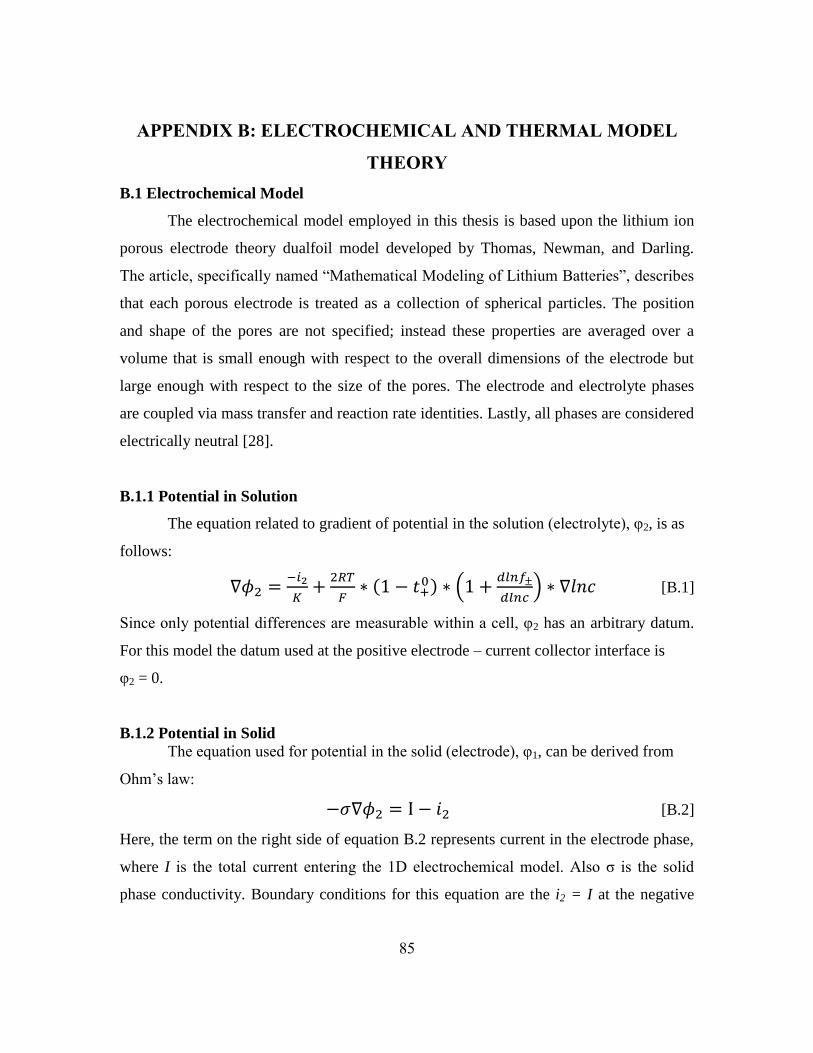
85

APPENDIX B: ELECTROCHEMICAL AND THERMAL MODEL

THEORY

B.1 Electrochemical Model

The electrochemical model employed in this thesis is based upon the lithium ion

porous electrode theory dualfoil model developed by Thomas, Newman, and Darling.

The article, specifically named “Mathematical Modeling of Lithium Batteries”, describes

that each porous electrode is treated as a collection of spherical particles. The position

and shape of the pores are not specified; instead these properties are averaged over a

volume that is small enough with respect to the overall dimensions of the electrode but

large enough with respect to the size of the pores. The electrode and electrolyte phases

are coupled via mass transfer and reaction rate identities. Lastly, all phases are considered

electrically neutral [28].

B.1.1 Potential in Solution

The equation related to gradient of potential in the solution (electrolyte), φ2, is as

follows:

(

) (

) [B.1]

Since only potential differences are measurable within a cell, φ2 has an arbitrary datum.

For this model the datum used at the positive electrode – current collector interface is

φ2 = 0.

B.1.2 Potential in Solid

The equation used for potential in the solid (electrode), φ1, can be derived from

Ohm’s law:

[B.2]

Here, the term on the right side of equation B.2 represents current in the electrode phase,

where I is the total current entering the 1D electrochemical model. Also σ is the solid

phase conductivity. Boundary conditions for this equation are the i2 = I at the negative

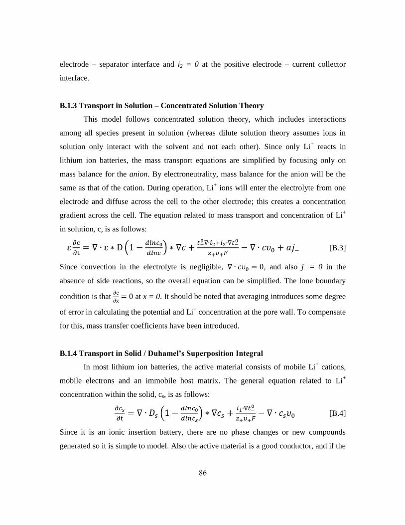
86

electrode – separator interface and i2 = 0 at the positive electrode – current collector

interface.

B.1.3 Transport in Solution – Concentrated Solution Theory

This model follows concentrated solution theory, which includes interactions

among all species present in solution (whereas dilute solution theory assumes ions in

solution only interact with the solvent and not each other). Since only Li+ reacts in

lithium ion batteries, the mass transport equations are simplified by focusing only on

mass balance for the anion. By electroneutrality, mass balance for the anion will be the

same as that of the cation. During operation, Li+ ions will enter the electrolyte from one

electrode and diffuse across the cell to the other electrode; this creates a concentration

gradient across the cell. The equation related to mass transport and concentration of Li+

in solution, c, is as follows:

(

)

[B.3]

Since convection in the electrolyte is negligible, , and also j- = 0 in the

absence of side reactions, so the overall equation can be simplified. The lone boundary

condition is that

at x = 0. It should be noted that averaging introduces some degree

of error in calculating the potential and Li+ concentration at the pore wall. To compensate

for this, mass transfer coefficients have been introduced.

B.1.4 Transport in Solid / Duhamel’s Superposition Integral

In most lithium ion batteries, the active material consists of mobile Li+ cations,

mobile electrons and an immobile host matrix. The general equation related to Li+

concentration within the solid, cs, is as follows:

(

)

[B.4]

Since it is an ionic insertion battery, there are no phase changes or new compounds

generated so it is simple to model. Also the active material is a good conductor, and if the

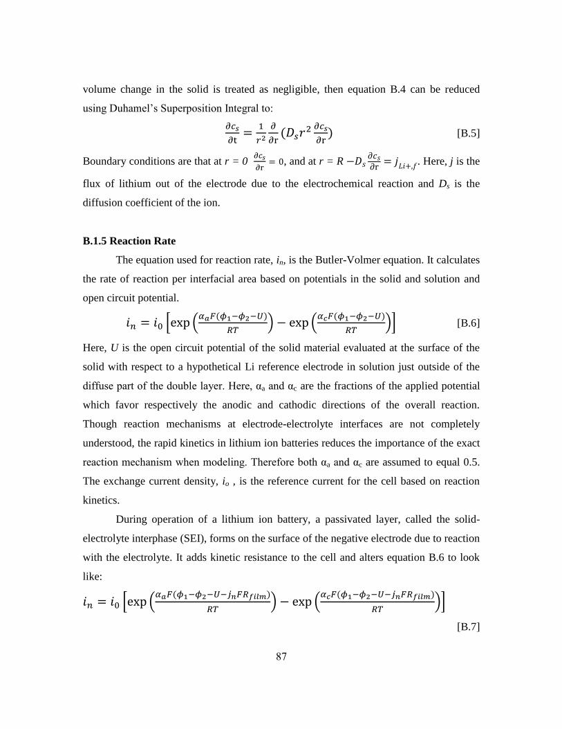
87

volume change in the solid is treated as negligible, then equation B.4 can be reduced

using Duhamel’s Superposition Integral to:

(

) [B.5]

Boundary conditions are that at r = 0

, and at r = R

. Here, j is the

flux of lithium out of the electrode due to the electrochemical reaction and Ds is the

diffusion coefficient of the ion.

B.1.5 Reaction Rate

The equation used for reaction rate, in, is the Butler-Volmer equation. It calculates

the rate of reaction per interfacial area based on potentials in the solid and solution and

open circuit potential.

[ ( ( )

) (

( )

)] [B.6]

Here, U is the open circuit potential of the solid material evaluated at the surface of the

solid with respect to a hypothetical Li reference electrode in solution just outside of the

diffuse part of the double layer. Here, αa and αc are the fractions of the applied potential

which favor respectively the anodic and cathodic directions of the overall reaction.

Though reaction mechanisms at electrode-electrolyte interfaces are not completely

understood, the rapid kinetics in lithium ion batteries reduces the importance of the exact

reaction mechanism when modeling. Therefore both αa and αc are assumed to equal 0.5.

The exchange current density, io , is the reference current for the cell based on reaction

kinetics.

During operation of a lithium ion battery, a passivated layer, called the solid-

electrolyte interphase (SEI), forms on the surface of the negative electrode due to reaction

with the electrolyte. It adds kinetic resistance to the cell and alters equation B.6 to look

like:

[ ( ( )

) (

( )

)]

[B.7]

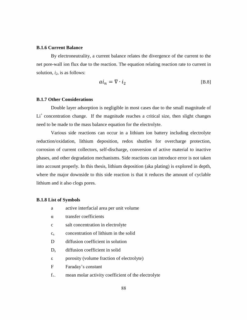
88

B.1.6 Current Balance

By electroneutrality, a current balance relates the divergence of the current to the

net pore-wall ion flux due to the reaction. The equation relating reaction rate to current in

solution, i2, is as follows:

[B.8]

B.1.7 Other Considerations

Double layer adsorption is negligible in most cases due to the small magnitude of

Li+

concentration change. If the magnitude reaches a critical size, then slight changes

need to be made to the mass balance equation for the electrolyte.

Various side reactions can occur in a lithium ion battery including electrolyte

reduction/oxidation, lithium deposition, redox shuttles for overcharge protection,

corrosion of current collectors, self-discharge, conversion of active material to inactive

phases, and other degradation mechanisms. Side reactions can introduce error is not taken

into account properly. In this thesis, lithium deposition (aka plating) is explored in depth,

where the major downside to this side reaction is that it reduces the amount of cyclable

lithium and it also clogs pores.

B.1.8 List of Symbols

a active interfacial area per unit volume

α transfer coefficients

c salt concentration in electrolyte

cs concentration of lithium in the solid

D diffusion coefficient in solution

Ds diffusion coefficient in solid

ε porosity (volume fraction of electrolyte)

F Faraday’s constant

f+- mean molar activity coefficient of the electrolyte

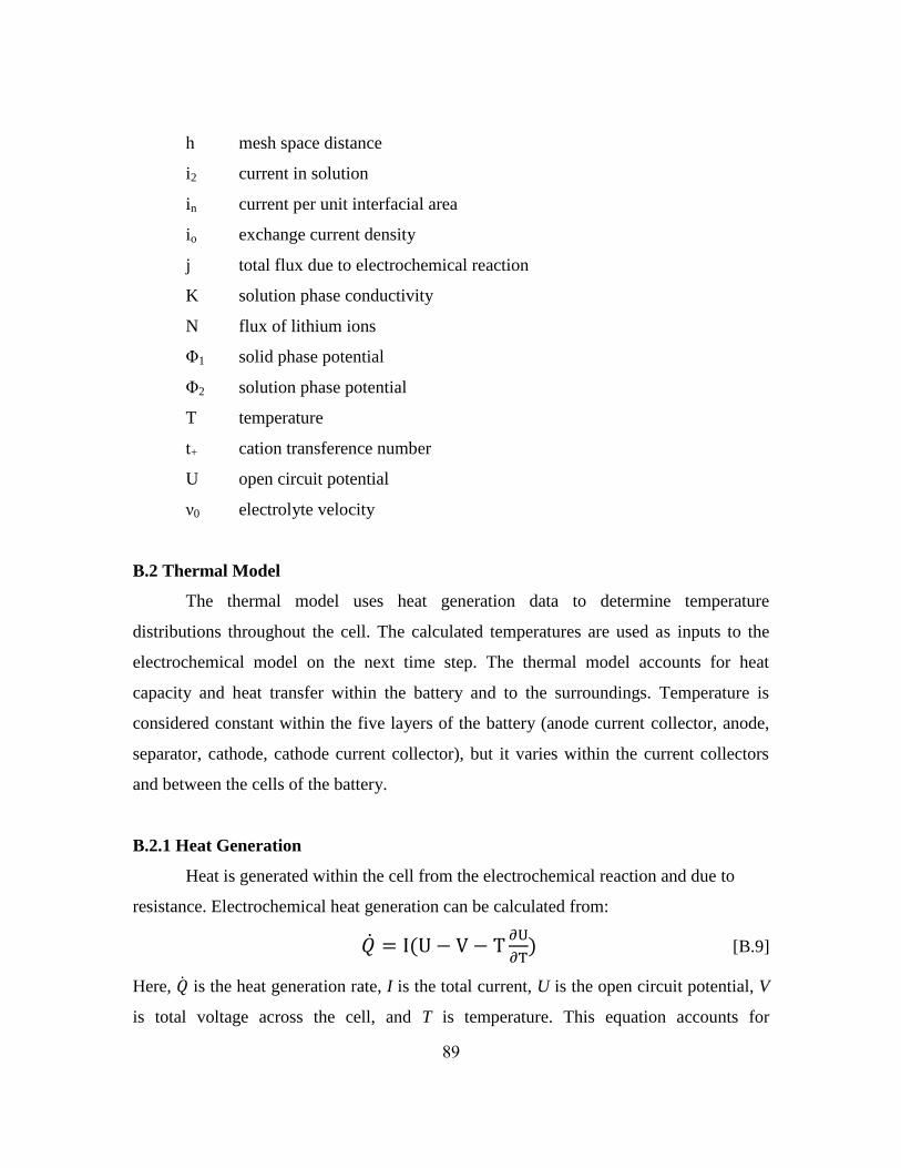
89

h mesh space distance

i2 current in solution

in current per unit interfacial area

io exchange current density

j total flux due to electrochemical reaction

K solution phase conductivity

N flux of lithium ions

Φ1 solid phase potential

Φ2 solution phase potential

T temperature

t+ cation transference number

U open circuit potential

ν0 electrolyte velocity

B.2 Thermal Model

The thermal model uses heat generation data to determine temperature

distributions throughout the cell. The calculated temperatures are used as inputs to the

electrochemical model on the next time step. The thermal model accounts for heat

capacity and heat transfer within the battery and to the surroundings. Temperature is

considered constant within the five layers of the battery (anode current collector, anode,

separator, cathode, cathode current collector), but it varies within the current collectors

and between the cells of the battery.

B.2.1 Heat Generation

Heat is generated within the cell from the electrochemical reaction and due to

resistance. Electrochemical heat generation can be calculated from:

(

) [B.9]

Here, is the heat generation rate, I is the total current, U is the open circuit potential, V

is total voltage across the cell, and T is temperature. This equation accounts for

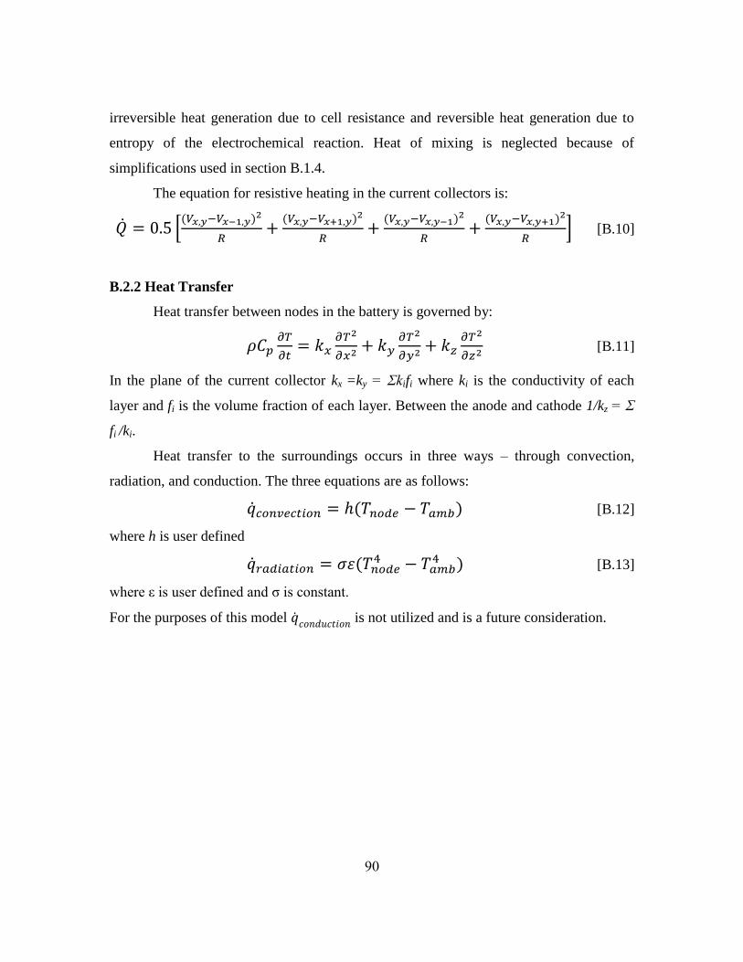
90

irreversible heat generation due to cell resistance and reversible heat generation due to

entropy of the electrochemical reaction. Heat of mixing is neglected because of

simplifications used in section B.1.4.

The equation for resistive heating in the current collectors is:

[( )

( )

( )

( )

] [B.10]

B.2.2 Heat Transfer

Heat transfer between nodes in the battery is governed by:

[B.11]

In the plane of the current collector kx =ky = Σkifi where ki is the conductivity of each

layer and fi is the volume fraction of each layer. Between the anode and cathode 1/kz = Σ

fi /ki.

Heat transfer to the surroundings occurs in three ways – through convection,

radiation, and conduction. The three equations are as follows:

( ) [B.12]

where h is user defined

(

) [B.13]

where ε is user defined and σ is constant.

For the purposes of this model is not utilized and is a future consideration.

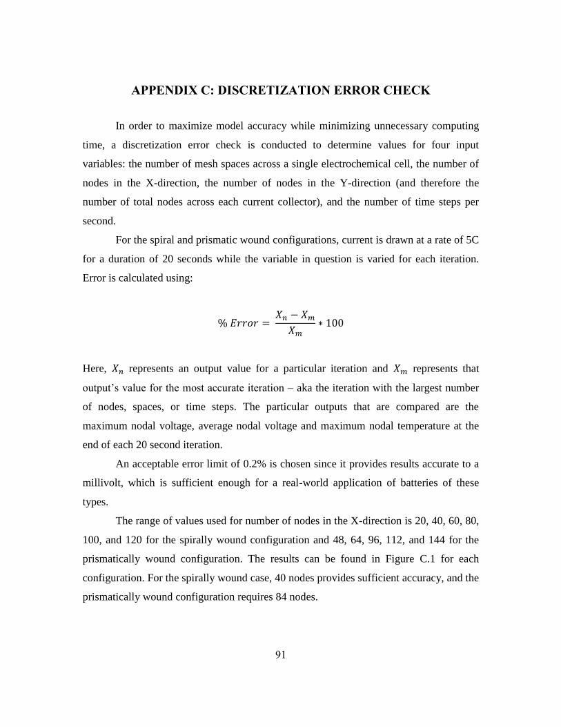
91

APPENDIX C: DISCRETIZATION ERROR CHECK

In order to maximize model accuracy while minimizing unnecessary computing

time, a discretization error check is conducted to determine values for four input

variables: the number of mesh spaces across a single electrochemical cell, the number of

nodes in the X-direction, the number of nodes in the Y-direction (and therefore the

number of total nodes across each current collector), and the number of time steps per

second.

For the spiral and prismatic wound configurations, current is drawn at a rate of 5C

for a duration of 20 seconds while the variable in question is varied for each iteration.

Error is calculated using:

Here, represents an output value for a particular iteration and represents that

output’s value for the most accurate iteration – aka the iteration with the largest number

of nodes, spaces, or time steps. The particular outputs that are compared are the

maximum nodal voltage, average nodal voltage and maximum nodal temperature at the

end of each 20 second iteration.

An acceptable error limit of 0.2% is chosen since it provides results accurate to a

millivolt, which is sufficient enough for a real-world application of batteries of these

types.

The range of values used for number of nodes in the X-direction is 20, 40, 60, 80,

100, and 120 for the spirally wound configuration and 48, 64, 96, 112, and 144 for the

prismatically wound configuration. The results can be found in Figure C.1 for each

configuration. For the spirally wound case, 40 nodes provides sufficient accuracy, and the

prismatically wound configuration requires 84 nodes.

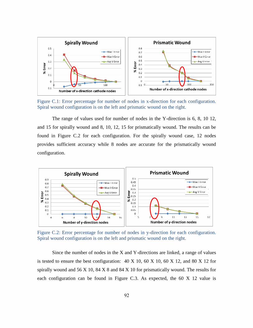
92

Figure C.1: Error percentage for number of nodes in x-direction for each configuration.

Spiral wound configuration is on the left and prismatic wound on the right.

The range of values used for number of nodes in the Y-direction is 6, 8, 10 12,

and 15 for spirally wound and 8, 10, 12, 15 for prismatically wound. The results can be

found in Figure C.2 for each configuration. For the spirally wound case, 12 nodes

provides sufficient accuracy while 8 nodes are accurate for the prismatically wound

configuration.

Figure C.2: Error percentage for number of nodes in y-direction for each configuration.

Spiral wound configuration is on the left and prismatic wound on the right.

Since the number of nodes in the X and Y-directions are linked, a range of values

is tested to ensure the best configuration: 40 X 10, 60 X 10, 60 X 12, and 80 X 12 for

spirally wound and 56 X 10, 84 X 8 and 84 X 10 for prismatically wound. The results for

each configuration can be found in Figure C.3. As expected, the 60 X 12 value is

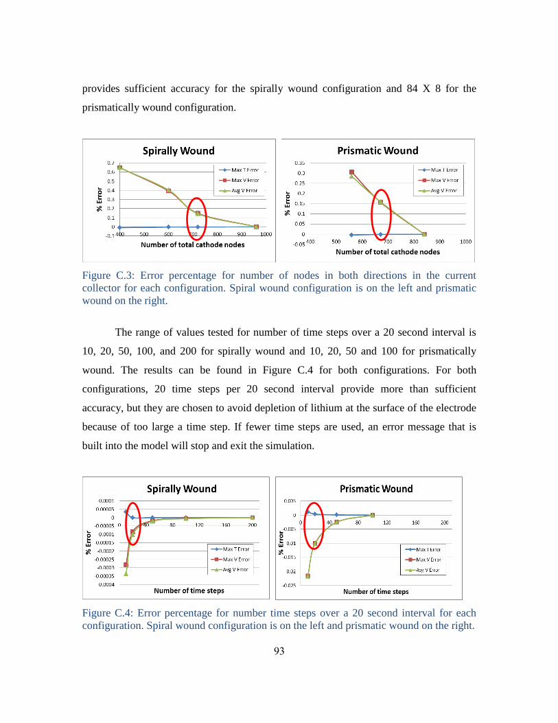
93

provides sufficient accuracy for the spirally wound configuration and 84 X 8 for the

prismatically wound configuration.

Figure C.3: Error percentage for number of nodes in both directions in the current

collector for each configuration. Spiral wound configuration is on the left and prismatic

wound on the right.

The range of values tested for number of time steps over a 20 second interval is

10, 20, 50, 100, and 200 for spirally wound and 10, 20, 50 and 100 for prismatically

wound. The results can be found in Figure C.4 for both configurations. For both

configurations, 20 time steps per 20 second interval provide more than sufficient

accuracy, but they are chosen to avoid depletion of lithium at the surface of the electrode

because of too large a time step. If fewer time steps are used, an error message that is

built into the model will stop and exit the simulation.

Figure C.4: Error percentage for number time steps over a 20 second interval for each

configuration. Spiral wound configuration is on the left and prismatic wound on the right.

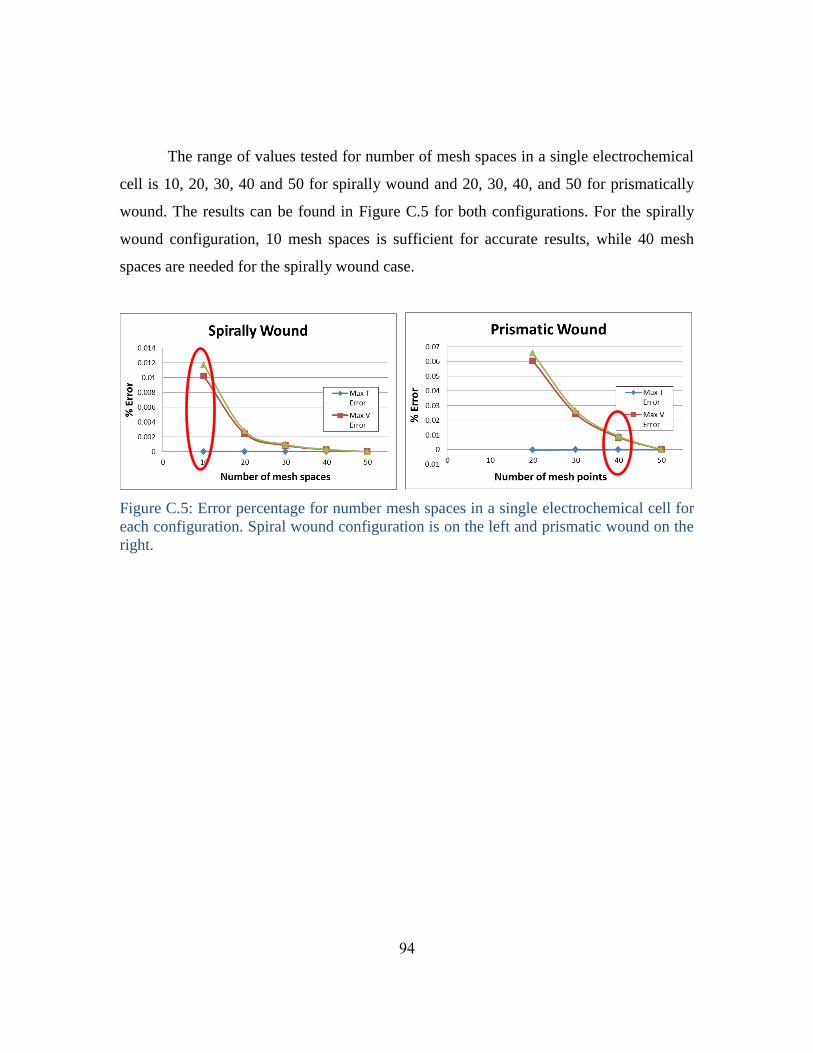
94

The range of values tested for number of mesh spaces in a single electrochemical

cell is 10, 20, 30, 40 and 50 for spirally wound and 20, 30, 40, and 50 for prismatically

wound. The results can be found in Figure C.5 for both configurations. For the spirally

wound configuration, 10 mesh spaces is sufficient for accurate results, while 40 mesh

spaces are needed for the spirally wound case.

Figure C.5: Error percentage for number mesh spaces in a single electrochemical cell for

each configuration. Spiral wound configuration is on the left and prismatic wound on the

right.

95

References

[1] X. Zhang, “Thermal Analysis of a Cylindrical Lithium-ion Battery,” Electrochemica

Acta, vol. 56, 2011, pp. 1246-1255.

[2] M. Doyle, T.F. Fuller, J. Newman, “Modeling of Galvanostatic Charge and Discharge

of the Lithium/Polymer/Insertion Cell,” Journal of The Electrochemical Society, vol.

140, 1993, pp. 1526-1533.

[3] T.F. Fuller, M. Doyle, J. Newman, “Simulation and Optimization of Dual Lithium Ion

Insertion Cell,” Journal of The Electrochemical Society, vol. 141, 1994, pp. 1-10.

[4] M. Doyle, J. Newman, “Comparison of Modeling Predictions with Experimental Data

from Plastic Lithium Ion Cells,” Journal of The Electrochemical Society, vol. 143,

1996, pp. 1890-1903.

[5] D.M. Bernardi, H. Gu, and A.Y. Schoene, “Two-Dimensional Mathematical Model of

a Lead-Acid Cell,” Journal of The Electrochemical Society, vol. 140, 1993, pp.

2250-2258.

[6] T.I. Evans and R.E. White, “A Thermal Analysis of a Spirally Wound Battery Using a

Simple Mathematical Model,” Journal of The Electrochemical Society, vol. 136,

1989, pp. 2145-2152.

[7] J. Lee, K.W. Choi, N.P. Yao, and C.C. Christianson, “Three-Dimensional Thermal

Modeling of Electric Vehicle Batteries,” Journal of The Electrochemical Society,

vol. 133, Jul. 1986, pp. 1286-1291.

[8] M.W. Verbrugge, “Three-dimensional temperature and current distribution in a

battery module,” AIChE Journal, vol. 41, 1995, pp. 1550-1562.

[9] D.R. Baker and M.W. Verbrugge, “Temperature and Current Distribution in Thin-

Film Batteries,” Journal of The Electrochemical Society, vol. 146, Jul. 1999, pp.

2413-2424.

[10] D. Bharathan, A. Pesaran, A. Vlahinos, and G. Kim, “Improving battery design with

electro-thermal modeling,” Vehicle Power and Propulsion, 2005 IEEE Conference,

2005, p. 8 pp.

[11] Y. Inui, Y. Kobayashi, Y. Watanabe, Y. Watase, and Y. Kitamura, “Simulation of

temperature distribution in cylindrical and prismatic lithium ion secondary

batteries,” Energy Conversion and Management, vol. 48, Jul. 2007, pp. 2103-2109.

[12] J.N. Reimers, “Predicting current flow in spiral wound cell geometries,” Journal of

Power Sources, vol. 158, Jul. 2006, pp. 663-672.

[13] J.N. Harb and R.M. LaFollette, “Mathematical Model of the Discharge Behavior of a

Spirally Wound Lead-Acid Cell,” Journal of The Electrochemical Society, vol. 146,

Mar. 1999, pp. 809-818.

[14] Harb, John N, “The Influence of Current Distribution on Battery Design and

Performance,” May. 2009.

[15] Gi-Heon Kim, Smith, Kandler, and Ahmad, Pesaran, “Three-Dimensional

Electrochemical Thermal Coupled Model of Large Format Cylindrical Lithium Ion

Cells,” Oct. 2007.

96

[16] D.H. Jeon, S.M. Baek, “Thermal Modeling of Cylindrical Lithium Ion Battery

During Discharge Cycle,” Energy Conservation and Management, vol. 52, August

2011, pp. 2973-2981.

[17] X. Zhang, “Thermal Analysis of a Cylindrical Lithium-ion Battery,” Electrochemica

Acta, vol. 56, Jan. 2011, pp. 1246-1255.

[18] Y.S. Chen, C.C.Hu, Y.Y. Li, “The Importance of Heat Evolution During the

Overcharge Process and the Protection Mechanism of Electrolyte Additives for

Prismatic Lithium Ion Batteries,” Journal of Power Sources, vol. 181, June 2008, pp.

69-73.

[19] J.F. Cousseau, C. Siret, P. Biensan, M. Broussely, “Recent Developments in Li-ion

Prismatic Cells,” Journal of Power Sources, vol. 162, Nov. 2006, pp. 790-796.

[20] K. Kumaresan, G. Sikha, and R.E. White, “Thermal Model for a Li-Ion Cell,”

Journal of The Electrochemical Society, vol. 155, Feb. 2008, pp. A164-A171.

[21] C.R. Pals and J. Newman, “Thermal Modeling of the Lithium/Polymer Battery,”

Journal of The Electrochemical Society, vol. 142, Oct. 1995, pp. 3274-3281.

[22] R. Gerver and J. Meyers, “Three-Dimensional Modeling of Electrochemical

Performance and Heat Generation of Lithium-Ion Batteries in Tabbed Planar

Configurations,” Master’s Thesis, The University of Texas at Austin, 2009.

[23] H.S. Hsu, L.T. Yang, J. Ma, C. Zhu, Ubiquitous Intelligence and Computing,

Springer, 2011.

[24] Weisstein, Eric W. "Archimedes' Spiral." From MathWorld--A Wolfram Web

Resource. http://mathworld.wolfram.com/ArchimedesSpiral.html

[25] T.L. Heath, The Works of Archimedes, Dover Publications, 1897.

[26] J. S. Newman and K.E. Thomas-Alyea, Electrochemical Systems, Wiley-IEEE,

2004.

[27] C.M. Doyle, Design and simulation of lithium rechargeable batteries, 1995.

[28] K. Thomas, J. Newman, and R. Darling, “Mathematical Modeling of Lithium

Batteries,” Advances in Lithium-Ion Batteries, 2002, pp. 345-392.

[29] Nanophosphate High Power Lithium Ion Cell, 2011, A123 Systems, 15 June 2011.

[30] V. Srinivasan and J. Newman, “Design and Optimization of a Natural Graphite/Iron

Phosphate Lithium-Ion Cell,” Journal of The Electrochemical Society, vol. 151, Oct.

2004, pp. A1530-A1538.

[31] S.G. Stewart, V. Srinivasan, and J. Newman, “Modeling the Performance of

Lithium-Ion Batteries and Capacitors during Hybrid-Electric-Vehicle Operation,”

Journal of The Electrochemical Society, vol. 155, 2008, pp. A664-A671.

[32] V. Srinivasan and J. Newman, “Discharge Model for the Lithium Iron-Phosphate

Electrode,” Journal of The Electrochemical Society, vol. 151, Oct. 2004, pp. A1517-

A1529.

[33] J.S. Newman and K.E. Thomas-Alyea, Electrochemical systems, Wiley-IEEE, 2004.

[34] S. Surampudi, E.S. Meeting, E.S.B. Division, and E.S.E.T. Division, Lithium

Batteries, The Electrochemical Society, 2000.

[35] U.S. Kasavajjula, C. Wang, and P.E. Arce, “Discharge Model for LiFePO[sub 4]

Accounting for the Solid Solution Range,” Journal of The Electrochemical Society,

vol. 155, Nov. 2008, pp. A866-A874.

97

[36] M. Takahashi, S. Tobishima, K. Takei, and Y. Sakurai, “Reaction behavior of

LiFePO4 as a cathode material for rechargeable lithium batteries,” Solid State Ionics,

vol. 148, Jun. 2002, pp. 283-289.

[37] L.O. Valoen and J.N. Reimers, “Transport Properties of LiPF[sub 6]-Based Li-Ion

Battery Electrolytes,” Journal of The Electrochemical Society, vol. 152, May. 2005,

pp. A882-A891.

[38] CRC Handbook of Chemistry and Physics, Cleveland, Ohio: CRC Press, 1977.

[39] M.W. Verbrugge and B.J. Koch, “Electrochemical Analysis of Lithiated Graphite

Anodes,” Journal of The Electrochemical Society, vol. 150, Mar. 2003, pp. A374-

A384.

[40] A. Yamada, H. Koizumi, S. Nishimura, N. Sonoyama, R. Kanno, M. Yonemura, T.

Nakamura, and Y. Kobayashi, “Room-temperature miscibility gap in LixFePO4,”

Nat Mater, vol. 5, May. 2006, pp. 357-360.

[41] M. Doyle and Y. Fuentes, “Computer Simulations of a Lithium-Ion Polymer Battery

and Implications for Higher Capacity Next-Generation Battery Designs,” Journal of

The Electrochemical Society, vol. 150, Jun. 2003, pp. A706-A713.

[42] S. Chen, C. Wan, and Y. Wang, “Thermal analysis of lithium-ion batteries,” Journal

of Power Sources, vol. 140, Jan. 2005, pp. 111-124.

[43] V. Srinivasan and C.Y. Wang, “Analysis of Electrochemical and Thermal Behavior

of Li-Ion Cells,” Journal of The Electrochemical Society, vol. 150, Jan. 2003, pp.

A98-A106.

[44] J.L. Dodd, “Phase composition and dynamical studies of lithium iron phosphate,”

May. 2007.

[45] K.J. Lee, G.H. Kim, K. Smith, “3D Thermal and Electrochemical Model for Spirally

Wound Large Format Lithium-ion Batteries,” Oct. 2010.

98

Vita

David Andrew Holmes McCleary was born in Hartford, CT. He spent his first 18

years living in Ellington, CT before going to college at Tufts University in Medford, MA.

There, he earned a Bachelor of Science in Mechanical Engineering in May 2007. At Tufts

he produced an undergraduate thesis on micro thermophotovoltaic cells. After college he

worked for two and a half years at Nuvera Fuel Cells, a PEM fuel cell company in

Billerica, MA. It was there that he developed his passion for electrochemistry while he

prototyped a newly designed fuel cell. At the University of Texas at Austin he worked in

the Meyers Research Group conducting computational modeling on lithium ion batteries.

After graduation David will return to Nuvera Fuel cells where he will work with the fuel

cell that was a prototype when he left and is now the only fuel cell technology used by

the company.

Permanent address: 4 Field Drive

Ellington, CT 06029

This thesis was typed by the author.