copyright by chioke bem harris 2010
TRANSCRIPT

Copyright
by
Chioke Bem Harris
2010

The Thesis committee for Chioke Bem Harriscertifies that this is the approved version of the following thesis:
A Mixed-Integer Model for Optimal Grid-Scale Energy
Storage Allocation
APPROVED BY
SUPERVISING COMMITTEE:
Michael E. Webber, Supervisor
Jeremy P. Meyers, Supervisor

A Mixed-Integer Model for Optimal Grid-Scale Energy
Storage Allocation
by
Chioke Bem Harris, B.S.
THESIS
Presented to the Faculty of the Graduate School of
The University of Texas at Austin
in Partial Fulfillment
of the Requirements
for the Degree of
MASTER OF SCIENCE IN ENGINEERING
The University of Texas at Austin
August 2010

To my girlfriend and parents for their indefatigable support throughout my
development as a scholar.

Acknowledgments
Many thanks to my advisors Dr. Michael Webber and Dr. Jeremy Meyers for
their unending support throughout the development of this work. Additionally, John
Baker, Pat Sweeney, Mark Kapner, Babu Chakka and Eddy Tan from Austin Energy
were all instrumental in providing guidance and the data necessary to make this work
possible.
v
A Mixed-Integer Model for Optimal Grid-Scale Energy
Storage Allocation
Chioke Bem Harris, M.S.E.
The University of Texas at Austin, 2010
Supervisors: Michael E. WebberJeremy P. Meyers
To meet ambitious upcoming state renewable portfolio standards (RPSs), re-
spond to customer demand for “green” electricity choices and to move towards more
renewable, domestic and clean sources of energy, many utilities and power producers
are accelerating deployment of wind, solar photovoltaic and solar thermal generating
facilities. These sources of electricity, particularly wind power, are highly variable
and difficult to forecast. To manage this variability, utilities can increase availability
of fossil fuel-dependent backup generation, but this approach will eliminate some of
the emissions benefits associated with renewable energy. Alternately, energy storage
could provide needed ancillary services for renewables. Energy storage could also
support other operational needs for utilities, providing greater system resiliency, zero
emission ancillary services for other generators, faster responses than current backup
generation and lower marginal costs than some fossil fueled alternatives. These ben-
efits might justify the high capital cost associated with energy storage. Quantitative
analysis of the role energy storage can have in improving economic dispatch, how-
ever, is limited. To examine the potential benefits of energy storage availability, a
generalized unit commitment model of thermal generating units and energy storage
facilities is developed. Initial study will focus on the city of Austin, Texas. While
vi

Austin Energy’s proximity to and collaborative partnerships with The University of
Texas at Austin facilitated collaboration, their ambitious goal to produce 30-35% of
their power from renewable sources by 2020, as well as their continued leadership in
smart grid technology implementation makes them an excellent initial test case. The
model developed here will be sufficiently flexible that it can be used to study other
utilities or coherent regions. Results from the energy storage deployment scenarios
studied here show that if all costs are ignored, large quantities of seasonal storage
are preferred, enabling storage of plentiful wind generation during winter months to
be dispatched during high cost peak periods in the summer. Such an arrangement
can yield as much as $94 million in yearly operational cost savings, but might cost
hundreds of billions to implement. Conversely, yearly cost reductions of $40 million
can be achieved with one CAES facility and a small fleet of electrochemical storage
devices. These results indicate that small quantities of storage could have signifi-
cant operational benefit, as they manage only the highest cost hours of the year,
avoiding the most expensive generators while improving utilization of renewable gen-
eration throughout the year. Further study using a modified unit commitment model
can help to narrow the performance requirements of storage, clarify optimal storage
portfolios and determine the optimal siting of this storage within the grid.
vii
Table of Contents
Acknowledgments v
Abstract vi
List of Tables x
List of Figures xii
Chapter 1. Introduction 1
Chapter 2. Motivation 4
2.1 Energy Storage and the Smart Grid . . . . . . . . . . . . . . . . . . . 5
2.2 Grid-connected Energy Storage . . . . . . . . . . . . . . . . . . . . . 11
2.3 Addressing Stochastic Renewable Generation in the Electric Grid . . . 14
Chapter 3. Unit Commitment Modeling Theory 19
3.1 Unit Commitment Modeling for Future Scenarios with Energy Storage 19
3.2 Previous Unit Commitment Modeling Efforts . . . . . . . . . . . . . . 24
3.3 Stochastic Programming and Unit Commitment . . . . . . . . . . . . 29
3.4 Grid-connected Energy Storage . . . . . . . . . . . . . . . . . . . . . 32
Chapter 4. Unit Commitment Modeling with Storage 38
4.1 Methodology . . . . . . . . . . . . . . . . . . . . . . . . . . . . . . . . 38
4.2 Supporting Data . . . . . . . . . . . . . . . . . . . . . . . . . . . . . . 44
4.3 Model Structure . . . . . . . . . . . . . . . . . . . . . . . . . . . . . . 53
4.4 Governing Equations . . . . . . . . . . . . . . . . . . . . . . . . . . . 58
4.4.1 Objective Functions . . . . . . . . . . . . . . . . . . . . . . . . 58
4.4.2 Constraint Equations . . . . . . . . . . . . . . . . . . . . . . . 60
4.4.3 Storage-specific Constraints . . . . . . . . . . . . . . . . . . . . 64
Chapter 5. Results 68
5.1 Monthly Averaged Demand, Wind and Solar Generation . . . . . . . 69
5.2 Year-long Results with Storage . . . . . . . . . . . . . . . . . . . . . . 85
5.3 NOx and CO2 Emissions Pricing . . . . . . . . . . . . . . . . . . . . . 99
viii

Chapter 6. Conclusion 103
Appendix A. Options and Runtimes for Each Scenario 110
Bibliography 112
Vita 120
ix

List of Tables
2.1 Twenty-six states have set renewable portfolio standards (RPS) defin-ing the percentage of total electricity that must be generated fromrenewable sources by set deadlines. . . . . . . . . . . . . . . . . . . . 6
3.1 Parameters and options applied for each model run typically sug-gest model runtimes, where full year (FY) models require significantlylonger times than single day models, even with access to greater compu-tational resources. (Further information regarding the details of eachmodel run is given in Appendix A) . . . . . . . . . . . . . . . . . . . 22
4.1 Austin Energy’s projected generating fleet in 2020 is comprised of avariety of thermal generating units, as well as several types of renewables. 46
4.2 Emission rates for all thermal generators are passed to the model tostudy the effect of emissions pricing on storage allocation and unitcommitment decisions. . . . . . . . . . . . . . . . . . . . . . . . . . . 49
4.3 For the purposes of this study, a small subset of storage types has beenselected based on their cost and performance attributes. . . . . . . . . 52
4.4 GAMS models are structured around controlling indices called “sets.” 54
4.5 Model parameters define the operating constraints of all generators intable 4.1, as well as time-dependent functions. . . . . . . . . . . . . . 54
4.6 Model variables are combined with parameters to form the objectivefunction and constraint equations. . . . . . . . . . . . . . . . . . . . . 55
4.7 For the discrete storage scenarios, additional parameters are requiredto enable constraints on their assignment and operation. . . . . . . . 57
4.8 Additional variables must be defined to constrain the selection andoperation of energy storage in the discrete storage scenarios. . . . . . 57
5.1 Estimated Capital Costs for Selected Storage Devices . . . . . . . . . 69
5.2 Summary of All Scenarios/Cases Presented . . . . . . . . . . . . . . . 70
5.3 Comparing the effects of storage availability reveals that even limitedstorage can manage the highest cost hours of the year, though largequantities of seasonal storage has dramatic effects on dispatch through-out the year. . . . . . . . . . . . . . . . . . . . . . . . . . . . . . . . . 93
5.4 If possible, large quantities of energy storage will be allocated by themodel, even when operating costs are included. . . . . . . . . . . . . 96
5.5 With low limits set for all available energy storage types, the optimaloutcome still appears to be the maximum allowable storage. . . . . . 97
x

5.6 Comparing capital costs to annual savings for each of the storage sce-narios suggests the limited storage portfolio provides the best economicbasis for implementation. . . . . . . . . . . . . . . . . . . . . . . . . . 98
A.1 Parameters and options applied for each model run can affect runtimesand system resource management, where full year (FY) models typi-cally required significantly longer runtimes, even when executed on theHPC cluster. . . . . . . . . . . . . . . . . . . . . . . . . . . . . . . . . 111
xi

List of Figures
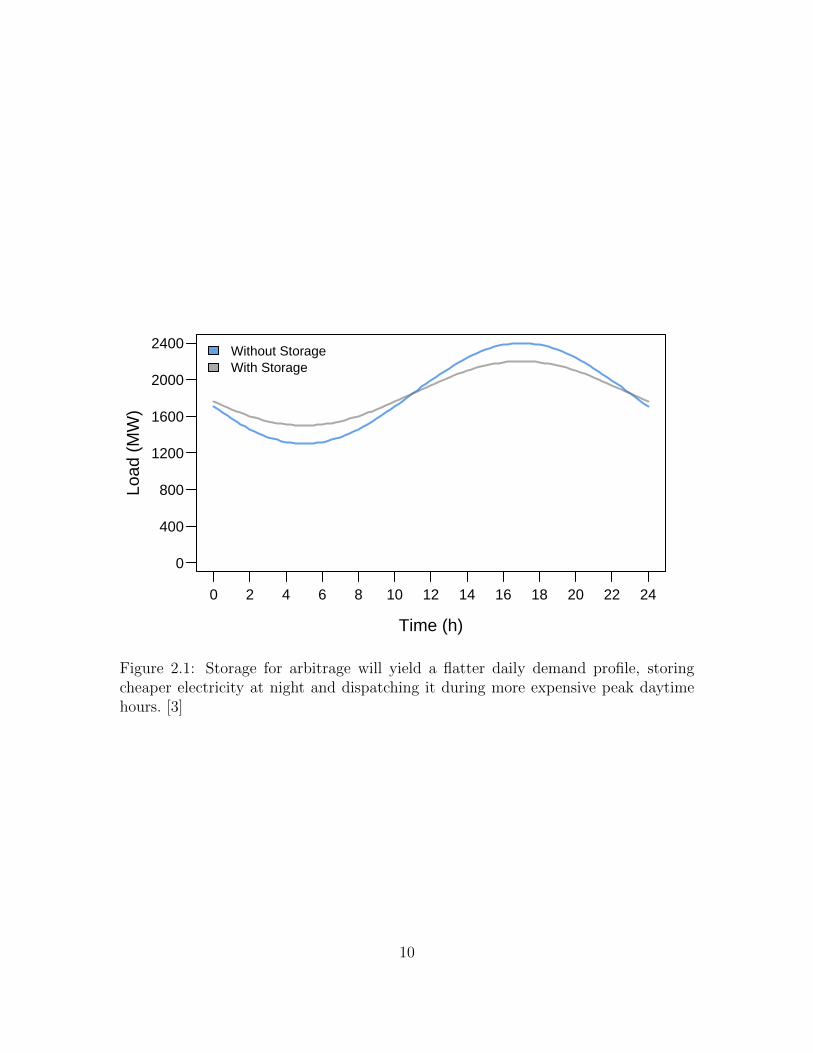
2.1 Storage for arbitrage will yield a flatter daily demand profile, storingcheaper electricity at night and dispatching it during more expensivepeak daytime hours. . . . . . . . . . . . . . . . . . . . . . . . . . . . 10
2.2 The estimated levelized costs of energy storage for 10 hour arbitrage(load shifting) are quite high. With computational studies, it maybe revealed, however, that these costs are outweighed by the benefitsoffered by energy storage. . . . . . . . . . . . . . . . . . . . . . . . . 13
2.3 Denmark increased available thermal generation from 1985 (L) to 2008(R) using mostly small, flexible and efficient combined heat and power(CHP) facilities. This development was a key component in their planto pursue aggressive wind generation growth. . . . . . . . . . . . . . . 15
3.1 In a scenario tree, the number of nodes, and hence, number of paths,increases exponentially as the depth of the tree increases. . . . . . . . 30
4.1 Nearly all of Austin Energy’s planned generation growth by 2020 willbe from renewable sources. . . . . . . . . . . . . . . . . . . . . . . . . 47
4.2 Decker Power Plant unit 1 CO2 emissions are modeled as proportionalto generator load (MW), a reasonable approximation that avoids in-troducing non-linearities to the model. . . . . . . . . . . . . . . . . . 48
5.1 Typical dispatch for a July 2020 day requires dialing back or shuttingdown inexpensive units at night and the use of older, dirtier generatorsto meet peak demand. . . . . . . . . . . . . . . . . . . . . . . . . . . 71
5.2 Dispatch with available storage in a July 2020 day meets peak demandusing wind energy available at night, avoiding the use of expensive anddirty generators and peaking units. . . . . . . . . . . . . . . . . . . . 74
5.3 In a November 2020 day, as with most winter and spring months inTexas, demand can be served almost entirely by baseload generationand renewables because variations during the day are limited. . . . . 76
5.4 As with the November 2020 scenario without storage, demand varieslittle throughout the day and is served by inexpensive generators, yield-ing minimal opportunity for benefit from energy storage availability. 77
5.5 Demand during winter months, as in February 2020, can be servedentirely by renewables and baseload generators in great part becauseof significant wind availability during these months. . . . . . . . . . 79
5.6 In the modeled February 2020 day, frequent ramping of some genera-tors appears, as in several other dispatch results with storage, likely aconsequence of the use of linear marginal costs for these results. . . . 80
xii

5.7 In most months, the availability of energy storage maximizes the dis-patch of inexpensive generators by shaping wind output. . . . . . . . 82
5.8 Benefits from the availability of energy storage scale roughly with max-imum allocation of storage. . . . . . . . . . . . . . . . . . . . . . . . 84
5.9 With a rolling planning solution method, the portion of the modelsolved as a full mixed-integer program is limited to a section of the fullstudy length to shorten solution times. . . . . . . . . . . . . . . . . . 86
5.10 As in earlier results, the availability of energy storage improves dispatchof inexpensive generators by shaping renewables availability. . . . . . 87
5.11 Energy storage flattens demand significantly throughout the year, andas shown in the histogram in the right panel, storage thus reducesthe number of hours of peak generation and the magnitude of peakrequirements while also increasing demand during the lowest few hoursof the year. Average load and standard deviation for each of these casesare summarized in table 5.3. . . . . . . . . . . . . . . . . . . . . . . 89
5.12 With the presence of CAES, the discrete scenario results show not onlya concentration of load levels to be served, as in figure 5.11, but also asmall overall reduction in load. . . . . . . . . . . . . . . . . . . . . . 90
5.13 With limited storage available, minimal reshaping of demand occurs,using storage to shift only the most expensive hours of the year, max-imizing the benefit of what storage is available. . . . . . . . . . . . . 91
5.14 While there is no clear bias towards storage in one period or anotherwhen quantities or model length are limiting factors, when energy stor-age quantities are unlimited, storage is concentrated primarily in thewinter and spring months, when stored energy is the cheapest. It islikely that the difference between generic and discrete storage behaviorin the final months of the year is a consequence of limiting constraintsin the discrete storage scenario. . . . . . . . . . . . . . . . . . . . . . 94
5.15 As CO2 prices increase, dispatch changes to use natural gas generatorsinstead of coal power plants. Since natural gas facilities are much moreflexible in their operation, less storage is required to achieve the samelevel of system flexibility. . . . . . . . . . . . . . . . . . . . . . . . . 100
5.16 Similar to CO2 prices, as NOx prices increase, dispatch shifts towardincreased use of natural gas generators, while storage changes to pro-vide needed system resilience. . . . . . . . . . . . . . . . . . . . . . . 101
xiii

Chapter 1
Introduction
Many utilities plan to significantly expand the portion of their total gener-
ation from wind, solar photovoltaics and concentrating solar power, alongside the
introduction of ‘smart grid’ technologies. Renewable power sources offer domestic
energy security and reduced carbon emissions, but their intermittency complicates
utility management and might limit the degree to which they can be deployed on the
grid. This intermittency, as well as unpredictability of customer demand, is currently
managed by operating primary fossil fuel generators at part-load, providing “spin-
ning reserve,” with fleets of fast-response gas turbines or diesel generators to relieve
spinning reserve providers. Revising this operational approach with the availability
of electrical energy storage could boost efficiency and provide more rapid responses
to interruptions. While the integration of renewable energy sources is typically one
of the key goals of the smart grid, other goals include greater system resiliency and
reliability, better utilization of existing non-renewable generating units and increased
customer participation, including demand-side management (DSM) through smart
metering and smart appliances. Energy storage might be able to improve outcomes
for all these objectives. Storage can also be used for arbitrage, which affects prices
and could have significant effects on customer energy conservation incentives.
To examine the potential benefits of energy storage, a novel unit commitment
model that captures storage attributes is developed. This modeling approach will
yield a structure that can be adapted to a variety of thermal generator and storage
1

constraints, as well as any meaningful set of generators and demand. The city of
Austin serves as the test region for the development of this model. Austin Energy
has generously provided data about historical dispatch and power plant operational
characteristics that fill critical roles in the structure of the model. Beyond these
data, Austin Energy serves as an appropriate initial case for model testing. They are
currently proceeding with the introduction of a wide range of smart grid technologies
to improve system awareness and operations. They also have aggressive demand-side
management programs to help reduce increases in peak demand into the future and
to increase market penetration of smart appliances to be able to attenuate demand
during peak periods. Further, the utility, in conjunction with the city, has committed
to an ambitious schedule for renewable energy introductions, with plans to obtain
30-35% of their electricity from renewable sources by 2020. More than 70% of the
renewable generation contracted to meet this target will be from wind energy, meaning
that by 2020, more than 20% of Austin Energy’s generation will be from wind.
Given the Austin Energy’s profile, energy storage could provide significant
operational value to them — firming and shaping renewable generation, providing
lower marginal cost generation during peak hours and reducing emissions compared
to fossil fueled backup generation, but the use of storage for these applications is not
well understood. The unit commitment model developed in this work is designed
to determine the optimal level of energy storage that will minimize operating costs.
Modeling capital costs through levelized cost of energy (LCOE) or another economic
metric would improve storage portfolio allocation as compared to examining only
operational costs by capturing the primary costs associated with storage. Unfortu-
nately, including storage capital costs would require knowledge about capital costs
and financing of existing plants owned by Austin Energy. Since these data are not
available, capital costs must be excluded from the model and are instead examined
2

with the model results instead of being captured in the objective function. Scenarios
using this basic framework reveal trends across months of dispatch and those results
are compared with a year-long model run. Due to the computational cost of such long
analysis periods, only a few year-long scenarios are run. In these year-long cases, the
unit commitment framework is extended to perform optimal storage selection from a
limited set of storage types. Finally, the effect of emissions pricing schemes on energy
storage selection is explored. From the results of these scenarios, storage portfolios
and implementation guidelines are developed.
3

Chapter 2
Motivation
In the interest of moving towards the use of more renewable, domestic and
secure resources for electricity generation, and often to meet ambitious renewable
portfolio standards (table 2.1), many states are rapidly deploying wind and solar
generation assets. [1] These generators, especially wind facilities, have highly variable
outputs and must be sited where the relevant resource is most available, creating
capacity constraints and additional reliability challenges. [2] Currently, intermittency
from these sources is managed with fast-response natural gas or diesel generators. [3]
These generators could be replaced with energy storage, which offers lower marginal
costs, protection from volatile fuel prices, greater system resiliency and zero emissions.
With the complexity and requirements of the electric grid, however, it is not obvious
if energy storage will be able to deliver these benefits at a reasonable price. This work
explores existing electricity generation and distribution system and changes planned
to implement the smart grid to determine what role energy storage might have in
the future smart grid. While some studies have examined the effect of energy storage
for specific applications or the particular benefits of one type of energy storage, this
work will develop a model that determines the optimal allocation of storage based on
the city of Austin that can be adapted to any region of study and for any type(s) of
energy storage.
4
2.1 Energy Storage and the Smart Grid
Energy storage has been identified as a potential component of the future smart
grid, one significant enough that it is specifically identified in Title XIII of EISA
2007. [4] As part of its mandate in EISA 2007, DOE has qualitatively determined
what roles energy storage could fulfill in smart grid development plans. [4] Since one
of the primary motivations of the smart grid is to increase the utilization of existing
generation, transmission and distribution (T&D) resources, energy storage can be
placed at the site of intermittent generators such as wind farms, at choke points
in the distribution network, or at a substation to improve local power quality and
reliability. [2] Placing storage at these locations could allow deferment of some T&D
improvements or enable optimization of an improved T&D system.
In addition to improvements in resiliency that can enable increased renew-
able energy generation, the smart grid will also enable greater system efficiency. The
Electric Power Research Institute (EPRI) has found that rollout of smart grid tech-
nologies could yield a 4% reduction in energy use in 2030 as compared to a reference
case. [4] As a point of comparison, that would be roughly equivalent to eliminating
the emissions of 50 million cars. [5] Beyond the emissions impact, that translates to
a $20.4 billion in annual savings for utility customers nationwide. [4] With a more
robust and efficient system, and better knowledge and control of demand, it will be
easier for utilities to manage the integration of renewable energy sources that pro-
duce intermittent power. That will help states meet targets for renewable power
growth and minimize fuel consumption by reducing their dependence on natural gas
or diesel reserve generators and use of fossil fuel-based power plants. Energy stor-
age can also support requirements for reserve generation in place of fossil fuel-based
facilities, yielding zero emissions and, without fuel needs, lower operating costs.
5

Table 2.1: Twenty-six states have set renewable portfolio standards (RPS) definingthe percentage of total electricity that must be generated from renewable sources byset deadlines. [5]
State Amount (%) Year
Arizona 15 2025California 20 2010Colorado 20 2020Connecticut 23 2020District of Columbia 11 2022Delaware 20 2019Hawaii 20 2020Iowa 105 MW -Illinois 25 2025Massachusetts 4 2009Maryland 9.5 2022Maine 10 2017Minnesota 25 2025Montana 15 2015New Hampshire 16 2025New Jersey 22.5 2021New Mexico 20 2020Nevada 20 2015New York 24 2013North Carolina 12.5 2021Oregon 25 2025Pennsylvania 18 2020Rhode Island 15 2020Texas 5880 MW 2015Washington 15 2020Wisconsin 10 2015
6

Energy storage could also be beneficial for utilities that have renewable gen-
eration that is not well matched to peak demand times. For example, Texas has
the largest installed base of wind power in the United States, nearly all of which is
located in western Texas, away from the state’s population centers. [6] West Texas
wind power is at its peak during the middle of the night, when demand is lowest. [7]
While sometimes that energy might be needed to supplement base load power plants
to meet minimum demand, often wind generation must be accommodated by dialing
back base load generators. On summer days with high peak demand, though baseload
generators might not be fully dispatched at night, inefficient peaking generation is
required during the day to meet demand. If energy storage were available, excess
nighttime generation could be deferred to peak hours when it is more useful. Energy
storage for arbitrage of renewables, however, is not limited to inland wind generation.
All solar photovoltaics, regardless of the quality of the solar resource, generate less
power as the sun goes down, just as demand approaches its peak.
Demand response control can assist utilities when unexpected supply losses
occur or during periods of unprecedented demand. Utilities, (regional transmission
organizations) RTOs and (independent system operators) ISOs contract with cus-
tomers who can support power losses in their operations in exchange for compensa-
tion. If a system operator encounters an unexpected need for reserve power, they
may temporarily disconnect these contracted customers to restore reserve availability
until demand falls or additional generation comes online. [8] As an example, in Texas
on February 26, 2008, the Electric Reliability Council of Texas (ERCOT) region ex-
perienced a significant unexpected loss of wind power at the same time demand was
increasing. To compensate for the sudden loss of reserve power availability, ERCOT
used its demand response capability to cut power to several customers. This ac-
tion was sufficient to restore balance to the system and minimized the impact of the
7

power loss, preventing much larger scale brownouts or blackouts. [9] While demand
response is helpful in providing system resiliency, energy storage could provide elec-
tricity as quickly as demand response when needed, reducing or eliminating the need
to interrupt customers.
If storage is only used to provide ancillary services, it will not have the same
interaction with smart pricing and customer behavior because it will lack sufficient
capacity to affect prices. This use will, however, increase utilization of planned im-
provements to T&D infrastructure. While this application provides significant opera-
tional benefits, it is unlikely to provide significant diurnal storage for renewables that
are not well matched to demand. Utilities will not be able to realize the same fuel
savings as with storage for arbitrage, but they will be less reliant on demand response
contracts to ensure that they have sufficient flexibility in their system, which can yield
some long term cost reductions. Thus, there is likely still benefit in pursuing smaller
amounts of storage for ancillary services if large quantities of storage for arbitrage is
not an option.
Alternately, storage could be used for arbitrage, storing electricity when gener-
ation is cheaper and returning it to the grid when prices are higher (figure 2.1). This
implementation can benefit a utility by increasing the utilization of existing generat-
ing resources, storing excess generation at night and returning it to the grid during
higher value hours during the day, as discussed previously. Unfortunately, peak de-
mand reductions from customers through smart pricing programs implemented as
part of smart grid development could nullify the value of storage for arbitrage. Us-
ing storage for arbitrage could flatten the effective demand curve, illustrated by the
sine curves representing demand and storage-adjusted demand in figure 2.1. Reduc-
tions in effective peak demand will mean fewer expensive power plants will have to
8

be dispatched, reducing the cost of peak power and minimizing customer incentive
to change behavior. Alternately, if customers respond to price signals or use smart
appliances to curtail their use during peak hours, the potential benefit of storage for
arbitrage during the highest priced hours of the year might not be possible, since
those hours will not be nearly as expensive. Energy storage might be a far more
expensive way to reduce variations in demand, but if placed appropriately within
the T&D system, using storage for arbitrage also ensures that most or all renewable
energy generated will eventually be dispatched. Since renewable energy sources typ-
ically have extremely low operating costs, their increased availability will offset fuel
use associated with traditional generating plants, allowing utilities to realize signifi-
cant operating cost reductions. Ignoring capital costs, these savings will exceed those
associated with demand-side management like smart pricing and smart appliances.
Both potential savings and the need for energy storage will increase with increasing
installed renewable energy generation.
Various studies have made qualitative assessments of possible operational ben-
efits to energy storage availability on the electric grid, but few studies have attempted
to quantify the potential benefits or the amount of energy storage that is appropriate
to meet particular operational goals. As a result, there exists no generalized frame-
work in the literature that has been developed specifically for studying the effects
of energy storage on the grid. Analytical methods such as unit commitment that
might serve as suitable approaches for quantitative analysis of energy storage have
only seen recent study. This work thus seeks to develop these study methods toward
the development of a tool that will enable determination of an optimal allocation of
energy storage and what portfolio of storage technologies might be optimal to reduce
operating costs associated with thermal generator dispatch.
9
0 2 4 6 8 10 12 14 16 18 20 22 24
0
400
800
1200
1600
2000
2400
Time (h)
Load
(M
W)
Without StorageWith Storage
Figure 2.1: Storage for arbitrage will yield a flatter daily demand profile, storingcheaper electricity at night and dispatching it during more expensive peak daytimehours. [3]
10
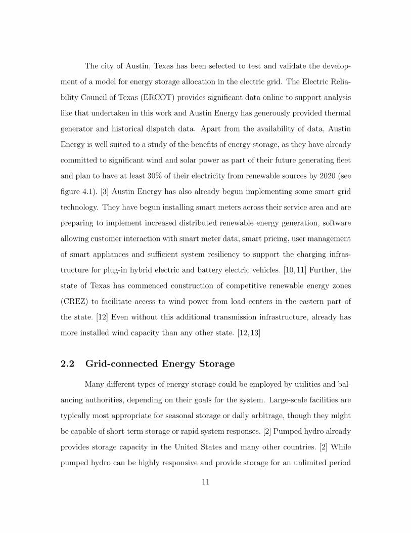
The city of Austin, Texas has been selected to test and validate the develop-
ment of a model for energy storage allocation in the electric grid. The Electric Relia-
bility Council of Texas (ERCOT) provides significant data online to support analysis
like that undertaken in this work and Austin Energy has generously provided thermal
generator and historical dispatch data. Apart from the availability of data, Austin
Energy is well suited to a study of the benefits of energy storage, as they have already
committed to significant wind and solar power as part of their future generating fleet
and plan to have at least 30% of their electricity from renewable sources by 2020 (see
figure 4.1). [3] Austin Energy has also already begun implementing some smart grid
technology. They have begun installing smart meters across their service area and are
preparing to implement increased distributed renewable energy generation, software
allowing customer interaction with smart meter data, smart pricing, user management
of smart appliances and sufficient system resiliency to support the charging infras-
tructure for plug-in hybrid electric and battery electric vehicles. [10, 11] Further, the
state of Texas has commenced construction of competitive renewable energy zones
(CREZ) to facilitate access to wind power from load centers in the eastern part of
the state. [12] Even without this additional transmission infrastructure, already has
more installed wind capacity than any other state. [12,13]
2.2 Grid-connected Energy Storage
Many different types of energy storage could be employed by utilities and bal-
ancing authorities, depending on their goals for the system. Large-scale facilities are
typically most appropriate for seasonal storage or daily arbitrage, though they might
be capable of short-term storage or rapid system responses. [2] Pumped hydro already
provides storage capacity in the United States and many other countries. [2] While
pumped hydro can be highly responsive and provide storage for an unlimited period
11

with minimal decay, it is only feasible in areas with sufficient water and elevation
changes. [2] Compressed air energy storage (CAES) stores air in underground caverns
and can provide storage on a similar scale, but few full-scale facilities have been con-
structed. [14] Also, CAES still requires fossil fuels, as all existing plants depend on
natural gas to heat the air as it expands out of the storage cavern, though researchers
are exploring solar thermal systems as a replacement for the natural gas. [14]
For shorter storage periods, as with ancillary service provision or to enable
more efficient T&D utilization, batteries might be the most appropriate storage type.
[2] Lead-acid batteries are a mature technology and relatively inexpensive, but they
can tolerate relatively few deep discharge cycles. Many utilities have tested lead-acid
battery systems, but none have pursued large-scale adoption of the technology. [15]
Over the long term, lead-acid batteries would become expensive because they require
frequent replacement as they lose capacity. [16] Lithium-ion batteries have become
popular in recent years for their high energy density and ability to withstand many
charge cycles. Unfortunately, lithium-ion technology is extremely expensive and, at
its current level of technological maturity, is better suited to applications where energy
density is more important, such as laptops and mobile phones. [16] High-temperature
sodium sulfur batteries (NaS) and redox flow batteries (RFB) both show promise for
utility scale applications, as they have the cycle life needed to withstand heavy use
for many years. [17] Because of only recent interest in energy storage for electric grid
applications, however, they are largely confined to specialized applications and pilot
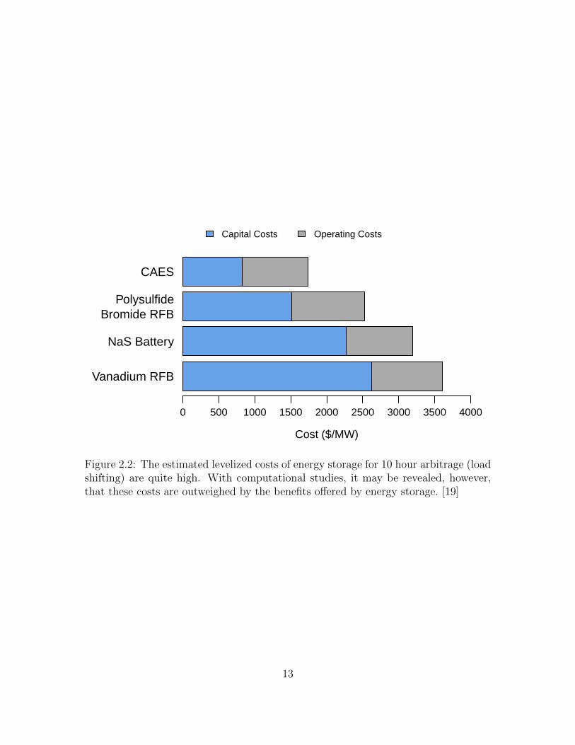
programs. [18] High costs plague all battery types, and are likely the largest barrier
to utility adoption of this storage type (figure 2.2).
A possible solution to the cost and implementation problems facing energy
storage in the smart grid is the use of batteries in plug-in hybrid electric vehicles
12
Vanadium RFB
NaS Battery
PolysulfideBromide RFB
CAES
Cost ($/MW)
0 500 1000 1500 2000 2500 3000 3500 4000
Capital Costs Operating Costs
Figure 2.2: The estimated levelized costs of energy storage for 10 hour arbitrage (loadshifting) are quite high. With computational studies, it may be revealed, however,that these costs are outweighed by the benefits offered by energy storage. [19]
13

(PHEVs). Utilities have envisioned that PHEV owners will plug their vehicles in at
night to charge and, with the installation of public charging stations, will also likely
be plugged in during the day while at work. [2] In this scenario, since PHEV batteries
will be available to the grid for most non-commute hours during the weekdays, PHEVs
can essentially be viewed as energy storage for the cost of public charging points. [2]
Encouraging or requiring PHEV owners to participate in a program that uses the
batteries in their car in this way will require a significant shift in the way they interact
with their utility. Information regarding the utility’s and owner’s plans for how the
car’s batteries are used must be coordinated if each is to get what they want out of
the car. Further, the utility will have to provide some incentive for PHEV owners
to participate in such a program, as the utility’s use of the battery will probably
shorten its life and occasionally make it unavailable to the owner. [2] Since there are
few battery electric vehicles (BEVs) and PHEVs on the road today, it is difficult to
predict their popularity and how owners will use them. The logistics associated with
utilities sharing battery use with vehicle owners will, however, present a significant
challenge for utility system planning. [2]
2.3 Addressing Stochastic Renewable Generation in the Elec-tric Grid
Regardless of the integration challenges associated with PHEVs, it remains
unclear how or even whether energy storage is needed in the United States electric
grid. Though this work seeks to determine the optimal implementation of energy
storage, clearer qualitative trends might be apparent when examining the strategies
adopted by other nations that have already introduced significant renewable genera-
tion. There are several such countries that have significantly higher levels of installed
wind energy than the United States, which is highly variable, and hence, a driver
14

Figure 2.3: Denmark increased available thermal generation from 1985 (L) to 2008(R) using mostly small, flexible and efficient combined heat and power (CHP) facili-ties. This development was a key component in their plan to pursue aggressive windgeneration growth. [5]
15

for energy storage deployment. For example, 20% of Denmark’s generation mix is
wind energy. [20] That is planned to rise to 50% for all renewables, mostly wind,
by 2050. [21] Despite these ambitious targets, as shown in figure 2.3, Denmark does
not have domestic energy storage. They are able to avoid the expense of domestic
energy storage because of several key features of their electric generation and T&D
systems. As can be seen in figure 2.3, much of the power generated in the coun-
try is derived from small combined heat and power (CHP) facilities. These small
generating plants provide district heating to neighborhoods and also generate local
electricity. [20] These plants are new facilities that are efficient and responsive, so they
can be cycled throughout the day with minimal equipment reliability and performance
impacts. [21] Figure 2.3 also shows the geographic diversity of wind generation facil-
ities in Denmark, which ensures unexpected weather patterns are unlikely to affect
many locations at once. The use of offshore and onshore wind also provides further
balance, as weather conditions often differ between those locations. [21] Denmark
exploits its extensive interconnects with neighboring countries Germany, Sweden and
Norway to balance power generation. [20] Through these interconnects, they can take
advantage of pumped hydro energy storage in Norway and Sweden. [21] Collectively,
these features of their generation system provide the stability needed to extensively
integrate wind power.
Ireland is less ambitious than Denmark in its wind integration plans, but
has set goals similar to many US states RPS’ standards, summarized in table 2.1.
[22] Ireland plans to generate 20% of its power from wind by 2020. [23] Because of
its expense, Irish researchers have sought to avoid the need for energy storage. [22]
Notably, Ireland has only one small 400 MW high voltage DC interconnect with
Scotland [23] and it cannot be used to provide real-time support for sudden losses of
wind power. [22] As a point of reference for the interconnection, the Irish system is
16
nominally 9600 MW. [22] Ireland has a diverse group of flexible generating facilities,
much like Denmark, which help it cope with increasing wind power installations. [22]
Ireland is also aided by a diversity of wind power generation locations, which will
not all be affected simultaneously by changes in weather. [23] To counteract the
lack of storage, researchers have already explored optimization methods that exploit
Ireland’s flexible generation fleet and improved T&D infrastructure to ensure that
the government’s 20% wind power goal can be reached without the use of energy
storage. [22] This approach, however, yields a measurable emissions penalty over the
use of energy storage for ancillary services. [22]
Because the United States electric grid lacks some of the features of those in
Denmark and Ireland, it appears that similar wind energy penetration levels can be
reached without energy storage or significant emissions and operational cost conse-
quences. Although smart grid improvements to T&D infrastructure will help support
the increased presence of renewable energy generation, the national generation fleet
has not benefited from recent construction of many efficient, flexible generating units
as in Denmark. [3] The Irish system uses inefficient gas turbines to provide ancil-
lary services and accepts the environmental consequences of such an approach, while
Denmark depends on the availability of pumped hydro storage from Scandinavia.
American utilities could expand installation of peaking generating units like in Ire-
land, but domestic utilities might wish to retain the emissions benefits associated
with renewable generation even when those resources are not available. The optimal
quantities, locations and types of storage to use cannot be known without further
analysis. Given qualitative evidence of operational benefit, independent system oper-
ators (ISOs) are nonetheless interested in proceeding with energy storage testing [1].
Unfortunately, with sub-optimal implementation strategies, system operators and
utilities might determine that their results do not justify the cost. [2]
17

Apart from energy storage, smart grid technologies promise many operational
advantages for all organizations responsible for ensuring reliable, consistent power
delivery in the United States. Planned improvements to T&D infrastructure and
smart devices that enable customer interaction and increase awareness of their power
consumption will enable more dependable, secure and efficient power generation and
delivery. They will also enable more effective utilization of existing generation re-
sources and increased integration of new renewable generation sources. While these
advantages are well established, the optimal utilization of energy storage requires
significant further study. In particular, researchers must determine what parameters
determine when energy storage becomes a requirement for a given region, how much
storage should be used and where that storage should be placed. Additionally, utili-
ties will be interested in the potential for cost reductions associated with storage for
arbitrage or alternately, at what capital cost threshold energy storage for arbitrage
becomes a good investment. A modeling approach that will explore the potential
benefits and characterize the optimal allocation of energy storage will be revealed in
subsequent chapters.
18
Chapter 3
Unit Commitment Modeling Theory
3.1 Unit Commitment Modeling for Future Scenarios withEnergy Storage
Unit commitment for an electricity generation system combines optimal eco-
nomic dispatch with forward-looking generator startup and shutdown to determine
which electricity generating units should be operating and at what level (in MW) for
every time step in a model. [24] Economic dispatch is the allocation of power from
each unit in a utility’s fleet of generators to minimize cost, maximize profit or achieve
some other operational objective(s) and occurs at each time step during the modeled
period. [24] Unit commitment is a common approach for electric power generator
scheduling [25], and basic models can serve as a foundation for exploring a variety of
specific system interactions and provide valuable future planning insight for system
operators, independent power producers, electric utilities and other market partici-
pants. [26] For example, unit commitment models can enable study of the effects of
deregulation or market restructuring, the introduction of new markets (e.g., a sepa-
rate market for ancillary services) or market rules, other market design changes, or
prediction of bidding strategies of participants in day-ahead and balancing markets
(as in ERCOT or other ISO systems). [27]
Other researchers have already applied unit commitment to study the effect of
energy storage on dispatch and the operation of generation systems, but their interests
have primarily focused on pairing an energy storage device with wind generation
19

to address intermittency or to explore the potential benefits of using PHEVs for
energy storage. [7, 28–30] This study applies unit commitment more broadly to the
allocation of energy storage, as opposed to specifically improving the performance of a
renewable generating facility or studying the effect of only one type of energy storage.
Austin Energy plans to introduce a sizable fleet of renewable generation, particularly
wind power, in the next decade. Significant emissions reductions, capacity factor
improvements and potential reductions in operating costs might be gained with the
availability of energy storage, but these benefits are unknown and existing studies do
not quantify overall improvements in system operation with energy storage. As unit
commitment methods are useful for studying future operational scenarios, they are
applied here to the exploration of the role energy storage could provide as part of
Austin Energy’s future generation plans.
While unit commitment is a well-established method for modeling electric
power generation systems and provides a suitable foundation for modeling future
scenarios, some limitations arise when examining energy storage. The ability of a
unit commitment model to predict the operation of some future generation assets or
the impact of a change in market rules is dependent on the selection of an appropriate
model and time step length. If careful consideration is not given at this stage, the
model’s results might give a solution implied by the selected time scales. For example,
if a model intended to examine some transient behavior has time steps that are too
long, it might fail to capture the feature of interest, giving results suggesting the
phenomenon does not occur or is insignificant. While this problem might appear
easily avoided by using appropriately short time steps, computational constraints
might limit the feasible number of time steps if the model length is many orders of
magnitude larger than the step. At the same time, some models might require long
time horizons to capture variations in demand or renewable resource availability over
20
seasonal time scales.
A unit commitment model could have a time horizon of only 24 hours or as
long as is desired for planning purposes, and the modeled period can be broken into
as many segments as is appropriate for the goals of the model. Typically, shorter
time steps are appropriate for examining impacts on system reliability, while longer
time steps are best for long-term planning. For a given model length, shorter time
steps increase computational cost significantly and yield minimal benefit in generator
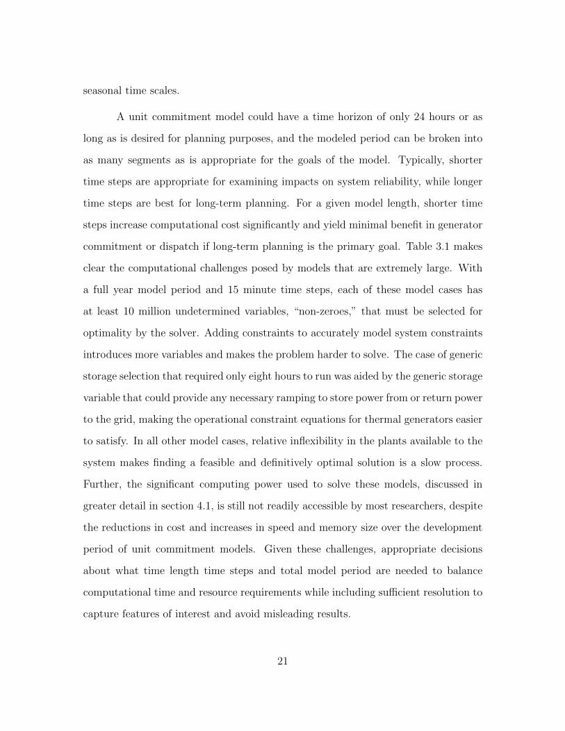
commitment or dispatch if long-term planning is the primary goal. Table 3.1 makes
clear the computational challenges posed by models that are extremely large. With
a full year model period and 15 minute time steps, each of these model cases has
at least 10 million undetermined variables, “non-zeroes,” that must be selected for
optimality by the solver. Adding constraints to accurately model system constraints
introduces more variables and makes the problem harder to solve. The case of generic
storage selection that required only eight hours to run was aided by the generic storage
variable that could provide any necessary ramping to store power from or return power
to the grid, making the operational constraint equations for thermal generators easier
to satisfy. In all other model cases, relative inflexibility in the plants available to the
system makes finding a feasible and definitively optimal solution is a slow process.
Further, the significant computing power used to solve these models, discussed in
greater detail in section 4.1, is still not readily accessible by most researchers, despite
the reductions in cost and increases in speed and memory size over the development
period of unit commitment models. Given these challenges, appropriate decisions
about what time length time steps and total model period are needed to balance
computational time and resource requirements while including sufficient resolution to
capture features of interest and avoid misleading results.
21

Tab
le3.
1:P
aram
eter
san
dop
tion
sap
plied
for
each
model
run
typic
ally
sugg
est
model
runti
mes
,w
her
efu
llye
ar(F
Y)
model
sre
quir
esi
gnifi
cantl
ylo
nge
rti
mes
than
singl
eday
model
s,ev
enw
ith
acce
ssto
grea
ter
com
puta
tion
alre
sourc
es.
(Furt
her
info
rmat
ion
rega
rdin
gth
edet
ails
ofea
chm
odel
run
isgi
ven
inA
pp
endix
A)
Model
Cas
eSol
uti
onT
ime
Rol
ling
Pla
nnin
g?N
on-z
eroes
Iter
atio
ns
Opti
mal
ity
Cri
teri
on(%
)T
ime
Lim
it(s
)It
erat
ion
Lim
it
2020
Mon
ths
3m�
No
29,1
5315
00�
0.1
1000
2,00
0,00
0
2008
w/o
Sto
rage
,F
Y†
unk.
Yes
nz
iter
0.00
177
7,60
01,
000,
000,
000
2020
w/o
Sto
rage
,F
Y†
51h,
49m
Yes
10,7
16,3
3132
8,59
00.
001
777,
600
1,00
0,00
0,00
0
2020
w/
Sto
rage
,F
Y‡
8h,
12m
No
11,5
94,7
1990
0,85
00.
0001
777,
600
1,00
0,00
0,00
0
2020
w/
Dis
cret
e,F
Y†
98h,
16m
No
13,7
02,8
832,
207,
528
0.00
1*25
9,20
01,
000,
000,
000
2020
w/
Lim
ited
,F
Y†
4h21
mN
o13
,702
,883
1,76
3,05
10.
0135
0,00
01,
000,
000,
000
2020
w/
Em
issi
ons,
FY†
72h–2
17h
No
11,8
40,6
711,
100,
000–
3,50
0,00
0*0.
001
777,
600
1,00
0,00
0,00
0
†T
his
case
was
run
wit
hG
AM
S/C
PL
EX
op
tion
sn
odefi
lein
dat
3an
dw
ork
mem
of
8192
meg
abyte
s.S
eeA
pp
end
ixA
for
det
ail
s.‡
Th
isca
sew
asru
nw
ith
work
mem
of10
24
meg
abyte
s.S
eeA
pp
end
ixA
for
det
ail
s.*
Did
not
full
yco
nver
ged
ue
tore
sou
rce
lim
its.
�A
pp
roxim
ate
valu
es
22

Given the computational requirements associated with lengthy or large system
models, it might appear that applying a heuristic solution approach, one based on
typical historical generator dispatch, could serve as a simplified substitute for unit
commitment modeling. Such heuristic methods were popular when computational
resources were expensive and limited, but this approach dictates the solution space
and limits the ability of the user to capture any operational objective outside that
which defined the original heuristic. [31] With the availability of robust optimiza-
tion tools and solvers and ample computational capability, unit commitment enables
flexible modeling of a variety of scenarios without heuristics. [32] It also avoids the
presupposition that a modeled future scenario will operate in a manner consistent
with historical empirical data and reduces the risk that assumptions used to build a
heuristic will unintentionally promote particular outcomes.
While, in theory, heuristics could be used to solve unit commitment problems,
as discussed previously, applying heuristics to these systems might yield misleading
solutions. As a result, optimization techniques are well-suited to unit commitment.
Unit commitment could be considered part of a class of problems that involve system
scheduling and planning or resource allocation. While optimization has been used to
solve unit commitment problems with varying levels of success since at least a half
century ago [24], similar problems have been studied in conjunction with optimization
methods for at least as long, providing additional opportunities for the discovery of
improved solution methods. Many practical problems have similar formulations to
unit commitment problems for power generation, such as river flow management
systems or networks, traffic flow study, manufacturing plant operations and product
distribution systems. As a result, there exists a rich operations research literature on
these problems. [25] In some cases, this work might even be combined, where river
flow management and significant quantities of hydro generation (as in the northwest
23
United States or Brazil) might be studied with unit commitment of other generators
to model a complete power generation system. [32] These previous studies provide
meaningful guidance to future work studying novel systems with unit commitment.
3.2 Previous Unit Commitment Modeling Efforts
Modeling of power generation systems using a unit commitment approach be-
gan more than 50 years ago, around the time mathematical computing resources
became available to a limited number of large research institutions. [33] Because of
the potential complexity inherent in meaningful modeling of any sizable fleet of gener-
ating units over a time horizon of more than a few hours, the availability of computers
was pivotal to the use of unit commitment methods. [33] Extremely expensive com-
puting resources with limited capabilities significantly limited the size and complexity
of viable models. [33] Typically, the method of Lagrange multipliers or Lagrangian
relaxation was used to reduce computational requirements. [33] Lagrangian relaxation
is a necessary condition of optimality that moves inequality constraints into the ob-
jective function, creating a new objective that acts as a lower bound on the solution
space of the original problem. [33] Despite extraordinary computational limitations,
development of unit commitment models were immediately undertaken to study op-
timal electricity generation systems because of the staggering cost savings that could
be derived from even small improvements in dispatch decisions. [24] These historical
developments form the foundation for the unit commitment modeling formulation
presented in section 4.3.
Muckstadt and Koenig [24] developed a relatively complete unit commitment
model that captures many of the constraints required to model thermal generators.
Their model includes production, startup and shutdown costs, reserve allocation,
24

as well as transmission constraints, included through quantification of transmission
limitations as incremental production costs so that a new cost type need not be
introduced. [24] While computational limitations constrained their ability to model
extended periods, the authors identified 24 hours as the required minimum period to
capture the changes in unit commitment between low demand early morning hours
and peak demand during the late afternoon. [24] They also chose to attempt modeling
in two hour increments, more than previous authors had succeeded in modeling. [24]
To model what was at the time a very large system, Muckstadt and Koenig
employed a novel approach to Lagrangian relaxation by applying the relaxation across
generators. Previous work from Muckstadt and other authors avoided decomposition
using Lagrangian relaxation, which sometimes resulted in algorithms that were un-
able to find feasible solutions, or applied decomposition across time steps, which made
finding a feasible solution challenging since the main motivation of unit commitment
is to reveal economic dispatch decisions made with respect to constraints across many
time steps. Applying optimal economic dispatch where discrete time steps are not
connected limits the model’s value by eliminating its ability to plan for future changes.
For example, as demand increases during daytime hours, additional generating units
might need to be brought online to meet future demand, but making these units
available at appropriate levels during rising demand might require bringing them on-
line before they are strictly needed. [24] To accommodate the initial activation of a
generating asset at its minimum load, other units might need to be dialed back from
optimal generating levels for a short period. Because performing economic dispatch at
discrete time steps does not capture planning that requires knowledge or forecasting
beyond the current time step, it cannot appropriately model commitment of thermal
generating units. [24] Though such an approach might provide computational cost
benefits, startup and shut down penalties, up and down ramp rates, and responsive
25

(spinning) reserve, which can only be included in full unit commitment models, are
important components of thermal generator operation and should not be ignored. [26]
Recognizing the importance of temporal constraints between time increments moti-
vated the authors’ approach of decomposition of generating units. The decomposed
subproblems were solved using dynamic programming, followed by a final branch-and-
bound method to yield the optimal feasible solution. While this simplifying solution
approach is not employed in models developed here, Muckstadt and Koenig’s recog-
nition of capturing constraints across time periods remains an important component
of unit commitment modeling. [34,35]
Even with these aggressive decomposition approaches, limited computational
power meant the use of mixed-integer programs (MIP) for unit commitment was still
out of reach for problems of a meaningful size — more than about 12 time steps
and 15 generating units. [24] Further, for problems with more than ten generators
and ten time steps, convergence to a value of less than 0.5% was not achievable with
reasonable computational expense. [24] Despite these limitations, for more than two
subsequent decades, while computational resources remained a binding constraint,
the approach applied here defined the mathematical decomposition methods applied
to unit commitment models. [24]
Subsequent work on unit commitment models applied the basic decomposition
approach developed by Muckstadt and Koenig but modified the approach to empha-
size a feature or capture a particular constraint of interest. Zhuang and Galiana [35]
developed a heuristic approach to fully capture all types of reserve power require-
ments for a typical system. To explore the effect of ramp rates, not discussed by
Muckstadt and Koenig as an operating constraint on thermal generators, Wang and
Shahidehpour departed from Muckstadt and Koenig’s solution approach, favoring a
26

novel artificial neural networks approach to find optimal but infeasible solutions and
then using heuristics to search locally for a feasible solution. [31] With an improved
decomposition approach and greater computing power, Bard [34] was able to examine
a much larger problem than Muckstadt and Koenig, up to 100 generators and 48 time
periods, without the need for a branch-and-bound approach to find a feasible result
from the dual problem. He also examined the effect of including generator ramping
constraints. [34]
Following the work of these and other authors, Baldick [26] developed a unit
commitment approach capturing in one model all of the constraints relevant to the
unit commitment problem. Like many of his predecessors, Baldick continued to use
the solution approach originally proposed by Muckstadt and Koenig while also lever-
aging lessons from the literature to structure the problem and decomposition to speed
solution times. [26] The emphasis of this paper, however, was on the development of
a generalized unit commitment approach, including thermal generator startup and
shutdown costs, minimum up and down times, ramp rate limits, reserve power avail-
ability, fuel and energy limits, power flow limits, line flow (transmission) constraints
and voltage requirements, along with the scheduling of hydroelectric generation. [26]
Since this formulation captures most significant operational constraints, it largely
parallels the model developed in section 4.3. The inclusion of hydroelectric genera-
tion in the unit commitment problem was an improvement specifically identified by
Muckstadt and Koenig for future workers. [24, 36] While the author still depends on
Lagrangian relaxation to find feasible solutions, sufficient computational resources
were available to solve a problem of reasonable size (10 generators and 24 periods)
with nearly all of these constraints included. [26] Further, the author indicates mod-
els that selectively exclude constraints will likely yield suboptimal solutions, though
the final model presented neglects power flow and voltage requirements. [26] Based
27

on this conclusion, the model presented here attempts to capture all major thermal
generator operational constraints.
Beyond these workers, despite the increasing availability of sufficient computa-
tional resources to solve full MIP models, capturing all operational limitations without
simplification or decomposition strategies, many authors continued to pursue alterna-
tive strategies, testing models with incomplete constraints. [25] While these research
pursuits often led to robust, efficient solution methods, the availability of greater
computing power has meant many of these approaches are no longer necessary and
their incomplete models are less than desirable. Baldick’s note to future researchers
regarding the problems with results from incomplete models did not halt their pro-
liferation and led to repetition of his admonition in later work. [26] Goransson and
Johansson identified several articles by other authors that ignored some constraints
in the interest of expediency. [20] Goransson and Johansson revealed that the inclu-
sion of minimum load level, startup time and startup costs yield a unit commitment
model that better predicts operating costs when compared to models excluding those
parameters. [20] In their study area, western Denmark, complete modeling of plant
operating constraints increases operating costs and emissions by as much as 5%, in
addition to increasing import and export quantities from neighboring countries. [20]
Following the contributions from and outcomes of these researchers’ work, here a MIP
model is developed that is as complete as is required to capture all costs relevant to an
electric utility, avoiding the explicit use of decomposition strategies and heuristics and
depending instead on the solver to select those strategies that will yield optimality
given the inclusion of all constraints.
28

3.3 Stochastic Programming and Unit Commitment
With the proliferation of powerful and inexpensive computing resources, unit
commitment models have continued to move toward greater accuracy, capturing all
readily modeled system capabilities and operational constraints. Now that large de-
terministic models, with hundreds of generators for thousands of time steps, can be
solved easily, interest has turned towards stochastic modeling of system components
formerly idealized as deterministic. The components of greatest interest are demand,
which was historically the sole major stochastic element in the electricity system mod-
els, and wind generation, which is subject to significant variability and is of recent
interest. As a result, a significant body of contemporary work on unit commitment
has applied stochastic programming methods to determine the effect that modeling
systems as stochastic instead of deterministic has on the response of that system. [37]
Stochastic programming could be important in creating a unit commitment model
of Austin Energy’s future generating mix since wind energy forms such a significant
component of the total generation mix, as shown in table 4.1. Further, using stochas-
tic programming to represent wind energy could increase the quantitative savings
from energy storage in the model results, as energy storage can serve to moderate
variability in the grid.
Many researchers have independently pursued the modeling of stochastic ele-
ments in unit commitment problems, leading to a variety of approaches to modeling
stochasticity, however, scenario-based methods appear to be preferred by most au-
thors. [22, 37, 38] Stochastic elements are typically modeled by generating scenario
trees, as in figure 3.1, based on historical data. Monte Carlo-based methods, such
as Markov chains, have been used by some authors to cope with large quantities of
historical data. [22] If scenario generation demands or historical data are more limited
29

Figure 3.1: In a scenario tree, the number of nodes, and hence, number of paths,increases exponentially as the depth of the tree increases. [39]
or the scenario tree is shallow, simpler methods may be employed. [38]
The method used to create scenarios in a structure such as figure 3.1 is con-
ceptually similar to that used by Watkins et al. [38] and Kracman et al. [40]; both
authors generate scenario trees based on historical inflow data for a watershed. The
number of branches from each node of the tree and the overall depth of the tree
were preselected by the researchers to manage tree size, and hence, computational
requirements. [38] These historical data were sorted by magnitude and then separated
into segments based on the number of branches from the first node. [40] Then, each
segment of data was again sorted by magnitude and split based on the predetermined
number of branches. This process continued until all the planned branches had been
filled. [40] With a completed tree, the authors assume the probability of every path
is equal. Approaches explored in [22, 41] may be applied to construction of these
30

scenario trees, where each terminal (leaf) node has a defined path to the root node
and each of those paths has a probability that can be estimated based on historical
data, rather than assuming all scenarios have equal probability.
Applying stochastic modeling of system elements requires restructuring of the
unit commitment model from a deterministic predecessor. If using a scenario tree,
model equations with the terms of interest (e.g. load, wind generation) must be
multiplied by a probability variable. The model is then solved as before, with the
probability and values of each path from the scenario tree inserted where appropri-
ate. Both Tuohy et al. [22] and Watkins et al. [38] show clear examples of where
these terms appear in unit commitment model equations. Unfortunately, while this
stochastic programming approach is easily implemented from a deterministic basis,
it presents a significant computational challenge. [22] If the formulation were solved
deterministically, it would be equivalent to solving the problem for one particular
scenario. [22] For every additional scenario, the model must be run again. [22] There
are some simplifications solvers can apply to reduce solution time once the problem
has been run once, but the additional computational time required for scenario tree-
based stochastic models is inevitably much greater than with equivalent deterministic
systems. [22]
Initial applications of stochastic programming to unit commitment focused
on demand, which has always been an only moderately predictable element utilities
accommodate in their generation planning. [42] Recent interest in reducing the envi-
ronmental impact of electricity generation has yielded extensions of these models to
capture stochastic sources of renewable power. [42] Tuohy et al. [22] built upon the
stochastic unit commitment model developed by Barth et al. [43] to model stochastic
load and wind generation. Both implemented rolling planning, where the probabil-
31

ity of a certain outcome increases as it approaches the present modeled time and
‘knowledge’ of that period improves. Pappala et al. [44] developed a similar model
using a particle swarm optimization-based scenario generation and artificial neural
network solution approach, similar to Shahidehpour and Wang [31], instead of the
more common scenario tree method. All three models were developed with an em-
phasis on determining the effects of significant wind penetration, greater than 20%
of total generation, on the operation of fossil fuel-based generating units in the sys-
tem. While it would appear that such an analysis would be of significant interest
here, compensating for the uncertainties associated with stochastic elements in a unit
commitment model increases the commitment of mid-merit and peaking generators.
This change in commitment requirements yields minimal benefit and required solu-
tion runtimes as long as eight days. [22] Pappala et al. found increases in predicted
operational costs and improvements in schedule quality based on increased system
resiliency of 2-4%. [44] In a similar study, Tuohy et al. found improvements of less
than 1%. [22] Despite contemporary availability of significant computational power
and the anticipated improvements in unit commitment and dispatch resiliency associ-
ated with stochastic modeling, the minimal improvement realized with these methods
does not appear to merit required computational resources.
3.4 Grid-connected Energy Storage
With the rapid growth of stochastic renewable energy generation in the past
decade, energy system modeling efforts have focused not only on applying stochastic
programming methods to capture those effects but also on modeling the potential
benefit of energy storage for compensation. Some analyses of energy storage forgo
the creation of a complete unit commitment model, using commercially available
software packages or readily available data provided by ISOs or other market opera-
32

tors. [7, 45–48] Because the utilization of energy storage in the electric grid has only
received recent attention and no public, widely available empirical data exist from
what limited energy storage tests have taken place in the United States, potential
applications, siting and of energy storage are only partially characterized. Further, a
wide range of analytical approaches from various authors have provided meaningful
results for a specific circumstance of interest. Thus, these studies have often intro-
duced approaches that are not easily replicated and might only be useful in examining
the particular storage function or capability of interest to the authors. As a result,
there remain many opportunities to characterize the potential applications and ben-
efits, if they exist, of energy storage in the electric grid. The study performed here
will apply established unit commitment approaches for thermal generation previously
explored in section 3.2 to reveal the optimal use of energy storage.
Early studies of energy storage were concerned primarily with role of storage in
the market, examining the functions it serves best — ancillary services and regulation
or arbitrage — while ignoring costs, and in some studies, determining when it is
cost effective to provide that service. Since cost is a primary barrier to storage
implementation, its best function is of significant interest, as the appropriate use of
storage will determine its future implementation. Without any prior study of which
storage technologies might provide the greatest benefit, analysis of many available
technologies revealed that storage for ancillary services was likely cost effective, given
the low cost of small quantities of storage and the sometimes high prices paid for
these services. [45] Primarily as a result of high storage capital costs across all major
technologies, early analysis of arbitrage did not appear cost effective with minimal
wind generation and low electricity prices. [45] At the same time, several authors
pointed to arbitrage as a much more beneficial function for storage, particularly with
high levels (greater than 20%) of wind generation or high energy prices, if capital
33

costs could be managed. [45,46,49] Studies that ignored storage capital costs favored
arbitrage. [46] A few have noted that optimal application of storage for arbitrage
would be impossible for an operator to achieve in a real electricity market because
it is impossible to predict future prices, however, Lund et al. [46] propose a few
strategies to achieve near-optimal results. It should be noted that these methods
could be implemented by a utility operating energy storage for aribtrage, but further
exploration of computational approaches to accurately predict future electricity prices
are beyond the scope of this work.
Beyond this early work, the primary storage application of interest to most
authors was price arbitrage, as larger storage facilities can likely also provide ancil-
lary services. Small-device arbitrage, where energy storage acts as a price-taker and
takes advantage of the large price differences between nighttime and peak periods,
as mentioned previously, could be profitable if future market conditions change. [47]
Increasing quantities of storage will diminish the difference between peak and off-peak
prices, reducing the marginal benefit to the operator of further increases in storage
availability. Large quantities of storage might be able to provide other benefits, such
as improved utilization of existing T&D resources, congestion management and de-
ferral of capital investments in generation and T&D. [48] Regardless of the size of
available storage, round-trip efficiency has a significant impact on the value of stor-
age. Compromising efficiency to reduce costs is of significant detriment to the value
of the stored energy and thus, of the arbitrage effectiveness. [47, 48]
In large quantities, energy storage could provide sufficient capacity to make
wind or other renewable generation into a dispatchable or “firm” resource, much like
a thermal generator. With current energy and storage prices, such large quantities of
storage are cost-prohibitive. In the future, however, market changes might promote
34

such a use of energy storage. Without carbon pricing, comparing the generation of
baseload power from natural gas, wind with natural gas support or wind with CAES
support, the combination of wind and CAES has the highest levelized cost. At carbon
prices in excess of $35/ton of carbon (not CO2), Greenblatt et al. [50] find that wind
and CAES combined generation is price competitive with coal generation. If other
energy prices increase or the cost of wind turbines and CAES facilities decrease, lower
carbon prices might yield a similar result. [50] Further, the presence of energy storage
transforms wind into a dispatchable resource and enables wind capacity factors of
greater than 80% by storing wind when it cannot be used and dispatching it when
needed. [50] For baseload generation, this approach promotes the construction of
wind generation and energy storage far beyond the capacity of available transmission
to ensure continuous use of all transmission capacity. [50] A baseload generation
application of wind power requires the collocation of wind and storage, but the optimal
siting of storage for non-baseload power was not addressed by Greenblatt et al. [50]
The optimal location of storage is of significant interest, as storage might be
better able to make renewable generation dispatchable when it is collocated with the
generation instead of being located at the load, as some authors (and this work) as-
sume will occur. [50] While early studies identified binding transmission constraints as
a potential problem with energy storage collocated with wind generation, few studies
have determined what effect transmission constraints and other system limitations
would have on the sizing and effectiveness of storage. [45] In contrast to Greenblatt
et al. [50], where the author’s objective was to provide firm wind for baseload power,
Denholm and Sioshansi [7] find that when collocating storage with wind, less than
25% of the wind farm’s capacity should be provided as storage. Broadly, improved
utilization of transmission capacity at high transmission costs might warrant energy
storage, but sizing and revenue might vary depending on the particular transmission
35
corridor. [7] In examining the arbitrage value of storage specifically, the locational
value of storage at various nodes in the Pennsylvania-New Jersey-Maryland intercon-
nection (PJM) were found to vary by as much as 25%, dependent on transmission
constraints, storage efficiency and energy prices. Storage participation in the ancil-
lary services market, while currently restricted in PJM, could increase the variation
and magnitude of revenue from energy storage significantly. [48]
Beyond conventional stationary energy storage, PHEVs have recently been
of significant interest because, if popular, they are a possible source of free or low-
cost energy storage for regulation and arbitrage. Depending on the primary focus of
the study — consumers or operators and minimizing emissions, profits or costs —
conclusions about the value of vehicle-to-grid (V2G) services from PHEVs vary widely.
[28–30] Sioshansi and Denholm [28] created a unit commitment model of ERCOT to
focus on the emissions benefits associated with V2G services. For simplification,
they assumed PHEVs would always be plugged in for hour increments starting on
the hour and that PHEVs would always be plugged in when not in use. These
assumptions enable PHEV participation in ancillary services markets, which might
be of significant value during peak hours. Other studies have revealed that the use
of LiFePO4 batteries, as in PHEVs, for V2G energy results in less than half the
capacity loss of driving and that there is minimal capacity loss associated with deep
discharge. [29] These results suggest the use of PHEV batteries for ancillary services
instead of arbitrage will not extend battery lifetimes but might limit profits. Further,
Peterson et al. [30] found that it is unlikely that PHEVs can be used for ancillary
services since their availability during peak hours, when ancillary service market prices
are highest, will be limited. The authors estimate that less than 5% of PHEVs will
likely be available for ancillary services.
36
If the use of PHEVs for arbitrage grows, as in Sioshansi et al., the difference
between peak and off-peak prices will be limited and PHEVs participation in the
ancillary service market might be limited, the value of V2G services to vehicle owners
will be limited. [48] Assuming battery replacement costs are paid by the utility, annual
vehicle owner profits from V2G services will likely be around $200. If vehicle owners
are forced to provide V2G services by their utility at the owner’s expense, annual
profit will likely fall to less than $100 due to battery replacement costs. [29,30] These
results suggest that V2G incentives are too limited to promote widespread adoption.
The potential role of PHEVs on the grid, however, is examined here on a limited
basis.
37

Chapter 4
Unit Commitment Modeling with Storage
4.1 Methodology
As discussed in chapter 3, unit commitment methods have been applied by
many authors to explore the effects of modifications to the electric grid. [25] I will
examine the role energy storage can play in the electric grid to minimize total op-
erating costs and costs with respect to NOx and CO2 emissions, similar to models
developed by Sioshansi and Denholm [28] to study possible cost, reliability and emis-
sions benefits from PHEV V2G technology. This analysis uses a MIP approach, which
facilitates representation of complex thermal generator operational constraints, such
as minimum load level, startup costs and shutdown costs. It does not capture non-
linear heat rates or emissions characteristic of thermal generators. Modeling these
non-linearities is avoided because of the complexity they introduce.
In the early stages of model development, MATLAB was used with its opti-
mization toolbox. but due to toolbox limitations, MATLAB was ultimately replaced
with a more robust optimization program. MATLAB is fast and convenient when
solving linear programs (LPs) but, because of the way MATLAB functions handle
constraint data, the optimization functions were limited in their ability to model
semi-continuous, binary and integer variables. Since modern unit commitment mod-
els are almost exclusively MIPs, without additional third-party packages, MATLAB
could not handle realistic constraints on thermal generator operation. To overcome
these limits, the model was rewritten using the General Algebraic Modeling System
38

(GAMS), a program designed specifically for solving optimization problems. As will
be explored further in section 4.3, GAMS offers significant convenience by provid-
ing simple methods for the introduction of major model components — parameters,
vectors of operating constraints; and variables — and the declaration of equations
with straightforward, intuitive notation. GAMS transforms user inputs in this form
into the objective and constraint equations that an appropriate solver will accept as
inputs. This framework does not constrain the type of model to be solved, number
of constraints, length of time steps or total number of time steps.
Because GAMS is a well-established tool for optimization studies, for every
problem type, there exist several solvers that can be used. While many solvers are
available, it is outside of the scope of this work to explore the performance of each
one. Instead, I have chosen to employ CPLEX, a linear and mixed-integer program
solver developed by IBM ILOG that provided robust solutions for the MIP problems
solved here.
Initial work in MATLAB was performed using an Apple PowerBook G4 1.33
GHz with 2GB RAM running Mac OS X 10.5.7 and MATLAB R2009a. For prelimi-
nary implementation in GAMS, the only available license was for Microsoft Windows.
This initial work was performed on an Apple MacBook Pro 2.53 GHz Intel Core 2 Duo
with 4GB RAM running Mac OS X 10.6.3 and Windows 7 Professional running na-
tively in Apple Boot Camp or virtualized using VMware Fusion 3.0.2. Initial models
examined a 24-hour dispatch window in 15-minute time increments. Because GAMS
stores a significant portion of data for the solver in the computer’s physical memory
(RAM) to speed repeated computations, when the dispatch window was extended and
model functionality expanded, physical memory limits became a binding constraint
on model size. As a result, the model was slightly modified to run on The University
39

of Texas at Austin Mechanical Engineering department’s high performance comput-
ing (HPC) cluster. The HPC is a system of eleven rack-mounted Dell Poweredge 2950
workstations running Ubuntu Linux, each with two dual-core, hyper-threading 3.73
GHz Intel Xeon processors and 24 GB of shared RAM. The vast hard drive storage,
physical memory and processor power available on the HPC enabled problem sizes as
large as one year in 15-minute increments, or 35136 time steps. Even larger problems
could be solved if they were of interest, particularly with the use of more advanced
decomposition techniques, such as rolling planning. [22] Visualization of all results
were completed entirely on the Apple MacBook Pro in the Mac OS using R version
2.19 and the R GUI version 1.31. [51]
Initial models used to test the operation of new constraints studied only a 24-
hour dispatch window in 15-minute time increments. These preliminary results from
building the model in GAMS are presented in section 5.1. Once constraint equations
and output were tested in this arrangement, the model was changed to study dispatch
for a full year and, since GAMS is highly flexible, minimal modifications to GDX (a
proprietary input/output file format used by GAMS) files were the only changes
required. Major results presented in sections 5.2 and 5.3 examine a full year of
demand, as in Tuohy et al. [22] Modeling such a long time period ensures that seasonal
variations in the optimal allocation of energy storage will be fully characterized.
Because of the length of a full year unit commitment model, 15-minute time steps
are used for optimal economic dispatch to manage computational requirements. The
choice of time step size is extremely important. Time steps that are larger than a
few minutes might predispose the model to optimal outcomes that suggest storage
for arbitrage only, since temporal resolution is insufficient to capture ancillary service
provision. In its current form, the model can indicate whether and how much storage
can provide arbitrage benefit. Unfortunately, 15-minute time steps provide insufficient
40

resolution to model the use of storage to improve system reliability or provide ancillary
services, which are areas where storage has been predicted to be useful. [7, 28, 47]
Minute-by-minute demand and wind generation data would be required to study
the effect of energy storage on system reliability, but such a model for a full year
would be so large that it would be beyond the practical capabilities of even the best
commercial MIP solvers. As a result, longer time steps to enable modeling of a full
year period have been chosen in the interest of finding an optimal level of energy
storage for general system operation. It is likely that some limited regulation for
system reliability could nonetheless be provided by an arbitrage-optimized storage
system.
Early models, both those with 24-hour and full-year dispatch, used exclusively
marginal cost objective functions. These results are presented in sections 5.1 through
5.3. The last set, in section 5.3, includes emissions cost minimization objectives with
linear emissions rates and varying emissions prices. These approaches proceed toward
improving representation of real system constraints and limitations, where the final
set in section 5.3 represent some future scenario where emissions pricing might affect
dispatch decisions and economic value of storage. In unit commitment models like
these, profit maximization is a reasonable alternate approach for treating operating
costs. Such an approach, however, is avoided here. While the marginal cost for the
last (most expensive) unit dispatched could be used as a proxy for the market price
of electricity, enabling a profit maximization model, it would not necessarily provide
the most accurate representation of market prices in all time periods. Because the
ERCOT market, where prices are set for most of Texas, has a variety of generators,
the generators that are marginal (price-setting) from Austin Energy’s fleet for every
modeled time step might not closely represent the costs for ERCOT’s marginal gener-
ator(s). Further, during periods of scarcity, when limited excess capacity is available,
41

particularly during the early evening hours of the summer months, prices based on
marginal costs might fail to capture the effects of limited available capacity in the
system and might thus significantly underestimate market prices.
The selection of appropriate objective functions is critical to the value of results
generated by the model. Constraints governing the operation of thermal generators
are, however, also important to ensure that results that satisfy the objective are also
consistent with real system limitations. In the interest of modeling realistic thermal
generator limitations, the model developed here includes most of the critical elements
identified by Baldick [26] and often omitted by other authors. [25] Thermal genera-
tor constraints include up and down ramp rates (MW/min), minimum startup and
shutdown levels (MW), generator nameplate capacity (MW), startup costs, and pro-
vision of spinning reserves. I have neglected minimum generator up- and down-times,
commonly included in unit commitment models, since the inclusion of startup costs
in the objective function should prevent repeated on/off cycling of all generators ex-
cept simple-cycle gas turbines, which are designed for frequent startup and shutdown.
Without further data regarding generator minimum up- and down-times, results in
chapter 5 suggest that generator startups are well controlled. These constraints pro-
vide for complete modeling of typical physical operation of thermal generators. Elec-
trical system constraints — reactive power and voltage regulation and support —
are ignored. Most authors neglect these constraints with no apparent detriment to
commitment and dispatch decisions. [26] Forced and scheduled generator outages are
also ignored, which will yield overprediction of dispatch of some generators during
some periods, but these should balance out through the year as all units compensate
for other generator outages.
Apart from these system constraints, transmission constraints are also ignored,
42

because the focus of the analysis is on Austin Energy’s own generation. While some
authors have included transmission constraints, they have been left as future work
here. [52–54] The transition from a zonal to a nodal market structure in ERCOT
will discretize links between major generators and load centers in the operation of
the market. This change will facilitate increased representation of transmission con-
straints in the market, which will likely lead to increased prices where demand for
access to transmission and hence, transmission congestion, is highest. It is unclear
whether these additional costs will impose significant effects on commitment decisions
by Austin Energy in the future. When the market transition is completed, further
analysis will be warranted. Also, a study of Austin Energy within ERCOT will en-
able the inclusion of these transmission effects, as well as an examination of profit
maximization objective functions.
There exist several other model components explored in chapter 3 that are
ignored here, either because they are not applicable to Austin Energy’s generating
units or because they are not anticipated to provide significant benefit or improvement
in commitment and dispatch decisions. As emphasized by Baldick [26], hydroelectric
generator scheduling is an important model component in those systems where hydro-
electric units are a significant percentage of the generator fleet. Since Austin Energy
does not have any hydroelectric generation in its fleet, scheduling of that generator
type is ignored. [3] Operational effects addressed by other authors include the appli-
cation of stochastic programming to wind and demand variability in an attempt to
improve the accuracy of their unit commitment and economic dispatch decisions. [22]
As discussed in section 3.3, various authors found no more than a 4% improvement
in dispatch and schedule decisions. [22,37,44,55] The authors of the study that most
closely parallels the work presented here found an improvement in costs of less than
1%. [22] While including stochastic modeling of wind and demand yields limited
43

improvement in results, it significantly increases the computational expense of the
model, so it is neglected here.
The development of a complete unit commitment model of Austin Energy’s
thermal generating fleet was done in the interest of studying the role that energy
storage can play in that system. Thus, energy storage was initially included in the
model by simply adding another unit to the list of thermal generators in Austin En-
ergy’s fleet, where that generator had zero marginal costs and virtually unconstrained
ramp rates and ‘nameplate capacity.’ This approach does not capture storage effi-
ciency, but it also does not require predetermination of available storage types. This
zero-cost, 100% efficiency case provides an upper bound on the application of energy
storage for arbitrage in Austin Energy’s system. Some models presented in section
5.2 include a more robust representation of storage that uses a selection approach to
determine the best type(s) from some set of possible storage devices. These devices
are constrained by maximum storage and withdrawal (MW), up and down ramp rates
(MW/min), and total capacity (MWh), and include round-trip efficiency, fixed and
variable marginal costs. These data, for each available storage type, are provided in
table 4.3.
4.2 Supporting Data
For the constraints detailed in section 4.1 to be effective in a unit commitment
model, data about the capabilities of thermal generating units must be provided. To
generate meaningful results, a real system must be described by these constraints,
hence the use of Austin Energy’s fleet for the model. Thanks to the generosity and
cooperation of Austin Energy, I was able to obtain the data required to capture these
constraints. Table 4.1 includes all the supporting data required to describe Austin
44

Energy’s thermal generating fleet. It should be noted that there are four peaking
gas turbine units each at Decker and Sand Hill. Since individual gas turbines at
each of these facilities are the same design, size, age and performance, these peaking
units capabilities are aggregated into two single peaking sources to reduce the number
of generators in the model. Dispatch of these units as a group is equivalent to all
four units at each plant being dispatched independently. Information about each
generating unit’s fuel, prime mover type and nameplate capacity is published in the
Austin Energy Resource Guide. [3] Minimum load, up and down ramp rates were
provided by Austin Energy. Marginal costs were estimated based on average 2008
heat rates provided by Austin Energy, fuel energy content [56] and fuel prices [57,
58]. Additional O&M costs were added to these marginal cost estimates based on
information compiled by Lott et al. [59] Since nuclear power fuel costs are not as
readily available, estimated marginal costs closely parallel data in [59]. All renewables
are indicated as having zero marginal costs. This simplification of costs was done in
an attempt to ensure that all available renewable generation will be dispatched, since
Austin Energy currently contracts all its renewables to third-parties with agreements
to buy all generated electricity. It is known that many of these generators have
extremely high marginal costs. but contractual purchasing agreements make the cost
irrelevant to economic dispatch. The last line in table 4.1 describes storage as it is
included in initial modeling results in sections 5.1 and 5.2, where storage is treated
as having zero marginal costs and had minimal constraints on its operation.
As mentioned previously, later models presented here include emissions rates.
Emissions for Austin Energy’s generators were captured from publicly available Con-
tinuous Emissions Monitoring System (CEMS) data. [61] To ensure compliance with
federal air quality standards, the Environmental Protection Agency requires continu-
ous monitoring and electronic reporting of emissions levels at all major thermal power
45
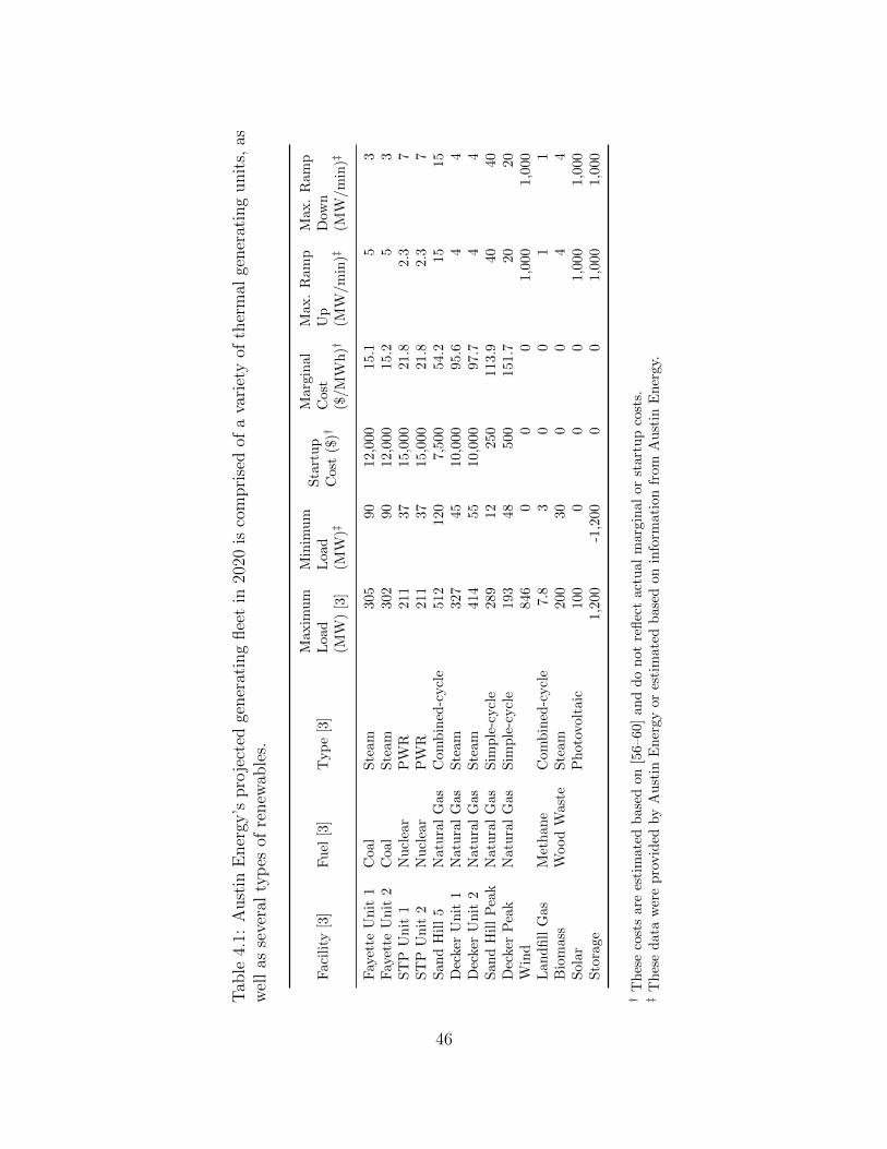
Tab
le4.
1:A
ust
inE
ner
gy’s
pro
ject
edge
ner
atin
gflee
tin
2020
isco
mpri
sed
ofa
vari
ety
ofth
erm
alge
ner
atin
gunit
s,as
wel
las
seve
ral
typ
esof
renew
able
s.
Fac
ilit
y[3
]F
uel
[3]
Typ
e[3
]M
axim
um
Load
(MW
)[3
]
Min
imu
mL
oad
(MW
)‡
Sta
rtu
pC
ost
($)†
Marg
inal
Cost
($/M
Wh
)†
Max.
Ram
pU
p(M
W/m
in)‡
Max.
Ram
pD
own
(MW
/m
in)‡
Fay
ette
Un
it1
Coa
lS
team
305
90
12,0
00
15.1
53
Fay
ette
Un
it2
Coa
lS
team
302
90
12,0
00
15.2
53
ST
PU
nit
1N
ucl
ear
PW
R211
37
15,0
00
21.8
2.3
7S
TP
Un
it2
Nu
clea
rP
WR
211
37
15,0
00
21.8
2.3
7S
and
Hil
l5
Nat
ura
lG
asC
omb
ined
-cycl
e512
120
7,5
00
54.2
15
15
Dec
ker
Un
it1
Nat
ura
lG
asS
team
327
45
10,0
00
95.6
44
Dec
ker
Un
it2
Nat
ura
lG
asS
team
414
55
10,0
00
97.7
44
San
dH
ill
Pea
kN
atu
ral
Gas
Sim
ple
-cycl
e289
12
250
113.9
40
40
Dec
ker
Pea
kN
atu
ral
Gas
Sim
ple
-cycl
e193
48
500
151.7
20
20
Win
d846
00
01,0
00
1,0
00
Lan
dfi
llG
asM
eth
ane
Com
bin
ed-c
ycl
e7.8
30
01
1B
iom
ass
Wood
Was
teS
team
200
30
00
44
Sol
arP
hot
ovol
taic
100
00
01,0
00
1,0
00
Sto
rage
1,2
00
-1,2
00
00
1,0
00
1,0
00
†T
hes
eco
sts
are
esti
mat
edb
ased
on[5
6–60
]an
dd
on
ot
reflec
tact
ual
marg
inal
or
start
up
cost
s.‡
Th
ese
dat
aw
ere
pro
vid
edby
Au
stin
Ener
gyor
esti
mate
db
ase
don
info
rmati
on
from
Au
stin
En
ergy.
46

2020
2008
Nameplate Capacity (MW)
0 1000 2000 3000 4000
Coal Nuclear Natural Gas Gas Turbines Wind Solar PV Biomass
Figure 4.1: Nearly all of Austin Energy’s planned generation growth by 2020 will befrom renewable sources. [3]
plants in the United States. NOx and CO2 emissions (lbs and tons, respectively) and
load levels (MW) for all of Austin Energy’s generators were, with MATLAB’s regres-
sion function polyfit, transformed into linear regressions. A quadratic example of the
data available and a regression from polyfit are shown in figure 4.2. Because CEMS
data for Decker’s gas turbines is not consistent with the physical limits of those fa-
cilities, all gas turbines in the fleet will be approximated to the emissions rates of
Sand Hill unit 1. This approximation might distort emissions price scenario dispatch
since the gas turbines at Decker are 21 years older than those at Sand Hill, but it will
likely have a minimal effect on unit commitment since the gas turbines at Decker are
almost never used. The gas turbines at Sand Hill are assumed to have homogeneous
emissions rates.
As shown in figure 4.1, Austin Energy’s renewable generating fleet will grow
significantly by 2020. Energy storage is likely to have the greatest benefit after this
growth in installed wind capacity, so this future scenario has been modeled. Austin
47

0 50 100 150 200 250 300
050
100
150
200
Plant Load (MW)
CO
2 Em
issi
ons
(ton
s)
CEMS DataLinear Regression (MATLAB)
Figure 4.2: Decker Power Plant unit 1 CO2 emissions are modeled as proportionalto generator load (MW), a reasonable approximation that avoids introducing non-linearities to the model. [61]
48

Table 4.2: Emission rates for all thermal generators are passed to the model to studythe effect of emissions pricing on storage allocation and unit commitment decisions.
Emission Plant Rate (tons/MW) Base Level (tons)
CO2 Decker 1 5.5e-01 9.44CO2 Decker 2 5.5e-01 10.1CO2 Decker GT‡ - -CO2 Fayette 1 9.7e-01 20.5CO2 Fayette 2 9.9e-01 16.4CO2 Sand Hill GT 6.6e-01 -2.51CO2 Sand Hill 5 3.6e-01 13.5
NOx Decker 1† 7.6e-04 -2.9e-02NOx Decker 2† 5.5e-04 -2.5e-02NOx Decker GT‡ - -NOx Fayette 1 4.4e-04 4.7e-02NOx Fayette 2 5.6e-04 -1.9e-02NOx Sand Hill GT 7.4e-05 2.3e-03NOx Sand Hill 5 2.6e-05 9.6e-03
† Most cases were an acceptable linear fit but these emission rates were not.‡ Since Decker gas turbine data were not properly reported in CEMS, these are taken in the modelto be equal to Sand Hill gas turbine reported data
49
Energy has estimated that their peak requirements will increase by 238 MW from
2008 to 2020, assuming their DSM efforts in the intervening years are successful. [3]
Load data provided by Austin Energy for 2008 in 15-minute increments was scaled
by finding the peak of that year and increasing it by 238 MW. Time periods where
demand was less than peak were increased by a fraction of 238 MW based on the
fraction of demand in that period compared to peak 2008 demand. As an example, if
the peak in 2008 was 2000 MW and the time period of interest had, in 2008, a load
of 1500 MW, the adjusted value for 2020 in that period would be 1500/2000 · 238 +
1500 MW.
Using a similar approach to demand scaling, wind and solar availability were
scaled based on anticipated increases in installed capacity between 2008 and 2020.
Existing wind generation data provided by Austin Energy from their Sweetwater,
Hackberry, Whirlwind and King Mountain facilities was aggregated and scaled up to
the anticipated 846 MW of peak generation available in 2020. Since wind generation
rarely reaches its peak capacity, 2008 wind availability was scaled according to its 2008
percentage of peak — if in some time period in 2008 wind availability was 137 MW,
or 50% of peak, then in 2020, that value was scaled to 50% of 846 MW, or 423 MW.
It is currently unknown whether, as more wind generation is installed at existing and
new sites based on CREZ locations, variability will scale directly as assumed here,
or be reduced due to geographic wind turbine diversification or other factors. Unlike
wind, where existing generation was scaled to fit future capacity, insufficient solar
generation is currently in Austin Energy’s fleet for similar assumptions to be made.
Instead, data from the National Solar Radiation Database (NSRDB) were used to
estimate future solar photovoltaic generation. [62] New Braunfels, TX (site 722416)
was the closest NSRDB site to Austin Energy’s planned solar photovoltaic facility
in Webberville, TX. Hourly total solar insolation data from 2004 were converted to
50

power output using planned peak capacity of 100 MW and an assumed panel efficiency
of 19%. Since data with a higher sampling rate were not available, it was assumed
that solar radiation remained constant throughout each hour period in the model. It
should be noted that since stochastic programming is avoided in these models, it is
assumed that all wind and solar generation provided as inputs to the model for all
time steps will be dispatched at those levels.
In later model variations, storage can be selected from a set of available storage
types. As discussed in section 4.1, because the size of the time steps in these models,
storage will either be used for arbitrage or not selected; hence, the storage types
provided to the model are those that are both available in Texas and suitable for
daily storage. Because of geographic restrictions, pumped hydroelectric storage is
not included. The parameters shown in table 4.3 detail the operating constraints
on a typical energy storage unit — charge and discharge rates (MW), charge and
discharge ramp rates (MW/min), fixed ($/MW-year) and variable marginal costs
($/MWh), round-trip efficiency, and total capacity (MWh). Each storage type shown
in table 4.3 provides details for a typical single unit. The model is able to select
a nearly unlimited number of units and a combination of different storage types to
reach optimality. It should be noted that the number of PHEVs are restricted to
12,000, which represents roughly 3% of the vehicles in the Austin Energy service area
and is an approximation of an upper limit for PHEV market penetration in the region
after slightly less than one decade of widespread commercial availability. PHEVs are
treated as zero cost storage for the utility, which assumes that customers will receive
no benefits from the utility for the use of their battery. While this arrangement is
unlikely, so many compensation or incentive structures are possible that it is outside
the scope of this study to explore which might be most appropriate or to assume that
one particular approach will achieve market acceptance. Also, PHEVs are assumed
51

Tab
le4.
3:F
orth
epurp
oses
ofth
isst
udy,
asm
all
subse
tof
stor
age
typ
eshas
bee
nse
lect
edbas
edon
thei
rco
stan
dp
erfo
rman
ceat
trib
ute
s.
Typ
eR
oun
d-t
rip
Effi
cien
cy
Typ
ical
Siz
e(M
Wh
)
Maxim
um
Inp
ut
(MW
)
Maxim
um
Ou
tpu
t(M
W)
Ch
arg
eR
am
pR
ate
(MW
/m
in)
Dis
charg
eR
am
pR
ate
(MW
/m
in)
Fix
edM
arg
inal
Cost
s($
/M
W-y
ear)
Vari
ab
leM
arg
inal
Cost
s($
/M
Wh
)
NaS
Bat
tery
[18]
0.88
0.43
0.0
50.0
50.0
50.0
542,2
00
0V
anad
ium
FB
[18]
0.85
100
10
10
0.5
0.5
56,1
00
0P
HE
Vs
[63]
0.9
0.01
160.0
10.0
10.0
05
0.0
05
00
CA
ES
[14]
1.25†
10,0
00270
200
20
270
108,0
00
1.5
†H
eat
isad
ded
,ty
pic
ally
by
bu
rnin
gn
atu
ral
gas,
tora
ise
the
tem
per
atu
reof
the
ou
tflow
stre
am
bef
ore
exp
an
din
git
ina
turb
ine
train
,m
akin
gth
eto
tal
ener
gyex
trac
ted
grea
ter
than
that
store
d.
[14]
52

to be available whenever the utility wants to use their stored electricity and that
their charge level does not vary apart from when the utility dispatches them. This
assumption is not realistic since owners are likely to use their cars throughout the
day and reconnect them to the grid at varying levels of charge. The details of V2G
interactions of PHEVs are, however, outside the scope of this study and neglecting
them minimizes computational requirements for modeling PHEVs as a possible energy
storage option.
4.3 Model Structure
GAMS, used to implement the unit commitment models presented here, im-
poses a specific structure on those models. In GAMS, governing sets, or variable and
parameter indices, are declared first. Parameters — variables with fixed values that
typically describe components in the modeled system — are declared and assigned
values directly in the code or, as in this model, read from a GDX file, which enables
the use of Excel for data entry and promotes code brevity. Finally, scalars and vari-
ables are declared and described. All of these components are then combined into
equations that follow a form nearly identical to that presented in section 4.4. This
approach creates a structure that can be conveniently represented, as has been done
in tables 4.4 through 4.8.
These models were originally structured such that results for cases with and
without storage were captured with one GAMS file. Since each variable must have a
single index associated with it, structuring the model in this way led to many different
variable names, making the code excessively long and difficult to follow. With added
equations to capture more constraints, the model was transitioned to a structure
where each version had only two indices, one for those parameters and variables that
53

Table 4.4: GAMS models are structured around controlling indices called “sets.”
Index (Set) Description
g All generating units (Table 4.1)t Model time periods in 15-minute increments
Table 4.5: Model parameters define the operating constraints of all generators in table4.1, as well as time-dependent functions.
Parameter Description
mcg Marginal costs for all generators g ($/MW)maxpowerg Generator nameplate (maximum) capacity (MW)minpowerg Minimum generator operating level (MW)rampupg Ramp rate increase limit (MW/min)rampdowng Ramp rate decrease limit (MW/min)startcostg Startup costs for all generators g ($)demandt Demand in each period (MW)windt Aggregated wind availability (deterministic) in each period (MW)†
solart Solar availability (deterministic) in each period (MW)emissionsg Emissions rate based on plant output (tons/MW or lbs/MW)interceptg Base level emissions rate from each generator (tons or pounds)
† Wind availability is aggregated over all Austin Energy’s contracted wind farms
change for every generator g and one for those that vary throughout the modeled time
t. As indicated in table 4.4, in all models presented here, regardless of the length of
the model, only 15-minute time steps are used.
The parameters in table 4.5 are almost entirely identical to the column head-
ings in tables 4.1 and 4.2. Those parameters that vary with t : deterministic demand,
wind and solar availability, are added here. These parameters are known for the full
model period, regardless of its length, and all ‘available’ wind and solar generation
must be dispatched. Thermal generators must respond to compensate for changes
from these and other renewable generators, as they do in Austin Energy’s current
54

Table 4.6: Model variables are combined with parameters to form the objective func-tion and constraint equations.
Variable Description
ong, t Binary indicating plant g turned on in period toffg, t Binary indicating plant g shut off in period t-1sprg, t Spinning reserve quantity provided by plant g in period txg, t Power generated by unit g in period t (MW)yg, t Binary indicating if a unit g is on in period tz Objective function
system. Recall, however, that applying stochastic methods to model these parame-
ters would not significantly improve commitment or dispatch decisions. [22,37]
In addition to the parameters in table 4.5, three scalars are used in the model.
The quantity of spinning reserve that must be held in the model, following the 90 MW
guideline used by Austin Energy, is controlled by resamt. The marginal cost of the
two nuclear generators, South Texas Project units 1 and 2, is adjusted by $7/MWh
using scalar nukecdt so that their marginal prices are below that of the cheapest
generator indicated in 4.1. The modification of the nuclear generators’ marginal
costs is to ensure that they are always fully dispatched and that, if needed, Fayette
Power Project’s generators are dialed back first. Finally, the scalar price captures
the market price of the relevant emissions factor for scenarios that include emissions
pricing.
Binary variables ong, t and offg, t indicate when a plant has started up or shut
down. These variables will be explained further with the equations that govern their
assignment. Variable sprg, t ensures that sufficient spinning reserve, governed by re-
samt, is always allocated. In the model, only Fayette units 1 and 2, South Texas
Project units 1 and 2, Sand Hill unit 5 (combined-cycle) and Decker units 1 and 2
55

are permitted to provide spinning reserve only when they are on, or when their yg, t is
equal to 1. When storage is available, it is also permitted to provide spinning reserve,
though market protocols dictated by ERCOT do not explicitly allow the use of energy
storage for spinning reserves. The dispatch of every plant g for all times t is assigned
to the variable xg, t, where in all periods that x is non-zero, yg, t must be equal to one,
indicating that the plant is on. The variable z captures the value of the objective
function and is passed to the solver for minimization.
For those model cases that include energy storage declared as a thermal gener-
ator, the variable xg, t, where g refers to storage, can only be constrained in ways that
make sense for thermal generators. As a result, this model structure cannot, without
additional equations, fully describe a unit of energy storage. Since the goal of this
work is to reveal what storage types are best suited to energy storage in the grid and
at what price points those storage facilities might be practical, improved modeling
of energy storage is needed. A third model index (set), type, is declared to facilitate
selection of discrete storage types. All the storage units that can be selected, based on
table 4.3, are indexed over this set. As with thermal generators, constraints must be
declared to govern the operation of each of these storage units of type by converting
most of the columns in table 4.3 into parameters in table 4.7.
To capture round trip efficiency, withdrawals (outtype, t) from energy storage are
measured separately from inflows (intype, t). These values are constrained by maximum
withdrawals and inflows in every time period, as well as ramp rate changes in those
values. Additionally, the quantity stored, storedtype, t, at every time step t must be
measured to ensure that total storage capacity for each unit is not exceeded. The
information about storage unit performance characteristics given in table 4.3 describes
one characteristic unit of that storage type and ntype, an integer number of those units,
56

Table 4.7: For the discrete storage scenarios, additional parameters are required toenable constraints on their assignment and operation.
Parameter Description
efftype Round-trip efficiency for all storage units of type typesizetype Maximum capacity of one storage unit (MWh)inlimittype Maximum charge rate (MW)outlimittype Maximum discharge rate (MW)chgtype Maximum rate of change of charge rate (MW/min)dischgtype Maximum rate of change of discharge rate (MW/min)fixcosttype Fixed marginal costs ($/MW-year)varcosttype Variable marginal costs ($/MWh)
Table 4.8: Additional variables must be defined to constrain the selection and oper-ation of energy storage in the discrete storage scenarios.
Variable Description
storedtype, t Energy stored in storage unit type at the end of period tintype, t Input to storage type during period touttype, t Output from storage type during period tstrtype, t Spinning reserve provided by storage type during period tntype Number of units of energy storage type available on the grid
57

might be used in the model. Generally, this value is left to be assigned freely by the
model to select the optimal combination of storage types.
4.4 Governing Equations
The model components — sets, parameters and variables — presented in the
previous section come together to form the governing equations for all of the model
setups tested. Below are the specific objective functions and constraint equations that
provide realistic limits on the operation of thermal power plants and energy storage,
in those models that include discrete energy storage selection.
4.4.1 Objective Functions
All models in this work share a common marginal cost minimization objective
function equation. Equation 4.1 includes marginal costs as well as several other
parameters that are included for control or minimization:
z =∑g,t
mcg · xg,t +∑g,t
startcostg · ong,t +∑g,t
(ong,t + off g,t) (4.1)
Equation 4.1 captures major ongoing costs associated with thermal power
generators — operating, fuel and maintenance costs (first term) and startup costs
(second term). Marginal costs are given by table 4.1 except that nukecdt (not shown)
is subtracted from nuclear generator marginal costs to ensure they are the first thermal
generators dispatched. Because renewable generation assets are assigned artificial
marginal costs to ensure their dispatch, this objective does not strictly dispatch based
on marginal costs. Since generation from these units are provided through forward
contracts with IPPs, the terms of those contracts are not disclosed to the public and
thus marginal costs are unknown and not necessarily linked to the price Austin Energy
pays per MWh of generation. Each summation is over all terms in both sets g and
58
t, or generators and time steps, respectively. The way the objective is structured, it
appears that plant turn-ons are penalized twice, but the third term is strictly a control
for the variables ong,t and offg,t so that the model does not arbitrarily assign values
of 1 to those variables at times when a generator did not turn on or off, respectively.
The importance of this term is explained further with the introduction of equations
4.13 and 4.14. The addition of terms that do not directly affect operating costs would
appear to taint the objective, but including additional variables in the objective is
an effective method for controlling variable assignment and the actual operating cost
can be recalculated once the optimization run is complete.
For models that include discrete storage selection, two additional terms are
appended to the objective given by equation 4.1, shown in equation 4.2:
· · ·∑type,t
(0.25·outtype,t ·varcosttype)+∑type
(ntype ·inlimittype ·fixcosttype ·
cardt35040
)(4.2)
These terms calculate the variable and fixed marginal costs for those storage
types employed in the model. The value 35040 on the second term divides the length
of the model (cardt) by the length of a year to calculate the total fixed marginal costs
for the modeled period.
To capture the effect of potential future emissions pricing or markets, equation
section 4.3 is added to the objective:
· · ·∑g,t
price(emissionsg · xg,t + minimumg · yg,t) (4.3)
These terms calculate the emissions rate for any thermal generator g based
on historical CEMS data, detailed in section 4.2. The price is provided to the model
in $20/ton increments from $10/ton to $90/ton for CO2 and $10/lb increments from
$5/lb to $45/lb. The first term inside the parentheses describes the emissions rate
59

(tons/MW or lbs/MW) and the second term is the base level emissions quantity (tons
or lbs). These quantities are in table 4.2.
4.4.2 Constraint Equations
Each of the following equations serves to constrain operation of the model,
reflecting realistic physical constraints on generator operation. Some previous unit
commitment models neglect certain constraints, such as startup costs and minimum
load levels, but such omissions can significantly affect results. [20] In all unit commit-
ment systems, as in all real electricity generation and distribution systems, demand
must be met at all times. Equation 4.4 strictly requires the model to turn on sufficient
generating units to meet or exceed demand:
∑g
xg,t −∑type
intype,t +∑type
(outtype,t · eff type) ≥ demandt ∀ t (4.4)
The relation between dispatch (xg,t) and demand (demandt) implies that unit
commitment could exceed demand, but because the objective to be minimized in-
cludes the dispatch term, demand will likely never be exceeded. Equation 4.4 is
dependent on the set t, thus, it is applied for all times t in the model formulation,
as indicated by ∀ t. Here, equation 4.4 includes terms with the variables intype,t and
outtype,t, which are only included for those models that have discrete storage selection.
An alternate formulation could include a slack variable q on the left-hand side of the
equation, allowing the model to not meet demand by assigning a positive value to
q. The slack variable would appear in the objective function, multiplied by a large
scalar value, penalizing the failure to meet demand. This approach could realisti-
cally represent the costs or penalties, if known, associated with blackouts or the use
of resource entities. This approach was tested during model development and the
value of penalty is crucial — if it is too small, the model will pay the penalty instead
60

of dispatching any generators and, if it is too large, it will never be used— so this
approach is avoided in the interest of determining unit commitment apart from the
availability of demand as a resource.
For all generating units modeled, there exist minimum and maximum operat-
ing levels, applied to unit commitment variable xg,t with equations 4.5 and 4.6:
xg,t ≥ yg,t ·minpowerg ∀ g, t (4.5)
xg,t + sprg,t
∣∣∣g < 7≤ yg,t ·maxpowerg ∀ g, t (4.6)
These reflect real constraints on the rotating equipment of power plants, which
can only generate electricity at a range of operating levels. Additionally, for those
plants that are permitted to provide spinning reserve, indicated by the restriction on
sprg,t, they must not provide more spinning reserve than is possible while remaining
under nameplate capacity. Both equations apply for all units g during all periods t. To
permit initial commitment at any allowable level between minpowerg and maxpowerg
(or 0), these equations are not applied in the first time step to. Notably, units are
not required to remain off for a specified amount of time through these or other
constraint equations, as the penalty applied to generator startup, included in the
objective function, ensures that repeated unit startup and shutdown will be avoided.
Equations 4.5 and 4.6 also control the assignment of binary yg,t, which indicates
whether a unit g is operating in period t. This variable will be important in the
assignment of binaries ong,t and offg,t in equations 4.13 and 4.14.
Typically, thermal power plants are constrained in their ability to change their
power output level quickly. Additionally, when they turn on, they are not able to
immediately provide generation up to their nameplate capacity. [31] For all time steps
beyond initial commitment period to, equations 4.7 and 4.8 control unit commitment
61

consistent with these limitations:
xg,t−xg,t−1 +sprg,t
∣∣∣g < 7≤ 15 ·minpowerg ·off g,t−rampupg (yg,t−ong,t) ∀g, t (4.7)
xg,t − xg,t−1 ≥ −minpowerg · off g,t − 15 · rampdowng (yg,t−1 − off g.t) ∀ g, t (4.8)
As with equations 4.5 and 4.6, equations 4.7 and 4.8 are not applied until
after to to allow initial commitment and dispatch, after which time any generator g
can be committed to no more than its previous generation level plus its maximum
ramp rate up, rampupg, or less than its previous generation minus its ramp rate
down, rampdowng. Ramp rates are specified in MW per minute, as in table 4.3, so
those values are multiplied by 15 in equations 4.7 and 4.8 to yield ramp rate for the
time step. Each of these equations applies to all generators g during all periods t.
Additionally, spinning reserve from those plants that are permitted to provide it must
not exceed the ramp up capability of that generator, thus it is included in equation
4.7.
For all generators that are permitted to provide spinning reserve, total reserve
available for all times t must be greater than resamt of 90 MW, the amount of reserve
held by Austin Energy:∑g
sprg,t
∣∣∣g < 7
+∑type
(strtype,t · eff type)∣∣∣type 6=3
≥ 90 ∀ t (4.9)
For scenarios with discrete storage selection, equation 4.9 follows the form
shown, including spinning reserve from thermal generators and from available storage
types except PHEVs. Where energy storage is treated similarly to other thermal
generators, the strtype term is eliminated and the first term is expanded to include
generic storage.
Because renewable power sources are modeled without marginal costs (table
4.1), it is likely that regardless of the selected objective, all renewables will be fully
62

dispatched by the model. Because of the contractual arrangements with IPPs to
furnish power from these sources, however, a deterministic approach is applied with
equations 4.10, 4.11 and 4.12, forcing the model to use all available renewable gener-
ation in all periods t :
xg,t
∣∣∣g=10
= windt ∀ t (4.10)
xg,t
∣∣∣g=13
= solart ∀ t (4.11)
xg,t = maxpowerg ∀ g∣∣∣g=11,12
, t (4.12)
Recall that wind and solar resources are calculated based on averages of their
generation profiles for every month in 2008, scaled up to correspond with Austin
Energy’s 2020 generation plans. Seasonally adjusted values are provided for both
generation types.
Equations 4.13 and 4.14 do not strictly describe constraints, but they are used
frequently in constraint equations. Equation 4.13 governs the assignment of variable
ong,t during all time steps beyond to (to avoid penalizing initial commitment), where
ong,t is a binary equal to 1 when a unit g is turned on in time t. Similarly, Equation
4.14 controls binary offg,t, which is equal to 1 when a unit g is turned off in time t-1 :
ong,t ≥ yg,t − yg,t−1 ∀ g, t (4.13)
off g,t ≥ yg,t−1 − yg,t ∀ g, t (4.14)
These equations are important in deactivating constraints that should not be
applied to a generator in a period t when it turns on or off. It might seem immediately
apparent that these relationships should be equalities, but if that were the case, during
time periods when a unit turns on, equation 4.14 would try to assign a value of -1
to the binary, with similar results from equation 4.13 when a unit turns off. The
63

inequalities allow the binaries to be assigned values of 1 during periods when a unit
is not turning on or off, so the variables ong,t and offg,t are penalized in the objective
function.
4.4.3 Storage-specific Constraints
When storage is treated as simply an added on unit in the model with Austin
Energy’s existing thermal generation, only one additional equation is included in the
model to control the assignment of xg, t for storage:∑t
xstorage, t = 0 (4.15)
In the interest of constraining energy stored or used as little as possible in
any period t, only this constraint is applied. Equation 4.15 requires that whatever is
discharged from storage must be returned by the end of the modeled period, where
round-trip efficiency of the transmission and energy storage system are assumed to
be unity. As it is, this idealization precludes replication of model results with a real
storage portfolio, which motivates later expansion of the modeling of energy storage.
In the case of models where the time period is limited to a single day, equation 4.15
ensures that energy storage is not modeled as a limitless supply of free energy. If the
model were expanded to weeks or months, this constraint would only dictate that
the final and initial state of charge must be the same, allowing variations in state of
charge across multiple-day boundaries if such an operational approach is optimal.
To more realistically model energy storage in the unit commitment framework,
additional equations for the model are developed using the parameters and variables
from tables 4.7 and 4.8. These control the operation of storage to remain within the
constraints presented in table 4.3. It should be noted that these additional equations
do not determine optimal storage location, only portfolio selection. It is possible that
64

the optimal storage portfolio might vary somewhat depending on facility siting, but
answering that question would require significant further model development and is
thus outside the scope of this thesis.
The major constraint equation controlling the use of energy storage defines the
change in the quantity stored in each time step as the difference between the inputs
and outputs in that period:
storedtype, t = storedtype, t−1 + intype, t − outtype, t ∀ type, t (4.16)
Equation 4.16 calculates the energy stored at the end of period t, storedtype, t,
for all periods t and all storage units type. The variable outtype, t measures the amount
discharged from the storage device, where the amount delivered to the grid is outtype, t
multiplied by efftype. This calculation is performed in the thermal generator equation
4.4. Each of the variables represented in this equation capture totals for all n units of
each type of storage selected in the results, which is distinctly different from storage
unit parameters, which must be multiplied by n to determine actual operational
constraints. Upper operational limits are controlled by:
storedtype, t ≤ sizetype · ntype ∀ type, t (4.17)
intype, t ≤ inlimittype · ntype ∀ type, t (4.18)
outtype, t + strtype, t
∣∣∣type 6=3
≤ outlimittype · ntype ∀ type, t (4.19)
Equation 4.17 ensures that total energy stored (MWh) does not exceed the
capacity of the storage unit at any point during the modeled time period. Equations
4.18 and 4.19 control the maximum inflow and discharge for all storage devices selected
by the model at all times t. In these, as in all subsequent equations here, where a
parameter appears in the equation it must be multiplied by n, the number of that
65

storage unit type that have been selected. In equation 4.19, as in all equations where
strtype, t appears, spinning reserve from storage cannot be provided by PHEVs. In
the model, this restriction is applied directly to the variable strtype, t in the equation
declaration.
In addition to limiting inflow and discharge or outflow for all storage types,
the rate of change in these values must also be controlled:
storedtype, t − storedtype, t−1 ≤ 15 · chgtype · ntype ∀ type, t (4.20)
storedtype, t − storedtype, t−1 − strtype, t ≥ −15 · dischgtype · ntype ∀ type, t (4.21)
In a manner nearly identical to equations 4.7 and 4.8 for thermal power plants,
equations 4.20 and 4.21 control ramp rates for energy storage. Equation 4.21 also
limits spinning reserve quantities that can be provided by a given energy storage type
to no more than what it can ramp to in that period, not including ramping capacity
dispatched.
Finally, regardless of ramp rates, a given energy storage type cannot provide
more reserve than is currently stored:
strtype, t
∣∣∣type 6=3
≤ storedtype, t ∀ type, t (4.22)
Equation 4.22 is entirely restricted to energy storage not provided from PHEVs
because, as mentioned previously, they are not permitted to provide reserve since they
cannot necessarily be expected to be plugged in when the utility wants to dispatch
them. Many other constraints to further limit PHEVs ability to provide storage
require predictions or estimates of owner behavior or desires. Will nighttime stored
energy be available during the day or consumed by commuting, will drivers be able to
plug in their vehicles midday, how much will drivers expect to be paid to comply with
66

utility needs for energy storage from their cars, and will drivers be willing to change
their driving and charging habits to earn more from utilities, are all questions that will
require further study before PHEVs can be fully detailed in a unit commitment model.
Further, it is unlikely that PHEVs will fit neatly into a unit commitment framework
since their availability will likely be non-optimal and subject to only limited control
by the utility.
67

Chapter 5
Results
The results presented henceforth step through the evolution of the model as
functionality and accuracy are added. Section 5.1 presents the first set of results,
where the future generation scenario to be examined is separated into averages for
each month in the year. Demand, wind, and solar generation in these results are all
averages of every day in the month. Each month is modeled discretely, shortening
solution times and providing a clear quantitative look at the potential benefits of
energy storage and the trends that might appear in the full-year models. These
results suggest that meaningful outcomes might be revealed in a full-year model,
but these models require significant computational resources, so fewer scenarios are
studied.
For the full-year models, results from scenarios with and without storage are
compared, including scenarios with discrete storage selection from the portfolio in
table 4.3. Current estimated capital costs associated with storage types available to
the model are in table 5.1. These capital costs are included for reference and can
be used to compare with maximum acceptable capital costs backed out from model
results. These results are presented in section 5.2. Capital costs are not captured
in the model; without accurate financing information about existing facilities and
planned expansion, it is difficult to compare them with energy storage. Further, future
prices could decrease due to economies of scale associated with mass production or
improved manufacturing techniques, or increase due to active material or construction
68

Table 5.1: Estimated Capital Costs for Selected Storage Devices [18]
TypePrice($/MWh)
Price($/MW)
Lifetime(years)
NaS Battery 196,000 1,862,000 10Vanadium FB 236,000 2,691,000 20PHEVs 0 0 10CAES 21,830 750,000 25
material costs, thus capital costs are also excluded on the basis of unknown future
storage prices.
In addition to presenting models with and without storage, emissions prices
and how they affect the value proposition for energy storage are explored as well.
Though CO2 emissions are not regulated and NOx markets are not currently present
in Texas, studying the pricing of these emissions parameters is relevant because of the
possibility of future legislation. Since this work examines generation cases in 2020,
it is possible that in these future scenarios, regulations for large emitters of these
pollutants will be in place. A range of prices for each pollutant are tested to examine
how energy storage can manage cost increases associated with changes in dispatch
decisions. All the scenarios studied for this work are summarized in table 5.2.
5.1 Monthly Averaged Demand, Wind and Solar Generation
For these results, each month of demand, wind and solar data were scaled to
match our 2020 scenario of interest, and then all the days each month were averaged
to make a scenario day for study. As a result, these cases can only represent an
average of availability of renewable resources and demand requirements, excluding
cases with the worst renewables availability or highest demand peaks.
69

Table 5.2: Summary of All Scenarios/Cases Presented
Scenario/Case Description
Month-by-Month,24-Hour
Model runs for each month with separate runs for caseswithout storage and with generic, unconstrained storage,all using 2020 scenario conditions for load, wind and solargeneration, and generating fleet capabilities
2008 without Storage A single model execution for a full year using load, windand generating fleet information to validate model dis-patch accuracy against Austin Energy data
2020 without Storage A full-year model using estimated 2020 scenario condi-tions with only thermal generators available for dispatch
2020 with Storage A full year using the estimated 2020 scenario conditionswith generic energy storage available, unconstrained byround-trip efficiency or marginal costs
2020 with DiscreteStorage
A full-year model using 2020 scenario conditions plus en-ergy storage availability based on constraints in table 4.7and integer caps on storage availability in table 5.4
2020 with LimitedDiscrete Storage
A full-year model similar to ‘2020 with Discrete Storage,’but with lower caps on storage availability, shown in table5.5
2020 Storage plusCO2 Prices
Similar to ‘2020 with Storage,’ except with CO2 pricesincluded in the objective function
2020 Storage plusNOx Prices
Similar to ‘2020 with Storage,’ except with NOx pricesincluded in the objective function
70

Time Step [h]
Load
[MW
]
0 2 4 6 8 10 12 14 16 18 20 22
010
0020
0030
00
BiomassLandfill GasSolarWindSand Hill PeakDecker Unit 2
Decker Unit 1Sand HillFayette Unit 2Fayette Unit 1STP Unit 2STP Unit 1
Figure 5.1: Typical dispatch for a July 2020 day requires dialing back or shuttingdown inexpensive units at night and the use of older, dirtier generators to meet peakdemand.
71

Each of these models were run in GAMS, which includes a variety of options
that affect the way the program and solver run. In the case of these monthly average
results, these options were not needed because of the small number of variables in
each model. These were run with the optimality criterion, the value that determines
model termination, set at the default value of 0.1%. Each model took between a few
seconds and a few minutes to complete when running locally in 64-bit Windows 7 on
the MacBook Pro detailed in section 4.1. Figure 5.1 shows a typical 24-hour dispatch
case for July 2020 without storage. To be strictly rigorous, dispatch decisions should
be plotted as a series of bars, one for each 15 minute interval. The model does not
make continuous dispatch decisions, nor is the time interval small enough for the
results to approximate continuous dispatch, but the smoothing between 15 minute
intervals is a reasonable approximation of the dispatch that could be expected if the
time intervals were shortened considerably. Additionally, displaying the results in
this way is easier to follow. It should be noted that while it is assumed here that
dispatch decisions made for each 15 minute increment transition smoothly to the
next interval, in our calculations of costs and storage allocation, it is assumed that
dispatch is constant throughout the interval.
During the hottest months in Texas, May through September, load varies
dramatically between the lowest and highest demand intervals. The high peak is
a consequence of high cooling loads from the hottest afternoon hours coupled with
significant late afternoon activity as people arrive home. At the same time, wind
generation is reduced and solar generation is beginning to taper during these hours,
requiring that Decker generators 1 and 2 turn on. These generators have high NOx
emissions and high heat rates. In Austin Energy’s current operational structure, they
avoid the use of Decker even during peak hours through a 300MW summer power
purchasing agreement (PPA), likely with a cleaner facility. The costs associated with
72

this approach are unknown and it is unknown whether Austin Energy will continue
to engage in forward contracts for summer peak generation, so the model does not
include this or a similar contract.
Conversely, during the evening hours, many generators must be dialed back or
shut down to accommodate large quantities of available renewable energy. Further,
peaking gas turbines were activated to smooth the shutdown and startup of the
Sand Hill combined cycle generator. Further, the second generator at Fayette had to
be dialed back and the first generator briefly curtailed to accommodate renewables
and the shutdown of Sand Hill 5. In reality, it is likely that some wind would be
curtailed to avoid shutting down the combined cycle generator at Sand Hill because
that generator has minimum on and off times of over 24 hours. Because these data
on minimum operating times were not available when these models were run, these
requirements are violated for the combined cycle generator at Sand Hill but could be
included in future work.
With the availability of energy storage, as in figure 5.2, dispatch changes dra-
matically. Though as stated previously, the dispatch of Decker 1 and 2 is typically
avoided with a PPA, with energy storage, neither a PPA nor the dispatch of decker
is required because renewables available at night that would normally require dialing
back inexpensive generators can be shifted to the day, maintaining a relatively con-
stant level of generation throughout the day. The lightly shaded purple area between
the red and black lines shows where energy is stored at night and then returned to
the grid during peak hours. The cheapest generators, South Texas Project 1 and 2
(nuclear), Fayette 1 and 2 (coal) and Sand Hill 5 (natural gas combined cycle) are
operated at or near full capacity all day, while more expensive generators are entirely
avoided. Because of the availability of energy storage, dispatch requires only these
73

Time Step [h]
Load
[MW
]
0 2 4 6 8 10 12 14 16 18 20 22
010
0020
0030
00
StorageBiomassLandfill GasSolarWind
Sand HillFayette Unit 2Fayette Unit 1STP Unit 2STP Unit 1
Without StorageWith Storage
Figure 5.2: Dispatch with available storage in a July 2020 day meets peak demand us-ing wind energy available at night, avoiding the use of expensive and dirty generatorsand peaking units.
74

generators and renewable sources to meet demand throughout the day, even as de-
mand varies significantly. The drop in dispatch of Sand Hill 5 from maximum to
minimum load for a few hours in the evening is a consequence of needing to discharge
all stored energy, as required by equation 4.15. These models do not include non-linear
plant efficiencies that would likely discourage operating any generator at minimum
load except to avoid startup penalties. If these non-linearities were captured, Sand
Hill would probably be dialed back slightly throughout the dispatch period instead.
Cooler days in winter and spring months are characterized by demand that
is much flatter throughout the day, as in figure 5.3. The largest change between
the lowest and highest demand intervals during these months might only be a few
hundred megawatts. These months also have the highest wind availability, resulting in
significant curtailment of generation from baseload units throughout the day. Again,
it is likely that some wind generation would be curtailed to ensure the nuclear facility
could continue to operate at maximum output. Because demand is low and flat
throughout the day, most demand can be met with baseload generators Fayette and
South Texas Project, but for a few hours each day, peaking generators or a Decker
unit might be used to meet demand. This dispatch does not best utilize inexpensive
thermal generation, since baseload generators must be curtailed during nighttime
hours to accommodate renewable capacity.
Since winter and spring demand varies little between maximum and minimum
periods, figure 5.4 shows it can be served almost entirely by baseload generation
and available renewables. Even with the minimal variation in load, some peaking
generation is still required because renewables in Austin Energy’s portfolio are not
well-phased for peak demand. With energy storage, this generation can be avoided by
storing some wind generation during the nighttime hours and dispatching it during
75

Time Step [h]
Load
[MW
]
0 2 4 6 8 10 12 14 16 18 20 22
010
0020
0030
00
BiomassLandfill GasSolarWindSand Hill Peak
Decker Unit 1Fayette Unit 2Fayette Unit 1STP Unit 2STP Unit 1
Figure 5.3: In a November 2020 day, as with most winter and spring months in Texas,demand can be served almost entirely by baseload generation and renewables becausevariations during the day are limited.
76

Time Step [h]
Load
[MW
]
0 2 4 6 8 10 12 14 16 18 20 22
010
0020
0030
00
StorageBiomassLandfill GasSolarWind
Fayette Unit 2Fayette Unit 1STP Unit 2STP Unit 1
Without StorageWith Storage
Figure 5.4: As with the November 2020 scenario without storage, demand varieslittle throughout the day and is served by inexpensive generators, yielding minimalopportunity for benefit from energy storage availability.
77

the daytime peak. Further, the limited variation in demand means that little storage
is required to accommodate peak load. In some cooler months, allocation of energy
storage might be characterized by a series of charge and discharge intervals if there is
not a singular peak in demand. In all the cases shown in figures 5.1 through 5.4 and
all other observed cases, regardless of the number of charge and discharge periods or
the magnitude of the peak during the day, the optimal level of storage is whatever is
required to maintain flat or nearly flat total dispatch throughout the day, enabling
the use of inexpensive generators throughout the day and the avoidance of expensive
facilities like Decker and simple cycle gas turbines.
Similar to figure 5.3, figure 5.6 shows dispatch during a cool fall month when
load is nearly flat throughout the day. Again here, some generation from an expensive
and inefficient facility is required during the brief peak period. In each of these cases
where the coal facility is partially dispatched on at least one generator, the mismatch
in the dispatch of the two units is likely a consequence of not modeling the non-linear
efficiencies of these generators. If these non-linearities were included, both units would
likely be dispatched equally. Regardless, the predicted cost of dispatch, assuming the
average linear heat rates used as proxies for non-linear data are consistent with real
plant efficiency, should still be predicted correctly by this model.
As in a few other winter and spring months, in figure 5.6 Fayette 1 is dispatched
with significant seemingly random variations throughout the day. This behavior is
also likely a consequence of not including non-linear heat rates for thermal generating
facilities. If those were included, then it is likely the dispatch of Fayette 1 would
be smoothed somewhat, operating at a sustained lower level that is preferred to the
frequent ramping between maximum load and some lower level. Since storage is
available, smoother dispatch of this generator is definitely feasible, as in figure 5.4.
78
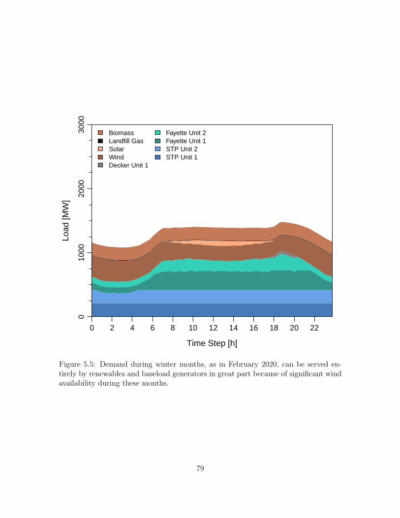
Time Step [h]
Load
[MW
]
0 2 4 6 8 10 12 14 16 18 20 22
010
0020
0030
00
BiomassLandfill GasSolarWindDecker Unit 1
Fayette Unit 2Fayette Unit 1STP Unit 2STP Unit 1
Figure 5.5: Demand during winter months, as in February 2020, can be served en-tirely by renewables and baseload generators in great part because of significant windavailability during these months.
79

Time Step [h]
Load
[MW
]
0 2 4 6 8 10 12 14 16 18 20 22
010
0020
0030
00
StorageBiomassLandfill GasSolarWind
Fayette Unit 2Fayette Unit 1STP Unit 2STP Unit 1
Without StorageWith Storage
Figure 5.6: In the modeled February 2020 day, frequent ramping of some generatorsappears, as in several other dispatch results with storage, likely a consequence of theuse of linear marginal costs for these results.
80

This dispatch being returned as optimal by the solver is possibly the consequence of
there existing several nearly identical minima in the problem’s solution space. As
mentioned before, it is also likely that with non-linear heat rates in the model, the
dispatch of the two coal generators would be the same instead of Fayette 2 operating
at minimum load throughout the day.
Looking broadly at the effect of energy storage on dispatch throughout the
year, as in figure 5.7, there are several important trends to note in the operation of
Austin Energy’s generating fleet. The optimal allocation of energy storage appears to
scale roughly with the cost of generation for the marginal (price setting) generator.
As the cost of generation increases, so does the presence of energy storage. In each
of these cases, total stored energy appears to capture only renewables. While this
observation is not strictly correct since, as seen in figure 5.2, in some nighttime
intervals, natural gas generation is also stored, during most intervals in most months
modeled, all stored energy is from renewable sources. Even without examining the
dispatch curves from every month to validate this conclusion, considering that most
renewables are from wind, which is most available at night in Texas, in months when
less than half of total renewable generation is stored and more than half of total
renewables are available at night, it is likely that all or nearly all stored energy is
from renewable sources. Further, overall utilization of the most inexpensive and
efficient plants in the fleet is enabled with the availability of energy storage. This
trend is most obvious in intermediate months like April, May and October, where
the cases with storage show a marked increase in coal dispatch and a corresponding
reduction in the use of natural gas facilities. In summer months where natural gas
dispatch appears unchanged, there is an increase in the use of the cheaper and cleaner
combined cycle unit at Sand Hill and a reduction or elimination of dispatch of Decker
1 and 2, as seen in figure 5.2. If non-linear heat rates and emissions rates were
81

December
November
October
September
August
July
June
May
April
March
February
(With Storage)
January
24 Hour Total Electricity Dispatched (MWh)
0 10000 20000 30000 40000 50000
Nuclear Coal Natural Gas Gas Turbines Renewables Storage
Figure 5.7: In most months, the availability of energy storage maximizes the dispatchof inexpensive generators by shaping wind output.
82

included in the model, improvements in dispatch with energy storage would likely
increase. Non-linear parameters would signal in the model what operating point is
preferred based on the objective function and it has already been shown that energy
storage enables superior dispatch of generating assets.
Comparing the costs of dispatch and allocation of storage, shown in figure 5.8,
between cases with and without storage for each month, it appears that allocation
of energy storage roughly scales with the benefit it provides to dispatch, just as it
scales with the availability of renewables, as seen in figure 5.7. WIth the increased
dispatch of cheaper units shown in figure 5.7, significant cost savings are realized in
most months. In particular, by dispatching the combined cycle unit at Sand Hill and
shaping renewables to correspond with demand, the use of Decker 1 and 2 can be
avoided, providing significant cost reduction. Looking closely at February and March
in figure 5.7, dispatch of less than 100 MW of natural gas generation is replaced by
stored energy between the cases with and without storage but more than 1000 MW
of energy is stored. This small change is likely a consequence of significant renewables
that are not timed appropriately to meet demand and inexpensive baseload generators
that are sufficient to meet almost all remaining demand. Redistributing renewable
generation to peak hours and avoiding the dispatch of peaking generators or one of the
units at Decker for a brief period cannot provide significant cost reductions but might
require a lot of storage. If seasonal storage were available, enabling the operation of
South Texas Project and Fayette generators at full capacity and capturing any excess
renewables could provide significant benefit if returned to the grid during the summer
months, when renewables are less readily available. In examining the results of energy
storage allocation in the full-year models, it turns out this approach is the optimal
allocation of energy storage if it is not quantity limited.
83
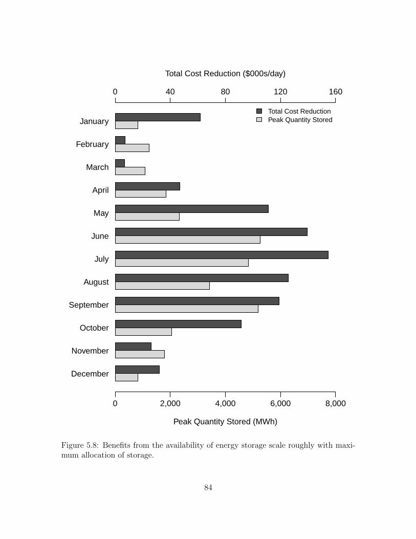
December
November
October
September
August
July
June
May
April
March
February
January
Peak Quantity Stored (MWh)
0 40 80 120 160
0 2,000 4,000 6,000 8,000
Total Cost Reduction ($000s/day)
Total Cost ReductionPeak Quantity Stored
Figure 5.8: Benefits from the availability of energy storage scale roughly with maxi-mum allocation of storage.
84

5.2 Year-long Results with Storage
Following on from the results in section 5.1 comparing average days in each
month using the 2020 scenario conditions detailed earlier, a series of year long models
with energy storage are examined to determine if the effects of storage — leveling
of load and increasing dispatch of cheap and efficient thermal generating units while
avoiding more expensive peaking generators — persist with a full year of dispatch.
These year-long models will facilitate study of the hypothesis based on the results in
figures 5.7 and 5.8 that seasonal storage might be able to provide additional dispatch
improvements and cost reductions over daily arbitrage. The impact of including
round-trip efficiencies, marginal costs and other storage constraints from table 4.3 on
energy storage allocation is examined. The types of storage selected by the model,
and the effect of varying integer limits on discrete energy storage allocation are also
studied with a set of discrete storage selection models.
Because of the size of these models, options available in GAMS and CPLEX
have been leveraged to decrease the solution time and preserve HPC resources for
other users. These options are detailed in appendix A, table A.1. Rolling planning is
also employed, using a technique similar to that suggested by [22] and [43] . As shown
in figure 5.9, each case uses a five-iteration rolling planning horizon. This approach
shortens solution time by solving only a small portion of the problem with the integer
constraints intact (green), relaxing the integer constraints in the portion of the model
not yet studied as a MIP (red), transforming that portion into an easier-to-solve LP.
The portion of the model already studied as a MIP has its integer variables fixed to
the values determined by the MIP solution (blue). This approach means in any given
solution case, the time spent solving the MIP is greatly reduced and the size of the
problem that is not at least partially characterized shrinks with each iteration.
85

5
4
3
2
Iteration 1
Time Step
0 5856 11712 17568 23424 29280 35136
Fixed MIP Relaxed (LP)
Figure 5.9: With a rolling planning solution method, the portion of the model solvedas a full mixed-integer program is limited to a section of the full study length toshorten solution times.
Figure 5.10 confirms the conclusions from figures 5.7 and 5.8 on the effect of
energy storage on economic dispatch decisions. The availability of energy storage in
year-long simulations enable dispatch of the cheapest and most efficient generators
in the fleet, coal and nuclear power facilities. Dispatch of these cheaper but less
flexible generators replaces the use of more expensive and dirty generators during
on-peak hours, particularly Decker 1 and 2 and simple-cycle gas turbines. In addi-
tion to superior utilization of thermal generation, energy storage enables the use of
renewable energy sources during peak hours instead of only the hours when they are
most available. These effects combine to reduce the cost of dispatch by $75 million,
$94 million and $40 million each year for the generic storage, discrete storage and
allocation limited discrete storage models, respectively.
In the comparison in figure 5.7 and in figures 5.12 and 5.13 below, the discrete
energy storage scenarios appears to serve less demand, which is because some of the
86

Limited Discrete
Discrete
Storage
No Storage
Energy Dispatched (MWh)
0.0e+00 3.0e+06 6.0e+06 9.0e+06 1.2e+07 1.5e+07
Nuclear Coal Natural Gas Gas Turbines Renewables
Figure 5.10: As in earlier results, the availability of energy storage improves dispatchof inexpensive generators by shaping renewables availability.
87

traditional thermal generation has been replaced by stored energy returned to the
grid from the CAES facility. The CAES facility modeled here uses natural gas as
a secondary input to the outlet turbines, where the combustion of that natural gas
to preheat the air expanding out of the storage cavern increases the output energy
such that efficiency of the plant appears, on an electricity in versus electricity out
comparison, to be greater than one. This additional electricity from the combustion
of natural gas is the energy displacing other, more expensive facilities.
Each of the figures 5.11, 5.12 and 5.13 show load duration curves adjacent
to histograms that show the total hours of operation for each plotted range of load
levels. Load duration plots show each time step of load, 15 minutes in the case of
these results, sorted from highest load to lowest. The histograms paired with each
figure simply show the number of hours load is served in 50 MW increments in the
total load range. Bars to the right of the histogram show the mean and standard
deviation of the two scenarios to further emphasize the effects of storage. Together,
these figures provide a sense of the way load is distributed throughout the year —
either concentrated tightly around a few hundred megawatts that could be served
by a relatively inflexible fleet of generators optimized for these load levels or ranging
many hundreds of megawatts, requiring a wide range of flexible generating units to
respond to varying levels of demand. Each figure compares a single case for storage
with the baseline without storage case.
Figure 5.11 illustrates the effect of energy storage availability. In this case,
the quantity of storage available was not restricted. If storage is assigned without
regard to cost or efficiency constraints, while it does not affect the average load
level, it reduces the standard deviation of load from 383 MW to 202 MW. If storage
efficiency were included and if it were not for energy additions from natural gas in
88

Hours in a Year
Load
(M
W)
0 1500 3000 4500 6000 7500 9000
010
0020
0030
00
No StorageStorage
0 2000 4000
Load Histogram (h)
plot
int
MeanStandard Deviation
Figure 5.11: Energy storage flattens demand significantly throughout the year, and asshown in the histogram in the right panel, storage thus reduces the number of hours ofpeak generation and the magnitude of peak requirements while also increasing demandduring the lowest few hours of the year. Average load and standard deviation for eachof these cases are summarized in table 5.3.
89

Hours in a Year
Load
(M
W)
0 1500 3000 4500 6000 7500 9000
010
0020
0030
00No StorageDiscrete Storage
0 2000 4000
Load Histogram (h)
plot
int
MeanStandard Deviation
Figure 5.12: With the presence of CAES, the discrete scenario results show not onlya concentration of load levels to be served, as in figure 5.11, but also a small overallreduction in load.
expansion turbines at CAES facilities, load average would increase. Concentrating
load requirements into a narrow operating range allows sustained operation of the
cheapest and most efficient plants while simultaneously maximizing the usefulness of
renewable power generation, as suggested by figure 5.10. This flattening of demand
throughout the year is especially notable at the extremes, where maximum load is
reduced by 291 MW and minimum load increased by 241 MW.
The discrete energy storage case includes the impacts of energy storage and
captured the primary constraints that describe the operation of the selected energy
storage types, yet it showed a similar result to the generic storage case. The presence
90

Hours in a Year
Load
(M
W)
0 1500 3000 4500 6000 7500 9000
010
0020
0030
00No StorageLimited Discrete Storage
0 2000 4000
Load Histogram (h)
plot
int
MeanStandard Deviation
Figure 5.13: With limited storage available, minimal reshaping of demand occurs,using storage to shift only the most expensive hours of the year, maximizing thebenefit of what storage is available.
of energy storage here yields the same narrowing of operating load requirements, but
load is characterized by a lower average, since, as mentioned before, some additional
generation is provided by natural gas combustion during the release of compressed
air from the CAES storage cavern. This comparison also shows increases in minimum
load and concomitant decreases in maximum load compared to the generic storage
scenario. As mentioned before, the use of CAES that returns more electricity to the
grid than is stored depresses both the minimum and maximum values, yielding a
minimum load increase of only 46 MW and a peak decrease of 708 MW.
Since both the generic and discrete storage scenarios allocated significant quan-
91

tities of storage, the integer limits built into the discrete storage model were used to
test the effect of a more limited portfolio of storage, given in table 5.5. This portfolio
was selected based on current high storage capital costs that might encourage utili-
ties to be initially conservative with energy storage deployment. Given the marginal
benefit of additional storage, this portfolio is not conclusively optimal. With minimal
storage available, the distribution of load throughout the year shown in figure 5.13
is not as concentrated as it is for the unlimited1 storage scenarios. While storage
availability is limited, it is still sufficient to address the highest cost hours of the year.
Storage redistributes generation from lower cost periods to reduce dispatch require-
ments during peak hours. The total cost of this shifted generation, when including
storage marginal costs, is significantly lower than that of peaking generators. With
current capital costs, this result indicates that energy storage should be sized to ad-
dress these highest cost hours first. If storage capital costs decrease in the future,
further storage could be justified.
Regardless of the nature of the storage available, the magnitude of peak de-
mand and the number of hours of high demand are reduced while simultaneously
increasing load during the hours of lowest demand, flattening overall demand through-
out the year. With less storage available, as in the limited discrete storage case, this
effect is less pronounced, though still present. This outcome is consistent with our
month-by-month average results, where load was more consistent throughout the day
with storage than without, regardless of the month of interest. Standard deviation
quantifies this flattening of demand and is summarized for all scenarios in table 5.3.
Month-by-month energy storage in the discrete and generic scenarios in figure
1The model case with discrete energy storage is not strictly ‘unlimited,’ as there are integer limitson the total storage permitted for each type, but these limits are quite high. The significance ofthese limits is discussed at the end of section 5.2.
92

Tab
le5.
3:C
ompar
ing
the
effec
tsof
stor
age
avai
labilit
yre
veal
sth
atev
enlim
ited
stor
age
can
man
age
the
hig
hes
tco
sthou
rsof
the
year
,th
ough
larg
equan
titi
esof
seas
onal
stor
age
has
dra
mat
iceff
ects
ondis
pat
chth
rough
out
the
year
.
Sce
nar
ioA
vera
geL
oad
(MW
)Sta
ndar
dD
evia
tion
(MW
)∆
Max
imum
Loa
d(M
W)
∆M
inim
um
Loa
d(M
W)
Alloca
ted
Sto
rage
(MW
h)
Wit
hou
tSto
rage
1,59
638
2Sto
rage
1,59
620
2–2
9124
12,
218,
745
Dis
cret
eSto
rage
1,53
018
1–7
0846
2,35
4,32
1L
imit
edD
iscr
ete
Sto
rage
1,57
830
8–1
082
13,1
50
93

−4000
0
4000
8000
seq(1, 12)
Net
Qua
ntity
Sto
red
per
Mon
th (
MW
h)
Month−by−Month CasesLimited Discrete Storage
J F M A M J J A S O N D
−270000
−135000
0
135000
270000
Net
Qua
ntity
Sto
red
per
Mon
th (
MW
h)
Month−by−Month CasesGeneric StorageDiscrete StorageLimited Discrete Storage
J F M A M J J A S O N D
Figure 5.14: While there is no clear bias towards storage in one period or anotherwhen quantities or model length are limiting factors, when energy storage quantitiesare unlimited, storage is concentrated primarily in the winter and spring months,when stored energy is the cheapest. It is likely that the difference between genericand discrete storage behavior in the final months of the year is a consequence oflimiting constraints in the discrete storage scenario.
94

5.14 show that allocations are similar in all but the final months of the year, which
is a function of constraints present in the discrete storage scenario that ensure only
energy stored is available for withdrawal, whereas the generic storage case is only
required to return to the original state of charge by the end of the year. This means
that in the generic storage scenario, the storage facility can offer “endless” stored
power, so long as that electricity is returned by the end of the year, which is why that
case has such a large spike at the end of the year.
Looking closely at storage allocations in figure 5.14, it is evident that the
dramatic load leveling that appears in the load duration curves of figures 5.11 and
5.12 is achieved through extensive seasonal energy storage. From January through
May, storage is filled and then throughout the summer, June through September,
storage is fully depleted. Peak storage allocations are not dictated by increasing
peak demand levels, as given by the results in section 5.1, but are, as predicted from
those results, seasonal in nature. Seasonal storage, as allocated by the unlimited
storage cases, stores the cheapest power available in the year — inexpensive baseload
generation and plentiful wind power during the cool fall, winter and spring months
when demand is relatively flat — and returns that power to the grid during the highest
price peak demand periods the hot summer months. This storage approach yields cost
savings of almost $100 million every year, at least four times more than the savings
predicted by the daily price arbitrage use of storage suggested by the results in figure
5.8. Totaling the energy storage allocated month after month in the unlimited storage
scenarios, figure 5.14 reveals that the storage required to achieve this dramatic load
leveling and dispatch improvement is quite sizable, as shown in table 5.3, and while
these operational benefits are significant, the cost of such quantities of energy storage
is likely prohibitive.
95

Table 5.4: If possible, large quantities of energy storage will be allocated by themodel, even when operating costs are included.
NaS Battery Vanadium FB PHEVs CAES
Integer Limit 1,000,000 1,000,000 12,000 1,000,000Optimal Portfolio 999,987 999,987 12,000 999,986MWh Available 429,994 9.9e+07 139.2 9.9e+09
Comparing the generation allocated by the discrete storage model, in table 5.4,
to the quantity actually stored, in table 5.3, it appears that the model has allocated
significantly more storage than needed — nearly 1.0e+10 MWh are available but only
2.2e+06 MWh are stored at the peak in May (from figure 5.14). This appears to be
a consequence of incomplete convergence of the discrete storage scenario, caused by
binding resource constraints, as indicated in table 3.1. Based on the solution path
from the solver, it is evident that the integer values for energy storage were initially
set to their limits and progressively reduced as the solution converged. Since the
marginal cost penalties in the objective did not quickly modulate the assignment of
energy storage, all quantities are higher than necessary. Due to the considerable size
of the solution space for the discrete storage scenario, it might be difficult to reach a
converged solution with existing computing resources. It is likely that the quantity
of storage used, given in table 5.3 represents a more realistic measure of the required
portfolio size.
Based on the results from the year long scenarios with storage, it appears that
seasonal storage is favored. Unfortunately, if left unconstrained, the optimal quan-
tity of seasonal storage is prohibitively expensive, as shown in table 5.6. If storage
allocation is limited, the potential savings associated with storage are comparable to
capital costs for those facilities, given that only the most expensive hours of dispatch
96

Table 5.5: With low limits set for all available energy storage types, the optimaloutcome still appears to be the maximum allowable storage.
NaS Battery Vanadium FB PHEVs CAES
Integer Limit 5,000 10 0 1Optimal Portfolio 5,000 10 0 1MWh Available 2,150 1,000 0 10,000
in the year are addressed. Notably, nearly 75% of the $876 million system cost in the
limited scenario comes from electrochemical energy storage. As already discussed,
the use of storage for arbitrage to address only the highest cost hours of the year
provides the greatest marginal cost benefit. The marginal benefit of additional stor-
age is extremely limited, as evidenced by the unlimited storage scenarios that have
many orders of magnitude more storage capacity, and hence, much higher capital and
marginal costs, but only two to three times greater yearly system operational cost
savings. Payback times for these scenarios do not compare favorably either. The
portfolio in the limited storage case requires around 25 years, on the order of the life-
time of a CAES facility, while the larger storage scenarios require hundreds of years
or more, well beyond the expected lifetimes of the equipment purchased.
Appropriate capital cost targets for energy storage are difficult to determine
directly from these results, as they were not included in the optimization. If inte-
ger limited storage cases were run with progressively increasing portfolio sizes, the
marginal benefit of energy storage could be determined. This could be achieved more
efficiently, however, by directly capturing capital costs. Without these data, cost
trends can still be drawn from existing results. In the limited storage allocation sce-
nario, batteries made up about 75% of the capital cost but provided less than 25% of
total capacity, suggesting that costs for batteries will need to decline significantly be-
97

Table 5.6: Comparing capital costs to annual savings for each of the storage scenariossuggests the limited storage portfolio provides the best economic basis for implemen-tation.
ScenarioAllocatedStorage (MWh)
Capital Cost($ million)†
Cost Reduction($ million/year)
Storage 2.2e+06 52,800‡ 75Discrete Storage 1.0e+10 240,000,000 94Limited Storage 13,150 876 40
† Costs estimated based on $/MWh in table 5.1, not combined cost with $/MW‡ Capital cost estimated from portfolio costs from discrete storage case
fore there is a cost basis for their implementation. Additionally, CAES has a definite
economic basis for implementation given its ability to meet a variety of operational
objectives, not the least of which is addressing the highest value added periods of
the year. Comparing the cost of a CAES facility with those of the electrochemical
storage options in table 5.1, it is evident that capital costs for electrochemical storage
must decrease by about an order of magnitude, with expected lifetimes of at least
two decades, before they will be competitive with CAES. Even at those prices, total
available energy storage for a system the size of Austin Energy’s would be limited
to on the order of 10,000 MWh. Further study of CAES-only scenarios would pro-
vide a clearer sense of what the capacity threshold is for CAES implementation in a
system like Austin Energy’s. Additionally, as mentioned previously, capital costs are
probably important to include in future models to develop greater confidence of what
storage should be purchased.
98

5.3 NOx and CO2 Emissions Pricing
In the future, emissions prices might be imposed on large emitters through
carbon taxes or an emissions credit trading program. To examine the effect of energy
storage, the full year generic energy storage model was modified to include emission
rates for all thermal generators in Austin Energy’s fleet, as described in section 4.4.
The generic storage model was selected as the base for these studies because it was
more likely to reach an optimal solution before reaching imposed computational limits.
Emissions penalties were added directly to the objective function. The baseline case
with energy storage is compared against scenarios with increasing emissions prices
to observe how energy storage allocation changes with increasing prices. Since the
emissions models were based on the generic storage selection structure, marginal costs
associated with storage are not included.
Where energy storage is made available, it helps to transform renewable gen-
eration into a dispatchable resource while providing flexibility in the system to enable
greater dispatch of cheaper but less flexible generating units. Initially, as emissions
prices are imposed, dispatch remains unchanged, as emissions penalties are insuf-
ficient to promote more expensive plants over cheaper but dirtier coal generation.
Eventually, once prices rise past some threshold, dispatch changes to favor more ex-
pensive but cleaner natural gas generation. In Austin Energy’s fleet, these natural
gas facilities are also more flexible than the coal units, meaning less energy storage is
needed to provide the same level of overall system flexibility.
Initially, it might seem obvious that as emissions prices increase, energy stor-
age allocations would increase to improve renewables availability and dispatch of low
emission plants, but we do not, in fact, observe such trends. This is likely a con-
sequence of ignoring storage capital costs for the scenarios in figures 5.15 and 5.16.
99

0 30 50 70 90
CO2 Price ($/ton)
0.0e+00
2.0e+06
4.0e+06
6.0e+06
8.0e+06
1.0e+07
1.2e+07
1.4e+07
Ene
rgy
Dis
patc
hed
(MW
h)
0
1
2
Nor
mal
ized
Sto
rage
Nuclear Coal Natural Gas Gas Turbines Renewables Storage
Figure 5.15: As CO2 prices increase, dispatch changes to use natural gas generatorsinstead of coal power plants. Since natural gas facilities are much more flexible intheir operation, less storage is required to achieve the same level of system flexibility.
100

0 10,000 30,000 50,000 70,000 90,000
NOx Price ($/ton)
0.0e+00
2.0e+06
4.0e+06
6.0e+06
8.0e+06
1.0e+07
1.2e+07
1.4e+07
Ene
rgy
Dis
patc
hed
(MW
h)
0
1
2
Nor
mal
ized
Sto
rage
Nuclear Coal Natural Gas Gas Turbines Renewables Storage
Figure 5.16: Similar to CO2 prices, as NOx prices increase, dispatch shifts towardincreased use of natural gas generators, while storage changes to provide neededsystem resilience.
101

In all scenarios, storage is allocated according to the objective of operational cost
minimization, which fails to capture the diminishing marginal benefit of storage. If
capital costs were included, the storage allocation without emissions prices would be
reduced dramatically, as discussed previously. When emissions prices are imposed,
and thus the cost of operation is increased, capital costs associated with additional
storage would be justified. The transition to more expensive natural gas generation
would likely occur at lower emissions prices as well. Since storage would be more
expensive and thus less available, the amount of high-emissions coal generation that
could be offset by renewable sources would be reduced, raising the price of dispatch
higher than in the no-cost storage scenarios in figures 5.15 and 5.16. Alternately,
comparing these results with those where emissions prices are imposed and storage is
not available could provide dispatch costs between cases, which might be a meaning-
ful point of comparison. As discussed in section 5.2, including non-linear emissions
rates might also reveal slightly different trends by creating larger penalties for op-
erating outside the plant’s most efficient range. This could change the allocation
of energy storage, particularly in conjunction with the inclusion of capital costs, as
energy storage can help ensure that plants operate at their most efficient throughout
the day. Unfortunately, the computational expense of including non-linear emissions
would likely be significant.
102

Chapter 6
Conclusion
In the United states, through the implementation of state renewable portfolio
standards, as well as federal production and investment tax credits, the installed base
of renewable sources of electric power is growing rapidly. While this growth provides
significant environmental benefits, the predictability and availability of these resources
is limited, particularly in wind energy, thus requiring many gas turbine generators to
provide support for when wind is unexpectedly unavailable. Since many states have
set aggressive RPS goals and in some regions, much of that renewable energy will
come from wind turbines, addressing wind variability and availability is of increasing
importance.
This study has examined the use of energy storage to address the challenge
posed by the availability and variability of wind and other renewable resources. Grid-
scale energy storage is one of several possible approaches to manage variability and
improve availability of renewables, but it is not often considered a suitable candidate.
This is a consequence of its capital cost, though alternatives, apart from the con-
struction of many single-cycle gas turbines to provide backup generation, are often
also expensive. Few studies have closely examined the role energy storage can have
in managing variable renewables or improving dispatch through price arbitrage and
thus, it is possible that in future operating scenarios, storage might be able to add
value beyond that anticipated or assumed by other authors.
To study the value of energy storage in such a future operating scenario, a unit
103

commitment model was developed and implemented based on the thermal generating
fleet and future renewable expansion plans for Austin Energy. The city of Austin
was selected as a study area because the local utility, Austin Energy, has announced
ambitious goals for expanding renewable energy generation in their portfolio. By
2020, 30% of total generation will be from renewables and two-thirds of the 900
MW of renewable generation needed to meet this target will be from wind power.
Additionally, the state of Texas has invested heavily in transmission infrastructure
improvements that will facilitate future wind power development.
Unit commitment methods are well-suited to the study of thermal generators
with realistic operating constraints and have been used for modeling these and similar
systems for decades. Because these systems can be described by a series of equations,
they can easily become inputs for a computer program that can quickly provide
optimal unit commitment and economic dispatch decisions for any study period and
time interval length. Further, such an arrangement can enable convenient modeling
of a variety of time intervals to explore various operational effects in the system, such
as ancillary service markets or price arbitrage.
The unit commitment model presented here was implemented in GAMS as a
mixed-integer program, which is characterized by linear equations where some of the
variables are limited to integer or binary values. This problem formulation is harder to
solve than an ordinary linear program, but without some binary variables, it is difficult
to capture all thermal generator operating constraints, particularly those related to
startup and shutdown. A MIP formulation also enables accurate representation of
constraints that limit the operation of energy storage devices. Using this approach,
a model is developed that yields results facilitating analysis of the potential role of
energy storage for any coherent fleet of generators of any size such that storage for
104

ancillary services or arbitrage can be studied, depending on the time interval length
selected.
A variety of cases that begin to characterize energy storage and it’s poten-
tial influence in economic dispatch are selected here. The model’s commitment and
dispatch decisions have been compared against Austin Energy’s dispatch and veri-
fied that the model structure provides decisions comparable to those made by Austin
Energy when participating in ERCOT’s electricity market. Given that models with
millions of non-zero variables require excessive computational resources, initial cases
are monthly average studies, intended to reveal trends in storage allocation that might
be meaningful or support specific further study in year-long models. Energy storage
was found to store almost entirely renewable energy, firming and shaping those re-
sources so they can be available when they are needed most and not just when the
resource is available. Energy storage also significantly improves the utilization of
existing thermal generators, reducing the need to run expensive units like Decker,
engage in PPAs to avoid Decker or run inefficient and dirty peaking gas turbines.
Examining storage trends across the months in the study suggest that seasonal en-
ergy storage might make sense, as there exists underutilized baseload capacity and
renewable generation during the winter months. This possible benefit is studied using
year-long scenarios.
Subsequently, generic energy storage and discrete storage selection were run
to examine how dispatch could change with a similar model over a year-long study
period. It was revealed that energy storage provides similar benefits to those sug-
gested by the 24-hour models, improving the use of renewables by converting them
into dispatchable resources available on-peak, increasing the utilization of inexpen-
sive, efficient baseload generators and reducing the use of single-cycle gas turbines and
105

older, more inefficient generators. These changes yield, over the study period, a sig-
nificant flattening of load requirements, dramatically reducing the standard deviation
of load, reducing the magnitude of peak demand and the number of extremely high
demand hours. This flattening of load is achieved, as postulated from the results of
the monthly average 24-hour models, through extensive seasonal storage, where inex-
pensive renewable and baseload generation is stored during the winter months when
demand is low and relatively flat and then returned to the grid during the highest
price peak hours during the summer months. Unfortunately, achieving these results
requires large quantities of seasonal storage, yielding capital costs many orders of
magnitude larger than the dispatch improvement provided. Further, possible losses
from seasonal storage were not addressed here and could be a significant problem,
particularly with compressed gas storage in geologic formations. Using the cost basis
presented in the 24-hour model, daily arbitrage during summer months can provide
sufficient dispatch improvement to justify the cost of a single CAES facility, which
would be sufficiently large to serve that storage requirement. That facility could po-
tentially also provide ancillary services, if permitted in ERCOT market rules, improv-
ing profitability. This result suggests that the marginal benefit of increased storage
for price arbitrage diminishes rapidly once the highest cost hours during the sum-
mer months are managed with storage. The quantity of storage required to perform
this limited function, however, would likely provide significant firming and shaping
of renewable resources and improve system reliability.
This conclusion is consistent with results from the limited storage scenario,
where 75% of total storage capacity but only 25% of the cost is from the single
CAES facility permitted in the model. With the understanding that the marginal
value of additional storage decreases rapidly, if costs can be reduced by 75% while
retaining most of the storage capacity, this result would be superior to the model’s
106

“optimal” result. Additionally, given that the marginal benefit of increased storage
declines rapidly, there exist few, if any periods that are sufficiently expensive to
justify the cost associated with electrochemical storage options. This conclusion is
contingent on storage capital costs remaining constant in the future. Capital costs for
electrochemical storage could, however, drop dramatically in the coming years. Since
capital costs are not captured in the model, these conclusions are not revealed directly.
In the future, developing models that capture both the capital and operational cost
impacts of energy storage might provide a clearer picture of the cost benefits, optimal
quantities and preferred types of storage.
In scenarios that included emissions prices, energy storage did not appear to
provide significant operational benefit. As prices increased, storage allocations largely
decreased, corresponding to increases in natural gas generator dispatch. Increased
dispatch of natural gas generation and correlated decreases in coal generation dispatch
yielded an increase in system flexibility, since natural gas generators are more capable
of ramping throughout the day without the help of energy storage. As a result,
storage added less value and became useful only in reallocating renewables to high
priced periods when peaking generation might otherwise be required. Further study
of emissions price scenarios would help determine if changes in dispatch would still
occur if storage were not available and enable comparison of operational costs between
scenarios with and without storage. These studies would also help to characterize the
cost savings realized at various emissions price points that could help further justify
the availability of energy storage.
Examining the trends from the results of all the scenarios presented here, it
appears that if attractive financing is available, between 10,000 and 20,000 MWh of
compressed air energy storage or other similarly priced and equally capable storage
107

technologies can improve renewable energy capacity factors and reduce peak gen-
eration requirements. Such a CAES facility would reduce yearly operational costs
dramatically for a system like Austin Energy’s, even without emissions prices. If
market rules do not prohibit the use of energy storage for ancillary service provision
and some small quantity of electrochemical energy storage is included as part of the
CAES facility development, energy storage can provide low marginal cost ancillary
services and participate in high value market arbitrage. If storage prices are reduced
by several orders of magnitude, energy storage could be expanded to provide seasonal
storage, favored by models that did not restrict energy storage allocation or capture
facility costs. Seasonal storage would enable the capture of large quantities of re-
newables during the winter months when they are most available and further flatten
apparent demand, improving the utilization of the lowest cost thermal generating
facilities.
From these results, analysis that captures capital costs of energy storage would
improve portfolio selection decisions in the discrete storage scenarios. Quantification
of the potential benefit of stochastic modeling of wind generation and demand to verify
results from the literature could prove useful. To accommodate stochastic modeling
and other changes to create more complete characterization of storage costs, simplifi-
cation of the MIP model structure should be explored. Finally, more complete study
of emissions pricing scenarios and how energy storage allocations change with vary-
ing emissions prices would yield a clearer indication of what emission price thresholds
motivate energy storage purchases. With existing results, it is evident that at current
capital costs, CAES is the only energy storage type studied here that can transform
renewable generation into a dispatchable resource and provide cost-competitive an-
cillary services with an acceptable payback period. With the methodology developed
here, future analysis might clarify optimal energy storage portfolios and help further
108

define performance requirements for storage.
109

Appendix A
Options and Runtimes for Each Scenario
All the results presented in chapter 5 were solutions to models run using the
optimization software GAMS with the solver CPLEX. GAMS facilitates the definition
of a variety of options that define how the program and solver will work toward a
solution. Several of these options were leveraged for the larger models that required
significant computing resources and time in an effort to minimize or manage those
requirements. The table also shows the solution time required for each model, where
the larger models required significantly longer and highly variable times.
In addition to the parameters shown in table A.1, options nodefileind and
workmem were set to 3 and 8192 megabytes, respectively, to ensure that never more
than one-fourth of total memory on an HPC was used by the model and that when
the working memory limit was reached, saved data would be compressed and written
to the hard drive. This approach increases solution time but ensures HPC resources
are available for other users. The 2020 monthly average cases presented in section 5.1
were run locally and did not require the use of these or any other non-default options.
Additionally, the full-year model with storage was run with a 1024 megabyte memory
limit and default solution data memory management, which retains all data in a
compressed format in the computer’s physical memory.
110

Tab
leA
.1:
Par
amet
ers
and
opti
ons
applied
for
each
model
run
can
affec
tru
nti
mes
and
syst
emre
sourc
em
anag
emen
t,w
her
efu
llye
ar(F
Y)
model
sty
pic
ally
requir
edsi
gnifi
cantl
ylo
nge
rru
nti
mes
,ev
enw
hen
exec
ute
don
the
HP
Ccl
ust
er.
Model
Cas
eSol
uti
onT
ime
Rol
ling
Pla
nnin
g?N
on-z
eroes
Iter
atio
ns
Opti
mal
ity
Cri
teri
on(%
)T
ime
Lim
it(s
)It
erat
ion
Lim
it
2020
Mon
ths
3m�
No
29,1
5315
00�
0.1
1000
2,00
0,00
0
2008
w/o
Sto
rage
,F
Y†
unk.
Yes
nz
iter
0.00
177
7,60
01,
000,
000,
000
2020
w/o
Sto
rage
,F
Y†
51h,
49m
Yes
10,7
16,3
3132
8,59
00.
001
777,
600
1,00
0,00
0,00
0
2020
w/
Sto
rage
,F
Y‡
8h,
12m
No
11,5
94,7
1990
0,85
00.
0001
777,
600
1,00
0,00
0,00
0
2020
w/
Dis
cret
e,F
Y†
98h,
16m
No
13,7
02,8
832,
207,
528
0.00
1*25
9,20
01,
000,
000,
000
2020
w/
Lim
ited
,F
Y†
4h21
mN
o13
,702
,883
1,76
3,05
10.
0135
0,00
01,
000,
000,
000
2020
w/
Em
issi
ons,
FY†
72h–2
17h
No
11,8
40,6
711,
100,
000–
3,50
0,00
0*0.
001
777,
600
1,00
0,00
0,00
0
†T
his
case
was
run
wit
hG
AM
S/C
PL
EX
op
tion
sn
odefi
lein
dat
3an
dw
ork
mem
of
8192
meg
abyte
s.‡
Th
isca
sew
asru
nw
ith
work
mem
of10
24
meg
abyte
s.*
Did
not
full
yco
nver
ged
ue
tore
sou
rce
lim
its.
�A
pp
roxim
ate
valu
es
111

Bibliography
[1] K. Forsten, R. Lordan, and N. Jones, “Green Transmission Efficiency Initiative:
Series of Regional Workshops,” 2009.
[2] DOE, “Bottling Electricity: Storage as a Strategic Tool for Managing Variability
and Capacity Concerns in the Modern Grid,” 2008.
[3] “Resource Guide: Planning for Austin’s Future Energy Resources.” http://
www.austinsmartenergy.com/downloads/AustinEnergyResourceGuide.pdf, Apr.
2008.
[4] Department of Energy, “President Obama Announces $3.4 Billion Investment to
Spur Transition to Smart Grid.” http://www.energy.gov/news2009/8216.htm,
2009.
[5] DOE, “The Smart Grid: An Introduction.” http://www.oe.energy.gov/
DocumentsandMedia/DOE\ SG\ Book\ Single\ Pages(1).pdf, 2008.
[6] Alternative Energy Institute, “windenergy.org - Maps.” http://www.
windenergy.org/maps/images/sites.jpg, 2009.
[7] P. Denholm and R. Sioshansi, “The value of compressed air energy storage with
wind in transmission-constrained electric power systems,” Energy Policy, vol. 37,
no. 8, pp. 3149–3158, 2009.
[8] Electric Reliability Council of Texas, “EECP and Pre-EECP Communica-
tions.” http://www.ercot.com/content/news/presentations/2007/EECP and
Pre-EECP Communications.pdf, 2007.
112

[9] Electric Reliability Council of Texas, “ERCOT Operations Report on the EECP
Event of Feburary 26, 2008.” http://www.ercot.com/meetings/ros/keydocs/
2008/0313/07. ERCOT OPERATIONS REPORT EECP022608 public.doc,
2008.
[10] Austin Energy, “Austin Energy Smart Grid Program.” http://www.
austinenergy.com/About\%20Us/Company\%20Profile/smartGrid/index.htm,
2009.
[11] Reuters, “Austin Energy Launches One of the First Smart Grid Deployments
in the Nation.” http://www.reuters.com/article/pressRelease/idUS140319+23-
Sep-2008+BW20080923, 2008.
[12] Lower Colorado River Authority, “LCRA and CREZ.” http://www.lcra.org/
energy/trans/crez/index.html, 2010.
[13] K. Belyeu, “Annual Wind Industry Report Reveals Strong Growth,” 2008.
[14] N. Desai, S. Gonzales, et al., “The Economic Impact of CAES on Wind in TX,
OK, and NM,” 2005.
[15] C. Parker, “Leadacid battery energy-storage systems for electricity supply net-
works,” Journal of Power Sources, vol. 100, pp. 18–28, Nov. 2001.
[16] C. Rydh and B. Sanden, “Energy analysis of batteries in photovoltaic systems.
Part I: Performance and energy requirements,” Energy Conversion and Manage-
ment, vol. 46, no. 11-12, pp. 1957–1979, 2005.
[17] EPRI, “Handbook of Energy Storage for Transmission or Distribution Applica-
tions,” 2002.
113

[18] EPRI, “Energy Storage for Grid Connected Wind Generation Applications,”
2007.
[19] EPRI, “EPRI-DOE Handbook of Energy Storage for Transmission and Distri-
bution Applications,” 2003.
[20] L. Goransson and F. Johnsson, “Dispatch modeling of a regional power genera-
tion system Integrating wind power,” Renewable Energy, vol. 34, pp. 1040–1049,
Apr. 2009.
[21] H. Sharman and H. Meyer, “Wind Energy: The Case of Den-
mark.” http://www.cepos.dk/fileadmin/user\ upload/Arkiv/PDF/Wind\
energy\ -\ the\ case\ of\ Denmark.pdf, 2009.
[22] A. Tuohy, P. Meibom, et al., “Unit Commitment for Systems With Significant
Wind Penetration,” IEEE Transactions on Power Systems, vol. 24, pp. 592–601,
May 2009.
[23] E. Denny and M. O’Malley, “Quantifying the Total Net Benefits of Grid Inte-
grated Wind,” IEEE Transactions on Power Systems, vol. 22, pp. 605–615, May
2007.
[24] J. Muckstadt and S. Koenig, “An Application of Lagrangian Relaxation to
Scheduling in Power-Generation Systems,” Operations Research, vol. 25, no. 3,
pp. 387–403, 1977.
[25] N. P. Padhy, “Unit commitment-a bibliographical survey,” IEEE Transactions
on Power Systems, vol. 19, no. 2, pp. 1196–1205, 2004.
[26] R. Baldick, “The generalized unit commitment problem,” IEEE Transactions on
Power Systems, vol. 10, no. 1, pp. 465–475, 1995.
114

[27] B. F. Hobbs, M. H. Rothkopf, et al., The Next Generation of Electric Power
Unit Commitment Models. Norwell, Massachusetts: Springer, 1st ed., 2001.
[28] R. Sioshansi and P. Denholm, “Emissions impacts and benefits of plug-in hybrid
electric vehicles and vehicle-to-grid services.,” Environmental Science & Tech-
nology, vol. 43, pp. 1199–204, Feb. 2009.
[29] S. Peterson, J. Apt, and J. Whitacre, “Lithium-Ion Battery Cell Degradation
Resulting from Realistic Vehicle and Vehicle-to-Grid Utilization.” 2009.
[30] S. B. Peterson, J. Whitacre, and J. Apt, “The economics of using plug-in hy-
brid electric vehicle battery packs for grid storage,” Journal of Power Sources,
vol. 195, no. 8, pp. 2377–2384, 2010.
[31] S. Shahidehpour and C. Wang, “Effects of Ramp-Rate Limits on Unit Commit-
ment and Economic Dispatch,” IEEE Transactions on Power Systems, vol. 8,
no. 3, pp. 1341–1350, 1993.
[32] E. Finardi and E. DaSilva, “Solving the Hydro Unit Commitment Problem via
Dual Decomposition and Sequential Quadratic Programming,” IEEE Transac-
tions on Power Systems, vol. 21, pp. 835–844, May 2006.
[33] D. P. Bertsekas, Constrained Optimization and Lagrange Multiplier Methods.
Belmont, MA: Athena Scientific, 1 ed., 1996.
[34] J. F. Bard, “Short-term Scheduling of Thermal-electric Generators Using La-
grangian Relaxation,” Operations Research, vol. 36, no. 5, pp. 756–766, 1988.
[35] F. Zhuang and F. D. Galiana, “Towards a more rigorous and practical unit
commitment by Lagrangian relaxation,” IEEE Transactions on Power Systems,
vol. 3, no. 2, pp. 763–773, 1988.
115

[36] J. J. Shaw, R. F. Gendron, and D. P. Bertsekas, “Optimal Scheduling of Large
Hydrothermal Power Systems,” IEEE Transactions on Power Apparatus and
Systems, vol. 104, no. 2, pp. 286–294, 1985.
[37] S. Cerisola, A. Baillo, et al., “Stochastic Power Generation Unit Commitment in
Electricity Markets: A Novel Formulation and a Comparison of Solution Meth-
ods,” Operations Research, vol. 57, no. 1, pp. 32–46, 2009.
[38] D. Watkins, D. McKinney, et al., “A scenario-based stochastic programming
model for water supplies from the highland lakes,” International Transactions in
Operational Research, vol. 7, pp. 211–230, May 2000.
[39] J. Linderoth, “Multistage Stochastic Programming,” 2003.
[40] D. R. Kracman, D. C. McKinney, et al., “Stochastic Optimization of the High-
land Lakes System in Texas,” Journal of Water Resources Planning and Man-
agement, vol. 132, no. 2, p. 62, 2006.
[41] G. Pflug, “Scenario tree generation for multiperiod financial optimization by
optimal discretization,” Mathematical Programming, vol. 89, pp. 251–271, Jan.
2001.
[42] S. Takriti, J. Birge, and E. Long, “A stochastic model for the unit commitment
problem,” IEEE Transactions on Power Systems, vol. 11, no. 3, pp. 1497–1508,
1996.
[43] R. Barth, H. Brand, et al., “A Stochastic Unit-commitment Model for the Eval-
uation of the Impacts of Integration of Large Amounts of Intermittent Wind
Power,” in 2006 International Conference on Probabilistic Methods Applied to
Power Systems, pp. 1–8, IEEE, June 2006.
116

[44] V. S. Pappala, I. Erlich, et al., “A Stochastic Model for the Optimal Operation of
a Wind-Thermal Power System,” IEEE Transactions on Power Systems, vol. 24,
pp. 940–950, May 2009.
[45] J. Barton and D. Infield, “Energy Storage and Its Use With Intermittent Renew-
able Energy,” IEEE Transactions on Energy Conversion, vol. 19, pp. 441–448,
June 2004.
[46] H. Lund, G. Salgi, et al., “Optimal operation strategies of compressed air energy
storage (CAES) on electricity spot markets with fluctuating prices,” Applied
Thermal Engineering, vol. 29, no. 5-6, pp. 799–806, 2009.
[47] R. Walawalkar, J. Apt, and R. Mancini, “Economics of electric energy storage for
energy arbitrage and regulation in New York,” Energy Policy, vol. 35, pp. 2558–
2568, Apr. 2007.
[48] R. Sioshansi, P. Denholm, et al., “Estimating the value of electricity storage in
PJM: Arbitrage and some welfare effects,” Energy Economics, vol. 31, no. 2,
pp. 269–277, 2009.
[49] R. Dufo-Lopez, J. Bernal-Agustin, and J. Dominguez-Navarro, “Generation man-
agement using batteries in wind farms: Economical and technical analysis for
Spain,” Energy Policy, vol. 37, no. 1, pp. 126–139, 2009.
[50] J. B. Greenblatt, S. Succar, et al., “Baseload wind energy: modeling the compe-
tition between gas turbines and compressed air energy storage for supplemental
generation,” Energy Policy, vol. 35, no. 3, pp. 1474–1492, 2007.
[51] R Development Core Team, R: A Language and Environment for Statistical Com-
puting. R Foundation for Statistical Computing, Vienna, Austria, 2009. ISBN
117

3-900051-07-0.
[52] J. Batut and A. Renaud, “Daily Generation Scheduling Optimization with Trans-
mission Constraints: A New Class of Algorithms,” IEEE Transactions on Power
Systems, vol. 7, no. 3, pp. 982–989, 1992.
[53] S. Ruzic and N. Rajakovic, “A New Approach for Solving Extended Unit Com-
mitment Problem,” IEEE Transactions on Power Systems, vol. 6, no. 1, 1991.
[54] J. J. Shaw, “A Direct Method for Security-Constrained Unit Commitment,”
IEEE Transactions on Power Systems, vol. 10, no. 3, 1995.
[55] S. Takriti, B. Krasenbrink, and L. S.-Y. Wu, “Incorporating fuel constraints and
electricity spot prices into the stochastic unit commitment problem,” Operations
Research, vol. 48, no. 2, pp. 268–280, 2000.
[56] I. Borg and C. Briggs, “U.S. Energy Flow–1988.” https://publicaffairs.llnl.
gov/news/energy/content/energy/energy\ archive/US\ energy\ flow\ archive/
UCID-19227-88.pdf, 1989.
[57] Energy Information Administration, “U.S. Natural Gas Prices.” http://tonto.
eia.doe.gov/dnav/ng/ng pri sum dcu nus m.htm, 2010.
[58] Energy Information Administration, “EIA - Average Price of Coal by State and
Mine Type.” http://www.eia.doe.gov/cneaf/coal/page/acr/table28.html, 2010.
[59] M. C. Lott, C. W. King, and M. E. Webber, “Analyzing Tradeoffs in Electric-
ity Choices Using the Texas Interactive Power Simulator (TIPS),” in 3rd In-
ternational Conference on Energy Sustainability, (Phoenix), pp. 1–9, American
Society of Mechanical Engineers, 2009.
118

[60] Environmental Protection Agency, “eGRID: Clean Energy: US EPA.” http://
www.epa.gov/cleanenergy/energy-resources/egrid/index.html, 2007.
[61] Environmental Protection Agency, “Clean Air Markets — Data and Maps.”
http://camddataandmaps.epa.gov/gdm/index.cfm?fuseaction=emissions.
wizard, 2008.
[62] National Renewable Energy Laboratory, “NSRDB: 1991-2005 Update.” http:
//rredc.nrel.gov/solar/old data/nsrdb/1991-2005/, 2005.
[63] T. Markel, K. Smith, and A. Pesaran, “PHEV Energy Storage Perfor-
mance/Life/Cost Trade-off Analysis,” 2008.
119

Vita
Chioke Harris was born in Seattle, Washington. He graduated from Lakeside
School, Seattle, Washington in 2004 and matriculated at Brown University in Prov-
idence, Rhode Island. During his years as an undergraduate student, he worked as
an engineering intern on a satellite launch program, airplane landing gear systems
and power and propulsion subsystems for the Space Shuttle at The Boeing Company
in Seattle, Washington and Houston, Texas. He received the degree of Bachelor of
Science with a concentration in Mechanical Engineering from Brown University in
May 2008. In fall 2008, he entered the Graduate School at The University of Texas
at Austin.
Permanent address: P.O. Box 49651Austin, Texas 78765
This thesis was typeset with LATEX† by the author.
†LATEX is a document preparation system developed by Leslie Lamport as a special version ofDonald Knuth’s TEX Program.
120