coordination control of multiple mobile robotswebuser.unicas.it/arrichiello/file/thesis.pdf ·...
TRANSCRIPT

UNIVERSITA DEGLI STUDI DI CASSINO
SCUOLA DI DOTTORATO IN INGEGNERIA
DIPARTIMENTO DI AUTOMAZIONE, ELETTROMAGNETISMO,
INGEGNERIA DELL’INFORMAZIONE E MATEMATICA INDUSTRIALE
Coordination Control of
Multiple Mobile Robots
Filippo Arrichiello
http://webuser.unicas.it/arrichiello
In Partial Fulfillment of the Requirements for the Degree of
PHILOSOPHIAE DOCTOR in
Electrical and Information Engineering
November 2006
TUTOR COORDINATORProf. Stefano Chiaverini Prof. Giovanni Busatto


UNIVERSITA DEGLI STUDI DI CASSINO
SCUOLA DI DOTTORATO IN INGEGNERIA
Date: November 2006
Author: Filippo Arrichiello
Title: Coordination Control of Multiple Mobile Robots
Department: DIPARTIMENTO DI AUTOMAZIONE,
ELETTROMAGNETISMO, INGEGNERIA
DELL’INFORMAZIONE E MATEMATICA
INDUSTRIALE
Degree: PHILOSOPHIAE DOCTOR
Permission is herewith granted to university to circulate and to have copied for
non-commercial purposes, at its discretion, the above title upon the request of individuals
or institutions.
Signature of Author
THE AUTHOR RESERVES OTHER PUBLICATION RIGHTS, AND NEITHERTHE THESIS NOR EXTENSIVE EXTRACTS FROM IT MAY BE PRINTED OROTHERWISE REPRODUCED WITHOUT THE AUTHOR’S WRITTEN PERMISSION.
THE AUTHOR ATTESTS THAT PERMISSION HAS BEEN OBTAINED FORTHE USE OF ANY COPYRIGHTED MATERIAL APPEARING IN THIS THESIS (OTHERTHAN BRIEF EXCERPTS REQUIRING ONLY PROPER ACKNOWLEDGEMENT INSCHOLARLY WRITING) AND THAT ALL SUCH USE IS CLEARLY ACKNOWLEDGED.


to my family and to Paola

vi

Acknowledgements
After a so great experience I obviously have many people to thank...
At first, I would like to deeply thank Prof. Stefano Chiaverini, my mentor, for
all he has done for me in these years. His scrupulousness and thoroughness have
been the best teaching I could ask and receive. I am thankful to him because he
has done my research experience as good as I guess it should be.
I am thankful to Prof. Gianluca Antonelli for his many suggestions and constant
help during all these years. He has been an incredible support both for research
and life (he has often moved from teacher to friend...).
Thanks to Prof. Bruno Siciliano for introducing me to the fantastic world of
Robotics. He had the merit to make follow the research career after the Laurea
Degree.
Thanks to Prof. Thor I. Fossen, who had been my guidance at Centre for
Ships and Ocean Structures –Centre of Excellence– of the Norwegian University
of Science and Technology in Trondheim. He directed my research making me
enthusiastically approaching to the control of marine systems. Moreover, I’ve to
thank all the guys that made my staying in Norway so familiar and productive.
At first, I would like to thank Fabio Celani for his many suggestions and discus-
sions about nonlinear systems, he has been an important support during all those
months. Thanks to Ivar Ihle for the interesting discussion on marine control sys-
tems. Thanks to Jose Marcal and Piotr Grymajlo both for the discussions and
for the nice time spent together. Thanks to Lucia Sileo, Muk Chen Ong, Hagbart
Alsos and Marco Manera to have made my staying in Norway not only a working
but also an important life experience.
Thanks to Alfonso Barbaro for sharing with me so many lunches speaking not
only about work. I met him as a colleague but now I can definitively consider him
a good friend.
Apart the working advisors and colleagues, I’ve at first to thank all my family
members. But for them I would like to spend some Italian words... Grazie per
essermi stati accanto e per avermi supportato in ogni scelta. Grazie per avere
creduto in me e per avermi dato la forza per affrontare anche i momenti piu
difficili. E grazie a voi che ho potuto realizzare tutto cio.
Thanks to my girlfriend Paola, she has tolerated all my stress helping me, with
vii
viii
her unbelievable love, to find the forces to go on. I deeply hope that this is only
one of many successes reached together.
Finally, I want to thank all of my friends both from Napoli and Cassino for
the nice time spent together. They all encouraged me through the research career,
also if some of them (maybe the most sincere) stated I’m not a good teacher. I
hope that a not so far day my students will definitely disagree with them...
Cassino, Italy
November 2006
Filippo Arrichiello

Summary
The research described in this thesis concerns the coordination control of robotic
systems composed by multiple autonomous vehicles. In particular, the research
focuses on the control aspects for multi-robot systems, i.e., how to define the
motion directives for each vehicle of the team to achieve missions in a coordinated
way. The main motivations of a research in this topic can be found in the several
advantages that multi-robot systems present respect to single autonomous robots,
e.g., improving the mission efficiency in terms of time and quality, achieving tasks
not executable by a single robot or proving flexibility to the tasks execution.
The main contribution of the thesis can be found in a behavior-based approach,
namely the Null-Space-based Behavioral approach (NSB), to control generic multi-
robot systems while achieving different formation control missions. The approach
has been developed in a proper mathematical framework and has been tested
experimentally or in simulation with different robotic systems, i.e., to control a
single mobile robot, a platoon of grounded mobile robots, a fleet of autonomous
marine surface vessels and a team of mobile antennas.
The thesis is organized as follow:
• Chapter 1 presents an introduction to Multi-Robot Systems (MRSs). Thus,
starting by the definition of a MRS, and after some considerations concerning
the meaning of cooperation among multiple vehicles, this chapter presents an
overview and the state of the art of the research in the field by describing the
main applications of MRSs, the principal control structures and algorithms
proposed in literature, and the global characteristics of MRSs.
• Chapter 2 is aimed at giving to the reader the basic notions concerning the
motion control problems for autonomous vehicles. The chapter is dedicated
to readers without expertise in the field of mobile robotic systems for the
correct comprehension of the following chapters. In particular, it presents
the basic motion control problems for grounded mobile robots and for au-
tonomous marine surface vessels.
• Chapter 3 describes in a detailed way the main characteristics of the NSB.
First, the NSB will be introduced in its theoretical and mathematical char-
acteristic in comparison with the main behavioral approaches proposed in
ix
x
literature, namely the layered control system as a significant case of compet-
itive approach and the motor schema control as a significant case of coop-
erative approach. Then, the different approaches will be compared both in
simulative and experimental studies while controlling a single autonomous
vehicle. Finally, an experimental case study where the NSB controls a single
mobile robot during a kick-to-goal mission will be presented.
• In Chapter 4, details about the application of the NSB to the control of
multi-robot systems will be presented. In particular, after the definition
of the task functions for MRSs, and after some considerations about the
NSB implementation aspects, a set of experiments performed with the set-
up available at the LAI (Laboratorio di Automazione Industriale) of the
Universita degli Studi di Cassino will be illustrated. These experiments will
consist in several formation control missions performed with a platoon of 7
Khepera II mobile robots that communicate through Bluetooth connections
with a remote unit.
• In Chapter 5, the extension of the NSB to the control of fleet of marine sur-
face vessels and of platoon of mobile antennas will be presented. In particu-
lar, the NSB has been tested in numerical simulation in the Matlab/Simulink
environment while controlling a fleet of autonomous surface vessels with par-
ticular actuation systems (partially or fully actuated depending on the ve-
locity of the vessels) while navigating in a complex environment in presence
of sea current. Moreover, the NSB has been tested in numerical simulation
in the Matlab/Simulink environment while controlling a platoon of mobile
antennas with limited communication range, i.e., the NSB is aimed at co-
ordinating a team of antennas moving in the environment while keeping a
communication bridge between one agent and a fixed base station.
• In Chapter 6 some concluding remarks and future plans will be presented.
Contents
Acknowledgements vi
Summary ix
1 Cooperative Multi-Robot Systems 1
1.1 Introduction . . . . . . . . . . . . . . . . . . . . . . . . . . . . . . . 1
1.2 Aims and Applications . . . . . . . . . . . . . . . . . . . . . . . . . 3
1.3 Control Architectures and Strategies . . . . . . . . . . . . . . . . . 7
1.4 Global Issues . . . . . . . . . . . . . . . . . . . . . . . . . . . . . . 9
2 Motion Control of Autonomous Vehicles 11
2.1 Wheeled Mobile Robots . . . . . . . . . . . . . . . . . . . . . . . . 12
2.1.1 Kinematic Model of Differential-Drive Robot . . . . . . . . 13
2.1.2 Motion Control for Nonholonomic Systems . . . . . . . . . 15
2.2 Marine Surface Vessels . . . . . . . . . . . . . . . . . . . . . . . . . 16
2.2.1 Kinematics . . . . . . . . . . . . . . . . . . . . . . . . . . . 18
2.2.2 Dynamics . . . . . . . . . . . . . . . . . . . . . . . . . . . . 19
2.2.3 Motion Control . . . . . . . . . . . . . . . . . . . . . . . . . 20
3 The Null-Space-Based Behavioral Control 23
3.1 Behavioral Approaches . . . . . . . . . . . . . . . . . . . . . . . . . 23
3.1.1 Competitive Behaviors Coordination . . . . . . . . . . . . . 25
3.1.2 Cooperative Behaviors Coordination . . . . . . . . . . . . . 26
3.2 NSB Mathematics . . . . . . . . . . . . . . . . . . . . . . . . . . . 28
xi

CONTENTS
3.2.1 Competitive and Cooperative Coordination Schemes as Par-
ticular Cases of the Null-Space-Based . . . . . . . . . . . . 32
3.3 Stability of NSB . . . . . . . . . . . . . . . . . . . . . . . . . . . . 32
3.3.1 Tasks Error Considerations . . . . . . . . . . . . . . . . . . 32
3.3.2 Lower Priority Tasks . . . . . . . . . . . . . . . . . . . . . . 33
3.3.3 How Many Tasks Simultaneously? . . . . . . . . . . . . . . 33
3.4 Comparison with Competitive and Cooperative Approaches . . . . 34
3.4.1 Task Velocity Composition Comparison . . . . . . . . . . . 34
3.4.2 Comparison in a Move-to-Goal Mission with an Unicycle
Robot . . . . . . . . . . . . . . . . . . . . . . . . . . . . . . 37
3.5 NSB in a Kick-to-Goal Mission with a Unicycle Robot . . . . . . . 44
4 NSB for Grounded Multi-Robot Systems 51
4.1 Task Functions for Multi-Robot Systems . . . . . . . . . . . . . . . 51
4.1.1 Task Function for Platoon Barycenter . . . . . . . . . . . . 52
4.1.2 Task Function for Platoon Mono-Dimensional Variance . . 53
4.1.3 Task Function for Platoon 3D Variance . . . . . . . . . . . 54
4.1.4 Task Function for Rigid Formation . . . . . . . . . . . . . . 55
4.1.5 Task Function for Keeping a Platoon on the Surface of a
Sphere . . . . . . . . . . . . . . . . . . . . . . . . . . . . . . 56
4.1.6 Task Function for Escorting a Target . . . . . . . . . . . . . 57
4.1.7 Obstacle and Collision Avoidance . . . . . . . . . . . . . . . 58
4.2 Stability . . . . . . . . . . . . . . . . . . . . . . . . . . . . . . . . . 59
4.2.1 Stability for the Barycenter + Mono-Dimensional Variance 59
4.2.2 Stability for the Barycenter + 3D Variance . . . . . . . . . 60
4.2.3 Stability for the Barycenter + Rigid Formation . . . . . . . 61
4.2.4 Stability for the Barycenter + Platoon on a Sphere’s Surface 61
4.3 Implementation Aspects . . . . . . . . . . . . . . . . . . . . . . . . 62
4.3.1 Architecture . . . . . . . . . . . . . . . . . . . . . . . . . . 62
4.3.2 Communication Requirements . . . . . . . . . . . . . . . . . 63
4.3.3 Computational Aspects . . . . . . . . . . . . . . . . . . . . 63
xii
CONTENTS
4.4 Experiments with a Team of Khepera II . . . . . . . . . . . . . . . 64
4.4.1 Experimental Setup . . . . . . . . . . . . . . . . . . . . . . 64
4.4.2 Mission 1: Obstacle-Barycenter-Variance . . . . . . . . . . . 66
4.4.3 Mission 2: Obstacle-Barycenter-Rigid Formation . . . . . . 67
4.4.4 Mission 3: Switching Circular Formation with Dynamic Ob-
stacle . . . . . . . . . . . . . . . . . . . . . . . . . . . . . . 77
4.4.5 Mission 4: Escorting Mission . . . . . . . . . . . . . . . . . 80
5 Extension of NSB to Other Multi-Robot Systems 87
5.1 NSB for a Fleet of Marine Surface Vessels . . . . . . . . . . . . . . 87
5.1.1 Guidance System . . . . . . . . . . . . . . . . . . . . . . . . 88
5.1.2 Actuation System . . . . . . . . . . . . . . . . . . . . . . . 89
5.1.3 Maneuvering Control of Marine Surface Vessels . . . . . . . 91
5.1.4 Simulation Package . . . . . . . . . . . . . . . . . . . . . . . 94
5.1.5 Simulations of Navigation in Complex Environments . . . . 96
5.2 NSB for Mobile Ad-hoc NETworks . . . . . . . . . . . . . . . . . . 102
5.2.1 The MANET Case . . . . . . . . . . . . . . . . . . . . . . . 102
5.2.2 Problem Statement . . . . . . . . . . . . . . . . . . . . . . . 104
5.2.3 The Proposed Algorithm . . . . . . . . . . . . . . . . . . . 106
5.2.4 Dynamic Handling of the Virtual Chain . . . . . . . . . . . 109
5.2.5 Simulation Results . . . . . . . . . . . . . . . . . . . . . . . 109
6 Conclusions 113
Bibliography 115
xiii

CONTENTS
xiv

Chapter 1
Cooperative Multi-Robot
Systems
1.1 Introduction
In the recent years, several research efforts have been directed toward the control of
group of autonomous robots. The interest in this field is well justified by the several
advantages that such systems present respect to single autonomous robots and it
is well supported by the improvements in technologies that allow the interaction
and the integration among multiple systems. The literature in the field is vast and
concerns so many aspects that makes difficult to provide an exhaustive description;
nevertheless, in this chapter an overview on the main issues for multi-robot systems
and the state of the art of the research in the field will be presented.
The reasons for Multi-Robot Systems (MRSs) employing are widely different;
however, one of the main motivations is that multi-robot systems can be used to
increase the system effectiveness. That is, with respect to a single autonomous
robot or to a team of non cooperating robots, a MRS can better perform a mission
in terms of time and quality, can achieve tasks not executable by a single robot
(e.g., moving a large object) or can take advantages of distributed sensing and
actuation. Moreover, instead of building and using a single powerful robot, a
multi-robot solution can be easier and cheaper, can provide flexibility to tasks
execution and can make the system tolerant to possible robots’ faults.
Generally speaking, the term Multi-Robot System includes different typolo-
gies of robotic systems, e.g., multiple industrial manipulators, mobile robots with
manipulators on board, or team of autonomous vehicles, but, in this thesis, the
term will be used referring to a team of cooperating autonomous mobile robots
(grounded, aerial, underwater robots or autonomous marine surface vessels).
The word cooperating underlines the interaction or the integration among mul-
tiple robots, that means, the robots have to communicate, exchange information
1
CHAPTER 1. Cooperative Multi-Robot Systems
or interact in some way to achieve an overall mission. The meaning of cooperation
among robots has been widely discussed in the scientific community and different
definitions have been proposed. Three of them, reported in [41], are:
(cooperation is)
• “a joint collaborative behavior that is directed toward some goal in which
there is a common interest or reward” [26]
• “a form of interaction, usually based on communication” [89]
• “joining together for doing something that creates a progressive result such
as increasing performance or saving time”. [109]
The first definition leads to the study of task decomposition, task allocation,
and other distributed artificial intelligence issues; the second underlines the re-
quirements of communication or other common resources; finally, the third is re-
lated to the performance measurements of cooperation, such as speedup in time
to complete a task. Moreover, these definitions point out different aspects of co-
operation: the task, the mechanism of cooperation, and the system performance.
The task can be considered as the aim of the multi-robot system, thus, it
changes depending on the different applications and on the typologies of MRS.
The task of the system is usually decomposed in elementary sub-tasks (task de-
composition) easier to understand and control. These sub-tasks can be distributed
among multiple resources (task allocation), while the overall behavior of the sys-
tem depends on how these sub-tasks are recombined to obtain the final action of
the system.
The mechanism of cooperation represents the logic that originates the cooper-
ation and it may depend on the control architectures and strategies, on aspects of
the tasks specification or on the interaction dynamics among the behaviors. Thus,
the MRS has to exhibit a collective behavior or a set of actions that accomplishes
the same behavior that was required for the single more complex robot. To exhibit
this cooperative intelligent behavior, the members of the MRS have to communi-
cate directly through an explicit communication channel or indirectly through one
robot sensing the others.
The system performance can be represented through characteristics like, e.g.,
execution time of the mission, computational complexity, robustness and fault
tolerance, and it may depend on the global structure of the system, e.g., typologies
of the system, control architectures and strategies, task definition and actuation,
communication characteristics.
Due to the multiple aspects that characterize a MRS, the progress of the re-
search in cooperative robotics has concerned most of these aspects simultane-
ously. Thus, characteristics like control architectures and algorithms, differentia-
tion among the robots of the team, communication structures, resource conflicts,
2

1.2 Aims and Applications
mechanisms of cooperation or learning have been often developed by the scientific
community in an integrated way. This strong correlation makes hard a classifica-
tion focused on single aspects; thus, different works have been presented only to
introduce a taxonomy valid for the field. The work in [52] presents a taxonomy
for multi-agent robotic systems that proposes a classification depending on the
size of the team (how many robots compose the team), the communication para-
meters (communication range, topology and bandwidth), the reconfigurability of
the team, the processing ability of each member and the composition of the team
(homogeneous vs. heterogeneous robots). The more recent work in [54] presents
a classification based on different levels of coordination (unaware, aware but non
coordinated, weakly coordinated, strongly coordinated systems) and introduces a
classification based on the so-called coordination dimensions (cooperation, knowl-
edge, coordination, organization) and system dimensions (communication, team
composition, system architectures and team size). Finally, the work in [67] presents
a taxonomy based on coordination mechanisms and on multi-robot task allocation.
To give an exhaustive overview on the main characteristic of MRS, in the
following different aspects like aims and applications, system architectures, control
strategies and global issues will be discussed.
1.2 Aims and Applications
The large variety of MRSs developed in the recent years makes possible a distinc-
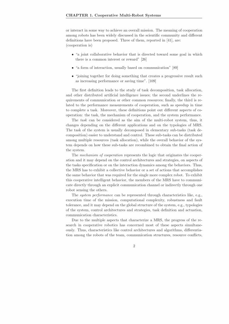
tion based on the typologies of vehicles and on their missions. The first applications
concerned systems made up of grounded mobile robots (e.g., see Figure 1.1), that
are autonomous robots with wheels or crawlers. Such robots can be built both for
indoor environments (i.e., buildings, museums and laboratories) [92, 68] or out-
door environments (i.e., open space with terrain, grass or rocky floor) [69, 42, 43]
and they result the most commonly used. However, in the latest years, applica-
tions with different kinds of vehicles have been proposed, e.g., different multi-robot
systems made up of Underwater Autonomous Vehicles (AUVs) [57, 121], control
techniques and experiments with aerial vehicles [29, 123, 72, 115, 30], and forma-
tion control with fleets of marine crafts [53, 120, 71].
The applications of multi-robot systems may involve different fields, e.g., indus-
trial, military and service robotics, or research and study of biological systems, and
they may concern largely different kind of missions, e.g., exploration, box push-
ing, military operation, navigation in unstructured environment, traffic control,
entrateinment, simulations of biological systems.
Several industrial applications, for example, concern the possibility to move
large objects using multiple robots (sometimes with manipulators on board). A
single robot, in fact, may be not enough powerful to push alone the object and it
can be unable to apply forces in all the generalized directions. Thus, a multi-robot
3

CHAPTER 1. Cooperative Multi-Robot Systems
Figure 1.1: Platoon of wheeled grounded mobile robots at the Laboratorio diAutomazione Industriale of the Universita degli Studi di Cassino
solution can be useful to share the needed power among multiple robots and, using
multiple contact points, it may permit to apply forces in the all generalized direc-
tions. On the other hand, the multi-robot solution needs for a strong coordination
among the robots, that means, the robots have to share information about their
relative positions and about the shape and position of the object. To achieve this
kind of mission (generally called Box-pushing Mission), different MRSs have been
presented, e.g., in [90] some experimental results of box pushing using two legged
robots are presented, in [136] a team of differential-drive mobile robots performs
the box-pushing mission without explicit communication, the work in [133] focuses
on function distribution and behavior design for cooperative object handling with
multiple mobile robots. Moreover, the work in [137] presents a motion-planning
method for multiple-mobile robots to cooperatively transport large objects, while,
finally, the work in [125] presents an approach to carry a deformable object by
means of two mobile robots with manipulators on board.
Another kind of application is the possibility to use a team of cooperating
robots to explore an unknown environment and build its map. To achieve this
mission in a cooperative way, the robots must be coordinated to explore different
parts of the environment and share partial maps elaborated by each single robot
to build the global map of the environment; as a consequence they can explore
the environment in less time than a single robot. Simultaneously, the robots have
4

1.2 Aims and Applications
a) b)
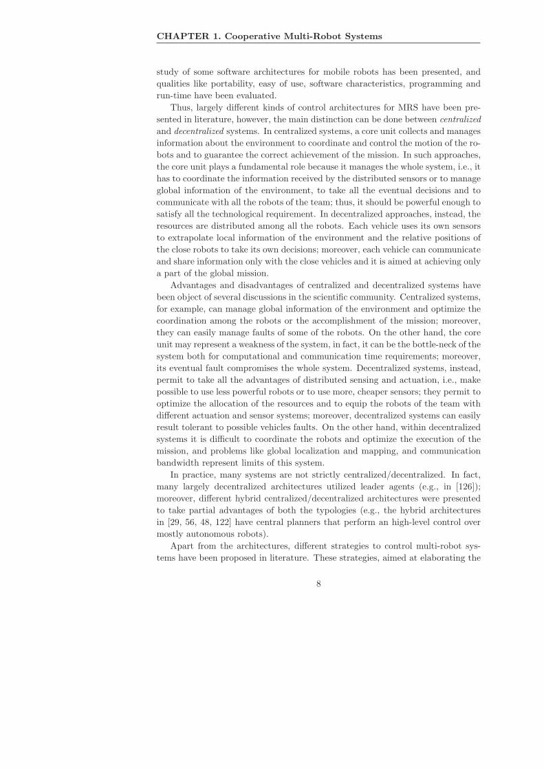
Figure 1.2: a) Fleet of marine surface vessels. b) Freccie Tricolore, Italian Acro-batic Air Force Unit.
to localize themselves with respect to the environment to correctly achieve the
mission and merge the partial maps. This kind of application, known in literature
as Simultaneous Localization And Mapping (SLAM), has been object of extensive
research efforts and different solutions have been proposed, e.g., in [110], a team
of two robots collaborate to explore and map a large environment and, sensing
one each other, try to reduce the odometric errors also coping with obstacles with
hard-to-sense reflectance characteristics. In [139], an approach for mapping and
exploration which exploits a market architecture in order to maximize information
gain while minimizing incurred cost is proposed. This system results reliable and
robust in that it can accommodate dynamic introduction and loss of team members
and it is able to withstand communication interruptions and failures. In [40],
experiments with a team of up to three heterogeneous robots is used to reduce
exploration time also in situation where the communication ranges of the robots
are limited. In the recent works [23, 24] a complete tutorial on SLAM for a single
autonomous robot is presented.
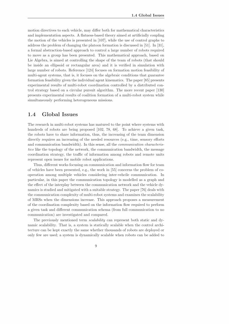
Part of the works in cooperative mobile robotics has a biological inspira-
tion (e.g., it is worth noticing the analogies among the manned fleets/flights in
Figure 1.2 and the biological system in Figure 1.3 while moving in formation).
This kind of approaches began after the introduction of the robotics paradigm of
behavior-based control [17, 39] that can be described by the relationship between
the 3 primitives of robotics: Sense, Plan, and Act. The behavior-based paradigm
for mobile robotics has been useful for robotics researchers to examine the social
characteristics of insects and animals, and to apply these findings to the design
of multi-robot systems. The most common application is the use of elementary
control rules of various biological animals (e.g., ants, bees, birds and fishes) to
reproduce a similar behavior (e.g., foraging, flocking, homing, dispersing [88]) in
5

CHAPTER 1. Cooperative Multi-Robot Systems
Figure 1.3: Birds flying in formation.
cooperative robotic systems. The first works have been motivated by application
in computer graphics, e.g., in 1986 Reynolds [111] made a computer model for co-
ordinating animal motion as bird flocks or fish schools. This pioneer work inspired
significant efforts in the study of group behaviors [99, 87, 79], then in the study
of multi-robot formations [132, 101, 25], till to fancy application like the sheep-
dog robot presented in [128]. However, the main behavior-based approaches will
be extensively discussed in Chapter 3 to introduce the behavior based technique
object of this thesis.
Another kind of application concerns the control of wireless Mobile Ad-hoc
NETworks (MANETs). In particular, the MANET is a collection of autonomous
nodes that communicate each other without using any fixed networking infrastruc-
ture. Each node in a MANET operates both as an host and as a router. Therefore,
any node can communicate directly with nodes that are within its transmission
range and, in order to reach a node that is out of its range, data packets are
relayed over a sequence of intermediate nodes using a store-and-forward multi-
hop transmission principle. The MANET approach is very attractive for on-field
mobile robots applications where often the task execution may compromise the
robot-base communication as, e.g., in a survey and rescue mission to be performed
inside a damaged building or in exploration of unknown areas. For this reason, a
number of researchers have started proposing MANET-based solutions for mobile
robot communication (e.g., see [47, 116, 134]). However, these solutions, as tra-
ditional MANET implementations, consider position and motion of each node as
uncontrollable variables. Assuming instead that at least some of the nodes may
be controlled, more performing MANETs can be designed. Indeed, a suitable dy-
namic reconfiguration of the robots’ position allows to adapt the coverage area of
the communication network to better support the team’s mission, to avoid signal
6

1.3 Control Architectures and Strategies
fading area (e.g., that induced by the presence of obstacles), and to handle pos-
sible fault of some team members. More details on MANET applications will be
presented in Section 5.2.
Several applications of multi-robot systems have been proposed also in the mil-
itary field [25, 93], e.g., for surveillance and rescue operations [43, 74]. Moreover,
in the last years, several research efforts have been direct towards the field of en-
trateinment; consider, for example, the vast development of soccer robots and the
advancement of the robocups [75, 96].
1.3 Control Architectures and Strategies
In the previous section, different kinds of applications for multi-robot systems
have been shown, however, nothing has been said about how to control a MRS
to achieve the different missions. The control architecture represents a central
part of the MRS because it determines the succes of the missions and it strongly
influences the global performance of the MRS.
Coordination and interaction of multiple intelligent agents have been actively
studied in the field of distributed artificial intelligence since the early 1970’s mainly
concerning problems involving software agents. Then, in the last 80’s early 90’s.,
the robotics research community became very active in the cooperative robotics
field with projects like CEBOT, SWARM, ACTRESS. In [64, 65], a distributed
hierarchical system (CEBOT) inspired by cellular organization of biological enti-
ties is presented. The CEBOT architecture is dynamically reconfigurable, that is,
the cells are able to communicate with each other, approach, connect and separate
automatically. Moreover, if a cell is damaged it can be automatically repaired or re-
placed to maintain the system functions. In [32], a distributed system with a large
number of autonomous robots (that in the follower works has been called SWARM)
is presented. With this architecture, also based on cellular robotic, the robots ac-
complish cooperation tasks like assembly, communication and computing. In [22],
an autonomous and distributed robotic system of multi robotic elements has been
presented. This work introduces an architecture, called ACTRESS, for hetero-
geneous robots that may differ both for structures and functions, and discusses
the communication protocol for cooperative actions between arbitrary elements.
All these projects concerned mostly simulations, while the implementations (with
few robots) were presented by way of proving the simulation results. More re-
cent works [99, 87, 132] are more significant to stress the implementation aspects
of cooperative robotic systems. In [100, 101], a behavior-based architecture for
cooperative control, called ALLIANCE, has been presented. The ALLIANCE ar-
chitecture has been developed in order to study cooperation in an heterogeneous,
small/midium size team of robots that should result in a fault tolerant, reliable
and adaptive mechanism for cooperative robot control. In [94], a comparative
7
CHAPTER 1. Cooperative Multi-Robot Systems
study of some software architectures for mobile robots has been presented, and
qualities like portability, easy of use, software characteristics, programming and
run-time have been evaluated.
Thus, largely different kinds of control architectures for MRS have been pre-
sented in literature, however, the main distinction can be done between centralized
and decentralized systems. In centralized systems, a core unit collects and manages
information about the environment to coordinate and control the motion of the ro-
bots and to guarantee the correct achievement of the mission. In such approaches,
the core unit plays a fundamental role because it manages the whole system, i.e., it
has to coordinate the information received by the distributed sensors or to manage
global information of the environment, to take all the eventual decisions and to
communicate with all the robots of the team; thus, it should be powerful enough to
satisfy all the technological requirement. In decentralized approaches, instead, the
resources are distributed among all the robots. Each vehicle uses its own sensors
to extrapolate local information of the environment and the relative positions of
the close robots to take its own decisions; moreover, each vehicle can communicate
and share information only with the close vehicles and it is aimed at achieving only
a part of the global mission.
Advantages and disadvantages of centralized and decentralized systems have
been object of several discussions in the scientific community. Centralized systems,
for example, can manage global information of the environment and optimize the
coordination among the robots or the accomplishment of the mission; moreover,
they can easily manage faults of some of the robots. On the other hand, the core
unit may represent a weakness of the system, in fact, it can be the bottle-neck of the
system both for computational and communication time requirements; moreover,
its eventual fault compromises the whole system. Decentralized systems, instead,
permit to take all the advantages of distributed sensing and actuation, i.e., make
possible to use less powerful robots or to use more, cheaper sensors; they permit to
optimize the allocation of the resources and to equip the robots of the team with
different actuation and sensor systems; moreover, decentralized systems can easily
result tolerant to possible vehicles faults. On the other hand, within decentralized
systems it is difficult to coordinate the robots and optimize the execution of the
mission, and problems like global localization and mapping, and communication
bandwidth represent limits of this system.
In practice, many systems are not strictly centralized/decentralized. In fact,
many largely decentralized architectures utilized leader agents (e.g., in [126]);
moreover, different hybrid centralized/decentralized architectures were presented
to take partial advantages of both the typologies (e.g., the hybrid architectures
in [29, 56, 48, 122] have central planners that perform an high-level control over
mostly autonomous robots).
Apart from the architectures, different strategies to control multi-robot sys-
tems have been proposed in literature. These strategies, aimed at elaborating the
8
1.4 Global Issues
motion directives to each vehicle, may differ both for mathematical characteristics
and implementation aspects. A flatness-based theory aimed at artificially coupling
the motion of the vehicles is presented in [107], while the use of control graphs to
address the problem of changing the platoon formation is discussed in [51]. In [31],
a formal abstraction-based approach to control a large number of robots required
to move as a group has been presented. This mathematical approach, based on
Lie Algebra, is aimed at controlling the shape of the team of robots (that should
be inside an ellipsoid or rectangular area) and it is verified in simulation with
large number of robots. Reference [124] focuses on formation motion feasibility of
multi-agent systems, that is, it focuses on the algebraic conditions that guarantee
formation feasibility given the individual agent kinematics. The paper [85] presents
experimental results of multi-robot coordination controlled by a distributed con-
trol strategy based on a circular pursuit algorithm. The more recent paper [130]
presents experimental results of coalition formation of a multi-robot system while
simultaneously performing heterogeneous missions.
1.4 Global Issues
The research in multi-robot systems has matured to the point where systems with
hundreds of robots are being proposed [102, 78, 68]. To achieve a given task,
the robots have to share information, thus, the increasing of the team dimension
directly requires an increasing of the needed resources (e.g., time, sensory efforts
and communication bandwidth). In this sense, all the communication characteris-
tics like the topology of the network, the communication bandwidth, the message
coordination strategy, the traffic of information among robots and remote units
represent open issues for mobile robot applications.
Thus, different works focusing on communication and information flow for team
of vehicles have been presented, e.g., the work in [55] concerns the problem of co-
operation among multiple vehicles considering inter-vehcile communication. In
particular, in this paper the communication topology is modelled as a graph and
the effect of the interplay between the communication network and the vehicle dy-
namics is studied and mitigated with a suitable strategy. The paper [76] deals with
the communication complexity of multi-robot systems and examines the scalability
of MRSs when the dimensions increase. This approach proposes a measurement
of the coordination complexity based on the information flow required to perform
a given task and different communication schema (from full communication to no
communication) are investigated and compared.
The previously mentioned term scalability can represent both static and dy-
namic scalability. That is, a system is statically scalable when the control archi-
tecture can be kept exactly the same whether thousands of robots are deployed or
only few are used; a system is dynamically scalable when robots can be added to
9
CHAPTER 1. Cooperative Multi-Robot Systems
or removed from the system on the fly; they may also have the ability to reallocate
and redistribute themselves in a self-organized way. The scalability properties can
be used as evaluation parameters for MRSs.
Moreover, among evaluation parameters, robustness, rather than efficiency, is
promoted. In fact, a multi-robot system may result robust to malfunctions like
unreliable communication and robot failures. Moreover, a MRS may be robust to a
priori unknown environmental and team changes not only through unit redundancy
but also through a balance between exploratory and exploitative behavior.
10

Chapter 2
Motion Control of
Autonomous Vehicles
Dealing with cooperative multi-robot systems, the most important requirement
is the motion coordination among the robots, that means, the robots have to
keep a suitable relative configuration during the whole mission. Thus, to correctly
achieve the coordination, it necessary to understand how to control the motion of
each single vehicle of the team.
Motion control is strictly related to the typology of the robots and to their kine-
matical and dynamical characteristics; in fact, wheeled robots (holonomic/non-
holonomic), marine surface vessels or underwater vehicles (totally or partially ac-
tuated) and aerial vehicles have different kinematical/dynamical characteristics
and may give rise to different control problems. The literature in the field is
vast, thus, without having the scope of a survey, in this chapter, the only basic
motion control aspects that are functional for the remaining part of this thesis
will be presented and discussed. In particular, because the control strategy pre-
sented in the next chapters have been tested with differential-drive mobile robots
and fully/under-actuated marine surface vessels, this chapter will focus only on
wheeled mobile robots and marine vessels.
However, to have an overview of the main aspects of motion control for dif-
ferent kind of vehicles, the reader can look through the few references listed in
the following. In [118], an introduction to the main topics of mobile robotics is
presented; in [81], the main aspects of motion planning of autonomous robot are
illustrated; the paper [77] presents a survey on non-holonomic control problems
while the book [35] deals with mathematical details of control theory for non holo-
nomic mechanical systems. The book [59] presents an overview on the control
of marine systems while the book [58], and more recently the book [2], present
overviews on the control of underwater robots.
11
CHAPTER 2. Motion Control of Autonomous Vehicles
a) b)
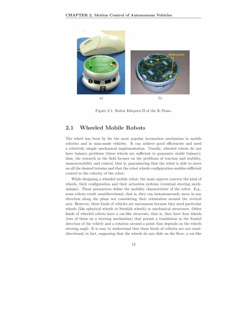
Figure 2.1: Robot Khepera II of the K-Team.
2.1 Wheeled Mobile Robots
The wheel has been by far the most popular locomotion mechanism in mobile
robotics and in man-made vehicles. It can achieve good efficiencies and need
a relatively simple mechanical implementation. Usually, wheeled robots do not
have balance problems (three wheels are sufficient to guarantee stable balance),
thus, the research in the field focuses on the problems of traction and stability,
maneuverability and control, that is, guaranteeing that the robot is able to move
on all the desired terrains and that the robot wheels configuration enables sufficient
control to the velocity of the robot.
While designing a wheeled mobile robot, the main aspects concern the kind of
wheels, their configuration and their actuation systems (eventual steering mech-
anisms). These parameters define the mobility characteristic of the robot. E.g.,
some robots result omnidirectional, that is, they can instantaneously move in any
direction along the plane not considering their orientation around the vertical
axis. However, these kinds of vehicles are uncommon because they need particular
wheels (like spherical wheels or Swedish wheels) or mechanical structures. Other
kinds of wheeled robots have a car-like structure, that is, they have four wheels
(two of them on a steering mechanism) that permit a translation in the frontal
direction of the vehicle and a rotation around a point that depends on the wheels
steering angle. It is easy to understand that these kinds of vehicles are not omni-
directional; in fact, supposing that the wheels do not slide on the floor, a car-like
12

2.1 Wheeled Mobile Robots
robot can not translate in its lateral direction. The most popular kind of mobile
robot is the two-wheel differential-drive robot (e.g., see Figure 2.1), that is, a robot
with two wheels actuated by two independent motors with a coincident rotation
axis. However, because the mobile robots need three ground contact points for the
balance, for differential-drive robot, one or two additional passive castor wheels
(i.e., free wheels rotating around a vertical axis) or slider points (see Figure 2.1.b)
may be used for stability.
2.1.1 Kinematic Model of Differential-Drive Robot
Deriving a model for the robot’s motion is a bottom up process. Each individual
wheel contributes to the robot motion and, at the same time, imposes constraints
on it. Thus, the constraints of each wheel combine to form the constraints of the
overall motion of the robot.
YI
XI
XR
YR
θ
P
0 x
y
Figure 2.2: Global reference frame and robot local reference frame.
To model the motion of the mobile robot, the constraints and the forces of
each wheel must be expressed respect to a proper and consistent reference frame.
Thus, to specify the robot position, it is possible to consider the robot as a rigid
body on wheels operating on an horizontal plane, and to consider its three Degrees
Of Freedom (DOF) (two for the horizontal position in the plane and one for the
orientation around a vertical axis). Then, the position of the robot can be specified
by the relationship between a global inertial reference frame and a body-fixed
reference frame. E.g., in Figure 2.2 the axes XI and YI define an inertial reference
frame, while the axes XR and YR define a body-fixed reference frame. The position
of the robot is specified by the coordinates x and y of the point P in the {XI , YI}
13

CHAPTER 2. Motion Control of Autonomous Vehicles
frame, and by the angle θ between the axes XI and XR:
P I =
xyθ
. (2.1)
In the general case, the motion of the robot is described by the equations:
x = u cos (θ) − v sin (θ) (2.2)
y = u sin (θ) + v cos (θ) (2.3)
θ = ω (2.4)
or in compact form:
P I = R (θ)
uvω
(2.5)
where u, v are the components of the linear velocity in a reference frame instanta-
neously superimposed to the body-fixed reference frame, ω is the angular velocity
and R is the orthogonal rotation matrix defined as:
R (θ) =
cos (θ) − sin (θ) 0sin (θ) cos (θ) 0
0 0 1
. (2.6)
In case of differential-drive robots (as in Figure 2.2), assuming that the two
wheels roll without slipping on the floor, then, the velocity components are:
u = (ωrr + ωlr) /2 (2.7)
ω = (ωrr − ωlr) /l (2.8)
where ωr, ωl are the angular velocities of the right/left wheels, r is the wheels’
radius and l is the distance between the wheels.
Thus, the overall motion of the robot is described by two instantaneous ele-
mentary motions: the translation in the XI direction and the rotation around a
vertical axis through the point P . Moreover, the component v of the linear veloc-
ity (i.e., the translation in the lateral direction) is null and the motion equations
are simplified to:
x = u cos (θ) (2.9)
y = u sin (θ) (2.10)
θ = ω. (2.11)
It is worth noticing that the two-wheel differential-drive robot has a kinematical
structure analogous to the unicycle (also known as vertical rolling disk, see [35]),
that is, an homogeneous disk that rolls without slipping on an horizontal plane
(see Figure 2.3). The unicycle, in fact, has a kinematical model described by the
same equations of 2.9 - 2.11 .
14

2.1 Wheeled Mobile Robots
Figure 2.3: Vertical rolling disk.
2.1.2 Motion Control for Nonholonomic Systems
The basic motion tasks considered for a grounded mobile robot in an obstacle-free
environment are the following:
• point-to-point motion: a desired goal configuration must be reached starting
from a given initial configuration;
• trajectory following: a reference point on the robot must follow a trajectory
in the Cartesian space (i.e., a geometric path with an associated timing law)
starting from a given initial configuration.
The execution of these tasks can be achieved using either feedforward or feed-
back control (or a combination of the two); obviously, the latter has to be preferred
in view of its intrinsic degree of robustness. When executed under a feedback
strategy, the point-to-point motion task leads to a regulation control problem for
a point in the robot state space. Instead, trajectory following leads naturally to a
tracking problem, which may be asymptotic in the presence of an initial error (i.e.,
an off-trajectory start for the vehicle). The term trajectory tracking is adopted
referring to the problem of stabilizing to zero the two-dimensional Cartesian error
with respect to the position of a moving reference robot.
From a mathematical point of view, the not slipping condition of the non-
omnidirectional wheeled robots results in a kinematic constraint represented by
a differential relationship. This kind of constraint cannot be integrated and, in
these systems, it is not possible to choose generalized coordinates equal to the
number of DOFs. I.e., the number of generalized (e.g., Lagrangian) coordinates
exceeds the number of degrees of freedom by the number of independent, nonin-
tegrable constraints. Such systems are called nonholonomic and they present an
15

CHAPTER 2. Motion Control of Autonomous Vehicles
adjunct complexity for the control system because such systems cannot be stabi-
lized at a point by smooth feedback [49]. Thus, the design of posture stabilization
laws for nonholonomic systems has to face a serious structural obstruction. As
a consequence, opposite to the usual situation, tracking is easier than regulation
for a nonholonomic vehicle. However, several alternative approaches have been
proposed for regulation of nonholonomic systems.
The simplest approach to designing feedback controllers for nonholonomic sys-
tems is probably to decompose the control in two stages: first, find an open-loop
strategy that can achieve any desired reconfiguration for the particular system
under consideration. Second, transform the motion sequence into a succession of
equilibrium manifolds, which are then stabilized by feedback. The overall resulting
feedback is necessarily discontinuous, because of the switching of the target man-
ifolds. Each stabilization problem in the succession should be completed in finite
time (that is, not just asymptotically), so as to have a well-defined procedure. In
order to achieve such convergence behavior, discontinuous feedback is used within
each stabilizing phase. The weakness of this approach is that it requires the abil-
ity to devise an openloop strategy for the system. Moreover, any perturbation
occurring on a variable that is not directly controlled during the current phase
will result in a final error. As a result, feedback robustness is achieved only with
respect to perturbation of the initial conditions.
Another approach is to use a time-varying controller. The idea of allowing the
feedback law to depend explicitly on time is due to Samson [113], who presented
smooth stabilization schemes for the car-like kinematic models. When considering
the point-stabilization of a time-invariant nonholonomic system, the introduction
of a time-varying component in the control law may lead to a smoothly stabilizable
system. However, these time-varying control laws have typically slow rates of
convergence and a difficult tuning of the various parameters of the controller. An
experimental validation of these kind of controllers can be found in [73].
An hybrid strategy for the stabilization of the unicycle has been proposed in
[108], namely, combining the advantages of smooth static feedback far from the
target and time-varying feedback close to the target.
2.2 Marine Surface Vessels
As reported in [59], the history of model based ship control starts with the in-
vention of the gyrocompass in 1908, and it extends further with the development
of local positioning systems in the 1970s. Global coverage using satellite navi-
gation systems was first made available in 1994. The gyrocompass was the basic
instrument in the first feedback control system for heading control and today these
devices are known as autopilots. Feedback control applications to marine vessels
have became more and more popular thanks to the developments in computer sci-
16
2.2 Marine Surface Vessels
ence, propulsion systems and modern sensor technology. Examples of commercial
available systems are:
• ships and underwater autopilots for course-keeping and turning control;
• way-point tracking, trajectory and path control systems for marine vessels;
• dynamic positioning systems for marine vessels;
• propulsion control system and forward speed control.
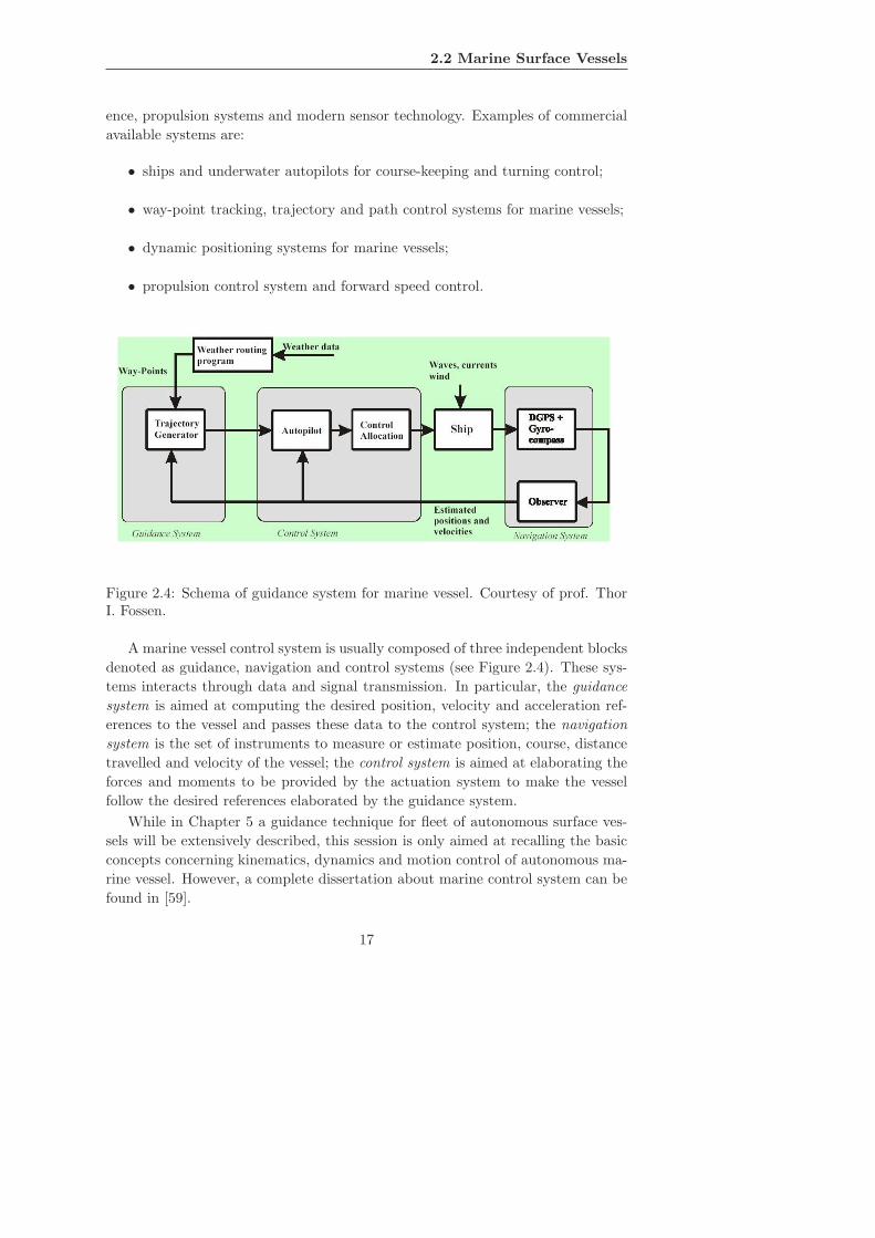
Figure 2.4: Schema of guidance system for marine vessel. Courtesy of prof. ThorI. Fossen.
A marine vessel control system is usually composed of three independent blocks
denoted as guidance, navigation and control systems (see Figure 2.4). These sys-
tems interacts through data and signal transmission. In particular, the guidance
system is aimed at computing the desired position, velocity and acceleration ref-
erences to the vessel and passes these data to the control system; the navigation
system is the set of instruments to measure or estimate position, course, distance
travelled and velocity of the vessel; the control system is aimed at elaborating the
forces and moments to be provided by the actuation system to make the vessel
follow the desired references elaborated by the guidance system.
While in Chapter 5 a guidance technique for fleet of autonomous surface ves-
sels will be extensively described, this session is only aimed at recalling the basic
concepts concerning kinematics, dynamics and motion control of autonomous ma-
rine vessel. However, a complete dissertation about marine control system can be
found in [59].
17

CHAPTER 2. Motion Control of Autonomous Vehicles
2.2.1 Kinematics
In maneuvering, a marine vessel experiences motion in 6 degrees of freedom (see
Figure 2.5). The motion in the horizontal plane is referred to as surge (longitudinal
motion) and sway (sideways motion), while the motion in the vertical direction is
referred to as heave. Heading or yaw (rotation around the vertical axis) describes
the course of the vessel in the horizontal plane, while roll and pitch represent
respectively the rotations around longitudinal and transverse axis.
Figure 2.5: Elementary motions of a marine vessel respect to a body-fixed referenceframe. Courtesy of prof. Thor I. Fossen.
Describing the motion of the vessel, the first step is to define the reference
frames. For marine vessel operating in a local area, usually a flat Earth model
is used for the navigation and a North-East-Down (NED) reference system is
used as inertial reference frame. In the NED reference system, the x-axis points
towards North, y-axis points towards East and z-axis points downwards normal to
the Earth surface. A body-fixed reference frame (BODY) is a moving coordinate
frame, fixed to the vessel, that is usually chosen as in Figure 2.5. Thus, the position
and orientation of the vessel is described by the relative position p and orientation
Θ (Euler’s angles Roll, Pitch and Yaw) of the BODY respect to the NED:
BODY position: p =
xyz
BODY orientation: Θ =
φθψ
The vessel velocity is described by the components of the linear velocity v and
angular velocity ω respect to a reference system instantaneously superimposed to
the BODY:
18

2.2 Marine Surface Vessels
Linear velocity in BODY: v =
uvw
Angular velocity in BODY: ω =
pqr
In the case of marine surface vessels, the motion is supposed in the horizontal plane
and is described by the only surge, sway and yaw components. Thus, assuming
w = p = q = 0 and defining ν = [u, v, r] and η = [x, y, ψ] the kinematic model of
the surface vessel (see Figure 2.6) is described by the relation:
η = R(ψ)ν (2.12)
where R(ψ) ∈ SO(3) is the rotation matrix from NED to BODY (that describes
a pure rotation around the z-axis):
R (θ) =
cos (ψ) − sin (ψ) 0sin (ψ) cos (ψ) 0
0 0 1
. (2.13)
N ≡ X
E ≡ Y
ψ
xb
yb
{B}x
y
Figure 2.6: NED and BODY reference frame for a marine surface vessel.
2.2.2 Dynamics
By Newton’s second law, it is shown in [59] that the vessel dynamic equation can
be written as
Mν + C(ν)ν + D(ν)ν = τ + RT(ψ)w, (2.14)
where M is the vessel inertia matrix with added mass; C(ν) is the centrifugal and
Coriolis matrix with added mass; D(ν) the hydrodynamic damping matrix; τ is
the vessel propulsion force and torque; w is the vector of the environmental forces
(wind, currents, etc.) acting on the vessel in the NED reference system.
19
CHAPTER 2. Motion Control of Autonomous Vehicles
Assuming that the origin of the BODY is in the geometric center of the vessel,
that the vessel is port-starboard symmetric with an homogeneous mass distrib-
ution, then, the center-of-gravity will be located a distance xg along the body
x-axis, and the inertia matrix M becomes:
M =
m−Xu 0 0
0 m− Yv mxg − Yr
0 mxg − Yr Iz −Nr
. (2.15)
where m is the mass of the vessel, Iz is the moment of inertia around the z-axis
and Xu, Yv, Yr, Nr are the added mass parameters. Moreover, the Coriolis matrix
C becomes:
C (ν) =
[0 0 −(m − Yv)v − (mxg − Yr)r0 0 (m − Xu)u
(m − Yv)v + (mxg − Yr)r −(m − Xu)u 0
],
(2.16)
while the linear damping matrix D (i.e., neglecting the non linear terms) becomes:
D (ν) =
−Xu 0 00 −Yv −Yr
0 −Nv −Nr
. (2.17)
2.2.3 Motion Control
Also for the case of marine surface vessels, the basic motion tasks are the following:
• point-to-point motion: a desired goal configuration must be reached starting
from a given initial configuration;
• trajectory following: a reference point on the vessel must follow a trajectory
in the Cartesian space (i.e., a geometric path with an associated timing law)
starting from a given initial configuration.
Depending on the characteristics of the generalized propulsion force applied by
the actuation system (represented by the vector τ of eq. (2.14)), the vessels can
be classified in fully-actuated and under-actuated. In detail, the vessel is fully-
actuated when the propulsive action can span all the generalized directions (i.e.,
both forces in the surge and sway directions and torque in the yaw direction can
be applied), otherwise it is underactuated (e.g., less than three actuators are used
to control the surge, sway and yaw motions). Motion control characteristics for
these two typologies of vehicles are widely different because under-actuated vessels
present an adjunct control complexity. That is, the under-actuation results in an
second-order constraint that may give integrability problems (analogously to the
case of nonholonomic systems), as explained in [135]. The reader can look through
the works in [103, 82, 104] to have an overview of the main control problems
regarding underactuated ships.
20

2.2 Marine Surface Vessels
In marine applications, the point-to-point motion is overall focused on keeping
a certain fixed position while performing a low-speed maneuvering. The con-
trol systems aimed at this purpose are usually called Dynamic Positioning (DP)
systems. In particular, a dynamically positioned vessel is a free-floating vessel
which maintains its position (i.e., the three horizontal motions surge, sway and
yaw) exclusively by mean of thrusters. Several approaches have been presented to
achieve the DP controls by mean of different actuation systems (e.g., the DP sys-
tem for underactuated vessels presented in [103]), considering the environmental
conditions (e.g., the weather optimal positioning control in [63]) and the available
measurements (e.g., the DP with only position measurements proposed in [83]).
The trajectory following controller, also called maneuvering control, is a on
board controller aimed at steering the vessel along a desired path and moving it
with a desired velocity [59, 60]. For fully actuated ships, the maneuvering control
problem has been extensively explained in [119]. For underactuated ships, the
maneuvering control is a challenging problem; however, several works have been
presented in literature, e.g., the tracking control proposed in [82] and the line-of-
sight path following approach proposed in [61].
21
CHAPTER 2. Motion Control of Autonomous Vehicles
22
Chapter 3
The Null-Space-Based
Behavioral Control
Once introduced the main concepts concerning multi-robot systems and motion
control of single autonomous vehicles, in this chapter, a behavior based technique,
namely the Null-Space-based Behavioral control (NSB), to control both single au-
tonomous vehicles and multi-robot systems will be presented. In particular, the
NSB will be introduced in its mathematical details and, to better underline its
characteristics, it will be presented in an unified framework together with two
of the main behavioral approaches; namely, the layered control system [39] as a
significant case of competitive approach and the motor schema control [17] as a
significant case of cooperative approach. To allow a clear comparison, consider-
ing the same set of tasks for all these approaches, the different mechanisms to
compose the velocity commands to the robots, starting from the outputs of each
elementary task, will be discussed. The comparison will be experimentally vali-
dated performing with all the approaches the same mission of reaching a target
avoiding an obstacle. Finally, the use of the NSB to control a single vehicle while
kicking a ball will be presented.
3.1 Behavioral Approaches
As previously introduced, autonomous robots pose challenging control problems.
They need to process many data in real-time, eventually working in an unstruc-
tured environment, while accomplishing several tasks such as manipulation, ex-
ploration, mapping, or moving through predefined via-points. Obviously, they
need also to avoid static or dynamic obstacles, perform fault detection algorithms
and preserve their integrity. An autonomous robot, thus, needs to achieve several
goals at the same time; these may conflict one with the other and a relative impor-
tance among them is to be assigned. Moreover, the importance of a goal is often
23
CHAPTER 3. The Null-Space-Based Behavioral Control
context-depend; for example, obstacle avoidance of a static, far, obstacle might be
of smaller importance with respect to the goal of reaching a close target position.
As recognized in [39], performing these operations in a pure serial sequence
is a debatable approach. The most promising approach seems instead to decom-
pose the problem in several sub-problems, eventually solvable in parallel, whose
solutions then need to be composed in one single motion command to the robot.
The sub-problems are commonly termed behaviors, functional modules, motor
schemes, or tasks and these terms will be used as synonyms in this thesis while
calling in short behavioral approach any method aimed at properly composing the
elementary behaviors.
Among the behavioral approaches, seminal works are reported in the pa-
pers [39] and [17], while the textbook [18] offers a comprehensive state of the art.
A behavioral approach designed for exploration of planetary surfaces has been in-
vestigated in [66], while, in [80], the experimental case of an off-road navigation is
presented. Lately, behavioral approaches have been applied to the formation con-
trol of multi-robot systems as in, e.g. [101, 89, 25]. The use of techniques inherited
from inverse kinematics for industrial manipulators is described in [33, 13, 138].
In [112], a hierarchical behavior-based system that performs several vision-based
manipulation tasks by using different combinations of the same set of basic be-
haviors has been presented. In [114], an architecture for dynamic changes of the
behavior selection strategies has been presented.
Usually, a behavior is expressed through a function of the robot configuration
that measures the degree of fulfilment of the task (e.g., a cost or a potential
function); thus, in a static environment the task is achieved when its output is
constant at a value that minimizes the task function. For example, if the task
output is a velocity command to a mobile robot, to reach a given goal position
a distance-from-goal task function can be considered; the velocity command will
then be generated so as to reduce the distance between the vehicle and the goal,
and it will be null when the goal position is reached. Furthermore, if an obstacle
must be avoided, another velocity command will be generated so as to increase
the distance between the vehicle and the obstacle; this command will be null
when the obstacle is considered out of reach. In this scenario, when the obstacle
is somewhere along the line of sight of the goal position from the robot the two
behaviors come in conflict: in fact, the two individual-task velocity commands will
counteract and the vehicle can either approach the goal position (and come closer
to the obstacle too) or escape the obstacle (and drive away from the goal position
too).
The behavioral approaches differ in the way they compose the single task out-
puts to build the motion command to the robot. In presence of multiple behaviors,
each task output is designed so as to achieve its specific goal but it is generally
impossible that a single motion command to the robot can accomplish all the as-
signed behaviors at the same time. In particular, when a motion command cannot
24
3.1 Behavioral Approaches
reduce simultaneously the value of all the task functions there is a conflict among
the tasks that must be solved by a suitable policy. Thus, one important feature
that characterizes the behavioral approaches is the way they handle multiple ele-
mentary tasks to be achieved simultaneously. From a general point of view, the
different solutions to this problem of behavioral coordination can be basically cast
either in the frame of competitive methods or in the frame of cooperative meth-
ods [18]. In the competitive methods at each time instant only one task is selected
to be active and the control algorithm tries to solve only the chosen task. In the
cooperative methods, instead, a supervisor elaborates each elementary task as if
it were alone and builds the overall solution as the weighted sum of all the mo-
tion commands resulting from the single elementary tasks; in addition, on the the
basis of sensory information, the supervisor can dynamically change the relative
importance of the tasks by changing the vector of weight gains.
3.1.1 Competitive Behaviors Coordination
Competitive methods provide a means of coordinating behavioral response for con-
flict resolution. The coordination can be viewed as a competition among behaviors;
only one behavior wins and its response only is sent to the robot for execution.
This type of competitive strategy can be performed in a variety of ways. Gen-
erally, a coordination function (serving as an arbiter) selects a single behavioral re-
sponse. The function can take the form of either a prioritization network (in which
a strict behavioral dominance hierarchy exists) or an action-selection method (in
which, on the basis of sensor information, only the most active behavior is se-
lected).
sensorsTask
actuators
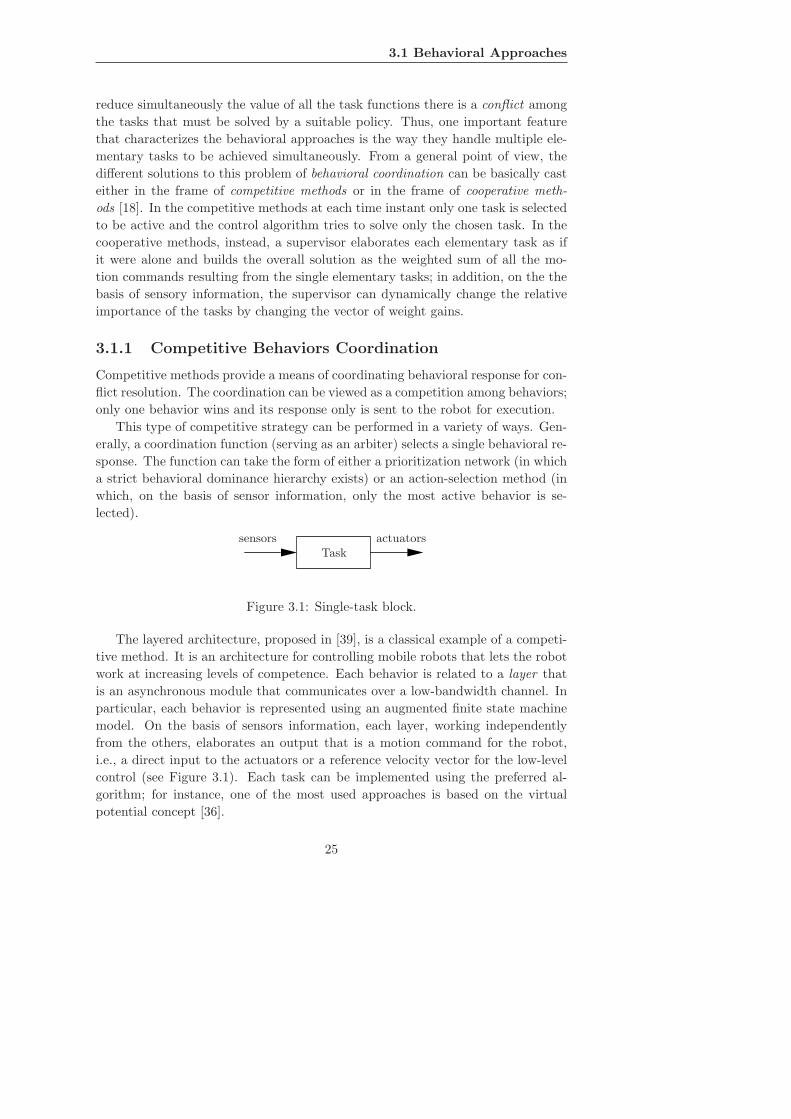
Figure 3.1: Single-task block.
The layered architecture, proposed in [39], is a classical example of a competi-
tive method. It is an architecture for controlling mobile robots that lets the robot
work at increasing levels of competence. Each behavior is related to a layer that
is an asynchronous module that communicates over a low-bandwidth channel. In
particular, each behavior is represented using an augmented finite state machine
model. On the basis of sensors information, each layer, working independently
from the others, elaborates an output that is a motion command for the robot,
i.e., a direct input to the actuators or a reference velocity vector for the low-level
control (see Figure 3.1). Each task can be implemented using the preferred al-
gorithm; for instance, one of the most used approaches is based on the virtual
potential concept [36].
25

CHAPTER 3. The Null-Space-Based Behavioral Control
Layers have different priority levels and the possible conflict among the tasks
is solved by assigning a hierarchy so that the higher-level tasks can subsume the
lower-level ones. This architecture, also known in literature as subsumption archi-
tecture, needs the use of a priority-based coordination function. From a practical
aspect, the subsumption can follow two mechanisms: the inhibition, used to pre-
vent that a signal is transmitted to the actuators, and the suppression, in which a
signal is replaced by an higher-priority one.
sensorsTask #2
v2
Task #1v1
Task #3v3 vd
Figure 3.2: Sketch of the layered control system in a 3-task example.
Figure 3.2, reproduced from [39], represents the functional scheme of this sub-
sumption architecture in a 3-task example. It is interesting to notice that no higher
level supervisor is required since each task can subsume the lower level ones and,
if not subsumed by an other higher level, directly commands the actuators.
With this approach, only the higher active task is properly achieved and it is
possible to add new layers simply choosing their positions in the hierarchy. Only
when the higher-priority task is fulfilled, by outputting a zero motion command
and not subsuming the lower-priority tasks, the second-highest in the hierarchy
starts to be satisfied. The tasks, thus, are pursued selectively based on the available
sensorial information.
In the older version of this algorithm the overall robot behavior is simply
achieved by collecting elementary behaviors; later, an intermediate level has been
proposed and the overall robot behavior is obtained by selecting an abstract be-
havior that is, itself, a collection of elementary behaviors ([18]).
3.1.2 Cooperative Behaviors Coordination
Cooperative methods provide an alternative to competitive. Behavioral fusion
provides the ability to concurrently use the output of more than one behavior at a
time. A supervisor elaborates each behavior and gives as output an intermediate
solution, calculated as the sum of all the motion commands (one for each task)
opportunely multiplied by a gain vector. The supervisor, on the basis of sensor
26
3.1 Behavioral Approaches
sensorsTask #2
v2 ⊗
α2
Task #1v1
supervisor
⊗
α1
Task #3v3 ⊗
α3
∑ vd
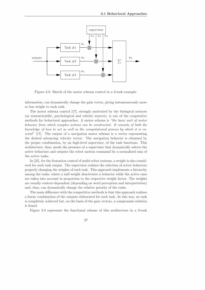
Figure 3.3: Sketch of the motor schema control in a 3-task example.
information, can dynamically change the gain vector, giving instantaneously more
or less weight to each task.
The motor schema control [17], strongly motivated by the biological sciences
(as neuroscientific, psychological and robotic sources), is one of the cooperative
methods for behavioral approaches. A motor schema is “the basic unit of motor
behavior from which complex actions can be constructed. It consists of both the
knowledge of how to act as well as the computational process by which it is en-
acted” [17]. The output of a navigation motor schema is a vector representing
the desired advancing velocity vector. The navigation behavior is obtained by
the proper combination, by an high-level supervisor, of the task functions. This
architecture, thus, needs the presence of a supervisor that dynamically selects the
active behaviors and outputs the robot motion command by a normalized sum of
the active tasks.
In [25], for the formation control of multi-robot systems, a weight is also consid-
ered for each task output. The supervisor realizes the selection of active behaviors
properly changing the weights of each task. This approach implements a hierarchy
among the tasks, where a null weight deactivates a behavior while the active ones
are taken into account in proportion to the respective weight factor. The weights
are usually context-dependent (depending on word perception and interpretation)
and, thus, can dynamically change the relative priority of the tasks.
The main difference with the competitive methods is that this approach realizes
a linear combination of the outputs elaborated for each task. In this way, no task
is completely achieved but, on the basis of the gain vectors, a compromise solution
is found.
Figure 3.3 represents the functional scheme of this architecture in a 3-task
27

CHAPTER 3. The Null-Space-Based Behavioral Control
example; with respect to the subsumption architecture in Figure 3.2 the main
difference is in the presence of a supervisor. As well as in the layered control
system, each task can be implemented using the preferred algorithm, e.g., the
virtual potential approach [17, 36].
3.2 NSB Mathematics
As discussed in the previous section, in a general robot mission the accomplishment
of several tasks at the same time is of interest. A possible technique to handle
the tasks’ composition has been proposed in [33, 34], which consists in assigning a
relative priority to the single task functions by resorting to the task-priority inverse
kinematics introduced in [84, 91] for ground-fixed redundant manipulators.
In [34], a kinematic control approach is used: the reference velocities pro-
vided by different inverse kinematic functions, however, are simply added one each
other. The overall algorithm performance, thus, is close to that of a behavioral
approach [25]. In detail, according to the reference [34], multiple tasks are handled
with only two priority levels; therefore, there can be different tasks at the same
priority level whose possible conflicts cannot be handled. Similarly, in [122], a par-
tially decentralized strategy based on the concept of kinematic control has been
proposed; the controller pursues a primary task that combines multiple objectives
and uses in proximity of obstacles a null-space projection to locally achieve their
avoidance. While both these papers use a null-space projection, they don’t fully
implement a task-priority approach; in fact, the combination of different tasks
at the same level of priority is a task-augmentation strategy that requires struc-
turally compatible tasks. For this reason, these approaches are not robust to the
occurrence of algorithmic singularities [45].
To manage multiple tasks, a task-priority approach, which is a well known
technique for inverse kinematics of ground-fixed manipulators [91], has been con-
sidered. In particular, the task priority method allows one to properly handle the
conflicts among different tasks that give rise to the so-called algorithmic singular-
ities, i.e., the single tasks are well defined and feasible but their combination leads
to a singular augmented Jacobian. The problems related to both kinematic and
algorithmic singularities have been deeply discussed in [45], where a singularity-
robust task-priority strategy, which is the basis of the technique presented in this
thesis, has been derived. It is worth recalling that, through a null-space projection,
a secondary task is fulfilled if it does not conflict with the primary task, while it
is released in case of conflict. One benefit of the singularity robustness shown by
the adopted algorithm is the possibility to design complex missions with several
tasks hierarchically arranged.
Based on these works, this idea has been developed in [13] in the framework
of the singularity-robust task-priority inverse kinematics [45]. In [15, 16], this
28

3.2 NSB Mathematics
approach has been used in simulation to control a multi-robot team performing a
caging mission, subject to obstacle avoidance and failure of one or more vehicles.
With reference to a generic platoon of autonomous vehicles (as shown [7]), the
basic concepts are recalled in the following.
Let define the position of the i-th vehicle as
pi = [xi yi zi ]T
and its linear velocity as
vi = [ xi yi zi ]T,
where xi, yi, and zi are the i-th vehicle’s coordinates with respect to an inertial
reference frame and the dot symbol represents the time derivative. To keep the
notation compact it is also useful to define the vectors p ∈ IR3n as
p = [pT1 . . . pT
n ]T
and v ∈ IR3n as
v = [vT1 . . . vT
n ]T.
By defining as σ∈ IRm the task variable to be controlled, it is:
σ = f(p) (3.1)
with the corresponding differential relationship:
σ =∂f(p)
∂pv = J(p)v , (3.2)
where J ∈ IRm×n is the configuration-dependent task Jacobian matrix. Notice
that n depends on the specific robotic system considered, in case of a differential
mobile robot n = 3, and the term system configuration simply refers to the robot
position/orientation, in case of a full actuated underwater vehicle n = 6, finally,
an anthropomorphic robots can reach very large value of n.
An effective way to generate motion references pd,i(t) for the vehicles starting
from desired time history σd(t) of the task function is to act at the differential
level by inverting the (locally linear) mapping (3.2); in fact, this problem has been
widely studied in robotics (see, e.g., [117] for a tutorial). For matrices with more
columns than rows —which is usually the case in Multi-Robot System control,
being 3n ≫ m— the problem admits infinite solutions and such redundancy is
often exploited to optimize some criterion. A typical requirement is to pursue
minimum-norm velocity, leading to the least-squares solution:
vd = J†σd = JT(JJT
)−1
σd . (3.3)
At this point, the vehicle motion controllers need reference position trajectories
besides the velocity references; these can be obtained by time integration of vd.
29
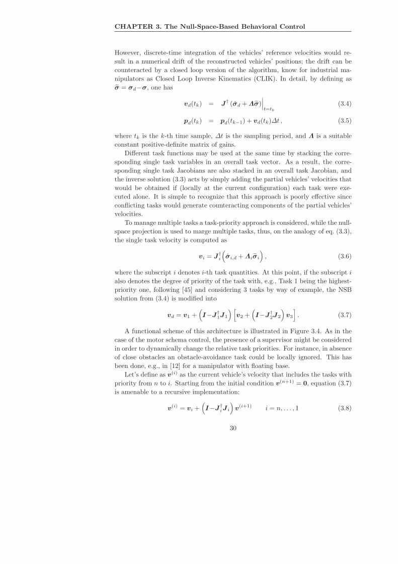
CHAPTER 3. The Null-Space-Based Behavioral Control
However, discrete-time integration of the vehicles’ reference velocities would re-
sult in a numerical drift of the reconstructed vehicles’ positions; the drift can be
counteracted by a closed loop version of the algorithm, know for industrial ma-
nipulators as Closed Loop Inverse Kinematics (CLIK). In detail, by defining as
σ = σd−σ, one has
vd(tk) = J† (σd + Λσ)∣∣∣t=tk
(3.4)
pd(tk) = pd(tk−1) + vd(tk)∆t , (3.5)
where tk is the k-th time sample, ∆t is the sampling period, and Λ is a suitable
constant positive-definite matrix of gains.
Different task functions may be used at the same time by stacking the corre-
sponding single task variables in an overall task vector. As a result, the corre-
sponding single task Jacobians are also stacked in an overall task Jacobian, and
the inverse solution (3.3) acts by simply adding the partial vehicles’ velocities that
would be obtained if (locally at the current configuration) each task were exe-
cuted alone. It is simple to recognize that this approach is poorly effective since
conflicting tasks would generate counteracting components of the partial vehicles’
velocities.
To manage multiple tasks a task-priority approach is considered, while the null-
space projection is used to marge multiple tasks, thus, on the analogy of eq. (3.3),
the single task velocity is computed as
vi = J†i
(σi,d + Λiσi
), (3.6)
where the subscript i denotes i-th task quantities. At this point, if the subscript i
also denotes the degree of priority of the task with, e.g., Task 1 being the highest-
priority one, following [45] and considering 3 tasks by way of example, the NSB
solution from (3.4) is modified into
vd = v1 +(I−J
†1J1
) [v2 +
(I−J
†2J2
)v3
]. (3.7)
A functional scheme of this architecture is illustrated in Figure 3.4. As in the
case of the motor schema control, the presence of a supervisor might be considered
in order to dynamically change the relative task priorities. For instance, in absence
of close obstacles an obstacle-avoidance task could be locally ignored. This has
been done, e.g., in [12] for a manipulator with floating base.
Let’s define as v(i) as the current vehicle’s velocity that includes the tasks with
priority from n to i. Starting from the initial condition v(n+1) = 0, equation (3.7)
is amenable to a recursive implementation:
v(i) = vi +(I−J
†iJ i
)v(i+1) i = n, . . . , 1 (3.8)
30
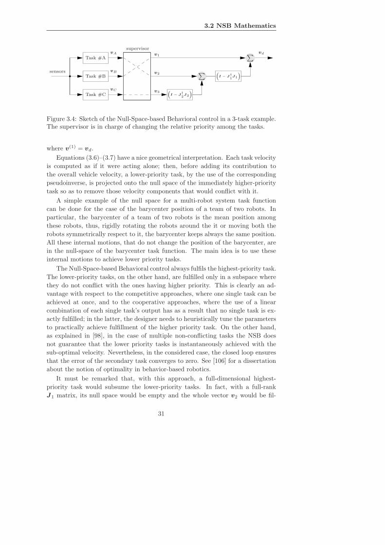
3.2 NSB Mathematics
sensors
Task #CvC v3
(I − J
†
2J2
)
Task #BvB v2
∑ (I − J
†
1J1
)
Task #AvA v1
∑ vd
supervisor
Figure 3.4: Sketch of the Null-Space-based Behavioral control in a 3-task example.The supervisor is in charge of changing the relative priority among the tasks.
where v(1) = vd.
Equations (3.6)–(3.7) have a nice geometrical interpretation. Each task velocity
is computed as if it were acting alone; then, before adding its contribution to
the overall vehicle velocity, a lower-priority task, by the use of the corresponding
pseudoinverse, is projected onto the null space of the immediately higher-priority
task so as to remove those velocity components that would conflict with it.
A simple example of the null space for a multi-robot system task function
can be done for the case of the barycenter position of a team of two robots. In
particular, the barycenter of a team of two robots is the mean position among
these robots, thus, rigidly rotating the robots around the it or moving both the
robots symmetrically respect to it, the barycenter keeps always the same position.
All these internal motions, that do not change the position of the barycenter, are
in the null-space of the barycenter task function. The main idea is to use these
internal motions to achieve lower priority tasks.
The Null-Space-based Behavioral control always fulfils the highest-priority task.
The lower-priority tasks, on the other hand, are fulfilled only in a subspace where
they do not conflict with the ones having higher priority. This is clearly an ad-
vantage with respect to the competitive approaches, where one single task can be
achieved at once, and to the cooperative approaches, where the use of a linear
combination of each single task’s output has as a result that no single task is ex-
actly fulfilled; in the latter, the designer needs to heuristically tune the parameters
to practically achieve fulfillment of the higher priority task. On the other hand,
as explained in [98], in the case of multiple non-conflicting tasks the NSB does
not guarantee that the lower priority tasks is instantaneously achieved with the
sub-optimal velocity. Nevertheless, in the considered case, the closed loop ensures
that the error of the secondary task converges to zero. See [106] for a dissertation
about the notion of optimality in behavior-based robotics.
It must be remarked that, with this approach, a full-dimensional highest-
priority task would subsume the lower-priority tasks. In fact, with a full-rank
J1 matrix, its null space would be empty and the whole vector v2 would be fil-
31
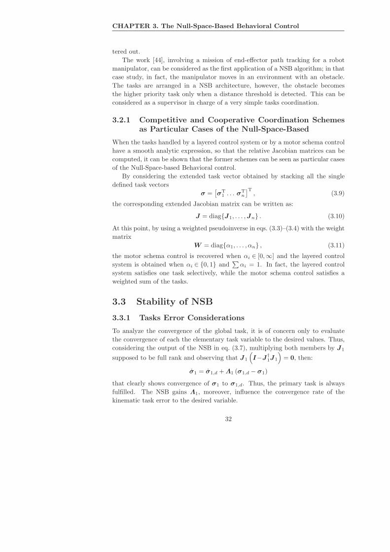
CHAPTER 3. The Null-Space-Based Behavioral Control
tered out.
The work [44], involving a mission of end-effector path tracking for a robot
manipulator, can be considered as the first application of a NSB algorithm; in that
case study, in fact, the manipulator moves in an environment with an obstacle.
The tasks are arranged in a NSB architecture, however, the obstacle becomes
the higher priority task only when a distance threshold is detected. This can be
considered as a supervisor in charge of a very simple tasks coordination.
3.2.1 Competitive and Cooperative Coordination Schemes
as Particular Cases of the Null-Space-Based
When the tasks handled by a layered control system or by a motor schema control
have a smooth analytic expression, so that the relative Jacobian matrices can be
computed, it can be shown that the former schemes can be seen as particular cases
of the Null-Space-based Behavioral control.
By considering the extended task vector obtained by stacking all the single
defined task vectors
σ =[σT
1 . . . σTn
]T, (3.9)
the corresponding extended Jacobian matrix can be written as:
J = diag{J1, . . . ,Jn} . (3.10)
At this point, by using a weighted pseudoinverse in eqs. (3.3)–(3.4) with the weight
matrix
W = diag{α1, . . . , αn} , (3.11)
the motor schema control is recovered when αi ∈ [0,∞] and the layered control
system is obtained when αi ∈ {0, 1} and∑αi = 1. In fact, the layered control
system satisfies one task selectively, while the motor schema control satisfies a
weighted sum of the tasks.
3.3 Stability of NSB
3.3.1 Tasks Error Considerations
To analyze the convergence of the global task, it is of concern only to evaluate
the convergence of each the elementary task variable to the desired values. Thus,
considering the output of the NSB in eq. (3.7), multiplying both members by J1
supposed to be full rank and observing that J1
(I−J
†1J1
)= 0, then:
σ1 = σ1,d + Λ1 (σ1,d − σ1)
that clearly shows convergence of σ1 to σ1,d. Thus, the primary task is always
fulfilled. The NSB gains Λ1, moreover, influence the convergence rate of the
kinematic task error to the desired variable.
32

3.3 Stability of NSB
3.3.2 Lower Priority Tasks
The lower priority tasks are fulfilled only if they do not conflict with the high-
ers [45]. The non-conflicting relationship can be evaluated by mathematical con-
siderations about range and null-spaces of the (pseudo-inverse) Jacobians of the
task functions. E.g., considering the secondary task and multiply both members
of eq. (3.7) by J2, then:
σ2 = J2J†1 (σ1,d + Λ1 (σ1,d − σ1)) + σ2,d + Λ2 (σ2,d − σ2)
It it worth noticing that non-conflicting relationship between primary and sec-
ondary tasks can be expressed by:
J2J†1 = O, (3.12)
i.e.,
R(J†2) ⊥ R(J†
1). (3.13)
In that case, the two tasks, re-projected onto the vehicles velocity space, are
orthogonal and they can be fulfilled simultaneously. In fact, it results:
σ2 = σ2,d + Λ2 (σ2,d − σ2)
This condition is implied by
R(J†2) ⊆ N (J1). (3.14)
When a third task is added, the stability analysis of the first two is unchanged
because of the successive projection onto the higher priority null space. Following
the reasoning done for the second task, moreover, it can be observed that the third
task is decoupled from the first two if
R(J†3) ⊆ [N (J1) ∩N (J2)] . (3.15)
3.3.3 How Many Tasks Simultaneously?
The strong geometrical meaning of the proposed approach allows to easily dis-
cuss about the number of tasks to handle simultaneously. Let’s suppose that the
primary task, of a generic dimension m1, is fulfilled by a n-Degrees-Of-Freedom
(DOFs) robotic system. The null space of its Jacobian is a space of dimensions
n − r1 (where r1 ≤ m1 is the rank of the Jacobian). Supposing the secondary
task (of dimension m2 and rank r2 ≤ m2) is not conflicting with the primary task
(meaning that the secondary task acts in the null space of the primary task), the
null space of their combination has dimension n− r1 − r2. Choosing the tasks in a
way they are not conflicting, it is useful to add tasks until∑ri = n. Thus, once
33

CHAPTER 3. The Null-Space-Based Behavioral Control
covered all the degrees of freedom of the system, it is useless to add successive
tasks of lower priority since they will be projected on to an empty space (thus
giving always a null contribution to the system velocity). In case of conflicting
tasks, it is not possible to do any generic assumption regarding the useful number
of tasks but, case by case, intersection among null spaces should be analyzed.
In case of a differential drive mobile robot, not considering the vehicle orienta-
tion, it is n = 2 and it is thus clear that, once the DOFs are fulfilled, it is useless
to add other tasks. However, in the case of a multi-robot systems made up of N
mobile robots, the DOFs are n = 2N and can be easily handled with a geometric
approach of this kind.
This is not evident for the cooperative approach, where the designer often adds
several tasks even after having fulfilled the system DOFs, or, on the other side,
does not have a clear view of the remaining DOFs to be exploited. In literature
it is easy to find several task merged even for a single 2-DOFs mobile robot. As
it will be noticed in the Subsection 3.4.1, this causes a corruption of all the tasks’
velocities, even the ones of higher priority.
3.4 Comparison with Competitive and Coopera-
tive Approaches
3.4.1 Task Velocity Composition Comparison
Let’s consider the very simple situation of a 2-DOFs mobile robot moving under
the effect of the two behaviors:
• Task #1: obstacle-avoidance
• Task #2: move-to-goal
being the first of higher priority than the second; the corresponding task outputs
are the velocity vectors v1 and v2 and the velocity command to the robot is the
velocity vector vd. In absence of obstacles, the obstacle-avoidance task outputs a
zero velocity and the robot moves according to the sole move-to-goal command,
i.e., vd ≡ v2. In a situation such as the one reported in Figure 3.5 the two single
task velocities are non null and a suitable velocity command to the robot must be
decided.
In the case of the layered control system the obstacle-avoidance behavior sub-
sumes the move-to-goal one and the resulting velocity command to the robot will
then be vd ≡ v1 (see Figure 3.6). In the case of the motor schema control the
outputs of the two tasks are weighted, summed and normalized as shown in Fig-
ure 3.7. Of course, the selection of the weights is a design choice and the proposed
example, thus, just shows one possibility.
34
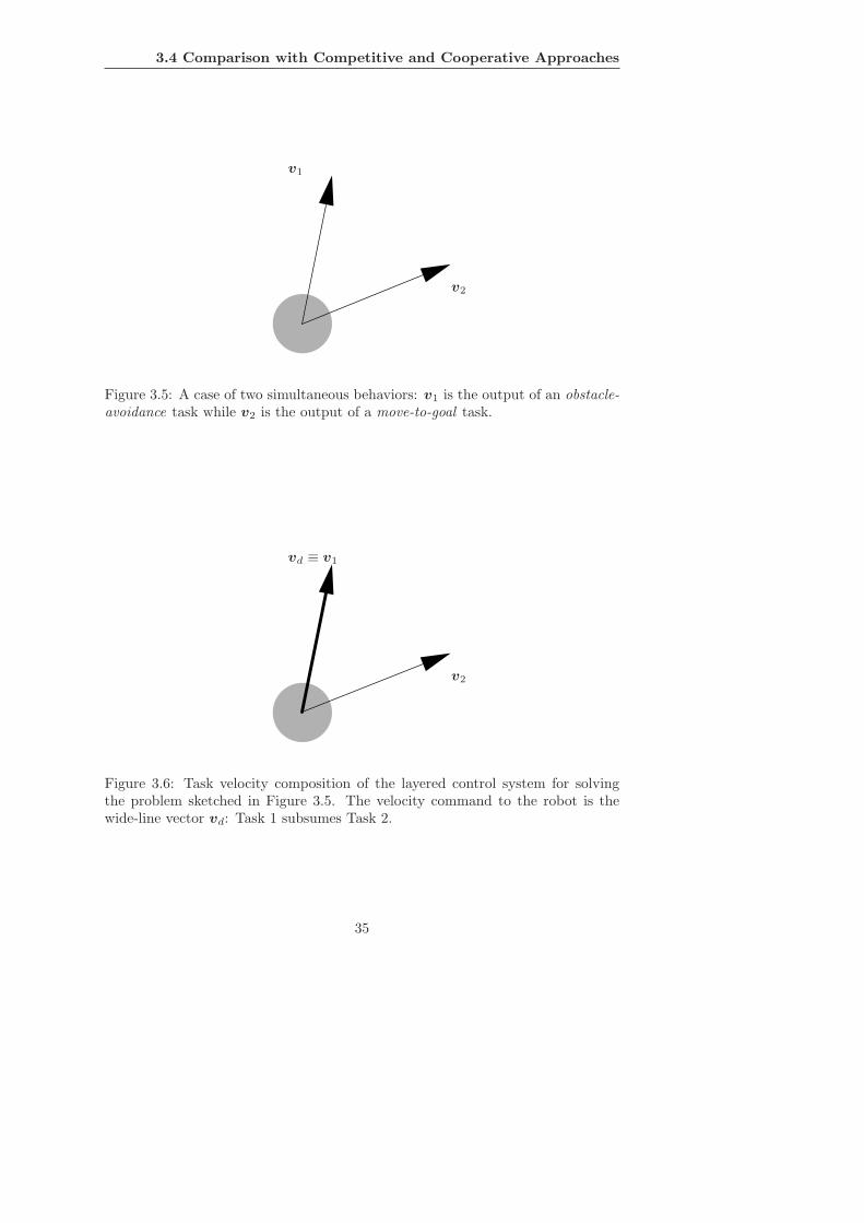
3.4 Comparison with Competitive and Cooperative Approaches
v1
v2
Figure 3.5: A case of two simultaneous behaviors: v1 is the output of an obstacle-avoidance task while v2 is the output of a move-to-goal task.
vd ≡ v1
v2
Figure 3.6: Task velocity composition of the layered control system for solvingthe problem sketched in Figure 3.5. The velocity command to the robot is thewide-line vector vd: Task 1 subsumes Task 2.
35

CHAPTER 3. The Null-Space-Based Behavioral Control
α1v1
α2v2
∑αivi
vd
Figure 3.7: Task velocity composition of the motor schema control for solving theproblem sketched in Figure 3.5. The velocity command to the robot is the wide-line vector vd: the weight of Task 1 is 1.2 while the weight of Task 2 is 0.4 andthe norm of the weighted sum is saturated.
It is worth noticing in this simple example how the weighted sum of the task
outputs may cause conflict among the behaviors. In fact, as can be seen in Fig-
ure 3.7, the lower-priority (α2 = 0.4) Task 2 velocity has a component along the
higher-priority (α1 =1.2) Task 1 velocity that modifies its magnitude. As a result,
the robot does not fulfill one single task, even the higher-priority one, but a linear
combination of the tasks. Of course, if fulfillment of one single task is desired,
the supervisor must set the corresponding weight to unity while deactivating all
the other tasks; in this case, except for the presence of the supervisor, the motor
schema control works similarly to a layered control system.
In the case of the Null-Space-based Behavioral approach, before being added to
the higher-priority Task 1 velocity, the lower-priority Task 2 velocity must be pro-
jected onto the the null space of the primary-task Jacobian matrix. If the primary
task is specified so as to ensure a minimum given distance from the obstacle (i.e.,
is expressed as a scalar function), its Jacobian has a monodimensional range space
aligned to the vehicle-obstacle direction and a monodimensional null space along
the orthogonal direction. Therefore, by projecting the secondary task velocity onto
the null space of J1, the component of v2 that would affect the vehicle-obstacle
distance is filtered out (see Figure 3.8); on the other hand, the other component
of v2 results in a slide-around-the-obstacle motion.
36

3.4 Comparison with Competitive and Cooperative Approaches
v1
v2
(I − J
†1J1
)v2
vd
Figure 3.8: Task velocity composition of the Null-Space-based Behavioral controlfor solving the problem sketched in Figure 3.5. The move-to-goal velocity is pro-jected onto the null space of the higher-priority obstacle-avoidance Jacobian. Theresulting motion is so that the vehicle slides around the obstacle.
3.4.2 Comparison in a Move-to-Goal Mission with an Uni-
cycle Robot
In this Section, a simulative and experimental comparison among the different
behavioral approaches is investigated in a move-to-goal mission involving a single
grounded mobile robot. In the proposed case, the move-to-goal overall mission is
decomposed in two elementary tasks, namely:
• Task #1: obstacle-avoidance;
• Task #2: move-to-goal.
a) Obstacle-avoidance
The obstacle-avoidance is the highest priority task because its achievement
is of crucial importance to preserve the integrity of the vehicle. In presence
of an obstacle in the advancing direction, its aim is to keep the robot on
a safe distance from the obstacle. Thus, its implementation elaborates as
output a velocity, in the robot-obstacle direction, that keep the robot to a
safe distance from the obstacle. Therefore, it is:
σ1 = ‖p − po‖ ∈ IR
σ1,d = d
J1 = rT ∈ IR1×2 ,
where po is the obstacle position and
r =p − po
‖p − po‖
37
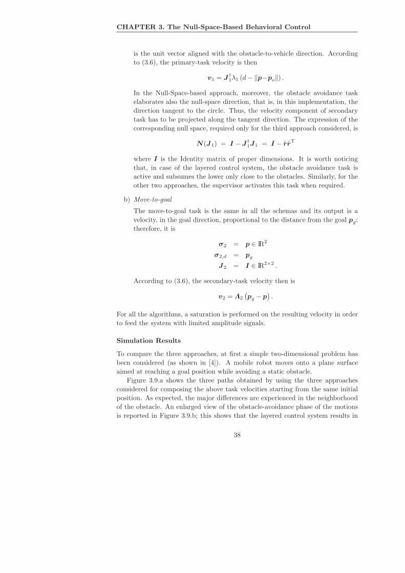
CHAPTER 3. The Null-Space-Based Behavioral Control
is the unit vector aligned with the obstacle-to-vehicle direction. According
to (3.6), the primary-task velocity is then
v1 = J†1λ1 (d− ‖p−po‖) .
In the Null-Space-based approach, moreover, the obstacle avoidance task
elaborates also the null-space direction, that is, in this implementation, the
direction tangent to the circle. Thus, the velocity component of secondary
task has to be projected along the tangent direction. The expression of the
corresponding null space, required only for the third approach considered, is
N(J1) = I − J†1J1 = I − rr
T
where I is the Identity matrix of proper dimensions. It is worth noticing
that, in case of the layered control system, the obstacle avoidance task is
active and subsumes the lower only close to the obstacles. Similarly, for the
other two approaches, the supervisor activates this task when required.
b) Move-to-goal
The move-to-goal task is the same in all the schemas and its output is a
velocity, in the goal direction, proportional to the distance from the goal pg;
therefore, it is
σ2 = p ∈ IR2
σ2,d = pg
J2 = I ∈ IR2×2 .
According to (3.6), the secondary-task velocity then is
v2 = Λ2
(pg − p
).
For all the algorithms, a saturation is performed on the resulting velocity in order
to feed the system with limited amplitude signals.
Simulation Results
To compare the three approaches, at first a simple two-dimensional problem has
been considered (as shown in [4]). A mobile robot moves onto a plane surface
aimed at reaching a goal position while avoiding a static obstacle.
Figure 3.9.a shows the three paths obtained by using the three approaches
considered for composing the above task velocities starting from the same initial
position. As expected, the major differences are experienced in the neighborhood
of the obstacle. An enlarged view of the obstacle-avoidance phase of the motions
is reported in Figure 3.9.b; this shows that the layered control system results in
38
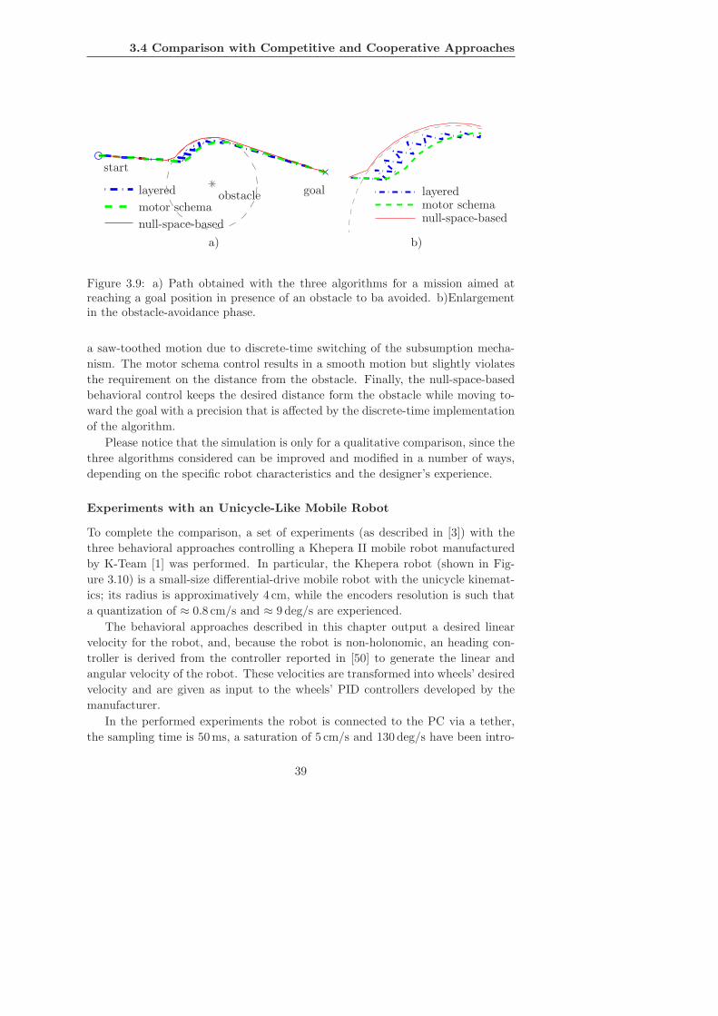
3.4 Comparison with Competitive and Cooperative Approaches
obstacle
start
goallayered
motor schema
null-space-based
layeredmotor schemanull-space-based
a) b)
Figure 3.9: a) Path obtained with the three algorithms for a mission aimed atreaching a goal position in presence of an obstacle to ba avoided. b)Enlargementin the obstacle-avoidance phase.
a saw-toothed motion due to discrete-time switching of the subsumption mecha-
nism. The motor schema control results in a smooth motion but slightly violates
the requirement on the distance from the obstacle. Finally, the null-space-based
behavioral control keeps the desired distance form the obstacle while moving to-
ward the goal with a precision that is affected by the discrete-time implementation
of the algorithm.
Please notice that the simulation is only for a qualitative comparison, since the
three algorithms considered can be improved and modified in a number of ways,
depending on the specific robot characteristics and the designer’s experience.
Experiments with an Unicycle-Like Mobile Robot
To complete the comparison, a set of experiments (as described in [3]) with the
three behavioral approaches controlling a Khepera II mobile robot manufactured
by K-Team [1] was performed. In particular, the Khepera robot (shown in Fig-
ure 3.10) is a small-size differential-drive mobile robot with the unicycle kinemat-
ics; its radius is approximatively 4 cm, while the encoders resolution is such that
a quantization of ≈ 0.8 cm/s and ≈ 9 deg/s are experienced.
The behavioral approaches described in this chapter output a desired linear
velocity for the robot, and, because the robot is non-holonomic, an heading con-
troller is derived from the controller reported in [50] to generate the linear and
angular velocity of the robot. These velocities are transformed into wheels’ desired
velocity and are given as input to the wheels’ PID controllers developed by the
manufacturer.
In the performed experiments the robot is connected to the PC via a tether,
the sampling time is 50 ms, a saturation of 5 cm/s and 130 deg/s have been intro-
39
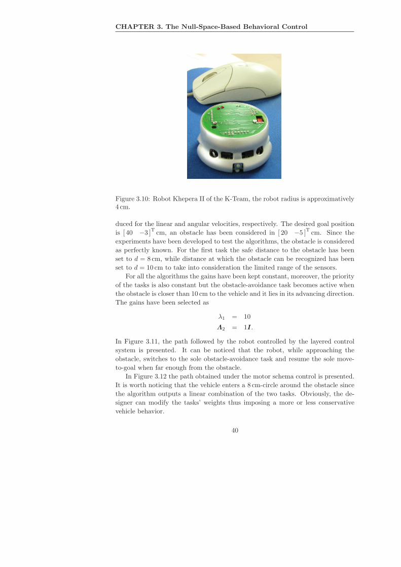
CHAPTER 3. The Null-Space-Based Behavioral Control
Figure 3.10: Robot Khepera II of the K-Team, the robot radius is approximatively4 cm.
duced for the linear and angular velocities, respectively. The desired goal position
is [ 40 −3 ]T
cm, an obstacle has been considered in [ 20 −5 ]T
cm. Since the
experiments have been developed to test the algorithms, the obstacle is considered
as perfectly known. For the first task the safe distance to the obstacle has been
set to d = 8 cm, while distance at which the obstacle can be recognized has been
set to d = 10 cm to take into consideration the limited range of the sensors.
For all the algorithms the gains have been kept constant, moreover, the priority
of the tasks is also constant but the obstacle-avoidance task becomes active when
the obstacle is closer than 10 cm to the vehicle and it lies in its advancing direction.
The gains have been selected as
λ1 = 10
Λ2 = 1I.
In Figure 3.11, the path followed by the robot controlled by the layered control
system is presented. It can be noticed that the robot, while approaching the
obstacle, switches to the sole obstacle-avoidance task and resume the sole move-
to-goal when far enough from the obstacle.
In Figure 3.12 the path obtained under the motor schema control is presented.
It is worth noticing that the vehicle enters a 8 cm-circle around the obstacle since
the algorithm outputs a linear combination of the two tasks. Obviously, the de-
signer can modify the tasks’ weights thus imposing a more or less conservative
vehicle behavior.
40

3.4 Comparison with Competitive and Cooperative Approaches
obstacle
start
goal
x [cm]
y[c
m]
t [s]
t [s]
v[c
m/s
]
ω[d
egre
e/s]
-10
-5
0
0
0
0
0
0
2
2
2
4
4
4
5
6
6
6
8
8
10
10
10
12
12
20 30 40
50
100
150
-50
-100
-150
Figure 3.11: Layered control system: a) Path followed for reaching a goal inpresence of obstacle. b)Odometric measure of linear velocity of the robot. c)Odometric measure of angular velocity of the robot.
41

CHAPTER 3. The Null-Space-Based Behavioral Control
obstacle
start
goal
x [cm]y
[cm
]
t [s]
t [s]
v[c
m/s
]
ω[d
egre
e/s]
-10
-5
0
0
0
0
0
0
2
2
2
4
4
4
6
6
6
8
8
10
10
10
12
12
20 30 40
50
100
150
-50
-100
-150
Figure 3.12: Motor schema: a) Path followed for reaching a goal in presenceof obstacle. b)Odometric measure of linear velocity of the robot. c) Odometricmeasure of angular velocity of the robot.
42
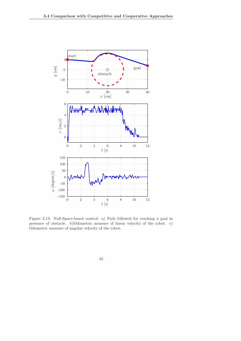
3.4 Comparison with Competitive and Cooperative Approaches
obstacle
start
goal
x [cm]
y[c
m]
t [s]
t [s]
v[c
m/s
]
ω[d
egre
e/s]
-10
-5
0
0
0
0
0
0
2
2
2
4
4
4
6
6
6
8
8
10
10
10
12
12
20 30 40
50
100
150
-50
-100
-150
Figure 3.13: Null-Space-based control: a) Path followed for reaching a goal inpresence of obstacle. b)Odometric measure of linear velocity of the robot. c)Odometric measure of angular velocity of the robot.
43

CHAPTER 3. The Null-Space-Based Behavioral Control
In Figure 3.13.a, the path followed with the Null-Space-based control is shown.
The geometric characteristic of this approach can be easily verified, during the
obstacle avoidance, in fact, the vehicle keeps the safe distance from the obstacle
exactly, thus fulfilling the higher priority task, and uses its null space in order
to try to fulfill the lower priority task. The overall motion is a clean sliding of
the vehicle around the safe circle. In Figures 3.13.b and 3.13.c the corresponding
measured values of the linear and angular velocities are shown.
3.5 NSB in a Kick-to-Goal Mission with a Unicy-
cle Robot
In this section, the mission of a soccer-playing mobile robot kicking a ball in a
goal referring to the NSB approach will be considered (see Figure 3.14).
Figure 3.14: Robot Khepera II of the K-Team with the rubber ball used in theexperiment.
As described in [5], the supervisor (see Figure 3.4) has been implemented re-
sorting to a Finite-State System. Notice that the specific technique used in order
to implement the supervisor is a designer’s choice and will not modify the NSB
architecture; in [12], for example, the supervisor has been designed resorting to
a fuzzy-based approach. For this specific mission the following states have been
considered:
⊲ prepare kick ;
⊲ execute kick ;
44

3.5 NSB in a Kick-to-Goal Mission with a Unicycle Robot
⊲ wait ;
⊲ hold rest position .
The actions are defined using simple rules based on information about sensors,
state and switching conditions. In particular:
• if the robot is in the prepare-kick state, it moves to a target position at a
proper distance from the ball along the ball-goal direction. While performing
this action, the robot has to avoid eventual obstacles (i.e. other robots or
the ball) present in the environment. When the robot reaches the target
position, the state switches to the execute-kick one;
• if the robot is in the execute-kick state, the robot moves at high velocity
toward the ball, aligning itself with the ball-goal direction; the consequent
impact, thus, represents the kick. Then, the state switches to the wait state;
• if the robot is in the wait state, the robot reduces its velocity and waits
to verify that the ball is moving correctly to the goal or that, due to an
imprecise impact or other disturbances, a second kick is required;
• the robot is in the hold-rest-position state if it recognizes to have correctly
put the ball in the goal; it then moves to the designed rest position.
For each state, the supervisor properly selects the elementary tasks that are to be
fulfilled and assigns their relative priority. Three tasks have been coded, namely
a) obstacle-avoidance;
b) move-to-goal;
c) execute-kick.
and the supervisor of the NSB architecture performs the task composition as
follows:
state primary secondaryprepare kick a bexecute kick c -wait a bhold rest position a b
Please notice that different states activate the same tasks but these can be
implemented with different gains; for instance, in the hold-rest-position state,
that is less critical than the prepare-kick state, lower positional gains might be
implemented to lower the energy consumption.
The tasks functions and the corresponding Jacobians are:
45

CHAPTER 3. The Null-Space-Based Behavioral Control
a) obstacle-avoidance. See section 3.4.2.a)
b) move-to-goal. See section 3.4.2.b)
c) execute-kick. In order to kick the ball, the vehicle needs to impact with it
in the ball-goal direction with an high velocity. Since this task needs two
degrees of freedom, its null space is the null set; this excludes the possibility
to fulfill a secondary task function, whose definition can be thus avoided.
Denoting as rg the unit vector aligned with the ball-to-kick direction and
with ∆θ the relative angle between rg and the vehicle-to-kick direction, it is
possible to define
vc = λc,1dg sign (∆θ) r⊥g + λc,2e
−∆θ2
α rg ,
where λc,1, λc,2 and α are control gains and dg is the distance of the vehicle
from the line connecting the ball and the goal.
In these experiments the mobile robot communicates with an host computer
via a radio link at 9600 bps. In case of perfect transmission the packets required for
the control can be transmitted in ≈70 ms. Since the radio-modem is equipped with
a correction/acknowledge algorithm, when a packet is lost it can be retransmitted
up to 10 times, thus resulting in a longer transmission time. In our experiments
the 95 % of the packets reached the vehicle in ≈70 ms but the remaining 5 % in a
larger time, thus resulting in a small phenomenon of random sampling.
The vehicle and the ball positions are measured by resorting to a vision-based
system working at a sampling time of 60 ms. The measurement error has an upper
bound of ≈0.5 cm and ≈1 deg.
According to the above considerations, the sampling time of the host PC is
selected as 100 ms. A saturation of 23 cm/s and 100 deg/s has been introduced for
the linear and angular velocities, respectively.
The desired goal position is [ 120 40 ]T
cm. Even in this experiment, the safe
distance to the obstacle for the Task a has been set to d=8 cm, while the distance
at which the obstacle can be recognized has been set to d=10 cm to simulate the
limited range of onboard sensors.
The gains have been selected as
λa = 1 Λb = I
λc,1 = 3 λc,2 = 30 α = 0.8 .
Several experiments have been run, in which the vehicle starts in the prepare-
kick state. When the vehicle is in position to kick, the state becomes the execute-
kick one. The supervisor is in charge of eventually switch back to the prepare-kick
state if the kick is not strong enough to reach the goal. When the ball is in the
46

3.5 NSB in a Kick-to-Goal Mission with a Unicycle Robot
Figure 3.15: Paths of different experiments as measured by the vision system: theball is sketched in the initial and final position, the vehicle path is shown in solidline and the ball path in dashed line.
goal or outside the field, the vehicle comes back to the rest position [ 80 30 ]T
cm.
In Figure 3.15 the paths of different experiments are shown; the ball is sketched
in the initial and final position, the vehicle path is shown in solid line and the ball
path in dashed line. The paths are as they have been measured by the vision
system. The robot case is not flat and the ball direction after the impact is
strongly influenced by the exact angle of impact with the robot. The ball’s surface,
moreover, is also not flat and in some experiments very unpredictable change of
direction is experienced.
In Figure 3.16, nine snapshots of one single run are reported. The supervisor
dynamically selects the active state and the corresponding tasks with their relative
priority. It is worth noticing that the vehicle has 2 degrees of freedom, it is thus
useless in our approach to arrange several tasks simultaneously, as instead is done
in a, e.g., cooperative behavioral approach.
In Figure 3.17, the repeatability of the experiment is analyzed. As it can be
observed, there is a polarization of the kicks due to the low level dynamic controller
error.
In Figure 3.18, the commanded linear and angular velocities to the low level
controller are reported. It can be shown that, despite the noise present in the
overall system, the NSB behavioral controller outputs smooth enough reference
values.
47

CHAPTER 3. The Null-Space-Based Behavioral Control
1. obstacle-avoidance1. obstacle-avoidance
1. obstacle-avoidance1. obstacle-avoidance
1. obstacle-avoidance1. obstacle-avoidance
2. move-to-goal2. move-to-goal
2. move-to-goal2. move-to-goal
2. move-to-goal2. move-to-goal1. execute-kick
1. execute-kick
1. execute-kick
t = 0 s t = 4 s t = 6 s
t = 7 s t = 8 s
t = 10 s
t = 10 s
t = 13 s t = 16 s
Figure 3.16: Active tasks during the multiple steps of a ”kicking a ball in goal”experiment. The vehicle needs two kicks to realize the goal.
48

3.5 NSB in a Kick-to-Goal Mission with a Unicycle Robot
Finally, it must be noticed that the mission is fulfilled most of the times. Few
failures have been experienced always due to major hardware breakdown of the
power system or of the communication channel.
Figure 3.17: Paths of different executions of the same experiment.
[s][s]
[deg
/s]
[cm
/s]
0
000 5
5
5 10
10
10 15
15
15
20
50
100
-50
-100
Figure 3.18: Linear and angular reference velocities for a one-kick experiments.The kick can be observed at t ≈ 6 seconds.
49

CHAPTER 3. The Null-Space-Based Behavioral Control
50

Chapter 4
NSB for Grounded
Multi-Robot Systems
The Null-Space-based Behavioral control presented in the previous chapter, using
the redundancy of a robotic system in the achievement of a single task to achieve
also the lower priority tasks, results particularly suitable for system with high
degrees of freedom. Following this consideration, in this chapter, the application
of the NSB to the control of grounded multi-robot systems will be presented.
For MRSs, in fact, the DOFs are nMRS = N nvehi (where nvehi are the DOFs
of the single vehicles and N is the number of vehicles that compose the team);
thus, increasing the dimension of the MRS, the redundancy of the system respect
to the achievement of a single task may increase and the NSB may permit to
perform several tasks simultaneously. Starting with the description of different
task functions realized for MRSs, in this chapter, the stability of some missions
will be discussed, some consideration on the implementation aspects to MRS will
be done, and, finally, the experimental results of several missions performed with
an experimental set-up made up of 7 Khepera II mobile robots will be shown.
4.1 Task Functions for Multi-Robot Systems
In Section 3.2, the NSB approach has been introduced in the general case of a
multi-robot system. In fact, the variable p of eq. 3.1 is the aggregate variable of
all the positions of the single robots:
p = [pT1 . . . pT
n ]T.
Thus, in the case of multi-robot systems, the task functions should be defined as
aggregate functions, i.e., functions of the global configuration of the system.
To control the shape of the team of robots, different aggregate task functions
have been defined, e.g., the barycenter, the variance, the shape of the formation,
51

CHAPTER 4. NSB for Grounded Multi-Robot Systems
etc. Managing these task functions and combining them with the proper priorities,
it is possible to control the team of robots and make it performing different kinds
of missions. In the following of this Section, different task functions for the generic
case of a team of robot moving in a 3D space will be presented in their mathe-
matical aspects, moreover, all these functions will be then applied to the 2D case
of surface vehicles. The definition in the 3D space is to due to the possibility to
use the NSB to control vehicle moving in the all space directions (i.e., underwater
or aerial robots).
4.1.1 Task Function for Platoon Barycenter
The barycenter of a platoon expresses the mean value of the vehicles positions. In
a 3-dimensional case the task function is expressed by:
σb = f b (p1, . . . , pn) =1
n
n∑
i=1
pi.
where pi = [xi yi zi ]T
is the position of the vehicle i.
By deriving the previous relation it holds:
σb =n∑
i=1
∂f b (p)
∂pi
vi = Jb (p) v
where the Jacobian matrix Jb ∈ IR3×3n is
Jb =1
n
. . .
1 0 00 1 00 0 1
. . .
.
whose pseudoinverse is simply given by
J†b =
...1 0 00 1 00 0 1
...
(4.1)
.
52

4.1 Task Functions for Multi-Robot Systems
The null space projector N (Jb) = I−J†bJb ∈ IR3n×3n is given by:
N (J b) =
1 − 1
n0 0 − 1
n0 0 − 1
n0 0
0 1 − 1
n0 0 − 1
n0 · · · 0 − 1
n0
0 0 1 − 1
n0 0 − 1
n0 0 − 1
n
− 1
n0 0 1 − 1
n0 0 − 1
n0 0
0 − 1
n0 0 1 − 1
n0 · · · 0 − 1
n0
0 0 − 1
n0 0 1 − 1
n0 0 − 1
n
...− 1
n0 0 − 1
n0 0 1 − 1
n0 0
0 − 1
n0 0 − 1
n0 · · · 0 1 − 1
n0
0 0 − 1
n0 0 − 1
n0 0 1 − 1
n
(4.2)
and it can be easily verified that its rank is 3(n − 1). One obvious conclusion
is that, with a 1-single robot platoon, the task of controlling its average position
saturates the available DOFs and the null space has null rank.
Following equation (3.4), the output of the barycenter task function is:
vb = J†b
(σb,d + Λbσb
), (4.3)
where the desired value of the task function represents the desired trajectory of
the barycenter.
4.1.2 Task Function for Platoon Mono-Dimensional Vari-
ance
Together with the platoon barycenter, it is of interest to consider the variance
of all the vehicles’ positions as a synthetic data on their spreading around the
barycenter. By controlling these two task variables it is possible to influence the
shape of the platoon.
The task function for platoon variance σv ∈ IR1 is defined as
σv =1
n
n∑
i=1
(pi − p)T(pi − p), (4.4)
whose (1 × 3n) Jacobian, defined for n > 1, is
Jv =2(n− 1)
n2[ . . . (pi − p)T . . . ] (4.5)
and whose (3n× 1) pseudoinverse is
J†v =
n2
2(n− 1)
...(pi − p)
(pi − p)T(pi − p)...
(4.6)
53

CHAPTER 4. NSB for Grounded Multi-Robot Systems
4.1.3 Task Function for Platoon 3D Variance
A different definition of the variance task function may consist in independently
considering the single components of the variance in the three dimensions of the
space. Individually controlling these values it is possible to make the platoon
reaching an ellipsoidal shape of the variance (vs. a spherical one for the mono-
dimensional case of Section 4.1.2).
The task function for platoon 3D variance σv ∈ IR3 is defined as
σv =1
n
n∑
i=1
(xi−x)2
(yi−y)2
(zi−z)2
, (4.7)
whose (3 × 3n) Jacobian is
Jv =2(n− 1)
n2
xi−x 0 0· · · 0 yi−y 0 · · ·
0 0 zi−z
(4.8)
and whose pseudoinverse is
J†v =
n2
2(n− 1)
...
xi−xn∑
j=1
(xj−x)20 0
0yi−y
n∑
j=1
(yj−y)20
0 0 zi−zn∑
j=1
(zj−z)2
...
. (4.9)
The Jacobian Jv associated with the platoon variance may loose full rank at
some system configuration, in this case, the use of some singularity-robust inverse
kinematics, e.g., based on a damped least-squares inverse of the Jacobian [131],
would provide a smooth reference trajectory.
The output of the barycenter task function is
vv = J†v
(σv,d + Λvσv
), (4.10)
where the desired value of the task function represents the desired components of
the ellipsoid of variance.
54
4.1 Task Functions for Multi-Robot Systems
4.1.4 Task Function for Rigid Formation
The rigid formation task moves the vehicles to a predefined formation relative to
the barycenter. The task function is defined as:
σf =
p1 − pb
...pn − pb
,
where pi are the coordinates of the vehicle i and pb = σb are the coordinates of
the barycenter. The corresponding Jacobian matrix Jf ∈ IR3n×3n is:
Jf =
A O O
O A O
O O A
, (4.11)
where
A =
1− 1n − 1
n . . . − 1n
− 1n 1− 1
n . . . − 1n
......
. . ....
− 1n − 1
n . . . 1− 1n
(4.12)
and O is a 3n× 3n null matrix.
Because the Jacobian matrix is singular, the pseudoinverse can not be calcu-
lated as JT(JJT
)−1
but as a matrix that verifies the following properties:
JJ†J = J†; J†JJ† = J
and with JJ† and J†J symmetric. Since Jf is symmetric and idempotent,
J†f = Jf .
The desired value σf,d of the task function describes the shape of the desired
formation; that is, once defined the formation, the elements of σf,d represent the
coordinates of each vehicle in the barycenter reference frame.
The output of the formation task function, in the case of fixed desired formation
(σf,d = 0), is:
vf = J†fΛf σf (4.13)
55
CHAPTER 4. NSB for Grounded Multi-Robot Systems
4.1.5 Task Function for Keeping a Platoon on the Surface
of a Sphere
The n-dimensional task function
σs =
...
1
2(pi − ci)
T(pi − ci)
...
(4.14)
can be used to keep each vehicle of the platoon at a given distance ri from a
point ci∈ IR3 by setting
σs,d =
...r2i /2
...
. (4.15)
The corresponding Jacobian is given by the (n×3n) matrix:
Js = block diag{(p1−c1)T, . . . , (pn−cn)T} (4.16)
whose pseudoinverse is the (3n×n) matrix:
J†s = block diag
{(p
1−c1)
(p1−c1)T(p
1−c1)
, . . . ,(p
n−cn)
(pn−cn)T(p
n−cn)
}. (4.17)
The above task function (4.14) can be used to keep the platoon on the surface
of a sphere by simply choosing the ci’s at the common value c, which represents
the center of the sphere, and setting all the ri’s at the same value r, which is the
radius of the sphere; namely
σs =
...
1
2(pi − c)T(pi − c)
...
(4.18)
σs,d =
...r2/2
...
. (4.19)
The corresponding expressions of the Jacobian and of its pseudoinverse are easily
obtained from eqs. (4.16) and (4.17), respectively.
56
4.1 Task Functions for Multi-Robot Systems
4.1.6 Task Function for Escorting a Target
In an escorting mission the platoon might be asked to keep the target at the
barycenter while the single vehicles lay at the same distance from the target and
minimize the intruding possibilities of an external agent. Dually, the same require-
ment concerns an entrapment mission.
With reference to the planar case, this requirement is satisfied by placing the
n vehicles at the vertices of a regular polygon of order n, the sides of which,
thus, define a sort of intrusion/escape window. A possible way to achieve this
formation is to keep the vehicles on a suitable circle through the above-defined task
function (4.18) while maximizing the mutual distance between adjacent vehicles.
The latter task can be achieved by properly assigning the perimeter of the polygon
inscribed in the circle; in fact, a regular polygon has the maximum perimeter
among all the polygons of the same order inscribed in a given circle.
Let’s define a n-dimensional vector k that collects the indexes to the vehicles
in their order along the circle. Thus, kj (i.e., the j-th coordinate of vector k) is the
index that identifies the vehicle at the j-th place along the circle —not necessarily
the j-th vehicle— and kj , kj+1 index two consecutive vehicles along the circle.
Obviously, any vehicle can be chosen as k1 and kn, k1 are consecutive.
The sought task function is thus given by a measurement of the perimeter,
such as
σp =1
2(pk1
−pkn)T(pk1
−pkn) +
1
2
n∑
j=2
(pkj−pkj−1
)T(pkj−pkj−1
) , (4.20)
whose Jacobian Jp ∈ IR1×2n is
Jp =[. . .
((pkj
−pkj−1)T+(pkj
−pkj+1)T
). . .
]. (4.21)
It is worth noticing that the vector k dynamically changes during the mission, i.e.,
no predefined position is imposed on the vehicles.
At this point, for a platoon of n vehicles that must entrap a target while
guaranteeing a given length l of the escape window, the radius of the circle in (4.19)
must be set to
r =l
2 cos(π
2− π
n
) (4.22)
and the desired value of the perimeter is simply
σp,d = n l . (4.23)
On the other hand, for a platoon of n vehicles that must entrap a target while
guaranteeing a given (safety) distance r of the vehicles from the target, the radius
57
CHAPTER 4. NSB for Grounded Multi-Robot Systems
of the circle in (4.19) is simply equal to r itself and the desired value of the
perimeter is
σp,d = 2n r cos(π
2− π
n
). (4.24)
4.1.7 Obstacle and Collision Avoidance
The obstacle avoidance task function is built individually for each vehicle, i.e., it
is not an aggregate task function. Each vehicle needs to avoid both environmental
obstacles and the other vehicles.
With reference to the generic surface vehicle in the team, in presence of an
obstacle in the advancing direction, the task function has to elaborate a driving
velocity, aligned to the vehicle-obstacle direction, that keeps the vehicle at a safe
distance d from the obstacle. Therefore, it is:
σo = ‖p − po‖σo,d = d
Jo = rT ,
where po is the obstacle position and
r =p − po
‖p − po‖
is the unit vector aligned with the obstacle-to-vehicle direction. According to the
above choice, eq. (3.6) simplifies to
vo = J†oλoσo = λo (d− ‖p − po‖) r. (4.25)
It is worth noting that, being
N (Jo) = I − rrT ,
the tasks of lower priority with respect to the obstacle avoidance are only allowed
to produce motion components tangent to the circle of radius d and centered in po
(also called safety area), so as to not interfere with the enforcement of the safe
distance d. Thus, a robot that is going to collide with a punctual obstacle does slide
on its safety area with an instantaneous velocity that depends on the projection
along the tangential direction of the velocities elaborated by the other tasks. If the
robot is going to frontally collide the obstacle (the velocity elaborated by the other
tasks is in the vehicle-obstacle direction), then the projection along the tangential
direction is null. This particular situation gives rise to a local minimum that
makes the robot stop. Nevertheless, the experimental experience evidenced that
the presence of measurement noise allows the vehicle to avoid the local minima;
this is, in fact, an unstable stationary point.
58
4.2 Stability
The obstacle avoidance function is developed for dot-like obstacles or obstacles
that may be conveniently rounded by a circle. In some cases, however, the obstacles
may be better represented by straight-lines or convex curves, in this case, po
represents the coordinates of the closest point of the obstacle to the vehicle at the
current time instant. In the experiments, both dot-like and linear obstacles will
be considered.
In the frequent case of multiple obstacles acting simultaneously (e.g., both an
obstacle in the environment and the other vehicles of the team) a priority among
their avoidance should be defined; a reasonable choice is to assign the currently
closest obstacle the highest priority. In critical situations the obstacle avoidance
function may give a null-velocity output; this causes delay to the mission or loss
of vehicles to the formation but increases safety of the approach.
4.2 Stability
Following the considerations of Section 3.3, in this section the stability of some of
the performed missions will be proved.
4.2.1 Stability for the Barycenter + Mono-Dimensional Vari-
ance
Let’s considering a mission composed by two tasks organized in the following
priority order:
1. Barycenter
2. Mono-Dimensional Variance
The stability of the mission is demonstrated showing that R(J†v) ⊆ N (Jb).
This relation does hold if the sole column of JTv can be expressed by a linear
combination of the columns of N (Jb).
The (3n× 1) transpose of the Jacobian for the Variance function is
JTv =
2(n− 1)
n2
(p1 − p)...
(pn − p)
. (4.26)
By defining as ni ∈ IR3n the i th column of the matrix N (Jb), it can be
observed that the span of the latter matrix is given by∑
i αini where the 3n
coefficients αi’s are the unknowns. By constructing a set of 3n linear equations
in 3n unknowns, however, one obtains again the matrix N (Jb) as the coefficients’
matrix. The set of linear equations to be solved in α ∈ IR3n is thus:
N (Jb)α = JTv . (4.27)
59
CHAPTER 4. NSB for Grounded Multi-Robot Systems
The problem seems to be numerically bad defined. However, it can be easily
observed that the last 3 equations are obtainable as linear combinations of the
previous equations. In particular, the sum of the equations gives zero. By simply
ignoring the last 3 equations the problem is well defined and this proves that the
R(JTv ) ⊆ N (Jb) that implies that R(J†
v) ⊆ N (Jb).
According to the former discussion the secondary task error decreases to the
null value when the primary is null and the pseudoinverse of the secondary is full
rank.
4.2.2 Stability for the Barycenter + 3D Variance
The primary task is the barycenter platoon position that, in view of the consid-
erations above, is convergent to the desired value. It can be observed by direct
calculations that
JvJ†b = O. (4.28)
On the other side, given
JTv =
2(n− 1)
n2
...xi−x 0 0
0 yi−y 00 0 zi−z
...
, (4.29)
and remembering that R(BT) ⊆ N (A) ⇒ R(B†) ⊥ R(A†), one possible
method to verify the stability is to check that the columns of JTv can be obtained
via a linear combination of the column of N (Jb). Let’s consider the first column
of JTv and define it as x of structure:
x = [x1 − x 0 0 x2 − x 0 0 · · · xn − x 0 0 ]T. (4.30)
Due to the structure of N (Jb) this should be given as a linear combination of
the sole elements of row i and column j with i ∈ {1, 4, · · · , 3(n − 1) + 1} and
j ∈ {1, 4, · · · , 3(n − 1) + 1}. It can be easily observed that the coefficients of the
linear combination of the selected columns of N (Jb) needed to obtain x are the
solution of a linear system of n equations and n unknowns where the coefficient
matrix is
1 − 1n
− 1n
− 1n
− 1n
1 − 1n
· · · − 1n
...− 1
n− 1
n1 − 1
n
(4.31)
that has null determinant. However, it is possible to make the same observations
done for the mono-dimensional case in order to verify that the last equation is
60

4.2 Stability
the sum of the previous ones. The problem, thus, admits a solution. This can be
extended for the remaining two columns of JTv and it is further possible to achieve
the same results as the average + mono-dimensional mission.
4.2.3 Stability for the Barycenter + Rigid Formation
The stability for the barycenter + rigid formation mission is straightforward by
observing that Jr ∈ IR3n×3n is equal to the null space projector of the barycenter
task function in eq. (4.2):
Jr = N (Jb). (4.32)
This implies, due to the matrix relationships above, that R(J†r) ⊆ N (Jb) without
need for further computations, or, equivalently, that JrJ†b = O.
4.2.4 Stability for the Barycenter + Platoon on a Sphere’s
Surface
Given the barycenter as primary task it is appropriate to modify the task function
to keep the platoon on the surface’s sphere in the n-dimensional task function
σs =
...
1
2(pi − p)T(pi − p)
...
(4.33)
whose Jacobian can be computed to be
Js =
(1 − 1
n
)(p
1− p)T − 1
n (p1− p)T − 1
n (p1− p)T
− 1n (p
2− p)T
(1 − 1
n
)(p
2− p)T . . . − 1
n (p2− p)T
...
− 1n (pn − p)T − 1
n (pn − p)T(1 − 1
n
)(pn − p)T
(4.34)
By repeating the same discussion made above, a solution for the set of linear
equations similar to eq. (4.27) is needed:
N (Jb)α = JTs (4.35)
in which N (Jb) ∈ IR3n×3n with rank 3(n−1). However, it possible to observe that
the equations of the linear systems are not linearly independent, in particular, it is
possible to verify that the last 3 equations are a linear combination, with unitary
weights, of the precedent equations. Removing them from the system makes it
possible to find the desired solution.
61
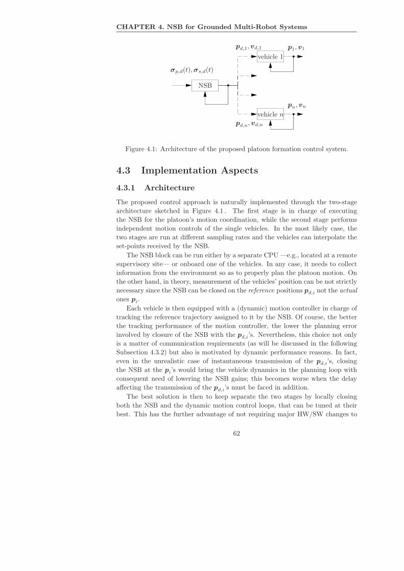
CHAPTER 4. NSB for Grounded Multi-Robot Systems
σp,d(t),σs,d(t)
NSB
pd,1,vd,1
vehicle 1
p1,v1
pd,n,vd,n
vehicle n
pn,vn
Figure 4.1: Architecture of the proposed platoon formation control system.
4.3 Implementation Aspects
4.3.1 Architecture
The proposed control approach is naturally implemented through the two-stage
architecture sketched in Figure 4.1 . The first stage is in charge of executing
the NSB for the platoon’s motion coordination, while the second stage performs
independent motion controls of the single vehicles. In the most likely case, the
two stages are run at different sampling rates and the vehicles can interpolate the
set-points received by the NSB.
The NSB block can be run either by a separate CPU —e.g., located at a remote
supervisory site— or onboard one of the vehicles. In any case, it needs to collect
information from the environment so as to properly plan the platoon motion. On
the other hand, in theory, measurement of the vehicles’ position can be not strictly
necessary since the NSB can be closed on the reference positions pd,i not the actual
ones pi.
Each vehicle is then equipped with a (dynamic) motion controller in charge of
tracking the reference trajectory assigned to it by the NSB. Of course, the better
the tracking performance of the motion controller, the lower the planning error
involved by closure of the NSB with the pd,i’s. Nevertheless, this choice not only
is a matter of communication requirements (as will be discussed in the following
Subsection 4.3.2) but also is motivated by dynamic performance reasons. In fact,
even in the unrealistic case of instantaneous transmission of the pd,i’s, closing
the NSB at the pi’s would bring the vehicle dynamics in the planning loop with
consequent need of lowering the NSB gains; this becomes worse when the delay
affecting the transmission of the pd,i’s must be faced in addition.
The best solution is then to keep separate the two stages by locally closing
both the NSB and the dynamic motion control loops, that can be tuned at their
best. This has the further advantage of not requiring major HW/SW changes to
62

4.3 Implementation Aspects
the individual controllers of the vehicles to become members of the platoon, that
in turn easily allows a vehicle to join or leave the team. To take into account the
unavoidable displacement of the actual vehicles’ position from the desired ones,
that may cause collisions, it is advisable that the task functions involving distances
from a vehicle are used with a tolerance threshold of the order of the maximum
tracking error of its motion controller.
4.3.2 Communication Requirements
According to Figure 4.1, the adopted architecture basically requires one-way com-
munication from the NSB algorithm to the vehicle controllers. Communication
among vehicles is not required because each vehicle needs to know only its own
state and its motion set-points coming from the NSB. With this approach, the
vehicles avoid mutual collision only through proper motion coordination at the
planning (NSB) level; nevertheless, to safely handle the uncertainty about the true
vehicle position inherent to this approach, a suitable tolerance must be ensured
when planning the relative distances.
The amount of data to be transmitted to each vehicle at each sampling time
is very low, since it only consists of a position and/or a velocity set-point. Never-
theless, the communication load grows with the cardinality of the platoon.
On the other hand, the NSB algorithm might benefit from collecting in real
time as much information about the environment as possible. This may come from
some global sensing device, e.g., a view from a camera that embraces the whole
scene, and/or from local sensory systems, e.g., a view from a camera mounted
onboard a vehicle. Some information may be absolute, such as a GPS reading,
some other may be relative, such as a distance measured by a sonar. In this
case, due to the very different possible scenarios, it is difficult to give a general
evaluation of the related communication requirement.
4.3.3 Computational Aspects
One important aspect of centralized schemes for the platoon control concerns the
growth of the computational load with the cardinality of the team. For instance
the computational complexity of graph-based algorithms grows exponentially with
the platoon’s number of members.
In the NSB case, the sole numerically demanding operation required is the
pseudoinversion of the Jacobians required in (3.6)–(3.7), which exhibits a polyno-
mial dependency on the matrix dimensions. It must be remarked, however, that
the chosen technique leads to Jacobians that only grow in the number of columns
with the number of vehicles of the platoon. This makes the pseudo inversion of
the Jacobians linearly dependent on the number of robots; in fact, the size of the
J iJTi square matrix to be inverted is invariantly equal to the dimension of the
63

CHAPTER 4. NSB for Grounded Multi-Robot Systems
i-th task. As usual, further advantage can be gained by taking into account the
specific numerical structure of the matrices to be pseudoinverted; as a matter of
fact, in most cases the task Jacobians are sparse matrices with several constant
1’s entries.
Last but not least, for most of the tasks considered in this thesis, the pseudoin-
version is computationally inexpensive since it can be symbolically derived. For
instance, for any mission in which the primary task is the platoon’s barycenter it
is clear that at least one pseudoinversion is not required.
4.4 Experiments with a Team of Khepera II
4.4.1 Experimental Setup
The NSB were tested while controlling a platoon of up to 7 Khepera II (see Fig-
ure 4.2) available at the LAI (Laboratorio di Automazione Industriale) of the
Universita degli Studi di Cassino. The Khepera II, manufactured by K-team [1],
are differential-drive mobile robots with a unicycle-like kinematics and with an
approximative dimension of 8 cm of diameter. Each Khepera has a Bluetooth tur-
ret that permits communication with the other robots or with external Bluetooth
devices. In the proposed set-up, each robot communicates with a remote Linux-
based PC, where a Bluetooth Dongle, building Virtual Serial Ports, allows the
communication with up to 7 robots (see Figure 4.3). The remote Linux-based PC
is aimed at implementing the NSB approach referring to a centralized structure.
Figure 4.2: Team of Khepera II mobile robots with the Bluetooth communicationmodules available at the LAI (Laboratorio di Automazione Industriale) of theUniversita degli Studi di Cassino.
Since the performed experiments focus on formation control, the vehicles po-
sitions are measured resorting to a vision-based system, made up of two high
64

4.4 Experiments with a Team of Khepera II
resolution color cameras and two frame-grabber Matrox Metor II, running on a
Windows-based PC. In particular, the upper turrets of each robot have a set
of colored LEDs (see Figure 4.4) that are used to detect positions, orientations
and identification numbers of each robot. The position measurements are per-
formed at a sampling time of 100 ms while the estimation error has an upper
bound of ≈ 0.5 cm and ≈ 1 deg. Moreover, the vision system permits to identify
static obstacles (e.g., the linear obstacles in Figure 4.3) or dynamic obstacles (i.e.,
a tennis ball) eventually present in the environment. The measurement are sent
over the LAN to the Linux-based PC using the UDP/IP protocol.
Figure 4.3: Experimental set-up available at the LAI (Laboratorio di AutomazioneIndustriale) of the Universita degli Studi di Cassino.
Following the approach described in the previous Sections, the NSB elaborates
the desired linear velocity for each robot of the team. Because the Kheperas are
unicycle-like robot (and not omnidirectional), an heading controller has been de-
rived from the controller reported in [95] to obtain wheels’ desired velocities (see
Figure 4.1). Thus, the remote Linux-based PC sends to each vehicle (through the
Bluetooth module) the wheels’ desired velocities with a sampling time of 120 ms.
The wheels’ controller (on board of each robot) is a PID developed by the manu-
facturer. A saturation of 40 cm/s and 180 deg/s has been introduced for the linear
and angular velocities, respectively. Moreover, the encoders resolution is such that
a quantization of ≈ 0.8 cm/s and ≈ 9 deg/s are experienced.
65
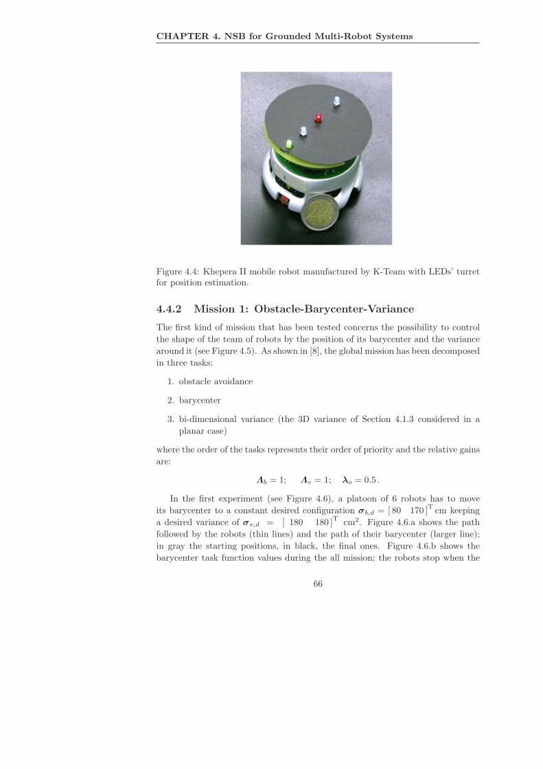
CHAPTER 4. NSB for Grounded Multi-Robot Systems
Figure 4.4: Khepera II mobile robot manufactured by K-Team with LEDs’ turretfor position estimation.
4.4.2 Mission 1: Obstacle-Barycenter-Variance
The first kind of mission that has been tested concerns the possibility to control
the shape of the team of robots by the position of its barycenter and the variance
around it (see Figure 4.5). As shown in [8], the global mission has been decomposed
in three tasks:
1. obstacle avoidance
2. barycenter
3. bi-dimensional variance (the 3D variance of Section 4.1.3 considered in a
planar case)
where the order of the tasks represents their order of priority and the relative gains
are:
Λb = 1; Λv = 1; λo = 0.5 .
In the first experiment (see Figure 4.6), a platoon of 6 robots has to move
its barycenter to a constant desired configuration σb,d = [ 80 170 ]T
cm keeping
a desired variance of σv,d = [ 180 180 ]T
cm2. Figure 4.6.a shows the path
followed by the robots (thin lines) and the path of their barycenter (larger line);
in gray the starting positions, in black, the final ones. Figure 4.6.b shows the
barycenter task function values during the all mission; the robots stop when the
66

4.4 Experiments with a Team of Khepera II
Figure 4.5: Initial and final configuration of the Barycenter-Variance task function.The red circle represents the desired barycenter position and variance, while theblue circle represents the measured values.
distance between the barycenter position and its desired position is lower then a
threshold value. Figure 4.6.c shows the variance values respect to the barycenter
along the axis x and y.
In the second experiment a platoon of 7 robots has to move its barycenter to
a constant desired configuration σb,d = [ 80 170 ]T
cm dynamically keeping three
different values of variance of σv,d = [ 300 300 ]T − [ 0 0 ]
T − [ 500 500 ]T
cm2.
Figure 4.7.a shows several steps of the mission execution, while Figures 4.7.b
and 4.7.c show respectively the barycenter task function values and the vari-
ance values along the axis x and y during the all mission. It is worth noticing
that the variance value relates to the density of the robots in the team, thus, a
small variance value makes the robot stay all close to the barycenter, an high
value make the robot spread in the environment. Please notice that the value
σv,d = [ 0 0 ]T
cm2 can not be reached because the obstacle avoidance task func-
tion, that is the highest priority task, does not allow the vehicles to have a relative
distance lower than 12 cm. The video of the relative experiment can be found in
the cd attached to this thesis (file: f varianza.wmv) or at the Author’s webpage
at: http://webuser.unicas.it/arrichiello
4.4.3 Mission 2: Obstacle-Barycenter-Rigid Formation
In the second mission, the robots have to reach and keep a rigid formation around
the barycenter (see Figure 4.8). Different conditions of the environment have been
considered, i.e., in the first experiment the robots have at first to reach a linear
formation in open space and then to invert their relative positions in the formation;
in the second experiment the same mission have to be performed in presence of
two linear static obstacles; in the last experiment the robots have to keep a static
67

CHAPTER 4. NSB for Grounded Multi-Robot Systems
0
50
50
100
100
150
150
200
200
x [cm]
y[c
m]
a)
[s]
00 10 20 30
50
100
150
[cm
]
[s]00 10 20 30
200
400
600
800
1000
1200[c
m2]
b) c)
Figure 4.6: First Barycenter-Variance experiment. a) Paths followed by the robotsduring the mission. b)Average task function: desired values of σb,d (dashed lines)and real values of σb (solid lines). c)Variance task function: desired values of σv,d
(dashed lines) and real values of σv (solid lines).
68

4.4 Experiments with a Team of Khepera II
t = 0 t = 14 t = 28 t = 42
t = 55 t = 68 t = 82 t = 95
a)
[s]
00
20
20
40
40
60
60
80
100
120
140
160
180
[cm
]
[s]
00 20 40 60
200
400
600
800
1000
[cm
2]
b) c)
Figure 4.7: Second Barycenter-Variance experiment. a) Snapshots of the exper-iment. b)Average task function: desired values of σb,d (dashed lines) and realvalues of σb (solid lines). c)Variance task function: desired values of σv,d (dashedlines) and real values of σv (solid lines).
69
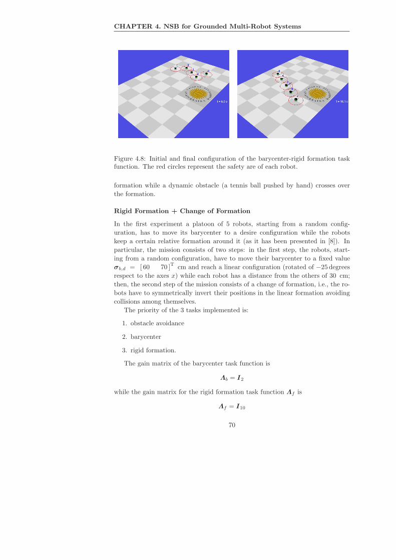
CHAPTER 4. NSB for Grounded Multi-Robot Systems
Figure 4.8: Initial and final configuration of the barycenter-rigid formation taskfunction. The red circles represent the safety are of each robot.
formation while a dynamic obstacle (a tennis ball pushed by hand) crosses over
the formation.
Rigid Formation + Change of Formation
In the first experiment a platoon of 5 robots, starting from a random config-
uration, has to move its barycenter to a desire configuration while the robots
keep a certain relative formation around it (as it has been presented in [8]). In
particular, the mission consists of two steps: in the first step, the robots, start-
ing from a random configuration, have to move their barycenter to a fixed value
σb,d = [ 60 70 ]T
cm and reach a linear configuration (rotated of −25 degrees
respect to the axes x) while each robot has a distance from the others of 30 cm;
then, the second step of the mission consists of a change of formation, i.e., the ro-
bots have to symmetrically invert their positions in the linear formation avoiding
collisions among themselves.
The priority of the 3 tasks implemented is:
1. obstacle avoidance
2. barycenter
3. rigid formation.
The gain matrix of the barycenter task function is
Λb = I2
while the gain matrix for the rigid formation task function Λf is
Λf = I10
70

4.4 Experiments with a Team of Khepera II
1
1
2
2
3
3
4
4
5
5
t = 0 t = 8 t = 16 t = 24
t = 50 t = 65 t = 80 t = 100
a)
[s]
00
20
40
50
60
80
100
100
120
140
160
180
[cm
]
[s]
00
20
40
50
60
80
100
100
120
140
[cm
]
b) c)
Figure 4.9: Rigid Formation + Change of Formation experiment. a) Snapshotsof the experiment. b)Average task function: desired values of σb,d (dashed lines)and real values of σb (solid lines). c)Rigid formation task function errors: normsof the error components of σf for each vehicle.
71
CHAPTER 4. NSB for Grounded Multi-Robot Systems
and the gain λo of the obstacle avoidance task function is
λo = 0.5
while σo,d is equal to 16 cm.
Figure 4.9 shows that the platoon does accomplish the mission avoiding the
collisions. In particular, Figure 4.9.a shows several steps of the mission execution
including desired values of the obstacle avoidance task functions. The robots
start from a random configuration and reach the first configuration in t ≈ 20 s do
avoiding collisions among themselves. At t = 50 s a new step input is commanded
to the platoon by requiring a change in the robots’ configuration while keeping the
same desired barycenter. Please notice that a quite severe command is given since
all the robots tend to cluster close to the barycenter in order to reach their new
positions in the formation. However, as can be see in Figure 4.9.b and Figure 4.9.c,
the robot correctly reach the new formation avoiding collisions (primary task)
and keeping low the barycenter error (second priority task) also in the transient
part. The algorithm, moreover, works often close to the local minima that might
arise with local obstacle avoidance algorithms. The irregularity of the trajectories
performed by the robots is due both to the obstacle avoidance task function (that
is activated only in when the distance between robots is lower than a threshold
value) and to the non-holonomy of the vehicles.
The video of the relative experiment can be found in the cd attached to this
thesis (file: f linear formation.wmv) or at the Author’s webpage at:
http://webuser.unicas.it/arrichiello
Rigid Formation + Linear Static Obstacles
In the second experiment (see Figure 4.10 and Figure 4.11), a platoon of 5 Khep-
era II have to perform the same mission of the previous case but in presence of
two linear static obstacles (as shown in [6]). Also this mission consists of two steps
(reaching the formation and switching the relative positions of the robots) but
in this case the first step takes longer than in the open space because one of the
robots (robot 5 of Figure 4.11.b) has to avoid the static obstacles switching on
their safety areas.
Figure 4.10 shows several steps of the mission execution including desired values
of the obstacle avoidance task functions, while Figure 4.11.b shows the paths
of the robots during the whole execution of the experiment. The robots start
from a random configuration (gray positions of Figure 4.11.b) and reach the first
configuration in t ≈ 20 s do avoiding collisions among themselves and with the
static obstacles. At t = 50 s a new step input is commanded to the platoon by
requiring a change in the robots’ configuration while keeping the same desired
barycenter.
72
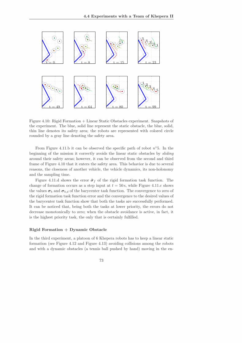
4.4 Experiments with a Team of Khepera II
1
1
2
2
3
3
4
4
5
5
t = 0 t = 8 t = 15 t = 23
t = 49 t = 64 t = 80 t = 99
Figure 4.10: Rigid Formation + Linear Static Obstacles experiment. Snapshots ofthe experiment. The blue, solid line represent the static obstacle, the blue, solid,thin line denotes its safety area; the robots are represented with colored circlerounded by a gray line denoting the safety area.
From Figure 4.11.b it can be observed the specific path of robot n◦5. In the
beginning of the mission it correctly avoids the linear static obstacles by sliding
around their safety areas; however, it can be observed from the second and third
frame of Figure 4.10 that it enters the safety area. This behavior is due to several
reasons, the closeness of another vehicle, the vehicle dynamics, its non-holonomy
and the sampling time.
Figure 4.11.d shows the error σf of the rigid formation task function. The
change of formation occurs as a step input at t = 50 s, while Figure 4.11.c shows
the values σb and σb,d of the barycenter task function. The convergence to zero of
the rigid formation task function error and the convergence to the desired values of
the barycenter task function show that both the tasks are successfully performed.
It can be noticed that, being both the tasks at lower priority, the errors do not
decrease monotonically to zero; when the obstacle avoidance is active, in fact, it
is the highest priority task, the only that is certainly fulfilled.
Rigid Formation + Dynamic Obstacle
In the third experiment, a platoon of 6 Khepera robots has to keep a linear static
formation (see Figure 4.12 and Figure 4.13) avoiding collisions among the robots
and with a dynamic obstacles (a tennis ball pushed by hand) moving in the en-
73

CHAPTER 4. NSB for Grounded Multi-Robot Systems
11
2 2
3
3
4
4
5
5
00
50
50
100
100
150
150
200
x [cm]
y[c
m]
a) b)
[s]
00
20
20
40
40
60
60
80
80
100
120
140
160
180
[cm
]
[s]
00
20
20
40
40
60
60
80
80
100
120
140
[cm
]
c) d)
Figure 4.11: a) Rigid Formation + Linear Static Obstacles experiment. b) Pathsfollowed by the Khepera II robots during the experimental mission. Gray, initialpositions; black, final positions. c)Average task function: desired values of σb,d
(dashed lines) and real values of σb (solid lines). d)Rigid formation task functionerrors: norms of the error components of σf for each vehicle.
74

4.4 Experiments with a Team of Khepera II
vironment. In particular, the desired position of the barycenter of the platoon is
σb,d = [ 75 90 ]T
cm, the linear formation is rotated of 65 degrees respect to the
axes x and the robots have to keep a distance of 30 cm one from the others.
0
0
0
0
0
0
0
0
0
0
0
0
0
0
0
0
50
50
50
50
50
50
50
50
50
50
50
50
50
50
50
50
100
100
100
100
100
100
100
100
100
100
100
100
100
100
100
100
150
150
150
150
150
150
150
150
150
150
150
150
150
150
150
150
-50-50-50-50
-50-50-50-50 t = 0 t = 2 t = 5 t = 7
t = 10 t = 12 t = 15 t = 17
Figure 4.12: Rigid Formation + Dynamic Obstacle. Several steps of the linearformation mission while a tennis ball is passing through the formation.
The priority of the 3 tasks implemented is:
1. obstacle avoidance
2. barycenter
3. rigid linear formation.
The gain matrix of the barycenter task function is
Λb = I2
while the gain matrix for the rigid formation task function Λf is
Λf = 2 ∗ I12.
The gain λo of the obstacle avoidance task function is
λo = 1
75
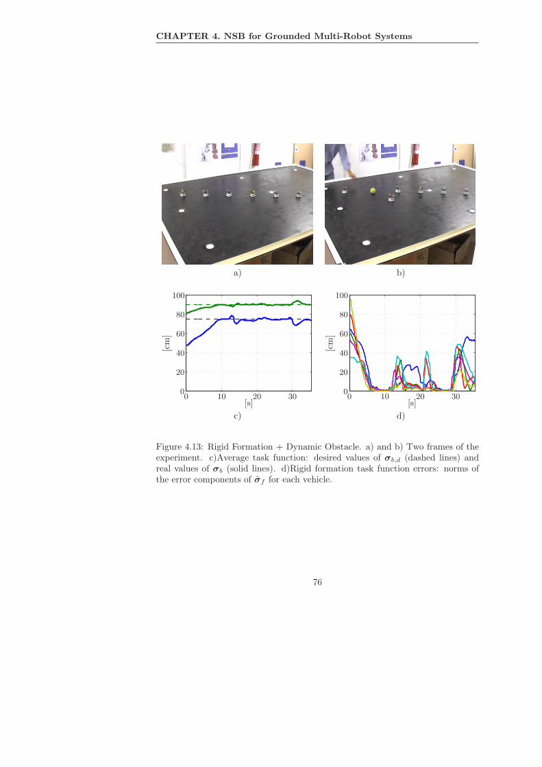
CHAPTER 4. NSB for Grounded Multi-Robot Systems
a) b)
[s]
00 10
20
20 30
40
60
80
100
[cm
]
[s]
00 10
20
20 30
40
60
80
100
[cm
]
c) d)
Figure 4.13: Rigid Formation + Dynamic Obstacle. a) and b) Two frames of theexperiment. c)Average task function: desired values of σb,d (dashed lines) andreal values of σb (solid lines). d)Rigid formation task function errors: norms ofthe error components of σf for each vehicle.
76
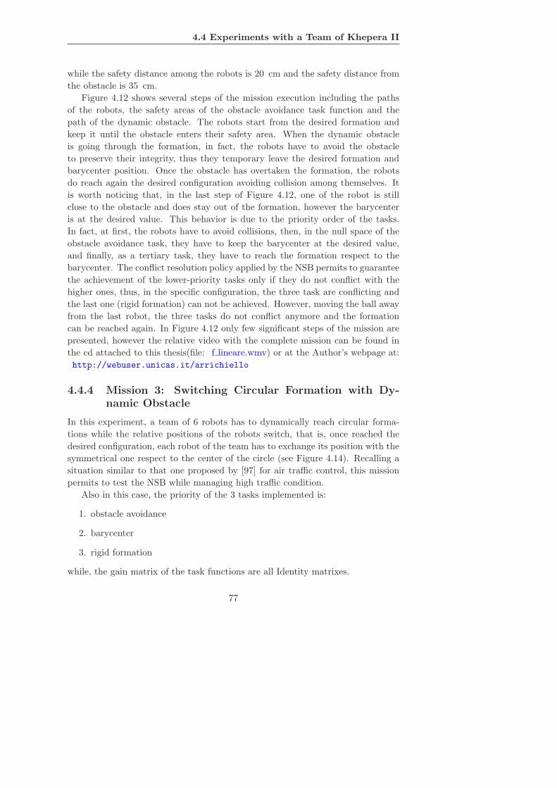
4.4 Experiments with a Team of Khepera II
while the safety distance among the robots is 20 cm and the safety distance from
the obstacle is 35 cm.
Figure 4.12 shows several steps of the mission execution including the paths
of the robots, the safety areas of the obstacle avoidance task function and the
path of the dynamic obstacle. The robots start from the desired formation and
keep it until the obstacle enters their safety area. When the dynamic obstacle
is going through the formation, in fact, the robots have to avoid the obstacle
to preserve their integrity, thus they temporary leave the desired formation and
barycenter position. Once the obstacle has overtaken the formation, the robots
do reach again the desired configuration avoiding collision among themselves. It
is worth noticing that, in the last step of Figure 4.12, one of the robot is still
close to the obstacle and does stay out of the formation, however the barycenter
is at the desired value. This behavior is due to the priority order of the tasks.
In fact, at first, the robots have to avoid collisions, then, in the null space of the
obstacle avoidance task, they have to keep the barycenter at the desired value,
and finally, as a tertiary task, they have to reach the formation respect to the
barycenter. The conflict resolution policy applied by the NSB permits to guarantee
the achievement of the lower-priority tasks only if they do not conflict with the
higher ones, thus, in the specific configuration, the three task are conflicting and
the last one (rigid formation) can not be achieved. However, moving the ball away
from the last robot, the three tasks do not conflict anymore and the formation
can be reached again. In Figure 4.12 only few significant steps of the mission are
presented, however the relative video with the complete mission can be found in
the cd attached to this thesis(file: f lineare.wmv) or at the Author’s webpage at:
http://webuser.unicas.it/arrichiello
4.4.4 Mission 3: Switching Circular Formation with Dy-
namic Obstacle
In this experiment, a team of 6 robots has to dynamically reach circular forma-
tions while the relative positions of the robots switch, that is, once reached the
desired configuration, each robot of the team has to exchange its position with the
symmetrical one respect to the center of the circle (see Figure 4.14). Recalling a
situation similar to that one proposed by [97] for air traffic control, this mission
permits to test the NSB while managing high traffic condition.
Also in this case, the priority of the 3 tasks implemented is:
1. obstacle avoidance
2. barycenter
3. rigid formation
while, the gain matrix of the task functions are all Identity matrixes.
77

CHAPTER 4. NSB for Grounded Multi-Robot Systems
Figure 4.14: Circular Switching Formation.
Figure 4.15.a shows several steps of the performed mission. Starting from a
linear configuration, the robots reach the circular formation in less the 20 s. Then,
once the error of the rigid formation task function has gone under a threshold
value, the robots have to change their relative configuration. In particular, each
robot has to exchange its position with its symmetrical respect to the center of
the circle (as can be noticed observing colors and numbers of the robots in the
steps 4, 8 and 12 of Figure 4.15.a). During the change of formation, all the robots
converge toward the center of the circle increasing the risk of collisions and of the
incurring of singular configurations. To significantly stress the algorithm, as shown
by the last four steps of Figure 4.15.a, a tennis ball pass through the circle while
the robot are changing the formation. Also in this case the change is correctly
achieved avoiding collision among the robots and with the obstacle. Thus, the
correct achievement of the mission allows to consider the approach robust to high
traffic condition and to conflict resolution.
Figures 4.15.b and 4.15.c show respectively the errors of the barycenter task
function and of the rigid formation task function. It is worth noticing that the
barycenter error is small during the all mission. However, it is not null because of
the nonholonomy of the robots and of the eventual obstacle. In an ideal case of
omnidirectional robots and ignoring the collision avoidance, the robot should keep
the barycenter in a constant position performing all the motions for changing the
configuration in the null space of the barycenter task. Figure 4.15.d shows that the
changes of formations are given as step functions and are correctly achieved also
in presence of obstacles. In particular, it is possible noticing that the third change
of formation takes longer and is more irregular than the previous ones because of
78
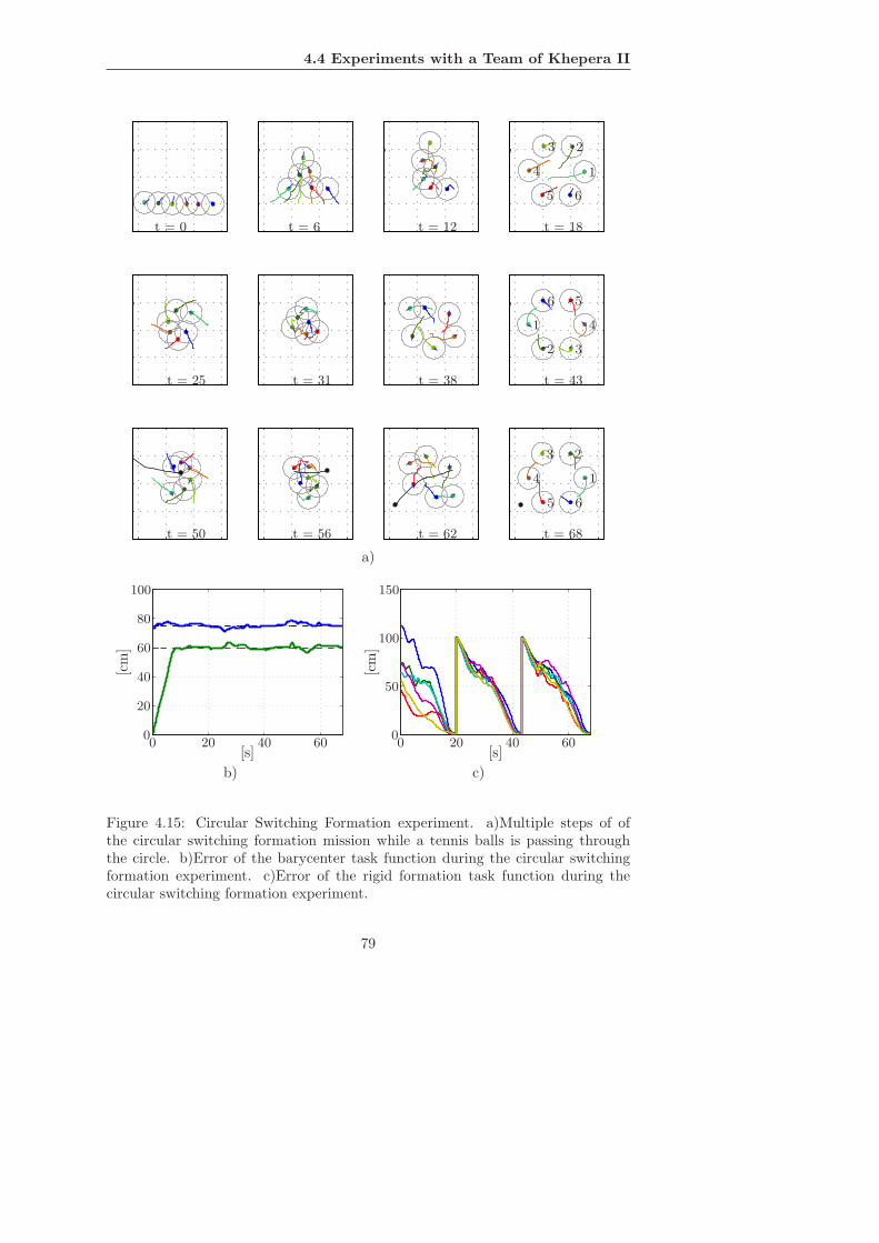
4.4 Experiments with a Team of Khepera II
1
1
1
2
2
2
3
3
3
4
4
4
5
5
5
6
6
6
t = 0 t = 6 t = 12 t = 18
t = 25 t = 31 t = 38 t = 43
t = 50 t = 56 t = 62 t = 68
a)
[s]00
20
20
40
40
60
60
80
100
[cm
]
[s]00 20 40
50
60
100
150
[cm
]
b) c)
Figure 4.15: Circular Switching Formation experiment. a)Multiple steps of ofthe circular switching formation mission while a tennis balls is passing throughthe circle. b)Error of the barycenter task function during the circular switchingformation experiment. c)Error of the rigid formation task function during thecircular switching formation experiment.
79

CHAPTER 4. NSB for Grounded Multi-Robot Systems
the ball is passing through the circle. The video of the relative experiment can be
found in the cd attached to this thesis (file: f circolare.wmv) or at the Author’s
webpage at: http://webuser.unicas.it/arrichiello
4.4.5 Mission 4: Escorting Mission
Another case studies is the escorting mission (see Figure 4.16): a tennis-ball is
the target to be entrapped by 6 Khepera II mobile robots. The vehicles should
guarantee an escaping window of 40 cm while the safety distance imposed to the
vehicles is 20 cm. The desired radius of the surrounding circle is modified accord-
ingly to the number of robots, i.e., it is modified during the experiment to take
into account loss of one or more vehicles.
Figure 4.16: Escorting mission.
At t ≈ 13 s one robot is moved away from the arena to simulate a failure, the
robot is put back in the arena at t ≈ 17 s, moreover, at t ≈ 23 s and t ≈ 28 s
the target is pushed twice to impose to the robots a reconfiguration. The relative
video of the experiment with the complete mission can be found in the cd attached
to this thesis (file: f scorta.mpg) or at the Author’s webpage at:
http://webuser.unicas.it/arrichiello
Figure 4.17 reports a label for the Figures 4.18 to 4.20 that show several snap-
shots of the mission. For the robots and the target, the paths of the last 3 s are
also reported with thin lines.
In Figure 4.18 the first 11 s of the experiment are reported. The target is
still and the vehicles are required to surround it. It can be observed that the
obstacle avoidance task is always the primary task and the vehicles avoid hitting
themselves during the movement, moreover, no predefined position is assigned
around the target. An hexagon-like configuration is the natural structure of the
80

4.4 Experiments with a Team of Khepera II
formation since the regular polygon guarantees the minimum distance between
adjacent points on a given circle.
target
robot
failed robot
Figure 4.17: Label of the following figures, the thin line represents the last 3-seconds path.
In Figure 4.19 the second group of snapshots are given, from t ≈ 12 s to t ≈ 23 s.
A fault is caused at t ≈ 13 s by moving away a robot by hand and further obscuring
it to the camera, after the reconfiguration is successfully achieved, the robot is put
again in the arena at t ≈ 17 s. The algorithm recognizes the absence of a robot
as a major fault, i.e., the vehicle is lost. The top plot represents the moment in
which one of the robot is moved away, the remaining vehicles are not anymore
minimizing the escape space of the target and need to reconfigure to achieve the
last-priority task, this can be seen in the second and third plots from the top of
Figure 4.19; from the geometrical point of view it can be observed that this is
achieved by positioning the vehicles from the edged of a 6-sides regular polygon
to a 5-sides regular one (third plot from the top) and modifying the desired radius
accordingly. Moreover, the vehicle is put back in the arena (fourth plot from the
top) and the formation is rearranged again after this occurrence. Notice that,
since the relative position is not predefined, the vehicle is positioning itself in the
circle with a different order (bottom plot).
To appreciate that the algorithm is working in real-time, the target is pushed
twice and the vehicles reconfigure such that the escort mission is still accomplished.
This can be appreciated in Figure 4.20 where the last ≈ 20 s of the mission are
reported. Moreover, it can also be observed that, after motion of the target, the
vehicles reconfigure themselves with a different relative position with respect to
the first steady-state condition. Also, from the bottom plot of the Figure it can
be observed a fuzzy path of the vehicles, one of the vehicles, in fact, experienced
a short not-recognized communication failure and the remaining vehicles had to
avoid it while maintaining the higher level task, i.e., the barycenter in this case. It
can be observed that, once the communication recovered, the desired configuration
is successfully achieved.
Finally, the task function error for the barycenter is reported in Figure 4.21.
81

CHAPTER 4. NSB for Grounded Multi-Robot Systems
The error is firstly convergent to zero. Then, four transients can be observed
caused by the abrupt fault, the abrupt vehicle recovery and the two continuous
target movements.
The proposed algorithm might be improved since the absence of explicit consid-
eration of the nonholonomic kinematics of the vehicles may causes the algorithm to
output small desired displacements causing oscillating vehicle movements. Even if
this characteristic is limited, as confirmed by the successful experiments, it might
be possible to avoid it by a proper modification of the task functions. This study
is currently ongoing.
82

4.4 Experiments with a Team of Khepera II
t = 0
t = 2.56
t = 5.18
t = 7.9
t = 10.82
x [cm]
x [cm]
x [cm]
x [cm]
x [cm]
y[c
m]
y[c
m]
y[c
m]
y[c
m]
y[c
m]
0
0
0
0
0
0
0
0
0
0
50
50
50
50
50
100
100
100
100
100
100
100
100
100
100
150
150
150
150
150
200
200
200
200
200
Figure 4.18: First set of snapshots of the escorting experiment: from t = 0 s tot ≈ 11 s.
83

CHAPTER 4. NSB for Grounded Multi-Robot Systems
t = 12.01
t = 13.61
t = 16.65
t = 20.23
t = 22.32
x [cm]
x [cm]
x [cm]
x [cm]
x [cm]
y[c
m]
y[c
m]
y[c
m]
y[c
m]
y[c
m]
0
0
0
0
0
0
0
0
0
0
50
50
50
50
50
100
100
100
100
100
100
100
100
100
100
150
150
150
150
150
200
200
200
200
200
Figure 4.19: A fault is caused by moving away a robot by hand and furtherobscuring it to the camera, after the reconfiguration is successfully achieved, therobot is put again in the arena.
84

4.4 Experiments with a Team of Khepera II
t = 26.71
t = 27.72
t = 29.69
t = 35.66
t = 44.71
x [cm]
x [cm]
x [cm]
x [cm]
x [cm]
y[c
m]
y[c
m]
y[c
m]
y[c
m]
y[c
m]
0
0
0
0
0
0
0
0
0
0
50
50
50
50
50
100
100
100
100
100
100
100
100
100
100
150
150
150
150
150
200
200
200
200
200
Figure 4.20: Third set of snapshots of the escorting experiment: from t ≈ 25 s tot ≈ 52 s.
85

CHAPTER 4. NSB for Grounded Multi-Robot Systems
t [s]
bar
yce
nte
rer
ror
[cm
]
0
0 10 20 30 40
50
50
-50
Figure 4.21: Time history of the task representing the barycenter error.
86

Chapter 5
Extension of NSB to Other
Multi-Robot Systems
In the previous chapters, the NSB has been presented as a behavior based approach
to control single or multiple generic vehicles and it has been tested while controlling
grounded mobile robots. In this chapter, the NSB will be at first extended to
the control of marine surface vessels, and then to the control of Mobile Ad-hoc
NETworks (MANET). In particular, in the case of the fleet of marine vessels, a
guidance system composed by the NSB and a set of maneuvering controls will be
presented in order to decouple the coordination problem from the system dynamic
control. Then, for the MANET case, the NSB will be extended to the control
of mobile antennas with limited communication range, i.e., the NSB is aimed
at coordinating a team of antennas moving in the environment while keeping a
communication bridge between one of the antenna and a fixed base station. Both
the extensions have been widely tested in simulation in the Matlab/Simulink
environment.
5.1 NSB for a Fleet of Marine Surface Vessels
The coordination control of multiple vehicles has recently become of interest also
in the field of marine systems. The main applications can be found both in the
military and civil field, e.g., navigation in formation, replenishment operation on
the fly (i.e., refuelling a ship while ongoing) or operations in the harbor (e.g.,
helping an oil-platform to move in the harbor by mean of small ships that push it
from different sides). Thus, recently, several approaches to control fleets of surface
vessels have been presented in literature, e.g., in [120, 70, 37].
From a marine applications point of view, the NSB can be seen as part of a
guidance system aimed at coordinating the motion of the fleet in different scenarios
and to achieve different missions. As presented in [21, 20], the whole guidance sys-
87
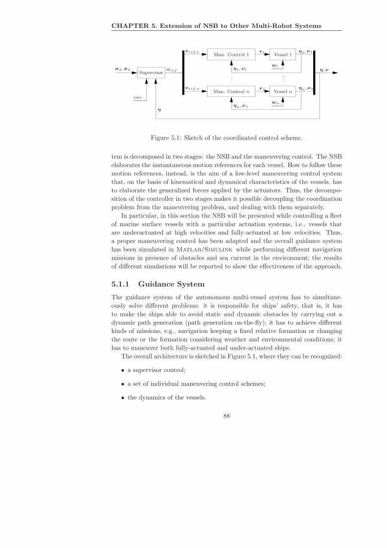
CHAPTER 5. Extension of NSB to Other Multi-Robot Systems
σd, σdSupervisor
vref
vref,1Man. Control 1
τ1Vessel 1
w1
η1, ν1
η1, ν1
.
.
....
vref,nMan. Control n
τnVessel n
wn
ηn, νn
ηn, νn
η, ν
η
env
Figure 5.1: Sketch of the coordinated control scheme.
tem is decomposed in two stages: the NSB and the maneuvering control. The NSB
elaborates the instantaneous motion references for each vessel. How to follow these
motion references, instead, is the aim of a low-level maneuvering control system
that, on the basis of kinematical and dynamical characteristics of the vessels, has
to elaborate the generalized forces applied by the actuators. Thus, the decompo-
sition of the controller in two stages makes it possible decoupling the coordination
problem from the maneuvering problem, and dealing with them separately.
In particular, in this section the NSB will be presented while controlling a fleet
of marine surface vessels with a particular actuation systems, i.e., vessels that
are underactuated at high velocities and fully-actuated at low velocities. Thus,
a proper maneuvering control has been adapted and the overall guidance system
has been simulated in Matlab/Simulink while performing different navigation
missions in presence of obstacles and sea current in the environment; the results
of different simulations will be reported to show the effectiveness of the approach.
5.1.1 Guidance System
The guidance system of the autonomous multi-vessel system has to simultane-
ously solve different problems: it is responsible for ships’ safety, that is, it has
to make the ships able to avoid static and dynamic obstacles by carrying out a
dynamic path generation (path generation on-the-fly); it has to achieve different
kinds of missions, e.g., navigation keeping a fixed relative formation or changing
the route or the formation considering weather and environmental conditions; it
has to maneuver both fully-actuated and under-actuated ships.
The overall architecture is sketched in Figure 5.1, where they can be recognized:
• a supervisor control;
• a set of individual maneuvering control schemes;
• the dynamics of the vessels.
88
5.1 NSB for a Fleet of Marine Surface Vessels
The supervisor can be seen as a dynamical path planner that, based on sensor
information, defines the motion reference directives for each vessel. In particular,
it can use information concerning the absolute/relative positions of the vessels of
the fleet (e.g., from GPS systems/scanning sonars), information about the environ-
ment (integration of maps and sensor information) or other kind of measurements
(wind, current, traffic condition, etc.) to take high-level decisions and define the
motion directives for the vessel of the fleet. Moreover, the motion coordination
among multiple vessels requires a consistent exchange of information among the
vessels. Thus, the necessity to manage highly structured data and the high traffic
of information makes the supervisor usually work at low frequency.
The maneuvering control is aimed at making each vessel following the motion
directives received by the supervisor. To this purpose, it uses information from
inertial navigation systems, gyroscopes, accelerometers and compasses to define
the generalized force applied by the actuators. Depending on the controller, an
estimation of the dynamic model can be used to improve the performance of the
control action. Managing non structured information data, this controller can
work at higher frequency than the supervisor.
Following the previous considerations, while simulating an autonomous multi-
vessels system the complexity of the system can became drastically elevate. Thus,
depending on the desired accuracy of the system and depending on the aim of
the simulation, some effects can be neglected, e.g., the non-linear terms of the
dynamic model of the vessels, or the sensors’ noise or the sensors’ sampling time.
Moreover, the working frequency of the supervisor and the maneuvering control
can be considered equal, and the characteristics of the environment (maps) or of
the vessel (dynamic models) used for the control purposes can be supposed exactly
known.
In the specific case, the supervisor implements the NSB control while the ma-
neuvering controls applies a control law derived from [38]. Moreover, the con-
trollers are supposed working at different sampling times; the dynamic model is
that one presented in Chapter 2 and it supposed exactly known; while the environ-
mental disturbances are dynamically estimated by the maneuvering controllers.
5.1.2 Actuation System
As explained in Section 2.2.3, depending on the characteristics of the generalized
propulsion force applied by their actuation system (represented by the vector τ of
eq. (2.14)), the vessels can be classified in fully-actuated or under-actuated. In this
section, the case of surface vessels that are under-actuated at high velocities and
fully-actuated at low velocities is considered. The only relevant types of vessels to
be considered in this class are the ones which become underactuated in the sway
direction at hight speed. These vessels are typically equipped with a number of
tunnel thrusters, designed to assist at low-speed maneuvers, which are inoperable
89
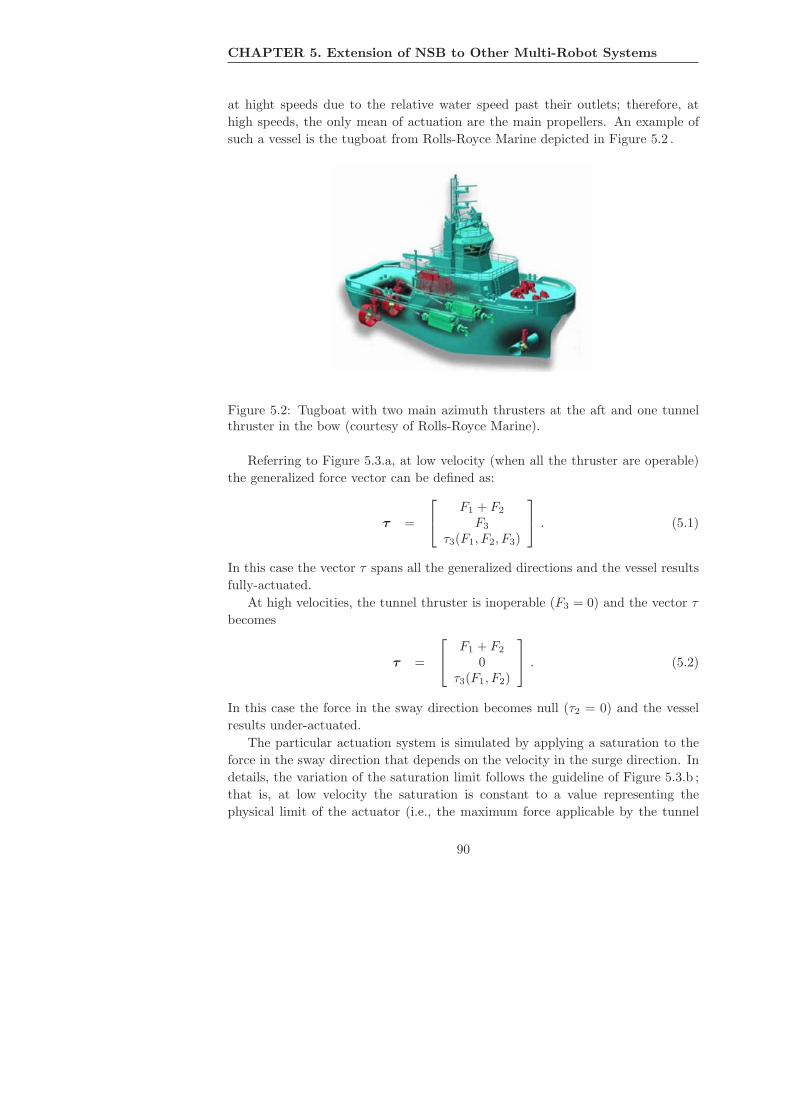
CHAPTER 5. Extension of NSB to Other Multi-Robot Systems
at hight speeds due to the relative water speed past their outlets; therefore, at
high speeds, the only mean of actuation are the main propellers. An example of
such a vessel is the tugboat from Rolls-Royce Marine depicted in Figure 5.2 .
Figure 5.2: Tugboat with two main azimuth thrusters at the aft and one tunnelthruster in the bow (courtesy of Rolls-Royce Marine).
Referring to Figure 5.3.a, at low velocity (when all the thruster are operable)
the generalized force vector can be defined as:
τ =
F1 + F2
F3
τ3(F1, F2, F3)
. (5.1)
In this case the vector τ spans all the generalized directions and the vessel results
fully-actuated.
At high velocities, the tunnel thruster is inoperable (F3 = 0) and the vector τ
becomes
τ =
F1 + F2
0τ3(F1, F2)
. (5.2)
In this case the force in the sway direction becomes null (τ2 = 0) and the vessel
results under-actuated.
The particular actuation system is simulated by applying a saturation to the
force in the sway direction that depends on the velocity in the surge direction. In
details, the variation of the saturation limit follows the guideline of Figure 5.3.b ;
that is, at low velocity the saturation is constant to a value representing the
physical limit of the actuator (i.e., the maximum force applicable by the tunnel
90
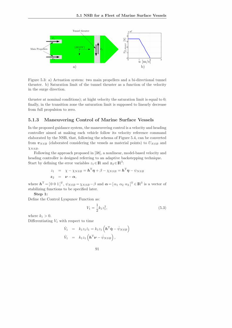
5.1 NSB for a Fleet of Marine Surface Vessels
Main Propellers
Tunnel thruster
F1
F2
F3
{BODY }
0 1 2 30
1
2
3
4
x 104
u [m/s]
τ 2,m
ax
[N]
a) b)
Figure 5.3: a) Actuation system: two main propellers and a bi-directional tunnelthruster. b) Saturation limit of the tunnel thruster as a function of the velocityin the surge direction.
thruster at nominal conditions); at hight velocity the saturation limit is equal to 0;
finally, in the transition zone the saturation limit is supposed to linearly decrease
from full propulsion to zero.
5.1.3 Maneuvering Control of Marine Surface Vessels
In the proposed guidance system, the maneuvering control is a velocity and heading
controller aimed at making each vehicle follow its velocity reference command
elaborated by the NSB, that, following the schema of Figure 5.4, can be converted
from vNSB (elaborated considering the vessels as material points) to UNSB and
χNSB .
Following the approach proposed in [38], a nonlinear, model-based velocity and
heading controller is designed referring to an adaptive backstepping technique.
Start by defining the error variables z1∈ IR and z2∈ IR3:
z1 = χ− χNSB = hTη + β − χNSB = hTη − ψNSB
z2 = ν − α,
where hT = [ 0 0 1 ]T, ψNSB =χNSB−β and α= [α1 α2 α3 ]T ∈ IR3 is a vector of
stabilizing functions to be specified later.
Step 1:
Define the Control Lyapunov Function as:
V1 =1
2k1z
21 , (5.3)
where k1 > 0.
Differentiating V1 with respect to time
V1 = k1z1z1 = k1z1
(hTη − ψNSB
)
V1 = k1z1
(hTν − ψNSB
),
91
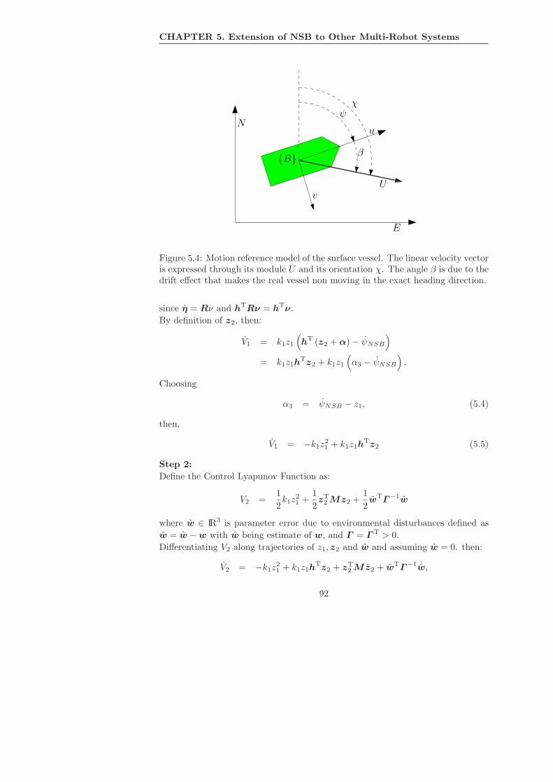
CHAPTER 5. Extension of NSB to Other Multi-Robot Systems
N
E
U
ψ
u
v
χ
β{B}
Figure 5.4: Motion reference model of the surface vessel. The linear velocity vectoris expressed through its module U and its orientation χ. The angle β is due to thedrift effect that makes the real vessel non moving in the exact heading direction.
since η = Rν and hTRν = hTν.
By definition of z2, then:
V1 = k1z1
(hT (z2 + α) − ψNSB
)
= k1z1hTz2 + k1z1
(α3 − ψNSB
).
Choosing
α3 = ψNSB − z1, (5.4)
then,
V1 = −k1z21 + k1z1h
Tz2 (5.5)
Step 2:
Define the Control Lyapunov Function as:
V2 =1
2k1z
21 +
1
2zT
2 Mz2 +1
2wTΓ−1w
where w ∈ IR3 is parameter error due to environmental disturbances defined as
w = w − w with w being estimate of w, and Γ = Γ T > 0.
Differentiating V2 along trajectories of z1,z2 and w and assuming w = 0. then:
V2 = −k1z21 + k1z1h
Tz2 + zT2 Mz2 + wTΓ−1 ˙w,
92

5.1 NSB for a Fleet of Marine Surface Vessels
since M = MT and ˙w = ˙w.
Since
Mz2 = M (ν − α)
= τ − N(ν)ν + RT(ψ)w − Mα
then:
V2 = −k1z21 + zT
2
(hk1z1 + τ − Nν + RT w − Mα
)+ wTΓ−1 ˙w.
Being ν = z2 + α and w = w − w, then:
V2 = −k1z21 − zT
2 Nz2 + zT2
(hk1z1 + τ − Nα + RT w − Mα
)
+wTΓ−1(
˙w − ΓRz2
).
Assigning
τ = Mα + Nα − RT w − hk1z1 − K2z2 (5.6)
where K2 > 0, and choosing:˙w = ΓRz2 (5.7)
then:
V2 = −k1z21 − zT
2 (N + K2)z2. (5.8)
As stated in [62], since the system is persistently excited, choosing smooth
α1, α1, α2, α2 ∈ L∞ then the proposed control and disturbance adaption law makes
the origin of the error system [z1,z2, w] UGAS/ULES.
The choice of α1, α2 depends on the actuation system of the vessels, i.e., when
the vessel is fully-actuated
α1 = UNSB cosβNSB
α2 = UNSB sinβNSB ;
while when the vessel is under-actuated
α1 = UNSB cosβNSB
and α2 is defined such as τ2 = 0.
The proposed controller guarantees that z1, z2 go to zero, and that w converges
to w. Thus, the vessel velocity converges to the desired values {UNSB , χNSB}only when the vessel is fully-actuated; for an underactuated vessel, instead, u
converges to UNSB cosβNSB while v is uncontrolled. It is worth noting that,
while an underactuated ship executes a straight motion at cruise speed it is U =√u2 + v2 ≃ u since the sway velocity v is much smaller than u; on the other hand,
when v cannot be neglected with respect to u (as, e.g., in turning maneuvers)
93

CHAPTER 5. Extension of NSB to Other Multi-Robot Systems
it is U =
√(UNSB cosβNSB)
2+v2. Nevertheless, in real applications, ships move
using way-point tracking and turning maneuvers are used for short time periods to
adjust changes of course; thus, the convergence properties of the proposed control
law are acceptable in practice.
When implementing the control law (5.6) it is important to avoid expressions
involving the time derivatives of the states. To this purpose, the time derivative
of the stabilizing function α is conveniently computed by differentiating along the
trajectories of the states [59]. Moreover, to obtain high-order derivatives of ψNSB
in (5.4), it is worth noticing that ψNSB is defined as ψNSB = χNSB−β, where
χNSB is the reference input obtained by the NSB and β is measured using GPS
velocities. Thus, the high-order derivatives ψNSB , ψNSB are computed through a
low-pass filter.
5.1.4 Simulation Package
Following the control architecture scheme of Figure 5.1, a software package that
simulates an autonomous multi-vessel system has been implemented in the Mat-
lab/Simulink environment (see Figures 5.5 and 5.6). The simulator, presented
in [19], allows the user to test the supervisory control approach and the single-
vehicle maneuvering control schemes in a number of missions. In particular, the
software is aimed at simulating an autonomous fleet of surface vessels performing
navigation missions in complex realistic environment.
The control architecture is implemented using both Simulink blocks and Mat-
lab functions. The Simulink model of Figure 5.5 reproduces the block scheme of
Figure 5.1, while the subsystem of Figure 5.6 shows major details on the maneu-
vering control architecture. In these figures it is possible to recognize continuous
and discrete blocks (e.g., continuous integrators, zero-order holders, discrete deriv-
ative), non-linear blocks (e.g., saturations and dead-zones), and calls to Matlab
functions appropriately built (e.g., Maneuvering control, Dynamic Model). More-
over, the different colors of the signals lines represent different sampling frequen-
cies.
The simulator presents a graphical interface (shown in Figure 5.7), developed
with the Matlab Graphical User Interface (GUI), that allows the user to dy-
namically define all the parameters of the mission and the characteristics of the
environment. The user can define on screen the initial configuration of the fleet,
the sub-tasks of the mission and their gains, the presence and the entity of envi-
ronmental forces. For example, the user can define the formation that the vessels
have to keep during the navigation, the desired trajectory of the barycenter of the
fleet, the gains and the priorities of the single tasks of the mission.
To simulate complex realistic mission, the presence of obstacles is also taken
into account; the user can interactively insert both punctual and continuous ob-
94

5.1 NSB for a Fleet of Marine Surface Vessels
Figure 5.5: Simulink implementation: Control scheme.
Figure 5.6: Simulink implementation: Maneuvering control + Vessels dynamicssubsistem.
95
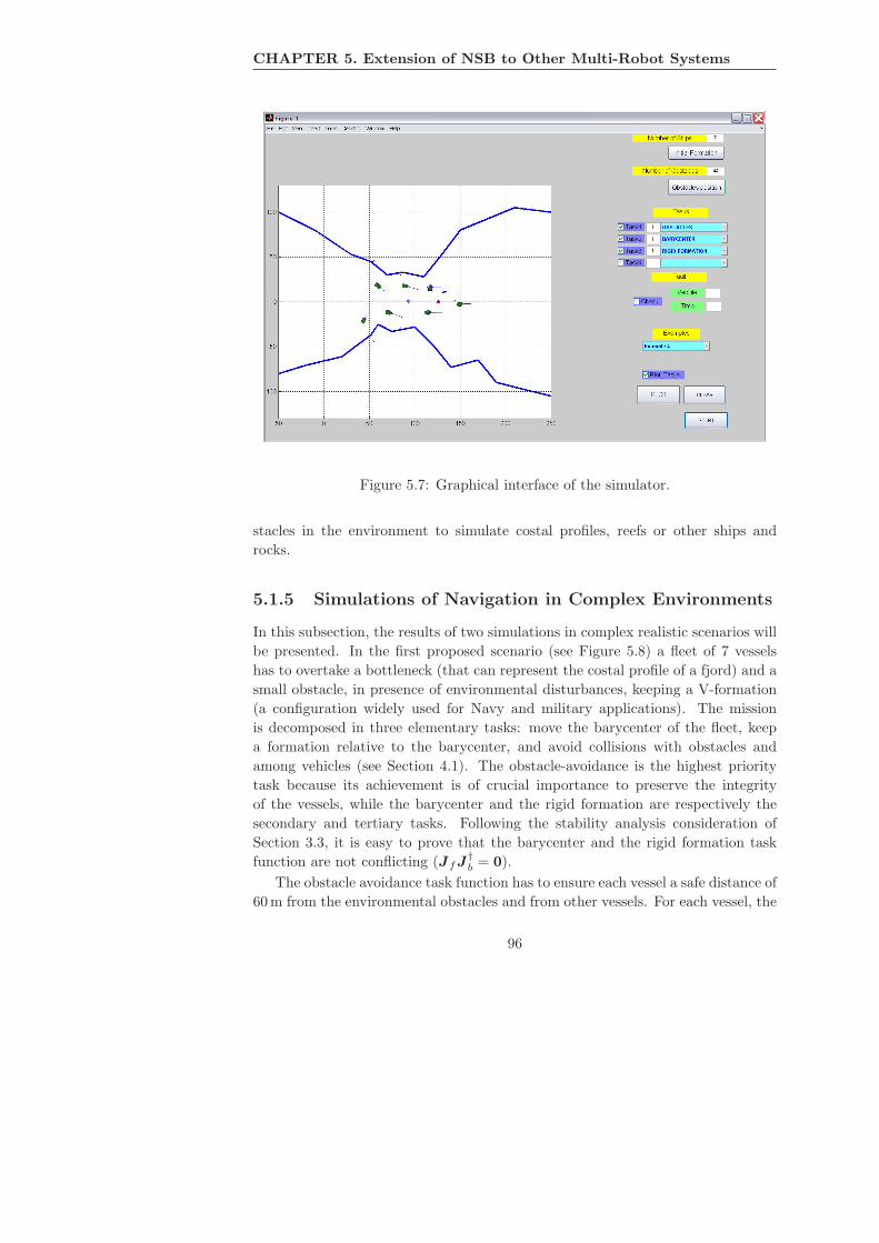
CHAPTER 5. Extension of NSB to Other Multi-Robot Systems
Figure 5.7: Graphical interface of the simulator.
stacles in the environment to simulate costal profiles, reefs or other ships and
rocks.
5.1.5 Simulations of Navigation in Complex Environments
In this subsection, the results of two simulations in complex realistic scenarios will
be presented. In the first proposed scenario (see Figure 5.8) a fleet of 7 vessels
has to overtake a bottleneck (that can represent the costal profile of a fjord) and a
small obstacle, in presence of environmental disturbances, keeping a V-formation
(a configuration widely used for Navy and military applications). The mission
is decomposed in three elementary tasks: move the barycenter of the fleet, keep
a formation relative to the barycenter, and avoid collisions with obstacles and
among vehicles (see Section 4.1). The obstacle-avoidance is the highest priority
task because its achievement is of crucial importance to preserve the integrity
of the vessels, while the barycenter and the rigid formation are respectively the
secondary and tertiary tasks. Following the stability analysis consideration of
Section 3.3, it is easy to prove that the barycenter and the rigid formation task
function are not conflicting (JfJ†b = 0).
The obstacle avoidance task function has to ensure each vessel a safe distance of
60 m from the environmental obstacles and from other vessels. For each vessel, the
96
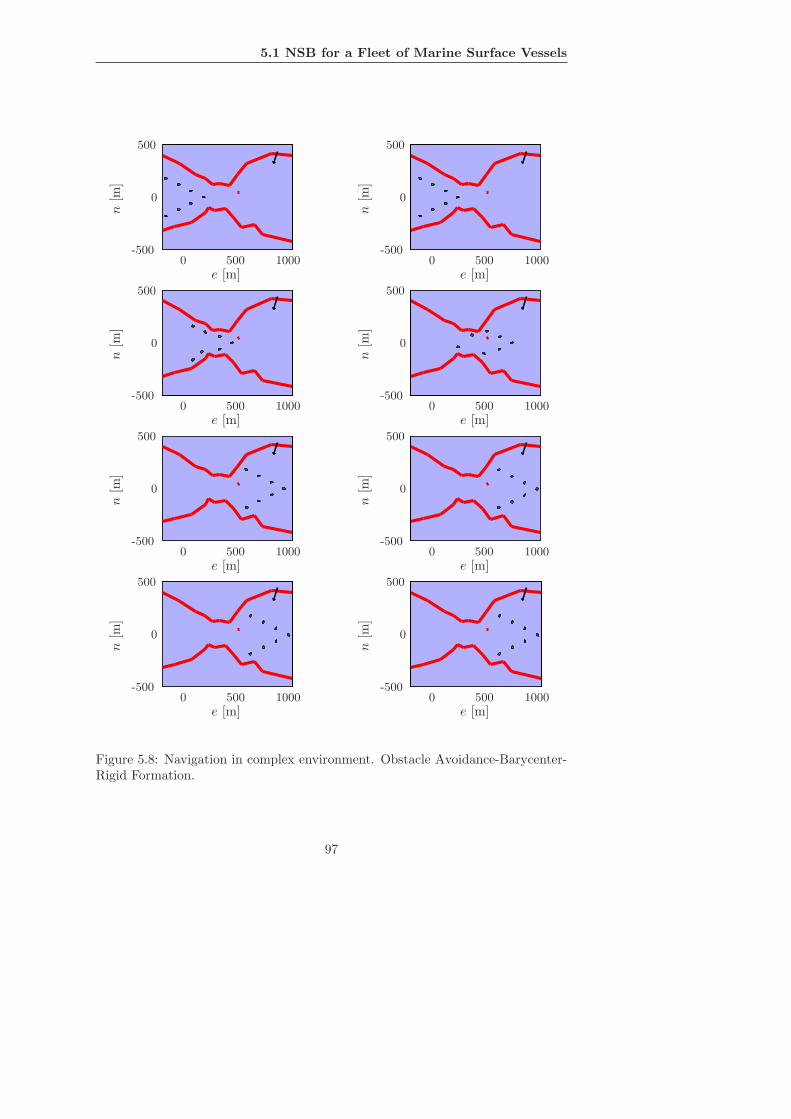
5.1 NSB for a Fleet of Marine Surface Vessels
n[m
]
n[m
]
n[m
]
n[m
]
n[m
]
n[m
]
n[m
]
n[m
]
e [m]e [m]
e [m]e [m]
e [m]e [m]
e [m]e [m]
0
0
0
0
0
0
0
0
0
0
0
0
0
0
0
0
-500-500
-500-500
-500-500
-500-500
500
500
500
500
500
500
500
500
500
500
500
500
500
500
500
500
10001000
10001000
10001000
10001000
Figure 5.8: Navigation in complex environment. Obstacle Avoidance-Barycenter-Rigid Formation.
97

CHAPTER 5. Extension of NSB to Other Multi-Robot Systems
task function is activated only when the distance from environmental obstacles or
other vessels becomes lower than 60 m. When the vessel is simultaneously close to
(i.e., under 60 m from) multiple obstacles, then the closest obstacle has the highest
priority. Since a moving obstacle is assumed to be more dangerous than a fixed
one, if the vessel is simultaneously close to an environmental obstacle and another
vessel, the avoidance of the other vessel takes higher priority if the distance from
it is greater than the distance from the environmental obstacle multiplied by a
gain chosen (by trial and error) equal to 0.3 .
0 200 400 600 800 1000−150
−100
−50
0
50
100
150
σf
t[s]
d
0 500 1000 1500 2000−10
0
10
20
30
40
σb
t[s]
c
0 200 400 600 800 1000−5
0
5
10
15
20
25
30
σo
t[s]
b
0 500 1000−500
0
500a
n[m
]
e [m]
Figure 5.9: a) Paths followed by the ships; b) error of the obstacle avoidance taskfunction; c) error of the barycenter task function; d) error of the rigid formationtask function.
The desired trajectory of the barycenter is a rectilinear segment that connects
the initial position [ 0 0 ]T m to the final position [ 800 0 ]T m according to a fifth-
order polynomial time law of 700 s duration with null initial and final velocity. The
vessels have to attain and keep a V-formation around the barycenter and, once
reached the final configuration, the vessels has to keep the formation and orient
themselves in the opposite direction to the current. The gain matrices of the
barycenter task function and of the rigid formation task function are respectively
98
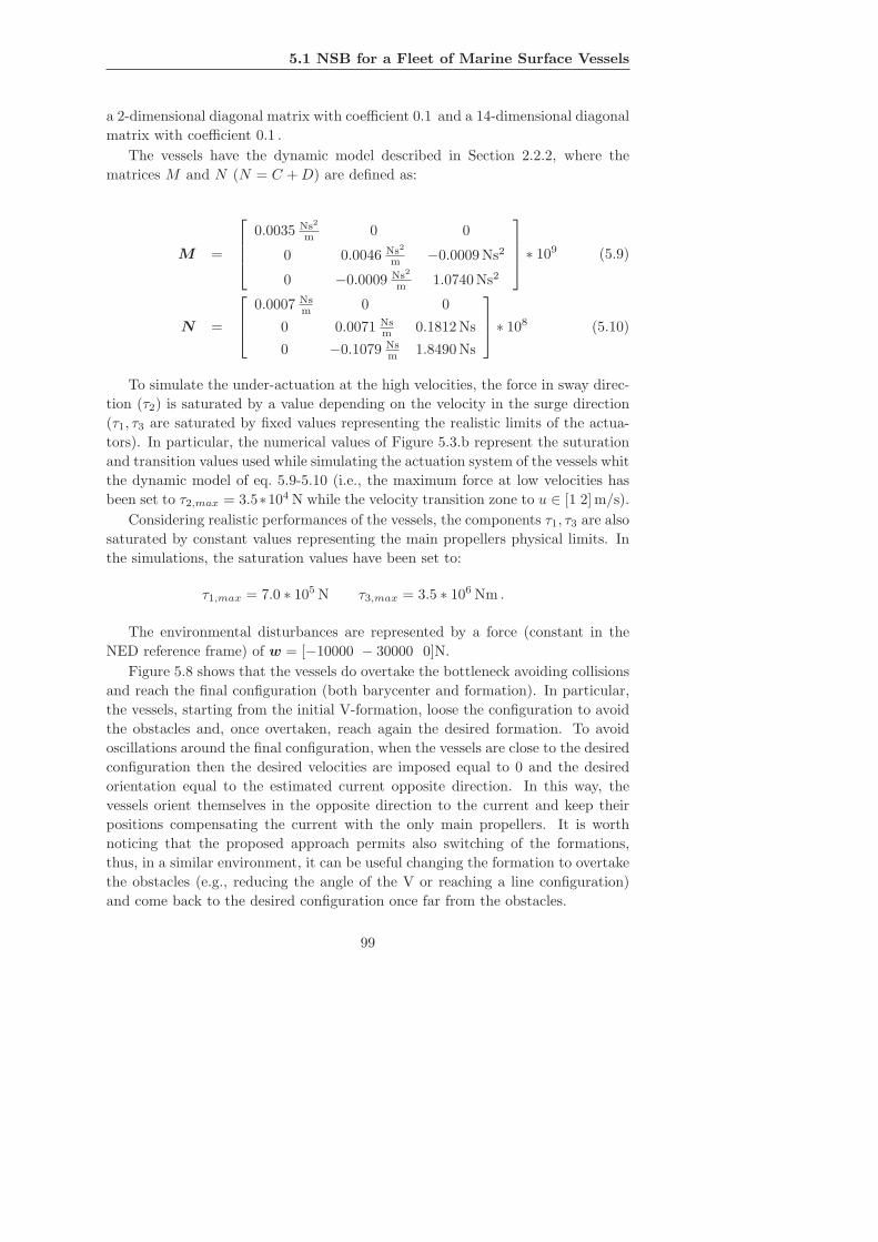
5.1 NSB for a Fleet of Marine Surface Vessels
a 2-dimensional diagonal matrix with coefficient 0.1 and a 14-dimensional diagonal
matrix with coefficient 0.1 .
The vessels have the dynamic model described in Section 2.2.2, where the
matrices M and N (N = C +D) are defined as:
M =
0.0035 Ns2
m 0 0
0 0.0046 Ns2
m −0.0009Ns2
0 −0.0009 Ns2
m 1.0740Ns2
∗ 109 (5.9)
N =
0.0007 Nsm 0 0
0 0.0071 Nsm 0.1812Ns
0 −0.1079 Nsm 1.8490Ns
∗ 108 (5.10)
To simulate the under-actuation at the high velocities, the force in sway direc-
tion (τ2) is saturated by a value depending on the velocity in the surge direction
(τ1, τ3 are saturated by fixed values representing the realistic limits of the actua-
tors). In particular, the numerical values of Figure 5.3.b represent the suturation
and transition values used while simulating the actuation system of the vessels whit
the dynamic model of eq. 5.9-5.10 (i.e., the maximum force at low velocities has
been set to τ2,max = 3.5∗104 N while the velocity transition zone to u ∈ [1 2] m/s).
Considering realistic performances of the vessels, the components τ1, τ3 are also
saturated by constant values representing the main propellers physical limits. In
the simulations, the saturation values have been set to:
τ1,max = 7.0 ∗ 105 N τ3,max = 3.5 ∗ 106 Nm .
The environmental disturbances are represented by a force (constant in the
NED reference frame) of w = [−10000 − 30000 0]N.
Figure 5.8 shows that the vessels do overtake the bottleneck avoiding collisions
and reach the final configuration (both barycenter and formation). In particular,
the vessels, starting from the initial V-formation, loose the configuration to avoid
the obstacles and, once overtaken, reach again the desired formation. To avoid
oscillations around the final configuration, when the vessels are close to the desired
configuration then the desired velocities are imposed equal to 0 and the desired
orientation equal to the estimated current opposite direction. In this way, the
vessels orient themselves in the opposite direction to the current and keep their
positions compensating the current with the only main propellers. It is worth
noticing that the proposed approach permits also switching of the formations,
thus, in a similar environment, it can be useful changing the formation to overtake
the obstacles (e.g., reducing the angle of the V or reaching a line configuration)
and come back to the desired configuration once far from the obstacles.
99
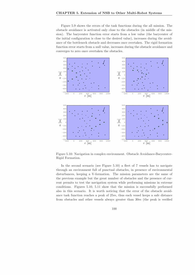
CHAPTER 5. Extension of NSB to Other Multi-Robot Systems
Figure 5.9 shows the errors of the task functions during the all mission. The
obstacle avoidance is activated only close to the obstacles (in middle of the mis-
sion). The barycenter function error starts from a low value (the barycenter of
the initial configuration is close to the desired value), increases during the avoid-
ance of the bottleneck obstacle and decreases once overtaken. The rigid formation
function error starts from a null value, increases during the obstacle avoidance and
converges to zero once overtaken the obstacles.
−200 0 200 400 600 800 1000−500
−400
−300
−200
−100
0
100
200
300
400
500
−200 0 200 400 600 800 1000−500
−400
−300
−200
−100
0
100
200
300
400
500
−200 0 200 400 600 800 1000−500
−400
−300
−200
−100
0
100
200
300
400
500
−200 0 200 400 600 800 1000−500
−400
−300
−200
−100
0
100
200
300
400
500
n[m
]
n[m
]
n[m
]
n[m
]
e [m]e [m]
e [m]e [m]
Figure 5.10: Navigation in complex environment. Obstacle Avoidance-Barycenter-Rigid Formation.
In the second scenario (see Figure 5.10) a fleet of 7 vessels has to navigate
through an environment full of punctual obstacles, in presence of environmental
disturbances, keeping a V-formation. The mission parameters are the same of
the previous example but the great number of obstacles and the presence of cur-
rent permits to test the navigation system while performing missions in extreme
conditions. Figures 5.10, 5.11 show that the mission is successfully performed
also in this scenario. It is worth noticing that the error of the obstacle avoid-
ance task function reaches a peak of 25m, thus each vessel keeps a safe distance
from obstacles and other vessels always greater than 30m (the peak is verified
100
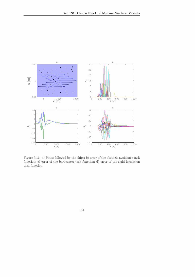
5.1 NSB for a Fleet of Marine Surface Vessels
0 200 400 600 800 1000−60
−40
−20
0
20
40
60
σf
t[s]
d
0 500 1000 1500 2000−20
−15
−10
−5
0
5
10
15
σb
t[s]
c
0 200 400 600 800 10000
5
10
15
20
25
30
σo
t[s]
b
0 500 1000−500
0
500a
n[m
]
e [m]
Figure 5.11: a) Paths followed by the ships; b) error of the obstacle avoidance taskfunction; c) error of the barycenter task function; d) error of the rigid formationtask function.
101

CHAPTER 5. Extension of NSB to Other Multi-Robot Systems
when a vessel is simultaneously close to an obstacle and another vessel). Fig-
ure 5.12.a) shows that the estimation of the current w does converge to the real
value w = [−10000 − 30000 0]N while Figure 5.12.b) shows that in the final con-
figuration all the ships orient themselves in the opposite direction to the current.
Videos of the performed simulations can be found in the cd attached to the thesis
(file: vessel 1.avi vessel 2.avi) or at the Author’s webpage at:
http://webuser.unicas.it/arrichiello
0 500 1000 1500 2000 2500−3
−2
−1
0
1
2
3
4
5x 10
4τ [N]
a)
0 500 1000 1500 2000 2500−3
−2
−1
0
1
2
θ [rad]
b)
t [s]t [s]
Figure 5.12: a) Current estimation; b) Orientation of the ships.
5.2 NSB for Mobile Ad-hoc NETworks
5.2.1 The MANET Case
Another kind of application concerns the control of wireless Mobile Ad-hoc NET-
works (MANETs). In particular, the MANET is a collection of autonomous nodes
that communicate each other without using any fixed networking infrastructure.
Each node in a MANET operates as both a host and a router. Therefore, any
node can communicate directly with nodes that are within its transmission range
and, in order to reach a node that is out of its range, data packets are relayed
over a sequence of intermediate nodes using a store-and-forward multi-hop trans-
mission principle. The MANET approach is very attractive for on-field mobile
robots applications where often the task execution may compromise the robot-
base communication as, e.g., in a survey and rescue mission to be performed
inside a damaged building or in exploration of unknown areas. For this reason, a
number of researchers have started proposing MANET-based solutions for mobile
robot communication (see, e.g.,[47, 116, 134]). However, these solutions, as tra-
ditional MANET implementations, consider position and motion of each node as
uncontrollable variables. Assuming instead that at least some of the nodes may
102

5.2 NSB for Mobile Ad-hoc NETworks
be controlled, more performing MANETs can be designed. Indeed, a suitable dy-
namic reconfiguration of the robots’ position allows to adapt the coverage area of
the communication network to better support the team’s mission, to avoid signal
fading area (e.g., that induced by the presence of obstacles), and to handle possible
fault of some team members.
This class of problems has been recently addressed in some works. In ref-
erence [105] an algorithm that enables a group of cooperating mobile robots to
establish and maintain a wireless ad-hoc network is proposed; specifically, each ro-
bot defines its local optimal trajectory by minimizing a functional that accounts for
network connectivity, obstacle avoidance and other aspects of interest. A behavior-
based architecture is proposed in [129] to encourage a team of robots to maintain
a local communication network while exploring a given area. An algorithm that,
starting from an arbitrary initial connected condition, modifies the robots’ location
to achieve a fault-tolerant bi-connected configuration is proposed in [27].
A general formulation for the coverage problem is proposed in [46], where a
distributed asynchronous algorithm is developed to dynamically reconfigure a mo-
bile sensors network taking into account sensor performance; specifically, in this
approach the control input of each vehicle is proportional to the distance from its
actual position and the centroid of the associated Voronoi region. In reference [28],
to guarantee communication for a mobile robot involved into a dynamic coverage
problem, a static network of markers is autonomously dispersed by the robot dur-
ing its motion (these markers are also used to improve localization capability). In
reference [105] cooperative communication, i.e., enable to a group of mobile robot
to establish and maintain a wireless ad-hoc network, is achieved thorough a distrib-
uted approach where each robot defines its local optimal trajectory by minimizing
a functional that accounts for network connectivity, obstacle avoidance and other
aspects of interest. An algorithm that, starting from an arbitrary initial connected
condition, modifies the robots’ location to achieve a fault-tolerant bi-connected
configuration is proposed in [27]. A rendezvous algorithm for coordinated motion
of mobile robots with limited mobility and communication constraints is proposed
in [86]; in this approach, network connectivity is guaranteed imposing to each
robot, at each sample time, to move toward the circum-center defined by itself
and its neighbors and restricting the travel distance. Recovery behaviors to au-
tonomously re-establish communication after a failure between some or all of the
nodes in the network are discussed in [127].
In this section, the problem of dynamically adapting the configuration of a
platoon of mobile robots equipped with a wireless device (that will be called an-
tennas) so as to realize a MANET supporting communication of an autonomously
driven vehicle (that will be called robot) with a fixed base station will be con-
sider. Antennas coordination for robot coverage is achieved in the framework of
the NSB approach presented in the previous sections, by resorting to properly
defined task functions. This approach has shown to be efficient and reliable in si-
103

CHAPTER 5. Extension of NSB to Other Multi-Robot Systems
multaneous handling of several control objectives, namely, robot-antennas-station
connectivity, obstacle avoidance and fault tolerance of the mobile antennas (as
shown in [9, 11, 10]).
5.2.2 Problem Statement
The algorithm described in the Chapter 3 can be used to suitably coordinate the
motion of a set of mobile antennas so as to implement a MANET that dynamically
adapts its coverage area (see Figure 5.13). Specifically, in the following a platoon
of n mobile antennas that must ensure the communication between a mobile agent
executing its mission and a fixed base station (e.g., an Internet access point) is
considered. Of course, the mobile agent and the antennas have also to avoid the
obstacles eventually present in the environment.
base station
mobile antennas
agent
Figure 5.13: Sketch of the coverage problem to be solved; the autonomous agentneeds to be connected with the base station by the use of a platoon of mobileantennas.
Let’s denote with the subscript i the generic antenna as well as the agent, i.e.,
it is i ∈ [0, n+1] where i = 0 denotes the base station and i = n+1 denotes the
agent. Each antenna is supposed to cover in open space a circular area Ii centered
in pi and of radius
rmax,i = rmax,i (i, pwi) , (5.11)
104

5.2 NSB for Mobile Ad-hoc NETworks
where pwi is the current level of power used for transmission. It can be noticed
that rmax,i depends on the characteristic of the i-th antenna. Moreover, it depends
also on the level of power used for transmission pwi. During the execution of a
mission the level of power used for the transmission may be varied in order to
preserve the battery level or, on the other side, can be decreased when the battery
level is low.
In order to guarantee adequate operative margins, we will constraint each an-
tenna to dialogue in a smaller region, identified via the radius
dmax,i = (1 −∆) rmax,i 0 < ∆ < 1 , (5.12)
where ∆ is a design parameter. Notice that, in presence of obstacles, it is pos-
sible to decrease dmax,i to take into account the possible reduced propagation.
Moreover, in order to avoid collisions, all other bodies in the environment (i.e.,
base station, other antennas, agent and obstacles) must be farther than dmin,i
from each antenna. Notice that this definition is similar to that of comfort zone
in [129], therefore, this term will be used in the following to denote the area shown
in Figure 5.14.
antenna
dmin
dmax
rmax
Figure 5.14: Comfort zone of an antenna and relevant distances.
Then, at time t the i-th vehicle is able to directly communicate with all vehicles
which are inside the region Ii(t). The set of all direct communication paths con-
stitutes a graph that can be synthetically represented via the associated incidence
matrix G whose entries satisfy
gij =
{1 if pj ∈ Ii
0 otherwise .
105
CHAPTER 5. Extension of NSB to Other Multi-Robot Systems
Notice that, since pi∈/ Ii, it results gii = 0 by definition.
If all the antennas have the same transmission’s characteristics and are using
the same level of power, then G is a symmetric matrix, otherwise this may not be
the case.
Let’s introduce the communication matrix C(t) defined as
C(t) = G(t) + G2(t) + · · · + Gn(t) ∀t , (5.13)
where the i-th row of the k-th term in the sum represents the set of all the vehicles
that at time t can be reached by a message generated by the i-th vehicle in exactly
k hops.
It is immediate to recognize that bi-directional communication between the
i-th and the j-th vehicles is guaranteed if and only if the product
cij(t) · cji(t) 6= 0 . (5.14)
Notice that the value assumed by cij represents a crude measurement of the
degree of redundancy for the related communication channel; indeed it represents
the number of different paths existing among the i-th and the j-th vehicles.
Our goal is to guarantee the presence of a radio bridge between the agent and
the base station, i.e.,
c0 n+1(t) · cn+1 0(t) 6= 0 ∀t , (5.15)
while the agent to be covered performs its own mission moving along unknown
trajectories.
5.2.3 The Proposed Algorithm
Let’s define as virtual chain a virtual connection that, starting from the base
station reaches all the n antennas. The agent is connected, if ∃i : pn+1 ∈ Ii, i.e.,
if it belongs to the comfort zone of one of the antennas in the virtual chain. We
impose to the antennas to autonomously self-arrange in order to create a proper
virtual chain or, in other words, that the matrix C satisfies (5.15).
Let’s define a n-dimensional vector k that collects the indexes of the antennas
in their order from the base station. Thus, kj (i.e., the j-th component of vector k)
is the index that identifies the antenna at the j-th place —not necessarily the j-th
antenna— and kj , kj+1 index two consecutive vehicles along the circle. As will be
described in Subsection 5.2.4, the vector k may be modified at each sample time.
Let’s define as T the time step of the algorithm, i.e., the time needed to compute
the new reference velocity for all the antennas and as Tc the communication time,
i.e., the time needed to communicate between two generic antennas. It is required
that T > Tc. Moreover, each antenna has a maximum velocity denoted as vmax,i.
The following assumptions are made:
106

5.2 NSB for Mobile Ad-hoc NETworks
• Tcvmax,i ≪ dmin,i , i.e., the configuration of the antennas can be considered
as constant during the communication among them;
• Tvmax,i ≪ dmin,i , i.e., the movement is slow with respect to the distance
dmin;
• The environment is considered as known; the information can be available
from an off-line map or acquired on-line by resorting to sensor fusion tech-
niques;
• At the initial time, the virtual chain is correctly formed (see Subsection 5.2.4).
The coverage problem described in Section 5.2 can be solved by resorting to
the technique described in Section 3, using the reasonable assumptions above. It
is necessary to properly define the task functions and properly arrange them in a
priority order. It is worth noticing that the priority is dynamic, in the sense that
a supervisor (Figure 3.4) is in charge of modifying the relative priorities among
the tasks based on the comments below.
The task functions to be achieved by the antennas in order of decreasing pri-
ority, being 1 the highest and assuming that k0 is the base station, are:
• for an antenna along the virtual chain kj with j ∈ {1, n−1}:
1. avoid the obstacles;
2. keep the next antenna kj+1 in the comfort zone;
3. keep the previous antenna kj−1 in the comfort zone.
• for the last antenna in the virtual chain kn:
1. avoid the obstacles;
2. keep the previous antenna kj−1 in the comfort zone.
Moreover, for the antenna closest to the agent (not necessarily kn), the task
of keeping the agent in the comfort zone is considered with a priority lower than
the obstacle avoidance and higher than the others. With respect to the above list,
thus, this task is at a priority 2 while the other tasks from priority 2 skip of one
unity downward.
The agent to be covered might move independently from the antennas such as,
e.g., in case of a human. Notice that it is possible that it pulls them away too far
from the base station when, e.g., the antennas are all stretched in a line but the
agent is still moving away. Better performance can be achieved if the agent is a
robot and it is included as a part of the platoon to be coordinated. This may be
achieved by imposing to the robot the following task function:
1. avoid the obstacles;
107

CHAPTER 5. Extension of NSB to Other Multi-Robot Systems
2. reach a goal or track a path.
that, when the robot is close to the limit of the comfort zone, needs to be modified
in:
1. avoid the obstacles;
2. stay within the comfort zone of the closest antenna;
3. reach a goal or track a path.
As extensively verified in simulation, when the robot is close to the limit of the
comfort zone, this formulation imposes on the robot some kind of stop and wait
command until the antennas, after a self reconfiguration, are able to accommodate
further motion. In this way, any break in the communication bridge is prevented
but, obviously, it is not ensured that the robot reaches its goal position. In case
of absence of obstacles this means that, at most, the robot can stretches all the
antennas in a line and then stop, preventing its movement outside the coverage
area.
The task function aimed at ensuring connection of the chain is
σc =n∑
i=1
σc,i , (5.16)
where σc,i ∈ IR provides connection of the antenna i at position kj to the previous
one as
σc,i =
‖r‖ if ‖r‖≤dmin
0 if dmin<‖r‖<dmax
‖r‖ if ‖r‖≥dmax
(5.17)
with r=pkj−pkj−1
and
Jc,i =
{0 if σc,i =0
rT otherwise .
According to the above definition, the desired value for the task function is selected
as:
σd,i =
dmin if ‖r‖≤dmin
0 if dmin<‖r‖<dmax
dmax if ‖r‖≥dmax .
(5.18)
In a similar way, it is also possible to define the task so as to impose connection
between kj and kj+1.
Obstacle avoidance is achieved by using a properly defined task function that,
for a generic antenna kj is given by:
σo,l =∥∥∥pkj
− po,l
∥∥∥ , (5.19)
108

5.2 NSB for Mobile Ad-hoc NETworks
where po,l is the vector representing the closest point of the obstacle to the an-
tenna (similarly to Section 3.7). The limit of this obstacle avoidance approach,
common to all the path planning algorithm relying on local information only, is the
possibility to get trapped in local minima. Further details can be found in [14, 15].
Once the task function have been defined, it is possible to compute the error
variable to output the reference velocities for the specific task. Further applying
eq. (3.7) allow to implement the singularity robust task priority inverse kinematics
algorithm and compose the finale, reference, velocity for each of the antennas.
5.2.4 Dynamic Handling of the Virtual Chain
As mentioned before, in order to guarantee the proper connection between the
agent and the base station, the antennas dynamically self-organize to realize a
virtual chain. This configuration is obtained using the follow algorithm:
1 from the base station k0 look for the closest antenna inside I0
and label it as the first in the virtual chain k1; make k1 the
current antenna;
2 from the current antenna in the virtual chain kj look for the
closest antenna inside Ikjin the remaining antennas and label
it as the successive in the virtual chain kj+1; make kj+1 the
current antenna;
3 repeat the point 2 increasing the index of the current antenna
until there is no remaining antenna; if j + 1 = n go to step 5,
else keep the virtual chain formed at tk−1, i.e., k(tk) := k(tk−1)
4 virtually connect the agent to its closest antenna (not
necessarily kn).
It is algoritmically proven that, with the implemented kinematic control, start-
ing from a connected virtual chain and keeping this chain for all the mission, the
connection is never broken. In fact, if the antenna in position kj-th is moving out-
side the comfort area of the kj−1-th antenna the associated velocity component is
immediately nullified because in (3.7) it is projected in to the null of pseudo-inverse
associated with the connection task function (5.18).
It is worth noticing that the simplest case is given by a static virtual chain,
i.e., the order of the antennas is never changed during a mission.
5.2.5 Simulation Results
The proposed algorithm, aimed at guaranteing the wireless communication bridge
between the agent and the base station by means of several mobile antennas, has
been extensively tested in numerical simulations. In all the simulations run the
109

CHAPTER 5. Extension of NSB to Other Multi-Robot Systems
agent is a robot, i.e, it performs its missions independently from the antennas, i.e.,
the algorithm acquires its trajectory in real-time. Moreover, the robot’s move-
ments are coordinated with the MANET so that it can eventually receive stop
to allow reconfiguration of the antennas. Notice that, as explained above, this
behavior is done autonomously by considering the proposed kinematic control and
not explicitly commanded to the robot. In this section, two case studies will be re-
ported corresponding to two different environments. For the simulations reported
the following parameters have been used
rmax,i = 24m
dmax,i = 16m
dmin,i = 6m
T = 300ms
while the maximum velocities are 1 m/s for the robot and 1.5 m/s for the antennas.
All the NSB gains have been set to 0.5. It can be noticed that dmax,i has been
kept constant ∀i. In both case studies the robot moves in an environment with
obstacles and it is required that it stays at a minimum distance of 10 m from them.
In the first scenario the robot has to reach a goal position in presence of two line-
shaped obstacles in the environment. The simulation starts with the 7 antennas
randomly distributed around the base station following an uniform distribution
centered in position [0 0]T m with an interval of 50 m on the coordinates and
verifying that a virtual chain is formed and the robot in position [10 10]T m. The
robot has to reach a goal in position [0 110]T m. The antennas have to ensure
the communication between the robot and the base station avoiding collisions with
walls, robot, base station and among themselves. Figure 5.15 reports six snapshots
of the mission execution; the robot moves to the final goal in about 120 s and the
antennas do ensure the communication coverage during all the motion. Notice that
the virtual serial chain among the antennas can dynamically change during the
mission, giving more flexibility to the approach; moreover, differently from [27],
this implies that there is no need to impose an explicit order to the antennas.
The second scenario simulates a navigation in a building with several rooms.
The robot has to reach different goals passing through predefined via-points and,
obviously, avoiding the walls. The simulation starts with the 10 antennas randomly
distributed around the base station following an uniform distribution centered in
position [0 0]T m with an interval of 50 m on the coordinates and verifying that a
virtual chain is formed and the robot in the initial position [10 10]T m. Figure 5.16
reports several snapshots of the mission execution. The antennas do maintain the
coverage with the base station during all the mission and avoid the obstacles
themselves. During the simulation, the robot sometimes can reach the boundary
of the area covered by the nearest antenna; in these cases the robot stops and
waits for reconfiguration of the network.
110

5.2 NSB for Mobile Ad-hoc NETworks
Videos of the performed simulations can be found in the cd attached to the thesis
(files: MANET building.avi MANET obstacles.avi) or at the Author’s webpage
at: http://webuser.unicas.it/arrichiello
t = 0.3 t = 24 t = 48
t = 72 t = 96 t = 120
111
111
22
2
222
33
3
3
33
444
444
555
555
666
666
77
7
7
77
Figure 5.15: Snapshots of a coverage mission for a platoon of mobile antennas inpresence of 2 linear-shaped obstacles. The robot (blue dot) has to reach the goal(marked by a ×), while the antennas (red dots) have to ensure connection betweenthe robot and the fixed station (the star).
111

CHAPTER 5. Extension of NSB to Other Multi-Robot Systems
t = 0.3 t = 138 t = 276
t = 414 t = 561 t = 690
111
111
222
222
333
333
444
444
555
555
6
6
6
66
6
77
7
7
77
8
8
8
8
8
8
999
999
101010
101010
Figure 5.16: Snapshots of a coverage mission for a platoon of mobile antennasin a complex environment. The robot (blue dot) has to reach the several goals(marked by a ×), while the antennas (red dots) have to ensure connection betweenthe robot and the fixed station (the star).
112

Chapter 6
Conclusions
The research described in this thesis has concerned the control of multi-robot
systems. After a brief overview on the state of the art of the research in the
field, a behavior-based approach to control generic multi-robot systems, namely
the Null-Space-based Behavioral control, has been presented and tested in experi-
mental and simulative case studies. In particular, the NSB has been introduced in
comparison with the main behavioral approaches known in literature (the layered
control system as a significant case of competitive approach and the motor schema
control as a significant case of cooperative approach) to underline its novelty and
advantages. The NSB, in fact, differs from the other approaches in the way it
composes the single task outputs to build the motion command to the robots,
and, properly managing the tasks organized in a hierarchical structure, it permits
to simultaneously achieve multiple, even-conflicting, tasks.
The NSB has been widely tested in experimental and simulative case studies
concerning different multi-robot systems. In particular, it has been experimen-
tally tested while controlling a platoon of wheeled grounded mobile robots (the
7 Khepera II robots available at the Laboratorio di Automazione Industriale of the
University of Cassino) while achieving several formation control missions. More-
over, it has been simulated in the Matlab/Simulink environment while controlling
typologically different kinds of multi-robot systems (i.e., a fleet of marine surface
vessels and a platoon of mobile antennas).
The experimental and simulative results prove the effectiveness and the flexibil-
ity of the approach. The NSB, in fact, can be applied to different kinds of vehicles
by decoupling the guidance system from the maneuvering controls of the specific
vehicles. That is, the NSB elaborates the motion directive for each vehicle of the
team ignoring their kinematical and dynamical structures, while the maneuvering
controls make the single vehicles following the relative motion references.
Moreover, the NSB results applicable to different typologies of missions. In
fact, it has been shown that, by properly defining the task functions, it is possible
113
CHAPTER 6. Conclusions
to control the distribution of the robots in the environment, to navigate with a
fixed formation or to perform missions like the escorting/entrapment or the control
of MANETs.
As it has been shown, the NSB results robust to sensor noise (the experiments
have been performed with a real set-up that obviously presents noisy measure-
ment), to external disturbances (e.g., the sea current in the marine surface vessels
case) and to dynamic changing environment (e.g., dynamic obstacles and moving
targets during the experiments with the platoon of Khepera II). Moreover, the
NSB results dynamically scalable to the adding or removing of robots from the
system (as it has been shown in the entrapment experiment with the team of
Khepera II).
All these considerations allow to consider the NSB approach effective and ro-
bust for the control of different multi-robot systems. However, several extensions
and improvements can be taken into consideration. The first step for future re-
search is toward a decentralization of the approach, that is, making the robots
more autonomous and avoiding or reducing the communication with the remote
unit. Until now, the NSB has been implemented while controlling robots (the
Khepera II) with limited elaboration capabilities, mechanical performances (they
can move only on a really flat surface), sensor equipment (the infrared sensors on
board of each robot are too noisy to be used for localization and mapping) and
communication capabilities (the Bluetooth turrets do not permit a direct com-
munication among the robots and do not allow the simultaneous communication
among the remote unit and more then 7 robots). Improving the experimental set-
up (e.g., using the new Khepera III robots instead of the Khepera II), it is possible
to overtake most of these limits. The Khepera III robot, in fact, has a more pow-
erful processor, can move on a more irregular surface, can use Wireless Ethernet
communication (that presents larger bandwidth and ideally does not have any lim-
its on the maximum number of robots in the network), and have a better sensor
equipment. Thus, with an upgrade of the experimental set-up, it will be possible to
go out form the flat arena used for the performed experiments and maybe navigate
in the building. To do this, it is necessary to decentralize the control algorithm,
deal with communication networks problems and make the robots using their own
sensors to localize themselves in the environment (thus dealing with problems like
multi-robot SLAM). Moreover, future research on the NSB may concern the def-
inition of other task functions (e.g., organize an exploration mission by means of
the NSB) and the experimental validation of NSB approach for the MANET case
mission and for the fleet of marine vessels (hopefully continuing the collaboration
with the Norwegian University of Science and Technology in Trondheim).
114

Bibliography
[1] http://www.k-team.com/. K-Team.
[2] G. Antonelli. Underwater robots. Motion and force control of vehicle-
manipulator systems. Springer Tracts in Advanced Robotics, Springer-
Verlag, Heidelberg, D, 2nd edition, June 2006.
[3] G. Antonelli, F. Arrichiello, and S. Chiaverini. Experimental kinematic com-
parison of behavioral approaches for mobile robots. In Proceedings 16th IFAC
World Congress, Prague, CZ, July 2005.
[4] G. Antonelli, F. Arrichiello, and S. Chiaverini. The Null-Space-based Behav-
ioral control for mobile robots. In Proceedings 2005 IEEE International Sym-
posium on Computational Intelligence in Robotics and Automation, pages
15–20, Espoo, Finland, June 2005.
[5] G. Antonelli, F. Arrichiello, and S. Chiaverini. The Null-Space-based Be-
havioral control for soccer-playing mobile robots. In Proceedings 2005
IEEE/ASME International Conference on Advanced Intelligent Mechatron-
ics, pages 1257–1262, Monterey, CA, July 2005.
[6] G. Antonelli, F. Arrichiello, and S. Chiaverini. Experiments of formation con-
trol with collisions avoidance using the Null-Space-based Behavioral control.
In Proceedings 14th Mediterranean Conference on Control and Automation,
Ancona, I, June 2006.
[7] G. Antonelli, F. Arrichiello, and S. Chiaverini. The Null-Space-based Behav-
ioral control for autonomous robotic systems. Journal of Intelligence Service
Robotics, in press, 2007.
[8] G. Antonelli, F. Arrichiello, S. Chiaverini, and K. J. Rao. Preliminary exper-
iments of formation control using the Null-Space-based Behavioral control.
In Proceedings 8th IFAC Symposium on Robot Control, Bologna, I, Sept.
2006.
115
BIBLIOGRAPHY
[9] G. Antonelli, F. Arrichiello, S. Chiaverini, and R. Setola. A self-configuring
MANET for coverage area adaptation through kinematic control of a platoon
of mobile robots. In Proceedings 2005 IEEE/RSJ International Conference
on Intelligent Robots and Systems, pages 1332–1337, Edmonton, CA, Aug.
2005.
[10] G. Antonelli, F. Arrichiello, S. Chiaverini, and R. Setola. Coordinated con-
trol of mobile antennas for ad-hoc networks. International Journal of Mod-
elling Identification and Control Special/Inaugural issue on Intelligent Robot
Systems, 1(1):63–71, 2006.
[11] G. Antonelli, F. Arrichiello, S. Chiaverini, and R. Setola. Coordinated con-
trol of mobile antennas for ad-hoc networks in cluttered environments. In
Proceedings 9th International Conference on Intelligent Autonomous Sys-
tems (IAS-9), Tokyo, J, March 2006.
[12] G. Antonelli and S. Chiaverini. Fuzzy redundancy resolution and motion co-
ordination for underwater vehicle-manipulator systems. IEEE Transactions
on Fuzzy Systems, 11(1):109–120, 2003.
[13] G. Antonelli and S. Chiaverini. Kinematic control of a platoon of autonomous
vehicles. In Proceedings 2003 IEEE International Conference on Robotics
and Automation, pages 1464–1469, Taipei, TW, Sept. 2003.
[14] G. Antonelli and S. Chiaverini. Obstacle avoidance for a platoon of au-
tonomous underwater vehicles. In Proceedings 6th IFAC Conference on Ma-
noeuvring and Control of Marine Craft, pages 143–148, Girona, E, Sept.
2003.
[15] G. Antonelli and S. Chiaverini. Fault tolerant kinematic control of platoons
of autonomous vehicles. In Proceedings 2004 IEEE International Conference
on Robotics and Automation, pages 3313–3318, New Orleans, LA, April 2004.
[16] G. Antonelli and S. Chiaverini. Kinematic control of platoons of autonomous
vehicles. IEEE Transactions on Robotics, 22(6):1285–1292, Dec. 2006.
[17] R.C. Arkin. Motor schema based mobile robot navigation. The International
Journal of Robotics Research, 8(4):92–112, 1989.
[18] R.C. Arkin. Behavior-Based Robotics. The MIT Press, Cambridge, MA,
1998.
[19] F. Arrichiello and S. Chiaverini. A simulation package for coordinated mo-
tion control of a fleet of under-actuated surface vessels. In Proceedings 5th
MATHMOD Conference, Vienna, Austria, March. 2006.
116

BIBLIOGRAPHY
[20] F. Arrichiello, S. Chiaverini, and T.I. Fossen. Formation control of marine
surface vessels using the Null-Space-based Behavioral control. In Group
Coordination and Cooperative Control, K.Y. Pettersen, T. Gravdahl, and H.
Nijmeijer (Eds.), Springer-Verlag’s Lecture Notes in Control and Information
Systems series, pages 1–19. May 2006.
[21] F. Arrichiello, S. Chiaverini, and T.I. Fossen. Formation control of under-
actuated surface vessels using the Null-Space-based Behavioral control. In
Proceedings 2006 IEEE/RSJ International Conference on Intelligent Robots
and Systems, pages 5942–5947, Beijing, China, Oct. 2006.
[22] H. Asama, A. Matsumoto, and Y. Ishida. Design Of An Autonomous And
Distributed Robot System: Actress. Proceedings IEEE/RSJ International
Workshop on Intelligent Robots and Systems’ 89.(IROS’89), pages 283–290,
1989.
[23] T. Bailey and H. Durrant-Whyte. Simultaneous localization and mapping
(SLAM): part I. IEEE Robotics and Automation Magazine, 13(2):99–110,
June 2006.
[24] T. Bailey and H. Durrant-Whyte. Simultaneous localization and mapping
(SLAM): part II. IEEE Robotics and Automation Magazine, 13(3):108– 117,
Sept. 2006.
[25] T. Balch and R.C. Arkin. Behavior-based formation control for multiro-
bot teams. IEEE Transactions on Robotics and Automation, 14(6):926–939,
1998.
[26] D. Barnes and J. Gray. Behaviour synthesis for co-operant mobile robot
control. In Proceedings 1991 International Conference on Control, pages
1135–1140, 1991.
[27] P. Basu and J. Redi. Movement control algorithms for realization of fault-
tolerant ad hoc robot networks. IEEE Network, 18(4):36–44, 2004.
[28] M.A. Batalin and G.S. Sukhatme. Coverage, exploration and deployment by
a mobile robot and communication network. Telecommunication Systems –
Special Issue on Wireless Sensor Networks, 26(2):181–196, 2004.
[29] R.W. Beard, J. Lawton, and F.Y. Hadaegh. A coordination architecture
for spacecraft formation control. IEEE Transactions on Control Systems
Technology, 9(6):777–790, 2001.
[30] R.W. Beard, T.W. McLain, D.B. Nelson, D. Kingston, and D. Johanson. De-
centralized cooperative aerial surveillance using fixed-wing miniature UAVs.
Proceedings of the IEEE, 94(7):1306–1324, July 2006.
117

BIBLIOGRAPHY
[31] C. Belta and V.K. Kumar. Abstraction and control of groups of robots.
IEEE Transactions on Robotics, 20(5):865–875, 2004.
[32] G. Beni. The concept of cellular robotic system. Proceedings IEEE Interna-
tional Symposium on Intelligent Control, pages 57–62, 1988.
[33] B.E. Bishop. On the use of redundant manipulator techniques for control
of platoons of cooperating robotic vehicles. IEEE Transactions on Systems,
Man and Cybernetics, 33(5):608–615, Sept. 2003.
[34] B.E. Bishop and D.J. Stilwell. On the application of redundant manipulator
techniques to the control of platoons of autonomous vehicles. In Proceedings
2001 IEEE International Conference on Control Applications, pages 823–
828, Mexico City, MX, Sept. 2001.
[35] A. Bloch, J. Baillieul, and P. Crouch. Nonholonomic Mechanics and Control.
Springer, 2003.
[36] J. Borenstein and Y. Koren. Real-time obstacle avoidance for fast mobile
robots. IEEE Transactions on Systems, Man and Cybernetics, 19:1179–1187,
1989.
[37] E. Borhaug, A. Pavlov, R. Ghabcheloo, K. Pettersen, A. Pascoal, and C. Sil-
vestre. Formation control of underactuated marine vehicles with communi-
cation constraints,. In Proceedings 7th IFAC Conference on Manoeuvring
and Control of Marine Craft, Lisbon, P, 2006.
[38] M. Breivik and T.I. Fossen. A unified concept for controlling a marine surface
vessel through the entire speed envelope. In Proceedings 2005 IEEE Interna-
tional Symposium on Mediterrean Conference on Control and Automation,
pages 1518–1523, Limassol, Cyprus, June 2005.
[39] R.A. Brooks. A robust layered control system for a mobile robot. IEEE
Journal of Robotics and Automation, 2:14–23, 1986.
[40] W. Burgard, M. Moors, C. Stachniss, and F.E. Schneider. Coordinated
multi-robot exploration. IEEE Journal of Robotics, 21(3):376–386, June
2005.
[41] Y.U. Cao, A.S. Fukunaga, and A.B. Kahng. Robot colonies. Special Is-
sue of Autonomous Robots, volume 4, chapter Cooperative Mobile Robot-
ics:Antecedents and Directions. R.C. Arkin and G.A. Bekey, (Eds.), Kluwer
Academic Publisher, March 1997.
[42] S. Carpin and L.E. Parker. Cooperative motion coordination amidst dynamic
obstacles. Distributed Autonomous Robotic Systems, 5:145–154, 2002.
118

BIBLIOGRAPHY
[43] L. Chaimowicz, B. Grocholsky, J.F. Keller, V. Kumar, and C.J. Taylor.
Experiments in Multirobot Air-Ground Coordination. Proceedings of the
IEEE International Conference on Robotics and Automation, page 4053,
2004.
[44] P. Chiacchio, S. Chiaverini, L. Sciavicco, and B. Siciliano. Closed-loop in-
verse kinematics schemes for constrained redundant manipulators with task
space augmentation and task priority strategy. The International Journal
Robotics Research, 10(4):410–425, 1991.
[45] S. Chiaverini. Singularity-robust task-priority redundancy resolution for
real-time kinematic control of robot manipulators. IEEE Transactions on
Robotics and Automation, 13(3):398–410, 1997.
[46] J. Cortes, S. Martınez, T. Karatas, and F. Bullo. Coverage control for
mobile sensing networks. IEEE Transactions on Robotics an Automation,
20(2):243–255, 2004.
[47] A. Das, J. Spletzer, V. Kumar, and C. Taylor. Ad hoc network for local-
ization and control. In Proceedings 41st IEEE Conference on Decision and
Control, pages 2978–2983, Las Vegas, NE, Dec. 2002.
[48] A.K. Das, R. Fierro, V. Kumar, J.P. Ostrowski, J. Spletzer, and C.J. Taylor.
A vision-based formation control framework. IEEE Transactions on Robotics
and Automation, 18(5):813–825, 2002.
[49] A. De Luca and G. Oriolo. Modelling and control of nonholonomic mechan-
ical systems, volume 360 of CISM Courses and Lectures, pages 277–342.
Springer, 1995.
[50] A. De Luca, G. Oriolo, and M. Vendittelli. Stabilization of the unicycle via
dynamic feedback linearization. In 6th IFAC Symposium on Robot Control,
pages 397–402, Wien, A, Sept. 2000.
[51] J.P. Desai, V. Kumar, and J.P. Ostrowski. Control of changes in formation
for a team of mobile robots. In Proceedings 1999 IEEE International Con-
ference on Robotics and Automation, pages 1556–1561, Detroit, MI, May
1999.
[52] G. Dudek, M.R.M. Jenkin, E. Milios, and D. Wilkes. A taxonomy for multi-
agent robotics. Autonomous Robots, 3(4):375–397, 1996.
[53] P. Encarnacao and A. Pascoal. Combined trajectory tracking and path fol-
lowing for marine craft. Proceedings 9th Mediterranean Conference on Con-
trol and Automation, 2001.
119

BIBLIOGRAPHY
[54] A. Farinelli, L. Iocchi, and D. Nardi. Multirobot Systems: A Classification
Focused on Coordination. IEEE Transactions on Systems Man and Cyber-
netics Part B(Cybernetics), 34(5):2015–2028, 2004.
[55] J.A. Fax and R.M. Murray. Information flow and cooperative control of
vehicle formations. IEEE Transactions on Automatic Control, 49(9):1465–
1476, 2004.
[56] J.T. Feddema, C. Lewis, and D.A. Schoenwald. Decentralized control of
cooperative robotic vehicles: theory and application. IEEE Transactions on
Robotics and Automation, 18(5):852–864, 2002.
[57] E. Fiorelli, N.E. Leonard, P. Bhatta, D. Paley, R. Bachmayer, and D.M.
Fratantoni. Multi-auv control and adaptive sampling in monterey bay. In
Proceedings IEEE Autonomous Underwater Vehicles 2004: Workshop on
Multiple AUV Operations, pages 134–147, Sebasco, ME, June 2004.
[58] T.I. Fossen. Guidance and Control of Ocean Vehicles. Chichester New York,
1994.
[59] T.I. Fossen. Marine Control Systems: Guidance, Navigation and Control
of Ships, Rigs and Underwater Vehicles. Marine Cybernetics, Trondheim,
Norway, 2002.
[60] T.I. Fossen. A nonlinear unified state-space model for ship maneuvering and
control in a seaway. Journal of Bifurcation and Chaos, 2005.
[61] T.I. Fossen, M. Breivik, and R. Skjetne. Line-of-sight path following of
underactuated marine craft. In Proceedings 2003 IFAC Conference on Ma-
neuvering and Control of Marine Craft, Girona, Spain, September 2003.
[62] T.I. Fossen, A. Loria, and A. Teel. A theorem for ugas and ules of (passive)
nonautonomous systems: Robust control of mechanical systems and ships.
International Journal of Robust and Nonlinear Control, JRNC-11:95–108,
2001.
[63] T.I. Fossen and J.P. Strand. Nonlinear passive weather optimal positioning
control (WOPC) system for ships and rigs: experimental results. Automat-
ica, 37(5):701–715, 2001.
[64] T. Fukuda and S. Nakagawa. Dynamically reconfigurable robotic system.
Proceedings 1988 IEEE International Conference on Robotics and Automa-
tion, pages 1581–1586, 1988.
120
BIBLIOGRAPHY
[65] T. Fukuda, S. Nakagawa, Y. Kawauchi, and M. Buss. Structure decision
method for self organising robots based on cellstructures-CEBOT. Pro-
ceedings 1989 IEEE International Conference on Robotics and Automation,
pages 695–700, 1989.
[66] E. Gat, R. Desai, R. Ivlev, J. Loch, and D.P. Miller. Behavior control for
robotic exploration of planetary surfaces. IEEE Transactions on Robotics
and Automation, 10(4):490–503, 1994.
[67] B.P. Gerkey and M.J. Mataric. A formal framework for the study of task al-
location in multi-robot systems. International Journal of Robotics Research,
23(9):939–954, 2004.
[68] A. Howard, L.E. Parker, and G.S. Sukhatme. Experiments with a Large
Heterogeneous Mobile Robot Team: Exploration, Mapping, Deployment
and Detection. The International Journal of Robotics Research, 25(5-6):431,
2006.
[69] T. Huntsberger, P. Pirjanian, A. Trebi-Ollennu, H. Das Nayar, H. Aghaz-
arian, AJ Ganino, M. Garrett, SS Joshi, and PS Schenker. CAMPOUT: a
control architecture for tightly coupled coordination of multirobot systems
for planetary surface exploration. IEEE Transactions on Systems, Man and
Cybernetics, Part A, 33(5):550–559, 2003.
[70] I.A.F. Ihle, J. Jouffroy, and T.I. Fossen. Robust Formation Control of Marine
Craft using Lagrange Multipliers. In Group Coordination and Cooperative
Control, K.Y. Pettersen, T. Gravdahl, and H. Nijmeijer (Eds.), Springer-
Verlag’s Lecture Notes in Control and Information Systems series. May 2006.
[71] I.A.F. Ihle, R. Skjetne, and T.I. Fossen. Nonlinear formation control of
marine craft with experimental results. In Proceedings 43rd IEEE Conference
on Decision and Control, volume 1, pages 680–685, Paradise Island, The
Bahamas, Dec 2004.
[72] I.I. Kaminer, O.A. Yakimenko, V.N. Dobrokhodov, M.I. Lizarraga, and A.M.
Pascoal. Cooperative control of small UAVs for naval applications. Proceed-
ings 43rd IEEE Conference on Decision and Control, 1, 2004.
[73] B. M. Kim and P. Tsiotras. Controllers for unicycle-type wheeled robots:
theoretical results and experimental validation. IEEE Transactions on Ro-
botics and Automation, 18(3):294–307, June 2002.
[74] H. Kitano. RoboCup Rescue: a grand challenge for multi-agent systems.
Proceedings Fourth International Conference on MultiAgent Systems, pages
5–12, 2000.
121
BIBLIOGRAPHY
[75] H. Kitano, M. Asada, Y. Kuniyoshi, I. Noda, and E. Osawa. RoboCup: The
Robot World Cup Initiative. Proceedings of the first international conference
on Autonomous agents, pages 340–347, 1997.
[76] E. Klavins. Communication complexity of multi-robot systems. Algorithmic
Foundations of Robotics V, 7:275–292, 2003.
[77] I. Kolmanovsky and N.H. McClamroch. Developments in nonholonomic con-
trol problems. IEEE Control System Magazine, 15(6):20–36, 1995.
[78] K. Konolige, D. Fox, C. Ortiz, A. Agno, M. Eriksen, B. Limketkai, J. Ko,
B. Morisset, D. Schulz, B. Stewart, et al. Centibots: Very large scale distrib-
uted robotic teams. Experimental Robotics: The 9th International Sympo-
sium, Springer Tracts in Advanced Robotics (STAR). Springer Verlag, 2005.
[79] C.R. Kube and H. Zhang. Collective robotics: from social insects to robots.
Adaptive Behavior, 2(2):189–218, 1993.
[80] D. Langer, J.K. Rosenblatt, and M. Hebert. A behavior-based system
for off-road navigation. IEEE Transactions on Robotics and Automation,
10(6):776–783, 1994.
[81] J.C. Latombe. Robot Motion Planning. Kluwer Academic Publishers, 1990.
[82] E.L. Lefeber, K.Y. Pettersen, and H. Nijmeijer. Tracking control of an
underactuated ship. IEEE Transactions on Control Systems Technology,
11(1):52–61, 2003.
[83] A. Loria, T.I. Fossen, and E. Panteley. A separation principle for dynamic
positioning of ships: theoretical and experimental results. IEEE Transac-
tions on Control Systems Technology, 8(2):332–343, 2000.
[84] A.A. Maciejewski. Numerical filtering for the operation of robotic manip-
ulators through kinematically singular configurations. Journal of Robotic
Systems, 5(6):527–552, 1988.
[85] J.A. Marshall, T. Fung, M.E. Broucke, G.M.T. DEleuterio, and B.A. Francis.
Experiments in multirobot coordination. Robotics and Autonomous Systems,
54(3):265–275, 2006.
[86] S. Martınez, J. Cortes, and F. Bullo. On robust rendezvous for mobile
autonomous agents. In 16th IFAC World Congress, Praha, CZ, July 2005.
[87] M.J. Mataric. Designing emergent behaviors: From local interaction to col-
lective intelligence. In Proceedings of the International Conference on Simu-
lation of Adaptive Behavior: From Animal to Animal, pages 432–441, 1992.
122

BIBLIOGRAPHY
[88] M.J. Mataric. Issues and approaches in the design of collective autonomous
agents. Robotics and Autonomous Systems, 16(2):321–331, 1995.
[89] M.J. Mataric. Behavior-based control: Examples from navigation, learn-
ing, and group behavior. Journal of Experimental and Theoretical Artificial
Intelligence, 9(2-3):323–336, 1997.
[90] M.J. Mataric, M. Nilsson, and K.T. Simsarian. Cooperative multi-robot
box-pushing. Proceedings of the 1995 IEEE/RSJ International Conference
on Intelligent Robots and Systems, pages 556–561, 1995.
[91] Y. Nakamura, H. Hanafusa, and T. Yoshikawa. Task-priority based redun-
dancy control of robot manipulators. The International Journal Robotics
Research, 6(2):3–15, 1987.
[92] F.R. Noreils. Toward a robot architecture integrating cooperation between
mobile robots: application to indoor environment. International Journal of
Robotics Research, 12(1):79–98, 1993.
[93] F.R. Noreils and A.A. Recherche. Multi-Robot Coordination For Battlefield
Strategies. Proceedings of the 1992 lEEE/RSJ International Conference on
Intelligent Robots and Systems, 3, 1992.
[94] A. Oreback and H.I. Christensen. Evaluation of Architectures for Mobile
Robotics. Autonomous Robots, 14(1):33–49, 2003.
[95] G. Oriolo, A. De Luca, and M. Vendittelli. WMR control via dynamic
feedback linearization: design, implementation, and experimental validation.
IEEE Transactions on Control Systems Technology, 10(6):835–852, 2002.
[96] E. Pagello, A. D’Angelo, and E. Menegatti. Cooperation issue and distrib-
uted sensing for multirobot systems. Proceedings of the IEEE, 94(7):1370–
1383, July 2006.
[97] L. Pallottino, E.M. Feron, and A. Bicchi. Conflict Resolution Problems for
Air Traffic Management Systems Solved With Mixed Integer Programming.
IEEE Transaction on Intelligent Transportation Systems, 3(1):3, 2002.
[98] J. Park, Y. Choi, W.K. Chung, and Y. Youm. Multiple tasks kinematics
using weighted pseudo-inverse for kinematically redundant manipulators. In
Proceedings 2001 IEEE International Conference on Robotics and Automa-
tion, pages 4041–4047, Seoul, KR, May 2001.
[99] L.E. Parker. Designing control laws for cooperative agent teams. In Pro-
ceedings 1993 IEEE International Conference on Robotics and Automation,
volume 3, pages 582–587, Atlanta, GA, May 1993.
123
BIBLIOGRAPHY
[100] L.E. Parker. ALLIANCE: An architecture for fault tolerant, coopera-
tive control of heterogeneous mobile robots. In Proceedings of the 1994
IEEE/RSJ/GI International Conference on Intelligent Robots and Systems,
pages 776–783, Sept. 1994.
[101] L.E. Parker. On the design of behavior-based multi-robot teams. Advanced
Robotics, 10(6):547–578, 1996.
[102] L.E. Parker. The effect of heterogeneity in teams of 100+ mobile robots.
Multi-Robot Systems, 2003.
[103] K.Y. Pettersen and T.I. Fossen. Underactuated dynamic positioning of a
ship- experimental results. IEEE Transactions on Control Systems Technol-
ogy, 8(5):856–863, 2000.
[104] K.Y. Pettersen, F. Mazencs, and H. Nijmeijer. Global uniform asymp-
totic stabilization of an underactuated surface vessels: Experimental results.
IEEE Transactions on Control System Technology, 12(6):891–903, 2004.
[105] B. Pimentel and M. Campos. Cooperative communication in ad hoc net-
worked mobile robots. In Proceedings IEEE/RSJ International Conference
on Intelligent Robots and Systems, pages 2876–2881, Las Vegas, NE, Oct.
2003.
[106] P. Pirjanian. Multiple objective behavior-based control. Robotics and Au-
tonomous Systems, 31(1–2):53–60, April 2000.
[107] S.T. Pledgie, Y Hao, A.M. Ferreira, S.K. Agrawal, and R. Murphey. Groups
of unmanned vehicles: differential flatness, trajectory planning, and con-
trol. In Proceedings 2002 IEEE International Conference on Robotics and
Automation, pages 3461–3466, Washington, DC, May 2002.
[108] J.B. Pomet, B. Thuilot, G. Bastin, and G. Campion. A hybrid strategy
for the feedback stabilization of nonholonomicmobile robots. Proceedings
of 1992 IEEE International Conference on Robotics and Automation, pages
129–134, 1992.
[109] S. Premvuti and S. Yuta. Consideration on the cooperation of multiple
autonomous mobile robots. In Proceedings IEEE/RSJ International Con-
ference on Intelligent Robots and Systems, 1990.
[110] I. Rekleitis, G. Dudek, and E. Milios. Multi-robot collaboration for robust
exploration. Annals of Mathematics and Artificial Intelligence, 31(1):7–40,
2001.
[111] C. Reynolds. Flocks, herd and schools: A distributed behavioral model.
Computer Graphics, 21(4):25–34, 1987.
124
BIBLIOGRAPHY
[112] A. Saffiotti and Z. Wasik. A hierarchical behavior-based approach to ma-
nipulation tasks. In Proceedings of 2003 IEEE International Conference on
Robotics and Automation, pages 2780–2785, Taipei, Taiwan, Sept. 2003.
[113] C. Samson. Time-varying feedback stabilization of car-like wheeled mobile
robots. International Journal of Robotics Research, 12(1):55–64, 1993.
[114] M. Scheutz and V. Andronache. Architectural mechanisms for dynamic
changes of behavior selection strategies in behavior-based systems. IEEE
Transactions on Systems, Man and Cybernetics, 34(6):2377–2395, Dec. 2004.
[115] B. Seanor, Y. Gu, M.R. Napolitano, G. Campa, S. Gururajan, and L. Rowe.
3-aircraft formation flight experiments. In 14th Mediterranean Conference
on Control and Automation, Ancona,I, July 2006.
[116] G.T. Sibley, M.H. Rahmi, and G.S. Sukhatme. Robomote: A tiny mo-
bile robot platform for large-scale ad-hoc sensor networks. In Proceedings
IEEE International Conference on Robotics and Automation, pages 1143–
1148, Washington, DC, May 2002.
[117] B. Siciliano. Kinematic control of redundant robot manipulators: A tutorial.
Journal of Intelligent Robotic Systems, 3:201–212, 1990.
[118] R. Siegwart and I.R. Nourbakhsh. Introduction to Autonomous Mobile Ro-
bots. Bradford Book, 2004.
[119] R. Skjetne. The Maneuvering Problem. PhD.Thesis, Norwegian University
of Science and Technology, Trondheim, Norway, 2005.
[120] R. Skjetne, S. Moi, and T.I. Fossen. Nonlinear formation control of marine
craft. In Proceedings 41st IEEE Conference on Decision and Control, pages
1699–1704, Las Vegas, Nevada, USA, 2002.
[121] D.J. Stilwell and B.E. Bishop. Platoons of underwater vehicles. IEEE Con-
trol Systems Magazine, 20(6):45–52, 2000.
[122] D.J. Stilwell, B.E. Bishop, and C.A. Sylvester. Redundant manipulator tech-
niques for partially decentralized path planning and control of a platoon of
autonomous vehicles. IEEE Transactions on Systems, Man and Cybernetics,
35(4):842–848, Aug. 2005.
[123] D.M. Stipanovic, G. Inalhan, R. Teo, and C.J. Tomlin. Decentralized over-
lapping control of a formation of unmanned aerial vehicles. Automatica,
40:1285–1296, 2004.
[124] P. Tabuada, GJ Pappas, and P. Lima. Motion feasibility of multi-agent
formations. IEEE Transactions on Robotics, 21(3):387–392, 2005.
125
BIBLIOGRAPHY
[125] H.G. Tanner, S.G. Loizou, and K.J. Kyriakopoulos. Nonholonomic naviga-
tion and control of cooperating mobile manipulators. IEEE Transactions on
Robotics and Automation, 19(1):53–64, 2003.
[126] H.G. Tanner, G.J. Pappas, and V. Kumar. Leader-to-formation stability.
IEEE Transactions on Robotics and Automation, 20(3):443–455, 2004.
[127] P. Ulam and R.C. Arkin. When good comms go bad: Communications
recovery for multi-robot teams. In Proceedings 2004 IEEE International
Conference on Robotics and Automation, pages 3727–3734, New Orleans,
LA, April 2004.
[128] R. Vaughan, N. Sumpter, J. Henderson, A. Frost, and S. Cameron. Ex-
periments in automatic flock control. Robotics and Autonomous Systems,
31(1):109–117, 2000.
[129] J. Vazquez and C. Malcolm. Distributed multirobot exploration maintaining
a mobile netwok. In Proceedings 2nd IEEE International Conference on
Intelligent Systems, volume 3, pages 113–118, Varna, Bulgaria, June 2004.
[130] L. Vig and J.A. Adams. Multi-Robot Coalition Formation. IEEE Transac-
tions on Robotics, 22(4):637–649, August 2006.
[131] C.W. Wampler II. Manipulator inverse kinematic solutions based on vector
formulations and damped least-squares methods. IEEE Transactions on
Systems, Man and Cybernetics, 16(1):93–101, 1986.
[132] P.K.C. Wang. Navigation strategies for multiple autonomous robots moving
in formation. Journal of Robotic Systems, 8(2):177–195, 1991.
[133] Z. Wang, E. Nakano, and T. Takahashi. Solving function distribution and
behavior design problem for cooperative object handling by multiple mobile
robots. IEEE Transactions on Systems, Man, and Cybernetics, Part A,
33(5):537–549, 2003.
[134] Z. Wang, M. Zhou, and N. Ansari. Ad-hoc robot wireless communication.
In Proceedings IEEE Conference on Systems, Man and Cybernetics, pages
4045–4050, Washington, DC, Oct. 2003.
[135] K.Y. Wichlund, O.J. Sørdalen, and O. Egeland. Control properties of un-
deractuated vehicles. Proceedings 1995 IEEE International Conference on
Robotics and Automation, 2, 1995.
[136] S. Yamada and J. Saito. Adaptive action selection without explicit commu-
nication formultirobot box-pushing. IEEE Transactions on Systems, Man
and Cybernetics, Part C, 31(3):398–404, 2001.
126

BIBLIOGRAPHY
[137] A. Yamashita, T. Arai, J. Ota, and H. Asama. Motion Planning of Multiple
Mobile Robots for Cooperative Manipulation and Transportation. IEEE
Transactions on Robotics and Automation, 19(2):223, 2003.
[138] Y. Yang, O. Brock, and R.A. Grupen. Exploiting redundancy to implement
multi-objective behavior. In Proceedings 2003 IEEE International Confer-
ence on Robotics and Automation, pages 3385–3390, Taipei, Taiwan, Sept.
2003.
[139] R. Zlot, A. Stentz, MB Dias, and S. Thayer. Multi-robot exploration con-
trolled by a market economy. Proceedings 2002 IEEE International Confer-
ence on Robotics and Automation, 3, 2002.
127