coordinated transport of a slung load by a team of

Coordinated Transport of a Slung Load by a Team of

Autonomous Rotorcraft

ZuQun Li∗

Joseph F. Horn†

Jack W. Langelaan‡

The Pennsylvania State University, University Park, PA 16802, USA

This paper describes a hierarchical approach to coordinated transportation of a slungload by a team of autonomous helicopters. A closed-loop controller computes net force andmoments on the load’s center of gravity so a desired trajectory is followed; cable forcesat each attachment point are computed so that the net force and moment on the centerof gravity equal the desired values from the controller; finally each helicopter’s position,velocity, and thrust are computed to obtain the desired attachment force, assuming acompliant cable connects the helicopter to the load. Results of simulations showing fourdegree of freedom transport of a load (North, East, Down position and yaw angle) showthe utility of the proposed approach.

I. Introduction

Rotorcraft are often the most effective way to transport cargo and crews to and from areas that fixed-wingaircraft cannot reach safely. However, the maximum load capacity of current rotorcraft is somewhat limited.Many heavy military vehicles and cargos cannot be transport by a single rotorcraft. While larger and higherlifting capacity rotorcraft could be developed to solve this problem, it is very inefficient to develop andmanufacture huge rotorcraft whose full lift capacity will be rarely used. With the cooperation of multiplerotorcraft, transporting heavy cargos and vehicles can be much more economically and effectively achieved.This is known as multi-lift.

The concept of using two helicopters to cooperatively carry a single slung load (twin-lift) has been exam-ined at several times over the past few decades for both manned and unmanned helicopters.1–4 However, pilotworkload and vehicle safety considerations have precluded implementation except for some isolated demon-strations (Figure 1(a)). Operational development is hindered by overall system complexity and coordinatingcontrol along typical flight paths.

Most of the research conducted to date has focused on twin-lift, with equations of motion and equilib-rium conditions discussed by Cicolani and Kanning;6,7 operational concepts such as spreader bars are alsodiscussed (see Figure 1(b)). Research into control of twin-lift systems has examined synthesis,8 stabilityaugmentation using non-linear state feedback9,10 and adaptive control.11

This paper is focused on the more general problem of multi-lift, using two or more autonomous rotorcraftto cooperatively carry a single payload. It seeks to develop a solution that is scalable at least up to reasonablenumbers of rotorcraft (and here uses a group of four helicopters as the motivating scenario). The solution is ahierarchical approach, based on a concept known as Object Based Task Level Control (OBTLC), developedfor robotic manipulator systems.12 In this framework top-level control is abstracted to the level of thedesired payload trajectory and lower-level controllers onboard each robot determine the individual controlinputs required to ensure that the desired payload trajectory is followed. In the application examined here,top level control is a trajectory following controller that computes desired payload acceleration, a middlelayer computes the cable force that will result in the desired acceleration, and a low-level controller aboard

∗Graduate Student, Department of Aerospace Engineering, Student Member AIAA.†Associate Professor, Department of Aerospace Engineering, Associate Fellow AIAA.‡Associate Professor, Department of Aerospace Engineering, Associate Fellow AIAA.

1 of 23

American Institute of Aeronautics and Astronautics

Dow

nloa

ded

by J

ack

Lan

gela

an o

n Ja

nuar

y 17

, 201

4 | h

ttp://

arc.

aiaa

.org

| D

OI:

10.

2514

/6.2

014-

0968

AIAA Guidance, Navigation, and Control Conference

13-17 January 2014, National Harbor, Maryland

AIAA 2014-0968

Copyright © 2014 by ZuQun Li, Joseph F. Horn and Jack W. Langelaan. Published by the American Institute of Aeronautics and Astronautics, Inc., with permission.

AIAA SciTech

(a) (b)

Figure 1. Left: flight demonstration using manned rotorcraft; Right: operational concepts.5

each helicopter ensures that the required cable tension and cable angle is actually flown. This approach hasseveral advantages: it is scalable, allowing the team (or flock) of rotorcraft to grow as the payload weightincreases; it is possible to bring a human into the loop at several levels (for example, a human operator could“steer the payload” while the rotorcraft steer themselves in a way that best allows the payload to followcommanded inputs; a human could also take over at the level of rotorcraft control, although this could bedifficult for a human pilot); finally, the abstractions at each level mean that the implementation details ateach level do not have a significant effect (beyond performance constraints) on other parts of the controlarchitecture.

The remainder of this paper is organized as follows. Section II provides an overview of the problemat hand, defining coordinates, describing the control methodology and defining dynamics of the payload.Section III discusses each of the components of the control system, focusing especially on computing thecable forces that are required for the payload to follow a desired trajectory while fulfilling constraints suchas helicopter separation. Section IV discusses the simulation used to show the utility of the approach, andSection V presents results of the simulation. Finally, some concluding remarks are presented in Section VI.

II. Problem Description

The goal here is to control a load carried by N helicopters so that the payload will follow its desiredtrajectory (Figure 2). It is assumed that each helicopter has knowledge of its own state and that payloadstate is also known (e.g. via gps/ins).

Referring to Figure 2, payload position p is expressed in an inertial North-East-Down frame O, and thedesired trajectory is defined in this frame. Cable attachment points gi are defined in the payload-fixed frame,and the position ri of a helicopter is expressed in the inertial frame.

Given a desired trajectory, the required forces FCG and moments MCG to ensure that the trajectory isflown can be computed from payload dynamics. The problem is now to determine the cable forces Fi so that:(1) the sum of forces and moments induced by cable forces at the payload CG is equal to the desired forcesand moments; (2) vehicle separation constraints are satisfied; (3) other constraints (such as controllabilityor disturbance rejection) are satisfied.

While trajectory generation is not the subject of this paper, It is assumed that the desired trajectory isdynamically and kinematically feasible: i.e. each helicopter is able to generate the required thrust to maintaindesired cable force, and each helicopter is equipped with a flight controller so that desired helicopter stateis maintained. Issues related to helicopter control are addressed in other work.13

2 of 23


Dow

nloa

ded

by J

ack

Lan

gela

an o

n Ja

nuar

y 17

, 201

4 | h

ttp://

arc.

aiaa

.org

| D

OI:

10.

2514

/6.2

014-

0968

n

e

d

Fi

FCG

MCG

z

y

x

desired payload trajectory

gi

pi

ri

O

Figure 2. Schematic of coordinated slung-load transport problem.

A. System Description and Control Architecture

The block diagram in Figure 3 shows a hierarchical approach to coordinated transport.

payload

flight control

trajectory following controller

slung load dynamics

aircraft 1

cable force computation

payload net force

aircraft 2

aircraft n

payload trajectory

!"!"!"

xdes

x

FCG

F1

F2

Fn

MCG

Figure 3. Schematic of Object Based Task Level Control for coordinated transport of slung load.

The desired payload state xdes is obtained from some payload trajectory (or human operator). A tra-jectory following controller computes the desired net force FCG and moment MCG acting on the payload(equivalently, the net acceleration and net angular acceleration acting about the center of gravity of thepayload). Cable forces Fi that result in this net force and moment are computed based on the geometryof the cable attachments and constraints such as vehicle separation, and a flight controller aboard eachhelicopter ensures that the required cable tension and cable angles (with respect to the payload) are flown.Payload state x is provided either by a sensor (e.g. gps/ins) on the payload or it is estimated by the teamof helicopters.

3 of 23


Dow

nloa

ded

by J

ack

Lan

gela

an o

n Ja

nuar

y 17

, 201

4 | h

ttp://

arc.

aiaa

.org

| D

OI:

10.

2514

/6.2

014-

0968

B. Payload Dynamics

Payload position is expressed in the North-East-Down frame as n, e, d. Payload rotations are expressed asEuler angles φ, θ, ψ relative to the fixed North-East-Down frame. Payload velocities u, v, w are expressedin the payload body frame. Using the standard definition of Euler angles, payload kinematics are

n = u cos θ cosψ + v(sinφ sin θ cosψ − cosφ sinψ) + w(cosφ sin θ cosψ + sinφ sinψ) (1)

e = u cos θ sinψ + v(sinφ sin θ sinψ + cosφ cosψ) + w(cosφ sin θ sinψ − sinφ cosψ) (2)

d = −u sin θ + v sinφ cos θ + w cosφ cos θ (3)

φ = p+ q sinφ tan θ + r cosψ tan θ (4)

θ = q cosφ− r sinφ (5)

ψ = qsinφ

cos θ+ r

cosφ

cos θ(6)

Assuming that the payload’s mass moment of inertia matrix is diagonal,

u = rv − qw − g sin θ +Fxm

(7)

v = pw − ru+ g cos θ sinφ+Fym

(8)

w = qu− pv + g cos θ cosφ+Fzm

(9)

p =1

JxJz[JzMx − (J2

z − JzJy)qr] (10)

q =1

Jy[(My + (Jz − Jx)rp] (11)

r =1

JxJz[JxMz + (J2

x − JxJy)pq] (12)

where F = [Fx Fy Fz]T

(the net force acting on the payload CG, expressed in the body frame) and M =

[Mx My Mz]T

(the net moment acting about the payload CG, expressed in the body frame).

C. Cable Force

A cable attached to the payload at a point gi (see Figure 2) induces a force and moment on the CG:[FCG,i

MCG,i

]=

[Fi

gi × Fi

](13)

Written as a matrix multiplication,

[FCG,i

MCG,i

]=

1 0 0

0 1 0

0 0 1

0 −gi,z gi,y

gi,z 0 −gi,x−g1,y g1,x 0

Fi = GiFi (14)

where gi = [gi,x gi,y gi,z]T

defines the vector from the payload CG to the ith cable attachment point, Gi isa geometry matrix for the ith cable attachment (that defines the effect of the ith cable force on the CG), and

Fi = [Fi,x Fi,y Fi,z]T

are the components of the cable tension. Note that the choice of frame in which giand Fi are resolved is arbitrary (although both must be resolved in the same frame), it is in practice mostconvenient to resolve these in the payload body frame.

4 of 23


Dow

nloa

ded

by J

ack

Lan

gela

an o

n Ja

nuar

y 17

, 201

4 | h

ttp://

arc.

aiaa

.org

| D

OI:

10.

2514

/6.2

014-

0968

The total force and moment acting at the payload CG is the sum of contributions from all the cables:

[FCG

MCG

]=[

G1 G2 · · · GN

]

F1

F2

...

FN

(15)

= GFcable (16)

A six degree of freedom payload will require at least three cables to provide control over all degrees offreedom. While two cables will give six components of cable force (and thus a square G matrix), a solutionfor Fcable will not exist because G will be singular. Physically, this condition will leave the payload free torotate about the vector connecting the two attachment points. With three or more cables Equation 16 isunderdetermined, giving an infinite number of solutions. This property will be used to compute cable forcesthat satisfy the desired net force and moment while simultaneously satisfying other constraints. A methodfor solving Equation 16 is discussed in a later section.

D. Helicopter Desired State and Acceleration

The components of cable force computed from the solution to Equation 16 define cable angles with respect tothe payload body frame. Combined with cable length, these angles define the desired position of a helicopterwith respect to the payload; helicopter velocity and acceleration with respect to the payload are defined bydesired position and the payload trajectory. The helicopter’s net thrust vector is determined by the desiredcable force and by desired helicopter acceleration. This is shown schematically in Figure 4.

Figure 4. Schematic of Helicopter position with respect to CG of payload.

A cable is modeled as a damped spring, so the magnitude of tension in the ith cable is

Fi = kc∆li + cc li (17)

where ∆li is the difference between stretched length and unstretched length of the cable, kc is the springconstant of the cable, li is the rate of change of cable length, and cc is the damping constant of the cable.Clearly cable tension must be non-negative (you can’t push on a rope).

Given net cable length, the position of the ith helicopter relative to the attachment point is

rheli/att,i = (li,0 + ∆li)FiFi

(18)

5 of 23


Dow

nloa

ded

by J

ack

Lan

gela

an o

n Ja

nuar

y 17

, 201

4 | h

ttp://

arc.

aiaa

.org

| D

OI:

10.

2514

/6.2

014-

0968

where li,0 is the unstretched cable length. The position of a helicopter with respect to the payload is

rCGi = gi + ratti (19)

Then the desired position, velocity, and acceleration of the ith helicopter relative to the inertial frame are

ri = p + gi + rCGi (20)

vi = v + liFi|Fi|

+ ω × rCGi (21)

ai = a + ω × rCGi + ω × ω × rCGi (22)

III. Coordinated Transport

To illustrate the control architecture proposed here, a payload trajectory controller consisting of feedfor-ward accelerations and state feedback is used to compute desired payload forces and moments. A generalmethod for computing cable forces is derived: this method first computes a least norm solution for therequired cable forces, and then uses the null space of the cable geometry matrix to ensure that constraintsare satisfied. This guarantees that cable forces satisfy the desired net payload forces.

A. Payload Trajectory Control

In the transport strategy proposed here the first step is controlling payload state. This may involve main-taining position over a target or the more general case following a desired trajectory, and the specific choiceof trajectory following controller is arbitrary. Recall that the output of the trajectory following controller is adesired net force and moment on the payload center of gravity (or equivalently, desired payload acceleration).For demonstration purposes a controller that follows a trajectory in an inertial reference frame is used here.

The payload is assumed to be near level (i.e. pitch and roll angles are small) and angular rates are small.Payload kinematics are therefore

n = vn (23)

e = ve (24)

d = vd (25)

φ = p (26)

θ = q (27)

ψ = r (28)

vn =Fnm

(29)

ve =Fem

(30)

vd = g +Fdm

(31)

p =Mx

Jx(32)

q =My

Jy(33)

r =Mz

Jz(34)

where v(·) denotes components of velocity in the north, east, or down direction and F(·) denotes componentsof the net force in the north, east or down directions. Written compactly in discrete form,

xk+1 = Axk + Bu (35)

6 of 23


Dow

nloa

ded

by J

ack

Lan

gela

an o

n Ja

nuar

y 17

, 201

4 | h

ttp://

arc.

aiaa

.org

| D

OI:

10.

2514

/6.2

014-

0968

where

xk = [nk ek dk φk θk ψk vn,k ve,k vd,k pk qk rk]T

(36)

uk = [Fn,k Fe,k Fd,k Mx,k My,k Mz,k]T

(37)

For trajectory following a controller of the form

uk = K (xk,des − xk) + uk,traj (38)

is used, where xk,des is the desired payload state at time step k and uk,traj is a feed forward term computedfrom the desired acceleration atraj of payload on the trajectory and the payload inertia matrix M. Thefeedback gain K can be computed using any approach; for the simulation results presented later LQRsynthesis is used for convenience. A schematic of this controller is shown in Figure 5.

M

K

atraj

xdes plant

utraj

u =FCGMCG

!

"##

$

%&&

x

Figure 5. Block diagram of feedforward and state feedback controller used here.

The desired payload forces computed above are expressed in the inertial frame (moments are in thepayload body frame). In the body frame, payload forces and moments are[

FCG

MCG

]=

[T 0

0 I

]u (39)

where T is the direction cosine matrix that transforms a vector from the inertial frame to the body frameand 0 and I are a 3× 3 matrix of zeros and the identity matrix, respectively.

The desired payload forces and moments can now be used to compute the desired cable forces.

B. A general formulation for cable force computation

As stated earlier, Equation 16 is underdetermined, hence there are an infinite number of solutions. Onesolution minimizes the total cable forces (the minimum norm solution), and this can be computed in closedform given a particular cable attachment geometry matrix G:

FLNcable = GT(GGT

)−1[

FCG

MCG

](40)

In the payload body frame G is constant, thus GT(GGT

)−1

can be precomputed. Computing a set of

cable forces that satisfy the desired net forces can thus happen at high rate in real time.This least norm solution will ensure that the desired net force and moment acting on the payload center

of gravity is satisfied. However, constraints (such as helicopter separation) or other considerations (such ascontrollability of the payload) may also apply. Cable forces that exist in the null space of G will not affectpayload net forces and moments, and the null space can be used to satisfy constraints or other considerations.The net cable force vector will thus be

Fcable = FLNcable + Fnullcable (41)

where (by definition)

GFnullcable = 0 (42)

7 of 23


Dow

nloa

ded

by J

ack

Lan

gela

an o

n Ja

nuar

y 17

, 201

4 | h

ttp://

arc.

aiaa

.org

| D

OI:

10.

2514

/6.2

014-

0968

A set of forces that satisfy Equation 42 can be computed as a linear combination of vectors that spanthe nullspace of G. Suppose {gi, i = 1 . . . 3N − 6} define an orthonormal basis for the nullspace of G, then

Fnullcable =[

g1 g2 · · · g3N−6

]f (43)

will automatically exist in the nullspace of G and will thus have zero net effect on the payload center ofgravity. The problem now is to find f so that constraints are satisfied.

This can be done by solving the optimization problem

minimize C(FLNcable, f

)(44)

subject to Fcable = FLNcable + Gf (45)

g (Fcable) ≤ 0 (46)

h (Fcable) = 0 (47)

0 < Fi ≤ Fmax (48)

The procedure for computing the required cable forces is thus to first compute the least norm solution andthen compute the null space forces so that constraints are satisfied. The cost function (Equation 44) definesthe additional considerations (e.g. controllability) or tries to minimize total cable force; the inequality andequality constraints (Equations 46 and 47) can be used to impose separation constraints by ensuring thatcable force vectors are pointing in appropriate directions; the magnitude constraint (Equation 48) ensuresthat positive tension is maintained on each cable and that maximum allowable tension is not exceeded.

C. Helicopter control

A critical component is the helicopter’s on-board control. It has two main functions: first, to ensure that thedesired vehicle state is maintained; second, to ensure that the desired cable tension is maintained. Helicoptercontrol is not the focus of this paper, but a few criteria are briefly outlined.

The required accuracy of helicopter state control is dependent on cable length. Since the position ofthe helicopter with respect to the payload defines the direction of the cable force vector, a long cable willresult in less sensitivity to errors in helicopter relative position. Longer cables will also result in a longersystem time constant. Cable extensibility will also permit more error in helicopter state control, howeverthe question of stability as a function of cable stiffness must be addressed.

Cable tension is critical. Loss of tension in a cable may result in loss of the payload (and of the vehiclestransporting the payload). A means to measure cable tension as well as fast response to commanded changesin helicopter thrust will greatly improve overall performance.

D. Payload state computation

Here it is assumed that payload state is known through a gps/ins mounted on the payload. If this systemis not available then a means of estimating payload state from helicopter state will be required.

IV. Multi-Lift Simulation

While the control methodology described above is scalable to (in principle) any size of flock, here a groupof four helicopters cooperatively transporting a payload is discussed as the motivating example.

Figure 6 shows a block diagram of the simulation. Each helicopter is connected to the payload by a cable(modeled as a damped spring).

A. Helicopter Simulation Model

The focus of this paper is on payload control, thus a point mass model of the aircraft translational kinematicsis coupled with a linear representation of the attitude and thrust dynamics. It is assumed that a dynamicinversion control law regulates the attitude and thrust dynamics to follow a linear command filter. An outerloop dynamic inversion control law was designed to track the desired position, velocity, and accelerationcommands of each helicopter. Figure 7 shows the free body diagram of the helicopter.

8 of 23


Dow

nloa

ded

by J

ack

Lan

gela

an o

n Ja

nuar

y 17

, 201

4 | h

ttp://

arc.

aiaa

.org

| D

OI:

10.

2514

/6.2

014-

0968

Figure 6. Multi-Lift Simulation Overview

Helicopter dynamics are second order in the closed loop: ni

ei

di

=1

m

f(φc, θc, ψc, Tc)−1

2ρfeva

ni

ei

di

− Fcable

(49)

Inputs are Euler angles and total thrust, with Euler angles are filtered through a second order commandfilter and thrust filtered through a first order command filter.

φc + 2ζφωφφc + ω2φ(φc − φcmd) = 0 (50)

θc + 2ζθωθ θc + ω2θ(θc − θcmd) = 0 (51)

ψc + 2ζψωψψc + ω2ψ(ψc − ψcmd) = 0 (52)

τT Tc + (Tc − Tcmd) = 0 (53)

Filter parameters are dependent on the inner loop control law bandwidth, which in turn is limited bythe dynamics of the specific vehicle. In the following simulations, bandwidth values were selected to matchtypical values for full scale rotorcraft.

B. Cable Simulation Model

The cable was modeled as spring damper system in the multi-lift simulation. However, unlike a springdamper system, the cable was modeled such that it has no resistance to compression. The magnitude of thecable force is

Fcable = Fspring + Fdamp (54)

where

Fspring =

Kc∆l, if ∆l > 0

0, if ∆l ≤ 0; Fdamp =

Cc l, if l > 0

0, if l ≤ 0 or ∆l ≤ 0(55)

The direction of the cable force is computed from the position of the helicopter relative to the cableattachment point.

9 of 23


Dow

nloa

ded

by J

ack

Lan

gela

an o

n Ja

nuar

y 17

, 201

4 | h

ttp://

arc.

aiaa

.org

| D

OI:

10.

2514

/6.2

014-

0968

Figure 7. Free Body Diagram for Helicopter

C. Payload Simulation Model

The dynamics of payload was modeled as a rigid body with six degree of freedom using flat Earth assumption.The model uses the non-linear equations of motion that presented in Equation 1 to Equation 12, and theseequation can be represented in compactly as:

x = f(x,FCG,MCG) +Fdragm

+Fwindm

(56)

where Fdrag represents the drag force acting on the payload as it moves, and Fwind represents the force dueto constant wind. The net payload forces are computed from the cable forces using Equation 16.

D. Simulation Parameters

Table 1 shows payload, cable, helicopter parameters, and environmental parameters used for the simulations.Here Kaman K-MAX is used as a representative autonomous helicopter.

In Table 1 payload mass, payload inertia, cable diameter, cable damping constant, and wind velocity willbe different for different case of investigation.

The cable attachment points with respect to CG of payload in body frame for all cases are show inTable 2.

E. Constraints

The cost function for cable force computation, defined in Equation 57, will try to minimize the total cableforce, which will minimize fuel consumption for the helicopters.

C(FLNcable, f) =√|Fcable,1|2 + |Fcable,2|2 + |Fcable,3|2 + |Fcable,4|2 (57)

where Fcable,i is defined by Equation 41.Helicopter separation constraint was applied to ensure operational safety, and it is defined by inequality

distance constraints shown in Figure 8. Where H1, H2, H3, and H4 defined in Fig. 8 are representinghelicopters 1 to 4.

Maximum cable force constraint was also applied to ensure the cable force for each attachment point issmaller than helicopter’s external load capacity.

V. Simulation Results

Results of three cases are presented in the following subsections to demonstrate the performance of theproposed method and to compare stability between low helicopter separation and high separation.

10 of 23


Dow

nloa

ded

by J

ack

Lan

gela

an o

n Ja

nuar

y 17

, 201

4 | h

ttp://

arc.

aiaa

.org

| D

OI:

10.

2514

/6.2

014-

0968

Table 1. Payload, Cable, and Helicopter parameters used for the investigated scenario.

Payload Parameter

Payload Mass (kg) vary Width (m) 2.438

Length (m) 6.058 Height (m) 2.591

Frontal Area (m2) 6.319 Drag Coeff 1

Iload(kg ∗m2) vary

Cable Parameter

Neutral Length (m) 30 Young’s Modulus (N/mm2) 150000

Cable diameter (mm) vary Damping Constant (N-s/m) vary

K-MAX14

Helicopter Mass (kg) 2334

Payload capacity (kg) 2722 Rotor diameter (m) 8.4

Length (m) 15.8 Height (m) 4.14

ωφ, ωθ 4 rad/s ωψ 1 rad/s

ζφ, ζθ, ζψ 0.9 τT 0.25

Environment Parameter

Air density (kg/m3) 1.225 Gravity (m/s2) 9.81

Wind Velocity (m/s) [vary]

Table 2. Attachment Relative Position with Respect to CG of Payload

Attachment 1 gx = −2 m gy = −2 m gz = −2 m

Attachment 2 gx = −2 m gy = 2 m gz = −2 m

Attachment 3 gx = 2 m gy = 2 m gz = −2 m

Attachment 4 gx = 2 m gy = −2 m gz = −2 m

Figure 8. Distance constraint definition. x-y-z is the payload body frame.

11 of 23


Dow

nloa

ded

by J

ack

Lan

gela

an o

n Ja

nuar

y 17

, 201

4 | h

ttp://

arc.

aiaa

.org

| D

OI:

10.

2514

/6.2

014-

0968

A. Combining linear and rotational payload motion

The first case is a combination of translation and rotation maneuvers. A 5000 kg payload supported by16mm steel wire rope was used in this simulation. Table 3 shows the payload trajectory, helicopter separationconstraint, and wind velocity for this case.

Table 3. Noise, trajectory, constraints, and wind velocity for the combined transportation case

Initial and final states

Initial pos (m) [t=0] 0 0 0

Initial vel (m/s) [t=0] 0 0 0

1st point (m) [t=30] 0 0 0

2nd point (m) [t=90] 0 0 -500

3rd point (m) [t=100] 50 0 -500

*4th point (m) [t=450] 2912.5 0 -500

Final pos (m) [t=540] 2912.5 0 -500

Final vel (m/s) [t=540] 0 0 0

Initial ψ (deg) 0 4th and final point ψ (deg) 45

Initial θ & ψ (deg) 0 Final θ & ψ (deg) 0

Initial Angular rate (deg/s) 0 Final Angular rate (deg/s) 0

Total sim time (sec) 600

Helicopter Separation Constraint

d12, d23, d34, d14(m) 38 d13, d24(m) 53.74

Wind Velocity (m/s) -10 0 0

Figure 9 shows the desired state history of the payload. The payload will first be lifted up to a heightof 500 meters and then transported to a distance of roughly 2900 meters towards the north. When thepayload arrives at its destination, it will hold its position while changing its heading angle from 0 degreesto 45 degrees. After the heading rotation is complete, the payload will hold its final state for 60 seconds toshow the decay in state error.

Figure 10 shows the payload state error. The maximum translational error is about three meters, whichoccurs at beginning of the simulation (in the down coordinate) due to imperfect initialization. The maximumrotational error is in pitch, and has a magnitude of about 0.75 degrees. This occurs during the accelerationphase: the two leading helicopters have to pull harder to increase the North component cable force. However,this action also increases their upwards component of cable force, so the rear helicopters have to decreasetheir cable force in order to maintain the vertical position. This action induce a torque that pitches thepayload. During the yaw rotation period, the error for yaw angular rate has high frequency and is oscillating.The cause of this could be the vibration of the cable. However, all errors decrease toward zero during thelast 60 seconds of the simulation.

Figure 11 shows the magnitude of cable force acting on each helicopter. The maximum cable force isabout 24000 N, which is smaller than the load capacity of K-MAX. The cable force remains constant formost of the time except during the initialization, acceleration, and deceleration period. During the take offperiod, the upwards component of cable force increases to lift the payload, and then decreases to reduce thevertical velocity to zero. During the North direction acceleration period, the leading helicopters (3 and 4)have to increase the North component of the cable force, and the rear helicopters (1 and 2) have to decreasecable force to maintain the vertical position. This result in the observed non-zero pitch angle. The oppositebehavior happens during the deceleration period.

Figure 12 shows the relative distance between each helicopter. The actual helicopter distance is at most0.5 meter smaller than the desire separation distance. This error is acceptable and within the margin ofsafety for operation. This result shows that proposed approach satisfied the helicopter separation constraintfor safety operation while controlled the payload to follow its desire trajectory.

12 of 23


Dow

nloa

ded

by J

ack

Lan

gela

an o

n Ja

nuar

y 17

, 201

4 | h

ttp://

arc.

aiaa

.org

| D

OI:

10.

2514

/6.2

014-

0968

0 100 200 300 400 500 600−1000

0

1000

2000

3000Payload Position

Simulation Time (sec)

Po

sitio

n (

m)

N

E

D

0 100 200 300 400 500 6000

10

20

30

40

50Euler Angle of the Payload

Simulation Time (sed)

Eu

ler

An

gle

(d

eg

)

φ

θ

ψ

0 100 200 300 400 500 600−20

−10

0

10Payload Velocity


Ve

locity (

m/s

)

N

E

D

0 100 200 300 400 500 6000

0.2

0.4

0.6

0.8

1Euler Anglular Rate of the Payload


Eu

ler

An

gu

lar

Ra

te (

de

g/s

)

φ

θ

ψ

Figure 9. Desired payload state for combined translation/rotation case

13 of 23


Dow

nloa

ded

by J

ack

Lan

gela

an o

n Ja

nuar

y 17

, 201

4 | h

ttp://

arc.

aiaa

.org

| D

OI:

10.

2514

/6.2

014-

0968

0 100 200 300 400 500 600−4

−2

0

2

4Payload Position Error


Po

sitio

n E

rro

r (m

)

N

E

D

0 100 200 300 400 500 600−1

−0.5

0

0.5

1Euler Angle Error of the Payload


Eu

ler

An

gle

Err

or

(de

g)

φ

θ

ψ

0 100 200 300 400 500 600−0.5

0

0.5

1

1.5

2Payload Velocity Error


Ve

locity E

rro

r (m

/s)

N

E

D

0 100 200 300 400 500 600−0.6

−0.4

−0.2

0

0.2

0.4Euler Angular Rate Error of the Payload


Eu

ler

An

gu

lar

Ra

te E

rro

r (d

eg

/s)

φ

θ

ψ

Figure 10. Payload state error for combined translation/rotation case

14 of 23


Dow

nloa

ded

by J

ack

Lan

gela

an o

n Ja

nuar

y 17

, 201

4 | h

ttp://

arc.

aiaa

.org

| D

OI:

10.

2514

/6.2

014-

0968

0 100 200 300 400 500 6000.5

1

1.5

2

2.5x 10

4 Cable Force on Helicopter 1


Cable

forc

e (

N)

0 100 200 300 400 500 6000.5

1

1.5

2

2.5x 10



Cable

forc

e (

N)

0 100 200 300 400 500 6000.5

1

1.5

2

2.5x 10



Cable

forc

e (

N)

0 100 200 300 400 500 6000.5

1

1.5

2

2.5x 10



Cable

forc

e (

N)

Figure 11. Cable forces for combined translation/rotation case

15 of 23


Dow

nloa

ded

by J

ack

Lan

gela

an o

n Ja

nuar

y 17

, 201

4 | h

ttp://

arc.

aiaa

.org

| D

OI:

10.

2514

/6.2

014-

0968

0 100 200 300 400 500 60035

40

45

50

55Distance of Helicopter 2 and 3 wrt Helicopter 1


Rela

tive D

ista

nce (

m)

Heli 2 wrt 1

Heli 3 wrt 1

0 100 200 300 400 500 60035

40

45

50

55Distance of Helicopter 2 and 3 wrt Helicopter 4


Rela

tive D

ista

nce (

m)

Heli 2 wrt 4

Heli 3 wrt 4

0 100 200 300 400 500 60037.5

37.6

37.7

37.8

37.9

38

38.1

38.2Distance of Helicopter 4 wrt 1 and Helicotper 3 wrt 2


Rela

tive D

ista

nce (

m)

Heli 4 wrt 1

Heli 3 wrt 2

Figure 12. Helicopter relative distance for combined translation/rotation case

16 of 23


Dow

nloa

ded

by J

ack

Lan

gela

an o

n Ja

nuar

y 17

, 201

4 | h

ttp://

arc.

aiaa

.org

| D

OI:

10.

2514

/6.2

014-

0968

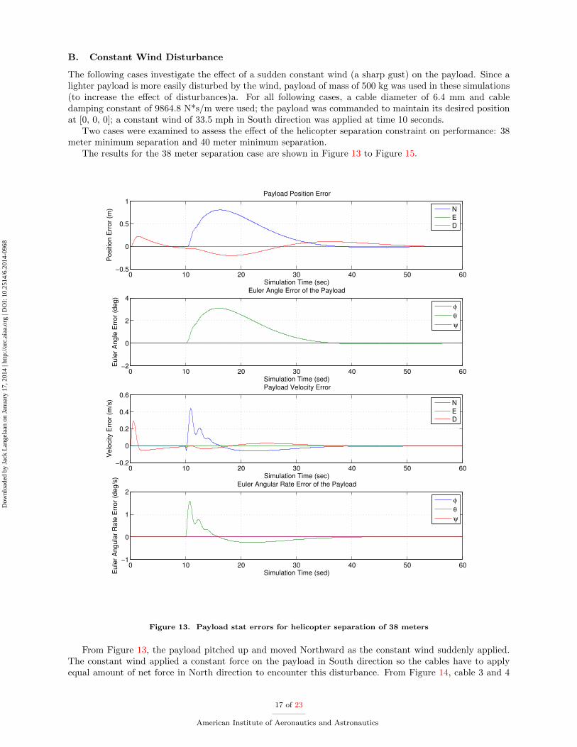
B. Constant Wind Disturbance

The following cases investigate the effect of a sudden constant wind (a sharp gust) on the payload. Since alighter payload is more easily disturbed by the wind, payload of mass of 500 kg was used in these simulations(to increase the effect of disturbances)a. For all following cases, a cable diameter of 6.4 mm and cabledamping constant of 9864.8 N*s/m were used; the payload was commanded to maintain its desired positionat [0, 0, 0]; a constant wind of 33.5 mph in South direction was applied at time 10 seconds.

Two cases were examined to assess the effect of the helicopter separation constraint on performance: 38meter minimum separation and 40 meter minimum separation.

The results for the 38 meter separation case are shown in Figure 13 to Figure 15.

0 10 20 30 40 50 60−0.5

0

0.5



Positio

n E

rror

(m)

N

E

D

0 10 20 30 40 50 60−2

0

2



Eule

r A

ngle

Err

or

(deg)

φ

θ

ψ

0 10 20 30 40 50 60−0.2

0

0.2

0.4

0.6Payload Velocity Error


Velo

city E

rror

(m/s

)

N

E

D

0 10 20 30 40 50 60−1

0

1

2Euler Angular Rate Error of the Payload

Simulation Time (sed)Eule

r A

ngula

r R

ate

Err

or

(deg/s

)

φ

θ

ψ

Figure 13. Payload stat errors for helicopter separation of 38 meters

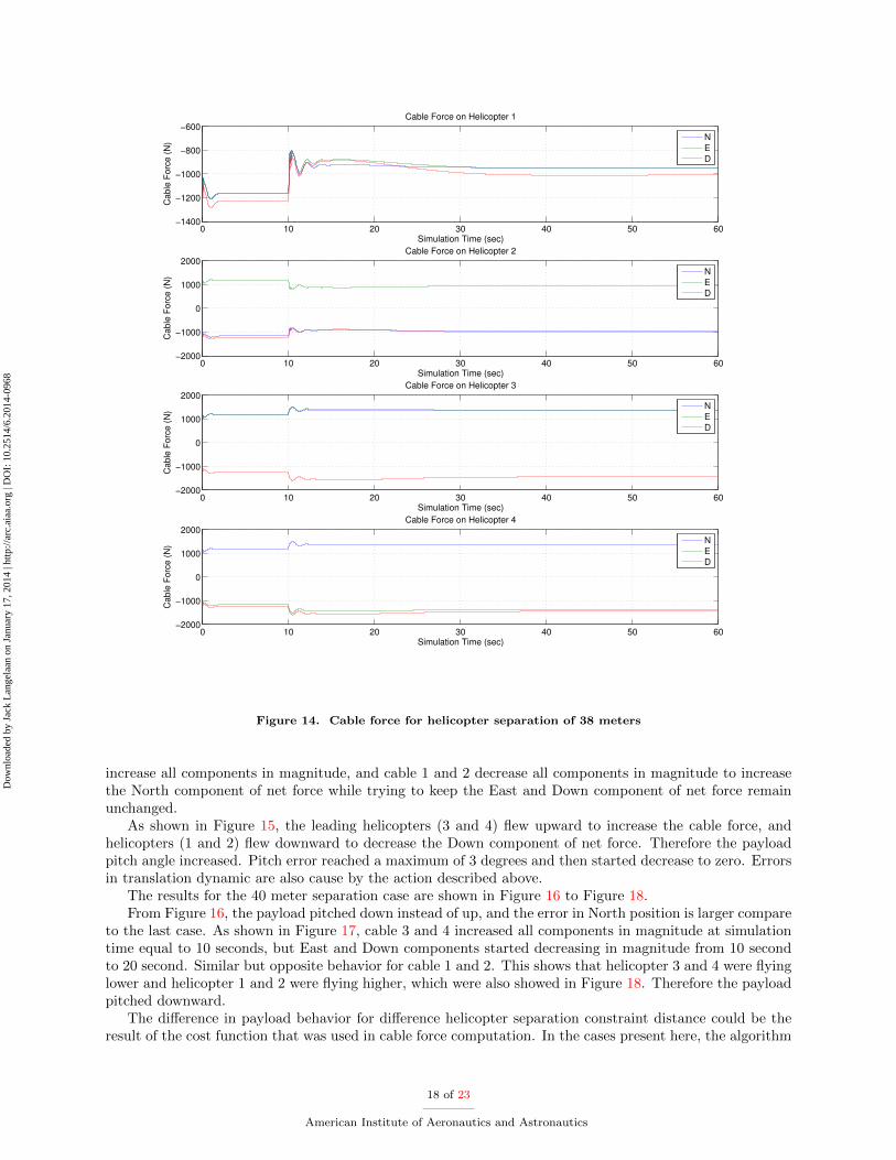
From Figure 13, the payload pitched up and moved Northward as the constant wind suddenly applied.The constant wind applied a constant force on the payload in South direction so the cables have to applyequal amount of net force in North direction to encounter this disturbance. From Figure 14, cable 3 and 4

17 of 23


Dow

nloa

ded

by J

ack

Lan

gela

an o

n Ja

nuar

y 17

, 201

4 | h

ttp://

arc.

aiaa

.org

| D

OI:

10.

2514

/6.2

014-

0968

0 10 20 30 40 50 60−1400

−1200

−1000

−800

−600Cable Force on Helicopter 1


Ca

ble

Fo

rce

(N

)

N

E

D

0 10 20 30 40 50 60−2000

−1000

0

1000

2000Cable Force on Helicopter 2


Ca

ble

Fo

rce

(N

)

N

E

D

0 10 20 30 40 50 60−2000

−1000

0

1000



Ca

ble

Fo

rce

(N

)

N

E

D

0 10 20 30 40 50 60−2000

−1000

0

1000



Ca

ble

Fo

rce

(N

)

N

E

D

Figure 14. Cable force for helicopter separation of 38 meters

increase all components in magnitude, and cable 1 and 2 decrease all components in magnitude to increasethe North component of net force while trying to keep the East and Down component of net force remainunchanged.

As shown in Figure 15, the leading helicopters (3 and 4) flew upward to increase the cable force, andhelicopters (1 and 2) flew downward to decrease the Down component of net force. Therefore the payloadpitch angle increased. Pitch error reached a maximum of 3 degrees and then started decrease to zero. Errorsin translation dynamic are also cause by the action described above.

The results for the 40 meter separation case are shown in Figure 16 to Figure 18.From Figure 16, the payload pitched down instead of up, and the error in North position is larger compare

to the last case. As shown in Figure 17, cable 3 and 4 increased all components in magnitude at simulationtime equal to 10 seconds, but East and Down components started decreasing in magnitude from 10 secondto 20 second. Similar but opposite behavior for cable 1 and 2. This shows that helicopter 3 and 4 were flyinglower and helicopter 1 and 2 were flying higher, which were also showed in Figure 18. Therefore the payloadpitched downward.

The difference in payload behavior for difference helicopter separation constraint distance could be theresult of the cost function that was used in cable force computation. In the cases present here, the algorithm

18 of 23


Dow

nloa

ded

by J

ack

Lan

gela

an o

n Ja

nuar

y 17

, 201

4 | h

ttp://

arc.

aiaa

.org

| D

OI:

10.

2514

/6.2

014-

0968

0 10 20 30 40 50 60−21.5

−21

−20.5

−20

−19.5

−19Helicopters Down position


He

licop

ters

Do

wn

positio

n

Helicopter 1

Helicopter 3

0 10 20 30 40 50 60−21.5

−21

−20.5

−20

−19.5



Helic

op

ters

Dow

n p

ositio

n

Helicopter 2

Helicopter 4

Figure 15. Helicopters Down direction position for 38 meter separation constraint

determined a set of cable force that will minimize the total cable force and satisfy the separation constraint.Based on the results from last two cases, we assume that there is one value of helicopter separation

constraint distance will result in smallest maximum payload pitch error due to the constant wind disturbance.Figure 19 is a plot that shows the relationship between payload maximum pitch angle error and helicopterseparation constraint distance with cost function that minimize the total cable force.

The the range of helicopter separation constraint distance for stable operation is from 37.65 to 41.55. Thisrange may change with different cost function for cable force computation. From Figure 19, the helicopterseparation constraint distance that results in smallest maximum payload pitch error is about 38.62 meters.Further studies will be conduct to investigate how is the optimal separation constraint distance relate topayload properties, cable properties, attachment point location, and the cost function used to compute thecable forces.

VI. Conclusion

This paper has presented a hierarchical approach to coordinated transport of a slung load by a teamof autonomous rotorcraft. The approach is based on the concept of object based task level control, whichabstracts control into several layers, with a high-level controller computing the desired forces to ensure that

19 of 23


Dow

nloa

ded

by J

ack

Lan

gela

an o

n Ja

nuar

y 17

, 201

4 | h

ttp://

arc.

aiaa

.org

| D

OI:

10.

2514

/6.2

014-

0968

0 10 20 30 40 50 60−2

−1

0



Po

sitio

n E

rro

r (m

)

N

E

D

0 10 20 30 40 50 60−10

−5

0



Eu

ler

An

gle

Err

or

(de

g)

φ

θ

ψ

0 10 20 30 40 50 60−0.5

0

0.5Payload Velocity Error


Ve

locity E

rro

r (m

/s)

N

E

D

0 10 20 30 40 50 60−2

−1

0

1Euler Angular Rate Error of the Payload

Simulation Time (sed)Eu

ler

An

gu

lar

Ra

te E

rro

r (d

eg

/s)

φ

θ

ψ

Figure 16. Payload stat errors for helicopter separation of 40 meters

the payload follows a desired trajectory. A lower level controller computes the required cable forces andinner loop controllers on board each helicopter ensure that these desired cable forces are maintained.

With three or more cable attachment points a payload can be controlled in six degrees of freedom, andthe resulting null space is used to ensure that other constraints (vehicle separation, payload controllabilityand disturbance rejection) are satisfied.

This paper has used a linear state feedback controller combined with a feed forward of desired accelerationas a payload trajectory following controller. A two step approach is used to compute cable forces: first, theleast norm solution ensures that net forces on the payload are satisfied; second, null space forces are computedso that constraints (here, vehicle separation) are satisfied.

Simulation results of payload transport using four helicopters and cables modeled as damped springsshow the utility of the approach. Payload state error remains small and disturbance rejection (response toa step gust) is good.

Acknowledgments

This research was partially funded by the Government under Agreement No. W911W6-11-2-0011. TheU.S Government is authorized to reproduce and distribute reprints notwithstanding any copyright notationthereon. The views and conclusions contained in this document are those of the authors and should not

20 of 23


Dow

nloa

ded

by J

ack

Lan

gela

an o

n Ja

nuar

y 17

, 201

4 | h

ttp://

arc.

aiaa

.org

| D

OI:

10.

2514

/6.2

014-

0968

0 10 20 30 40 50 60−1600

−1400

−1200

−1000

−800Cable Force on Helicopter 1


Ca

ble

Fo

rce

(N

)

N

E

D

0 10 20 30 40 50 60−2000

−1000

0

1000



Ca

ble

Fo

rce

(N

)

N

E

D

0 10 20 30 40 50 60−2000

−1000

0

1000



Ca

ble

Fo

rce

(N

)

N

E

D

0 10 20 30 40 50 60−2000

−1000

0

1000



Ca

ble

Fo

rce

(N

)

N

E

D

Figure 17. Cable force for helicopter separation of 40 meters

be interpreted as representing the official policies, either expressed or implied, of the U.S. Government.Theauthors also thank Thanan Yomchinda for providing the helicopter dynamic inversion control law used inthe simulations.

References

1Curtiss, H. C. and Warburton, F. W., “Stability and Control of the Twin-Lift Helicopter System,” Journal of theAmerican Helicopter Society, Vol. 30, No. 2, April 1985, pp. 14–23.

2Mittal, M., Prasad, J. V. R., and Schrage, D. P., “Comparison of Stability and Control Characteristics of Two Twin-LiftHelicopter Configurations,” Journal of Nonlinear Dynamics, Vol. 3, No. 3, 1992, pp. 199–223.

3Mittal, M. and Prasad, J. V. R., “Three-Dimensional Modeling and Control of a Twin-lift Helicopter System,” Journalof Guidance, Control and Dynamics, Vol. 16, No. 1, 1993, pp. 86–95.

4Maza, I., Kondak, K., and Bernard, M., “Multi-UAV Cooperation and Control for Load Transportation and Deployment,”Journal of Intelligent and Robotic Systems, Vol. 57, No. 1, 2010, pp. 417–449.

5Cicolani, L. S. and Kanning, G., “Equations of Motion of Slung-Load Systems, Including Multilift Systems,” Tech. Rep.TM-1038798, NASA, September 1992.

6Cicolani, L. S. and Kanning, G., “General equilibrium Characteristics of a Helicopter Dual-Lift System,” Tech. Rep.TP-2615, NASA, July 1986.

7Cicolani, L. S. and Kanning, G., “Equations of Motion of Slung Load Systems with Results for Dual Lift,” Tech. Rep.TM-102246, NASA, February 1990.

21 of 23


Dow

nloa

ded

by J

ack

Lan

gela

an o

n Ja

nuar

y 17

, 201

4 | h

ttp://

arc.

aiaa

.org

| D

OI:

10.

2514

/6.2

014-

0968

0 10 20 30 40 50 60−21

−20

−19

−18

−17



Helic

opte

rs D

ow

n p

ositio

n

Helicopter 1

Helicopter 3

0 10 20 30 40 50 60−21

−20

−19

−18

−17



Helic

opte

rs D

ow

n p

ositio

n

Helicopter 2

Helicopter 4

Figure 18. Helicopters Down direction position for 40 meter separation constraint

8Rodriquez, A. A. and Athans, M., “Multivariable Control of a Twin Lift Helicopter System using the LQG/LTR DesignMethodology,” American Controls Conference, June 1986, pp. 1325–1332.

9Menon, P. K., Prasad, J. V. R., and Schrage, D. P., “Nonlinear Control of a Twin-Lift Helicopter Configuration,” Journalof Guidance, Control and Dynamics, Vol. 14, No. 6, 1991, pp. 1287–1293.

10Prasad, J. V. R., Mittal, M., and Schrage, D. P., “Control of a Twin-Lift Helicopter System using Nonlinear StateFeedback,” Journal of the American Helicopter Society, Vol. 36, No. 4, 1991, pp. 57–65.

11Mittal, M., Prasad, J. V. R., and Schrage, D. P., “Nonlinear Adaptve Control of a Twin Lift Helicopter System,” IEEEControl Systems, Vol. 11, No. 3, 1991, pp. 39–45.

12Stevens, H. D., S., M. E., S.M., R., and Cannon, R., “Object-Based Task-Level Control: A Hierarchical Control Archi-tecture for Remote Operation of Space Robots,” Proceedings of the AIAA/NASA Conference on Intelligent Robotics in Field,Factory, Service, and Space, 1994.

13Song, Y., Horn, J. F., Li, Z., and Langelaan, J. W., “Modeling, Simulation and Non-linear Control of a RotorcraftMulti-lift System,” American Helicopter Society 69th Annual Forum, American Helicopter Society, Phoenix, AZ, May 21-232013.

14“K-MAX Performance and Specs,” http://www.kaman.com, Accessed: 20/11/2013.

22 of 23


Dow

nloa

ded

by J

ack

Lan

gela

an o

n Ja

nuar

y 17

, 201

4 | h

ttp://

arc.

aiaa

.org

| D

OI:

10.

2514

/6.2

014-

0968

http://www.kaman.com

37.5 38 38.5 39 39.5 40 40.5 41 41.5 420

2

4

6

8

10

12

Payload Pitch error vs. helicopter separation constraint distance

constraint distance (m)

ab

s(P

itch

err

or)

(d

eg

)

Figure 19. Payload pitch error vs. helicopter separation constraint

23 of 23


Dow

nloa

ded

by J

ack

Lan

gela

an o

n Ja

nuar

y 17

, 201

4 | h

ttp://

arc.

aiaa

.org

| D

OI:

10.

2514

/6.2

014-

0968

coordinated transport of a slung load by a team of

Documents