coordinated voltage control in active distribution network with … · coordinated voltage control...

Coordinated Voltage Control inActive Distribution Network with

On-load Tap Changer and SolarPV System Systems

Praveen Prakash SinghDepartment of Energy Technology, 2019

Master Project

ST

U

DE

NT R E P O R T

Department of Energy technologyAalborg University

Pontoppidanstræde 111, 9220 Aalborghttp://www.et.aau.dk

Title:Coordinated Voltage Control in ActiveDistribution Network with On-load TapChanger and Solar PV System

Theme:Master’s thesis

Project Period:Spring semester 2019

Project Group:EPSH

Participant(s):Praveen Prakash Singh

Supervisor(s):Jayakrishnan Radhakrishna PillaiSanjay Chaudhary

Copies: 1

Page Numbers: 40

Date of Completion:October 31, 2019

Abstract:

Decreasing cost and favorable policieshave resulted in increased penetration ofsolar PV within active distribution net-work. As the penetration of PV systemis likely to increase in future, utilizingthe reactive power capability to mitigateovervoltage is analyzed. In recent years,droop control of inverter based distributedenergy resources has emerged an as es-sential tool which will be investigated inthis work. The participation of PV systemin voltage regulation and its coordinationwith existing controllers such as OLTC isparamount to regulate the voltage withinthe specified limits. Developing controlstrategies which can be coordinated withthe existing control in a distributed man-ner is proposed in this work.

The content of this report is freely available, but publication (with reference) may only be pursued due toagreement with the author.

http://www.et.aau.dk

Contents

Preface vii

1 Introduction 11.1 General Background and Motivation . . . . . . . . . . . . . . . . . . . . . . . . 11.2 Problem Statement . . . . . . . . . . . . . . . . . . . . . . . . . . . . . . . . . . 31.3 Objectives . . . . . . . . . . . . . . . . . . . . . . . . . . . . . . . . . . . . . . . 31.4 Limitation . . . . . . . . . . . . . . . . . . . . . . . . . . . . . . . . . . . . . . . 4

2 State of Art 52.1 Overview of Distribution system . . . . . . . . . . . . . . . . . . . . . . . . . . 52.2 Impact of DER on Voltage Drop in Distribution System . . . . . . . . . . . . . 62.3 Voltage Control using On-load Tap Changer (OLTC) . . . . . . . . . . . . . . 82.4 Voltage Control using DER Interfaced with Inverter . . . . . . . . . . . . . . 92.5 Solar Photovoltaic System . . . . . . . . . . . . . . . . . . . . . . . . . . . . . . 112.6 Grid Codes . . . . . . . . . . . . . . . . . . . . . . . . . . . . . . . . . . . . . . . 12

3 Steady State Analysis of Medium Voltage Distribution Network 133.1 Modelling of MV Grid . . . . . . . . . . . . . . . . . . . . . . . . . . . . . . . . 133.2 Sensitivity Analysis of Grid . . . . . . . . . . . . . . . . . . . . . . . . . . . . . 153.3 Analysis of DER Indices . . . . . . . . . . . . . . . . . . . . . . . . . . . . . . . 173.4 Chapter Summary . . . . . . . . . . . . . . . . . . . . . . . . . . . . . . . . . . 18

4 Effect of Solar PV and OLTC on Voltage Control 194.1 Generation and load profiles . . . . . . . . . . . . . . . . . . . . . . . . . . . . 194.2 Operation of OLTC control . . . . . . . . . . . . . . . . . . . . . . . . . . . . . 204.3 Q-V Droop Control of PV inverter . . . . . . . . . . . . . . . . . . . . . . . . . 234.4 Chapter summary . . . . . . . . . . . . . . . . . . . . . . . . . . . . . . . . . . . 25

5 Voltage control using OLTC and Droop Control 275.1 Uncoordinated control of OLTC and Q-V control . . . . . . . . . . . . . . . . 275.2 Coordinated control of OLTC and PV droop control . . . . . . . . . . . . . . . 305.3 Chapter Summary . . . . . . . . . . . . . . . . . . . . . . . . . . . . . . . . . . 33

6 Conclusions and Future Work 356.1 Conclusions . . . . . . . . . . . . . . . . . . . . . . . . . . . . . . . . . . . . . . 356.2 Future Work . . . . . . . . . . . . . . . . . . . . . . . . . . . . . . . . . . . . . . 35

v

vi Contents

Bibliography 37

Preface

This project is about voltage control in active distribution network in the presence of SolarPV system. A coordinated control approach is required to operate the active distributionnetwork within permisisble voltage range.

I would like thank my Associate Professor Jayakrishnan Radhakrishna Pillai for givingme the chance to make a research in Voltage control using OLTC and Q-V droop controlwhich is very interesting topic and for their extensive support during this semester. Iwould like also thanks Associate Professor Sanjay Chaudhary for his advises. Finally, Iwould like to thank my father and brothers for supporting me and understand my stressthis period.

Aalborg University, October 31, 2019

Praveen Parakash Singh<[email protected]>

vii

Chapter 1

Introduction

A brief review of the relevant topics in transmuting energy sector is presented in this chapter.The general motivation and background manifest the ambitions of escalating the integration ofdistributed energy resources (DER’s) in the active distribution network, and the key issues areaddressed. Consequently, the problem statement bounded by a few limitations is described and themethodology used to solve the problems are presented in further sections. Finally, the outline of thethesis is summarized and contextualized.

1.1 General Background and Motivation

Global renewable energy deployment has been on the forefront in Europe over two decadesto curtail the rise in temperature "well below 2◦ C" concerning pre-industrial levels. Thefastest growing technology in renewable power generation until 2017 is solar PV (98 GW)than other renewable peers such as large hydro (19 GW) and wind (52 GW) [1]. The costreduction of critical technologies such as PV, wind and other renewable sources accompa-nied by improvised end-user technology, the EU is currently on course for accomplishingthe objective of 20% renewable share by 2020 and attain global leadership by 2030 with ashare of 27% which can be increased to 34% taking energy efficiency into account (see Fig.1.1) [2].

Figure 1.1: Renewable energy options for 2030 target [2]

1

2 Chapter 1. Introduction

Figure 1.2: Expected future trend of Danish installed generation [3]

The Danish power system constitutes the highest share of variable renewable energy inwhich wind power has a share of 44% while PV production contribution is only 2% ofthe total Danish electricity consumption in 2017 (see Fig. 1.2) [3]. It can also be inferredthat the electricity demand is lower than the generation which might increase in the futureincreasing the burden on the grid which may adversely affect the performance and oper-ation of the grid. Escalating renewable power production have resulted in growth of thedistributed energy resources (DER) in the distribution system. The intermittent nature ofvariable renewable energy resources such as solar and wind power production along withthe arbitrarily changing load demand necessitates the increase in flexibility of the grid.The mismatch between the generation and demand i.e. the residual load management isa critical aspect for determining the power system flexibility needs which can be achievedby increasing interconnections, power-to-X, demand side response and storage. Flexiblegeneration may also be used in case of high demand. [4].

Voltage control issue in presence of DER in the distribution grid has been a subject ofinterest for many years and various approaches have been suggested by many researchers.A summary of steady-state and dynamic effect of solar photovoltaic penetration in the dis-tribution network given in [5], addressed issues such as malfunctioning of voltage regulat-ing devices and/or OLTC transformer, overloading of distribution feeder, voltage flickerand unbalance among others. In [6], investigation of distribution system due to reversalof power flow resulting in notable adjustment in power factor may alter the performanceof transformer in regulating the voltage of the system. The technical solutions consideringvoltage and thermal limits to enhance the distribution system operator (DSO) access toflexibility as proposed in [7] are advanced control of HV/MV transformer, DSO storage,on-load tap changer for MV/LV transformers, network reinforcement and reconfigurationto enhance PV hosting capacity. In [6], the impact on voltage regulation using OLTC trans-formers with and without LDC in medium voltage feeders with distributed generation ispresented. General Electrics (GE) in [8] illustrated the control of power electronics insidesmart inverter for voltage support investigating the constant power factor mode and Volt/-VAR control function. A coordinated control of battery energy storage system (BESS) with

1.2. Problem Statement 3

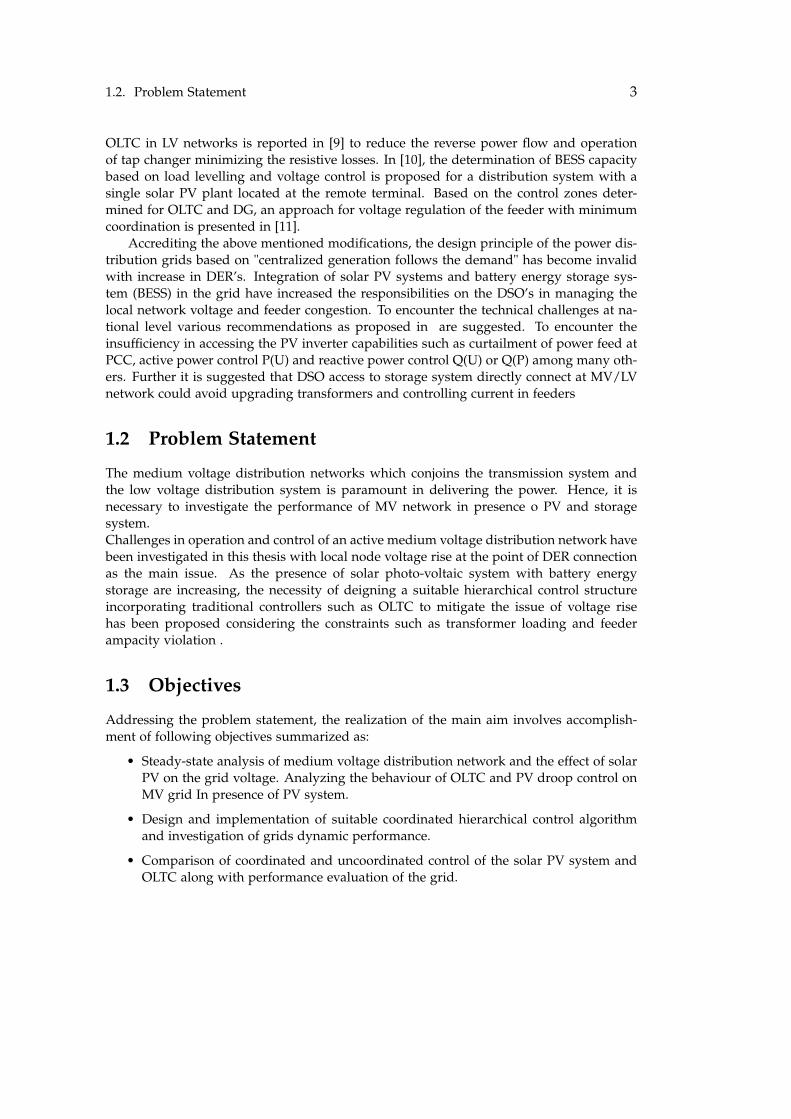
OLTC in LV networks is reported in [9] to reduce the reverse power flow and operationof tap changer minimizing the resistive losses. In [10], the determination of BESS capacitybased on load levelling and voltage control is proposed for a distribution system with asingle solar PV plant located at the remote terminal. Based on the control zones deter-mined for OLTC and DG, an approach for voltage regulation of the feeder with minimumcoordination is presented in [11].

Accrediting the above mentioned modifications, the design principle of the power dis-tribution grids based on "centralized generation follows the demand" has become invalidwith increase in DER’s. Integration of solar PV systems and battery energy storage sys-tem (BESS) in the grid have increased the responsibilities on the DSO’s in managing thelocal network voltage and feeder congestion. To encounter the technical challenges at na-tional level various recommendations as proposed in are suggested. To encounter theinsufficiency in accessing the PV inverter capabilities such as curtailment of power feed atPCC, active power control P(U) and reactive power control Q(U) or Q(P) among many oth-ers. Further it is suggested that DSO access to storage system directly connect at MV/LVnetwork could avoid upgrading transformers and controlling current in feeders

1.2 Problem Statement

The medium voltage distribution networks which conjoins the transmission system andthe low voltage distribution system is paramount in delivering the power. Hence, it isnecessary to investigate the performance of MV network in presence o PV and storagesystem.Challenges in operation and control of an active medium voltage distribution network havebeen investigated in this thesis with local node voltage rise at the point of DER connectionas the main issue. As the presence of solar photo-voltaic system with battery energystorage are increasing, the necessity of deigning a suitable hierarchical control structureincorporating traditional controllers such as OLTC to mitigate the issue of voltage risehas been proposed considering the constraints such as transformer loading and feederampacity violation .

1.3 Objectives

Addressing the problem statement, the realization of the main aim involves accomplish-ment of following objectives summarized as:

• Steady-state analysis of medium voltage distribution network and the effect of solarPV on the grid voltage. Analyzing the behaviour of OLTC and PV droop control onMV grid In presence of PV system.

• Design and implementation of suitable coordinated hierarchical control algorithmand investigation of grids dynamic performance.

• Comparison of coordinated and uncoordinated control of the solar PV system andOLTC along with performance evaluation of the grid.

4 Chapter 1. Introduction

1.4 Limitation

There are several limitation which are assumed which are enlisted below

• The network is assumed to be balanced.

• The solar PV system is considered as static generator.

• The transient and dynamic behaviour of OLTC and PV control has not been consid-ered.

•

Chapter 2

State of Art

In this chapter, a literature review of the relevant topics related to the voltage drop along the feederand its compensation technique using on-load tap changer along with line drop compensation tech-nique is discussed. An overview of solar PV and battery energy storage system is presented alongwith the control techniques used for voltage regulation. A review of the grid codes involved in thisproject are also analyzed.

2.1 Overview of Distribution system

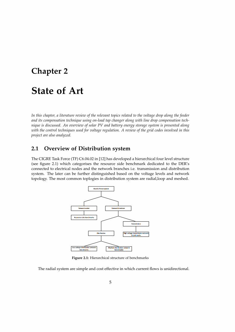
The CIGRE Task Force (TF) C6.04.02 in [12] has developed a hierarchical four level structure(see figure 2.1) which categorises the resource side benchmark dedicated to the DER’sconnected to electrical nodes and the network branches i.e. transmission and distributionsystem. The later can be further distinguished based on the voltage levels and networktopology. The most common toplogies in distribution system are radial,loop and meshed.

Figure 2.1: Hierarchical structure of benchmarks

The radial system are simple and cost effective in which current flows is unidirectional.

5

6 Chapter 2. State of Art

In case of loop system two radially operating feeders are connected at the remote terminalto form a ring like structure and the flow of current is bidirectional. The meshed systemconstitutes a large interconnection of feeders having high complexity and reliability [13].

The Distribution feeder is generally expressed as lumped π-model [14][15] as shownin figure x which constitutes series resistance (RL) and inductance (XL) and the shuntcomponent represents the susceptance (B) of the line. The voltage and current at both(sending and receiving) end can be related by :∣∣∣∣Us

Is

∣∣∣∣ =∣∣∣∣∣ 1 + 1

2ZYl2 ZlYl(1 + ZYl2

4 ) 1 + 12ZYl2

∣∣∣∣∣∣∣∣∣ Vr−Ir

∣∣∣∣ (2.1)

Figure 2.2: Distribution feeder π-model

Expressing the impedance of line as admittance (Y = Z−1), the power flow equationfor between the sending and receiving end can be given as [16]:

SPSL = V2P(GL + jBL + Bsh/2)−VPVS(GL + jBL)e− j(θP − θS) (2.2)

This non-linear power flow equation is solved using iterative method such as Gauss-Seideland Newtwon-Rapshon which will be considered in the next chapter.

2.2 Impact of DER on Voltage Drop in Distribution System

The voltage drop caused due to the flow of current can be analyzed using a simple singleline diagram (see figure 2.3). Let us consider a simple feeder having impedance Z(R + jX)through which power flows from sending end (US) to receiving end voltage (UR) to supplythe load (PL + jQL).The complex line current can be expressed as the ratio of receiving endapparent power and voltage [17]:

I =S∗RU∗R

=PR − jQR

U∗R(2.3)

where PR + jQR = (PL − PG) + j(QL − QG). Initially it is assumed that no contributionis made from the PV. Also, the voltage drop along the distribution feeder i.e. differencebetween the sending and receiving end voltage can be given as [18]:

∆V =| US | − | UR |= I.Z (2.4)

2.2. Impact of DER on Voltage Drop in Distribution System 7

Figure 2.3: Single line diagram of a feeder connected with PV and load

The phasor diagram (see figure 2.4) assumes that the current lags the voltage (i.e.X>R)by an angle φ and no contribution is made by the PV. The shunt capacitance is also assumedto be negligible. The current vector can be resolved into active and reactive componentswhich can be substituted in eq.((2.2) to give an approximated voltage drop as [18], [19]:

∆U = IRcosφ + IXsinφ (2.5)

Considering O as the center, if a circle is drawn of radius US, the difference betweenthe estimated and actual voltage drop can be calculated (see figure 2.4). This error can beexpressed as [19]:

error = US −√

U2S − (IXcosφ− IRsinφ)2 (2.6)

Figure 2.4: Phasor diagram of a feeder connected with PV and load

The actual voltage drop along a feeder can be obtained by adding equations (2.5) and(2.6) (see eq. (2.1)). It can be inferred that the voltage drop depends on the R/X ratio,load current and phase angle between load current and receiving end voltage. When PV


is taken into account, the voltage drop change in current which can be expressed as:

I =(PR − PPV)− j(QR −QPV)

U∗R(2.7)

where PPV and QPV is real and reactive power generated by the PV. The sign conventionof reactive power associated to the converter may change as the inverter control actionstake place. The current injected in the grid depends on the receiving end complex voltageand apparent power. When the DG is inserted in the network the voltage .

2.3 Voltage Control using On-load Tap Changer (OLTC)

To ensure operating voltage is within the limits, voltage control in medium voltage net-work is achieved using on-load tap changers (OLTC) to regulate the voltage at the remoteterminal [20]. The principle of operation of OLTC, voltage regulators and auto-transformerare similar. Figure 2.5 represents the schematic of OLTC transformer along with its equiv-alent circuit. The primary and secondary side are denoted by the notations p and s, whereU, I, Z and n corresponds to voltage, current, impedance and turn ratio of the transformerrespectively [17].The OLTC mechanism may be either on high voltage side or low voltageside. Usually, the tap changer are provided towards high voltage side as the current islow which makes it easier for switching the current following the concept of "make beforebreak". Also, the availability of large number of turns help in achieving regulation withhigher precision [21].

Figure 2.5: Schematic representation of OLTC with equivalent circuit [17]

The complex voltage flowing through the transformer can be expressed as in eq.(2.2)including the complex tap of the transformer as:

SPST = V2P t2(GL + jBL + Bsh)−VPVS(GL + jBL)te− j(θP − θS + φt) (2.8)

Figure 2.6 given in [20], [22] represents the basic control structure for regulating the busvoltage using OLTC with LDC (Line drop compensation). The bank current and bus ter-

2.4. Voltage Control using DER Interfaced with Inverter 9

minal voltage information is accessed using C.T. and P.T. The voltage drop is estimated byusing the bank current, resistance and reactance from the transformer to the point wherevoltage is being regulated. The reference voltage set point is the midpoint of higher andlower voltage limits and is also know as "voltage band center".The OLTC can also be performed without LDC. In such as case, the bank current is notrequired and the difference between bus voltage and reference voltage is eliminated bychanging the tap position [6]. The voltage relationships can be written as :

Umax ≥ Usig ≥ Umin and Usig = Uact −Ure f =

{positive, for overvoltagenegative, for undervoltage

(2.9)

Figure 2.6: Control of voltage using on-load tap changing [20], [22]

In addition to this, an intentional time delay is provided prior to tap changing actionwhen the voltage is "out of band" to avoid unnecessary changes during stable operation ofthe grid. Position 1 and 3 corresponds to counter start during which control mechanismis initiated. If the voltage is out of bandwidth for certain time delay, transformers tapposition is altered otherwise counter stop is executed to stop the control action as shownby position 2.

In case for OLTC with LDC setting, the resistance and reactance setting can be obtainedas [6]:

Req =NCTNPT

RL and Xeq =NCTNPT

XL (2.10)

where = (NCT) and (NPT) are the turns ratio of C.T. and P.T. The load resistance (RL) andreactance (XL) represents the and feeder impedance connected to the transformer.

2.4 Voltage Control using DER Interfaced with Inverter

Taking into account the dependency on power production, the DER’s interfaced with thegrid at PCC can be enlisted in four categories: direct machine coupling, full power elec-tronics, partial power electronics and modular or distributed power electronics interface


[23]. The most efficient is the direct machine coupling as it doesn’t require any interme-diate stage. For power generation with power electronic converter as intermediate stage,the type of category it belongs to depends on the size and type of power generation tech-nology. The control strategies adopted for grid connected PV inverters can be broadlyclassified into two categories [24] (see figure 2.7).

Figure 2.7: Classification of Distributed PV control

• Autonomous/local Control

Grid connected power electronics can be utilized to enhance flexible control for the stablesystem operation. This type control actions are generally fast as it involved controllinggate pulses of the power electronic switches which are operated at high frequencies. Theinverter based DER’s distributed throughout the network can be locally/internally con-trolled by three methods as suggested in [24]:(i) V/f Control: In V/f control, the DER is modelled as a voltage source with a low se-ries impedance. The inverter operates in grid-forming mode to maintain the voltage andfrequency at desired set points. The active and reactive power exchanged with the grid de-pends on the system loading conditions. The local grid voltage and frequency are sensedand controlled actions are performed in closed loop manner. [24][25].(ii) P-Q Control: In this control mode, the inverter is operated in greed-feeding modei.e. a current source in parallel to a high impedance. The control actions are performedby obtaining the decoupled active and reactive power are controlled independently withrespective to desired set points. Most of the DER fall under this category [25].(iii)Droop Control: The droop control technique is a grid-supporting function which isamong the popular choice of control for distributed power converters as they overcomethe problem of load sharing when operating in parallel within a grid. They can be eitheroperated separately or in combination with other two methods [26].

2.5. Solar Photovoltaic System 11

• System-level Control

The control strategies applied at system level fall under this category. Various equipment’sare connected to distribution network which are used to operate the grid satisfactorily.This level of control can be broadly classified into following three categorize [24]:(i)Master-Slave Control: In this type of control strategy, one of the converter is operated inV/f control mode to maintain the voltage and provide reference current to the other DERenabled as slaves. These converters are operated in P-Q mode enabling efficient decoupledactive and reactive power control. The master of the slave can be determined in variousways as reported in [27].(ii)Hierarchical Control: In this type of control, the command signals are generated ac-cording to network requirements at a central location (such as substations), which latercommunicated to the rest of inverters within the grid for executing necessary changes.They are also referred as centralized/ concentrated control. The major drawback asso-ciated with this method is if the central controller (master) fails to response, the controlactions required won’t be executed . These controls require common synchronisation sig-nal and current sharing module which determines the reference current for each modulewith respect to load current [24], [27].

(iii)Peer-to-Peer Control: This type of control is also known as distributed controlwhich has the properties of both autonomous control and centralized control. The controlactions are initiated locally to control the bus voltage locally. However, control actions arealso communicated through central level controllers when local control cannot regulate thebus voltage. When the local control is not sufficient, centralized control actions take place[28].

2.5 Solar Photovoltaic System

The solar power can be harnessed in many ways such as directly converting the solarirradiance into electricity using solar panel converting the energy from photons, hybridplants, concentrated solar power plants (CSP),etc [29]. In this thesis the focus is mainlyon the solar photovoltaic systems. The semiconductor cells also known as wafers areused in solar panel to produce photocurrent when exposed to solar irradiation.The powerproduced by the panel is in DC (or kW) which can be expressed in relation with solarirradiation as:.

P = η.A.S.FF (2.11)

where η is the efficiency of solar panel which is generally ranges from 15% to 17%, FFis the fill factor which determines the quality of cell, S is the solar irradiation (in W/m2)and A is the area of the collector. The PV panel are generally interface with inverter forconverting the power from DC to AC.


2.6 Grid Codes

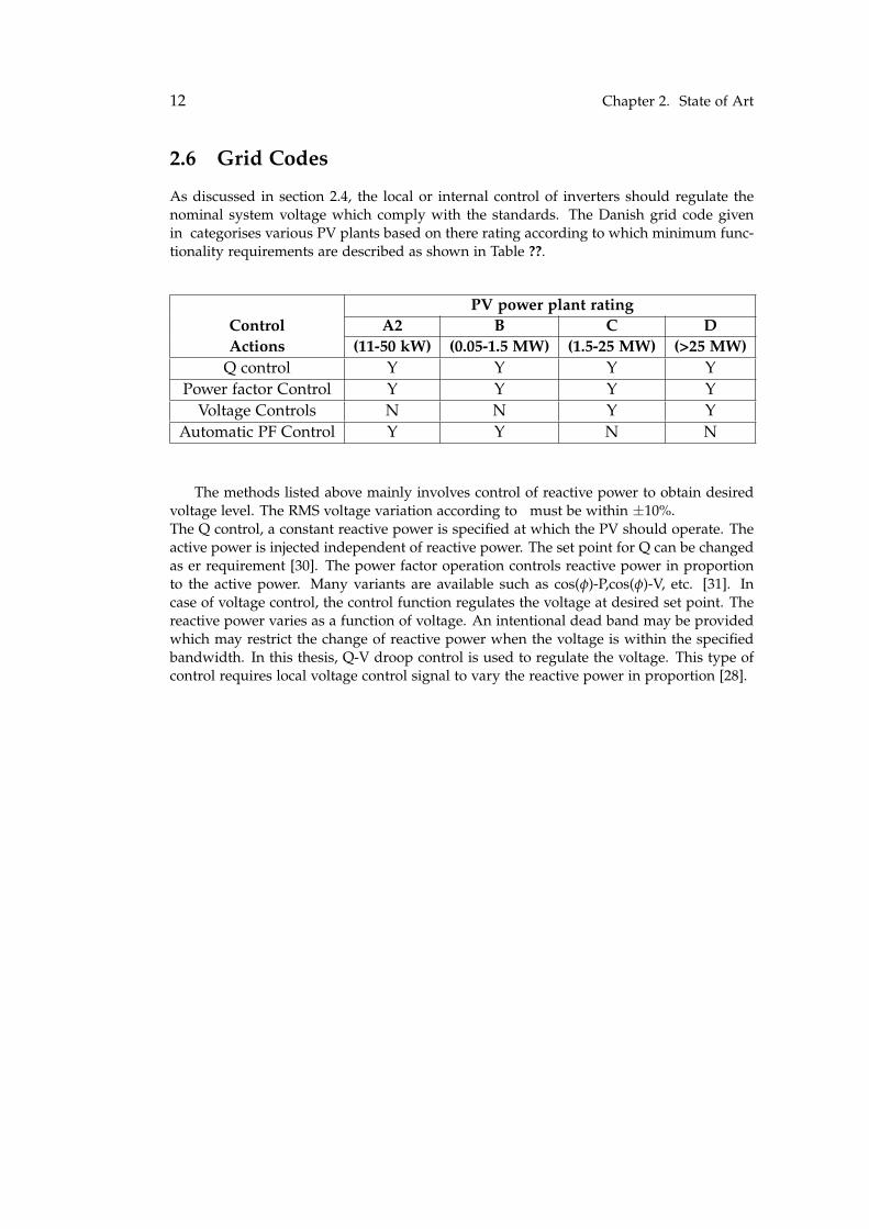
As discussed in section 2.4, the local or internal control of inverters should regulate thenominal system voltage which comply with the standards. The Danish grid code givenin categorises various PV plants based on there rating according to which minimum func-tionality requirements are described as shown in Table ??.

PV power plant ratingControl A2 B C DActions (11-50 kW) (0.05-1.5 MW) (1.5-25 MW) (>25 MW)

Q control Y Y Y YPower factor Control Y Y Y Y

Voltage Controls N N Y YAutomatic PF Control Y Y N N

The methods listed above mainly involves control of reactive power to obtain desiredvoltage level. The RMS voltage variation according to must be within ±10%.The Q control, a constant reactive power is specified at which the PV should operate. Theactive power is injected independent of reactive power. The set point for Q can be changedas er requirement [30]. The power factor operation controls reactive power in proportionto the active power. Many variants are available such as cos(φ)-P,cos(φ)-V, etc. [31]. Incase of voltage control, the control function regulates the voltage at desired set point. Thereactive power varies as a function of voltage. An intentional dead band may be providedwhich may restrict the change of reactive power when the voltage is within the specifiedbandwidth. In this thesis, Q-V droop control is used to regulate the voltage. This type ofcontrol requires local voltage control signal to vary the reactive power in proportion [28].

Chapter 3

Steady State Analysis of MediumVoltage Distribution Network

3.1 Modelling of MV Grid

A practical 20 kV MV network from a rural part of southern Germany which is derived bythe CIGRE task force [12] for the European configuration is considered (see Fig. 3.1 ). Thethree phase feeders are considered to be balanced and the topology of the network can bechanged by connecting the feeders using switches S1, S2 and S3 (see section 2.1).

Figure 3.1: 20 kV CIGRE MV benchmark network

13

14 Chapter 3. Steady State Analysis of Medium Voltage Distribution Network

The 14-bus system consists of two feeders which are energised using an external gridconnected at bus-0. The R/X ratio is 0.1 with short circuit capacity of 5000 MVA whichsuggests the network is very strong. Feeder-1 is mostly consists of underground cables(UC) while feeder-2 comprise of overhead lines (OHL). These distribution feeders alsodiffer in their lengths resulting in different impedance between the nodes. The HV/MVtransformers are of equal rating (25 MVA 110/20 kV) which are considered without tapchange mechanism initially. There are two different kind of load present in the grid:residential and industrial. The loads are highest near the transformer on both the feeders.The related data obtained from [12] for modelling is given in Appendix A. The geometricalparameters for the conductors have not been taken into account. The performance of thegrid is analyzed with all the switches (S1, S2 and S3) open i.e radial configuration.

In DigSilent PowerFactory, the load flow analysis is carried out using Newton-Raphsonmethod. Feeder-1 and feeder-2 can be analyzed individually as all the switches and bothare connected to each other via external grid which is considered as a slack bus in this case.All other remaining buses are considered as PQ bus or load bus as no generator is presentat any bus present in the system. The Jacobian matrix relating the power mismatches tovoltage (magnitude and phase angle) corrections are solved for each iteration for feedercan be expressed as [32]: [

∆P∆Q

]=

[JPθ = ∂P

∂θ JPV = ∂P∂V

JQθ = ∂Q∂θ JQV = ∂Q

∂θV

] [∆θ∆V

](3.1)

where,

JPθ =

{∂Piθi = −Qi | V2

i | Bii∂Pi∂θ j = − | ViVjYijsin(θij − θj − θi)

(3.2)

JPV =

∂PiVi

=Pi+|V2

i |GiiVi

∂Pi∂θ j =| ViVjYijcos(θij + θj − θi)

(3.3)

JQθ =

{∂Qiθi = Pi | V2

i | Gii∂Qi∂θ j = − | ViVjYijcos(θij − θj − θi)

(3.4)

JQV =

∂QiVi

=Qi+|V2

i |BiiVi

∂Pi∂θ j =| ViVjYijcos(θij + θj − θi)

(3.5)

The diagonal and off diagonal elements of eq. (3.23.5) represent the change in real andreactive power flow injection at a particular node with respect to voltage magnitude andangle at each bus [14]. The nodal power injections are the sum of all the line flow connectedto it as given in eq. (2.102.8). Figure (3.2) represents the voltage magnitude of each bus inthe system. As the voltage magnitude of feeder-2 is close to 1 .p.u. its not considered in thiswork. It can be inferred in most of the distribution lines of feeder-1 the voltage magnitudedifference is quite low due to which voltage drop along all the feeders are quite low. Line1-2 and line 2-3 which carry the total current delivering to bus-4, bus-8 and to the loadconnected at bus-3 have significantly higher voltage drop. Comparatively, voltage drop inLine 2-3 is higher as its length is greater than line 1-2 (see Appendix ??) The voltage drop

3.2. Sensitivity Analysis of Grid 15

across Line 1-2 is lower as compared to Line 2-3. This is because of absence of load at bus-2. The bus voltage deviation is minimal near the source as the R/X ratio of transformeris very less compared to the distribution feeder [28]. The voltage drop the rest of linesis quite low as the apparent power rating loads present within the system from bus-4 tobus-11. Hence deviation of voltage with respect to its sending voltage is quite low.

Figure 3.2: Voltage drop across lines in feeder-1

3.2 Sensitivity Analysis of Grid

The sensitivity coefficients often are used for associating the static scenario to the grid tocontrol logic using linearized power flow. The Jacobian sub-matrices can be utilized toformulate the voltage sensitivity coefficients. For instance to derive the Q-V sensitivityrelation, we set ∆P=0 and rewrite eq. (3.1) as: )[33][14]:

∆V∆Q

= (JPV − JQθ JPθ−1 JPV)−1 (3.6)

Similarly, the expression can be obtained for V-P sensitivity can be obtained by setting∆Q = 0:

∆V∆P

= (JPV − JPθ JQθ−1 JQV)−1 (3.7)

It can be seen that in every sensitivity relation, all the Jacobian sub-matrices are present.The diagonal elements of eq. (3.6 and3.7) represent the change in real and reactive powerflow injection at a particular node will cause deviation of its nodal voltage. Similarly, vari-ation of voltage due to power injection at another node can be calculated. [14]. AppendixA enlists the the sensitivity relations of each bus with respect to each other in matrix form(for both dV/dQ and dV/dP) for feeder-1. The sensitivity of feeder-2 is quite low due towhich it is not considered in this project. It can be observed that the tail end of the feederhas very high sensitivities as compared to the nodes located near the transformer. Highervalue of sensitivity indicated the consumer located at the feeder end has greater flexibil-ity for power production. It should also be noted that the sensitivity relations of bus-7to bus-11 are quite similar and very high compared to rest of the network. Bus-8 alsohave sensitivity similar to bus-9, however the difference with bus-7 is comparable. Bus-4


to bus-6 have similar sensitivity but is quite low as compared to bus 7-11. Bus-3 belongsto separate category as its sensitivity are different from the rest of the nodes within thefeeder. The sensitivity of bus-1 and bus-2 are very low suggesting lack of flexibility for theconsumers located near the transformer. Similar behaviour is observed for V-Q sensitivityhowever, the dependence of voltage deviation on reactive power change is higher thandV/dP sensitivity. This is because the reactance of the feeder is quite higher than the resis-tance. From this observation, feeder-1 is categorised in three different zones as shown infigure x. As the sensitivities of bus-3 and bus-8 are different from the rest of the network,they are excluded out of all the zones. Another reason for excluding these buses are thenumber of feeder connections at these buses are higher due to which effect of variation ofvoltage will be different.

Figure 3.3: Different zones in the feeder based on sensitivity

The total voltage magnitude variation at any node (say bus-i) cause by the active powerinjection of PV at any number of given bus will be given by:

∆Vi =∆Vi∆Pi

+N

∑j=1, 6=i

∆Vi∆Pj

(3.8)

where N is the number of buses present in the feeder. When the number of solar PVincrease in the grid, the magnitude rise will also increase. If the PV is injecting reactivepower, dV/dQ sensitivity should also be taken account. A comparative analysis is requiredto analyze how much change in voltage is observed when the presence of PV increases in

3.3. Analysis of DER Indices 17

the feeder. Hence an investigation regarding number of PV and their effect on bus voltage11 is necessary which will be performed in the next section.

3.3 Analysis of DER Indices

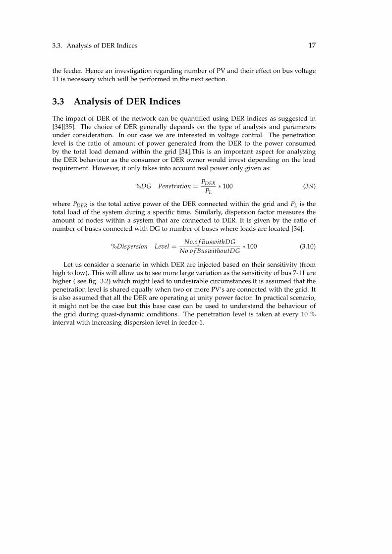
The impact of DER of the network can be quantified using DER indices as suggested in[34][35]. The choice of DER generally depends on the type of analysis and parametersunder consideration. In our case we are interested in voltage control. The penetrationlevel is the ratio of amount of power generated from the DER to the power consumedby the total load demand within the grid [34].This is an important aspect for analyzingthe DER behaviour as the consumer or DER owner would invest depending on the loadrequirement. However, it only takes into account real power only given as:

%DG Penetration =PDER

PL∗ 100 (3.9)

where PDER is the total active power of the DER connected within the grid and PL is thetotal load of the system during a specific time. Similarly, dispersion factor measures theamount of nodes within a system that are connected to DER. It is given by the ratio ofnumber of buses connected with DG to number of buses where loads are located [34].

%Dispersion Level =No.o f BuswithDG

No.o f BuswithoutDG∗ 100 (3.10)

Let us consider a scenario in which DER are injected based on their sensitivity (fromhigh to low). This will allow us to see more large variation as the sensitivity of bus 7-11 arehigher ( see fig. 3.2) which might lead to undesirable circumstances.It is assumed that thepenetration level is shared equally when two or more PV’s are connected with the grid. Itis also assumed that all the DER are operating at unity power factor. In practical scenario,it might not be the case but this base case can be used to understand the behaviour ofthe grid during quasi-dynamic conditions. The penetration level is taken at every 10 %interval with increasing dispersion level in feeder-1.


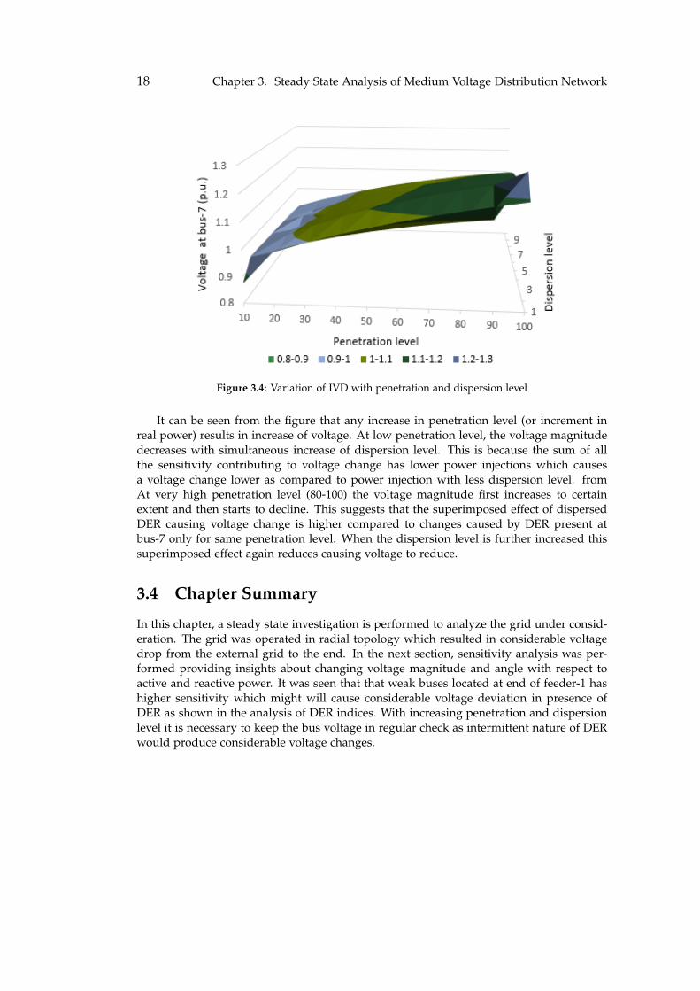
Figure 3.4: Variation of IVD with penetration and dispersion level

It can be seen from the figure that any increase in penetration level (or increment inreal power) results in increase of voltage. At low penetration level, the voltage magnitudedecreases with simultaneous increase of dispersion level. This is because the sum of allthe sensitivity contributing to voltage change has lower power injections which causesa voltage change lower as compared to power injection with less dispersion level. fromAt very high penetration level (80-100) the voltage magnitude first increases to certainextent and then starts to decline. This suggests that the superimposed effect of dispersedDER causing voltage change is higher compared to changes caused by DER present atbus-7 only for same penetration level. When the dispersion level is further increased thissuperimposed effect again reduces causing voltage to reduce.

3.4 Chapter Summary

In this chapter, a steady state investigation is performed to analyze the grid under consid-eration. The grid was operated in radial topology which resulted in considerable voltagedrop from the external grid to the end. In the next section, sensitivity analysis was per-formed providing insights about changing voltage magnitude and angle with respect toactive and reactive power. It was seen that that weak buses located at end of feeder-1 hashigher sensitivity which might will cause considerable voltage deviation in presence ofDER as shown in the analysis of DER indices. With increasing penetration and dispersionlevel it is necessary to keep the bus voltage in regular check as intermittent nature of DERwould produce considerable voltage changes.

Chapter 4

Effect of Solar PV and OLTC on Volt-age Control

4.1 Generation and load profiles

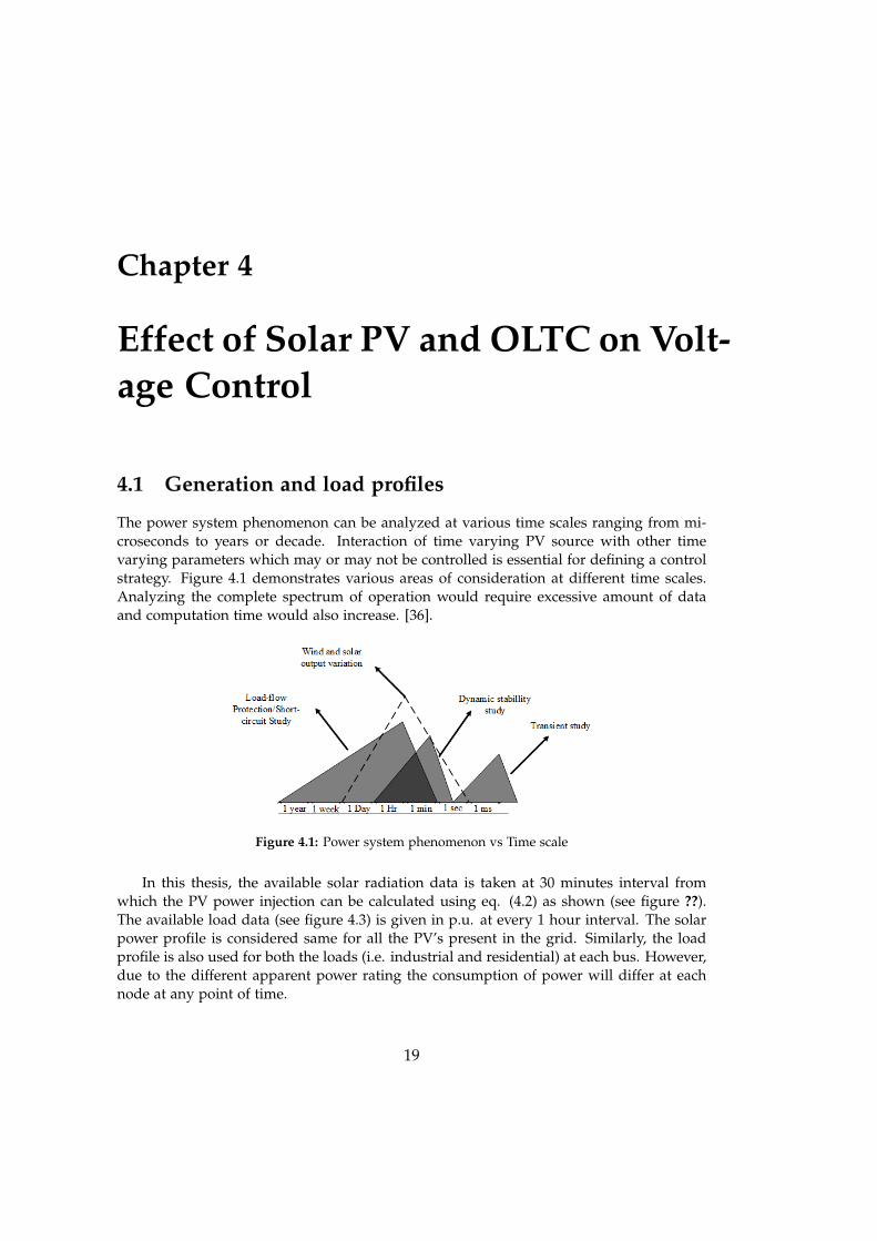
The power system phenomenon can be analyzed at various time scales ranging from mi-croseconds to years or decade. Interaction of time varying PV source with other timevarying parameters which may or may not be controlled is essential for defining a controlstrategy. Figure 4.1 demonstrates various areas of consideration at different time scales.Analyzing the complete spectrum of operation would require excessive amount of dataand computation time would also increase. [36].

Figure 4.1: Power system phenomenon vs Time scale

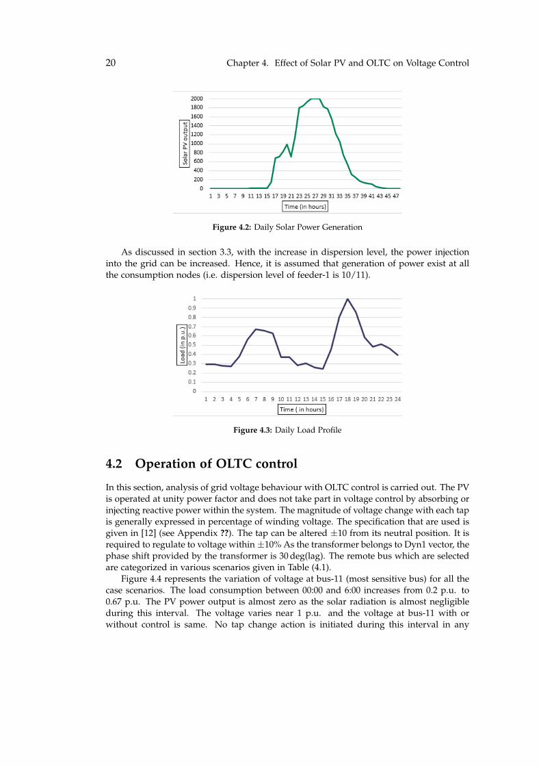
In this thesis, the available solar radiation data is taken at 30 minutes interval fromwhich the PV power injection can be calculated using eq. (4.2) as shown (see figure ??).The available load data (see figure 4.3) is given in p.u. at every 1 hour interval. The solarpower profile is considered same for all the PV’s present in the grid. Similarly, the loadprofile is also used for both the loads (i.e. industrial and residential) at each bus. However,due to the different apparent power rating the consumption of power will differ at eachnode at any point of time.

19

20 Chapter 4. Effect of Solar PV and OLTC on Voltage Control

Figure 4.2: Daily Solar Power Generation

As discussed in section 3.3, with the increase in dispersion level, the power injectioninto the grid can be increased. Hence, it is assumed that generation of power exist at allthe consumption nodes (i.e. dispersion level of feeder-1 is 10/11).

Figure 4.3: Daily Load Profile

4.2 Operation of OLTC control

In this section, analysis of grid voltage behaviour with OLTC control is carried out. The PVis operated at unity power factor and does not take part in voltage control by absorbing orinjecting reactive power within the system. The magnitude of voltage change with each tapis generally expressed in percentage of winding voltage. The specification that are used isgiven in [12] (see Appendix ??). The tap can be altered ±10 from its neutral position. It isrequired to regulate to voltage within ±10% As the transformer belongs to Dyn1 vector, thephase shift provided by the transformer is 30 deg(lag). The remote bus which are selectedare categorized in various scenarios given in Table (4.1).

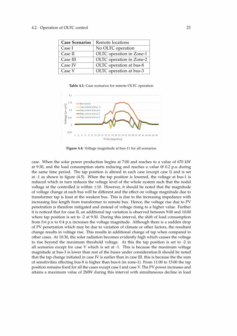
Figure 4.4 represents the variation of voltage at bus-11 (most sensitive bus) for all thecase scenarios. The load consumption between 00:00 and 6:00 increases from 0.2 p.u. to0.67 p.u. The PV power output is almost zero as the solar radiation is almost negligibleduring this interval. The voltage varies near 1 p.u. and the voltage at bus-11 with orwithout control is same. No tap change action is initiated during this interval in any

4.2. Operation of OLTC control 21

Case Scenarios Remote locationsCase I No OLTC operationCase II OLTC operation in Zone-1Case III OLTC operation in Zone-2Case IV OLTC operation at bus-8Case V OLTC operation at bus-3

Table 4.1: Case scenarios for remote OLTC operation

Figure 4.4: Voltage magnitude at bus-11 for all scenarios

case. When the solar power production begins at 7:00 and reaches to a value of 670 kWat 9:30, and the load consumption starts reducing and reaches a value 0f 0.2 p.u duringthe same time period. The tap position is altered in each case (except case I) and is setat -1 as shown in figure (4.5). When the tap position is lowered, the voltage at bus-1 isreduced which in turn reduces the voltage level of the whole system such that the nodalvoltage at the controlled is within ±10. However, it should be noted that the magnitudeof voltage change at each bus will be different and the effect on voltage magnitude due totransformer tap is least at the weakest bus. This is due to the increasing impedance withincreasing line length from transformer to remote bus. Hence, the voltage rise due to PVpenetration is therefore mitigated and instead of voltage rising to a higher value. Furtherit is noticed that for case II, an additional tap variation is observed between 9:00 and 10:00where tap position is set to -2 at 9:30. During this interval, the shift of load consumptionfrom 0.6 p.u to 0.4 p.u increases the voltage magnitude. Although there is a sudden dropof PV penetration which may be due to variation of climate or other factors, the resultantchange results in voltage rise. This results in additional change of tap when compared toother cases. At 10:30, the solar radiation becomes evidently high which causes the voltageto rise beyond the maximum threshold voltage. At this the tap position is set to -2 inall scenarios except for case V which is set at -1. This is because the maximum voltagemagnitude at bus-3 is lower than rest of the buses under consideration.It should be notedthat the tap change initiated in case IV is earlier than in case III. this is because the the sumof sensitivities effecting bus-8 is higher than bus-6 (in zone-1). From 11:00 to 15:00 the tapposition remains fixed for all the cases except case I and case V. The PV power increases andattains a maximum value of 2MW during this interval with simultaneous decline in load


consumption which reaches a value of 0.2 p.u. The PV power production starts declining

Figure 4.5: Variation of tap position

at 15:00 along with increment in load consumption. At this point the voltage magnitudeat bus-6 starts declining and the tap position is shifted to -1 position for Case-4. However,for Case-3 and Case-2 the voltage magnitude is still out of limit and tap position remainsat 2. At 15:30, the further decrease in PV power decreases the voltage magnitude at bus-8also which allows the tap position to return at -1.This action continues with decreasingPV until the voltage magnitude at bus-8 reaches within limit (at 16:00) and when the PVgeneration, becomes reduces at night, all the tap positions are adjusted back to its neutralposition. It should be noted that Case-5 operation shows only single tap position changewhich lasts from 8:00 to 17:30. The OLTC operation time is highest for bus-11 and theleast for Case 3 and 4 both. Also, the OLTC performance for any other bus belongingto that particular zone will have a similar tap response. However, the voltage magnitudemay differ a bit which is insignificant to cause any other kind of variation. As discussed

Figure 4.6: Voltage magnitude at bus-1 for all scenarios

above, the remote control operation of OLTC will regulate its low voltage terminal voltageto compensate the voltage. Figure ??resents bus-1 voltage for all the cases. It can be seenthat the voltage magnitude drops below 0.9 p.u. during the interval when PV is producingpower at its rated capacity. Thus, the voltage regulation achieved through remote controlOLTC operation is insufficient for the duration 10:00 to 16:30. The undervoltage condition

4.3. Q-V Droop Control of PV inverter 23

at bus-1 results in undesirable operation. This suggests that remote control operation ofOLTC in each case requires other measures to control the voltage magnitude of the systemwithin ±10%.

4.3 Q-V Droop Control of PV inverter

In the section, emphasis is given on utilization of PV inverter reactive power capabilitywithout OLTC control. First, the apparent power rating of the inverter of the PV is to bedetermined. In our case, it is assumed to be equal to rated power produced by PV i.e ratingof inverter is 2MVA. The maximum reactive power injection ability is taken to be 44% ofthe MVA name plate rating( i.e. Qrated = 0.968MVAR). In other words, the power factorat which the PV can operate should lie within 0.9 (leading and lagging) when operatingat its rated kVA as suggested in the grid codes [30]. However, the power factor rating ischosen to be unity as the consumer would like to extract all the power produced from thePV panel. Thus, it is required to utilize the available capacity without effecting the realpower generation. Therefore, in this thesis Q-V droop control technique is used. (??).

Figure (4.7). shows a typical Q-V characteristics as given in [37]. When the voltage iswithin the specified limits (V2V3), no reactive power support is provided by the PV. Whenthe voltage is less then minimum voltage of the specified band, the reactive power is in-jected into the system based on the operating voltage and droop setting (vice versa forover-voltage). The droop setting is usually provided by the DSO, therefore it’s impact onthe performance of the grid must be investigated. The specifications provided in [37] isused for calculating droop setting (V3=1.02 and V4=1.08).

Figure 4.7: Q-V droop characteristic for PV system [37]

The rated reactive power delivered by any PV in the system is fixed (Qmax). The droopsettings in case of overvoltage can be calculated as [28]:

m =Q1 −Q2

V1 −V2(4.1)


Voltage-Reactive Default Settings Allowable Setting Rangepower parameters Min MaxVre f VN 0.95VN 1.05VN

V1andV4 Vre f ± 0.08 Vre f − 0.18VNV1 = Vre fV4 = Vre f + 0.18VN

Q1andQ4 44% of MVA rating 0 100 % of MVA rating

V2andV3 Vre f ± 0.02 0V2 = Vre f − 0.03VN

V3 = Vre fQ2andQ3 44% of MVA rating 0 100% of kVA rating

As the voltage magnitude limit is 1.02 for overvoltage condition, the voltage control willbe initiated prior to OLTC control which is operated at ±10% . Therefore, the operation ofvoltage control will be initiated prior to tap control operation with rise in voltage magni-tude beyond the given range.Figure ?? represents variation of voltage magnitude in zone-1 (at bus-11), zone-2 (at bus-6),bus-3 and bus-8. At 7:30, when the solar PV generation is increasing with the sunrise, thevoltage magnitudes in Zone-1 reaches to a value above 1.02 the PV in Zone-1 as well asPV at bus-8 starts absorbing reactive power to bring the voltage at its set point (except forPV at bus-1). As the generation increases and load decreases simultaneously the voltagekeeps rising and the reactive power absorption is increased. Although, the voltage profileshape is almost same, the magnitude differs when the reactive power absorption starts.The reactive power absorption to for each PV is shown in fig 4.8(except PV at Bus-1).

Figure 4.8: Voltage magnitude at bus-11 with and without Q-V control

4.4. Chapter summary 25

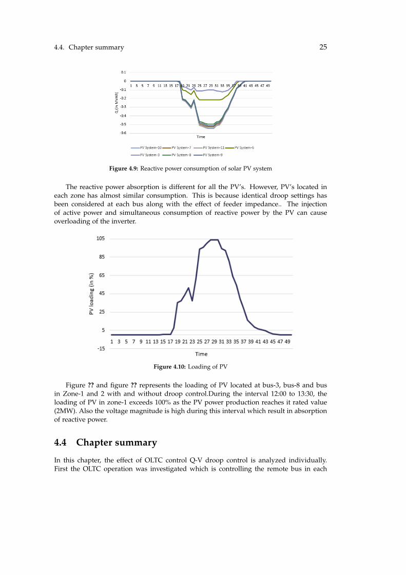
Figure 4.9: Reactive power consumption of solar PV system

The reactive power absorption is different for all the PV’s. However, PV’s located ineach zone has almost similar consumption. This is because identical droop settings hasbeen considered at each bus along with the effect of feeder impedance.. The injectionof active power and simultaneous consumption of reactive power by the PV can causeoverloading of the inverter.

Figure 4.10: Loading of PV

Figure ?? and figure ?? represents the loading of PV located at bus-3, bus-8 and busin Zone-1 and 2 with and without droop control.During the interval 12:00 to 13:30, theloading of PV in zone-1 exceeds 100% as the PV power production reaches it rated value(2MW). Also the voltage magnitude is high during this interval which result in absorptionof reactive power.

4.4 Chapter summary

In this chapter, the effect of OLTC control Q-V droop control is analyzed individually.First the OLTC operation was investigated which is controlling the remote bus in each


zone along with bus-3 and bus-8. It was observed that the number of tap actions is higherin the zone-1 and the least when OLTC is operated at bus-3. Also, the tap position ischanged to -1 in case of bus-3 compared to -2 in case of zone-1. The effect on tap changewas similar for zone-2 and bus-8. However, the duration of tap change is reduced by anhour. The voltage was although regulated at the remote in each case, undervoltage at bus-1 was observed which was beyond ±10% range. In the next section, Q-V droop controlwas used in which nominal settings were used for all PV (except at bus-1). The voltagecontrol performed by the Q-V control restricts all the bus voltage magnitude within thelimits including bus-1. However, the voltage magnitude in zone-1 and 2 was higher ascompared to OLTC tap change. The reactive power consumption was maximum at theweakest bus and least at bus-3. However, for small duration overloading of the PV systemwas observed when the active power generation is at its peak.

Chapter 5

Voltage control using OLTC and DroopControl

5.1 Uncoordinated control of OLTC and Q-V control

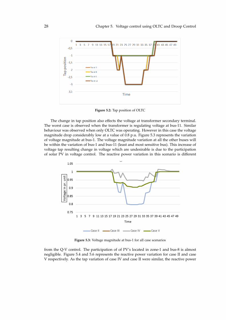
In this section, the effect of OLTC remote control for different cases in presence of Q-Vcontrol performed by the solar PV is analysed. The simultaneous control of voltage byPV and OLTC operating at different voltage control set points (voltage ref. is same i.e. 1p.u.) have an adverse effect on the system. The simulations are analyzed based on thescenarios as given in table 4.1. Figure 5.1 represents the variation of voltage magnitudeat bus-11. It can be inferred that the voltage during each operation is quite low in all thecases as compared to voltage control by OLTC and Q-V control individually (see Fig 4.44.8). The OLTC tap position is significantly effected to due presence of PV voltage control.The range of tap change is increased from -2 to -3 as shown in figure 5.2. The variation oftap change for case-II and case-IV become quite similar. However, the tap change initiatedin case of case-IV is delayed by 30 minutes after which the voltage at bus-8 is regulated.However in case of control performed only OLTC, the variation was similar to as case-IIIcharacteristics. Case-V remains unaffected and the maximum tap position attained is -1.

Figure 5.1: Voltage magnitude at Bus-11 for each case

27

28 Chapter 5. Voltage control using OLTC and Droop Control

Figure 5.2: Tap position of OLTC

The change in tap position also effects the voltage at transformer secondary terminal.The worst case is observed when the transformer is regulating voltage at bus-11. Similarbehaviour was observed when only OLTC was operating. However in this case the voltagemagnitude drop considerably low at a value of 0.8 p.u. Figure 5.3 represents the variationof voltage magnitude at bus-1. The voltage magnitude variation at all the other buses willbe within the variation of bus-1 and bus-11 (least and most sensitive bus). This increase ofvoltage tap resulting change in voltage which are undesirable is due to the participationof solar PV in voltage control. The reactive power variation in this scenario is different

Figure 5.3: Voltage magnitude at bus-1 for all case scenarios

from the Q-V control. The participation of of PV’s located in zone-1 and bus-8 is almostnegligible. Figure 5.4 and 5.6 represents the reactive power variation for case II and caseV respectively. As the tap variation of case IV and case II were similar, the reactive power

5.1. Uncoordinated control of OLTC and Q-V control 29

generated or absorbed by the PV is indistinguishable. Similarly, case II and case IV alsohave similar behaviour. The reactive power is injected to the grid when OLTC is operatingat bus-1. Due to tap change mechanism, the voltage at bus-1 and bus-3 reduces below 0.98.The operating characteristics provided is required to inject reactive power when the volt-age reduces below 0.98 p.u. As the tap change increases the reactive power also increases

Figure 5.4: Reactive power variation of PV for case II

and reaches to a value of 0.5 MVAR. Due to this additional reactive power injection, thetap position reaches a maximum value of -3. However, while simulating case II, the re-active power is being absorbed and reaches a maximum value with change when the tapposition is set to maximum. The injection or absorption of reactive power is higher for PVlocated at bus-3 than any other bus. This is due to the fact that bus-3 is located near thetransformer secondary terminal and as the voltage tap is reduced, the voltage magnitudeat bus-3 also reduces. When the voltage will be minimal at all time in presence of OLTCcontrol. Due to which reactive power is injected to provide voltage support. In case V,

Figure 5.5: Reactive power variation of PV for case-V

the reactive power variation is similar to the scenario when only Q-V droop is operated.However, it should be noted that in case, the magnitude of reactive power absorbed isreduced. Also, PV located in Zone-1 and bus-3 do not take part in voltage control. Since


the real power produced is unaffected, the loading of PV inverter increases beyond 100%during maximum power production. Figure 5.6 represents the loading of PV located atbus-3. Since the power absorbed or injected by any PV in the bus is lower. It is evident

Figure 5.6: Loading of PV at bus-3

from the above discussion that the control of OLTC along with Q-V droop control has tobe coordinated. The number of tap changes along with the maximum tap position.

5.2 Coordinated control of OLTC and PV droop control

This section describes the control strategy adopted for maintaining all the bus voltagein feeder-1 within the ±10% voltage range is discussed. Distributed control techniquesis used which has the features of both centralized control and autonomous control asdiscussed in 2.4. In this case the OLTC is operated as a centralized controller due to whichthe remote control operation is performed simultaneously at all the buses integrated withPV source. As the objective of this thesis is to minimize the tap change ensuring voltagewithin prescribed limits. Figure 5.7 represents the control block diagram according towhich the Q-V control and OLTC control are coordinated for optimum voltage control.The control action is initiated by comparing the actual voltage with dead band providedin the Q-V control (1.02 p.u.). If the voltage is within the limits no control is initiated. Asthe voltage increase beyond the limit, the PV is required to regulated the bus voltage ifthe reactive power capacity is available from the inverter. When there is further increasein the voltage which cannot be regulated by PV, then tap change is initiated. However, thetap position must lie within the specified range. As the OLTC is regulating bus voltagewithin ±10%, the actual voltage is compared with the upper voltage band. If the tapposition is not available or the bus voltage is less than 1.1 p.u., the voltage check for Q-Vcharacteristics is initiated. This closed operation will allow the controllers to maintain thevoltage within permissible value.

5.2. Coordinated control of OLTC and PV droop control 31

Figure 5.7: Control for coordination of OLTC and Q-V droop control

Figure 5.8 represent the variation of voltage magnitude of bus-1 and bus-11. It isevident that the voltage magnitude reaches maximum value of 1.05 at bus-11 while bus-1voltage reaches up to 0.9. It should be noted that in this case the voltage at all the busesare within ±10% range where the voltage magnitudes lie between bus-1 and bus-11.

Figure 5.8: Voltage magnitude at bus-1 and bus-11

The PV inverter at any bus absorbs reactive power as soon as voltage reaches beyond1.02 p.u. The Q-V control will bring back the voltage back to its voltage set point pointvalue depending upon the availability of reactive power capability. When the voltage riseis significant, the Q-V control alone is not sufficient to bring the voltage within limits. Dueto this tap change is initiated by the transformer as shown in figure5.9. It should be notedthat voltage is brought in limits by changing tap position at -1. During this interval, PV


power production reaches to maximum value. When the real power injection is reducedthe tap position is positioned back to neutral position.

Figure 5.9: Tap position of OLTC

Figure 5.10 represents the variation of reactive power of all the PV enabled with Q-Vcontrol. It should be noted that all the PV are contributing in voltage control by absorbingreactive power. However, the reactive power absorbed at each node by the PV is different.This is because the sensitivity of all the buses are different. Due to this rise of voltagemagnitude in zone-2, bus-3 and bus-8 is comparatively lower than the voltage at bus-11.The reactive power absorption begin as the PV power rises.

Figure 5.10: Reactive power output for PV with Q-V control

When the voltage magnitude further increases the tap action is initiated. As the voltageis reduced due to the tap action, reactive power absorbed by the PV reduces (injected

5.3. Chapter Summary 33

back into the grid). This results in less loading of PV inverter (around 101%) which iscomparatively lower compared to uncoordinated control. The loading of transformer is

Figure 5.11: Loading of PV at bus-11

maximum for PV at bus-11 as the reactive power absorbed is higher than any other PVwithin the network. Figure 5.11 represents the loading of PV.

5.3 Chapter Summary

In this chapter evaluation of coordinated control of active distribution network in com-parison to uncoordinated control of OLTC and PV droop control (Q-V). From the resultsobtained, it is clear that number of tap change is reduced from 1 to 3. Also, the maximumtap deviation is reduced as the PV operates at maximum position of -1. The reactive powerabsorbed or generated by the PV depends on the PV location and the remote bus selectedfor regulating the voltage. The loading of the PV is also reduced to a certain extent. How-ever, it is impossible to reduce the loading below 100% during peak interval as the realpower produced by the PV is equal to MVA rating of the PV.

Chapter 6

Conclusions and Future Work

6.1 Conclusions

In this thesis fundamental principles are worked out which are generally used in voltagecontrol. With the rising solar PV system in the grid, effective management using coor-dinated control is developed. At first the MV grid is analyzed using sensitivity analysis.Based on the sensitivity relation of each bus different zones were established. Bus-3 andbus-8 were considered individually as their sensitivities were different from buses in anyzone. The consumers should be allowed to integrate PV system with the grid to increasecompetitiveness in the market. Hence, an investigation was carried out varying dispersionand penetration level. It was observed that with increase of dispersion level the maximumallowed power injection can be increased significantly. However, when the same power isproduced with less dispersion level, the voltage magnitude increases.In the next chapter OLTC control is used for regulating the bus voltage in the active dis-tribution network. Remote control in the defined zones as well as at bu-3 and bus-8 wereinvestigated. It was observed that when bus-3 is regulated the number of tap changed re-quired is less. Regulating the weakest bus results in undervoltage at bus-1. Selecting anybus within the zone will result in similar behavior in voltage magnitude variation. In thenext section Q-V droop control technique was used. The voltage bandwidth in which PVoperates is lower than OLTC. Due to this Q-V droop will regulate voltage at much lowerlevel. It was observed that all the voltages were within the limits however the the magni-tude was higher as compared to OLTC operation. The loading of PV also increases withincrease in reactive power absorption. When the OLTC and Q-V droop are operated simul-taneously without any coordination, the tap change requirement increases. With propercoordinated control as proposed, the tap change is minimized and the voltage magnitudeare also under permissible range.

6.2 Future Work

This section enlists several relevant ideas which can be implemented in future work. Inthis thesis, quasi-dynamic analysis has been analyzed. Hence an investigation of dynamicbehaviour can be implemented. Furthermore, detailed model of PV can be implemented

35

36 Chapter 6. Conclusions and Future Work

rather than a static generator. Impact of other type of autonomous control and its per-formance evaluation in presence of OLTC can also be investigated. Additional regulatingunits such as shunt capacitors, energy storage devicss can aslo be included

Bibliography

[1] Global Market Outlook 2019-2023 - SolarPower Europe. http://www.solarpowereurope.org/global-market-outlook-2019-2023/. (Accessed on 07/22/2019).

[2] METIS Study-Effect of high shares of renewables on power systems. https://www.irena.org/-/media/Files/IRENA/Agency/Publication/2018/Feb/IRENA_REmap_EU_2018.pdf. (Accessed on 07/22/2019).

[3] Model Analysis of Flexibility of the Danish Power System. https://ens.dk/sites/ens.dk/files/Globalcooperation/Publications_reports_papers/model_analysis_of_flexibility_of_the_danish_power_system.2018.05.15.pdf. (Accessed on 07/22/2019).

[4] Effect of high shares of renewables on power systems - Publications Office of the EU.https://publications.europa.eu/en/publication-detail/-/publication/01c456f4 - 7144 - 11e9 - 9f05 - 01aa75ed71a1 / language - en / format - PDF /source-96288175. (Accessed on 07/22/2019).

[5] M Karimi, H Mokhlis, K Naidu, et al. “Photovoltaic penetration issues andimpacts in distribution network–A review”. In: Renewable and Sustainable En-ergy Reviews 53 (2016), pp. 594–605.

[6] Ferry A Viawan, Ambra Sannino, and Jaap Daalder. “Voltage control withon-load tap changers in medium voltage feeders in presence of distributedgeneration”. In: Electric power systems research 77.10 (2007), pp. 1314–1322.

[7] Bianca Barth Zuzana Musilova Paolo Michele Sonvilla Carlos Mateo Ric-cardo Lama et al. European Advisory Paper. https://ec.europa.eu/energy/intelligent/projects/sites/iee-projects/files/projects/documents/pv_grid_european_advisory_paper_july_2014_annex_ii.pdf. Apr. 2018.

[8] Xiaohu Liu, Andreas Aichhorn, Liming Liu, et al. “Coordinated control ofdistributed energy storage system with tap changer transformers for voltagerise mitigation under high photovoltaic penetration”. In: IEEE Transactions onSmart Grid 3.2 (2012), pp. 897–906.

37

http://www.solarpowereurope.org/global-market-outlook-2019-2023/

http://www.solarpowereurope.org/global-market-outlook-2019-2023/

https://www.irena.org/-/media/Files/IRENA/Agency/Publication/2018/Feb/IRENA_REmap_EU_2018.pdf



https://ens.dk/sites/ens.dk/files/Globalcooperation/Publications_reports_papers/model_analysis_of_flexibility_of_the_danish_power_system.2018.05.15.pdf




https://publications.europa.eu/en/publication-detail/-/publication/01c456f4-7144-11e9-9f05-01aa75ed71a1/language-en/format-PDF/source-96288175



https://ec.europa.eu/energy/intelligent/projects/sites/iee-projects/files/projects/documents/pv_grid_european_advisory_paper_july_2014_annex_ii.pdf



38 Bibliography

[9] Ellen Liu and Jovan Bebic. Distribution system voltage performance analysis forhigh-penetration photovoltaics. Tech. rep. National Renewable Energy Lab.(NREL),Golden, CO (United States), 2008.

[10] Satoru Akagi, Shinya Yoshizawa, Jun Yoshinaga, et al. “Capacity determina-tion of a battery energy storage system based on the control performanceof load leveling and voltage control”. In: Journal of International Council onElectrical Engineering 6.1 (2016), pp. 94–101.

[11] Kashem M Muttaqi, An DT Le, Michael Negnevitsky, et al. “A coordinatedvoltage control approach for coordination of OLTC, voltage regulator, andDG to regulate voltage in a distribution feeder”. In: IEEE Transactions on In-dustry Applications 51.2 (2015), pp. 1239–1248.

[12] Stefano Barsali et al. Benchmark systems for network integration of renewable anddistributed energy resources. 2014.

[13] K Prakash, A Lallu, FR Islam, et al. “Review of power system distributionnetwork architecture”. In: 2016 3rd Asia-Pacific World Congress on ComputerScience and Engineering (APWC on CSE). IEEE. 2016, pp. 124–130.

[14] DigSilent. PowerFactory User Manual. https://www.digsilent.de/en/. (Ac-cessed on 09/01/2019). 2019.

[15] Rene Prenc, Davor Škrlec, and Vitomir Komen. “A novel load flow algo-rithm for radial distribution networks with dispersed generation”. In: Tech-nical Gazette 20.6 (2013), pp. 969–977.

[16] Dusko Nedic. “Tap adjustment in AC load flow”. In: UMIST. 2002.

[17] CL Wadhwa. Electrical power systems. New Age International, 2006.

[18] Turan Gonen. Electric power distribution engineering. CRC press, 2015.

[19] “IEEE Recommended Practice for Electric Power Distribution for IndustrialPlants”. In: IEEE Std 141-1993 (1994), pp. 1–768. doi: 10.1109/IEEESTD.1994.121642.

[20] Ferry Viawan. Voltage control and voltage stability of power distribution systemsin the presence of distributed generation. Chalmers University of Technology,2008.

[21] Dr. Dieter Dohnal. On-Load Tap-Changers For Power Transformers. https://www.reinhausen.com/de/XparoDownload.ashx?raid=58092. (Accessed on08/08/2019).

[22] J-H Choi and J-C Kim. “The online voltage control of ULTC transformer fordistribution voltage regulation”. In: International Journal of Electrical Power &Energy Systems 23.2 (2001), pp. 91–98.

[23] Math HJ Bollen and Fainan Hassan. Integration of distributed generation in thepower system. Vol. 80. John wiley & sons, 2011.

https://www.digsilent.de/en/

https://doi.org/10.1109/IEEESTD.1994.121642

https://doi.org/10.1109/IEEESTD.1994.121642

https://www.reinhausen.com/de/XparoDownload.ashx?raid=58092

https://www.reinhausen.com/de/XparoDownload.ashx?raid=58092

Bibliography 39

[24] Bo Zhao, Xuesong Zhang, and Jian Chen. “Integrated microgrid laboratorysystem”. In: IEEE Transactions on power systems 27.4 (2012), pp. 2175–2185.

[25] Joan Rocabert, Alvaro Luna, Frede Blaabjerg, et al. “Control of power con-verters in AC microgrids”. In: IEEE transactions on power electronics 27.11(2012), pp. 4734–4749.

[26] A Tuladhar, H Jin, T Unger, et al. “Parallel operation of single phase in-verter modules with no control interconnections”. In: Proceedings of APEC97-Applied Power Electronics Conference. Vol. 1. IEEE. 1997, pp. 94–100.

[27] Hua Han, Xiaochao Hou, Jian Yang, et al. “Review of power sharing controlstrategies for islanding operation of AC microgrids”. In: IEEE Transactions onSmart Grid 7.1 (2015), pp. 200–215.

[28] N Karthikeyan, Basanta Raj Pokhrel, Jayakrishnan R Pillai, et al. “Coordi-nated voltage control of distributed PV inverters for voltage regulation inlow voltage distribution networks”. In: 2017 IEEE PES Innovative Smart GridTechnologies Conference Europe (ISGT-Europe). IEEE. 2017, pp. 1–6.

[29] Askari Mohammad Bagher, Mirzaei Mahmoud Abadi Vahid, and MirhabibiMohsen. “Types of solar cells and application”. In: American Journal of opticsand Photonics 3.5 (2015), pp. 94–113.

[30] D Energinet. “Technical regulation 3.2. 2 for PV power plants with a poweroutput above 11 kW”. In: Tech. Rep. (2015).

[31] Erhan Demirok, Pablo Casado Gonzalez, Kenn HB Frederiksen, et al. “Localreactive power control methods for overvoltage prevention of distributed so-lar inverters in low-voltage grids”. In: IEEE Journal of Photovoltaics 1.2 (2011),pp. 174–182.

[32] John J Grainger, William D Stevenson, William D Stevenson, et al. Powersystem analysis. 2003.

[33] HM Ayres, W Freitas, MC De Almeida, et al. “Method for determiningthe maximum allowable penetration level of distributed generation withoutsteady-state voltage violations”. In: IET generation, transmission & distribution4.4 (2010).

[34] Fracisco M González-Longatt et al. “Impact of distributed generation overpower losses on distribution system”. In: 9th International conference on electri-cal power quality and utilization. 2007.

[35] Deependra Singh, Devender Singh, and KS Verma. “Multiobjective optimiza-tion for DG planning with load models”. In: IEEE transactions on power sys-tems 24.1 (2009), pp. 427–436.

40 Bibliography

[36] Alexandra Von Meier. “Integration of renewable generation in California:Coordination challenges in time and space”. In: 11th International Conferenceon Electrical Power Quality and Utilisation. IEEE. 2011, pp. 1–6.

[37] Dispersed Generation Photovoltaics and Energy Storage. “IEEE Standard forInterconnection and Interoperability of Distributed Energy Resources withAssociated Electric Power Systems Interfaces”. In: ().

coordinated voltage control in active distribution network with … · coordinated voltage control...

Documents