convergent cutting-plane and partial-sampling …castlelab.princeton.edu/html/papers/chen...

JOURNAL OF OPTIMIZATION THEORY AND APPLICATIONS: Vol. 102, No. 3, pp. 497-524, SEPTEMBER 1999

Convergent Cutting-Plane and Partial-SamplingAlgorithm for Multistage Stochastic Linear

Programs with Recourse1

Z. L. CHEN2 AND W. B. POWELL3

Communicated by M. Avriel

Abstract. We propose an algorithm for multistage stochastic linearprograms with recourse where random quantities in different stages areindependent. The algorithm approximates successively expected recoursefunctions by building up valid cutting planes to support these functionsfrom below. In each iteration, for the expected recourse function in eachstage, one cutting plane is generated using the dual extreme points ofthe next-stage problem that have been found so far. We prove that thealgorithm is convergent with probability one.

Key Words. Multistage stochastic programming, cutting planes, sam-pling, convergence with probability one.

1. Introduction

Numerous real-world problems in applications, such as transportation(Ref. 1), production planning (Ref. 2), financial planning (Ref. 3), and manyother fields (Refs. 4 and 5), can be formulated as two-stage or multistagestochastic linear programs with recourse. The characteristics of such a prob-lem can be summarized as follows: (i) a stage usually represents a timeperiod; (ii) the very beginning of the first stage is viewed as here and now;(iii) at the beginning of each stage, we know deterministically all the datain this stage, but know only probabilistically all the data in future stages;

1This work was supported in part by Grant AFOSR-F49620-93-1-0098 from the Air ForceOffice of Scientific Research.

2Assistant Professor, Department of Systems Engineering, University of Pennsylvania, Phila-delphia, Pennsylvania.

3Professor, Department of Civil Engineering and Operations Research, Princeton University,Princeton, New Jersey.

4970022-3239/99/0900-0497$16.00/0 © 1999 Plenum Publishing Corporation

498 JOTA: VOL. 102, NO. 3, SEPTEMBER 1999

(iv) at the beginning of the first stage, decisions must be made before therealization of random data in future stages; (v) once random data in a stagebecomes known, correction (i.e., recourse) actions are allowed to compens-ate the decisions for this stage made earlier; (vi) the goodness of the decisionmaking is measured by the total cost, consisting of the deterministic cost inthe first stage and total expected cost in the future stages.

Methods for stochastic linear programs can be generally classified intothose which use a fixed sample of realizations (scenario-based methods)and those which iteratively sample realizations as the algorithm progresses(sampling-based methods).

Scenario-based methods normally approximate a stochastic problemusing a relatively small set of realizations which allow the problem to besolved as a (typically large) linear program. Two-stage problems may beapproximated using hundreds or in special cases thousands of scenarios, butmultistage problems are normally restricted to much smaller samples. Oncea set of scenarios has been generated, most scenario-based methods treatthis sample as representing the entire problem which they then strive to solveto optimality. Examples of algorithms designed for this class of problemsincludes the diagonal quadratic approximation method of Mulvey and Rusz-czynski (Ref. 6), augmented Lagrangian decomposition method of Rosaand Ruszczynski (Ref. 7), L-shaped method of Van Slyke and Wets (Ref.8), its generalization to multistage problems by Birge (Ref. 9), and scenarioaggregation method of Rockafellar and Wets (Ref. 10). All these algorithmsprovide optimal solutions to what are normally approximations of the origi-nal problem.

Sampling-based methods represent explicitly the complete sample space,which may be of infinite size for all practical purposes. Examples includethe stochastic linearization method (Refs. 11 and 12), auxiliary functionmethod (Ref. 13), stochastic decomposition (Ref. 14), sample path optimiza-tion (Ref. 15), and stochastic hybrid approximation method (Ref. 16). Allthese methods use successive samples to develop algorithms that convergein some probabilistic sense in the limit. In practical settings, statisticalmethods have to be used to determine convergence criteria and the solutionproperties after a finite number of iterations (Ref. 14).

A popular strategy to counteract the exponential growth of multistagemodels has been to develop successive approximations of the recourse func-tion. It is well known (see, for example, Refs. 8 and 17) that the expectedrecourse function in a two-stage program can be replaced with a series ofBenders cuts, where the recourse function is represented using a fixed sample.Birge (Ref. 9) extends this approach to multistage problems by proposinga nested Benders decomposition algorithm. The basic version of this methodinvolves a forward pass through the time periods, using a specific set of cuts,

JOTA: VOL. 102, NO. 3, SEPTEMBER 1999 499

and then a backward pass, where new cuts are generated. Other authorshave studied variations of this strategy (Refs. 18-22). Infanger and Morton(Ref. 23) show how the method can be extended to take advantage ofinterstage dependencies.

Nested Benders decomposition, as it is generally described (see forexample Ref. 23), requires solving a linear program at each time period andfor each scenario, where a scenario represents a full history of events up tothat point in time. Let i, represent the set of outcomes in time period /,and let ht = (w1, w 2 , . . . , w t ) represent the history of the process, whereh,eHt = O1 x O2 x • • • x Ot (some authors use the notation Ot to representthe history, whereas we use it only to denote events within a time period).Clearly, the size of Ht grows exponentially with the number of stages, makingnested Benders decomposition impractical for even medium-sized problems.

In this paper, we propose a new convergent algorithm for multistagestochastic linear programs with recourse that satisfy the followingassumptions:

(Al) random quantities in different stages are independent;(A2) the sample space of random quantities in each stage is discrete

and finite;(A3) random quantities appear only on the right-hand side of the

linear constraints in each stage;(A4) the feasible region of the problem in each stage is always non-

empty and bounded.

As mentioned earlier, Assumption (A2) is necessary for all scenario-based methods. Assumptions (A3) and (A4) are made in many sampling-based methods including the stochastic decomposition method of Higle andSen (Ref. 14). The nested Benders decomposition method of Birge (Ref. 9)assumes (A2) and (A3). We note that the result that we are going to presentcan be extended, after some refinement, to more general cases including thecase where not only the right-hand side vectors, but also the matrices Bt

linking neighboring stages are stochastic, and also including the case wherethe feasible region of the problem in each stage can be infeasible orunbounded.

Features of our method include:

(a) At each iteration, we solve a linear program for a single realizationwteQt (as opposed to each h,eH t) at each stage t. As a result,the computational requirements of the procedure per iterationgrow linearly with the number of stages and the size of the samplespace per stage.

(b) We perform a simple comparison over the entire sample space Qt

at each stage t. Thus, Qt may be large (say, in the tens or evenhundreds of thousands), but must be finite.

(c) Our method successively approximates the expected recourse func-tion by building up valid cutting planes to support these functionsfrom below.

(d) We prove that the algorithm converges in the limit, but do notprovide finite convergence.

Because we use only a partial sample [item (a) above], rather than thefull sample required by other methods, we call our method cutting-planeand partial-sampling (CUPPS) algorithm. On the other hand, the full passover the sample space in item (b) implies that the space must be finite, incontrast with true sampling techniques such as stochastic decomposition.Our method is closest to the nested Benders decomposition method of Birge(Ref. 9) and stochastic decomposition method of Higle and Sen (Ref. 14).

The research contribution of the paper is the presentation of a newalgorithm for solving multistage stochastic programs, which is convergentin probability, and which is computationally tractable for problems withlarge numbers of outcomes per stage and large numbers of stages. Theprimary limitation of our method is shared by all cutting-plane algorithms,which is slow convergence when we are approximating high-dimensionalityproblems. Since the relative advantage of CUPPS over the classical nestedBenders decomposition in terms of execution time per iteration is obvious,we do not present any numerical experiments. Our belief is that experimentalwork must be conducted in the context of a specific application with analgorithm that is able to take advantage of the structure of that problem.

This paper is organized as follows. In Section 2, we present the coreidea of the CUPPS algorithm when applied to a two-stage problem andcompare it to the L-shaped algorithm and stochastic decomposition algo-rithm. In Section 3, we present the details of the CUPPS algorithm.In Section 4 we give some preliminary results, and in Section 5 we establishthe convergence of this algorithm. Finally, we conclude the paper in Section6.

2. Core Idea and Comparison

In this section, we present briefly the core idea of our CUPPS methodwhen applied to a two-stage problem and compare it to the two closestexisting methods: the stochastic decomposition (SD) method of Higle andSen (Ref. 14) and L-shaped (LS) method of Van Slyke and Wets (Ref. 8).



We begin by introducing some basic notation:

(Qt, Ft, Pt) = probability space of the random quantities in stage t, whereQt is the sample space of the random quantities [hence by (A2), |Qt| isfinite]; Ft is a a-algebra and P, a probability measure defined over Qt;Qt= {wt ,.. ., wt,qi } = sample space of the random quantities in stage t,where qt = \Qt\ and (wti is a sample in Qt, Vi= 1 , . . . , qt, with q1 = 1;pti=probability associated with each sample wt,eQt, W = l , . . . ,q t , suchthat Eq1t=1 pti=1;Ht= a-field which represents the information available up to stage t;x, = vector of decisions in stage t;ct= vector of cost in stage t;A, = constraint matrix in stage t;Bt = constraint matrix linking stage t and stage t + 1;Q r ( x t - 1 , w t ) = Qt(xr-1,wt |Ht-1) = recourse function in stage t — 1 given thehistory Ht-1; note that Assumption (Al) guarantees the first equality;Q t (x t - 1 ) = Zq t i = lp t iQt(x t-1 ,Wt l)=En iQT(x,- l ,wl) = E o l Q t ( X l - l , w t \ H l - l ) =expected recourse function in stage t— 1 given the history Ht-1; note thatAssumption (Al) guarantees the second equality.

A general T-stage stochastic linear program with recourse can be formu-lated as follows:

For the problem of our interest that satisfies Assumption (Al), the formula-tion (1) can be rewritten equivalently in the following recursive form:


where the recourse function is defined by, for t = 2,

and QT+1=0.The core idea of the CUPPS method is to successively approximate the

expected recourse function in each stage by valid cutting planes that aregenerated based on a known subset of dual extreme points of the next-stageproblem. To be specific, let us consider the two-stage problem given by (2-7) with T=2. For solving this problem, each iteration k of the CUPPSalgorithm involves two steps.

The first step solves an approximated problem LP1, which is as follows:

where (10) represents the k cuts generated so far. These cuts are generatedin the second step and approximate the expected recourse function Q2(x1)by supporting it from below. Note that initially the algorithm approximatesQ2(xi) by the first cut that is trivial, z> -oo. Let xk1 denote the solution toproblem (8-11).

In the second step, first the algorithm randomly draws a sample,denoted as wk2 from Q2, then solves problem LP2 with x1=xk1 and0)2 = 0)2. Assumption (A4) guarantees that both the optimal primal anddual solutions to this problem can always be found. Let nk be the dualsolution of this problem. Notice that, in problem LP2, x1 and w2 appearonly on the right-hand side. Thus, for any given xu1 and xv1 with u=v, andfor given w2t, w2jeQ2 with i=j, any dual extreme point of problem LP2

with x1 = xu1 and w2 =w2i is also a dual extreme point of the problem withxt=xu 1 and w2 = w2j. Let

be the set of all dual extreme points of problem LP2 generated up to iterationk. Based on the dual extreme points in Dk, the algorithm then generates anew cut,


with coefficients (scalar ak+1 and vector Bk+1) given by

Note that, for large problems, the summation over all possible outcomes inQ2 in Eq. (13) and the maximum operator applied in Eq. (14) represent thecomputational bottleneck of the procedure.

As we show in Section_4, the cut generated this way is valid for theexpected recourse function Q 2 (x 1 ) , in that it supports Q2(w1) from below,but may not be tight, as illustrated in Fig. 1, top. The effort for generating

Fig. 1. Comparison of cuts generated by the CUPPS, SD, and LS methods.


this cut involves solving one linear program (that is, problem LP2 withXi =xk

1,w2 =w2k) and O(kq2) basic operations for computing ak+1 and Bk+1

in (13) and (14). This cut is then added to problem (8-11). The wholeprocedure is then repeated.

By comparison, the SD algorithm shares similar steps, except that itnot only generates new cuts, but also updates previously generated cuts. Bycontrast, the LS algorithm, not only solves just one problem LP2 withx1=xk

1 and w2 =w2k, but instead it solves every problem LP2 with x1=xk

1

and w2= w 2 j , V j = 1 , . . . , q2. Then, a new cut is generated based on theoptimal dual solutions of all these q2 problems.

Specifically, in the SD algorithm, iteration k solves problem LP2 withx1 = xk

1 and 0)2 = 0)2 and generates a new cut (12) with coefficients ak+1 andBk+1 given by

In general, the cut generated this way may not be a valid cut for the expectedrecourse function Q2(x1), as illustrated in Fig. 1 (center) because thecoefficients of the cut are computed in (15) using only k samples, instead ofall the samples in Q2. It is easy to see that the computational effort involvedhere is solving one linear program and performing O(k) basic operations in(15) and (16); indeed, in iteration k, one computes only rrk, since all otherrrj, with 1<j<k-1, were computed earlier. Thus, the SD algorithm offersthe lowest computational effort per iteration of all three algorithms.

To generate a new cut in iteration k, the LS algorithm solves everyproblem LP2 with x1 =xk

1 and w2 = w 2 j , for each j=1 , . . . , q2. Let ukj denote

the optimal dual solution (obtained in iteration k) of problem LP2 withx1=xk

1 and w2 =w2j. Then, the coefficients of the new cut (12) generatedby the LS algorithm in iteration k are given by

It is easy to see that ak+1 and Bk+1 given by (17) satisfy

Furthermore, it is not difficult to see that the cut given by (17) is valid;hence, by (18), it is a tight cut for the expected recourse function Q2(x1)


and touches the function at the point xk1, as shown in Fig. 1 (bottom). The

computational effort involved here consists of solving q2 linear programsand performing O(q2) basic operations in (17).

From the above comparison, it is quite clear that, to generate a cut,the LS algorithm needs the most computational effort, while the SD algo-rithm needs the least computational effort among these three algorithms.On the other hand, the quality of the cuts generated by the LS algorithm isthe best in terms of their tightness. Thus, for two-stage problems, the CUPPSalgorithm can be viewed as a method lying between the SD algorithm andthe LS algorithm. The CUPPS algorithm attempts to build valid cuts, insteadof stochastic cuts as in the SD algorithm, by using available dual extremepoints that have been generated, instead of solving all the problems associ-ated with the samples as in the LS algorithm.

For multistage problems, the core ideas of the nested Benders decompo-sition algorithm of Birge (Ref. 9) and of the CUPPS algorithm are similarto their respective counterparts for two-stage problems described above.Hence, we do not compare them here. The details of the CUPPS algorithmare described in Section 3. See Ref. 9 for the details of the nested Bendersdecomposition algorithm.

3. CUPPS Algorithm

In each iteration, the CUPPS algorithm solves an approximated prob-lem LPt, denoted as APt for each t= 1 , 2 , . . . , T— 1, and a problem LPT.In problem APt, the expected recourse function Q t + 1 (x t ) is approximatedby some cuts that support it from below. After solving problem APt or LPT,the algorithm generates a cut that is valid for the expected recourse functionQt (xt -1) and adds this cut to problem AP t -1. In the course of the algorithm,the approximated problems APt, for t=1, . . . ,T-1, approximate theoriginal LP, more and more accurately.

In each iteration, the algorithm generates one cut for each expectedrecourse function Q t(x t-1) for t = 2,..., T. At the very beginning, the algo-rithm uses the following initial cut to support the function Q t ( x t - i ) frombelow:

Certainly, this is a valid cut. Thus, there are a total of k +1 cuts in problemAPt right after iteration k.


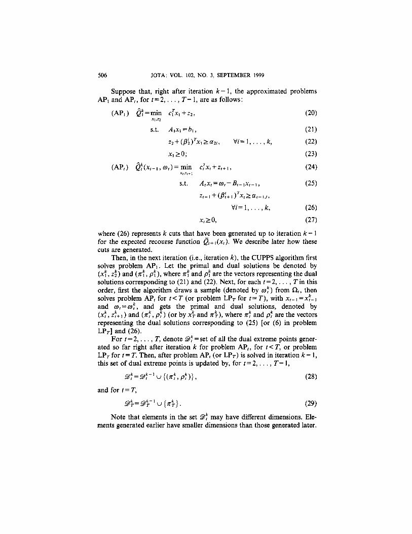
Suppose that, right after iteration k-1, the approximated problemsAP1 and APt, for t = 2,..., T- 1, are as follows:

where (26) represents k cuts that have been generated up to iteration k -1for the expected recourse function Q t + 1 (x t ) . We describe later how thesecuts are generated.

Then, in the next iteration (i.e., iteration k), the CUPPS algorithm firstsolves problem AP1. Let the primal and dual solutions be denoted by(xk1, zk2) and (nk1,pk1), where rk1 and pk1 are the vectors representing the dualsolutions corresponding to (21) and (22). Next, for each t = 2, . .. , Tin thisorder, first the algorithm draws a sample (denoted by (wkt) from Qt, thensolves problem AP, for t<T (or problem LPT for t=T), with xt-1 = xkt-1

and wt = wkt, and gets the primal and dual solutions, denoted by(xkt,zkt+1) and (xkt, Zkt+1) (or by xkT and nkr), where nkt and pkt are the vectorsrepresenting the dual solutions corresponding to (25) [or (6) in problemLPT] and (26).

For t=2 , . . . , T, denote Dkt = set of all the dual extreme points gener-ated so far right after iteration k for problem APt, for t<T, or problemLPT for t=T. Then, after problem APt (or LPT) is solved in iteration k — 1 ,this set of dual extreme points is updated by, for t = 2 T — 1 ,

and for i=T

Note that elements in the set Dkt may have different dimensions. Ele-ments generated earlier have smaller dimensions than those generated later.


Throughout this paper, whenever we calculate the inner product of or com-pare two vectors with different dimensions, we assume that the vector withsmaller dimension is extended by attaching zeros to it such that it has thesame dimension as the other vector. We show in Section 5 that any elementin Dkt generated earlier than iteration k, if extended accordingly by attachingzeros to it, is still a dual extreme point of problem APt formed later thaniteration k.

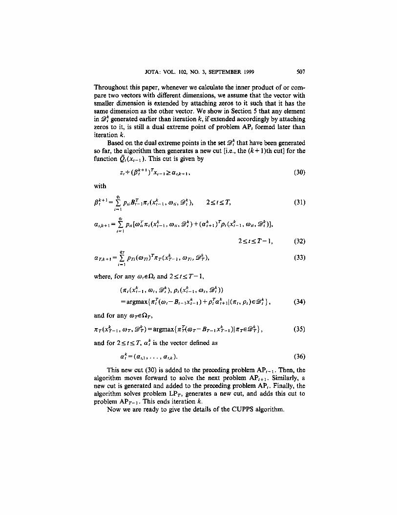
Based on the dual extreme points in the set Dkt that have been generatedso far, the algorithm then generates a new cut [i.e., the (k+ l)th cut] for thefunction Q t ( x t - 1 ) . This cut is given by

with

where, for any O,eO, and 2<t<T-1,

and for any

and for 2<1<T,a|is the vector defined as

This new cut (30) is added to the preceding problem APt-1. Then, thealgorithm moves forward to solve the next problem APt+1. Similarly, anew cut is generated and added to the preceding problem AP,. Finally, thealgorithm solves problem LPT, generates a new cut, and adds this cut toproblem APT-1. This ends iteration k.

Now we are ready to give the details of the CUPPS algorithm.


CUPPS Algorithm.

Step O. For t= 1, 2 , . . . , T — 1 , formulate the initial approximatedproblem APt with only one initial cut given by (19). Let theset of dual extreme points D1t = o for all t = 2, 3 , . . . , T. Setthe iteration counter k = 1.

Step 1. Solve problem AP1. Get the optimal primal solution (xk1,zk2)and optimal solution value Qk1.

Step 2. For t = 2, . . ., T- 1 in this order, do the following. Draw arandom sample (wkt from Qt. For given xt-1 = xkt-1 andwt=wkt, solve problem APt. Get the optimal primal solution(xkt, zkt+1), optimal solution value Qkt(xk t -1,wkt), and optimaldual solution (rk t , pkt). Get the latest set of dual extremepoints Dkt by (28). Generate the (k+ l)th cut given by (30).Add this cut to problem APt-1.

Step 3. Draw a random sample (wkT from QT. For xT - 1= xkT-1 andwT=wk T, solve problem LPt. Get the optimal primal solutionxkT, optimal solution value Q T ( X k t - 1 , wkt), and optimal dualsolution nkT. Get the latest set of dual extreme points DkT by(29). Generate the (k+ l)th cut given by (30) with t= T. Addthis cut to problem APT-1.

Step 4. Set k = k+l; go to Step 1.

4. Preliminary Results

In this section, we prove that all the cuts generated in the CUPPSalgorithm for the expected recourse function Q,(x,-1), Vt = 2,..., T, arevalid; that is, they support Q , ( x , - 1 ) from below. Also, we give two basicresults that are used in Section 5.

Define, for any k>1 and 1< t<T-1,

Lemma 4.1. In the CUPPS algorithm, each cut added to problemAPT-1 is a valid cut for the function Q T ( X T - 1 ).

Proof. Clearly, in problem A P t - 1 , the very first cut given by (19) witht = T- 1 is valid for Q T (x T - 1 ) . Now, consider the kth cut in APT-1 for anyk>2. Clearly, for any given XT-1 and wTi, for any i=1, . . . ,qT , nT

( X k T - 1 , w T i , D k T ) is a dual feasible solution to problem LPT with a given


First multiplying by pTt, then summing over all i on the both sides, we have

This shows that the kth cut in APT-1 is valid for Q T ( X t - 1 ) . D

Lemma 4.2. In the CUPPS algorithm, for any t with 1 < t<T-1, andfor any k with K> 1, every element in the set Dk

t is a dual extreme point ofproblem APt formed right after any iteration j with j>k-1.

Proof. First, it is easy to see that any element (n t , pt) in the set Dkt

is a dual extreme point of problem APt generated in some iteration i withi<k. Let DP1 denote the dual of problem APt formed right after iterationi-1. Then, (n t , pt ) is an extreme point of problem DP1. Let DP2 denotethe dual of problem APt formed right after iteration j for any given j>k.Then, in order to prove the lemma, we only need to show that (n t , pt ),

if

extended by adding a proper number of zeros to its end, is also an extremepoint of problem DP2.

Since the algorithm adds one cut to problem APt in each iteration, andonce a cut is added it will always be there, problems DP1 and DP2 are thesame, except that in DP2 there are j-i more columns. Thus, (n t , pt ) isfeasible to DP2 if we extend it by adding j—i zeros to its end. Denote thisextended vector by (n t , p

+t), where

In the following, we show that (nt, pt+ ) is an extreme point of DP2.

We prove it by contradiction. If it is not, then there exist two differentsolutions of DP2, denoted by (n1

t, p1t ) and (r2

t, p2t ), such that

XT-1 and wt=wTi. This implies that, for any XT-1 and i= 1,. . ., qT,


Clearly,

Hence, by (37), we have that

Now, define two vectors p1t and p2

t with dimension i such that

Then, the fact that (r1t, p1

t)=(n2t, p2

t) implies that

and (38) implies that

On the other hand, it is easy to show that both (n1t, p

it) and (n2,, p2,) are

feasible for DPI. Then, (39) and (40) are in contradiction with the fact that(nt, p,) is an extreme point of DPI. This shows that (nt, pt

+ ) must be anextreme point of DP2. D

Lemma 4.3. In the CUPPS algorithm, for any r = 1,_..., T- 1, eachcut added to problem APr is a valid cut for the function Q r + 1 ( x t ) .

Proof. We prove this by induction on T. For r = T-1, this result hasbeen proved in Lemma 4.1. Now, assume that, for any given t< T- 1, thisresult is true for r = t. We need to prove that this result is also true for t =t — 1 . For any given k> 1, it is easy to see that, right after iteration k, problemAPt is equivalent to the following problem:

where Fkt + 1(x t) is a piecewise linear function formed by the k cuts in (26).

By the induction assumption, these cuts are valid for the functionQt+1(xt); then,

On the other hand, the feasible region of problem (41) is the same as thatof problem LPt. So, it must be true that the optimal objective function valueof problem (41) is no more than that of problem LPt; i.e., for any xt-1 andwt,


Taking expectation of both sides, we have

On the other hand, by Lemma 4.2, any element in Dkt is a dual extreme

point of problem APt in iteration k. Thus, for any w t ieQ t,with 1 <i<qt,the vector (rt(xk

t-1,wt, Dkt), p t ( x k

t - 1 , w t i , D kt ) ) is a dual extreme point of

problem APt in iteration k. This means that, for any xt-1 and i = 1 , . . . , q,,

First multiplying by pti, then summing over all i on the both sides, we have

Together with (42), this gives

This shows that the (k+ l)th cut in problem AP t -1 , generated right afterproblem APt is solved in iteration k, is a valid cut for the function Q t ( x t - 1 ) .This shows that the result is true when r = t — 1 . Therefore, by induction,we have shown the lemma. D

Lemma 4.4. The following properties all hold:

Proof. These results are straightforward from Lemmas 4.1 and 4.3.Thus, we omit the proofs for them. D


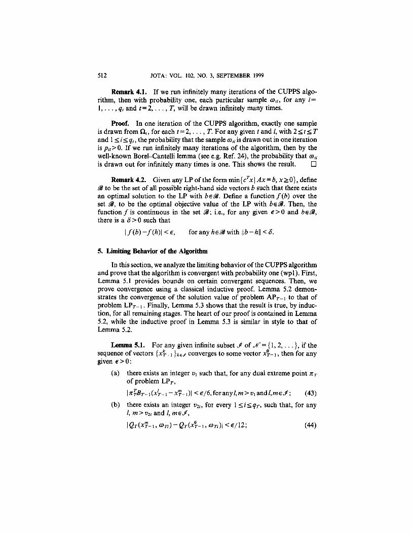
Remark 4.1. If we run infinitely many iterations of the CUPPS algo-rithm, then with probability one, each particular sample wti, for any i=1 , . . . ,qt and t = 2 , . . . , T, will be drawn infinitely many times.

Proof. In one iteration of the CUPPS algorithm, exactly one sampleis drawn from Qt, for each t = 2,...,T. For any given t and i, with 2<,t<Tand 1<i<q t , the probability that the sample wti is drawn out in one iterationis pti>0. If we run infinitely many iterations of the algorithm, then by thewell-known Borel-Cantelli lemma (see e.g. Ref. 24), the probability that wti,is drawn out for infinitely many times is one. This shows the result. D

Remark 4.2. Given any LP of the form min{cTx \ Ax = b, x > 0}, defineB to be the set of all possible right-hand side vectors b such that there existsan optimal solution to the LP with bEB. Define a function f(b) over theset B, to be the optimal objective value of the LP with be38. Then, thefunction f is continuous in the set B; i.e., for any given e>B and beSS,there is a 5 > 0 such that

5. Limiting Behavior of the Algorithm

In this section, we analyze the limiting behavior of the CUPPS algorithmand prove that the algorithm is convergent with probability one (wpl). First,Lemma 5.1 provides bounds on certain convergent sequences. Then, weprove convergence using a classical inductive proof. Lemma 5.2 demon-strates the convergence of the solution value of problem APT-1 to that ofproblem LPT-1. Finally, Lemma 5.3 shows that the result is true, by induc-tion, for all remaining stages. The heart of our proof is contained in Lemma5.2, while the inductive proof in Lemma 5.3 is similar in style to that ofLemma 5.2.

Lemma 5.1. For any given infinite subset i of N = {1, 2, . . .}, if thesequence of vectors {Xk

t-1 }kei converges to some vector X OT - 1 , then for any

given e>0:

(a) there exists an integer v1 such that, for any dual extreme point rT

of problem LPT,

(b) there exists an integer v2i, for every 1 <,i<qT, such that, for any/, m>v2i and l, mei,


furthermore, let v2 = max {v 2 1 , v 2 2 , . . . , v2qr}; for any I,m>v2 and/, meJ, and 1 <,i<,qT, we have

(c) there exists an integer u3 such that, for any m>u3 and meJ,

Proof.

(a) Assume that we are given a dual extreme point nT of problemLPr. By Assumption (A4), we can assume \nT\ < Yfor some finite positivenumber Y. The convergence of the sequence [Xk

T-1 }kej implies that thesequence {BT-1 x

kT-1 }kej is also convergent. Thus, for any given e > 0, there

exists some integer v1 such that, for any l ,m>v1 and I, mej, we have

which implies that, V/, m> v1 and l,meJ,

This shows (a).(b) By Remark 4.2, for any given wr, the function Q T ( x T - 1 , w T ) is

continuous in X T - 1 . For any i with 1<i<,qT, consider the functionQ T ( X T - 1 , w T i ) at point X ° T - 1 . By the continuity of this function, for anye>0, there exists Si>0 such that, if \ \XT - 1-X0

T - 1 l \<8 i , then

On the other hand, since {XkT-1 }kej is convergent, then for a given £i, there

exists an integer v2l such that, for any m>v2l and m e j , we have

All this implies (44), which further implies that, V/, m>v2i and l,meS,

Let u2 = max{v21,v22,• • •, v2 p T}. Then, we have the result (45). This shows(b).

(c) Similarly, the function QT-1 (xT-2, wo

T-I ) is continuous in x T - 2 .We can use a similar argument to prove (46). D


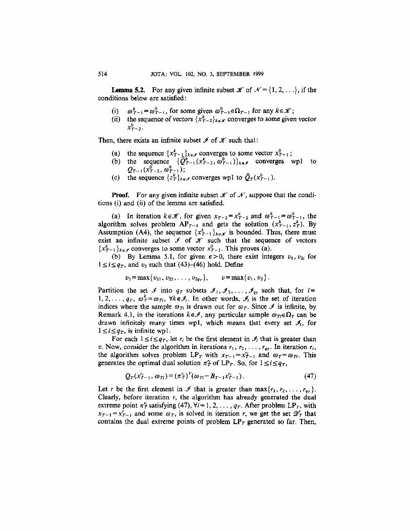
Lemma 5.2. For any given infinite subset K of N = {1,2,...}, if theconditions below are satisfied:

(i) (wkt-1 = w°T-1, for some given w 'r-1efiT-1 for any k e k ;

(ii) the sequence of vectors {XKT-2}kek converges to some given vector

v°XT-2-

Then, there exists an infinite subset I of k such that:

(a) the sequence {x kT - 1 }kej converges to some vector X0

T-1;(b) the sequence { Q k

T - 1 ( x kT - 2 , w 0

T - 1 ) } k e J converges wpl toQT-1(x°T-2,w

0T-1);

(c) the sequence { z kT } k e j converges wpl to Q T ( X ° T - I ) .

Proof. For any given infinite subset k of N, suppose that the condi-tions (i) and (ii) of the lemma are satisfied.

(a) In iteration kej , for given xT-2 = xkT-2 and wk

T-1 = w0T-1, the

algorithm solves problem APT-1 and gets the solution ( x kT - 1 , z k

T ) . ByAssumption (A4), the sequence {xk

T-\}keX is bounded. Thus, there mustexist an infinite subset ./ of k such that the sequence of vectors{Xk

T-1 }kej converges to some vector x°T-1. This proves (a).(b) By Lemma 5.1, for given e>0, there exist integers v 1 ,v 2 1 for

1 <i<qT, and v3 such that (43)-(46) hold. Define

Partition the set j into qT subsets J1 ,J2 , . . . ,J9T such that, for i =1, 2 , . . ., qT, wk

T=wTi, VkeJ i. In other words, ji is the set of iterationindices where the sample wTi is drawn out for wT. Since J is infinite, byRemark 4.1, in the iterations keJ, any particular sample wTieQT can bedrawn infinitely many times wpl, which means that every set jt, for1 <i<qT, is infinite wpl.

For each 1<,i<qT, let ri be the first element in A that is greater thanv. Now, consider the algorithm in iterations r1, r2,. .., rqr. In iteration rt,the algorithm solves problem LPT with X T - 1 = x r T - 1 and w=wTi. Thisgenerates the optimal dual solution rr

T of LPT. So, for 1 <*i<>qT,

Let r be the first element in j that is greater than max{r1, r2,. . . , r q T } .Clearly, before iteration r, the algorithm has already generated the dualextreme point rr

T satisfying (47), Vi= l , 2 , . . . , q T . After problem LPT, withXT-1 =xr

T-1 and some wT, is solved in iteration r, we get the set DrT that

contains the dual extreme points of problem LPT generated so far. Then,


the (r + l)th cut for the function Q T (x T - 1 ) is generated and added to prob-lem APT - 1 . This cut is given by

where the vector BTr+1 and the scalar aT,r+1 are defined in (31) with t=T

and k = r and in (33) with k = r; that is,

where

It is easy to see that

Thus, (51) implies that, for each i= 1 ,2 , . . . , qT,

Now, let

Let N be the first element in J that is greater than s. Consider any iterationn, with n>N and n e j . In iteration n, the algorithm solves problem APT-1 ,with xT-2

=XnT-2 and wT-1

= w0T-1, and gets the solution value

QnT-1(x

nT-2, w0

T-1) and the solution (xnT - 1 ,zn

T) . Note that, since n>r, initeration n the cut (48) is already in problem APT_1. Hence, the solution(xn

T-1, ZnT) must satisfy (48), that is,


For notational convenience, we define

By (47) and (52), Inequality (53) implies

Inequality (54) implies

It is easy to see that xT - 1=x nT - 1 is a feasible solution to problem LPT-1 ,

with XT-2=xnT-2 and wT-1 = w°T-1, which means that

Combining (55) and (56), we get

On the other hand, by Lemma 4.4,

From (57) and (58), it is not difficult to show that


This gives

It is easy to see that

Hence, by (43) and (45), we have

Similarly, since n > u3, by (46) we have

Thus, (60) and (61) imply

This means that the sequence {QkT-1(x

kT-2, wo

T-1)}kej converges toQT-I (x

oT-2, w

oT-1 )• Since in the proof we have used the result that each Jt

is infinite wpl, this convergence is wpl. This shows part (b) of the lemma,(c) The convergence of the sequence {zk

T}ksj can be proved similarlyas follows. The relations (55) and (58) imply

Then, by (56), we have

This, together with (54), implies


By (44), we have

This, together with (61) and (62), implies

Hence, the sequence {zkT}kes converges wpl to QT(X°T-I). This shows part

(c) of the lemma. D

Now, we demonstrate convergence of all other stages.

Lemma 5.3. For any given r, 1 < T < T- 2, and any given infinite sub-set k of N = {1, 2 , . . .} , if the conditions below are satisfied:

(i) wkT = w°r for some given wo

TeQr, for any k e k ;(ii) the sequence of vectors {xk

T-1}kek converges to some given vectorxo

T-1.

Then, there exists an infinite subset J of K such that:

(a) the sequence {xkT}keJ converges to some vector xo

T;(b) the sequence {Qk

T(xkr-i, wo

T)}kej converges wpl to

Qr(xoT-1,X

OT);

(c) the sequence {zkT+1}kej converges wpl to QT +1(x°T).

Proof. We prove the lemma by induction on T. When T = T-1, thislemma is exactly Lemma 5.1 and hence holds. Suppose that this lemmaholds when r = t. We need to prove that it also holds when t = t—\. Theproof technique is similar to that of Lemma 5.2. Thus, we provide only asketch of proof.

For any given infinite subset k of N, suppose that, when r = t — 1 ,conditions (i) and (ii) of the lemma are satisfied.


(a) In iteration k e k , the algorithm solves problem APT-1, withxt-2

= xkt- 2 and wt -1 = wo

t-1, and gets the solution (x kt - 1 ,z

kt) . By Assumption

(A4), the sequence {x kt - 1} k e k is bounded. Thus, there must exist an infinite

subset l of k such that the sequence of vectors {x kt - 1 } k e j converges to

some vector xot-1.

Partition the set l into q, subsets l1, l2 yqt such that, for i =1,2,. . . ,q t ,

wkt = wti, V k e j i .

In other words, ji is the set of iteration indices where the sample wti isdrawn out for wt. By Remark 4.1, it is easy to see that every set Li, for1 <:i<qt, is infinite wpl.

For each i= 1, 2 , . . . , qt, by the induction assumption that the lemmaholds for r = t and by the facts that wk

t = wti, for all keL i , and that thesequence {x k

t - 1} k e l [hence, the sequence { x k , - } } k e l i ] converges to somevector x°t-1, there must exist a subset li of jt, for each i=1,2 , . . . ,q , , suchthat the sequence { Q k

t ( x kt - 1 , w t i ) } k e j i converges wpl to Q t(x° t -1,w t i ). Thus,

it is easy to show that, for any given e>0, there exists an integer ui suchthat, wpl,

Define

Clearly, J<&. Hence, the sequence {x kt - 1} k e j converges to xo

t-1. Thisshows that part (a) of the lemma holds when r = t-1.

(b) First, using (63) and logic similar to that in the proof of Lemma5.1, we can get the following results for any given e>0:

(i) there exists an integer v1 such that, for any dual extreme point(rt, pt) of problem APt,

(ii) there exists an integer v2i, for every 1 <,i^q,, such that

furthermore, let v2=max{u1, u2, . . . ,uq t , v21, v22,..., u2qt}; wehave


(iii) there exists an integer u3 such that

Let us define v, ri for 1 <i<,qt, r, s, and N exactly in the same way asin the proof of Lemma 5.2. Consider the algorithm in iterations ri and r.Similar to (47) and (52), the following relations hold for each i=1,2 qt:

Now, consider any iteration n and n>N and nej. In iteration n, thealgorithm solves problem AP t - 1 , with given xt-2 = xn

t-2 and wt-i = wot-1,

and gets the solution value Qnt-i(x

nt-2, wo

t - 1-i) and the solution (tf-\, 2?,)Since n>r, in iteration n the (r+ l)th cut, with coefficients Br

t+1 and at,r+1

defined by (31) and (32), is already in problem APt-1. Hence, the solution(xn

t-1, znt) must satisfy that cut; that is,

By (68) and (69), we can get a result similar to (54) as follows:

where


Using the same argument as in the proof of Lemma 5.2, we can then showthe following result that is similar to (60):

By (64) and (66), we have

Similarly, by (67), we have

Thus, (71) implies

This means that the sequence {Qkt-1(xk

t-2, wot-1)}kej converges to

Qt-1 (xot-2,wo

t-1). Since in the proof we have used some results that are truewpl, this convergence is wpl. This shows that part (b) of the lemma holdswhen r = t-1.

(c) The convergence of the sequence {zkt}ksj can be proved similarly

to part (c) of Lemma 5.2. We do not give any details here.Therefore, by induction, we have proved the lemma. D

Theorem 5.1. The sequence of solution values {Qkt}keN of problem

AP1 converges wpl to the optimal value Q1.

Proof. In the approximated problem AP1, we can view the constraintA1x1=b1 as A1x1 = w1-BoXo , with (w1 = b1, x0 = 0, and any given B0; and1we can view the value Qk

1 as the function Q kt (X 0 , (w1). Thus, when T = 1 and

k = N, the conditions (i) and (ii) of Lemma 5.3 are certainly satisfied.Applying Lemma 5.3, we have that there exists an infinite subset J of N,such that the sequence {Q k

t } k e j converges wp1 to Q1(b1, 0) = Q1.On the other hand, by Lemma 4.4, the sequence {Qk

t }keN is nondecreas-ing. We know that, if a monotone sequence has a convergent subsequencethat converges to some value, then the whole sequence must converge tothat value. Therefore, the sequence {Qk

t}keN converges wpl to Q1. D

Theorem 5.2. Any accumulation point of the sequence {xkt }keN is an

optimal solution wpl of problem LP1.

Proof. To prove this, we need to show only that any convergent subse-quence of the sequence {xk

t}keN converges wpl to an optimal solution ofproblem LP1.


Consider a subsequence k of N such that the sequence [xk1 }k e k con-

verges to some vector x01. With the identification b0 = w1-Box0 as in the

proof of Theorem 5.1, applying Lemma 5.3, we can show that there existsa_subsequence J of k, such that the sequence {z k

2} k s j converges wpl toQ2(x

01).

On the other hand, we know that

Thus,

Now, in the set k, we take the limit on both sides of (73). Since the sequence{xk

1}kek converges to x01, and since by Theorem 5.1 the sequence

{Qk1}kek converges wpl to Q1, then the sequence {zk

2}kek, converges wplto Q1 - cT

1x01. We know that, if a convergent sequence has a subsequence

that converges to some value, then the whole sequence converges to thatvalue, so the following must be true:

Hence,

Since xk1 is a feasible solution to problem LP1, for any k e k , then by

Assumption (A4), the limit x°1 of the sequence {xk1 }kejr must be a feasible

solution to problem LP1. Therefore, (74) implies that the solution x°1 isactually optimal to problem LP1. This shows the theorem. D

6. Conclusions

In this paper, we have proposed the CUPPS algorithm, a sampling-based algorithm, for solving multistage stochastic linear programs. We haveproved that the algorithm is convergent with probability one.

We believe that multistage stochastic linear programs are much harderthan two-stage ones. It is unlikely that a scenario-based algorithm is capableof solving a multistage problem with the sample space in each stage contain-ing 1000 samples. For such a problem with T as small as 3, there are 106

scenarios. Standard methods, such as the diagonal quadratic approximationmethod of Mulvey and Ruszczynski (Ref. 6) and augmented Lagrangiandecomposition method of Rosa and Ruszczynski (Ref. 7), that reformulatethe stochastic problems as a deterministic equivalence, are certainly incap-able of dealing with such a problem. We also doubt that the nested Benders

decomposition algorithm of Birge (Ref. 9) can handle such a problem,because one iteration alone involves solving at least 3000 linear programs.We believe that sampling-based methods that require only to solve a smallnumber of linear programs in each iteration are more likely to be successfulin solving multistage stochastic linear programs involving a large numberof samples in each stage. The CUPPS algorithm proposed in this paper isthe first such method that is convergent for multistage stochastic linearprograms.

References

1. POWELL, W. B., JAILLET, P., and ODONI, A., Stochastic and Dynamic Networksand Routing, Handbook in Operations Research and Management Science, Vol-ume on Networks, Edited by C. Monma, T. Magnanti, and M. Ball, NorthHolland, Amsterdam, Holland, pp. 141-295, 1995.

2. ESCUDERO, L. F., KAMESAM, P. V., KING, A. J., and WETS, R., ProductionPlanning via Scenario Modeling, Annals of Operations Research, Vol. 43,pp. 311-335, 1993.

3. MULVEY, J. M., and VLADIMIROU, H., Stochastic Network Programming forFinancial Planning Problems, Management Science, Vol. 38, pp. 1642-1664,1992.

4. BIRGE, J. R., Stochastic Programming Computation and Applications, INFORMSJournal on Computing, Vol. 9, pp. 111-133, 1997.

5. BIRGE, J. R., and MULVEY, J. M., Stochastic Programming in Industrial Engin-eering, Technical Report, Department of Industrial and Operations Engineering,University of Michigan, 1996.

6. MULVEY, J. M., and RUSZCZYNSKI, A., A Diagonal Quadratic ApproximationMethod for Large-Scale Linear Programs, Operations Research Letters, Vol. 12,pp. 205-215, 1991.

7. ROSA, C., and RUSZCZYNSKI, A., On Augmented Lagrangian DecompositionMethods for Multistage Stochastic Programs, Annals of Operations Research,Vol. 64, pp. 289-309, 1996.

8. VAN SLYKE, R., and WETS, R., L-Shaped Linear Programs with Applicationsto Optimal Control and Stochastic Programming, SIAM Journal on AppliedMathematics, Vol. 17, pp. 638-663, 1969.

9. BIRGE, J. R., Decomposition and Partitioning Techniques for Multistage Stochas-tic Linear Programs, Operations Research, Vol. 33, pp. 989-1007, 1985.

10. ROCKAFELLAR, T. R., and WETS, R., Scenarios and Policy Aggregation in Opti-mization under Uncertainty, Mathematics of Operations Research, Vol. 16,pp. 119-147, 1991.

11. GUPAL, A. M., and BAZHENOV, L. G., A Stochastic Method of Linearization,Cybernetics, Vol. 8, pp. 482-484, 1972.

12. ERMOLIEV, Y., Stochastic Quasigradient Methods and Their Application to Sys-tem Optimization, Stochastics, Vol. 9, pp. 1-36, 1983.



13. CULIOLI, J. C., and COHEN, G., Decomposition /Coordination Algorithms inStochastic Optimization, SIAM Journal on Control and Optimization, Vol. 28,pp. 1372-1403, 1990.

14. HIGLE, J. L., and SEN, S., Stochastic Decomposition: An Algorithm for Two-Stage Linear Programs with Recourse, Mathematics of Operations Research,Vol. 16, pp. 650-669, 1991.

15. ROBINSON, S. M., Analysis of Sample Path Optimization, Mathematics of Opera-tions Research, Vol. 21, pp. 1-528, 1996.

16. CHEUNG, R. K. M., and POWELL, W. B., A Stochastic Hybrid ApproximationProcedure, with an Application to Dynamic Networks, Technical Report SOR-94-02, Department of Civil Engineering and Operations Research, PrincetonUniversity, 1994.

17. WETS, R., Programming under Uncertainty: The Solution Set, SIAM Journal onApplied Mathematics, Vol. 14, pp. 1143-1151, 1966.

18. WITTROCK, R. J., Advances in a Nested Decomposition Algorithm for SolvingStaircase Linear Programs, Technical Report SOL-83-2, Stanford University,1983.

19. GASSMAN, H. I., MSLIP: A Computer Code for the Multistage Stochastic LinearProgramming Problem, Mathematical Programming, Vol. 47, pp. 407-423, 1990.

20. PEREIRA, M. V. F., and PINTO, L. M. V. G., Multistage Stochastic OptimizationApplied to Energy Planning, Mathematical Programming, Vol. 52, pp. 359-375,1991.

21. INFANGER, G., Planning under Uncertainty: Solving Large-Scale Stochastic Lin-ear Programs, Boyd and Fraser, Scientific Press Series, New York, New York,1994.

22. MORTON, D. P., An Enhanced Decomposition Algorithm for Multistage StochasticHydroelectric Scheduling, Annals of Operations Research, Vol. 64, pp. 211-235,1996.

23. INFANGER, G., and MORTON, D. P., Cut Sharing for Multistage StochasticLinear Programs with Interstate Dependency, Mathematical Programming, Vol.75, pp. 241-256, 1996.

24. CHUNG, K. L., A Course in Probability Theory, Academic Press, New York,New York, 1974.

convergent cutting-plane and partial-sampling …castlelab.princeton.edu/html/papers/chen...

Documents