Control Systems

Lect.8 Root Locus TechniquesBasil Hamed

Chapter Learning Outcomes

After completing this chapter the student will be able to:• Define a root locus (Sections 8.1-8.2)• State the properties of a root locus (Section 8.3)• Sketch a root locus (Section 8.4)• Find the coordinates of points on the root locus and

their associated gains (Sections 8.5-8.6)• Use the root locus to design a parameter value to

meet a transient response specification for systems of order 2 and higher (Sections 8.7-8.8)

Basil Hamed 2

Root Locus – What is it?• W. R. Evans developed in 1948.• Pole location characterizes the feedback system

stability and transient properties.• Consider a feedback system that has one parameter

(gain) K > 0 to be designed.

• Root locus graphically shows how poles of CL system varies as K varies from 0 to infinity.

Basil Hamed 3

L(s): open-loop TF

Root Locus – A Simple Example

Basil Hamed 4

Characteristic eq.

K = 0: s = 0,-2K = 1: s = -1, -1K > 1: complex numbers

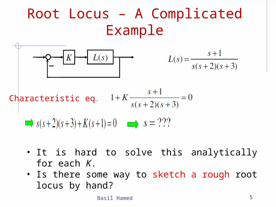
Root Locus – A Complicated Example

Basil Hamed 5

Characteristic eq.

• It is hard to solve this analytically for each K.• Is there some way to sketch a rough root locus by

hand?

8. 1 Introduction• Root locus, a graphical presentation of the closed-loop poles as a

system parameter is varied, is a powerful method of analysis and design for stability and transient response(Evans, 1948; 1950).

• Feedback control systems are difficult to comprehend from a

qualitative point of view, and hence they rely heavily upon mathematics.

• The root locus covered in this chapter is a graphical technique that gives us the qualitative description of a control system's performance that we are looking for and also serves as a powerful quantitative tool that yields more information than the methods already discussed.

Basil Hamed 6

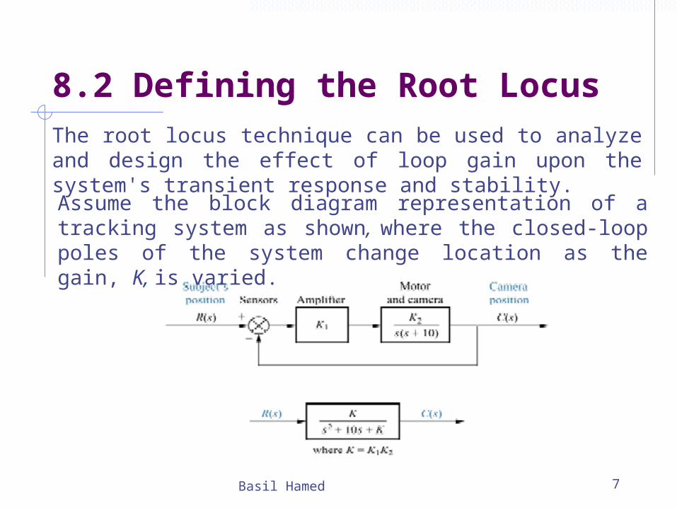
8.2 Defining the Root LocusThe root locus technique can be used to analyze and design the effect of loop gain upon the system's transient response and stability.

Basil Hamed 7

Assume the block diagram representation of a tracking system as shown, where the closed-loop poles of the system change location as the gain, K, is varied.

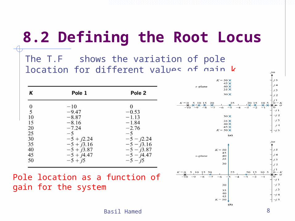
8.2 Defining the Root LocusThe T.F shows the variation of pole location for different values of gain k.

Basil Hamed 8

Pole location as a function of gain for the system

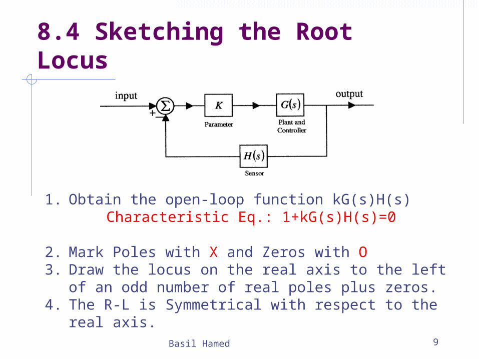
8.4 Sketching the Root Locus

Basil Hamed 9

1. Obtain the open-loop function kG(s)H(s) Characteristic Eq.: 1+kG(s)H(s)=0

2. Mark Poles with X and Zeros with O3. Draw the locus on the real axis to the left of an odd number of real

poles plus zeros.4. The R-L is Symmetrical with respect to the real axis.

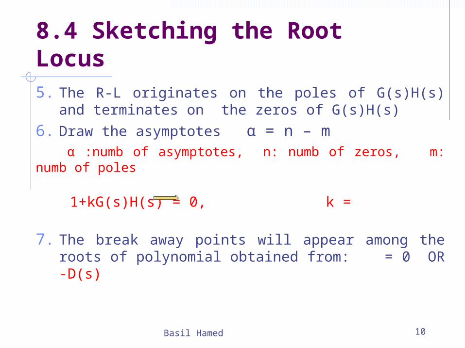
8.4 Sketching the Root Locus5. The R-L originates on the poles of G(s)H(s) and terminates on the

zeros of G(s)H(s)

6. Draw the asymptotes α = n – m α :numb of asymptotes, n: numb of zeros, m: numb of poles

1+kG(s)H(s) = 0, k =

7. The break away points will appear among the roots of polynomial obtained from: = 0 OR -D(s)

Basil Hamed 10

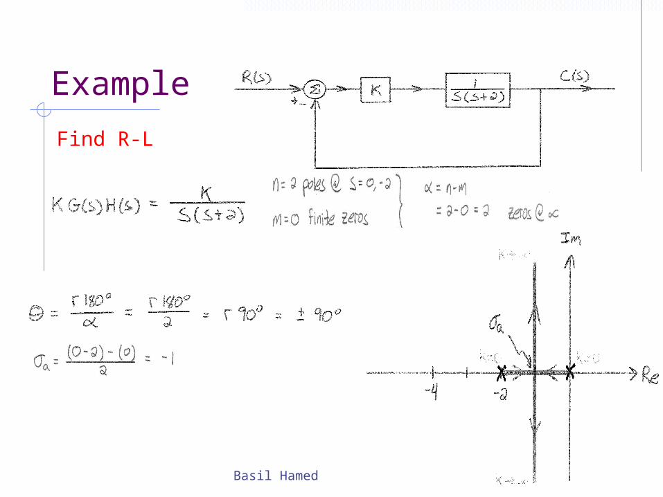
Example

Basil Hamed 11

Find R-L

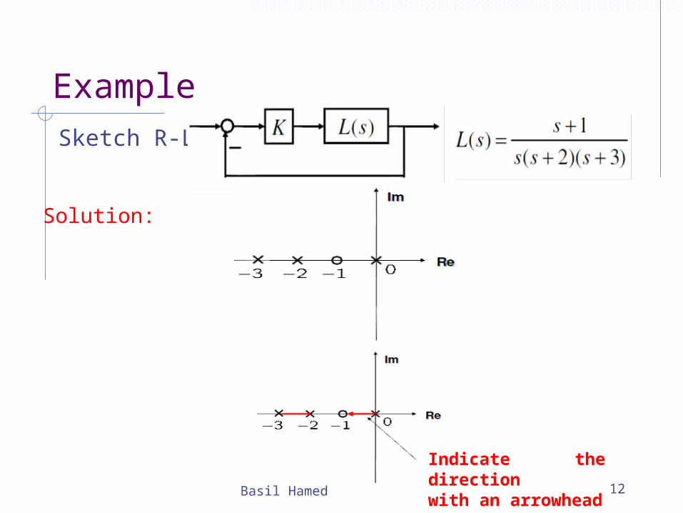
ExampleSketch R-L

Basil Hamed 12

Solution:

Indicate the directionwith an arrowhead

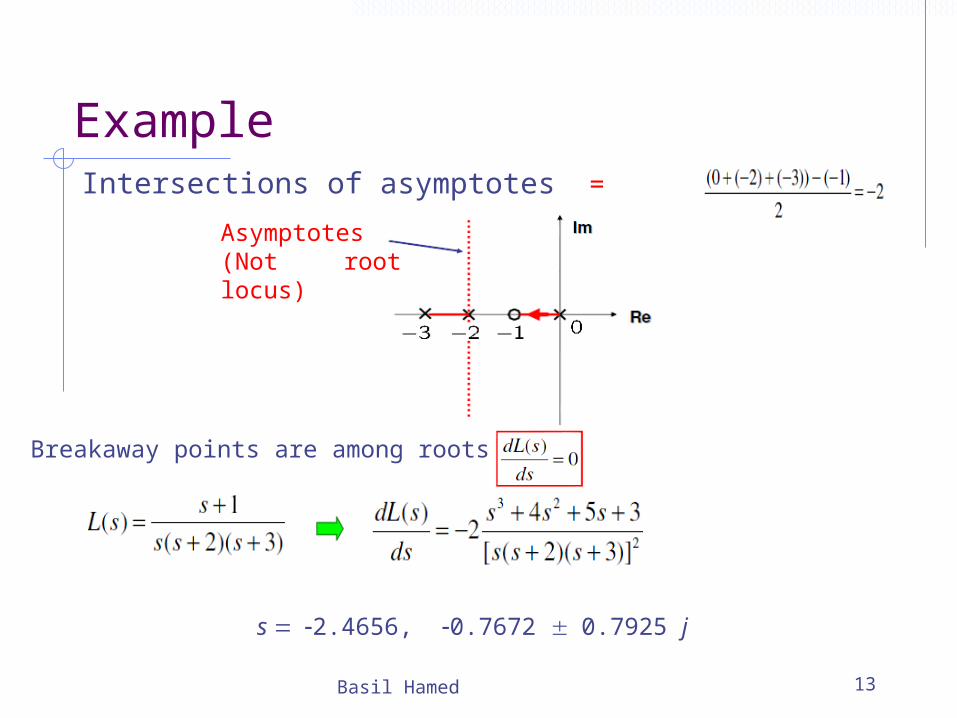
ExampleIntersections of asymptotes =

Basil Hamed 13

Asymptotes(Not root locus)

Breakaway points are among roots of

s = -2.4656, -0.7672 ± 0.7925 j

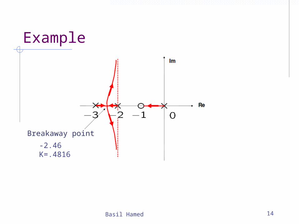
Example

Basil Hamed 14

Breakaway point

-2.46K=.4816

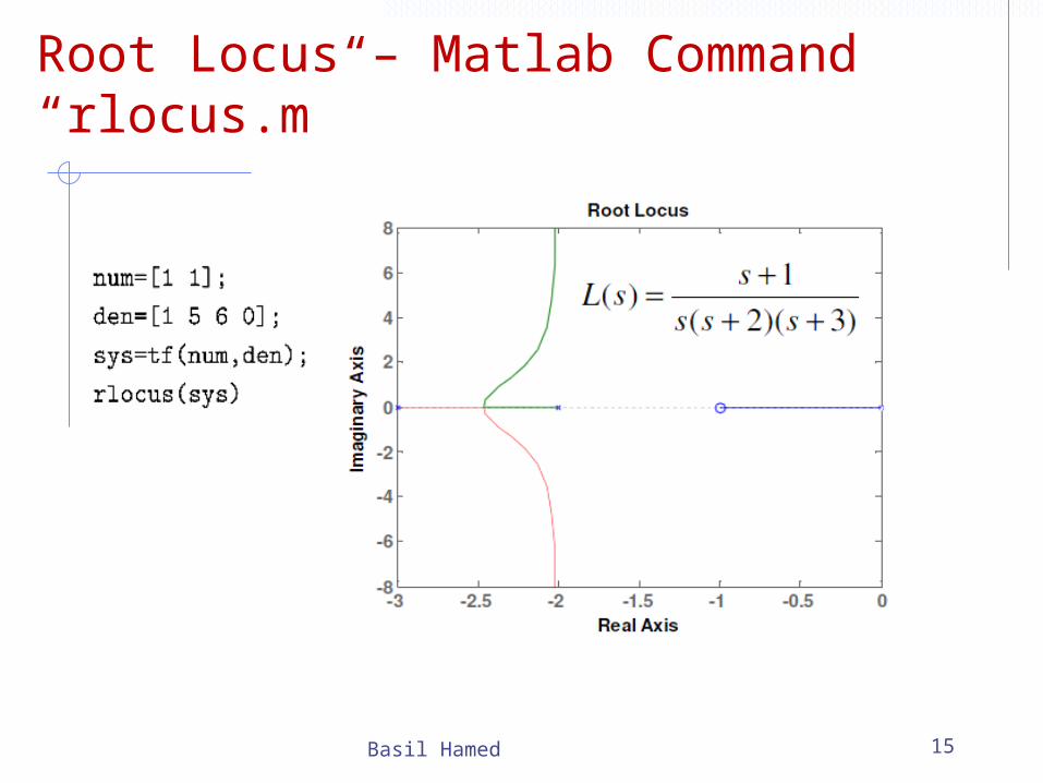
Root Locus – Matlab Command “rlocus.m”

Basil Hamed 15

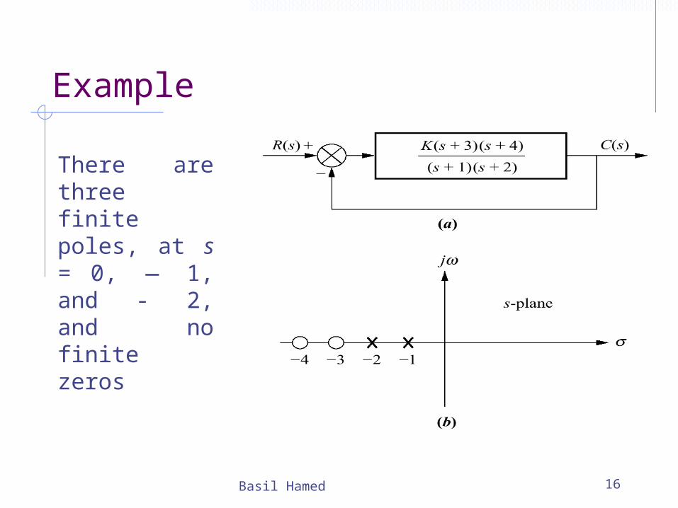
Example

Basil Hamed 16

There are three finite poles, at s = 0, — 1, and - 2, and no finite zeros

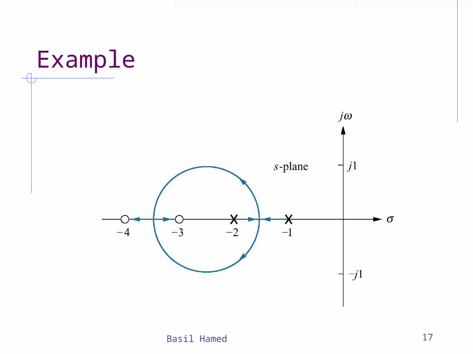
Example

Basil Hamed 17

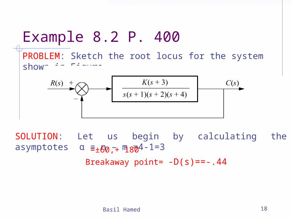
Example 8.2 P. 400PROBLEM: Sketch the root locus for the system shown in Figure

Basil Hamed 18

SOLUTION: Let us begin by calculating the asymptotes α = n – m =4-1=3

=±60,+ 180

Breakaway point= -D(s)==-.44

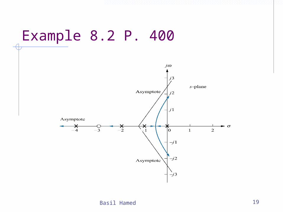
Example 8.2 P. 400

Basil Hamed 19

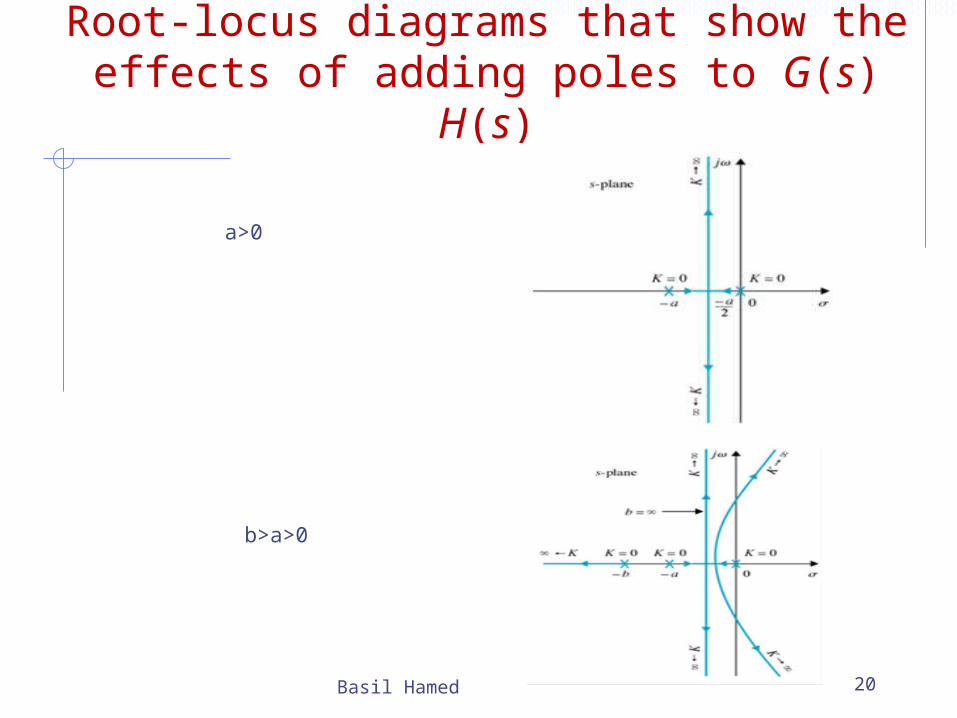
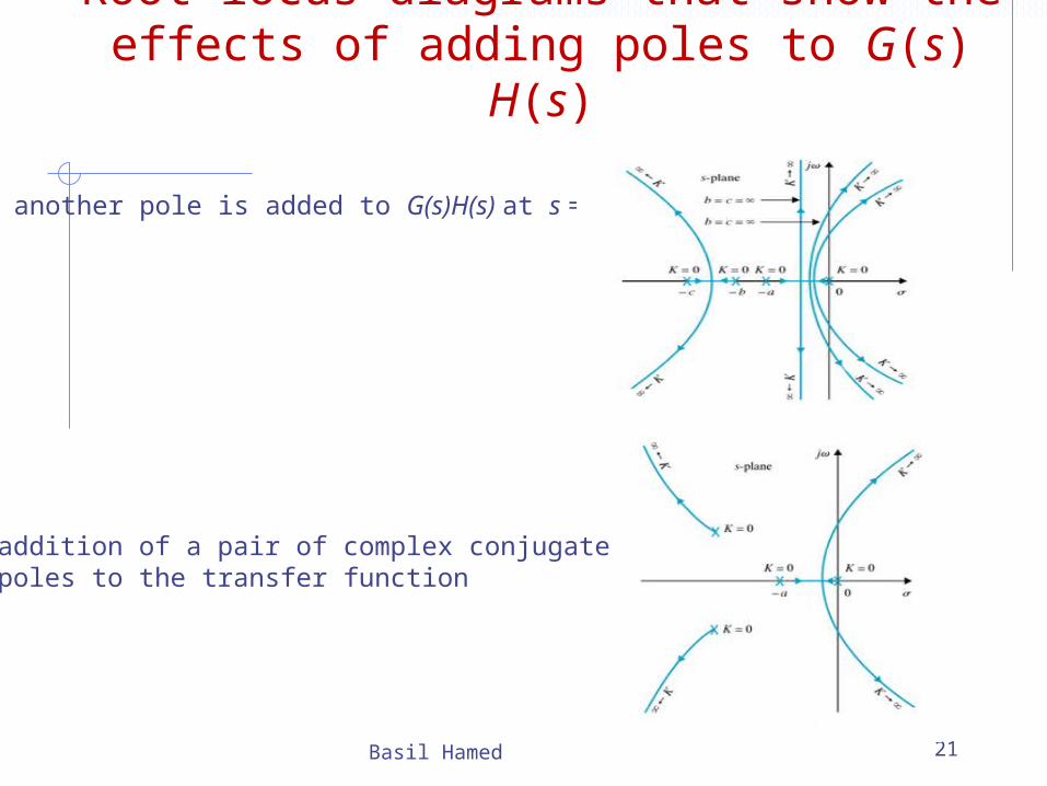
Root-locus diagrams that show the effects of adding poles to G(s) H(s)

Basil Hamed 20

a>0

b>a>0

Root-locus diagrams that show the effects of adding poles to G(s) H(s)

Basil Hamed 21

another pole is added to G(s)H(s) at s = -c

addition of a pair of complex conjugatepoles to the transfer function

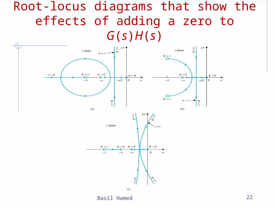
Root-locus diagrams that show the effects of adding a zero to G(s)H(s)

Basil Hamed 22

Example

Given : find R-L when b=1,i) a=10, ii)a=9, iii)a=8 , iv) a=3, v) a=1

Solution: i)a = 10. Breakaway points: s = -2.5 and -4.0.

Basil Hamed 23

Example

Basil Hamed 24

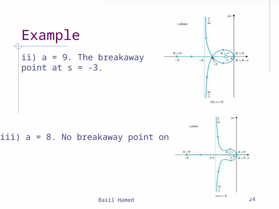
ii) a = 9. The breakaway point at s = -3.

iii) a = 8. No breakaway point on RL

Example

Basil Hamed 25

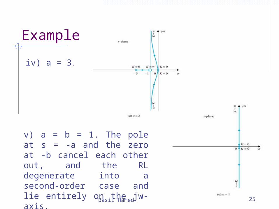
iv) a = 3.

v) a = b = 1. The pole at s = -a and the zero at -b cancel each other out, and the RL degenerate into a second-order case and lie entirely on the jw-axis.

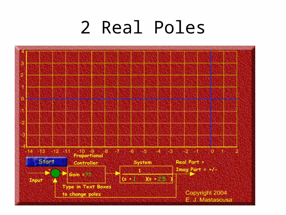
2 Real Poles

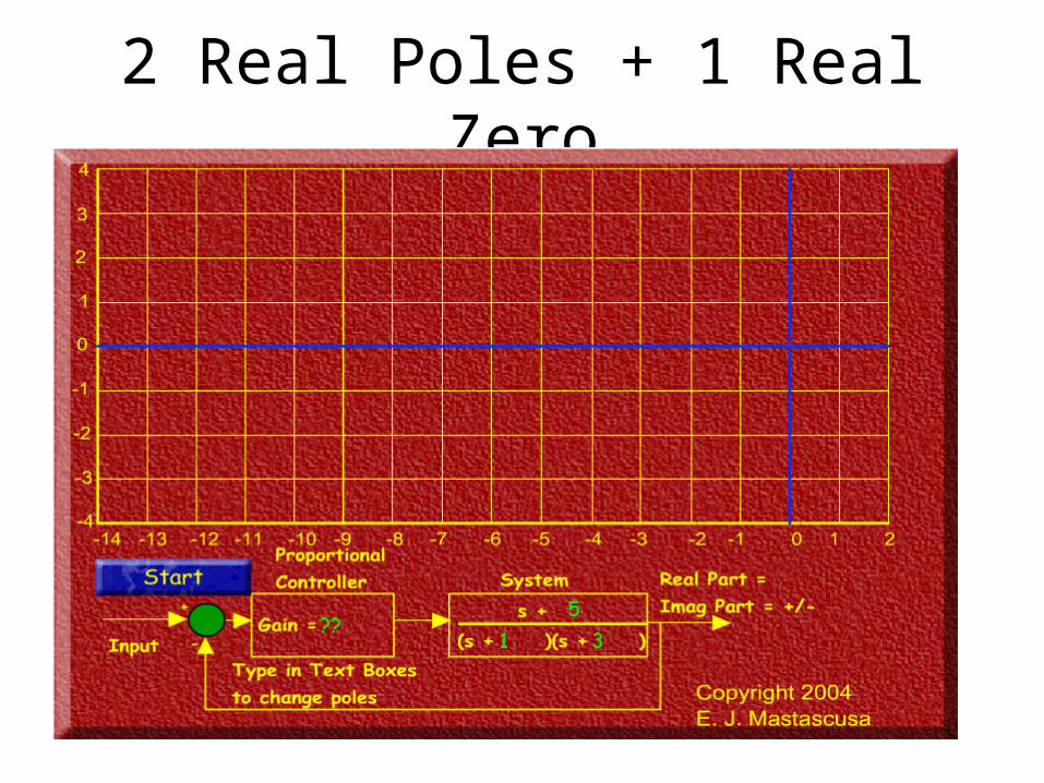
2 Real Poles + 1 Real Zero

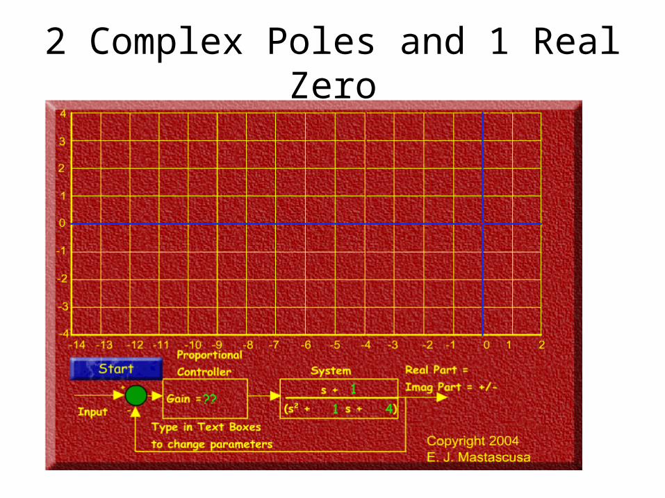
2 Complex Poles and 1 Real Zero

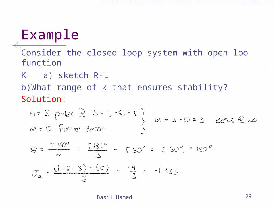
ExampleConsider the closed loop system with open loo function

K a) sketch R-Lb)What range of k that ensures stability?Solution:

Basil Hamed 29

Example

Basil Hamed 30

Not valid

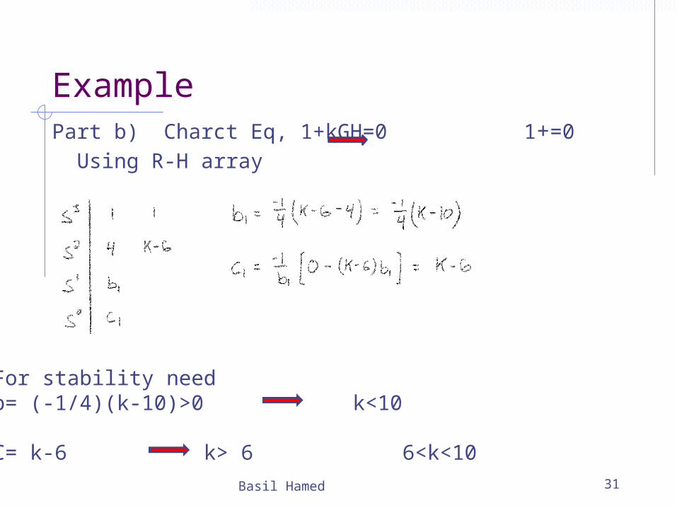
ExamplePart b) Charct Eq, 1+kGH=0 1+=0 Using R-H array

Basil Hamed 31

For stability needb= (-1/4)(k-10)>0 k<10

C= k-6 k> 6 6<k<10

Example

Basil Hamed 32

Find R-L and find k for critical stability

Solution

Breakaway points are among roots of

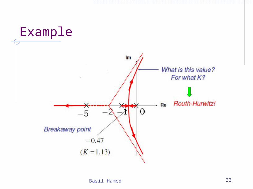
Example

Basil Hamed 33

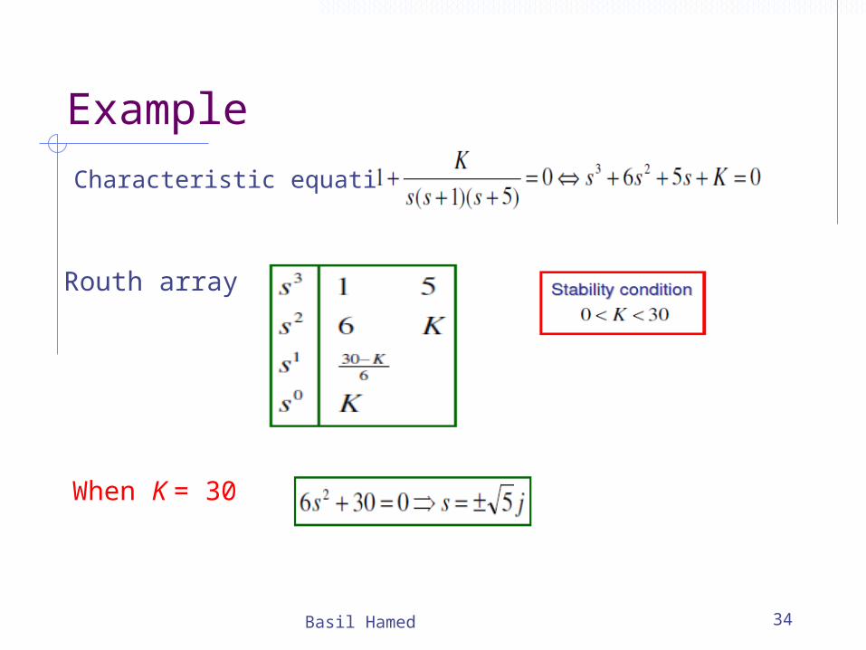
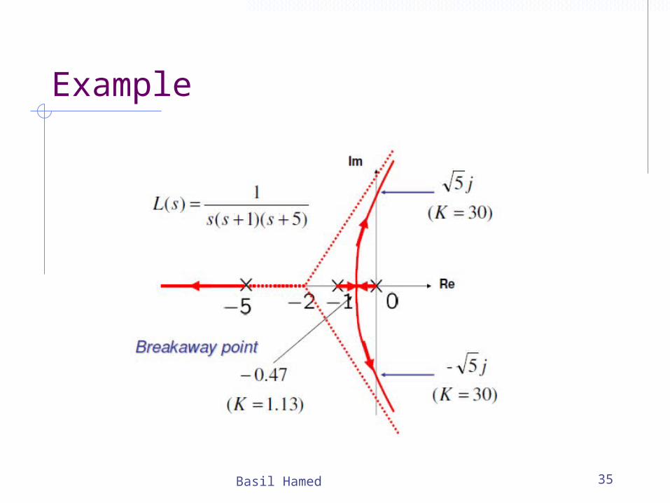
Example

Characteristic equation

Basil Hamed 34

Routh array

When K = 30

Example

Basil Hamed 35

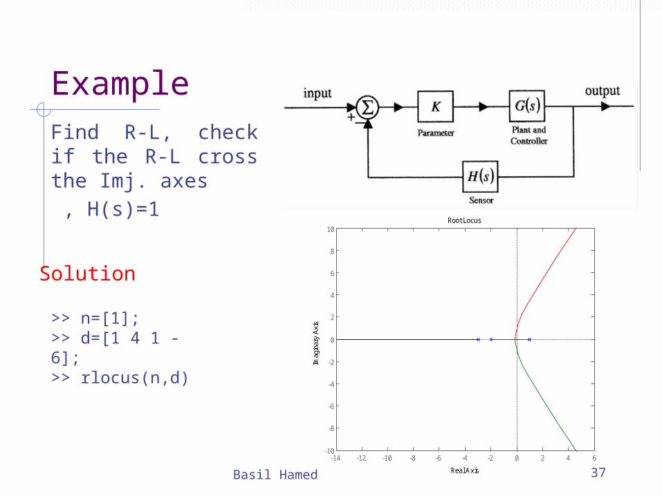
ExampleFind R-L, check if the R-L cross the Imj. axes , H(s)=1

Basil Hamed 36

Solution

-4.5 -4 -3.5 -3 -2.5 -2 -1.5 -1 -0.5 0 0.5-10

-8

-6

-4

-2

0

2

4

6

8

10Root Locus

Real Axis

Imag

inar

y A

xis

>> n=[1 1];>> d=[1 4 0 0];>> rlocus(n,d)

There is no Imj axes crossing

Example

Basil Hamed 37

Find R-L, check if the R-L cross the Imj. axes , H(s)=1

-14 -12 -10 -8 -6 -4 -2 0 2 4 6-10

-8

-6

-4

-2

0

2

4

6

8

10Root Locus

Real Axis

Imag

inar

y A

xis>> n=[1];

>> d=[1 4 1 -6];>> rlocus(n,d)

Solution

Example

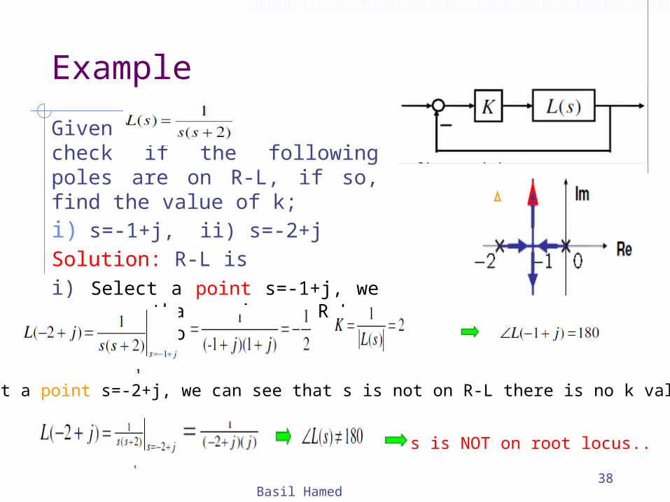
Given check if the following poles are on R-L, if so, find the value of k;i) s=-1+j, ii) s=-2+jSolution: R-L isi) Select a point s=-1+j, we can see that s is on R-L , find value of k

Basil Hamed38

ii) Select a point s=-2+j, we can see that s is not on R-L there is no k value.

s is NOT on root locus..

Example

Basil Hamed 39

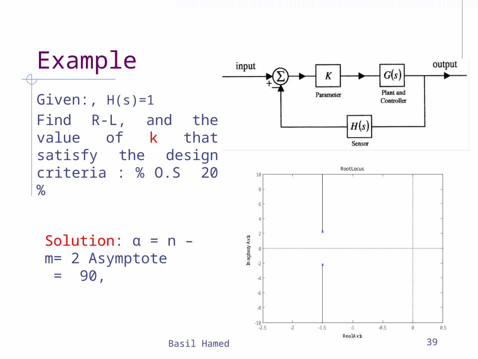
Given:, H(s)=1

Find R-L, and the value of k that satisfy the design criteria : % O.S 20 %

Solution: α = n – m= 2 Asymptote = 90,

-2.5 -2 -1.5 -1 -0.5 0 0.5-10

-8

-6

-4

-2

0

2

4

6

8

10Root Locus

Real Axis

Imag

inar

y A

xis

ExampleFrom % O.S we find ζ=0.45. We have = 2.7 = 3.29, the pole location will be = -1.5 j 2.93. as we can see that the pole will be on the R-L.

The value of k will be =0.382

Basil Hamed 40

Example

Basil Hamed 41

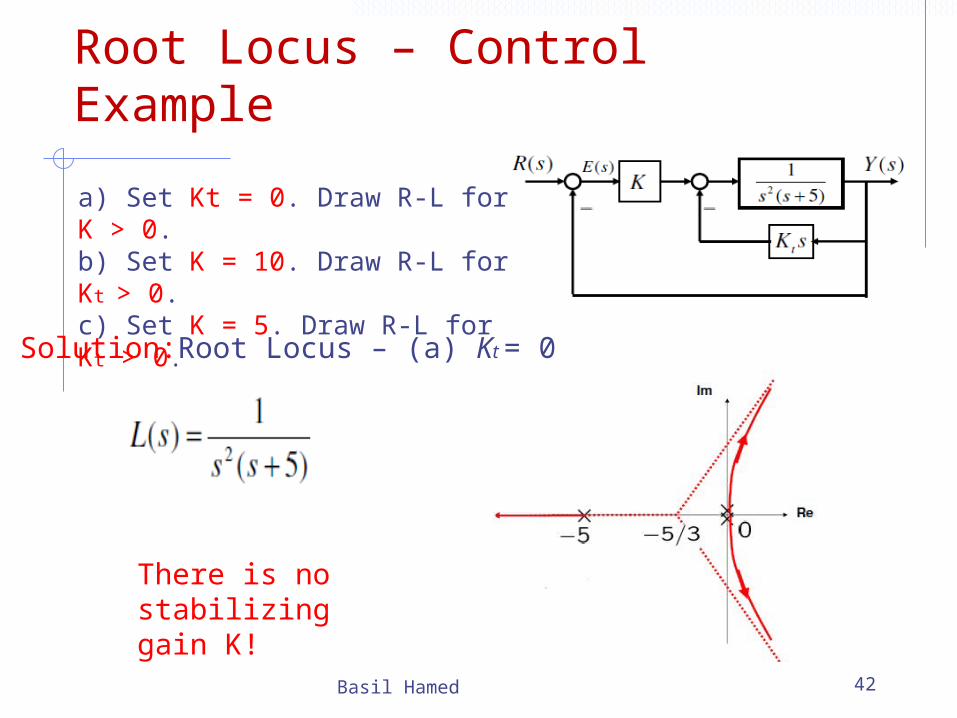
Root Locus – Control Example

Basil Hamed 42

a) Set Kt = 0. Draw R-L for K > 0.b) Set K = 10. Draw R-L for Kt > 0.c) Set K = 5. Draw R-L for Kt > 0.

Solution:Root Locus – (a) Kt = 0

There is nostabilizing gain K!

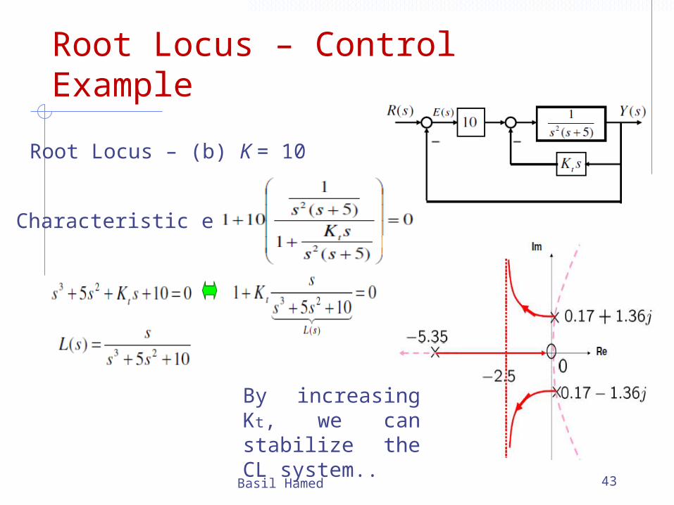
Root Locus – Control Example

Basil Hamed 43

Root Locus – (b) K = 10

Characteristic eq.

By increasing Kt, we can stabilize the CL system..

Root Locus – Control Example

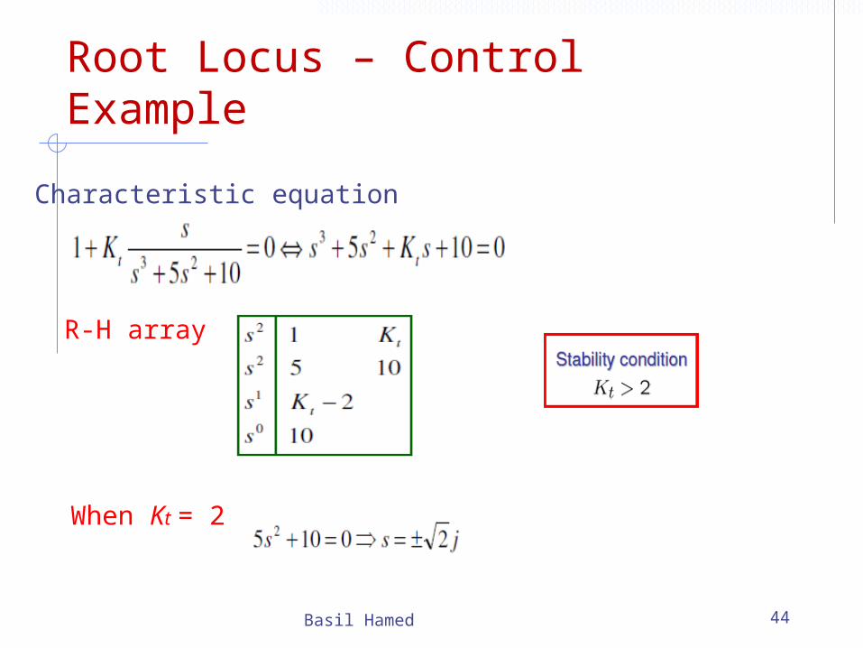
Basil Hamed 44

Characteristic equation

R-H array

When Kt = 2

Root Locus – Control Example

Basil Hamed 45

Root Locus – (c) K = 5

Characteristic eq.

-6 -5 -4 -3 -2 -1 0 1-10

-8

-6

-4

-2

0

2

4

6

8

10Root Locus

Real Axis

Imagin

ary

Axis

>> n=[1 0];>> d=[1 5 0 5];>> rlocus(n,d)

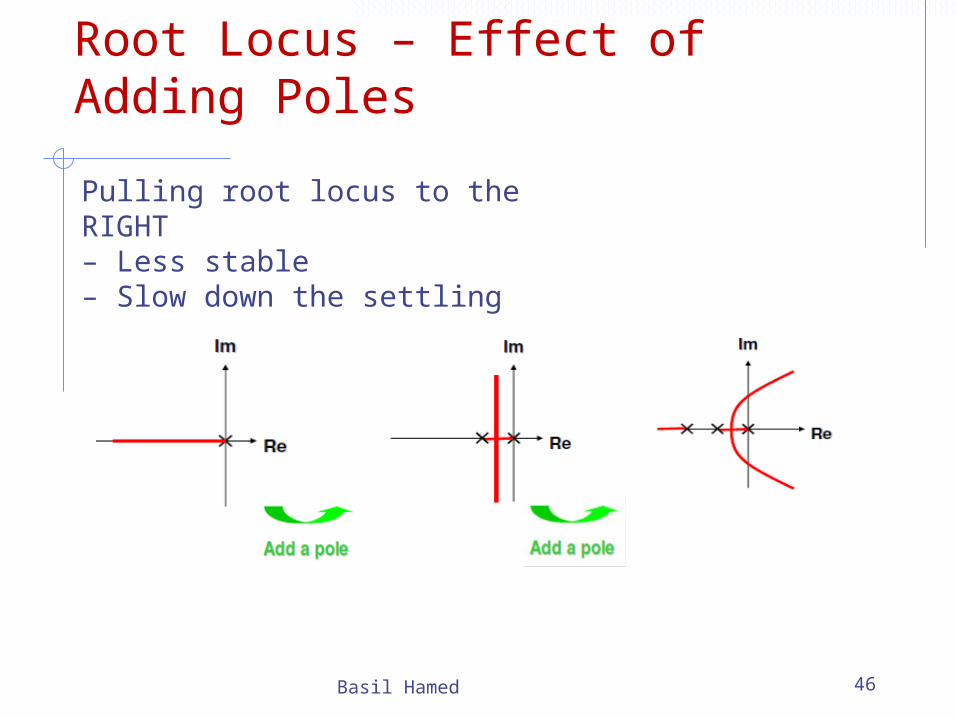
Root Locus – Effect of Adding Poles

Basil Hamed 46

Pulling root locus to the RIGHT– Less stable– Slow down the settling

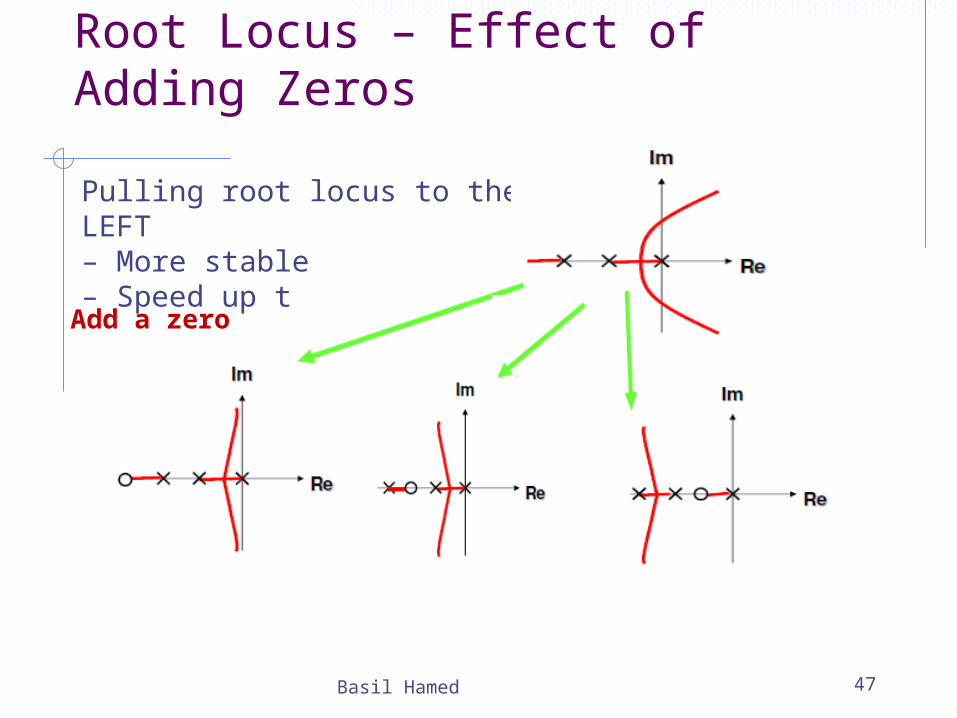
Root Locus – Effect of Adding Zeros

Basil Hamed 47

Pulling root locus to the LEFT– More stable– Speed up the settling

Add a zero

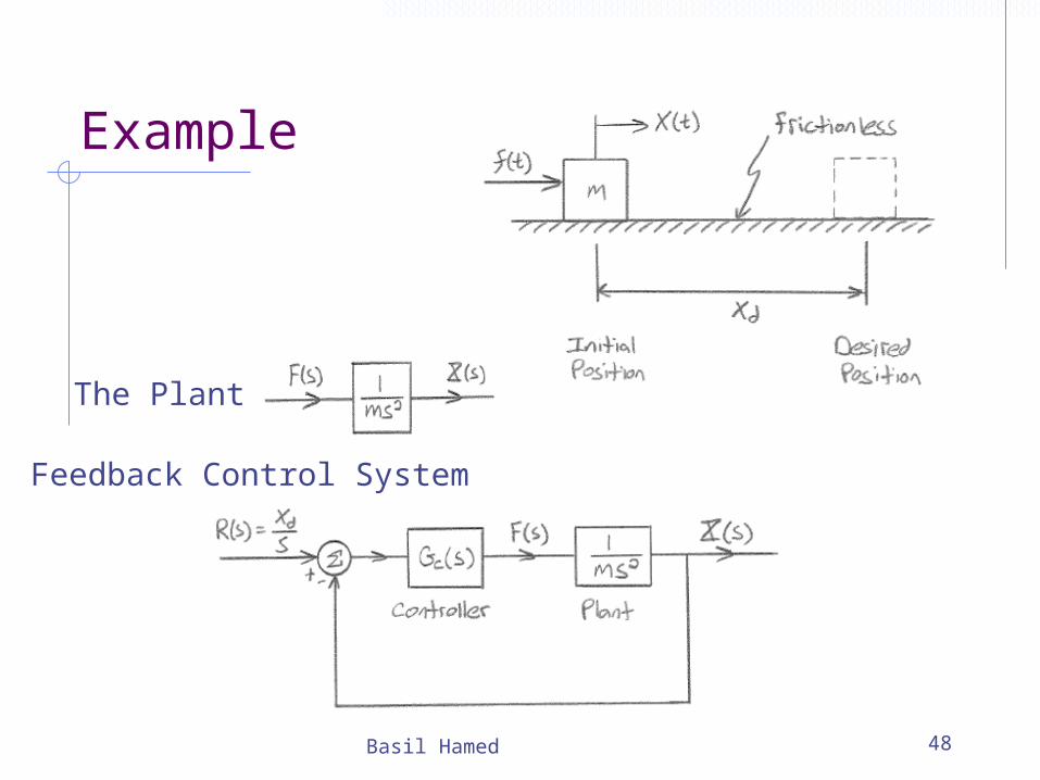
Example

Basil Hamed 48

The Plant

Feedback Control System

ExampleP controller set Gc(s)=k, open loop TF is: Breakaway point=0

Basil Hamed 49

-0.2 -0.15 -0.1 -0.05 0 0.05 0.1 0.15-1.5

-1

-0.5

0

0.5

1

1.5Root Locus

Real Axis

Imagin

ary

Axi

s

>> n=[1];>> d=[1 0 0];>> rlocus(n,d)

Marginal stable for all value of kP control is unacceptable