control systems design - newcastlejhb519/teaching/elec4410/lectures/lec20.… · control systems...
TRANSCRIPT

The University of Newcastle
ELEC4410
Control Systems Design
Lecture 20: Scaling and MIMO State Feedback Design
Julio H. Braslavsky
School of Electrical Engineering and Computer Science
The University of Newcastle
Lecture 20: MIMO State Feedback Design – p. 1

The University of Newcastle
Outline
A Note about Scaling
MIMO State Feedback Design
Cyclic Design
MIMO Regulation and Tracking
MIMO Observers
Lecture 20: MIMO State Feedback Design – p. 2
The University of Newcastle
A Note About Scaling
State space is the preferred model for LTI systems, especially
with higher order models. However, even with state-space
models, accurate results are not guaranteed, because of
the finite-word-length arithmetic of the computer.
Lecture 20: MIMO State Feedback Design – p. 3

The University of Newcastle
A Note About Scaling
State space is the preferred model for LTI systems, especially
with higher order models. However, even with state-space
models, accurate results are not guaranteed, because of
the finite-word-length arithmetic of the computer.
When calculations are performed in a computer, each
arithmetic operation is affected by roundoff error, since
machine hardware can only represent a subset of the real
numbers.
Lecture 20: MIMO State Feedback Design – p. 3

The University of Newcastle
A Note about Scaling
Normalisation:
A well-conditioned problem is usually a prerequisite for obtain-
ing accurate results. One should generally normalize or scale the
matrices (A, B, C, D) of a system to improve their numerical con-
ditioning.
Lecture 20: MIMO State Feedback Design – p. 4
The University of Newcastle
A Note about Scaling
Normalisation:
A well-conditioned problem is usually a prerequisite for obtain-
ing accurate results. One should generally normalize or scale the
matrices (A, B, C, D) of a system to improve their numerical con-
ditioning.
Normalization also allows meaningful statements to be made
about the degree of controllability and observability of the
various inputs and outputs.
Lecture 20: MIMO State Feedback Design – p. 4

The University of Newcastle
A Note about Scaling
A set of matrices (A, B, C, D) can be normalized using diagonal
scaling matrices Nu, Nx and Ny to scale u, x, and y,
u = Nu un, x = Nx x, y = Ny yn
so that the normalised system is
xn = Anxn + Bnun
yn = Cnxn + Dnun
whereAn = N−1
x ANx, Bn = N−1x BNu
Cn = N−1y CNx, Dn = N−1
y DNu
One criterion for the normalisation is to use the maximum
expected range of each of the input, state, and output
variables, e.g., say ±10 Volts.
If possible, choose scaling based upon physical insight to the
problem at hand.
Lecture 20: MIMO State Feedback Design – p. 5
The University of Newcastle
A Note about Scaling
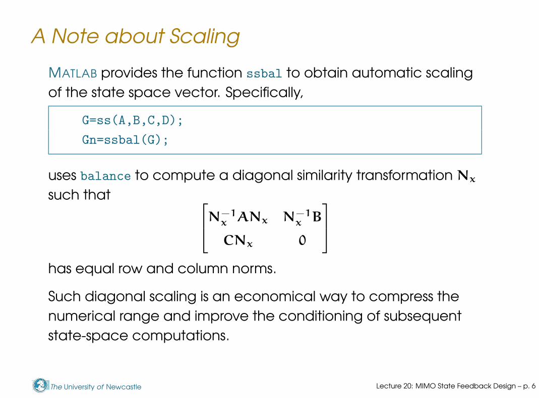
MATLAB provides the function ssbal to obtain automatic scaling
of the state space vector. Specifically,
G=ss(A,B,C,D);
Gn=ssbal(G);
uses balance to compute a diagonal similarity transformation Nx
such that
N−1x ANx N−1
x B
CNx 0
has equal row and column norms.
Such diagonal scaling is an economical way to compress the
numerical range and improve the conditioning of subsequent
state-space computations.
Lecture 20: MIMO State Feedback Design – p. 6
The University of Newcastle
A Note about Scaling
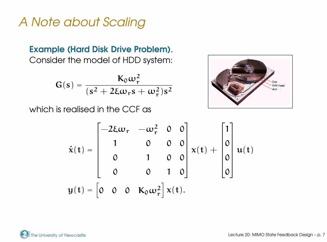
Example (Hard Disk Drive Problem).
Consider the model of HDD system:
G(s) =K0ω2
r
(s2 + 2ξωrs + ω2r)s2
which is realised in the CCF as
x(t) =
−2ξωr −ω2r 0 0
1 0 0 0
0 1 0 0
0 0 1 0
x(t) +
1
0
0
0
u(t)
y(t) =[
0 0 0 K0ω2r
]
x(t).
Lecture 20: MIMO State Feedback Design – p. 7

The University of Newcastle
A Note about Scaling
Data from a real HDD give the parameters
K0 = 1.507 × 10⁴, ξ = 0.1, ωr = 2π × 3400.
With these parameters the matrices in CCF are numerically
ill-conditioned, and MATLAB yields for the controllability matrix
>> rank(ctrb(A,B))
ans = 2
although the realisation is controllable by definition.
Scaling with MATLAB function ssbal gives the correct answer:
>> G=ss(A,B,C,D);
>> Gn=ssbal(G);
>> rank(ctrb(Gn.a,Gn.b))
ans = 4
Lecture 20: MIMO State Feedback Design – p. 8
The University of Newcastle
A Note about Scaling
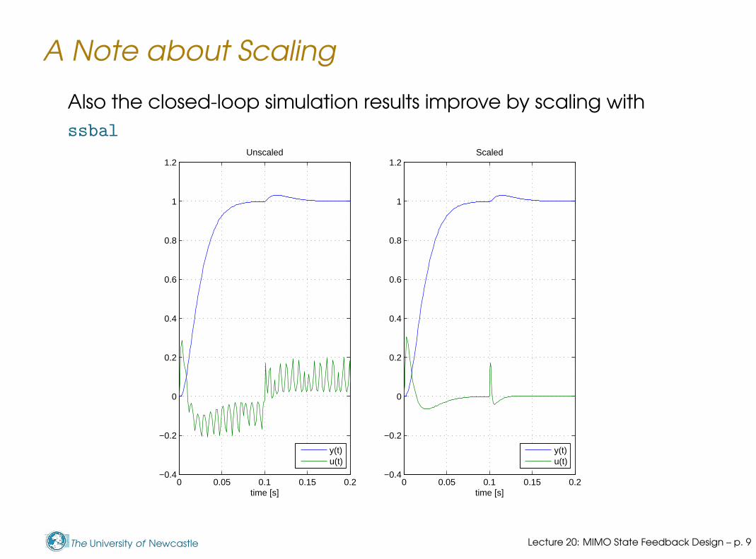
Also the closed-loop simulation results improve by scaling with
ssbal
0 0.05 0.1 0.15 0.2−0.4
−0.2
0
0.2
0.4
0.6
0.8
1
1.2
time [s]
Unscaled
y(t)u(t)
0 0.05 0.1 0.15 0.2−0.4
−0.2
0
0.2
0.4
0.6
0.8
1
1.2
time [s]
Scaled
y(t)u(t)
Lecture 20: MIMO State Feedback Design – p. 9

The University of Newcastle
Outline
A Note about Scaling
MIMO State Feedback Design
Cyclic Design
MIMO Regulation and Tracking
MIMO Observers
Lecture 20: MIMO State Feedback Design – p. 10

The University of Newcastle
MIMO State Feedback Design
We now return to discuss MIMO LTI systems, this time, in the state
space framework.
Recall from Lecture 10 that MIMO systems presented additional
difficulties in the transfer function “language”. The concepts of
poles and zeros were more complicated, and control design,
such as IMC design, turned out to be quite more messier than for
SISO systems, particularly for nonsquare, possibly unstable plants.
The state space representation is particularly suited to MIMO
systems. As we will see, there is no essential difference with the
SISO procedures for state space control and observer design,
even when the plant is nonsquare.
Lecture 20: MIMO State Feedback Design – p. 11

The University of Newcastle
MIMO State Feedback Design
Before entering into the design methods, let’s note that the
results regarding controllability and eigenvalue assignability
extend to the MIMO case.
Lecture 20: MIMO State Feedback Design – p. 12

The University of Newcastle
MIMO State Feedback Design
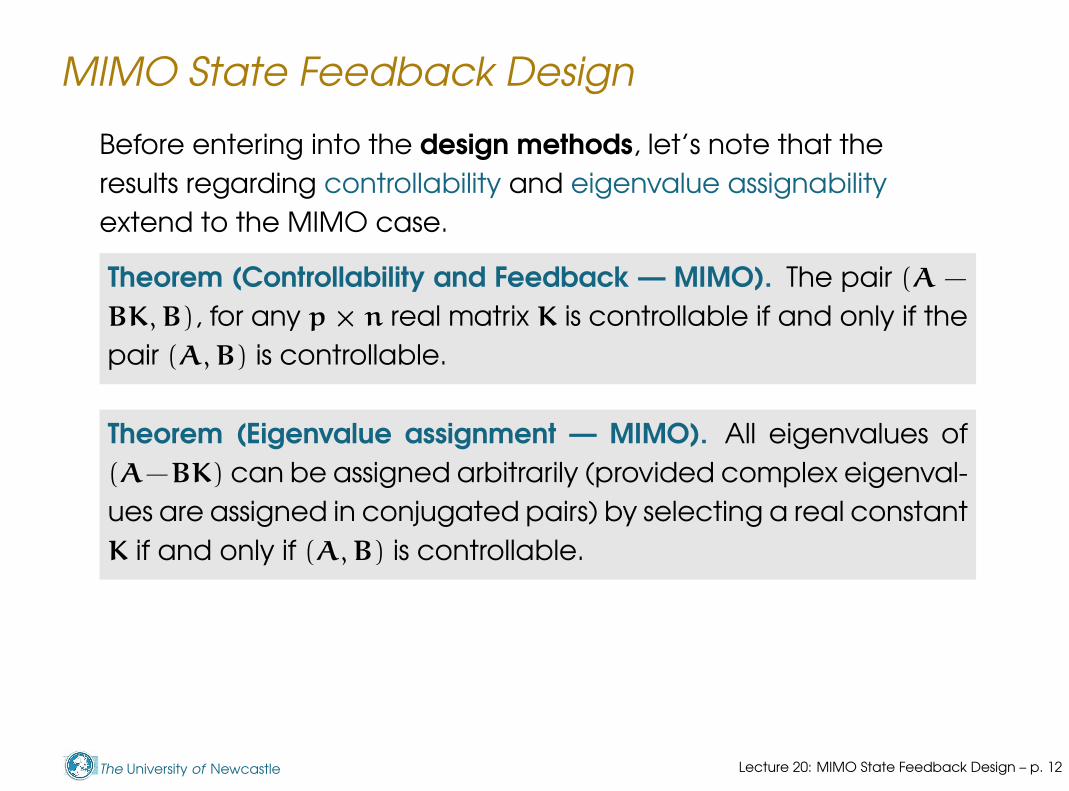
Before entering into the design methods, let’s note that the
results regarding controllability and eigenvalue assignability
extend to the MIMO case.
Theorem (Controllability and Feedback — MIMO). The pair (A −
BK, B), for any p × n real matrix K is controllable if and only if the
pair (A, B) is controllable.
Lecture 20: MIMO State Feedback Design – p. 12
The University of Newcastle
MIMO State Feedback Design
Before entering into the design methods, let’s note that the
results regarding controllability and eigenvalue assignability
extend to the MIMO case.
Theorem (Controllability and Feedback — MIMO). The pair (A −
BK, B), for any p × n real matrix K is controllable if and only if the
pair (A, B) is controllable.
Theorem (Eigenvalue assignment — MIMO). All eigenvalues of
(A−BK) can be assigned arbitrarily (provided complex eigenval-
ues are assigned in conjugated pairs) by selecting a real constant
K if and only if (A, B) is controllable.
Lecture 20: MIMO State Feedback Design – p. 12

The University of Newcastle
MIMO State Feedback Design
A MIMO system in state space is described with the same
formalism we have been using for SISO systems, i.e.,
x(t) = Ax(t) + Bu(t) x ∈ Rn, u ∈ R
p
y(t) = Cx(t) y ∈ Rq
When the system has p inputs, the state feedback gain K in a
feedback law
u = −Kx = −
k11 k12 ··· k1n
k21 k22 ··· k2n
...... ···
...kp1 kp2 ··· kpn
x1x2
...xn
will have p × n parameters. That is, K ∈ Rp×n.
Lecture 20: MIMO State Feedback Design – p. 13

The University of Newcastle
MIMO State Feedback Design
A MIMO system in state space is described with the same
formalism we have been using for SISO systems, i.e.,
x(t) = Ax(t) + Bu(t) x ∈ Rn, u ∈ R
p
y(t) = Cx(t) y ∈ Rq
When the system has p inputs, the state feedback gain K in a
feedback law
u = −Kx = −p
{
k11 k12 ··· k1n
k21 k22 ··· k2n
...... ···
...kp1 kp2 ··· kpn
x1x2
...xn
}
n
will have p × n parameters. That is, K ∈ Rp×n.
Lecture 20: MIMO State Feedback Design – p. 13
The University of Newcastle
MIMO State Feedback Design
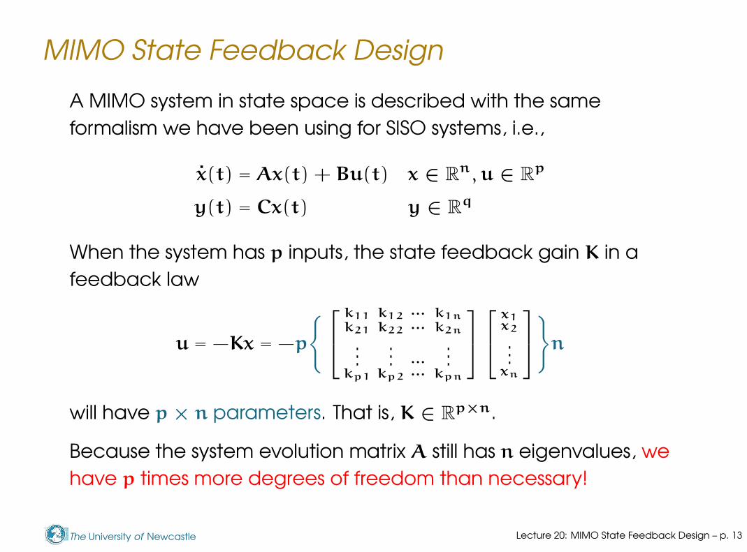
A MIMO system in state space is described with the same
formalism we have been using for SISO systems, i.e.,
x(t) = Ax(t) + Bu(t) x ∈ Rn, u ∈ R
p
y(t) = Cx(t) y ∈ Rq
When the system has p inputs, the state feedback gain K in a
feedback law
u = −Kx = −p
{
k11 k12 ··· k1n
k21 k22 ··· k2n
...... ···
...kp1 kp2 ··· kpn
x1x2
...xn
}
n
will have p × n parameters. That is, K ∈ Rp×n.
Because the system evolution matrix A still has n eigenvalues, we
have p times more degrees of freedom than necessary!
Lecture 20: MIMO State Feedback Design – p. 13

The University of Newcastle
MIMO State Feedback Design
Example (Nonuniqueness of K in MIMO state feedback). As a
simple MIMO system consider the second order system with two
inputs
x(t) =
0 0
1 0
x(t) +
1 0
0 1
u(t)
The system has two eigenvalues at s = 0, and it is controllable,
since B = I, so C = [ B AB ] is full rank.
Let’s consider the state feedback
u(t) = −Kx(t) =[
k11 k12
k21 k22
]
x(t)
Then the closed loop evolution matrix is
A − BK =[
−k11 −k12
1−k21 −k22
]
Lecture 20: MIMO State Feedback Design – p. 14
The University of Newcastle
MIMO State Feedback Design
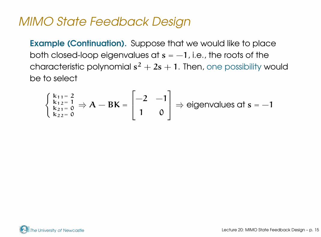
Example (Continuation). Suppose that we would like to place
both closed-loop eigenvalues at s = −1, i.e., the roots of the
characteristic polynomial s2 + 2s + 1. Then, one possibility would
be to select
{k11= 2k12= 1k21= 0k22= 0
⇒ A − BK =
−2 −1
1 0
⇒ eigenvalues at s = −1
Lecture 20: MIMO State Feedback Design – p. 15
The University of Newcastle
MIMO State Feedback Design
Example (Continuation). Suppose that we would like to place
both closed-loop eigenvalues at s = −1, i.e., the roots of the
characteristic polynomial s2 + 2s + 1. Then, one possibility would
be to select
{k11= 2k12= 1k21= 0k22= 0
⇒ A − BK =
−2 −1
1 0
⇒ eigenvalues at s = −1
But the alternative selection
{k11= 1k12= freek21= 1k22= −1
⇒ A − BK =
−1 k12
0 −1
⇒ also eigenvalues at s = −1
Lecture 20: MIMO State Feedback Design – p. 15

The University of Newcastle
MIMO State Feedback Design
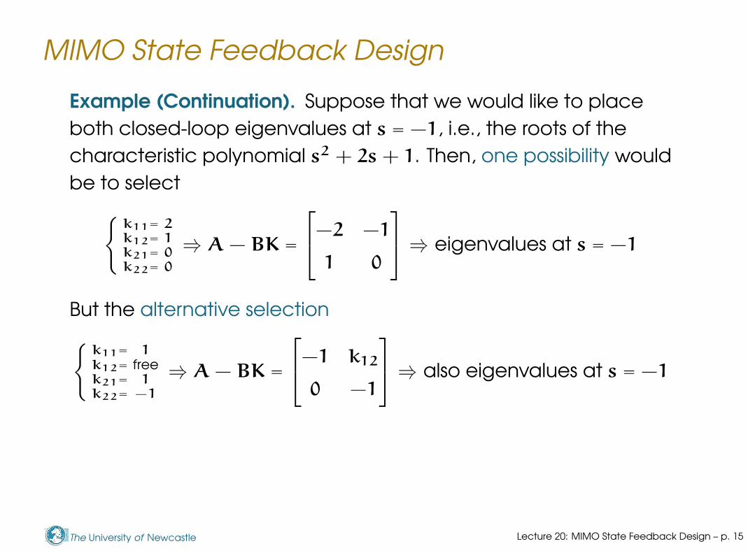
Example (Continuation). Suppose that we would like to place
both closed-loop eigenvalues at s = −1, i.e., the roots of the
characteristic polynomial s2 + 2s + 1. Then, one possibility would
be to select
{k11= 2k12= 1k21= 0k22= 0
⇒ A − BK =
−2 −1
1 0
⇒ eigenvalues at s = −1
But the alternative selection
{k11= 1k12= freek21= 1k22= −1
⇒ A − BK =
−1 k12
0 −1
⇒ also eigenvalues at s = −1
As we see, there are infinitely many possible selections of K that
will give the same eigenvalues of (A − BK)!
Lecture 20: MIMO State Feedback Design – p. 15

The University of Newcastle
MIMO State Feedback Design
The “excess of freedom” in MIMO state feedback design could
be a problem if we don’t know how to best use it. . .
There are several ways to tackle the problem of selecting K from
an infinite number of possibilities, among them
Cyclic Design. Reduces the problem to one of a single input,
so we can apply the known rules.
Lecture 20: MIMO State Feedback Design – p. 16

The University of Newcastle
MIMO State Feedback Design
The “excess of freedom” in MIMO state feedback design could
be a problem if we don’t know how to best use it. . .
There are several ways to tackle the problem of selecting K from
an infinite number of possibilities, among them
Cyclic Design. Reduces the problem to one of a single input,
so we can apply the known rules.
Controller Canonical Form Design. Extends the Bass-Gura
formula to MIMO.
Optimal Design. Computes the best K by optimising a
suitable cost function.
We will discuss the Cyclic and Optimal designs.
Lecture 20: MIMO State Feedback Design – p. 16

The University of Newcastle
Outline
A Note about Scaling
MIMO State Feedback Design
Cyclic Design
MIMO Regulation and Tracking
MIMO Observers
Lecture 20: MIMO State Feedback Design – p. 17

The University of Newcastle
MIMO Cyclic State Feedback Design
MIMO Cyclic Design. In this design we change the multi-input
problem into a single-input problem by creating a new input that
is a linear combination of the inputs to the plant. This technique
relies on the fact that
If a state equation can be controlled by many inputs, then it can
be controlled by one input.
+B1 B2 B3
∫
A
C1
C3
C2
Lecture 20: MIMO State Feedback Design – p. 18
The University of Newcastle
MIMO Cyclic State Feedback Design
MIMO Cyclic Design. In this design we change the multi-input
problem into a single-input problem by creating a new input that
is a linear combination of the inputs to the plant. This technique
relies on the fact that
If a state equation can be controlled by many inputs, then it can
be controlled by one input.
+
v1
v2
v3
B1 B2 B3
∫
A
C1
C3
C2
Lecture 20: MIMO State Feedback Design – p. 18

The University of Newcastle
MIMO Cyclic State Feedback Design
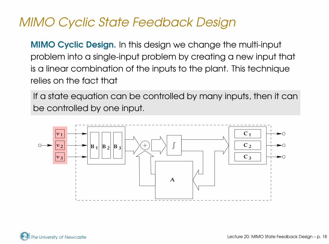
MIMO Cyclic Design. In this design we change the multi-input
problem into a single-input problem by creating a new input that
is a linear combination of the inputs to the plant. This technique
relies on the fact that
If a state equation can be controlled by many inputs, then it can
be controlled by one input.
+
v1
v2
v3
B1 B2 B3
∫
A
C1
C3
C2
We need to define the minimal polynomial of a matrix, and
what a cyclic matrix is, before proceeding with this technique.
Lecture 20: MIMO State Feedback Design – p. 18

The University of Newcastle
MIMO Cyclic State Feedback Design
Recall that by the Cayley Hamilton Theorem, every matrix
satisfies its characteristic polynomial, i.e.,
if ∆(s) = det(sI − A) = sn + α1sn−1 + · · · + α0,
then An + α1An−1 + · · · + α0I = 0.
Lecture 20: MIMO State Feedback Design – p. 19

The University of Newcastle
MIMO Cyclic State Feedback Design
Recall that by the Cayley Hamilton Theorem, every matrix
satisfies its characteristic polynomial, i.e.,
if ∆(s) = det(sI − A) = sn + α1sn−1 + · · · + α0,
then An + α1An−1 + · · · + α0I = 0.
But the characteristic polynomial is not necessarily the smallest
degree monic polynomial a matrix may satisfy. That polynomial
is called the minimal polynomial of a matrix.
Lecture 20: MIMO State Feedback Design – p. 19

The University of Newcastle
MIMO Cyclic State Feedback Design
Example (Minimal Polynomial of a Matrix). The characteristic
polynomial of the matrix
A =[
−1 0 00 −1 00 0 2
]
is ∆(s) = (s + 1)2(s + 2) = s3 + 4s2 + 5s + 2
Thus
A3 + 4A2 + 5A + 2I = 0.
But it could be verified that A also satisfies
∆m(s) = (s + 1)(s + 2) = s2 + 3s + 2,
which is the smallest degree monic polynomial A satisfies. That is
the minimal polynomial of A.
Lecture 20: MIMO State Feedback Design – p. 20

The University of Newcastle
MIMO Cyclic State Feedback Design
A matrix A is cyclic if its characteristic polynomial equals its mini-
mal polynomial.
Lecture 20: MIMO State Feedback Design – p. 21
The University of Newcastle
MIMO Cyclic State Feedback Design
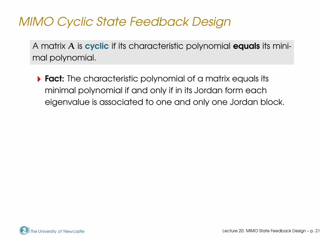
A matrix A is cyclic if its characteristic polynomial equals its mini-
mal polynomial.
Fact: The characteristic polynomial of a matrix equals its
minimal polynomial if and only if in its Jordan form each
eigenvalue is associated to one and only one Jordan block.
Lecture 20: MIMO State Feedback Design – p. 21
The University of Newcastle
MIMO Cyclic State Feedback Design
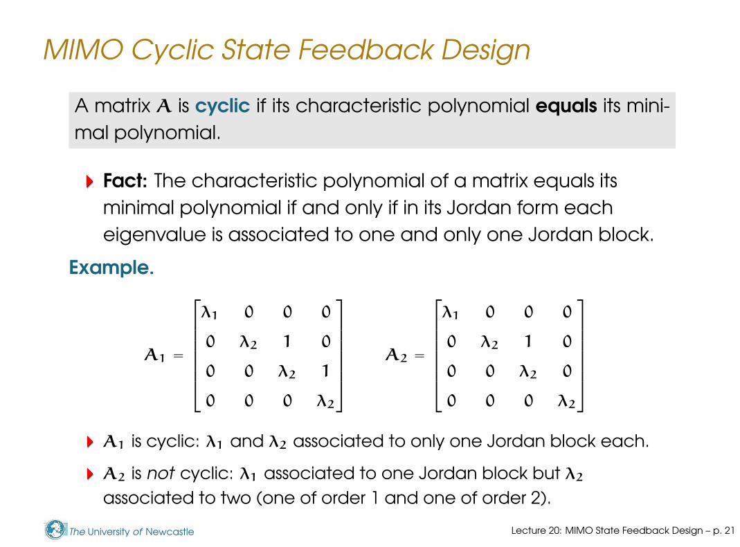
A matrix A is cyclic if its characteristic polynomial equals its mini-
mal polynomial.
Fact: The characteristic polynomial of a matrix equals its
minimal polynomial if and only if in its Jordan form each
eigenvalue is associated to one and only one Jordan block.
Example.
A1 =
2
6
6
6
6
6
4
λ1 0 0 0
0 λ2 1 0
0 0 λ2 1
0 0 0 λ2
3
7
7
7
7
7
5
A2 =
2
6
6
6
6
6
4
λ1 0 0 0
0 λ2 1 0
0 0 λ2 0
0 0 0 λ2
3
7
7
7
7
7
5
A1 is cyclic: λ1 and λ2 associated to only one Jordan block each.
A2 is not cyclic: λ1 associated to one Jordan block but λ2
associated to two (one of order 1 and one of order 2).
Lecture 20: MIMO State Feedback Design – p. 21

The University of Newcastle
MIMO Cyclic State Feedback Design
Notice that if a matrix has no repeated eigenvalues, then it is
cyclic, since all the eigenvalues will be distinct and necessarily
each associated to just one Jordan block (of order 1).
Lecture 20: MIMO State Feedback Design – p. 22

The University of Newcastle
MIMO Cyclic State Feedback Design
Notice that if a matrix has no repeated eigenvalues, then it is
cyclic, since all the eigenvalues will be distinct and necessarily
each associated to just one Jordan block (of order 1).
Theorem (Controllability with p inputs and controllability with 1 in-
put). If the n-dimensional p-input pair (A, B) is controllable and
if A is cyclic, then for almost any p × 1 vector V, the single-input
pair (A, BV) is controllable.
When we say almost any V, we mean that if we select a V
matrix randomly, there is virtually probability 0 that we will end
up with one that won’t work.
We show intuitively why this is so on an example.
Lecture 20: MIMO State Feedback Design – p. 22

The University of Newcastle
MIMO Cyclic State Feedback Design
Consider the pair (A, B), with 5 states and 2 inputs, defined by
A =
2
6
6
6
6
6
6
6
6
6
6
6
4
2 1 0
0 2 1
0 0 2
0 0
0 0
0 0
0 0 0
0 0 0
1 1
0 1
3
7
7
7
7
7
7
7
7
7
7
7
5
B =
2
6
6
6
6
6
6
6
6
4
0 1
0 0
1 2
4 3
1 0
3
7
7
7
7
7
7
7
7
5
, and let BV = B
2
4
v1
v2
3
5 =
2
6
6
6
6
6
6
6
6
4
∗
∗
α
∗
β
3
7
7
7
7
7
7
7
7
5
.
Notice that A is cyclic, since each of the two distinct
eigenvalues 2 and 1, are associated to one and only one Jordan
block (respectively of orders 3 and 2).
If we pretend to control A with the single input built by the
product BV, then in order to retain controllability we will need
α 6= 0 and β 6= 0.
Lecture 20: MIMO State Feedback Design – p. 23

The University of Newcastle
MIMO Cyclic State Feedback Design
In other words, because
2
6
6
6
6
6
6
6
6
4
∗
∗
α
∗
β
3
7
7
7
7
7
7
7
7
5
= BV =
2
6
6
6
6
6
6
6
6
4
0 1
0 0
1 2
4 3
1 0
3
7
7
7
7
7
7
7
7
5
2
4
v1
v2
3
5 =
2
6
6
6
6
6
6
6
6
4
∗
∗
v1 + 2v2
∗
v1
3
7
7
7
7
7
7
7
7
5
,
controllability with a single input requires 6
-
HHHHHHHH
v2
v11 2
1
2
v1 = −2v2
v1 = 0
v1 + 2v2 6= 0 , and v1 6= 0.
which means that in the (v1, v2) plane we
have to choose a pair (v1, v2)
off the red lines shown in the picture. Almost any
random pair (v1, v2) will satisfy this condition.
Lecture 20: MIMO State Feedback Design – p. 24

The University of Newcastle
MIMO Cyclic State Feedback Design
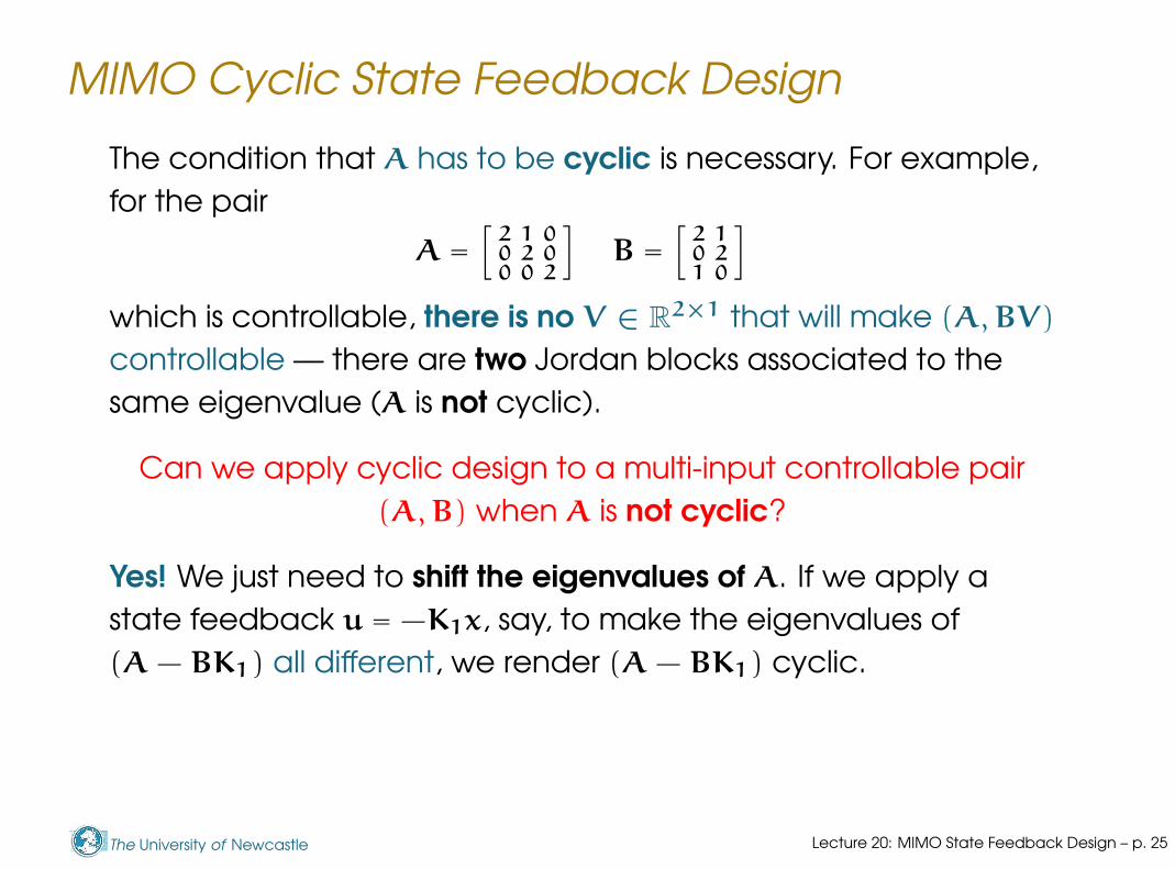
The condition that A has to be cyclic is necessary. For example,
for the pair
A =[
2 1 00 2 00 0 2
]
B =[
2 10 21 0
]
which is controllable, there is no V ∈ R2×1 that will make (A, BV)
controllable — there are two Jordan blocks associated to the
same eigenvalue (A is not cyclic).
Lecture 20: MIMO State Feedback Design – p. 25

The University of Newcastle
MIMO Cyclic State Feedback Design
The condition that A has to be cyclic is necessary. For example,
for the pair
A =[
2 1 00 2 00 0 2
]
B =[
2 10 21 0
]
which is controllable, there is no V ∈ R2×1 that will make (A, BV)
controllable — there are two Jordan blocks associated to the
same eigenvalue (A is not cyclic).
Can we apply cyclic design to a multi-input controllable pair
(A, B) when A is not cyclic?
Lecture 20: MIMO State Feedback Design – p. 25
The University of Newcastle
MIMO Cyclic State Feedback Design
The condition that A has to be cyclic is necessary. For example,
for the pair
A =[
2 1 00 2 00 0 2
]
B =[
2 10 21 0
]
which is controllable, there is no V ∈ R2×1 that will make (A, BV)
controllable — there are two Jordan blocks associated to the
same eigenvalue (A is not cyclic).
Can we apply cyclic design to a multi-input controllable pair
(A, B) when A is not cyclic?
Yes! We just need to shift the eigenvalues of A. If we apply a
state feedback u = −K1x, say, to make the eigenvalues of
(A − BK1) all different, we render (A − BK1) cyclic.
Lecture 20: MIMO State Feedback Design – p. 25

The University of Newcastle
MIMO Cyclic State Feedback Design
Any randomly chosen K1 will generically produce closed-loop
eigenvalues that are all different. We can then apply cyclic
design to the modified pair (A − BK1, BV).
The Cyclic design procedure may be summarised as
Procedure for eigenvalue assignment in multi-input state equa-
tions by cyclic state feedback design.
1. Check controllability of the n-state, p-input pair (A, B).
2. Compute a random state feedback gain K1 ∈ Rp × n. The
matrix (A − BK1) should be cyclic.
3. Compute a random precompensating matrix V ∈ Rp×1. The
single input pair (A − BK1, BV) should be controllable.
4. Find a state feedback gain K2 to place the eigenvalues of
(A − BK1 − BVK2) at the desired locations.
Lecture 20: MIMO State Feedback Design – p. 26

The University of Newcastle
MIMO Cyclic State Feedback Design
In MATLAB, we can use the function rand to generate normally
distributed random gains
[n,p]=size(B);
K1=rand(p,n);
V=rand(p,1);
Once we computed
g bb g g - - -
¾6
¾
6
¾
- - -6
--−−
B∫
A
K1
C
VK2
x x yurK1, V and K2, the
total state feedback law is
u = −Kx, with K = K1 + VK2.
Lecture 20: MIMO State Feedback Design – p. 27

The University of Newcastle
Outline
A Note about Scaling
MIMO State Feedback Design
Cyclic Design
MIMO Regulation and Tracking
MIMO Observers
Lecture 20: MIMO State Feedback Design – p. 28

The University of Newcastle
MIMO Regulation and Tracking
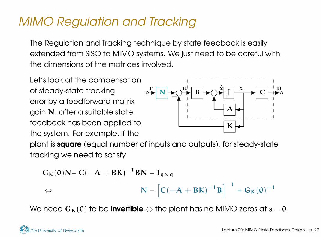
The Regulation and Tracking technique by state feedback is easily
extended from SISO to MIMO systems. We just need to be careful with
the dimensions of the matrices involved.
Lecture 20: MIMO State Feedback Design – p. 29
The University of Newcastle
MIMO Regulation and Tracking
The Regulation and Tracking technique by state feedback is easily
extended from SISO to MIMO systems. We just need to be careful with
the dimensions of the matrices involved.
Let’s look at the compensation
f fb b- - -
¾
¾6
-- -6
-
K
A
∫x xC
yu
−
rBNof steady-state tracking
error by a feedforward matrix
gain N, after a suitable state
feedback has been applied to
the system. For example, if the
plant is square (equal number of inputs and outputs), for steady-state
tracking we need to satisfy
GK(0)N= C(−A + BK)−1
BN = Iq×q
⇔ N =h
C(−A + BK)−1
Bi−1
= GK(0)−1
We need GK(0) to be invertible ⇔ the plant has no MIMO zeros at s = 0.
Lecture 20: MIMO State Feedback Design – p. 29

The University of Newcastle
MIMO Regulation and Tracking
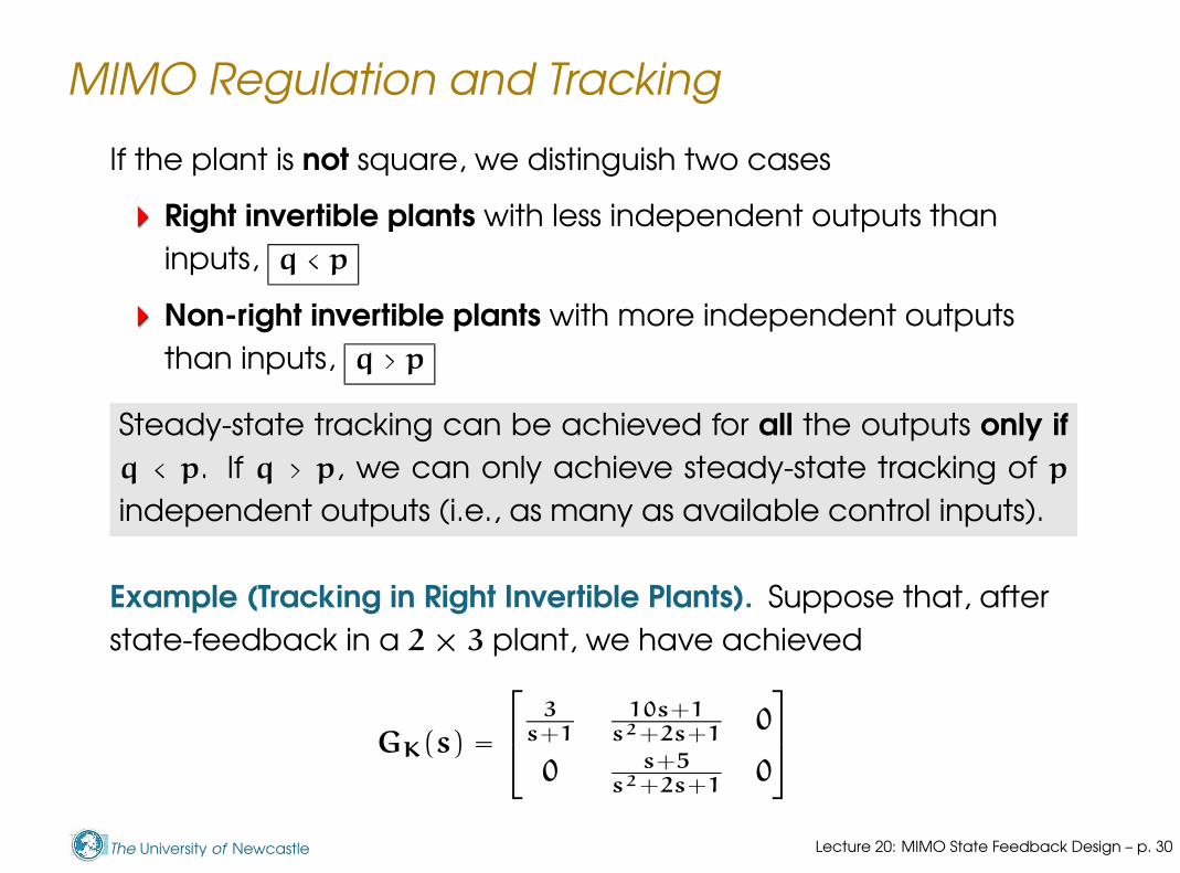
If the plant is not square, we distinguish two cases
Right invertible plants with less independent outputs than
inputs, q < p
Non-right invertible plants with more independent outputs
than inputs, q > p
Lecture 20: MIMO State Feedback Design – p. 30

The University of Newcastle
MIMO Regulation and Tracking
If the plant is not square, we distinguish two cases
Right invertible plants with less independent outputs than
inputs, q < p
Non-right invertible plants with more independent outputs
than inputs, q > p
Steady-state tracking can be achieved for all the outputs only if
q < p. If q > p, we can only achieve steady-state tracking of p
independent outputs (i.e., as many as available control inputs).
Lecture 20: MIMO State Feedback Design – p. 30
The University of Newcastle
MIMO Regulation and Tracking
If the plant is not square, we distinguish two cases
Right invertible plants with less independent outputs than
inputs, q < p
Non-right invertible plants with more independent outputs
than inputs, q > p
Steady-state tracking can be achieved for all the outputs only if
q < p. If q > p, we can only achieve steady-state tracking of p
independent outputs (i.e., as many as available control inputs).
Example (Tracking in Right Invertible Plants). Suppose that, after
state-feedback in a 2 × 3 plant, we have achieved
GK(s) =
3s+1
10s+1s2+2s+1
0
0 s+5s2+2s+1
0
Lecture 20: MIMO State Feedback Design – p. 30

The University of Newcastle
MIMO Regulation and Tracking
Example (Continuation). We wish to obtain a feedforward gain N
such that
GK(0)N = I2×2
Because GK(s) is “short and wide”, and has full row rank at s = 0,
GK(0) =
2
4
3 1 0
0 5 0
3
5 ,
we can select N as
GK(0)N = GK(0) GK(0)T
h
GK(0)GK(0)T
i−1
︸ ︷︷ ︸N
= I2×2
The solution is then
N =
2
6
6
4
1/3 −1/15
0 1/5
0 0
3
7
7
5
Lecture 20: MIMO State Feedback Design – p. 31
The University of Newcastle
MIMO Regulation and Tracking
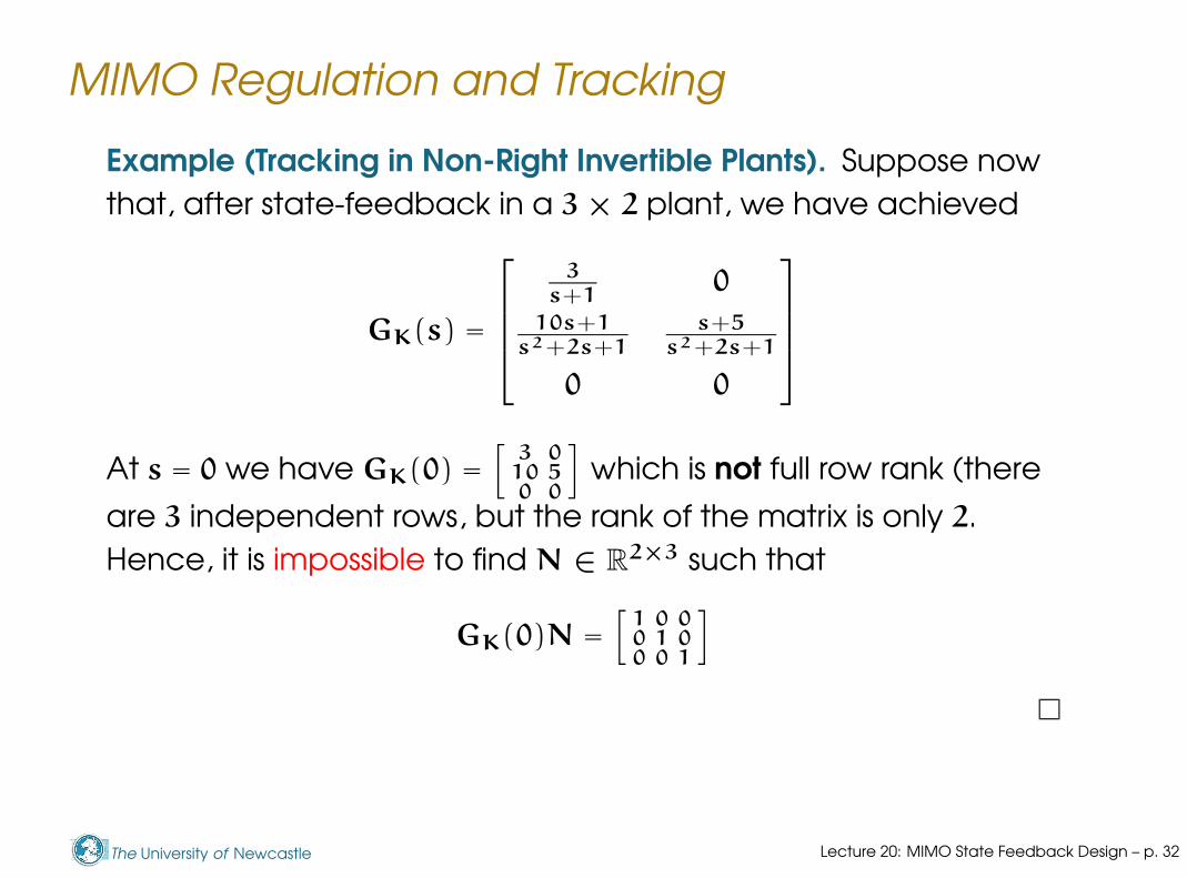
Example (Tracking in Non-Right Invertible Plants). Suppose now
that, after state-feedback in a 3 × 2 plant, we have achieved
GK(s) =
3s+1
0
10s+1s2+2s+1
s+5s2+2s+1
0 0
At s = 0 we have GK(0) =[
3 010 50 0
]
which is not full row rank (there
are 3 independent rows, but the rank of the matrix is only 2.
Hence, it is impossible to find N ∈ R2×3 such that
GK(0)N =[
1 0 00 1 00 0 1
]
Lecture 20: MIMO State Feedback Design – p. 32

The University of Newcastle
MIMO Regulation and Tracking
Tracking with Integral Action is subject to the same restrictions:
we can only achieve asymptotic tracking of a maximum of as
many outputs as control inputs are available.
Lecture 20: MIMO State Feedback Design – p. 33

The University of Newcastle
MIMO Regulation and Tracking
Tracking with Integral Action is subject to the same restrictions:
we can only achieve asymptotic tracking of a maximum of as
many outputs as control inputs are available.
The scheme and computation procedure is the same as in SISO
f
b
f f
b
fb bf ? - -
¾
¾6- ?- - - - - -
66- -
K
A
C
do(t)
y(t)B
di(t)
x(t) x(t)∫
−
u(t)r
−
∫ε(t)kz
z(t) −
Note that now the integral action is applied to each of the q
reference input channels.
−
−
−
∫
∫
∫∫+ ≡
r2
r3
y1 y2 y3
r1 ε1
ε2
ε3
Lecture 20: MIMO State Feedback Design – p. 33

The University of Newcastle
MIMO Regulation and Tracking
The procedure to compute K and kz for the state feedback
control with integral action is exactly as in the SISO case,
z(t) = r − y(t) = r − Cx(t)
u(t) =[
K kz
]
x(t)
z(t)
where Ka = [ K kz ] is computed to place the eigenvalues of the
augmented plant (Aa, Ba) at desired locations, where
Aa =
A 0n×q
−C 0q×q
, Ba =
B
0q×p
Lecture 20: MIMO State Feedback Design – p. 34

The University of Newcastle
Outline
A Note about Scaling
MIMO State Feedback Design
Cyclic Design
MIMO Regulation and Tracking
MIMO Observers
Lecture 20: MIMO State Feedback Design – p. 35

The University of Newcastle
MIMO Observers
A − LC
B
A
∫ x(t)CN
−
u(t)
∫L
B
Kx(t)
y(t)r x(t)
Observer
PlantDesign of MIMO obervers
extends directly from the
SISO case. To compute
the observer gain
L we can use “duality”
and the procedures
seen to compute
state feedback gains,
as the cyclic design.
Lecture 20: MIMO State Feedback Design – p. 36

The University of Newcastle
MIMO Observers
A − LC
B
A
∫ x(t)CN
−
u(t)
∫L
B
Kx(t)
y(t)r x(t)
Observer
PlantDesign of MIMO obervers
extends directly from the
SISO case. To compute
the observer gain
L we can use “duality”
and the procedures
seen to compute
state feedback gains,
as the cyclic design.
Alternatively, we can also use linear quadratic optimal design, to
obtain an optimal observer gain L. The observer obtained in this
way is usually called the Kalman filter.
Lecture 20: MIMO State Feedback Design – p. 36

The University of Newcastle
Reduced Order Observers
A technique that could be particularly useful in the MIMO
case is that of reduced order observer design.
Lecture 20: MIMO State Feedback Design – p. 37
The University of Newcastle
Reduced Order Observers
A technique that could be particularly useful in the MIMO
case is that of reduced order observer design.
One argument against state-feedback+observer controllers
is that they generally have high order:
since the observer includes a model of the plant, we would nor-
mally obtain a controller of at least of the same order of the open-
loop system.
Lecture 20: MIMO State Feedback Design – p. 37

The University of Newcastle
Reduced Order Observers
However, it is possible to reduce this order to some extent by
designing a reduced order observer.
The key observation is that
if the state equations are selected in such a way that the q system
outputs constitute the first q states, then in fact we only need to
estimate the remaining n − q states to apply state feedback.
KReduced Order
Observer
xy
xru
y
Lecture 20: MIMO State Feedback Design – p. 38

The University of Newcastle
Reduced Order Observers
Let the system equations be
y
xr
=
A11 A12
A21 A22
y
xr
+
B1
B2
u
where the first q states are the outputs of the system. Because
we measure the outputs, we could try and build an observer
only to estimate the remaining states xr.
xr = A22xr + A21y + B2u
yr , A12xr
Lecture 20: MIMO State Feedback Design – p. 39

The University of Newcastle
Reduced Order Observers
Let the system equations be
y
xr
=
A11 A12
A21 A22
y
xr
+
B1
B2
u
where the first q states are the outputs of the system. Because
we measure the outputs, we could try and build an observer
only to estimate the remaining states xr.
xr = A22xr + A21y + B2u
yr , A12xr = y − A11y − B1u︸ ︷︷ ︸measurable “output”
We can think of yr as a “virtual” output of a reduced order state
equation with state xr. We can compute everything in yr from
measurements; the only problem is that it appears we need y.
Lecture 20: MIMO State Feedback Design – p. 39

The University of Newcastle
Reduced Order Observers
Then the observer required to estimate the states xr can be
constructed as
˙xr = A22xr + A21y + B2u + Lr (yr − A12xr)
Lecture 20: MIMO State Feedback Design – p. 40

The University of Newcastle
Reduced Order Observers
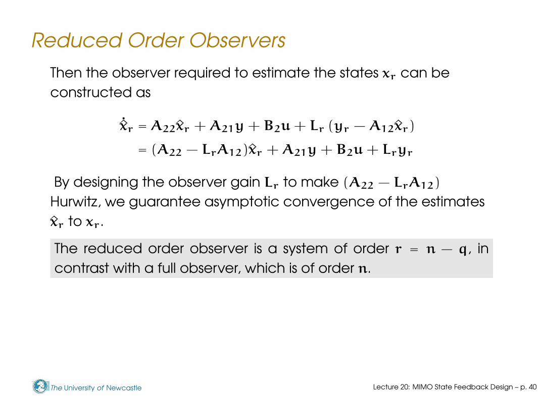
Then the observer required to estimate the states xr can be
constructed as
˙xr = A22xr + A21y + B2u + Lr (yr − A12xr)
= (A22 − LrA12)xr + A21y + B2u + Lryr
By designing the observer gain Lr to make (A22 − LrA12)
Hurwitz, we guarantee asymptotic convergence of the estimates
xr to xr.
Lecture 20: MIMO State Feedback Design – p. 40
The University of Newcastle
Reduced Order Observers
Then the observer required to estimate the states xr can be
constructed as
˙xr = A22xr + A21y + B2u + Lr (yr − A12xr)
= (A22 − LrA12)xr + A21y + B2u + Lryr
By designing the observer gain Lr to make (A22 − LrA12)
Hurwitz, we guarantee asymptotic convergence of the estimates
xr to xr.
The reduced order observer is a system of order r = n − q, in
contrast with a full observer, which is of order n.
Lecture 20: MIMO State Feedback Design – p. 40

The University of Newcastle
Reduced Order Observers
Then the observer required to estimate the states xr can be
constructed as
˙xr = A22xr + A21y + B2u + Lr (yr − A12xr)
= (A22 − LrA12)xr + A21y + B2u + Lryr
By designing the observer gain Lr to make (A22 − LrA12)
Hurwitz, we guarantee asymptotic convergence of the estimates
xr to xr.
The reduced order observer is a system of order r = n − q, in
contrast with a full observer, which is of order n.
The only “problem” with the reduced observer is that it appears
that we need to differentiate the output to compute yr!
yr = y − A11y − B1u
Lecture 20: MIMO State Feedback Design – p. 40

The University of Newcastle
Reduced Order Observers
We eliminate the need to differentiate the output by clever
implementation. We show how by block diagram algebra.
Lecture 20: MIMO State Feedback Design – p. 41

The University of Newcastle
Reduced Order Observers
We eliminate the need to differentiate the output by clever
implementation. We show how by block diagram algebra.
B
A
∫ x(t)C
u(t) y(t)
∫Lr
B2
xr(t)
A22 − LrA12
B1 A11
yr(t)
ddt
Reduced Order Observer
−
−
Lecture 20: MIMO State Feedback Design – p. 41
The University of Newcastle
Reduced Order Observers
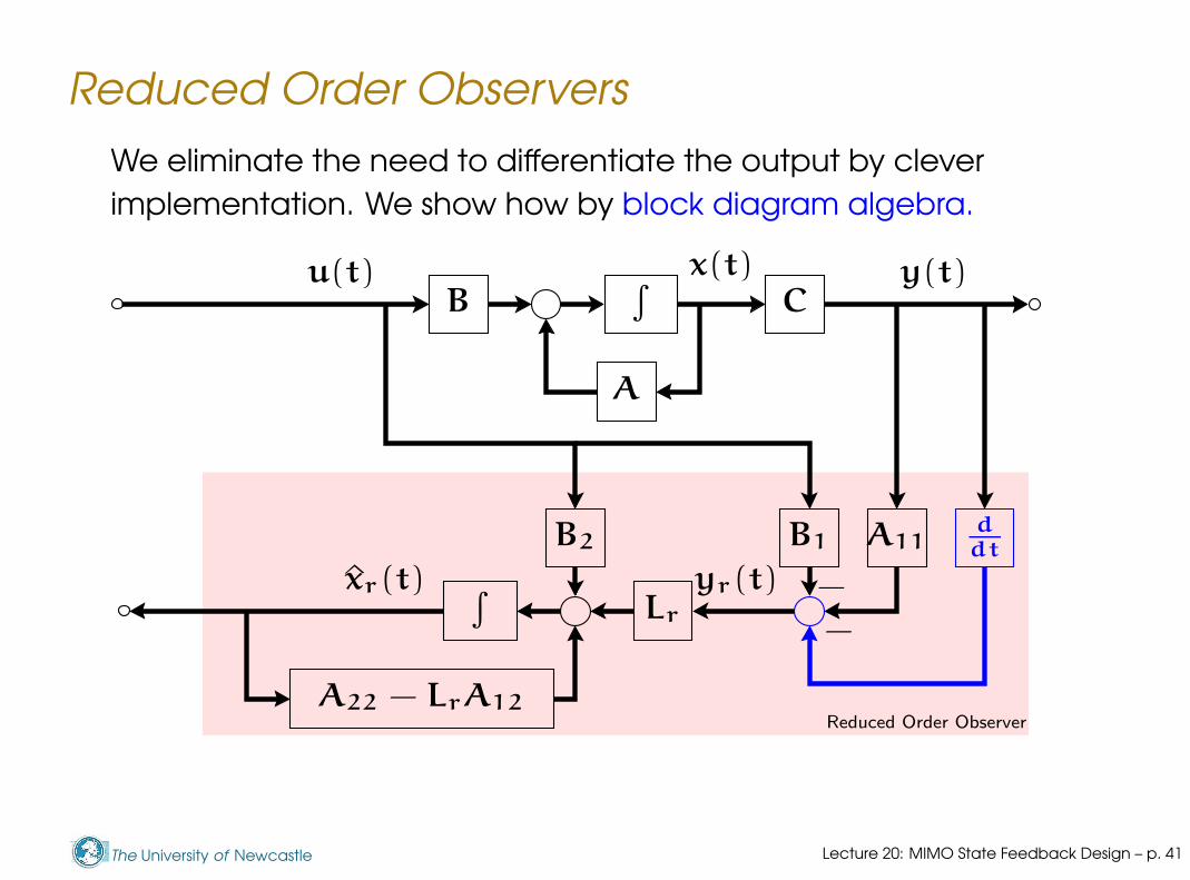
We eliminate the need to differentiate the output by clever
implementation. We show how by block diagram algebra.
B
A
∫ x(t)C
u(t) y(t)
∫Lr
B2
xr(t)
A22 − LrA12
B1 A11ddt
yr(t)
Reduced Order Observer
−
−
Lecture 20: MIMO State Feedback Design – p. 41

The University of Newcastle
Reduced Order Observers
We eliminate the need to differentiate the output by clever
implementation. We show how by block diagram algebra.
B
A
∫ x(t)C
u(t) y(t)
∫B2
xr(t)
A22 − LrA12
B1 A11ddt
Lr
Lr
Reduced Order Observer
− −
Lecture 20: MIMO State Feedback Design – p. 41

The University of Newcastle
Reduced Order Observers
We eliminate the need to differentiate the output by clever
implementation. We show how by block diagram algebra.
B
A
∫ x(t)C
u(t) y(t)
∫B2
A22 − LrA12
B1 A11
Lr
Lr
xr(t)
Reduced Order Observer
− −
Lecture 20: MIMO State Feedback Design – p. 41

The University of Newcastle
Summary
Scaling: The important points to remember:
Lecture 20: MIMO State Feedback Design – p. 42

The University of Newcastle
Summary
Scaling: The important points to remember:
State-space models are, in general, the most reliable
models for subsequent computations.
Lecture 20: MIMO State Feedback Design – p. 42

The University of Newcastle
Summary
Scaling: The important points to remember:
State-space models are, in general, the most reliable
models for subsequent computations.
Scaling model data can improve the accuracy of your
results.
Lecture 20: MIMO State Feedback Design – p. 42
The University of Newcastle
Summary
Scaling: The important points to remember:
State-space models are, in general, the most reliable
models for subsequent computations.
Scaling model data can improve the accuracy of your
results.
Numerical computing is a tricky business, and virtually all
computer tools can fail under certain conditions.
Lecture 20: MIMO State Feedback Design – p. 42

The University of Newcastle
Summary
Scaling: The important points to remember:
State-space models are, in general, the most reliable
models for subsequent computations.
Scaling model data can improve the accuracy of your
results.
Numerical computing is a tricky business, and virtually all
computer tools can fail under certain conditions.
MIMO state feedback and observer design extends directly
from SISO to MIMO systems. One significant difference in
state feedback for MIMO systems:
the state feedback gain K that place the closed-loop
eigenvalues of a MIMO system at desired locations is not
unique
Lecture 20: MIMO State Feedback Design – p. 42

The University of Newcastle
Summary
The “excess” of degrees of freedom in MIMO state feedback
design can be handled by
Lecture 20: MIMO State Feedback Design – p. 43
The University of Newcastle
Summary
The “excess” of degrees of freedom in MIMO state feedback
design can be handled by
Cyclic design, which reduces the problem to one of SIMO
— it requires the A matrix to be cyclic, or otherwise, an
extra state feedback to render it cyclic.
Lecture 20: MIMO State Feedback Design – p. 43

The University of Newcastle
Summary
The “excess” of degrees of freedom in MIMO state feedback
design can be handled by
Cyclic design, which reduces the problem to one of SIMO
— it requires the A matrix to be cyclic, or otherwise, an
extra state feedback to render it cyclic.
Optimal design, for example LQR, as we will see in coming
lectures.
MIMO regulation and tracking can be handled by the same
procedures used for SISO systems. Yet, one must be careful
that the tracking objectives be consistent with the feasible
tracking directions that the plant can reach.
Lecture 20: MIMO State Feedback Design – p. 43

The University of Newcastle
Summary
MIMO observers are designed in the same way as SISO
observers, and the state feedback design techniques can
be used via duality.
Lecture 20: MIMO State Feedback Design – p. 44
The University of Newcastle
Summary
MIMO observers are designed in the same way as SISO
observers, and the state feedback design techniques can
be used via duality.
Particularly interesting in the MIMO case is the possibility of
designing reduced order observers, which can significantly
reduce the order of the overall state feedback + observer
controller.
Lecture 20: MIMO State Feedback Design – p. 44