control structure integrated design - syracuse university · control structure integrated design...

Control Structure Integrated Design

Achille Messac

Kamal Malek

Corresponding Author

Achille Messac, Ph.D.

Distinguished Professor and Department Chair

Mechanical and Aerospace Engineering

Syracuse University, 263 Link Hall

Syracuse, New York 13244, USA

Email: [email protected]

Tel: (315) 443-2341

Fax: (315) 443-3099

https://messac.expressions.syr.edu/

Bibliographical Information Messac, A., and Malek, K. “Control Structure Integrated Design,” AIAA Journal, Vol. 30, No. 8,

Aug. 1992, pp. 2124-2131.

AIAA JOURNALVol. 30, No. 8, August 1992

Control-Structure Integrated Design

Achille Messac*Charles Stark Draper Laboratory, Inc., Cambridge, Massachusetts 02139

andKamal Malekt

Massachusetts Institute of Technology, Cambridge, Massachusetts 02139

This article presents an optimization-based approach to the integrated control and structural design ofdynamical systems. The framework of a general formulation is developed, which lends itself directly to thedesign of structural plants requiring control. This method can employ classical and modern control techniquesin the time or frequency domain. A performance norm that possesses full knowledge of the control and structuraldesign characteristics is developed. This article explicitly addresses the disturbance-rejection and command-following performance of the system, in addition to the vibration level and the control effort. The designmethodology is demonstrated by simultaneously performing the structural and control designs of a truss-likespacecraft undergoing a rotational maneuver.

Introduction

F UTURE military and commercial space systems will pre-sent increasingly stringent performance requirements. In

order to meet the challenge, prevailing design methods mustbe readdressed. Current design practices are characterized bya schism between the structural and the control design proc-esses. These two design phases are performed separately, fol-lowing two disparate paths, with little or no interaction. Thislack of interdisciplinary activity is not surprising however.Recent advances in computer technology are only beginningto have their full impact, and the development of effectivecontrol-structure integrated design (CSID) methods is far frombeing a solved problem. This publication takes only a step inthat direction.

The structural engineer generally designs a structural plantby relying on: 1) an overall knowledge of the mission objec-tives and constraints, 2) some limited understanding of thecontrol issues, and 3) experience and intuition. The typicalstructural design follows some iterative ad-hoc approach thatoften converges satisfactorily, or follows some form of struc-tural optimization. Unfortunately, the typical structural op-timization approach fails to recognize the properties of theas-yet-unknown control design.

The major limitation of structural optimization alone stemsfrom the objective function's inability to reflect total systemperformance. Typical objectives include: 1) minimum mass,2) uniform stress, 3) maximum fundamental frequency, and4) maximum damping. For instance, by indiscriminately in-creasing damping and stiffness in order to meet stringentpointing requirements, structural optimization may result inlarge system mass, and a correspondingly high control au-thority requirement.

With a structural design in near-final form and an in-depthknowledge of mission objectives and constraints, the controlengineers generally have at their disposal all the informationneeded to design a control system. Unfortunately, the controldesign phase has no appreciable impact on the structural design.

Received May 22, 1991; revision received Nov. 25,1991; acceptedfor publication Nov. 27, 1991. Copyright © 1991 by Charles StarkDraper Laboratory, Inc. Published by the American Institute ofAeronautics and Astronautics, Inc., with permission.

* Senior Member of the Technical Staff. Member AIAA.tDoctoral Candidate, Department of Mechanical Engineering.

As a result of this limited interdisciplinary interaction, thefinal system design is seldom optimal in any global sense. Thisis particularly true in the case of complex systems where ex-perience or intuition usually fails to produce optimal (or near-optimal) designs. In addition, although a control designercan easily determine the consequences of a control-designmodification on performance, the same is not true of thestructural designer. The latter's only recourse is experienceand intuition.

A new approach to designing dynamical systems with im-proved performance and robustness characteristics has beenunder development for the past decade. References 1-9 rep-resent but a small sample of the publications on the topic.This paper refers to this new approach as CSID. By recog-nizing the interrelated nature of the various system charac-teristics, and by explicitly representing the global mission ob-jective, an optimal balance between the structure and thecontrol system can be achieved. This design approach is char-acterized by full use of interdisciplinary knowledge through-out the design process. Significant required structural changescan be identified and effected early in the design process,when the cost consequences are less severe. Given typicalmass constraints and the trend toward more stringent per-formance requirements, CSID methods must be exploited forthe successful design of current and future space systems.7

The approach presented in this paper is highly computa-tional in nature. Closed-form analytical solutions for the ob-jective and constraints are employed in conjunction with non-linear numerical optimization techniques. A scalar measureof system performance is minimized, subject to certain prac-tical constraints. These constraints may include system sta-bility, system mass, structural member sizes, and robustness.The existence of a closed-form solution for any performancemeasure is critical to the computational feasibility of CSIDfor realistically large structures.

In the current approach, CSID nonlinear constrained op-timization is performed within a general framework. Modalreduction is employed to reduce computational effort. Thestructural design variables are chosen to effect mass, stiffness,and possibly damping redistribution. The control design var-iables are also general in nature. They can represent, amongother things, elements of feedback matrices, Q-parameteri-zation, or pole and zero location. LQR and LQG designsconstitute a natural subset of the possible applications.

There are strong advantages to the computational approachadvocated in this paper. Nonlinear programming methods

2124

MESSAC AND MALEK: CONTROL-STRUCTURE INTEGRATED DESIGN 2125

• % ^SPECS. I

r

RAINTSx\

PLANT

ds

CONTROL

dc

dsdcv i> z

CSID LOGIC

NEW ds dc

(SYSTEM DESIGN)

Fig. 1 CSID computational structure.

allow for explicit constraints on system characteristics. Timedomain specifications (settling time due to step commands,for example) and frequency domain requirements can be for-mulated as constraints. A purely analytical approach wouldnot offer such versatility.

Using this computational approach, CSID research can fo-cus on rendering existing control synthesis tools applicable toCSID.

As Fig. 1 shows, a top-level view of the CSID computationalstructure depicts a dynamical system with performance androbustness properties that are altered by a set of control andstructural design parameters. The constituent components ofthe CSID-logic block include numerically well-conditionedconstraint and objective functions. These are nonconvex func-tions of the design variables. The objective function is quad-ratically dependent on the error vector z(f). The plant-and-control design block comprises a state-space representationof the closed-loop system, which, in general, is a highly non-linear function of the structural and control design variablesds and dc. The inputs to the plant/control system are the ex-ogenous disturbance vector ud(f) and the reference signal vec-tor r(f), which have temporal or spectral properties that aredictated by system design specifications. The vector z(t) de-notes system response errors that the CSID-logic functionalblock attempts to minimize. These may include structuralvibration, control effort, or pointing error.

This paper is organized as follows. First, the full-order andreduced-order modeling of the structural system is developed.Second, a general framework for compensator modeling ispresented. Third, a new performance norm that addressesexplicitly the command-following and disturbance-rejectionproperties of the system is developed. Its favorable compu-tational properties were evidenced by successful CSID ap-plication. Fourth, the dynamics model of a truss-like space-craft is developed, and pertinent structural parameters areidentified for CSID application. Finally, the Results and Dis-cussion section shows the power of CSID to identify improvedsystem designs.The advantage of using CSID, rather thancontrol optimization alone, is quantified.

Plant Dynamics ModelingPhysical Coordinate Representation

The plant considered in this paper consists of a structuralsystem with governing dynamics equations that are assumedto obey the well-known set of coupled second-order differ-ential equations. Applying finite element methods, the equa-tions are written in the form

M(ds)q + D(ds)q + K(ds)q = Bqcuc 4- Bqdud (1)

where M, D, and K respectively denote the mass, damping,and stiffness matrices that depend on a set of structural designvariables ds. These variables are capable of altering the geo-

metrical properties of the structure and its mass, damping,and stiffness distributions. The vector q denotes the physicalcoordinates of the structure; uc and ud are the control anddisturbance forces and torques, respectively, while Bqc andBqd denote the corresponding influence coefficient matrices.The above segregation of controls and disturbances will laterallow addressing the command-following and disturbance-re-jection problems (Eqs. (42-43)). The specific time history ofud is in general unknown; only some of its time or frequencydomain characteristics are assumed. In this article, the vectorud is assumed to be composed of impulses of known intensities.

For analytical convenience, we construct a standard statespace representation of Eq. (1), and append observation anderror equations, thus:

xq = Aqxq + Bxcuc + Bxdud

zp = Czqxq + Dquc

y = cyqxq

(2)

(3)

(4)

The vectors y and zp are, respectively, the observation anderror vectors. The state vector is

-MUJ (5)

The plant error vector does not include ud because ud cannotbe minimized. The dynamics matrix takes the form

= [ 0\_-M~l1K -M~1D

The influence coefficient matrices are

(6)

Bvf = Bxd~ ~IB JEquations (2-7) govern the plant dynamics. These equa-

tions are generally adequate for the analysis of low-orderstructural systems. In the case of large structures, however,model order reduction is required.

Modal Coordinate RepresentationWith high-order structural applications in mind, plant model

reduction is performed via model decomposition. A lineartransformation is performed, based on a subset of the modalspace basis. The transformation is

q = <E>i7 (8)

Normalization and other required definitions take the form

A, = A,S, (10)

where 8^ is the Dirac delta function, and

D^ = D^ds), A == A(d5), O = ^(ds) (11)

The quantities <I> and A respectively denote the truncatedmodal and eigenvalue matrices of the system. The matrix D^denotes modal damping, and takes a diagonal form in thecase of low viscous damping.

The reduced-order form of the state equation is again writ-ten in its generic form as

(12)

2126 MESSAC AND MALEK: CONTROL-STRUCTURE INTEGRATED DESIGN

where the modal state vector is

The state equation dynamical matrix reads

-ij

(13)

(14)

(15)

(16)

The influence coefficient matrices are

The output and error coefficient matrices are

Czr, = = D

(18)

(19)

Compensator RepresentationThe compensator employed in this paper assumes the ge-

neric form of a matrix transfer function. Specifically, for amultiple-input-multiple-output (MIMO) system, the compen-sator dynamics take the form

uc(s) = GC( (20)

r ni[8R (

w3n ck=\

s +

s +

n2<*k) n o«4dk) n o

fc = l

?2 + fc*S

?2 + eks

+ c

+ /4,)

where uc and zc respectively denote the generalized controland the error vectors, and Gc(s) denotes the compensatortransfer function matrix. The constituent elements of Gc(s)are expressed as

(21)

where the quantities g, 0fc, bk, . . . , fk are parameters thatcharacterize the properties of the controller, and the indicesi and/ denote the (i/)th element of the transfer matrix Gc(s).These parameters collectively constitute the set of controldesign variables.

By defining

vtj = fe, fll, . . . , flnl, f r l 9 . . . , bn2, cl9..., cn2}, (22)

and

w = {dl7 . . . , dn3, el9 . . . , cB4,/i» - - • ,/nJ (23)

the control design variable vector becomes

dc = {vn, . . . , v1/? . . . , v^, . . . , vkh w} (24)

As can be seen, the number of design variables can growrapidly for MIMO systems. Fortunately, in practice the matrixcompensator transfer function is not necessarily fully popu-lated, nor comprised of elements of high order.

Initial values for the control variables can be obtained throughconventional means such as using Matlab with the initial modelof the plant. Because the CSID method in this paper is per-

formed in state space, the state equation representation ofthe compensator is obtained in the standard form

xc(t) = Acxc(t)

uc(t) = Ccxc(f)

Bczc(t)

Dczc(f)

(25)

(26)

where xc denotes the controller state vector and the matricestake on standard definitions. With the development of bothplant and compensator, it is possible to form the closed-looprepresentation of the system.

Closed-Loop RepresentationThe state equations of the closed-loop system are obtained

by combining the structure (Eqs. (12-14)) and the controller(Eqs. (25) and (26)), and by defining the error variable as

zc(f) = r(f) - y(t) (27)

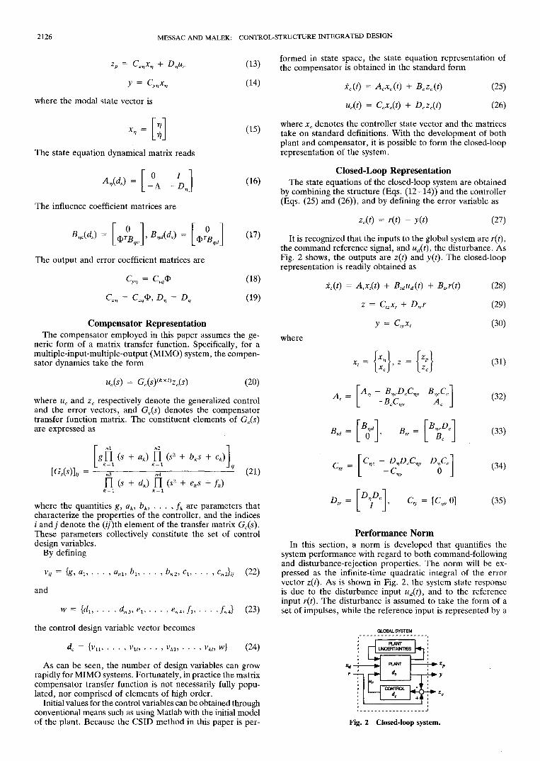
It is recognized that the inputs to the global system are r(f),the command reference signal, and ud(t), the disturbance. AsFig. 2 shows, the outputs are z(f) and y(f). The closed-looprepresentation is readily obtained as

xt(f) = Atxt(t) + Btdud(t)

z = Ctzxt + Dtrr

Btrr(f)

where

B _a"~ Bc

=

"

D" = [D*IDe]' Cly =

(28)

(29)

(30)

(31)

(32)

(33)

(34)

(35)

Performance NormIn this section, a norm is developed that quantifies the

system performance with regard to both command-followingand disturbance-rejection properties. The norm will be ex-pressed as the infinite-time quadratic integral of the errorvector z(t). As is shown in Fig. 2, the system state responseis due to the disturbance input ud(t), and to the referenceinput r(i). The disturbance is assumed to take the form of aset of impulses, while the reference input is represented by a

GLOBAL SYSTEM

Fig. 2 Closed-loop system.


prescribed set of step commands. Therefore, the system statevector time history is expressed as

xt(f) = eA^-^xt(r) + J e

[Btdud(cr) + Btrr(a)]do- (36)

To obtain an expression for z(f) when T and xt(ty are setto zero, one first writes the sum of the separate contributionsof reference and disturbance input as

z(f) = zd(f) + zr(i)

in which case

*<•« =

(t) = \Jo

Specifically, let

; t<Q

which leads to

z,(t) = [Dlr - C!zArlB,,]

(37)

(38)

(39)

(40)

(41)

With the appropriate framework for the controller (sufficientnumber of zeros, etc.), the steady-state error can be made tovanish identically, leading to

Similarly

z,(i) = C^'A^BJ , t > 0

zd(i) = C^'BJlt ,t>0

(42)

(43)

where ud denotes the impulse intensity vector. The perform-ance norm is now expressed as the infinite-time quadraticintegral of the error vector z(t) as (See Eq. (37))

(44)

(45)

J(ds, dc) = (zr + zd)TQ(zr

or, in expanded form

J(ds, dc) = Jrr + 2Jrd + Jdd

where j- = \ r zwQz-w\

(47)

(48)

and where the matrix Q is a symmetric positive semidefiniteweighting matrix. To evaluate the above integrals, it is con-venient to first perform the modal decomposition

which leads to the new expressions

zr(t) = CeAtA~lBrr7

zd(f) = Ce^Bdud,

where

C = CtzX, Br = YBtr,

After some manipulation, one obtains

Jrr(ds, dc) = \rTBtSr

JrM, dc) =

Jdd(ds, dc) =

t > 0

t > 0

Bd = YBt

(50)

(51)

(52)

(53)

(54)

(55)

where

(£,)«, = -

(Srd)i/ = -

(Gk,. + A,.)Ay

(6).,A,(A, + A,)

e = crgc

(57)

(58)

(59)

The above performance norm offers an important tool indesigning, analyzing, and evaluating high-performance sys-tems. It is possible to trade between the disturbance-rejectionand the command-following properties of the system by ap-propriately selecting the vectors r and u. In addition, therelative intensities of structural vibrations and generalizedcontrol forces are regulated directly by appropriately struc-turing the plant error (Eqs. (2-4)) and the matrix 2, Eq.(44). To see this, simply write Eq. (3) in the form

" - tl -(60)

where zpu(t) denotes the control, and zpz(f) denotes the vi-bration level. Therefore, the plant error vector can segregatecontrol from vibration. Moreover, it is helpful to write theerror vector as (see Eqs. (31 and 60))

(= f\ (61)

and the weighting matrix, in block diagonal form, as (see Eqs.(44 and 37)). Reference 9 treat the situation where closed-loop zero eigenvalues exist.

Q =

QPU

0

0

QPZ

0

0

Qc

(62)

At = XAY, XY - /, Ktj = X&j (49)

Mathematical Problem StatementThe system dynamics equations and the performance norm

are now used to formulate the CSID nonlinear programming


problem formally as

min J(ds,

subject to

a, s gi(ds, dc) < ft

(63)

(64)

Equation (64) denotes constraint conditions that directlycontrol system design specifications. These constraints in-clude: 1) nominal or robust stability, 2) system mass, 3) struc-tural member sizes, 4) geometry, and 5) frequency and/ortime domain behavior.

It is recalled that the performance measure is a highly non-linear integral function of the system dynamics equations and,in general, is not a convex function of the control and struc-tural design variables. The numerical conditioning propertiesof both the objective and constraint functions are the key toa successful solution, especially in the case of high-order struc-tures. The performance norm developed in this paper doesdisplay highly favorable numerical conditioning properties,and its evaluation involves numerical procedures for whichrobust digital algorithms exist.

The commercial code GRG2 (Generalized Reduced Gra-dient 2)11 was employed as the optimization module of theCSID simulation. It was found to be numerically robust. Therequired gradients were evaluated via finite-difference meth-ods. As with all nonconvex optimization problems, the al-gorithm might converge to a local minimum. The typical safe-guards are therefore in order. These include: 1) restarting theproblem with a different initial condition, 2) rescaling theproblem periodically during optimization, and 3) starting froma reasonable initial condition, and so forth. Unfortunately,even with those precautions, convergence to the global min-imum is not guaranteed. Detailed knowledge of the nonlinearoptimization method, together with deep understanding ofthe problem, are the real saviors.

Spacecraft ExampleProblem Statement

A spacecraft is used as an example to demonstrate the CSIDapproach proposed in this paper (Fig. 3a). This structure con-sists of a central rigid hub to which two appendages are sym-metrically attached. Each truss-like appendage carries a lumpedmass at its tip. Under normal operation, this spacecraft under-goes planar rotational maneuvers about the inertially fixedaxis k. The penalty on the control effort, the tip vibration,and the command-following error are (see Eq. (62))

pu, QP2, QJ = (0, £ 1} (65)

It is noted that a nonzero value of the control penalty and amore complex compensator structure are effective means offurther improving system response (shorter settling-time, etc.).

The geometrical symmetry, in addition to the purely ro-tational motion of the spacecraft, permits the assumption ofan antisymmetric deformation field. Figure 3b depicts thespacecraft kinematics. The body frame is embedded at thecenter of the rigid hub and is denoted by the dextral triad z,7, k. The vector ut denotes the translational deformation ofnode /, and /,- denotes its longitudinal coordinate. The vectorr represents the hub radius, and / represents the appendagelength. The equations of motion are obtained by applyingthe finite element method (FEM) in conjunction with theNewton-Euler equations.

The two trusses are modeled as a set of interconnectedbeam elements, each representing a bay. The generic space-craft described is assumed to comprise 50 bays (25 per ap-pendage). All beam elements have the same length le, and

Fig. 3a Example spacecraft.

Fig. 3b Spacecraft kinematics.

the same width w. The lateral dimension of each elementvaries as the structure is optimized. The spacecraft inertialcharacteristics are modeled using a lumped mass formulation,where the nodal masses are assumed to be purely translational.

Dynamics EquationsThe equation of motion development involves four steps.

Step 1: ith Mass Translational EquationBy applying Newton's law, the equation that governs the

motion of the ith nodal mass along the 7 axis can be writtenas

where mt is the nodal mass, 0 is the inertial rotation of thehub, fintti denotes the internal elastic forces, and ft accountsfor externally applied forces at node i. To obtain an explicitexpression for the internal forces, the global stiffness matrixof the cantilevered truss is formed, followed by static con-densation of the rotational degrees of freedom. This resultsin a stiffness matrix Ktt, which relates the internal forces tothe deformation coordinates as

(67)

The subscript tt denotes that only the translational degrees-of-freedom are retained in the static condensation.

Equations (66) and (67) are cast in matrix form as

where

and

Mttu + SO + Kttu = f

Mtt = diag(m1?

ST =

(68)

(69)

(70)

Step 2: Spacecraft Rotational EquationThe rotational equation is obtained by satisfying rotational

inertial equilibrium of the spacecraft. Doing so leads to

1,0 + 2STu = rh 2 2 (71)


Table 1 Spacecraft properties

Spacecraft properties ValuesTip massHub inertia 70Appendage lengthNumber of elements per appendageHub radiusInitial beam widthBeam depth (constant)Beam volumetric densityBeam modulus EDamping ratio

2kg4000 kg/m2

20m251.0m0.05m0.01 m1000 kg/m3

1011 N/m2

0.5%

where

- 4 2 2 (72)

is the system total inertia, 7hub is the hub rotational inertia,and thub denotes the external torque applied to the hub.

Step 3: Global EquationsThe global set of equations that governs the system dynam-

ics in physical coordinates takes the form

Mq K — P F*^q ~ rqrq

where

qT = {0, ul9 . . . , un_l}

£]• '-[Si]0 1

0

Further, let (see Eq. (1))

~rj _

/--I

= Bqcuc + Bqdud

= PqEc

where Er and EH are row selection matrices.

(73)

(74)

(75)

(76)

(77)

(78)

(79)

Step 4: State EquationsThe full set of state equations is obtained in accordance

with the notation of the dynamics modeling section. The sca-lars df denote the set of structural design variables.

System CharacteristicsTwo actuation cases are considered: torque at the hub,

and antisymmetric forces applied along the appendages. Onlyhub angular position is fed back to the controller. Tip dis-placement is sensed and penalized via the objective function(see Eq. (65)). A 12th-order structural model was retained,and a third-order compensator with three zeros was em-ployed. A 15th-order system model with 50 structural designvariables was deemed adequate to demonstrate the currentmethodology.

Table 1 shows the numerical values used.

Results and DiscussionResults obtained using the above spacecraft model dem-

onstrate the effectiveness and flexibility of the proposed CSID

approach. These results show that the previously derived normis effective and numerically well conditioned for performingcontrol and structural optimization. It is also shown that theCSID methodology results in much improved response com-pared to control optimization alone. These improvements arenot easily identifiable via conventional design methods.

The proposed approach is computationally robust, as allthe results presented rely on a low-order compensator (third-order) and, in some cases, the sensor and actuators are notcolocated. In addition, optimized designs were obtained start-ing with rather poor compensators. Via numerous numericalsimulations, it is observed that the lower the compensatororder, the worse the performance, but also the worse thenumerical conditioning of the problem as a whole.

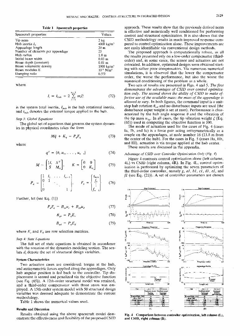
Two sets of results are presented in Figs. 4 and 5. The firstdemonstrates the advantages of CSID over control optimiza-tion only. The second shows the ability of CSID to make ef-fective use of the available mass: the mass of the appendage isallowed to vary. In both figures, the command input is a unit-step hub rotation 0ref and no disturbance inputs are used (thedisturbance input weight is set at zero). Performance is char-acterized by the hub angle response 0 and the vibration ofthe tip mass wtip. In all cases, the tip vibration weight £ (Eq.(65)) used in computing the objective function is 100.

The mode of actuation used for the cases of Fig. 4 (casesla, Ib, and Ic) is a force pair acting antisymmetrically as acouple on the appendages, at node number 16 (13.8 m fromthe center of the hub). For the cases in Fig. 5 (cases Ha, lib,and III), actuation is via torque applied at the hub center.

These results are discussed in the appendix.

Advantage of CSID over Controller Optimization Only (Fig. 4]Figure 4 contrasts control optimization alone (left column,

4L) vs CSID (right column, 4R). In Fig. 4L, control optim-ization is performed by optimizing the seven parameters ofthe third-order controller, namely g, al, bl, cl, dl, el, andfl (see Eq. (21)). A set of controller parameters are chosen

11.0

-20040

I 0

Time (s)

Frequency Response

Frequency (rad/s)

Appendage Profile

M appendage (kg)Mtip (kg)

I total (Kg.m2)f l (Hz>f 2 ( H z )

Uniform struct.Baselinecontroller

5.12.0

73460.0860.511

Optimizedcontroller5.12.0

73460.0860.511

M appendage (kg;

zfah(R)

Fig. 4 Comparison between controller optimization, left column (L),and CSID, right column (R).


Step Command

Mtip dm)I tori nC?.mZ>

— (HB —

Uniform struct.SSSGr

108853

1,0«

CSIDConstant Mass

107195

0.2140.937

Maroendaae (kgMtip (kg)

I total (Kj?.m2)f l <mf2(Hz)

Uniform struct.c»!r

10.02.0

88530.2191.063

CSIDFree Mass

922.0

71940.2150.930

(L) (R)

Fig. 5 CSID: Comparison of constant-mass, left column (L), andfree-mass, right column (R) cases.

as a starting point for the optimization. The response of theclosed-loop system with that starting or baseline controller(case la) is shown by the dashed lines. The response of theclosed-loop system using the optimized controller (see Ib) isshown by the solid lines.

The first two plots show the response to a unit step com-mand in the reference hub angle. The starting controller re-sults in poor response, as no significant effort was expendedon its selection. The hub response exhibits an overshoot ofabout 80%. The tip displacement is quite large and poorlydamped. The optimized controller reduces the displacementby approximately an order of magnitude. However, that im-provement is achieved at the expense of the hub response,which becomes very sluggish. That performance reflects thechoice of weights on control, hub position error, and tip dis-placement used in computing the objective function. It alsoreflects the low order of the controller.

The next two plots show the hub angle frequency responseand the tip displacement frequency response, respectively, toa desired hub angle input. The frequency responses exhibitthe same behavior already seen above. With the baselinecontroller, the hub response has an underdamped peak atapproximately 0.7 rad/s, reflecting the overshoot in the stepresponse. The optimized controller eliminates that peak, butalso reduces the bandwidth of the system (the response visiblydrops below 0 dB above 0.02 rad/s, and it stays below thatof the baseline controller from that frequency on). All res-onant peaks are reduced. The tip frequency response alsomirrors the step response. Compared to the baseline system,the low-frequency (0.7 rad/s) peak is eliminated, which ex-plains the absence of the low-frequency component in thestep response. The amplitude of the peak at 0.5 rad/s, whichcorresponds to the high-frequency component of the step re-sponse, is reduced significantly: its H^ norm (Ref. 10) is re-duced by about 20 dB. The tip response remains below thatof the baseline system for all frequencies above 0.02 rad/s.

The last plot in that column shows the geometric profile ofthe appendages for the optimized case; that profile is uniform,as structural optimization was not allowed in this case.

The table at the bottom of the column gives some of thespacecraft parameters. The controller parameters for the var-ious cases are given in the appendix.

Figure 4R contrasts the case of the optimized controllerdiscussed above (case Ib), now represented by the dashedlines, to the case where structure and controller parametersare optimized concurrently using the CSID methodology (caseIc), given by the solid lines. The CSID case exhibits improvedhub and tip step response. The hub response rise time isreduced from approximately 115 s to less than 35 s, with about20% overshoot, however a consequence of the choice ofweights, and of the low-order compensator used. Tip dis-placement response is reduced significantly.

These improvements can also be seen in the frequency re-sponse plots. Hub bandwidth is extended from about 0.02rad/s to about 0.1 rad/s with a slightly underdamped peak.Tip response amplitude is significantly reduced (by up to 50dB) at all frequencies up to about 1.5 rad/s.

These improvements are the result of the reshaped appen-dages, the profile of which is shown in the fifth plot. In termsof the objective function J (see table at bottom of each col-umn), CSID provides a reduction by a factor of eight com-pared to optimizing the controller parameters only.

CSID and Mass Constraint (Fig. 5)Figure 5 shows the ability of CSID to make effective use

of the available mass. The appendage mass is first constrainedto its original values (Fig. 5L), then allowed to vary (Fig. 5R).When the appendage mass is constrained, the optimizationprocess places the excess-mass where it has the least effect(near the hub). When the appendage mass is left free, CSIDremoves the excess-mass, resulting in reduction of systemmass. Hub torque actuation is used in this case.

The optimized CSID cases (cases lib and III) are given bythe solid lines in Figs. 5L and 5R. A baseline case (case Ha),which corresponds to a uniform nonoptimized structure, alongwith a third-order compensator, is given by the dashed linesfor reference. Again, no serious effort was expended on tun-ing the baseline compensator. The only difference betweenthe two CSID cases is the total appendage mass. In case lib,the mass of the appendage is constrained to remain constantat 10 Kg. In case III (Fig. 5R), that constraint is removed.

It is interesting to note how the appendage mass is distrib-uted in these two cases. Because the actuation torque is ap-plied at the hub and no force acts on the appendage itself,the profile of the latter tapers uniformly toward the tip. Inthe first case (case lib), a significant amount of mass is movedto the first element, next to the hub, in order to reduce thetotal rotational inertia of the system. This reflects the weightschosen for hub angle error and tip vibration (increasing thelatter to 1000 causes that excess mass to get redistributed alongthe beam).

The hub and tip step responses do not exhibit significantdifferences between the two cases of interest (cases lib andIII). Similarly, the frequency responses do not differ much.The message here is: "The same level of performance couldbe obtained with a lighter structure." CSID was an effectiveavenue to finding this lighter structure. The appendage massis reduced by about 8% in this process.

ConclusionA new optimization-based approach to the integrated con-

trol and structural design of large space structures has beenpresented, and its effectiveness successfully demonstrated inthe design of a maneuvering truss-like spacecraft. The com-putational framework of the formulation offers great versa-tility in that it can accommodate most state-of-the-art controltechniques. A performance norm is developed, which is nu-merically well behaved, and particularly well suited for CSIDapplication. Results show that the CSID approach presentedin this paper provides a methodical means for obtaining bothimproved control and structural designs.


Table Al Controller parameters for Fig. 5

Parameter

g

fi

Case laUniformstructurebaseline

controller£ = 100

0.1500E + 10.5400E - 1

-0.8000E - 10.3900E + 10.1400E + 00.4500E + 10.2900E + 1

Case IbUniformstructureoptimizedcontroller£ = 100

0.1706E + 00.9541E - 6

-0.3110E + 00.3896E + 10.4162E - 10.4502E + 10.2903E + 1

Table A2 Controller parameters for

Parameter

g

fi

Case HaUniform structurebaseline controller

£ = 1000.1500E + 20.1500E + 00.2000E + 10.4000E + 10.1600E + 10.1000E + 10.3000E + 1

Case lib

Case IcOptimizedstructure

and controller(CSID)£= 100

0.1837E + 10.9945E - 6

-0.7979E - 10.3902E + 10.1081E + 00.4499E + 10.2898E + 1

Fig. 6

Case IIICSID CSID

constant mass free mass£ = 100 £ = 100

0.1226E +0.9579E -

-0.6129E -0.4307E +0.6228E -0.4303E +0.2784E +

2 0.1229E + 26 0.9577E - 61 0.5603E + 01 0.4308E + 11 0.6327E - 11 0.4763E + 11 0.2784E + 1

AppendixThe controller parameters, used in each of the cases dis-

cussed in the Results and Discussion section, and shown inFigs. 4 and 5, are given in the Tables Al and A2. The pa-rameters correspond to those defined in Eq. (21).

AcknowledgmentsThis work was sponsored by the Charles Stark Draper Lab-

oratory Inc. under IR&D Project 301. The authors express

their gratitude to the reviewers and to the editor for theirvaluable remarks and suggestions.

ReferencesMessac, A., and Turner, J. D., "Dual Structural Control Optim-

ization of Large Space Structures," A1AA Dynamics Specialists Con-ference, Paper 84-1042-p, Palm Springs, CA, May 17-18, 1984.

2Messac, A., Turner, J. D., and Soosaar, K., "An Integrated Con-trol and Minimum-Mass Structural Optimization Algorithm for LargeSpace Structures," NASA JPL, Workshop on Identification and Con-trol of Flexible Space Structures, JPL 85-29, San Diego, CA, July 4-6, 1984.

3Milman, M., Salama, M., Schad, R., Bruno, R., and Gibson,J. S., Integrated Control-Structures Design: A Multiobjective Ap-proach, JPL D6767, Jet Propulsion Laboratory, Pasadena, CA, Jan.1990.

4Onoda, J., and Haftka, R. T., "An Approach to Structure/ControlSimultaneous Optimization for Large Flexible Spacecraft," AIAAJournal, Vol. 25, No. 8, 1987, pp. 1133-1138.

5Belvin, W. K., and Park, K. C., "Structural Tailoring and Feed-back Control Synthesis: An Interdisciplinary Approach," Journal ofGuidance, Control, and Dynamics, Vol. 13, No. 3, 1990, pp. 424-429.

6Rao, S. S., Venkaya, V. B., and Khot, N. S., "Game TheoryApproach for the Integrated Design of Structures and Controls,"AIAA Journal, Vol. 26, No. 4, 1988, pp. 463-469.

7Newsom, J. R., Layman, W. E., Waites H. B., and Hayduk,R. J., "The NASA Controls-Structures Interaction Technology Pro-gram," Forty-First Congress of the International Astronautical Fed-eration, Dresden, Germany, Oct. 6-12, 1990.

8Kirk, C. L., and Junkins, J. L., "Dynamics of Flexible Structuresin Space," Proceedings of the First International Conference at Cran-field United Kingdom, 15-18 May 1990, Springer-Verlag, New York.

9Messac, A., Caswell, R., and Henderson, T., "CSID ControlStructure Integrated Design: Centralized vs Decentralized Control,"AIAA 1st Aerospace Design Conference, The Impact of Multidis-ciplinary Design Optimization, Irvine, CA, February 3-6, 1992.

10Maciejowski, J. M., Multivariable Feedback Design, Addison-Wesley, Reading, MA, 1989, p. 15.

nLasdon, L. S., and Waren, E. D., GRG2 User's Manual, De-partment of General Business, School of Business Administration,Univ. of Texas, Austin, TX.

control structure integrated design - syracuse university · control structure integrated design...

Documents