control of pde–ode cascades with neumann interconnectionsflyingv.ucsd.edu/papers/pdf/128.pdf ·...

Journal of the Franklin Institute 347 (2010) 284–314

Control of PDE–ODE cascades withNeumann interconnections

Gian Antonio Sustoa,b, Miroslav Krstica,!

aDepartment of Mechanical and Aerospace Engineering, University of California at San Diego, La Jolla,CA 92093-0411, USA

bDepartment of Information Engineering, University of Padova, 35131 Padova ITA, Italy

Received 23 June 2009; received in revised form 16 September 2009; accepted 17 September 2009

Abstract

We extend several recent results on full-state feedback stabilization and state estimation ofPDE–ODE cascades, where the PDEs are either of heat type or of wave type, from the previouslyconsidered cases where the interconnections are of Dirichlet type, to interconnections of Neumanntype. The Neumann type interconnections constrain the PDE state to be subject to a Dirichletboundary condition at the PDE–ODE interface, and employ the boundary value of the first spatialderivative of the PDE state to be the input to the ODE. In addition to considering heat-ODE andwave-ODE cascades, we also consider a cascade of a diffusion–convection PDE with an ODE, wherethe convection direction is ‘‘away’’ from the ODE. We refer to this case as a PDE–ODE cascade with‘‘counter-convection.’’ This case is not only interesting because the PDE subsystem is unstable, butbecause the control signal is subject to competing effects of diffusion, which is in both directions inthe one-dimensional domain, and counter-convection, which is in the direction that is opposite fromthe propagation direction of the standard delay (transport PDE) process. We rely on the diffusionprocess to propagate the control signal through the PDE towards the ODE, to stabilize the ODE.& 2009 The Franklin Institute. Published by Elsevier Ltd. All rights reserved.

Keywords: Delay systems; Distributed parameter systems; Backstepping; Stability; Cascade systems

ARTICLE IN PRESS

www.elsevier.com/locate/jfranklin

0016-0032/$32.00 & 2009 The Franklin Institute. Published by Elsevier Ltd. All rights reserved.doi:10.1016/j.jfranklin.2009.09.005

!Corresponding author.E-mail address: [email protected] (M. Krstic).

www.elsevier.com/locate/jfranklin

dx.doi.org/10.1016/j.jfranklin.2009.09.005

mailto:[email protected]

1. Introduction

We consider cascade connections of PDEs, whose states are denoted as u!x; t", wheretZ0 is time and x 2 #0;D$ is the spatial domain, and ODEs whose states are denoted asX !t" 2 Rn. ODE systems of the form

_X !t" % AX !t" & Bu!0; t"; !1"

with PDE systems of the form

ut % ux; !2"

which is a delay/transport PDE, were considered in [3,12,13] and more recently in [9,10].The PDE system

ut % uxx !3"

is a heat PDE and it was considered in [7]. Finally, the PDE system

utt % uxx !4"

is a wave PDE and it was considered in [8]. In each of the three PDE models, (2)–(4), thecontrol enters through a boundary condition,

u!D; t" % U!t"; !5"

namely, at the end x % D of the domain #0;D$, which is opposite from the end x % 0 wherethe PDE and ODE connect.

The PDE state enters the ODE (1) through the variable u!0; t", which we refer to as aDirichlet interconnection. Unlike this interconnection, which was studied in [7,8,10], the‘‘Neumann interconnection,’’

_X !t" % AX !t" & Bux!0; t"; !6"

has not been studied yet. In this paper we study heat and wave PDEs connected in cascadewith an ODE, via a Neumann interconnection. As in [7,8,10], the only assumption weimpose is that !A;B" is a controllable pair.

We provide infinite-dimensional full-state feedback laws with explicit gain kernels thatcompensate the PDE dynamics and achieve stabilization of the PDE–ODE system.The key tool in this work is the continuum version of backstepping method[1,2,4,5,11,16,18] which employs infinite-dimensional transformations for the design ofthe controller and Lyapunov functions for the stability proof.

Next, we briefly review the existing results with Dirichlet interconnections. ODE systemswith input delay were considered in [10]. For the system

_X !t" % AX !t" & BU!t'D"; !7"

where D is an arbitrarily long delay, the backstepping approach yields the controller

U!t" % K eADX !t" &Z t

t'D

eA!t's"BU!s" ds! "

: !8"

This infinite-dimensional feedback law turns out to be identical to the classical predictorand finite-spectrum assignment feedback laws [3,12,13] and it represents a ‘‘delay-compensated’’ version of the nominal controller

U!t" % KX !t"; !9"

ARTICLE IN PRESSG. Antonio Susto, M. Krstic / Journal of the Franklin Institute 347 (2010) 284–314 285

where the bracketed term in (8) is a D-seconds ahead predictor of X !t", starting fromX !t" as an initial condition, and driven by the input history over the D-second window.While recovering the classical designs [3,12,13], the backstepping approach [10]also provides the first construction of a Lyapunov function for the predictor feed-back. The Lyapunov function allows various robustness studies, which were conductedin [6].In [7] a PDE–ODE cascade structure is studied, but for diffusive dynamics at the input

of the ODE, namely, for the heat PDE in cascade with an ODE, with a Dirichletinterconnection:

_X !t" % AX !t" & Bu!0; t"; !10"

ut!x; t" % uxx!x; t"; !11"

ux!0; t" % 0; !12"

u!D; t" % U!t": !13"

In this case, the backstepping approach yields the controller

U!t" % K#I 0$ e

!0I

A0

"D I

0

! "X !t" &

Z D

0

Z D'y

0e

!0I

A0

"sdx

0

B@

1

CAB

0

! "u!y" dy

8><

>:

9>=

>;: !14"

Finally, in [8], a wave PDE in cascade with an ODE, namely, the system

_X !t" % AX !t" & Bu!0; t"; !15"

utt!x; t" % uxx!x; t"; !16"

ux!0; t" % 0; !17"

u!D; t" % U!t"; !18"

is studied, with a Dirichlet interconnection at the PDE–ODE interface. The controllerfor the system (15)–(18) is given explicitly in [8], however, we do not repeat it herebecause of its complexity. The difference between the systems (10)–(13) and (15)–(18) mayappear subtle, because it is only a difference of one time derivative between the heatequation (11) and the wave equation (16). However, this difference is very significant and itresults in vastly different challenges in the control design and in the final feedbackformulae.In this paper we make two significant changes. First, we replace the Neumann boundary

conditions (12) and (17) by the Dirichlet boundary condition

u!0; t" % 0: !19"

Second, we replace the plant (1), which is driven by u!0; t", by the plant (6), which is drivenby the non-zero signal ux!0; t". This is a very significant change in the model and is the basisof the contribution of this paper. Physically, the meaning of this change is the following.For example, while in the case of heat equation dynamics, the problem considered in [7]assumed that the ODE was actuated by temperature, in the present paper we consideractuation by heat flux.

ARTICLE IN PRESSG. Antonio Susto, M. Krstic / Journal of the Franklin Institute 347 (2010) 284–314286

Under these two changes we consider the problems of stabilization of the system (6),(19), (5) with the heat equation (11) and the wave equation (16). In addition, we study aspecial problem of a diffusion–convection PDE

ut % uxx ' bux; !20"

where for b40 the term 'bux has the effect of ‘‘counter-convection,’’ namely an effectwhich opposes the propagation of the control signal U!t" from x % D to 0. We rely on thepresence of diffusion in (20) to achieve stabilization of the !u;X " system in the presence ofcounter-convection.

This paper employs the PDE backstepping method, which was initially developed in aspatially discretized setting [4,5] and has since evolved in a spatially continuous setting[14,11] for various applications, including fluid flows [1,2].

The backstepping method provides feedback transformations which convert the closed-loop system into a cascade of an exponentially stable PDE and an exponentially stableODE. Cascades of asymptotically stable systems have been the focus of much research innonlinear systems and control since the proof that a cascade of a globally asymptoticallystable system and an input-to-state stable (ISS) system is globally asymptotically stable[17, Proposition 7.2]. Such results unfortunately cannot be generalized to PDEs becausestability of PDE–ODE and PDE–PDE cascades depends on the types of interconnectionsand boundary conditions and on the norms used in the stability study. It is for this reasonthat all the stability results are developed without reliance on off-the-shelf stabilitytheorems.

The control problems for PDE–ODE cascades considered in the paper are motivatedby various applications in chemical process control, combustion, and other areas.The motivation for the diffusion–counterconvection PDE (20) can be provided in thecontext of water channel flows actuated downhill from the area where one wantsto influence the flow. However, a motivation can also be provided from vehicle trafficflow, where the convection is the result of the vehicle motion, diffusion is the result ofindividual drivers maintaining a safe distance with the cars immediately ahead and behindthem, and the main control action is applied by speed control (for example by variablespeed limit signs) rather than by the more conventional ramp traffic lights, which allowsthe control action to propagate in the counter-convective direction, affecting the‘‘upstream’’ traffic.

The paper is organized as follows. In Section 2 we consider a cascade with a heat PDEand present a compensation design that guarantees exponential stability for the closed-loop system. A simulation example is also presented. We then proceed with a morecomplex design which yields an arbitrarily fast stabilization rate for the closed-loopsystem. In Section 3 we deal with the problem of robustness of our feedback law for theheat PDE with respect to uncertainty in the diffusion coefficient and we establish arobustness margin for small (positive or negative) perturbations in the diffusion coefficient.In Section 4 we consider the dual problem of infinite-dimensional diffusive dynamics in thesensor instead of the actuator, under Neumann boundary measurement. We design anobserver that compensates these dynamics and guarantees stability for the error system.A simulation example is presented with an observer given explicitly. In Section 5 weconsider a diffusion–convection PDE and derive a controller and an observer for therespective PDE–ODE and ODE–PDE cascades. The cascade studied in Section 5 is a


generalization of the case analyzed in [7]. Finally, in Section 6 we consider a cascade with awave equation at the input and design an exponentially stabilizing controller.

2. The heat-ODE cascade: full-state feedback under Neumann interconnection

Consider the cascade of a heat equation and an LTI finite-dimensional system

_X !t" % AX !t" & Bux!0; t"; !21"

ut!x; t" % uxx!x; t"; !22"

u!0; t" % 0; !23"

u!D; t" % U!t"; !24"

where X !t" 2 Rn is the ODE state, u!x; t" the state of the diffusive dynamics of the actuator,U!t" is the scalar input of the entire system and D40 is the length of the PDE domain.The cascade (21)–(24) is depicted in Fig. 1.

Theorem 2.1. Consider a closed-loop system consisting of the plant (21)–(24) and the controllaw

U!t" % K#0n In$ e

!0nIn

A0n

"D In

0n

" #

X !t" &Z D

0e

!0nA

In0n

"!D' y"

In

0n

" #

Bu!y" dy

8><

>:

9>=

>;: !25"

For any initial condition such that ux!x; 0" is square integrable in x and compatible with thecontrol law (25), the closed-loop system has a unique classical solution and is exponentiallystable in the sense of the norm

jX !t"j2 &Z D

0ux!x; t"2 dx

# $1=2

: !26"

Proof. We postulate an infinite-dimensional backstepping transformation

w!x; t" % u!x; t" 'Z x

0q!x; y"u!y; t" dy' g!x"X !t"; !27"

with kernels q!x; y" and g!x" to be derived, which should transform (21)–(24) into the‘‘target system’’

_X !t" % !A& BK"X !t" & Bwx!0; t"; !28"

wt!x; t" % wxx!x; t"; !29"

ARTICLE IN PRESS

Fig. 1. The cascade of the heat PDE dynamics and the ODE plant.

G. Antonio Susto, M. Krstic / Journal of the Franklin Institute 347 (2010) 284–314288

w!0; t" % 0; !30"

w!D; t" % 0: !31"

The nominal control gain K is chosen to make A& BK Hurwitz. This may be done withthe LQR/Riccati approach, pole placement, or some other method. We first derive thekernels and then show that the target system is exponentially stable. In order to derive theunknown functions we differentiate w!x; t" as defined in (27) twice with respect to x,

wx!x; t" % ux!x; t" ' q!x;x"u!x; t" 'Z x

0qx!x; y"u!y; t" dy' g0!x"X !t"; !32"

wxx!x; t" % uxx!x; t" ' !q!x; x""0u!x; t" ' q!x; x"ux!x; t" ' qx!x; x"u!x; t"

'Z x

0qxx!x; y"u!y; t" dy' g00!x"X !t"; !33"

and once with respect to t,

wt!x; t" % ut!x; t" 'Z x

0q!x; y"ut!y; t" dy' g!x"!AX !t" & Bux!0; t"" !34"

% uxx!x; t" 'Z x

0q!x; y"uyy!y; t" dy' g!x"!AX !t" & Bux!0; t"" !35"

% uxx!x" ' q!x;x"ux!x" & #q!x; 0" ' g!x"B$ux!0" & qy!x;x"u!x"

'Z x

0qyy!x; y"u!y" dy' g!x"AX !t": !36"

Evaluating the backstepping transformation (27) and (32) in x % 0 and exploiting thediffusion equation (29) we get

w!0; t" % 'g!0"X !t"; !37"

wx!0; t" % ux!0; t" ' g0!0"X !t"; !38"

wt!x; t" ' wxx!x; t" % 2!q!x;x""0u!x; t" & #q!x; 0" ' g!x"B$ux!0"

&Z x

0#qxx!x; y" ' qyy!x; y"$u!y" dy& #g!x"00 ' Ag!x"$X !t"; !39"

where we had employed the Dirichlet boundary condition u!0; t" % 0. A sufficientcondition for (29)–(31) to hold for any continuous function u!x; t" and X !t" is that theunknown functions satisfy the following set of conditions:

g!x"00 % Ag!x"; !40"

g!0" % 0; !41"

g!0"0 % K ; !42"

qxx!x; y" % qyy!x; y"; !43"

q!x;x" % 0; !44"

q!x; 0" % g!x"B; !45"


which are a second order ODE in x and a hyperbolic PDE of second order. The solution tothe ODE (40)–(42) is

g!x" % KM!x" !46"

% K #0 I $e#0I

A0 $x

I

0

! "!47"

while the solution to the PDE (43)–(45) is

q!x; y" % m!x' y" !48"

% KM!x' y"B; !49"

where we have introduced the functions m!(" and M!(" in order to a have morecompact notation in the continuation of the proof. It is straightforward toprove that the backstepping transformation is invertible. In a manner similar to theconstruction of the direct backstepping transformation, we obtain the inverse change ofvariables

u!x; t" % w!x; t" &Z x

0n!x' y"w!y; t" dy& KN!x"X !t"; !50"

where

N!x" % #0 I $e#0I

A&BK0 $x I

0

! "; !51"

n!x" % KN!x"B: !52"

Now we proceed with proving exponential stability. We consider the Lyapunov function

V % XTPX &a

2JwJ2 & b

2JwxJ2; !53"

where the quantities Jw!t"J2 and Jwx!t"J2 represent compact notation for the L2 normsRD0 w!x; t"2 dx and

RD0 w!x; t"2 dx, respectively, the matrix P % PT40 is the solution of the

Lyapunov equation

P!A& BK" & !A& BK"TP % 'Q !54"

for some Q % QT40, and the parameters a40 and b40 will be chosen later. From

wx!x" % ux!x" 'Z x

0mx!x' y"u!y" dy' KM 0!x"X !t"; !55"

ux!x" % wx!x" &Z x

0nx!x' y"w!y" dy& KN 0!x"X !t" !56"

it can be shown that

JwxJ2ra1JuxJ2 & a2JuJ2 & a3jX j2; !57"

JuxJ2rb1JwxJ2 & b2JwJ2 & b3jX j2; !58"


where

a1 % 3; !59"

a2 % 3DJmxJ2; !60"

a3 % 3JKM 0J2; !61"b1 % 3; !62"

b2 % 3DJnxJ2; !63"

b3 % 3JKN 0J2: !64"

In the same manner from the direct (27) and the inverse (50) backstepping transformationswe get that

JwJ2ra4JuJ2 & a5jX j2; !65"

JuJ2rb4JwJ2 & b5jX j2; !66"

where

a4 % 3!1&DJmJ2"; !67"

a5 % 3JKMJ2; !68"

b4 % 3!1&DJnJ2"; !69"

b5 % 3JKNJ2: !70"

From (57) and (65) we get that

Vrlmax!P"jX j2 &a

2!a4JuJ2 & a5jX j2" &

b

2!a1JuxJ2 & a2JuJ2 & a3jX j2": !71"

Applying Poincar!e’s inequality we get

Vrd!JXJ2 & JuxJ2"; !72"

where

d % max lmax!P" &aa52

&ba32

;b

2a1 & 2D2!a4a& a2b"

% &: !73"

From (58) and (66) we get that

VZlmin!P"JXJ2 &a

2JwJ2

&b

2JwxJ2Z

minflmin!P"; a; bg2maxfb1; b2; b3g

!b1JXJ2 & b2JwJ2 & b3JwxJ2"

&lmin!P"

2JXJ2Zd!JuxJ2 & JXJ2"; !74"

where

d %1

2min

minflmin!P"; a; bgmaxfb1;b2;b3g

; lmin!P"% &

: !75"


So we have that

d!JuxJ2 & JXJ2"rVrd!JuxJ2 & JXJ2": !76"

Taking the time derivative of the Lyapunov function along the solution of the PDE–ODEsystem (28)–(31), we get

_V % 'XTQX & 2XTPBwx!0" ' aJwxJ2 ' bJwxxJ2r'lmin!Q"

2jX j2

&2jPBj2

lmin!Q"wx!0"2 ' aJwxJ2 ' bJwxxJ2: !77"

With Agmon’s inequality it can be proved that for the system (28)–(31) the followinginequality holds:

'JwxxJ2r1&D

DJwxJ2 ' wx!0"2; !78"

hence we have that

_Vr'lmin!Q"

2jX j2 ' b'

2jPBj2

lmin!Q"

# $wx!0"2 ' a' b

1&D

D

# $JwxJ2: !79"

Taking now

bZ2jPBj2

lmin!Q"; !80"

aZb1&D

D!81"

we get that _Vo0. From (79)

_Vr'lmin!Q"

2jX j2 ' a' b

1&D

D

# $JwxJ2r'

lmin!Q"2

jX j2

'4D2

1& 4D2a' b

1&D

D

# $JwxJ2 !82"

'1

1& 4D2a' b

1&D

D

# $JwxJ2: !83"

Applying again Poincar!e’s inequality we obtain

_Vr'lmin!Q"

2jX j2 '

1

1& 4D2a' b

1&D

D

# $!JwJ2 & JwxJ2"r' gV ; !84"

where, exploiting the fact that we had chosen (81),

g % minlmin!Q"2lmax!P"

;2

1& 4D21'

b

a

1&D

D

# $% &: !85"

Hence,

jX !t"j2 & Jux!t"J2rdde'gt!jX !0"j2 & Jux!0"J2" !86"


for all tZ0, where d; d are defined in (73), (75) and their role is displayed in (76). Thiscompletes the proof. &

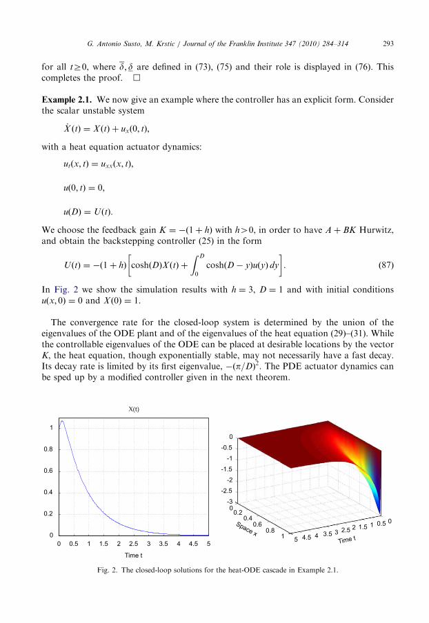
Example 2.1. We now give an example where the controller has an explicit form. Considerthe scalar unstable system

_X !t" % X !t" & ux!0; t";

with a heat equation actuator dynamics:

ut!x; t" % uxx!x; t";

u!0; t" % 0;

u!D" % U!t":

We choose the feedback gain K % '!1& h" with h40, in order to have A& BK Hurwitz,and obtain the backstepping controller (25) in the form

U!t" % '!1& h" cosh!D"X !t" &Z D

0cosh!D' y"u!y" dy

! ": !87"

In Fig. 2 we show the simulation results with h % 3, D % 1 and with initial conditionsu!x; 0" % 0 and X !0" % 1.

The convergence rate for the closed-loop system is determined by the union of theeigenvalues of the ODE plant and of the eigenvalues of the heat equation (29)–(31). Whilethe controllable eigenvalues of the ODE can be placed at desirable locations by the vectorK, the heat equation, though exponentially stable, may not necessarily have a fast decay.Its decay rate is limited by its first eigenvalue, '!p=D"2. The PDE actuator dynamics canbe sped up by a modified controller given in the next theorem.

ARTICLE IN PRESS

0 0.5 1 1.5 2 2.5 3 3.5 4 4.5 50

0.2

0.4

0.6

0.8

1

X(t)

0-0.5

-1-1.5

-2-2.5

-300.2

0.40.6

0.81

Space x5 4.5 4 3.5 3 2.5 2 1.5 1 0.5 0

Time t

Time t

Fig. 2. The closed-loop solutions for the heat-ODE cascade in Example 2.1.

G. Antonio Susto, M. Krstic / Journal of the Franklin Institute 347 (2010) 284–314 293

Theorem 2.2. Consider a closed-loop system consisting of the plant (21)–(24) and the controllaw

U!t" % f!D"X !t" &Z D

0C!D; y"u!y; t" dy; !88"

where

f!x" % KM!x" &Z D

0k!x; y"KM!y" dy; !89"

C!x; y" % k!x; y" & KM!x' y"B'Z x

y

k!x; x"f!x' y"Bdx; !90"

k!x; y" % 'cyI1!

'''''''''''''''''''''c!x2 ' y2"

p"'''''''''''''''''''''

c!x2 ' y2"p ; c40; !91"

and I1 denotes the modified Bessel function of order one. For all initial conditions such thatux!x; 0" is square integrable in x and compatible with the control law (88), the closed-loopsystem has a unique classical solution and its eigenvalues are given by

eigfA& BKg [ eig 'c'p2n2

D2; n % 1; 2; . . .

% &: !92"

Proof. The proof is developed in the same manner as the correspondent proof in [7].Consider a second, invertible change of variables

z!x; t" % w!x; t" 'Z x

0k!x; y"w!y; t" dy; !93"

which aims to map system (28)–(31) into a new target system:

_X !t" % !A& BK"X !t" & Bzx!0; t"; !94"

zt!x; t" % zxx!x; t" ' cz!x; t"; !95"

z!0; t" % 0; !96"

z!D; t" % 0: !97"

It was shown in [14,11] that the kernel function k!x; y" must satisfy the PDE:

kxx!x; y" ' kyy!x; y" % ck!x; y"; !98"

k!x; x" % 'c

2x; !99"

k!x; 0" % 0: !100"


The solution to Eq. (98)–(100) is given by Eq. (91). Taking the composition of the twobackstepping transformation (27) and (93), we obtain that

z!x" % u!x" 'Z x

0KM!x' y"Bu!y" dy' KM!x"X '

Z x

0k!x; y"u!y" dy

&Z x

0k!x; y"KM!y" dyX &

Z x

0k!x; y"

Z y

0KM!y' x"u!x" dx dy: !101"

Setting x % D, employing the boundary conditions u!D; t" % U!t", z!D; t" % 0, and thecalculus formula for changing the order of integration

Z x

0

Z y

0f !x; y; x" dx dy %

Z x

0

Z x

xf !x; y; x" dy dx; !102"

yields to the controller (88)–(90). With a calculation of the eigenvalues of Eqs. (94)–(97),we get the set (92). &

3. Robustness to diffusion uncertainty

We study the robustness of the controller (25) to perturbations in the diffusioncoefficient. Consider the following system:

_X !t" % AX !t" & Bux!0; t"; !103"

ut!x; t" % !1& e"uxx!x; t"; !104"

ux!0; t" % 0; !105"

u!D; t" %Z D

0m!D' y"u!y; t" dy& KM!D"X !t"; !106"

where e represents a perturbation in the diffusion coefficient of the heat PDE.The perturbation e can be either positive or negative, but it has to be small.

Theorem 3.1. Consider the closed-loop system consisting of the plant (103)–(106) andthe control law (25). There exists a sufficiently small e)40 such that, for all e 2 !'e); e)",the closed-loop system has a unique classical solution for all compatible initial conditionsu!x; 0" such that ux!x; 0" is square integrable in x, and is exponentially stable in the sense ofthe norm

!jX !t"j2 & Ju!t"J2 & Jux!t"J2"1=2: !107"

Proof. By differentiating the transformation

w!x; t" % u!x; t" 'Z x

0m!x' y"u!y; t" dy' KM!x"X !t"; !108"

and substituting into Eqs. (103)–(106), it can be verified that

_X !t" % !A& BK"X !t" & Bwx!0; t"; !109"

wt!x; t" % !1& e"wxx!x; t" & eKM!x"#!A& BK"X !t" & Bwx!0; t"$; !110"


w!0; t" % 0; !111"

w!D; t" % 0: !112"

Consider again the Lyapunov function (53). The derivative of V along the solutions ofsystem (109)–(112) is

_Vr'lmin!Q"

2jX j2

&2jPBj2

lmin!Q"wx!0"2 ' a!1' jej"JwxJ2 ' b!1' jej"JwxxJ2

& eaZ D

0w!x"KM!x" dx#!A& BK"X !t" & Bwx!0"$

' ebZ D

0wxx!x"KM!x" dx#!A& BK"X !t" & Bwx!0"$ !113"

r'lmin!Q"

4jX j2 ' a'

1&D

D

b

2

# $JwxJ2

'b

2'

2jPBj2

lmin!Q"' jej!a& b"

! "wx!0"2 '

b

2JwxxJ2

& ajej 1& 4Jm1J& ajej8Jm2J2

lmin!Q"

% &JwxJ2

& bjej 1& Jm1J& bjej2Jm2J2

lmin!Q"

% &JwxxJ2; !114"

where

m1!x" % KM!x"B; !115"

m2!x" % jKM!x"j: !116"

In the second inequality we have split the term bJwxxJ2 in half, used the inequality (78), andemployed Young’s and Poincar!e inequalities. Choosing for example

a %1&D

D

8jPBj2

lmin!Q"; !117"

b %8jPBj2

lmin!Q"!118"

it is possible to select jej sufficiently small to achieve negative definiteness of _V . &

4. Observer for the ODE-heat cascade with Neumann measurement

Consider the cascade depicted in Fig. 3 and governed by the equations

Y !t" % ux!0; t"; !119"

ut!x; t" % uxx!x; t"; !120"


u!0; t" % 0; !121"

u!D; t" % CX !t" !122"

_X !t" % AX !t" & BU!t"; !123"

that is, the case where an ODE system has a diffusive sensor acting on the output mapCX !t", with Neumann measurement ux!0; t". We now present an observer, inspired by [15],which compensates the sensor dynamics and guarantees exponential stability of the errorsystem.

Theorem 4.1. The observer

ut!x; t" % uxx!x; t" & CM!x"#Y !t" ' ux!0; t"$; !124"

u!0; t" % 0; !125"

u!D; t" % CX !t"; !126"

_X !t" % AX !t" & BU !t" &M!D"L#Y !t" ' ux!0; t"$; !127"

where L is chosen such that !A' LC" is Hurwitz, guarantees that the error system

~ut!x; t" % ~uxx!x; t" ' CM!x"L ~ux!0; t"; !128"

~u!0; t" % 0; !129"

~u!D; t" % C ~X !t"; !130"

_~X !t" % A ~X !t" 'M!D"L ~ux!0; t"; !131"

where ~X % X ' X and ~u % u' u, is exponentially stable in the sense of the norm

j ~X !t"j2 &Z D

0

~ux!x; t"2 dx# $1=2

: !132"

Proof. Consider the backstepping transformation

~w!x" % ~u!x" ' CM!x"M!D"'1 ~X !133"

to map the error system into a new PDE system. Differentiating the transformation (133)with respect to time and space

~wt!x" % ~ut!x" ' CM!x"M!D"'1A ~X !t" & CM!x"L ~ux!0"; !134"

ARTICLE IN PRESS

Fig. 3. The cascade of the ODE plant and the heat equation PDE dynamics.


~wx!x" % ~ux!x" ' CM 0!x"M!D"'1 ~X !t"; !135"

~wxx!x" % ~uxx!x" ' CM!x"AM!D"'1 ~X !t": !136"

Then evaluating (135) in x % 0 and using the initial condition

M 0!0" % In !137"

and the plant equation (131), we obtain

_~X !t" % !A'M!D"LCM!D"'1" ~X !t" 'M!D"L ~wx!0; t": !138"

Summarizing we get the following PDE:

~wt!x; t" % ~wxx!x; t"; !139"

~w!0; t" % 0; !140"

~w!D; t" % 0; !141"

_~X !t" % !A'M!D"LCM!D"'1" ~X !t" &M!D"L ~wx!0; t": !142"

The matrix #A'M!D"LCM!D"'1$ is Hurwitz, which can be seen with a similaritytransformation M!D", which commutes with A thanks to the properties of the matrixexponential. Now consider the Lyapunov function

V % ~XTM!D"'TPM!D"'1 ~X &

a

2J ~wJ2 &

b

2J ~wJ2; !143"

where the matrix P % PT40 is the solution to the Lyapunov equation

P!A' LC" & !A' LC"TP % 'Q !144"

for some Q % QT40, and the parameters a40 and b40 will be chosen later. From thispoint on, we develop the proof using similar ideas as in the proof of Theorem 2.1. We firstcompute the time-derivative of function V,

_V % ' ~XTM!D"'TQM!D"'1 ~X & 2 ~X

TPL ~wx!0"

&a

2

Z D

0

d

dt! ~w!x"2" dx&

b

2

Z D

0

d

dt! ~wx!x"2" dx: !145"

Using the boundary conditions (140)–(141) we get

_V % ' ~XTM!D"'TQM!D"'1 ~X & 2 ~X

TPL ~wx!0" ' aJ ~wxJ2 ' bJ ~wxxJ2r

'lmin!Q"

2j ~X j2 &

2jM!D"'TPLjlmin!Q"

~wx!0"2 ' aJ ~wxJ2 ' bJ ~wxxJ2; !146"

where we had applied Young’s Inequality. We now use inequality (78), which gives us

'J ~wxxJ2r1&D

DJ ~wxJ2 ' ~wx!0"2; !147"


hence we get

_Vr'lmin!Q"

2j ~X j2 ' !b'

2jM!D"'TPLjlmin!Q"

" ~wx!0"2 ' a' b1&D

D

# $J ~wxJ2: !148"

As was done in the proof of Theorem 2.1, taking a and b sufficiently large and thenapplying again Poincar!e’s inequality, we get that _Vr' nV for some n40. This impliesthat the target system ! ~X ; ~w" is exponentially stable at the origin. From the backsteppingtransformation (133) we get exponential stability of the error system (128)–(131) in thesense of the norm

j ~X !t"j2 & J ~ux!t"J2rdde'bt!j ~X !0"j2 & J ~ux!0"J2" !149"

for all tZ0. &

The observer presented in this section has the same structure of the observer proposed in[7] for the cascade

Y !t" % u!0; t"; !150"

ut!x; t" % uxx!x; t"; !151"

ux!0; t" % 0; !152"

u!D; t" % CX !t"; !153"

_X !t" % AX !t" & BU!t": !154"

The observer proposed in [7] is actually

ut!x; t" % uxx!x; t" & CM1!x"L#Y !t" ' u!0; t"$; !155"

ux!0; t" % 0; !156"

u!D; t" % CX !t"; !157"

_X !t" % AX !t" & BU !t" &M1!D"L#Y !t" ' u!0; t"$; !158"

where

M1!x" % #I 0$e#0I

A0$x

I

0

! ": !159"

The transformation (133) used to study the two observers is the same in both proofs ofstability; this similarity is possible thanks to the swapping between the initial conditions offunction M and M1 in the two problems. Note that M!0" % M1

0 !0" % I andM 0!0" % M1!0" % 0.

Example 4.1. Consider the scalar unstable system

_X !t" % X !t" &U!t"; !160"

with a heat equation sensor dynamics:

Y !t" % u!0; t"; !161"


ut!x; t" % uxx!x; t"; !162"

ux!0; t" % 0; !163"

u!D; t" % X !t": !164"

In this case we have that M!x" % coshx and the backstepping observer proposed is

ut!x; t" % uxx!x; t" & !1& g"coshx#Y !t" ' ux!0; t"$; !165"

u!0; t" % 0; !166"

u!D; t" % X !t"; !167"

_X !t" % X !t" &U!t" & !1& g"coshD#Y !t" ' ux!0; t"$; !168"

where we choose L % 1& g, g40, in order to have A' LC Hurwitz. In Fig. 4 we showsimulation results for g % 1, D % 1, U!t" % 0:05sin!15t" and with initial conditionsu!x; 0" % '!3=D"x and X !0" % '10, whereas the observer initial conditions areX !0" % 0; u!x; 0" * 0.

5. The diffusion–counterconvection PDE: controller and observer design

We now study a more complicated parabolic PDE, incorporating both the effects ofdiffusion and of convection,

_X !t" % AX !t" & Bu!0"; !169"

ut % uxx ' bux; !170"

ux!0" % 0; !171"

u!D" % U!t": !172"

For b40 the convection effect opposes the propagation of the control input U!t" towards theODE plant. We refer to this effect as counter-convection. The problem considered in this

ARTICLE IN PRESS

0 0.5 1 1.5 2 2.5 3-12

-10

-8

-6

-4

-2

0

2

Time t

2

0

-2

-4

-6

-8

-10

-121

0.80.6

0.40.2

0 0

Space x0.5 1 1.5 2 2.5 3

Time t

Fig. 4. The error system evolution for Example 4.1. Left: ~X !t". Right: ~u!t".


section is a generalization of the problem considered in [7] in which the system (169)–(172) wasstudied for b % 0. We provide results which recover those presented in [7] for b % 0.

Theorem 5.1. Consider a closed-loop system consisting of the plant (169)–(172) and thecontrol law

U!t" %Z D

0Km!D' y"u!y; t" dy& KM!D"X !t"; !173"

where

m!s" % 'b

2ebs &

Z s

0ebsKM!s' s"Bds; !174"

M!x" % Ib

2I

! "e#

0I

AbI$x

I

0

! ": !175"

For any initial condition such that u!x; 0" is square integrable in x and compatible with thecontrol law (173), the closed-loop system has a unique classical solution and is exponentiallystable in the sense of the norm

jX !t"j2 &Z D

0u!x; t"2 dx

# $1=2

: !176"

Proof. We employ again the backstepping transformation (27) to map the original system(169)–(172) into the target one

_X !t" % !A& BK"X !t" & Bw!0"; !177"

wt % wxx ' bwx; !178"

wx!0" %b

2w!0"; !179"

w!D" % 0: !180"

As done in the previous proof of stabilization, we first compute the derivatives wx, wxx andwt in order to derive the kernel functions q!x; y" and g!x"; comparing the expressionsobtained with Eqs. (177)–(179) we get the following sets of conditions to be satisfied:

g!0" % 0; !181"

g0!0" % Kb

2; !182"

g00!x" % bg0!x" & g!x"A; !183"

that is, a second order ODE in x, and

kxx ' kyy % b#kx & ky$; !184"

ky!x; 0" % 'bk!x; 0" ' g!x"B; !185"

k!x;x" % 'b

2; !186"


which is a hyperbolic second order PDE. The ODE (181)–(183) is solved by

g!x" % KM!x"; !187"

M!x" % Ib

2I

! "e#

0I

AbI$x

I

0

! ": !188"

In order to solve the PDE (184)–(186) we introduce a change of variables

k!x; y" % p!x; y"e!b=2"!x'y": !189"

Differentiating (189) twice with respect to x and twice with respect to y we obtain a newPDE

pxx % pyy; !190"

py!x; 0" % 'b

2p!x; 0" ' g!x"Be'!b=2"x; !191"

p!x; x" % 'b

2: !192"

Eq. (190) has a general solution of the form

p!x; y" % f!x' y" & c!x& y": !193"

Using the boundary condition p!x;x" % 'b=2 we get

f!0" & c!2x" % 'b

2: !194"

Without loss of generality we can set c * 0 and f!0" % 'b=2. Hence we have that

p!x; y" % f!x' y": !195"

Substituting this into the PDE (190)–(192) we get the following differential equation:

'f0!x" % 'b

2f!x" ' KM!x"Be'!b=2"x: !196"

Applying to (196) the Laplace transform with respect to x we obtain

f!s" %1

s'b

2

'b

2& KM s&

b

2

# $B

! ": !197"

Anti-transforming this expression we get

f!z" % 'b

2e!b=2"z & !f!g"!z"; !198"

where

f !z" % e!b=2"z; !199"

g!z" % KM!z"Be'!b=2"z; !200"

and hence

f!z" % 'b

2e!b=2"z &

Z z

0ebsKM!z' s"Be'!b=2"z ds: !201"


We finally obtain the solution for k!x; y" as

k!x; y" % f!x' y"e!b=2"!x'y" % 'b

2eb!x'y" &

Z x'y

0ebsKM!x' y' s"Bds !202"

% m!x' y": !203"

In the same manner we get the inverse transformation

u!x" % w!x" &Z x

0Kn!x' y"w!y" dy& KN!x"X !t"; !204"

where

N!s" % #I 0$e#0I

A&BKbI $s I

0

! "; !205"

n!s" % 'b

2e2bs

Z s

0N!s"Be2bse!b=2"!s's" ds: !206"

Consider now the Lyapunov function

V % XTPX & 12JwJ

2; !207"

where P % PT40 is the solution of the Lyapunov equation

P!A& BK" & !A& BK"TP % 'Q !208"

for some Q % QT40. Differentiating (207) with respect to time, exploiting the boundaryconditions (179) and (180), and applying Poincar!e’s inequality we get

_Vr' lmin!Q"jX j2 '1

4D2JwJ2r' bV ; !209"

where

b % min lmin!Q";1

4D2

% &: !210"

Applying Cauchy–Schwartz and Young’s inequalities we obtain the bounds

JwJ2ra1JuJ2 & a2jX j2; !211"

JuJ2rb1JwJ2 & b2jX j2; !212"

where

a1 % 3!1&DJmJ2"; !213"

a2 % 3JKMJ2; !214"

b1 % 3!1&DJnJ2"; !215"

b2 % 3JKNJ2: !216"

Exploiting (211) and (212) we get

d!JuJ2 & JXJ2"rVrd!JuJ2 & JXJ2"; !217"


where

d % maxa12; lmax!P" &

a22

n o; !218"

d %maxfb1; b2 & 1gmin 1

2 ; lmin!P"( ) : !219"

Combining the last inequality with (210) yields to

jX !t"j2 & Ju!t"J2r dde'bt!jX !0"j2 & Ju!0"J2" !220"

for all tZ0. &

It is interesting to analyze the results we had achieved in this section by comparison withthe case without counter-convection, which was studied in [7]. With b % 0 we get

M#b%0$!s" % #I 0$e#0I

A0 $s

I

0

! "; !221"

N#b%0$!s" % #I 0$e#0I

A&BK0 $s I

0

! "; !222"

m#b%0$!s" %Z s

0KM #b%0$!s' s"Bds; !223"

n#b%0$!s" %Z s

0KM #b%0$!s' s"Bds; !224"

which are exactly the same functions used in the controller presented in [7].The generalization that we have obtained here is thus consistent with [7].For the diffusion–counterconvection PDE we study the dual case where the PDE is in

the sensor dynamics,

Y !t" % u!0; t"; !225"

ut!x; t" % uxx!x; t" ' bux!x; t"; !226"

ux!0; t" % 0; !227"

u!D; t" % CX !t"; !228"

_X !t" % AX !t" & BU!t": !229"

Theorem 5.2. The observer

ut!x; t" % uxx!x; t" ' bux!x; t" & CM!x"L#Y !t" ' u!0; t"$; !230"

ux!0; t" % 'b

2#Y !t" ' u!0; t"$; !231"

u!D; t" % CX !t"; !232"


_X !t" % AX !t" & BU !t" &M!D"L#Y !t" ' u!0; t"$; !233"

where L is chosen such that A' LC is Hurwitz and matrix function M!(" is defined by (188),guarantees that the error system

~ut!x; t" % ~uxx!x; t" ' b ~ux!x; t" ' CM!x"L ~u!0; t"; !234"

~ux!0; t" % 'b

2~u!0; t"; !235"

~u!D; t" % C ~X !t"; !236"

_~X !t" % A ~X !t" 'M!D"L ~u!0; t"; !237"

where ~X % X ' X and ~u % u' u, is exponentially stable in the sense of the norm

j ~X !t"j2 &Z D

0

~u!x; t"2 dx# $1=2

: !238"

Proof. We introduce the transformation

~w!x; t" % ~u!x; t" ' CM!x"M!D"'1 ~X !t"; !239"

which is actually the same the one used in proof of Theorem 4.1, but with a differentfunction M!x". Evaluating (239) at x % 0 and D we get

~w!0; t" % ~u!0; t" ' CM!D"'1 ~X !t"; !240"

~w!D; t" % 0: !241"

Exploiting (240) and the ODE system equation (237) we obtain

_~X !t" % #A'M!D"LCM!D"'1$ ~X !t" 'M!D"L ~w!0": !242"

We now proceed to differentiate (239) with respect to x:

~wx!x; t" % ~ux!x; t" ' CM 0!x"M!D"'1 ~X !t": !243"

Evaluating (243) at the boundary x % 0 and making use of the initial conditionM!0" % !b=2"I and the boundary condition (235), we get

~wx!0; t" %b

2~u!0; t": !244"

Differentiating again with respect to x we get:

~wxx!x; t" % ~uxx!x; t" ' bCM 0!x"M!D"'1 ~X !t" ' CM!x"AM!D"'1 ~X !t"; !245"


where we had used the equation M 00!x" % bM 0!x" &M!x"A. Differentiating thetransformation (239) with respect to time we obtain

~wt!x; t" % ~ut!x; t"

' CM!x"M!D"'1 _~X !t"% ~uxx!x; t" ' b ~ux!x; t" ' CM!x"L ~u!0; t"

' CM!x"M!D"'1A ~X !t" & CM!x"L ~u!0; t"% ~wxx!x; t" ' b ~wx!x; t"; !246"

where we had used Eqs. (237), (234), (243) and (245). Summarizing, we have obtained thefollowing PDE–ODE system:

~wt!x; t" % ~wxx!x; t" ' b ~wx!x; t"; !247"

~wx!0; t" %b

2~w!0; t"; !248"

~w!D; t" % 0; !249"

_~X !t" % #A'M!D"LCM!D"'1$ ~X !t" 'M!D"L ~w!0; t": !250"

We now consider the Lyapunov function

V % ~XTM!D"'TPM!D"'1 ~X & 1

2J ~wJ2; !251"

where P % PT40 is the solution to the Lyapunov equation

P!A' LC" & !A' LC"TP % 'Q !252"

for some Q % QT40. Differentiating (251) with respect to time and exploiting theboundary conditions (247) and (248) we get

_V % ' ~XTM!D"'TQM!D"'1 ~X ' ~w!0" ~wx!0" ' JwxJ2

' 2 ~XTM!D"'TQM!D"'1 ~X &

b

2~w!0"2: !253"

Using the Poincar!e inequality and the boundary condition w!D" % 0 we get

_Vr' lmin!Q"j ~X j2 '1

4D2J ~wJ2r' ZV ; !254"

where

Z % min lmin!Q";1

4D2

% &: !255"

From the transformation (239) we derive the following inequalities:

J ~wJ2rJ ~uJ2 & bj ~X j2; !256"

J ~uJ2rJ ~wJ2 & bj ~X j2; !257"

with

b % JCMM!D"'1J2: !258"


Thus

d!j ~X j2 & J ~uJ2" rVr d!j ~X j2 & J ~uJ2"; !259"

where

d % maxflmax!P" & b; 12g; !260"

d %minf12 ; lmin!P"gmax 1; b& 1

( ) : !261"

Combining (259) with (254) yields

j ~X !t"j2 & J ~ux!t"J2rdde'Zt!j ~X !0"j2 & J ~ux!0"J2" !262"

for all tZ0. &

As we did for the full-state control problem, it is interesting to compare the results thatwe have obtained for to the corresponding case with b % 0, that is, the purely diffusivePDE, without counter-convection. For b % 0 the observer (230)–(233) becomes

ut!x; t" % uxx!x; t" & CM!x"L#Y !t" ' u!0; t"$; !263"

ux!0; t" % 0; !264"

u!D; t" % CX !t"; !265"

_X !t" % AX !t" & BU !t" &M!D"L#Y !t" ' u!0; t"$; !266"

which is exactly the same observer presented in [7] for the following problem:

Y !t" % u!0; t"; !267"

ut!x; t" % uxx!x; t"; !268"

ux!0; t" % 0; !269"

u!D; t" % CX !t"; !270"

_X !t" % AX !t" & BU!t": !271"

ARTICLE IN PRESS

Fig. 5. The cascade of a wave PDE with an ODE plant.


6. The wave-ODE cascade with Neumann interconnection

Consider the following system:

utt!x; t" % uxx!x; t"; !272"

u!0; t" % 0; !273"

ux!D; t" % U!t"; !274"

_X !t" % AX !t" & Bux!0; t"; !275"

which is depicted in Fig. 5. We are looking for a backstepping transformation that makesthe system (272)–(275) behave as the following target system:

wtt!x; t" % wxx!x; t"; !276"

w!0; t" % 0; !277"

wx!D; t" % 'cwt!D; t"; c40; !278"

_X !t" % !A& BK"X !t" & Bwx!0; t"; !279"

where K is such that !A& BK" is Hurwitz.We postulate the backstepping transformation

w!x; t" % u!x; t" 'Z x

0k!x; y"u!y; t" dy'

Z x

0l!x; y"ut!y; t" dy' g!x"X !t"; !280"

which is inspired by the construction in [16]. As done in the previous problems, wedifferentiate the transformation (280) to gather conditions that the unknown functionsmust satisfy. In order to verify the wave equation (276) we must differentiate twice withrespect to time and to space. We first differentiate with respect to time1:

wt!x" % ut!x" 'Z x

0k!x; y"ut!y" dy' l!x;x"ux!x" & l!x; 0"ux!0" & ly!x; x"u!x"

' g!x"Bux!0" ' g!x"AX 'Z x

0lyy!x; y"u!y" dy; !281"

where we had used (276), the boundary condition (277) and integrated twice by parts.Differentiating again with respect to time:

wtt!x" % uxx!x" ' k!x;x"ux!x" & k!x; 0"ux!0" & ky!x;x"u!x"

'Z x

0kyy!x; y"ut!y" dy& l!x;x"uxt!x" & ly!x;x"ut!x" ' g!x"A _X

&'Z x

0lyy!x; y"ut!y" dy& #l!x; 0" ' g!x"B$uxt!0": !282"

ARTICLE IN PRESS

1We drop the dependence on time of state variables w!x; t" and u!x; t" for the sake of compact notation.


Now we proceed differentiating with respect to space:

wx!x" % ux!x" ' k!x;x"u!x" 'Z x

0kx!x; y"u!y" dy' l!x;x"ut!x"

'Z x

0lx!x; y"ut!y" dy' g!x"0X !t"; !283"

wxx!x" % uxx!x" 'd

dx#k!x;x"$u!x" ' k!x;x"ux!x" ' kx!x;x"u!x"

'Z x

0kxx!x; y"u!y" dy'

d

dx#l!x;x"$ut!x" ' l!x;x"utx!x" ' lx!x;x"ut!x"

'Z x

0lxx!x; y"ut!y" dy' g!x"00X !t": !284"

Matching (282)–(284) yields to the following PDEs:

lxx % lyy; !285"

l!x; 0" % g!x"B; !286"

l!x; x" % 0; !287"

kxx % kyy; !288"

k!x; 0" % g!x"AB; !289"

k!x;x" % 0; !290"

g!x"00 % g!x"A2; !291"

g!0" % 0; !292"

g!0"0 % K : !293"

Exploiting the previous we obtain the following expression for the unknown functions:

g!x" % KM!x" !294"

% K #0 I $e#0I

A2

0 $xI

0

! "; !295"

l!x; y" % m!x' y"; !296"

k!x; y" % m!x' y"; !297"

m!s" % g!s"B; !298"

m!s" % g!s"AB: !299"


The explicit expression for the controller is derived from (278). Evaluating w!D; t" from(281) and wx!D; t" and exploiting (283) we get

U!t" % c#KBu!D; t" ' ut!D; t"$ & r!D"X !t"

&Z D

0r!D' x"#ABu!x; t" & But!x; t"$ dx; !300"

where the function r!s" is defined by

r!s" % K #0 I $e#0I

A2

0 $scA

I

! ": !301"

In the same manner in which we derive the direct backstepping transformation, we alsoderive the inverse transformation

u!x" % w!x" &Z x

0f!x' y"w!y" dy&

Z x

0n!x' y"wt!y" dy& c!x"X ; !302"

where

c!x" % KN!x"; !303"

N!x" % #0 I $e#0I

!A&BK"20 $x I

0

! "; !304"

n!s" % c!s"B; !305"

f!s" % c!s"AB: !306"

Having designed the controller we now show that it guarantees exponential stability tothe original system.

Theorem 6.1. Consider the closed-loop system consisting of the plant (272)–(275) andthe control law (300). For any initial conditions such that ux!x; 0" and ut!x; 0" are squareintegrable in x and compatible with (300), the closed-loop system has a unique solution that isexponentially stable in the sense of the norm

jX !t"j2 &Z D

0ux!x; t"2 dx&

Z D

0ut!x; t"2 dx

# $1=2

: !307"

Proof. We start by introducing the system norms

O!t" % Jux!t"J2 & Jut!t"J2 & jX !t"j2; !308"

X!t" % Jwx!t"J2 & Jwt!t"J2 & jX !t"j2: !309"

To prove the stability of the closed-loop system (272)–(275) and (300) we employ theLyapunov function

V !t" % X !t"TPX !t" & aE!t"; !310"


where the matrix P % PT40 is the solution to the Lyapunov equation

P!A& BK" & !A& BK"TP % 'Q !311"

for some Q % QT40, the design parameter a40 is to be chosen later and the function E!t"is defined by

E!t" %1

2!Jwx!t"J2 & Jwt!t"J2" & d

Z D

0!1& y"wx!y; t"wt!y; t" dy; !312"

where d40 is also a parameter to be chosen later. We observe that

y1XrVry2X; !313"

where

y1 % min lmin!P";a

2#1' d!1&D"$

n o; !314"

y2 % min lmax!P";a

2#1& d!1&D"$

n o: !315"

We choose

0odo 1

1&D!316"

in order to ensure that y1 and y2 are non-negative and so the Lyapunov function V ispositive semi-definite. Next, we compute the time derivative of E!t"

_E !t" % 'd2#Jwx!t"J2 & Jwt!t"J2 & wx!0; t"2$

&d2!1&D"#wt!D; t"2 & wx!D; t"2$ & wx!D; t"wt!D; t": !317"

We substitute the feedback law wx!D; t" % 'cwt!D; t" and get

_E !t" % 'd2#Jwx!t"J2 & Jwt!t"J2 & wx!0; t"2$ & ' c' d

1&D

2!1& c2"

! "

|******************{z******************}b

wt!D; t"2: !318"

Choosing now

do 2c

!1&D"!1& c2"!319"

we have that b40. We now compute the derivative of V !t":

_V !t" % 'X !t"TQX !t"

& 2X !t"TPBwx!0; t" & a _E !t"r'lmin!Q"

2jX !t"j2

&2jPBj2

lmin!Q"' a

d2

! "wx!0; t"2 ' a

d2#Jwx!t"J2 & Jwt!t"J2$ ' abwt!D; t"2: !320"


To have _V !t"o0 we choose

aZ4jPBj2

dlmin!Q": !321"

We now obtain

_V !t"r'lmin!Q"

2jX !t"j2 ' a

d2#Jwx!t"J2 & Jwt!t"J2$ !322"

r' ZV !t"; !323"

where

Z %min

lmin!Q"2

;ad2

% &

y2: !324"

Thus we arrive at the estimate

V !t"re'ZtV !0": !325"

To prove stability of the closed-loop system in its original variables !u;X ", from (325) weprovide inequalities relating the variables u!x; t" and w!x; t". From the inversetransformation (302) we obtain that

ux!x; t" % wx!x; t" &Z x

0f0!x' y"w!y" dy&

Z x

0n0!x' y"wt!y" dy& c!x"0X !t"; !326"

ut!x; t" % wt!x; t" &Z x

0f!x' y"wt!y" dy&

Z x

0n0!x' y"w!y" dy

& c!x"!A& BK"X !t": !327"

Applying Poincar!e, Young’s and the Cauchy–Schwartz inequality, we get

Jux!t"J2ra1Jwx!t"J2 & a2Jwt!t"J2 & a3jX !t"j2; !328"

Jut!t"J2rb1Jwx!t"J2 & b2Jwt!t"J2 & b3jX !t"j2; !329"

where

a1 % 4!1& 4D3Jf0J2"; !330"

a2 % 4DJn0J2; !331"

a3 % 4Jc0J2; !332"

b1 % 4Jn0J2; !333"

b2 % 4!1& 4D3JfJ2"; !334"

b3 % 4Jc!A& BK"J2: !335"


Applying (328) and (329) we obtain

O!t"ry4X!t"; !336"

where

y4 % maxfa1 & b1; a2 & b2; a3 & b3 & 1g: !337"

With the help of Eqs. (281) and (283) and applying again Poincar!e, Young’s and theCauchy–Schwartz inequalities, we obtain the following inequalities:

Jwx!t"J2ra1Jux!t"J2 & a2Jux!t"J2 & a3jX !t"j2; !338"

Jwt!t"J2rb1Jux!t"J2 & b2Jux!t"J2 & b3jX !t"j2; !339"

where

a1 % 4!1& 4D3Jm0J2"; !340"

a2 % 4DJm0J2; !341"

a3 % 4Jf0J2; !342"

b1 % 4DJm0J2; !343"

b2 % 4!1& 4JmJ2"; !344"

b3 % 4JfAJ2: !345"

Applying (338) and (339) we obtain

y3X!t"rO!t"; !346"

where

y3 %1

maxfa1 & b1; a2 & b2; a3 & b3 & 1g: !347"

With the help of inequalities (313), (325), (336) and (346) we get

O!t"r y1y3y2y4

O!0"e'Zt; !348"

that is,

Jux!t"J2 & Jux!t"J2 & jX !t"j2r y1y3y2y4

e'Zt#Jux!0"J2 & Jut!0"J2 & jX !0"j2$: & !349"

7. Conclusions

In this article we have developed explicit controllers and observers for PDE–ODEcascades involving heat and wave equation, extending the results in [7,8]. Many openproblems in PDE–ODE cascades remain. For example, the system

_X !t" % AX !t" & B0u!0; t" & B1ux!0; t"; !350"


ut!x; t" % uxx!x; t" ' bux!x; t" & lu!x; t"; !351"

ux!0; t" % qu!0; t" &HX !t"; !352"

u!D; t" % U!t"; !353"

contains several interesting problems, including one where u!0; t" and ux!0; t" simulta-neously appear in the ODE, and an even more interesting one where the ‘‘interconnection’’between the PDE and the ODE is not one-directional (as in this paper and in [7,8]), butwhere the ODE acts back on the PDE, such as, for example, the term HX !t" in theboundary condition (353).

References

[1] O.-M. Aamo, A. Smyshlyaev, M. Krstic, Boundary control of the linearized Ginzburg–Landau model ofvortex shedding, SIAM Journal of Control and Optimization 43 (2005) 1953–1971.

[2] O.M. Aamo, A. Smyshlyaev, M. Krstic, B. Foss, Stabilization of a Ginzburg-Landau model of vortexshedding by output-feedback boundary control, IEEE Transactions on Automatic Control 52 (2007)742–748.

[3] Z. Artstein, Linear systems with delayed controls: a reduction, IEEE Transactions on Automatic Control 27(1982) 869–879.

[4] A. Balogh, M. Krstic, Infinite-dimensional backstepping-style feedback transformations for a heat equationwith an arbitrary level of instability, European Journal of Control 8 (2002) 165–177.

[5] A. Balogh, M. Krstic, Stability of partial difference equations governing control gains in infinite-dimensionalbackstepping, Systems and Control Letters 51 (2004) 151–164.

[6] M. Krstic, Lyapunov tools for predictor feedbacks for delay systems: inverse optimality and robustness todelay mismatch, Automatica 44 (2008) 2930–2935.

[7] M. Krstic, Compensating actuator and sensor dynamics governed by diffusion PDEs, Systems & ControlLetters 58 (2009) 372–377.

[8] M. Krstic, Compensating a string PDE in the actuation or in sensing path of an unstable ODE, IEEETransactions on Automatic Control 54 (2009) 1362–1368.

[9] M. Krstic, Delay Compensation for Nonlinear, Adaptive, and PDE Systems, Birkhauser, 2009.[10] M. Krstic, A. Smyshlyaev, Backstepping boundary control for first order hyperbolic PDEs and application to

systems with actuator and sensor delays, Systems & Control Letters 57 (2008) 750–758.[11] M. Krstic, A. Smyshlyaev, Boundary Control of PDEs: A Course on Backstepping Designs, SIAM, 2008.[12] W.H. Kwon, A.E. Pearson, Feedback stabilization of linear systems with delayed control, IEEE

Transactions on Automatic Control 25 (1980) 266–269.[13] A.Z. Manitius, A.W. Olbrot, Finite spectrum assignment for systems with delays, IEEE Transactions on

Automatic Control 24 (1979) 541–553.[14] A. Smyshlyaev, M. Krstic, Closed form boundary state feedbacks for a class of 1D partial integro-differential

equations, IEEE Transactions on Automatic Control 49 (12) (2004) 2185–2202.[15] A. Smyshlyaev, M. Krstic, Backstepping observers for a class of parabolic PDEs, Systems & Control Letters

54 (2005) 613–625.[16] A. Smyshlyaev, M. Krstic, Boundary control of an unstable wave equation with anti-damping on the

uncontrolled boundary, Systems & Control Letters 58 (2009) 617–623.[17] E.D. Sontag, Smooth stabilization implies coprime factorization, IEEE Transactions on Automatic Control

34 (1989) 435–443.[18] R. Vazquez, M. Krstic, A closed-form feedback controller for stabilization of the linearized 2D

Navier–Stokes Poiseuille flow, IEEE Transactions on Automatic Control 52 (2007) 2298–2312.


control of pde–ode cascades with neumann interconnectionsflyingv.ucsd.edu/papers/pdf/128.pdf ·...

Documents