control function and related methods jeff wooldridge … · control function and related methods...

CONTROL FUNCTION AND RELATED METHODS

Jeff WooldridgeMichigan State UniversityLABOUR Lectures, EIEF

October 18-19, 2011

1. Linear-in-Parameters Models: IV versus Control Functions2. Correlated Random Coefficient Models3. Nonlinear Models4. Semiparametric and Nonparametric Approaches5. Methods for Panel Data

1

1. Linear-in-Parameters Models: IV versus ControlFunctions

∙Most models that are linear are estimated using standard IV methods:

two stage least squares (2SLS) or generalized method of moments

(GMM).

∙ An alternative, the control function (CF) approach, relies on the same

kinds of identification conditions. But even in models linear in

parameters it can lead to different estimators.

2

∙ Let y1 be the response variable, y2 the endogenous explanatory

variable (EEV), and z the 1 L vector of exogenous variables (with

z1 1:

y1 z11 1y2 u1, (1)

where z1 is a 1 L1 strict subvector of z.

3

∙ First consider the exogeneity assumption

Ez′u1 0. (2)

Reduced form for y2:

y2 z2 v2, Ez′v2 0 (3)

where 2 is L 1. Write the linear projection of u1 on v2, in error form,

as

u1 1v2 e1, (4)

where 1 Ev2u1/Ev22 is the population regression coefficient. By

construction, Ev2e1 0 and Ez′e1 0.

4

Plug (4) into (1):

y1 z11 1y2 1v2 e1, (5)

where v2 is an explanatory variable in the equation. The new error, e1,

is uncorrelated with y2 as well as with v2 and z.

5

∙ Suggests a two-step estimation procedure:

(i) Regress y2 on z and obtain the reduced form residuals, v2.

(ii) Regress

y1 on z1,y2, and v2. (6)

The implicit error in (6) is ei1 1zi2 − 2, which depends on the

sampling error in 2 unless 1 0. OLS estimators from (6) will be

consistent for 1,1, and 1.

6

∙ The OLS estimates from (6) are control function estimates.

∙ The OLS estimates of 1 and 1 from (6) are identical to the 2SLS

estimates starting from (1).

∙ A test of H0 : 1 0 in the equation

yi1 zi11 1yi2 1vi2 errori

is the regression-based Hausman test for H0 : Covy2,u1 0. Is

easily made robust to heteroskedasticity of unknown form.

7

∙ The equivalence of IV and CF methods does not always. Add a

quadratic in y2:

y1 z11 1y2 1y22 u1

Eu1|z 0. (7) (8)

∙ Cannot get very far now without the stronger assumption (8).

∙ Let z2 be a (nonbinary) scalar not also in z1. Under assumption (8),

we can use, say, z22 as an instrument for y2

2. So the IVs would be

z1, z2, z22 for z1,y2,y2

2. We could also use interactions z2z1.

8

∙What does the CF approach entail? Because of the nonlinearity in y2,

the CF approach is based on the conditional mean, Ey1|z,y2, rather

than a linear projection.

∙ Therefore, we now assume

Eu1|z,y2 Eu1|v2 1v2 (9)

where

y2 z2 v2.

∙ Independence of u1,v2 and z is sufficient for the first equality. Even

under the independence assumption, linearity of Eu1|v2 is a

substantive restriction.

9

∙ Under Eu1|z,y2 1v2, we have

Ey1|z,y2 z11 1y2 1y22 1v2. (10)

A CF approach is immediate: replace v2 with v2 and use OLS on (10).

Not equivalent to a 2SLS estimate.

∙ If the assumptions hold, CF likely more efficient; it is less robust than

an IV approach, which requires only Eu1|z 0.

∙ At a minimum the CF approach requires Ev2|z 0 or

Ey2|z z2, which puts serious restrictions on y2.

10

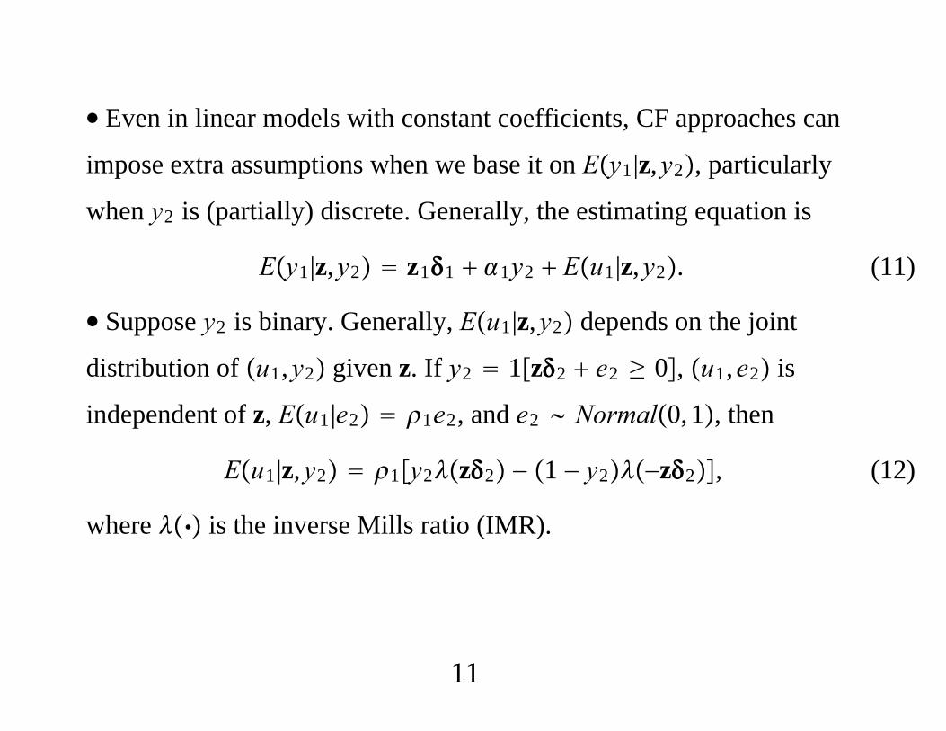
∙ Even in linear models with constant coefficients, CF approaches can

impose extra assumptions when we base it on Ey1|z,y2, particularly

when y2 is (partially) discrete. Generally, the estimating equation is

Ey1|z,y2 z11 1y2 Eu1|z,y2. (11)

∙ Suppose y2 is binary. Generally, Eu1|z,y2 depends on the joint

distribution of u1,y2 given z. If y2 1z2 e2 ≥ 0, u1,e2 is

independent of z, Eu1|e2 1e2, and e2 Normal0, 1, then

Eu1|z,y2 1y2z2 − 1 − y2−z2, (12)

where is the inverse Mills ratio (IMR).

11

∙ The CF approach is based on

Ey1|z,y2 z11 1y2 1y2z2 − 1 − y2−z2

and the Heckman two-step approach (for endogeneity, not sample

selection):

(i) Probit to get 2 and compute gri2 ≡ yi2zi2 − 1 − yi2−zi2

(generalized residual).

(ii) Regress yi1 on zi1, yi2, gri2, i 1, . . . ,N (and adjust the standard

errors).

12

∙ Consistency of the CF estimators hinges on the model for Dy2|z

being correctly specified, along with linearity in Eu1|e2. If we just

apply 2SLS directly to y1 z11 1y2 u1, it makes no distinction

among discrete, continuous, or some mixture for y2.

∙ How might we robustly use the binary nature of y2 in IV estimation?

Obtain the fitted probabilities, zi2, from the first stage probit, and

then use these as IVs (not regressors!) for yi2. Fully robust to

misspecification of the probit model, usual standard errors from IV

asymptotically valid. Efficient IV estimator if Py2 1|z z2

and Varu1|z 12.

∙ Similar suggestions work for y2 a count variable or a corner solution.

13

2. Correlated Random Coefficient Models

∙Modify the original equation as

y1 1 z11 a1y2 u1 (13)

where a1, the “random coefficient” on y2. Heckman and Vytlacil

(1998) call (13) a correlated random coefficient (CRC) model. For a

random draw i, yi1 1 zi11 ai1y2 ui1.

∙Write a1 1 v1 where 1 Ea1 is the parameter of interest.

We can rewrite the equation as

y1 1 z11 1y2 v1y2 u1

≡ 1 z11 1y2 e1. (14) (15)

14

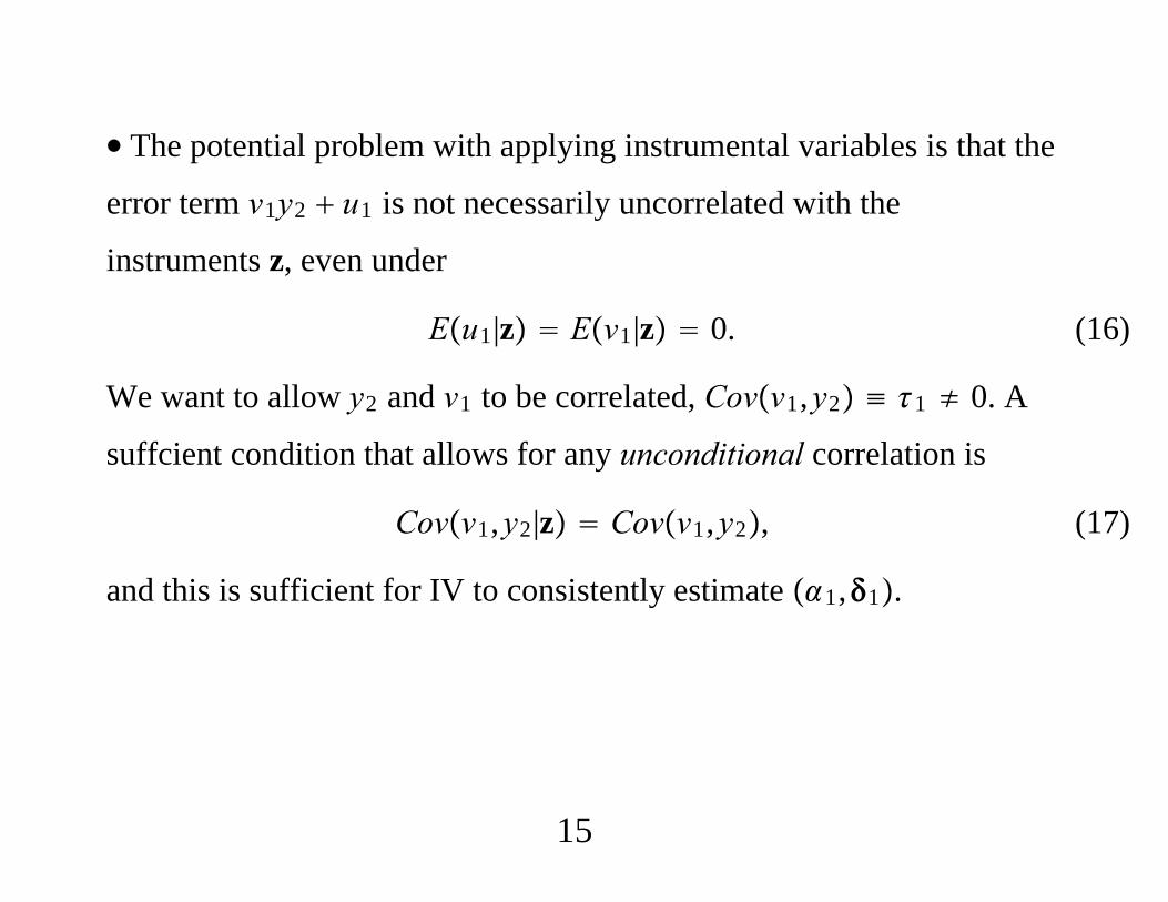
∙ The potential problem with applying instrumental variables is that the

error term v1y2 u1 is not necessarily uncorrelated with the

instruments z, even under

Eu1|z Ev1|z 0. (16)

We want to allow y2 and v1 to be correlated, Covv1,y2 ≡ 1 ≠ 0. A

suffcient condition that allows for any unconditional correlation is

Covv1,y2|z Covv1,y2, (17)

and this is sufficient for IV to consistently estimate 1,1.

15

∙ The usual IV estimator that ignores the randomness in a1 is more

robust than Garen’s (1984) CF estimator, which adds v2 and v2y2 to the

original model, or the Heckman-Vytlacil (1998) “plug-in” estimator,

which replaces y2 with ŷ2 z2.

∙ The condition Covv1,y2|z Covv1,y2 cannot really hold for

discrete y2. Further, Card (2001) shows how it can be violated even if

y2 is continuous. Wooldridge (2005) shows how to allow parametric

heteroskedasticity.

16

∙ In the case of binary y2, we have what is often called the “switching

regression” model. If y2 1z2 v2 ≥ 0 and v2|z Normal0, 1,

then

Ey1|z,y2 1 z11 1y2

1h2y2,z2 1h2y2,z2y2,

where

h2y2,z2 y2z2 − 1 − y2−z2

is the generalized residual function.

17

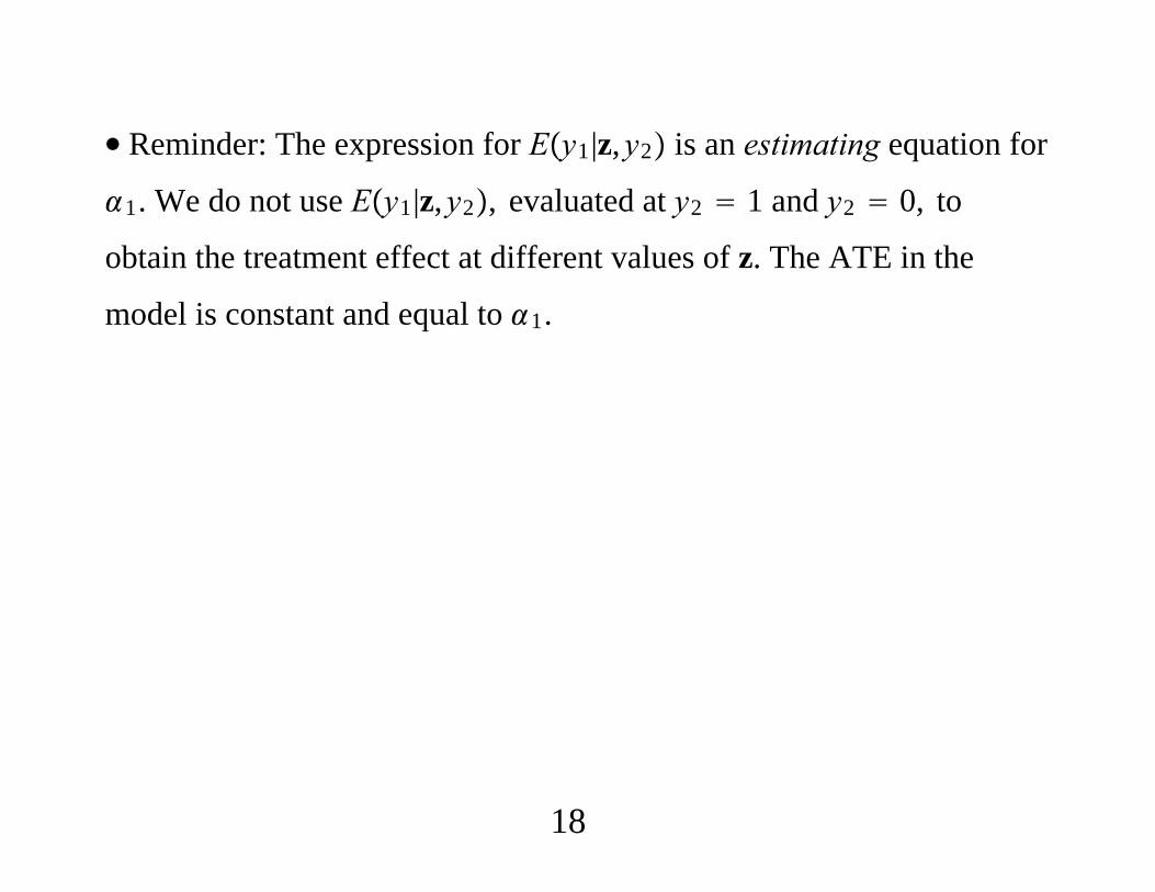
∙ Reminder: The expression for Ey1|z,y2 is an estimating equation for

1. We do not use Ey1|z,y2, evaluated at y2 1 and y2 0, to

obtain the treatment effect at different values of z. The ATE in the

model is constant and equal to 1.

18

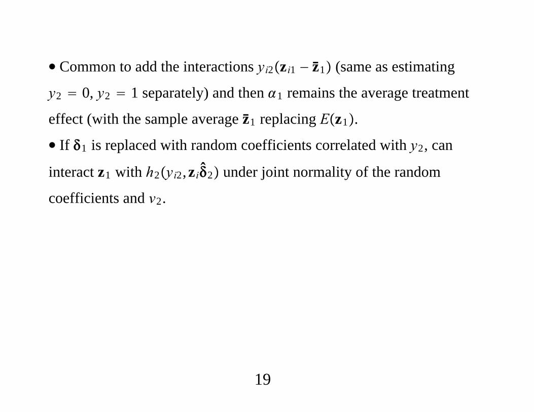
∙ Common to add the interactions yi2zi1 − z1 (same as estimating

y2 0, y2 1 separately) and then 1 remains the average treatment

effect (with the sample average z1 replacing Ez1.

∙ If 1 is replaced with random coefficients correlated with y2, can

interact z1 with h2yi2,zi2 under joint normality of the random

coefficients and v2.

19

∙ Can allow Ev1|v2 to be more flexible [Heckman and MaCurdy

(1986), Powell, Newey, and Walker (1990)].

∙ Also easy to allow for y2 to follow a “heteroskedastic probit” model:

replace v2 with e2 v2/ expz22 where expz22 sde2|z.

Estimate 2, 2 by heteroskedastic probit.

20

3. Nonlinear Models

∙ Typically three approaches to nonlinear models with EEVs.

(1) Plug in fitted values from a first step regression (in an attempt to

mimic 2SLS in linear model). More generally, try to find Ey1|z or

Dy1|z and then impose identifying restrictions.

(2) CF approach: plug in residuals in an attempt to obtain Ey1|y2,z or

Dy1|y2,z.

(3) Maximum Likelihood (often limited information): Use models for

Dy1|y2,z and Dy2|z jointly.

∙ All strategies are more difficult with nonlinear models when y2 is

discrete. Some poor practices have lingered.

21

Binary and Fractional Responses

Probit model:

y1 1z11 1y2 u1 ≥ 0, (18)

where u1|z ~Normal0, 1. Analysis goes through if we replace z1,y2

with any known function x1 ≡ g1z1,y2.

∙ The Rivers-Vuong (1988) approach [Smith and Blundell (1986) for

Tobit] is to make a homoskedastic-normal assumption on the reduced

form for y2,

y2 z2 v2, v2|z Normal0,22. (19)

22

∙ RV approach comes close to requiring

u1,v2 independent of z. (20)

If we also assume

u1,v2 Bivariate Normal (21)

with 1 Corru1,v2, then we can proceed with MLE based on

fy1,y2|z. A CF approach is available, too, based on

Py1 1|z,y2 z11 1y2 1v2 (22)

where each coefficient is multiplied by 1 − 12−1/2.

23

The RV two-step approach is

(i) OLS of y2 on z, to obtain the residuals, v2.

(ii) Probit of y1 on z1,y2, v2 to estimate the scaled coefficients. A

simple t test on v2 is valid to test H0 : 1 0.

∙ Can recover the original coefficients, which appear in the partial

effects. Or,

ASFz1,y2 N−1∑i1

N

x11 1vi2, (23)

that is, we average out the reduced form residuals, vi2. This formulation

is useful for more complicated models.

24

∙ The two-step CF approach easily extends to fractional responses:

Ey1|z,y2,q1 x11 q1, (24)

where x1 is a function of z1,y2 and q1 contains unobservables. Can

use the the same two-step because the Bernoulli log likelihood is in the

linear exponential family. Still estimate scaled coefficients. APEs must

be obtained from (23). To account for first-stage estimation, the

bootstrap is convenient.

∙Wooldridge (2005, Rothenberg Festschrift) describes some simple

ways to make the analysis starting from (24) more flexible, including

allowing Varq1|v2 to be heteroskedastic.

25

Example: Effects of school spending on student performance.. sum math4 lunch rexpp found if y97

Variable | Obs Mean Std. Dev. Min Max---------------------------------------------------------------------

math4 | 1763 .6058803 .1966755 .029 1lunch | 2270 .3614616 .2535764 .0019 .9939rexpp | 2329 4261.201 789.124 1895 11779found | 2357 5895.984 1016.795 4816 10762

. glm math4 lrexpp lunch lenrol lrexpp94 if y97, fam(bin) link(probit) robustnote: math4 has noninteger values

Generalized linear models No. of obs 1208Optimization : ML Residual df 1203

Scale parameter 1

AIC .9079682Log pseudolikelihood -543.4128012 BIC -8378.243

------------------------------------------------------------------------------| Robust

math4 | Coef. Std. Err. z P|z| [95% Conf. Interval]-----------------------------------------------------------------------------

lrexpp | .2726134 .113923 2.39 0.017 .0493285 .4958983lunch | -1.120498 .0582561 -19.23 0.000 -1.234678 -1.006318

lenrol | .0108851 .0390534 0.28 0.780 -.0656581 .0874283lrexpp94 | .1854712 .0829582 2.24 0.025 .0228761 .3480664

_cons | -3.118799 .9207049 -3.39 0.001 -4.923347 -1.31425------------------------------------------------------------------------------

26

. margeff

Average partial effects after glmy Pr(math4)

------------------------------------------------------------------------------variable | Coef. Std. Err. z P|z| [95% Conf. Interval]

-----------------------------------------------------------------------------lrexpp | .0998487 .0416701 2.40 0.017 .0181768 .1815205

lunch | -.4103988 .020199 -20.32 0.000 -.4499882 -.3708094lenrol | .0039868 .0143069 0.28 0.781 -.0240542 .0320278

lrexpp94 | .0679316 .0303795 2.24 0.025 .0083889 .1274742------------------------------------------------------------------------------

. * Compare with OLS:

. reg math4 lrexpp lunch lenrol lrexpp94 if y97, robust

Linear regression Number of obs 1208F( 4, 1203) 106.45Prob F 0.0000R-squared 0.3114Root MSE .168

------------------------------------------------------------------------------| Robust

math4 | Coef. Std. Err. t P|t| [95% Conf. Interval]-----------------------------------------------------------------------------

lrexpp | .0934219 .0415276 2.25 0.025 .0119474 .1748964lunch | -.4205896 .0215956 -19.48 0.000 -.4629588 -.3782204

lenrol | -.0002997 .0146181 -0.02 0.984 -.0289795 .0283802lrexpp94 | .0590509 .0302958 1.95 0.052 -.0003877 .1184894

_cons | -.4838692 .3261972 -1.48 0.138 -1.123848 .1561094------------------------------------------------------------------------------

27

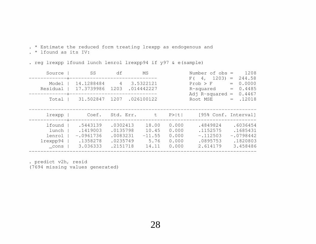
. * Estimate the reduced form treating lrexpp as endogenous and

. * lfound as its IV:

. reg lrexpp lfound lunch lenrol lrexpp94 if y97 & e(sample)

Source | SS df MS Number of obs 1208------------------------------------------- F( 4, 1203) 244.58

Model | 14.1288484 4 3.5322121 Prob F 0.0000Residual | 17.3739986 1203 .014442227 R-squared 0.4485

------------------------------------------- Adj R-squared 0.4467Total | 31.502847 1207 .026100122 Root MSE .12018

------------------------------------------------------------------------------lrexpp | Coef. Std. Err. t P|t| [95% Conf. Interval]

-----------------------------------------------------------------------------lfound | .5443139 .0302413 18.00 0.000 .4849824 .6036454

lunch | .1419003 .0135798 10.45 0.000 .1152575 .1685431lenrol | -.0961736 .0083231 -11.55 0.000 -.112503 -.0798442

lrexpp94 | .1358278 .0235749 5.76 0.000 .0895753 .1820803_cons | 3.036333 .2151718 14.11 0.000 2.614179 3.458486

------------------------------------------------------------------------------

. predict v2h, resid(7694 missing values generated)

28

. glm math4 lrexpp lunch lenrol lrexpp94 v2h if y97, fam(bin) link(probit) robustnote: math4 has noninteger values


Scale parameter 1Deviance 157.5338068 (1/df) Deviance .1310597Pearson 146.5468582 (1/df) Pearson .1219192

Variance function: V(u) u*(1-u/1) [Binomial]Link function : g(u) invnorm(u) [Probit]

AIC .9083169Log pseudolikelihood -542.6234317 BIC -8372.725

------------------------------------------------------------------------------| Robust

math4 | Coef. Std. Err. z P|z| [95% Conf. Interval]-----------------------------------------------------------------------------

lrexpp | .9567996 .2012636 4.75 0.000 .5623302 1.351269lunch | -1.18315 .0585657 -20.20 0.000 -1.297937 -1.068363

lenrol | .0616713 .0399644 1.54 0.123 -.0166574 .14lrexpp94 | -.0784249 .1063432 -0.74 0.461 -.2868536 .1300039

v2h | -.8593559 .2374808 -3.62 0.000 -1.32481 -.3939021_cons | -6.966712 1.259552 -5.53 0.000 -9.435388 -4.498036

------------------------------------------------------------------------------

. * Easily reject null that spending is exogenous.

29

. margeff



-----------------------------------------------------------------------------lrexpp | .3501127 .0734569 4.77 0.000 .2061399 .4940855

lunch | -.432939 .0202452 -21.38 0.000 -.4726189 -.393259lenrol | .0225668 .014639 1.54 0.123 -.0061252 .0512588

lrexpp94 | -.0286973 .0389071 -0.74 0.461 -.1049537 .0475592v2h | -.314455 .086817 -3.62 0.000 -.4846132 -.1442968

------------------------------------------------------------------------------

. * Standard errors need to be fixed up for two-step estimation.

30

. ivreg math4 lunch lenrol lrexpp94 (lrexpp lfound) if y97, robust

Instrumental variables (2SLS) regression Number of obs 1208F( 4, 1203) 114.28Prob F 0.0000R-squared 0.2908Root MSE .1705

------------------------------------------------------------------------------| Robust

math4 | Coef. Std. Err. t P|t| [95% Conf. Interval]-----------------------------------------------------------------------------

lrexpp | .3082997 .0710983 4.34 0.000 .1688093 .4477901lunch | -.4389034 .0219076 -20.03 0.000 -.4818848 -.3959221

lenrol | .0155435 .0154313 1.01 0.314 -.0147317 .0458187lrexpp94 | -.026911 .0393419 -0.68 0.494 -.1040974 .0502754

_cons | -1.66758 .4360251 -3.82 0.000 -2.523035 -.8121261------------------------------------------------------------------------------Instrumented: lrexppInstruments: lunch lenrol lrexpp94 lfound------------------------------------------------------------------------------

31

∙ The control function approach has some decided advantages over

another two-step approach – one that appears to mimic the 2SLS

estimation of the linear model.

∙ Consider the binary response case. Rather than conditioning on v2

along with z (and therefore y2) to obtain

Py1 1|z,v2 Py1 1|z,y2,v2, we can obtain Py1 1|z.

32

∙ To find Py1 1|z, we plug in the reduced form for y2 to get

y1 1z11 1z2 1v2 u1 0. Because 1v2 u1 is

independent of z and normally distributed,

Py1 1|z z11 1z2/1. So first do OLS on the reduced

form, and get fitted values, ŷi2 zi2. Then, probit of yi1 on zi1,ŷi2 to

estimate scaled coefficients. Harder to estimate APEs and test for

endogeneity.

33

∙ Danger with plugging in fitted values for y2 is that one might be

tempted to plug ŷ2 into nonlinear functions, say y22 or y2z1. This does

not result in consistent estimation of the scaled parameters or the

partial effects. If we believe y2 has a linear RF with additive normal

error independent of z, the addition of v2 solves the endogeneity

problem regardless of how y2 appears. Plugging in fitted values for y2

only works in the case where the model is linear in y2. Plus, the CF

approach makes it much easier to test the null that for endogeneity of y2

as well as compute APEs.

34

∙ Can understand the limits of CF approach by returning to

Ey1|z,y2,q1 z11 1y2 q1, where y2 is discrete.

Rivers-Vuong approach does not generally work.

∙ Suppose y1 and y2 are both binary and

y2 1z2 v2 ≥ 0 (25)

and we maintain joint normality of u1,v2. We should not try to mimic

2SLS as follows: (i) Do probit of y2 on z and get the fitted probabilities,

2 z2. (ii) Do probit of y1 on z1, 2, that is, just replace y2 with

2.

35

∙ In general, the only strategy we have is maximum likelihood

estimation based on fy1|y2,zfy2|z. [Perhaps this is why some, such

as Angrist (2001), Angrist and Pischke (2009), promote the notion of

just using linear probability models estimated by 2SLS.]

∙ “Bivariate probit” software can be used to estimate the probit model

with a binary endogenous variable.

∙ Parallel discussions hold for ordered probit, Tobit.

36

Multinomial Responses

∙ Recent push by Petrin and Train (2006), among others, to use control

function methods where the second step estimation is something simple

– such as multinomial logit, or nested logit – rather than being derived

from a structural model. So, if we have reduced forms

y2 z2 v2, (26)

then we jump directly to convenient models for Py1 j|z1,y2,v2.

The average structural functions are obtained by averaging the response

probabilities across vi2. No convincing way to handle discrete y2,

though.

37

Exponential Models

∙ IV and CF approaches available for exponential models. Write

Ey1|z,y2, r1 expz11 1y2 r1, (27)

where r1 is the omitted variable. As usual, CF methods based on

Ey1|z,y2 expz11 1y2Eexpr1|z,y2.

For continuous y2, can find Ey1|z,y2 when Dy2|z is homoskedastic

normal (Wooldridge, 1997) and when Dy2|z follows a probit (Terza,

1998). In the probit case,

Ey1|z,y2 expz11 1y2hy2,z2,1

38

hy2,z2,1 exp12/2y21 z2/z2

1 − y21 − 1 z2/1 − z2.

∙ IV methods that work for any y2 are available [Mullahy (1997)]. If

Ey1|z,y2, r1 expx11 r1 (28)

and r1 is independent of z then

Eexp−x11y1|z Eexpr1|z 1, (29)

where Eexpr1 1 is a normalization. The moment conditions are

Eexp−x11y1 − 1|z 0. (30)

39

4. Semiparametric and Nonparametric Approaches

∙ Blundell and Powell (2004) show how to relax distributional

assumptions on u1,v2 in the model y1 1x11 u1 0, where x1

can be any function of z1,y2. Their key assumption is that y2 can be

written as y2 g2z v2, where u1,v2 is independent of z, which

rules out discreteness in y2. Then

Py1 1|z,v2 Ey1|z,v2 Hx11,v2 (31)

for some (generally unknown) function H, . The average structural

function is just ASFz1,y2 Evi2Hx11,vi2.

40

∙ Two-step estimation: Estimate the function g2 and then obtain

residuals vi2 yi2 − ĝ2zi. BP (2004) show how to estimate H and 1

(up to scaled) and G, the distribution of u1. The ASF is obtained

from Gx11 or

ASFz1,y2 N−1∑i1

N

Ĥx11, vi2; (32)

∙ Blundell and Powell (2003) allow Py1 1|z,y2 to have general

form Hz1,y2,v2, and the second-step estimation is entirely

nonparametric. Further, ĝ2 can be fully nonparametric. Parametric

approximations might produce good estimates of the APEs.

41

∙ BP (2003) consider a very general setup: y1 g1z1,y2,u1, with

ASF1z1,y2 g1z1,y2,u1dF1u1, (33)

where F1 is the distribution of u1. Key restrictions are that y2 can be

written as

y2 g2z v2, (34)

where u1,v2 is independent of z.

42

∙ Key: ASF can be obtained from Ey1|z1,y2,v2 h1z1,y2,v2 by

averaging out v2, and fully nonparametric two-step estimates are

available.

∙ The focus on the ASF is liberating. It justifies flexible parametric

approaches that need not be tied to “structural” equations. In particular,

we can just skip modeling g1 and start with Ey1|z1,y2,v2.

∙ For example, if y1 is binary or a fraction and y2 is a scalar,

Ey1|z1,y2,v2 z11 1y2 1v2 1v22

z1v21 1y2v2 . . .

43

5. Methods for Panel Data

∙ Combine methods for correlated random effects models with CF

methods for nonlinear panel data models with unobserved

heterogeneity and EEVs.

∙ Illustrate a parametric approach used by Papke and Wooldridge

(2008), which applies to binary and fractional responses.

∙ Nothing appears to be known about applying “fixed effects” probit to

estimate the fixed effects while also dealing with endogeneity. Likely

to be poor for small T.

44

∙Model with time-constant unobserved heterogeneity, ci1, and

time-varying unobservables, vit1, as

Eyit1|yit2,zi,ci1,vit1 1yit2 zit11

ci1 vit1. (35)

Allow the heterogeneity, ci1, to be correlated with yit2 and zi, where

zi zi1, . . . ,ziT is the vector of strictly exogenous variables

(conditional on ci1). The time-varying omitted variable, vit1, is

uncorrelated with zi – strict exogeneity – but may be correlated with

yit2. As an example, yit1 is a female labor force participation indicator

and yit2 is other sources of income.

45

∙Write zit zit1,zit2, so that the time-varying IVs zit2 are excluded

from the “structural.”

∙ Chamberlain approach:

ci1 1 zi1 ai1,ai1|zi ~ Normal0,a12 . (36)

Next step:

Eyit1|yit2,zi, rit1 1yit2 zit11 1 zi1 rit1

where rit1 ai1 vit1. Next, assume a linear reduced form for yit2:

yit2 2 zit2 zi2 vit2, t 1, . . . ,T. (37)

46

∙ Rules out discrete yit2 because

rit1 1vit2 eit1, (38)

eit1|zi,vit2 ~ Normal0,e12 , t 1, . . . ,T. (39)

Then

Eyit1|zi,yit2,vit2 e1yit2 zit1e1 e1 zie1 e1vit2 (40)

where the “e” subscript denotes division by 1 e12 1/2. This equation

is the basis for CF estimation.

47

∙ Simple two-step procedure: (i) Estimate the reduced form for yit2(pooled across t, or maybe for each t separately; at a minimum,

different time period intercepts should be allowed). Obtain the

residuals, vit2 for all i, t pairs. The estimate of 2 is the fixed effects

estimate. (ii) Use the pooled probit (quasi)-MLE of yit1 on

yit2,zit1, zi, vit2 to estimate e1,e1,e1,e1 and e1.

∙ Delta method or bootstrapping (resampling cross section units) for

standard errors. Can ignore first-stage estimation to test e1 0 (but

test should be fully robust to variance misspecification and serial

independence).

48

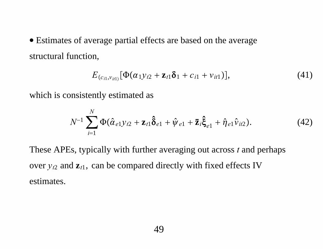
∙ Estimates of average partial effects are based on the average

structural function,

Eci1,vit1 1yt2 zt11 ci1 vit1, (41)

which is consistently estimated as

N−1∑i1

N

e1yt2 zt1e1 e1 zie1 e1vit2. (42)

These APEs, typically with further averaging out across t and perhaps

over yt2 and zt1, can be compared directly with fixed effects IV

estimates.

49

EXAMPLE: Effects of Spending on Test Pass Rates

∙ Reform occurs between 1993/94 and 1994/95 school year; its passage

was a surprise to almost everyone.

∙ Since 1994/95, each district receives a foundation allowance, based

on revenues in 1993/94.

∙ Intially, all districts were brought up to a minimum allowance –

$4,200 in the first year. The goal was to eventually give each district a

basic allowance ($5,000 in the first year).

∙ Districts divided into three groups in 1994/95 for purposes of initial

foundation allowance. Subsequent grants determined by statewide

School Aid Fund.

50

∙ Catch-up formula for districts receiving below the basic. Initially,

more than half of the districts received less than the basic allowance.

By 1998/99, it was down to about 36%. In 1999/00, all districts began

receiving the basic allowance, which was then $5,700. Two-thirds of all

districts now receive the basic allowance.

∙ From 1991/92 to 2003/04, in the 10th percentile, expenditures rose

from $4,616 (2004 dollars) to $7,125, a 54 percent increase. In the 50th

percentile, it was a 48 percent increase. In the 90th percentile, per pupil

expenditures rose from $7,132 in 1992/93 to $9,529, a 34 percent

increase.

51

∙ Response variable: math4, the fraction of fourth graders passing the

MEAP math test at a school.

∙ Spending variable is logavgrexppp, where the average is over the

current and previous three years.

∙ The linear model is

math4it t 1 logavgrexpit 2lunchit 3 logenrollit ci1 uit1

Estimating this model by fixed effects is identical to adding the time

averages of the three explanatory variables and using pooled OLS.

∙ The “fractional probit” model:

Emath4it|xi1,xi2, . . . ,xiT at xita xia.

52

∙ Allowing spending to be endogenous. Controlling for 1993/94

spending, foundation grant should be exogenous. Exploit

nonsmoothness in the grant as a function of initial spending.

math4it t 1 logavgrexpit 2lunchit 3 logenrollit

4t logrexpppi,1994 1lunchi 2logenrolli vit1

∙ And, fractional probit version of this.

53

. use meap92_01

. xtset distid yearpanel variable: distid (strongly balanced)

time variable: year, 1992 to 2001delta: 1 unit

. des math4 avgrexp lunch enroll found

storage display valuevariable name type format label variable label-------------------------------------------------------------------------------math4 double %9.0g fraction satisfactory, 4th

grade mathavgrexp float %9.0g (rexppp rexppp_1 rexppp_2

rexppp_3)/4lunch float %9.0g fraction eligible for free lunchenroll float %9.0g district enrollmentfound int %9.0g foundation grant, $: 1995-2001

. sum math4 rexppp lunch

Variable | Obs Mean Std. Dev. Min Max---------------------------------------------------------------------

math4 | 5010 .6149834 .1912023 .059 1rexppp | 5010 6331.99 1168.198 3553.361 15191.49

lunch | 5010 .2802852 .1571325 .0087 .9126999

54

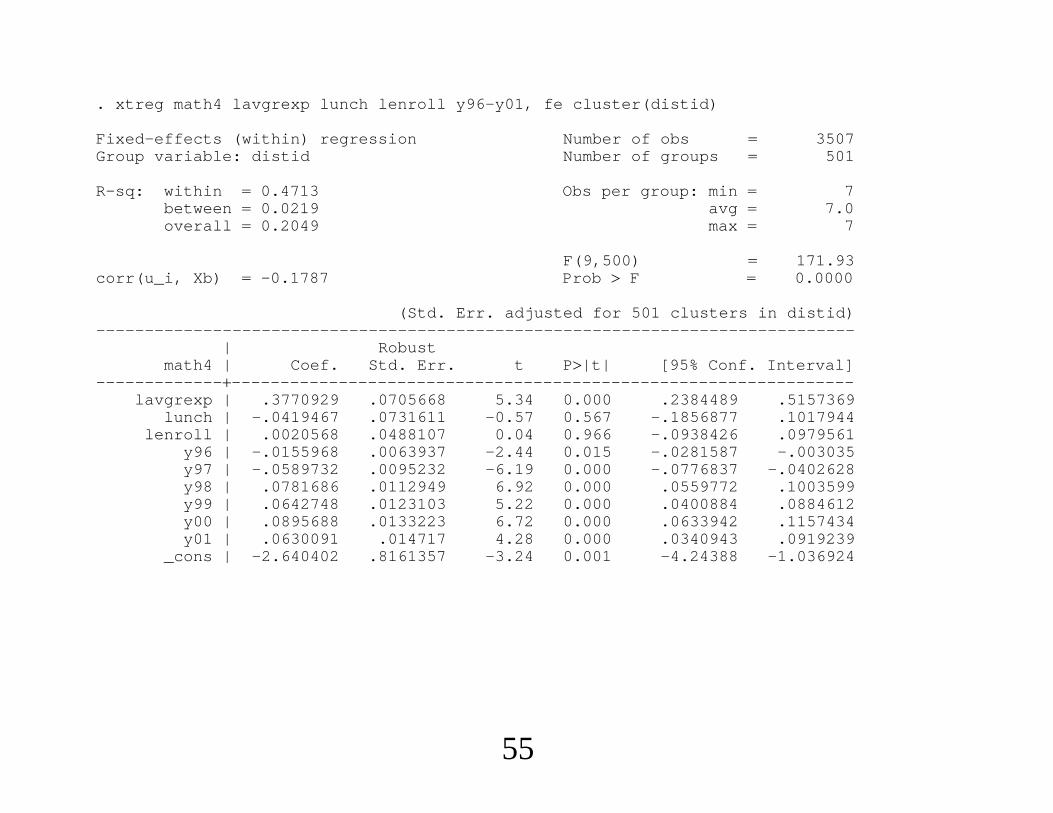
. xtreg math4 lavgrexp lunch lenroll y96-y01, fe cluster(distid)

Fixed-effects (within) regression Number of obs 3507Group variable: distid Number of groups 501

R-sq: within 0.4713 Obs per group: min 7between 0.0219 avg 7.0overall 0.2049 max 7

F(9,500) 171.93corr(u_i, Xb) -0.1787 Prob F 0.0000

(Std. Err. adjusted for 501 clusters in distid)------------------------------------------------------------------------------

| Robustmath4 | Coef. Std. Err. t P|t| [95% Conf. Interval]

-----------------------------------------------------------------------------lavgrexp | .3770929 .0705668 5.34 0.000 .2384489 .5157369

lunch | -.0419467 .0731611 -0.57 0.567 -.1856877 .1017944lenroll | .0020568 .0488107 0.04 0.966 -.0938426 .0979561

y96 | -.0155968 .0063937 -2.44 0.015 -.0281587 -.003035y97 | -.0589732 .0095232 -6.19 0.000 -.0776837 -.0402628y98 | .0781686 .0112949 6.92 0.000 .0559772 .1003599y99 | .0642748 .0123103 5.22 0.000 .0400884 .0884612y00 | .0895688 .0133223 6.72 0.000 .0633942 .1157434y01 | .0630091 .014717 4.28 0.000 .0340943 .0919239

_cons | -2.640402 .8161357 -3.24 0.001 -4.24388 -1.036924

55

-----------------------------------------------------------------------------sigma_u | .1130256sigma_e | .08314135

rho | .64888558 (fraction of variance due to u_i)------------------------------------------------------------------------------

. des alavgrexp alunch alenroll

storage display valuevariable name type format label variable label-------------------------------------------------------------------------------alavgrexp float %9.0g time average lavgrexp, 1995-2001alunch float %9.0g time average lunch, 1995-2001alenroll float %9.0g time average lenroll, 1995-2001

56

. reg math4 lavgrexp alavgrexp lunch alunch lenroll alenroll y96-y01,cluster(distid)




-----------------------------------------------------------------------------lavgrexp | .377092 .0705971 5.34 0.000 .2383884 .5157956

alavgrexp | -.286541 .0731797 -3.92 0.000 -.4303185 -.1427635lunch | -.0419466 .0731925 -0.57 0.567 -.1857494 .1018562

alunch | -.3770088 .0766141 -4.92 0.000 -.5275341 -.2264835lenroll | .0020566 .0488317 0.04 0.966 -.093884 .0979972

alenroll | -.0031646 .0491534 -0.06 0.949 -.0997373 .0934082y96 | -.0155968 .0063965 -2.44 0.015 -.0281641 -.0030295y97 | -.0589731 .0095273 -6.19 0.000 -.0776916 -.0402546y98 | .0781687 .0112998 6.92 0.000 .0559678 .1003696y99 | .064275 .0123156 5.22 0.000 .0400782 .0884717y00 | .089569 .013328 6.72 0.000 .0633831 .1157548y01 | .0630093 .0147233 4.28 0.000 .0340821 .0919365

_cons | -.0006233 .2450239 -0.00 0.998 -.4820268 .4807801------------------------------------------------------------------------------

57

. * Now use fractional probit.

. glm math4 lavgrexp alavgrexp lunch alunch lenroll alenroll y96-y01,fa(bin) link(probit) cluster(distid)

note: math4 has non-integer values




| Robustmath4 | Coef. Std. Err. z P|z| [95% Conf. Interval]

-----------------------------------------------------------------------------lavgrexp | .8810302 .2068026 4.26 0.000 .4757045 1.286356

alavgrexp | -.5814474 .2229411 -2.61 0.009 -1.018404 -.1444909lunch | -.2189714 .2071544 -1.06 0.290 -.6249865 .1870437

alunch | -.9966635 .2155739 -4.62 0.000 -1.419181 -.5741465lenroll | .0887804 .1382077 0.64 0.521 -.1821017 .3596626

alenroll | -.0893612 .1387674 -0.64 0.520 -.3613404 .1826181y96 | -.0362309 .0178481 -2.03 0.042 -.0712125 -.0012493y97 | -.1467327 .0273205 -5.37 0.000 -.20028 -.0931855y98 | .2520084 .0337706 7.46 0.000 .1858192 .3181975y99 | .2152507 .0367226 5.86 0.000 .1432757 .2872257y00 | .3049632 .0399409 7.64 0.000 .2266805 .3832459y01 | .2257321 .0439608 5.13 0.000 .1395705 .3118938

_cons | -1.855832 .7556621 -2.46 0.014 -3.336902 -.3747616------------------------------------------------------------------------------

58

. margeff



-----------------------------------------------------------------------------lavgrexp | .2968496 .0695326 4.27 0.000 .1605682 .433131

alavgrexp | -.1959097 .0750686 -2.61 0.009 -.3430414 -.0487781lunch | -.0737791 .0698318 -1.06 0.291 -.2106469 .0630887

alunch | -.3358104 .0723725 -4.64 0.000 -.4776579 -.1939629lenroll | .0299132 .0465622 0.64 0.521 -.061347 .1211734

alenroll | -.0301089 .0467477 -0.64 0.520 -.1217326 .0615149y96 | -.0122924 .0061107 -2.01 0.044 -.0242692 -.0003156y97 | -.0508008 .0097646 -5.20 0.000 -.069939 -.0316625y98 | .0809879 .0100272 8.08 0.000 .0613349 .1006408y99 | .0696954 .0111375 6.26 0.000 .0478662 .0915245y00 | .0970224 .0115066 8.43 0.000 .0744698 .119575y01 | .0729829 .0132849 5.49 0.000 .046945 .0990208

------------------------------------------------------------------------------

. * These standard errors are very close to bootstrapped standard errors.

59

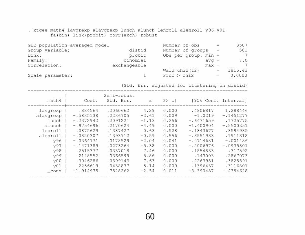
. xtgee math4 lavgrexp alavgrexp lunch alunch lenroll alenroll y96-y01,fa(bin) link(probit) corr(exch) robust

GEE population-averaged model Number of obs 3507Group variable: distid Number of groups 501Link: probit Obs per group: min 7Family: binomial avg 7.0Correlation: exchangeable max 7

Wald chi2(12) 1815.43Scale parameter: 1 Prob chi2 0.0000

(Std. Err. adjusted for clustering on distid)------------------------------------------------------------------------------

| Semi-robustmath4 | Coef. Std. Err. z P|z| [95% Conf. Interval]

-----------------------------------------------------------------------------lavgrexp | .884564 .2060662 4.29 0.000 .4806817 1.288446

alavgrexp | -.5835138 .2236705 -2.61 0.009 -1.0219 -.1451277lunch | -.2372942 .2091221 -1.13 0.256 -.6471659 .1725775

alunch | -.9754696 .2170624 -4.49 0.000 -1.400904 -.5500351lenroll | .0875629 .1387427 0.63 0.528 -.1843677 .3594935

alenroll | -.0820307 .1393712 -0.59 0.556 -.3551933 .1911318y96 | -.0364771 .0178529 -2.04 0.041 -.0714681 -.001486y97 | -.1471389 .0273264 -5.38 0.000 -.2006976 -.0935801y98 | .2515377 .0337018 7.46 0.000 .1854833 .317592y99 | .2148552 .0366599 5.86 0.000 .143003 .2867073y00 | .3046286 .0399143 7.63 0.000 .2263981 .3828591y01 | .2256619 .0438877 5.14 0.000 .1396437 .3116801

_cons | -1.914975 .7528262 -2.54 0.011 -3.390487 -.4394628------------------------------------------------------------------------------

60

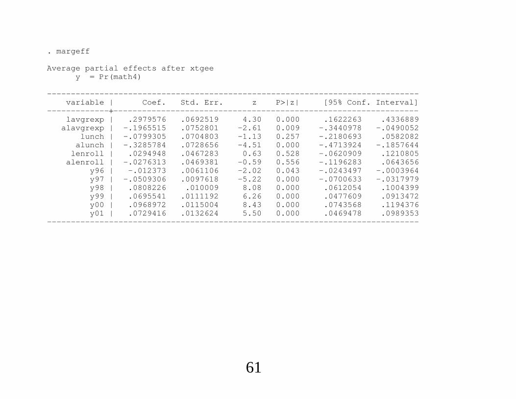
. margeff

Average partial effects after xtgeey Pr(math4)


-----------------------------------------------------------------------------lavgrexp | .2979576 .0692519 4.30 0.000 .1622263 .4336889

alavgrexp | -.1965515 .0752801 -2.61 0.009 -.3440978 -.0490052lunch | -.0799305 .0704803 -1.13 0.257 -.2180693 .0582082

alunch | -.3285784 .0728656 -4.51 0.000 -.4713924 -.1857644lenroll | .0294948 .0467283 0.63 0.528 -.0620909 .1210805

alenroll | -.0276313 .0469381 -0.59 0.556 -.1196283 .0643656y96 | -.012373 .0061106 -2.02 0.043 -.0243497 -.0003964y97 | -.0509306 .0097618 -5.22 0.000 -.0700633 -.0317979y98 | .0808226 .010009 8.08 0.000 .0612054 .1004399y99 | .0695541 .0111192 6.26 0.000 .0477609 .0913472y00 | .0968972 .0115004 8.43 0.000 .0743568 .1194376y01 | .0729416 .0132624 5.50 0.000 .0469478 .0989353

------------------------------------------------------------------------------

61

. * Now allow spending to be endogenous. Use foundation allowance, and

. * interactions, as IVs.

. * First, linear model:

. ivreg math4 lunch alunch lenroll alenroll y96-y01 lexppp94 le94y96-le94y01(lavgrexp lfound lfndy96-lfndy01), cluster(distid)

Instrumental variables (2SLS) regression Number of obs 3507F( 18, 500) 107.05Prob F 0.0000R-squared 0.4134Root MSE .11635



-----------------------------------------------------------------------------lavgrexp | .5545247 .2205466 2.51 0.012 .1212123 .987837

lunch | -.0621991 .0742948 -0.84 0.403 -.2081675 .0837693alunch | -.4207815 .0758344 -5.55 0.000 -.5697749 -.2717882

lenroll | .0463616 .0696215 0.67 0.506 -.0904253 .1831484alenroll | -.049052 .070249 -0.70 0.485 -.1870716 .0889676

y96 | -1.085453 .2736479 -3.97 0.000 -1.623095 -.5478119y97 | -1.049922 .376541 -2.79 0.005 -1.78972 -.3101244y98 | -.4548311 .4958826 -0.92 0.359 -1.429102 .5194394y99 | -.4360973 .5893671 -0.74 0.460 -1.594038 .7218439y00 | -.3559283 .6509999 -0.55 0.585 -1.634961 .923104y01 | -.704579 .7310773 -0.96 0.336 -2.140941 .7317831

lexppp94 | -.4343213 .2189488 -1.98 0.048 -.8644944 -.0041482le94y96 | .1253255 .0318181 3.94 0.000 .0628119 .1878392le94y97 | .11487 .0425422 2.70 0.007 .0312865 .1984534le94y98 | .0599439 .0554377 1.08 0.280 -.0489757 .1688636le94y99 | .0557854 .0661784 0.84 0.400 -.0742367 .1858075le94y00 | .048899 .0727172 0.67 0.502 -.0939699 .1917678

62

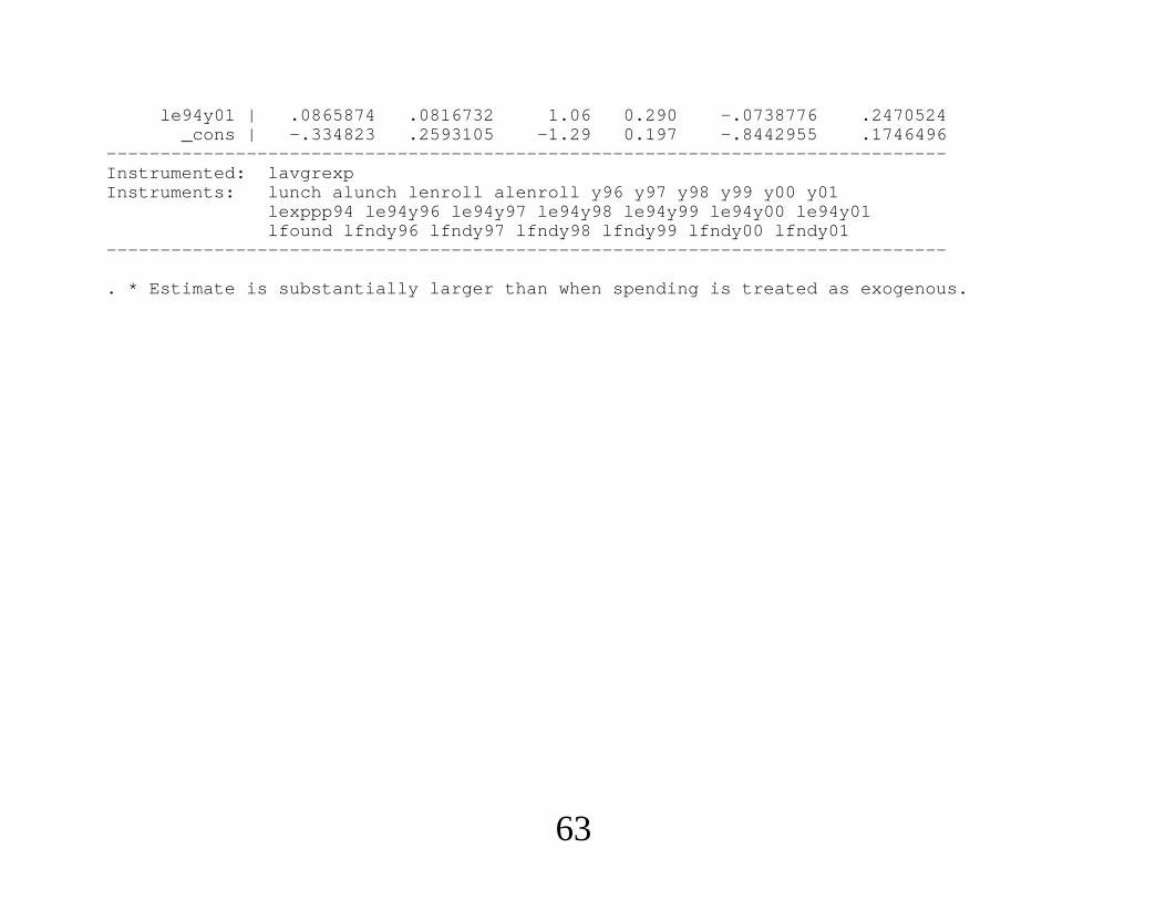
le94y01 | .0865874 .0816732 1.06 0.290 -.0738776 .2470524_cons | -.334823 .2593105 -1.29 0.197 -.8442955 .1746496

------------------------------------------------------------------------------Instrumented: lavgrexpInstruments: lunch alunch lenroll alenroll y96 y97 y98 y99 y00 y01

lexppp94 le94y96 le94y97 le94y98 le94y99 le94y00 le94y01lfound lfndy96 lfndy97 lfndy98 lfndy99 lfndy00 lfndy01

------------------------------------------------------------------------------

. * Estimate is substantially larger than when spending is treated as exogenous.

63

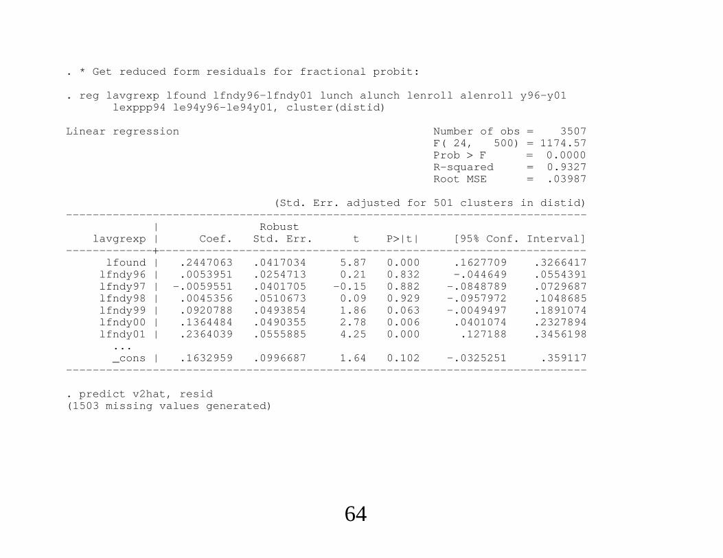
. * Get reduced form residuals for fractional probit:

. reg lavgrexp lfound lfndy96-lfndy01 lunch alunch lenroll alenroll y96-y01lexppp94 le94y96-le94y01, cluster(distid)



| Robustlavgrexp | Coef. Std. Err. t P|t| [95% Conf. Interval]

-----------------------------------------------------------------------------lfound | .2447063 .0417034 5.87 0.000 .1627709 .3266417

lfndy96 | .0053951 .0254713 0.21 0.832 -.044649 .0554391lfndy97 | -.0059551 .0401705 -0.15 0.882 -.0848789 .0729687lfndy98 | .0045356 .0510673 0.09 0.929 -.0957972 .1048685lfndy99 | .0920788 .0493854 1.86 0.063 -.0049497 .1891074lfndy00 | .1364484 .0490355 2.78 0.006 .0401074 .2327894lfndy01 | .2364039 .0555885 4.25 0.000 .127188 .3456198

..._cons | .1632959 .0996687 1.64 0.102 -.0325251 .359117

------------------------------------------------------------------------------

. predict v2hat, resid(1503 missing values generated)

64

. glm math4 lavgrexp v2hat lunch alunch lenroll alenroll y96-y01 lexppp94le94y96-le94y01, fa(bin) link(probit) cluster(distid)

note: math4 has non-integer values



Variance function: V(u) u*(1-u/1) [Binomial]Link function : g(u) invnorm(u) [Probit]


| Robustmath4 | Coef. Std. Err. z P|z| [95% Conf. Interval]

-----------------------------------------------------------------------------lavgrexp | 1.731039 .6541194 2.65 0.008 .4489886 3.013089

v2hat | -1.378126 .720843 -1.91 0.056 -2.790952 .0347007lunch | -.2980214 .2125498 -1.40 0.161 -.7146114 .1185686

alunch | -1.114775 .2188037 -5.09 0.000 -1.543623 -.685928lenroll | .2856761 .197511 1.45 0.148 -.1014383 .6727905

alenroll | -.2909903 .1988745 -1.46 0.143 -.6807771 .0987966...

_cons | -2.455592 .7329693 -3.35 0.001 -3.892185 -1.018998------------------------------------------------------------------------------

65

. margeff



-----------------------------------------------------------------------------lavgrexp | .5830163 .2203345 2.65 0.008 .1511686 1.014864

v2hat | -.4641533 .242971 -1.91 0.056 -.9403678 .0120611lunch | -.1003741 .0716361 -1.40 0.161 -.2407782 .04003

alunch | -.3754579 .0734083 -5.11 0.000 -.5193355 -.2315803lenroll | .0962161 .0665257 1.45 0.148 -.0341719 .2266041

alenroll | -.0980059 .0669786 -1.46 0.143 -.2292817 .0332698...

------------------------------------------------------------------------------

. * These standard errors do not account for the first-stage estimation. Should

. * use the panel bootstrap accounting for both stages.

. * Only marginal evidence that spending is endogenous, but the negative sign

. * fits the story that districts increase spending when performance is

. * (expected to be) worse, based on unobservables (to us).

66

Model: Linear Fractional ProbitEstimation Method: Instrumental Variables Pooled QMLE

Coefficient Coefficient APElog(arexppp) .555 1.731 .583

(.221) (.759) (.255)lunch −. 062 −. 298 −. 100

. 074 (.202) (.068)log(enroll) .046 .286 .096

(.070) (.209) (.070)v2 −. 424 −1. 378 —

(.232) (.811) —Scale Factor — .337

67

control function and related methods jeff wooldridge … · control function and related methods...

Documents