STRATIFIED SAMPLING

Jeff WooldridgeMichigan State UniversityLABOUR Lectures, EIEF

October 18-19, 2011

1. The Basic Methodology2. Regression Models3. Nonlinear Models4. General Treatment of Exogenous Stratification

1

1. The Basic Methodology

∙With stratified sampling, some segments of the population are

overrepresented or underrepresented by the sampling scheme. If we

know enough information about the stratification scheme (and the

population), we can modify standard econometric methods and

consistently estimate population parameters.

∙ There are two common types of stratified sampling, standard

stratified (SS) sampling and variable probability (VP) sampling. A third

type of sampling, typically called multinomial sampling, is practically

indistinguishable from SS sampling, but it generates a random sample

from a modified population.

2

∙ SS Sampling: Partition the sample space, sayW, into G

non-overlapping, exhaustive groups, Wg : g 1, . . .G. A random

sample is taken from each group g, say wgi : i 1, . . . ,Ng, where Ng

is the number of observations drawn from stratum g and

N N1 N2 . . .NG is the total number of observations.

∙ Let w be a random vector representing the population. Each each

random draw from stratum g has the same distribution as w conditional

on w belonging to Wg:

Dwgi Dw|w ∈ Wg, i 1, . . . ,Ng. (1.1)

∙We only know we have an SS sample if we are told.

3

∙What if we want to estimate the mean of w from an SS sample? Let

g Pw ∈Wg be the probability that w falls into stratum g; the g,

which are population frequencies, are often called the “aggregate

shares.” If we know the g (or can consistently estimate them), then

w Ew is identified by a weighted average of the expected values

for the strata:

w 1Ew|w ∈ W1 . . .GEw|w ∈ WG. (1.2)

∙ Sometimes the g are obtained from census data.

4

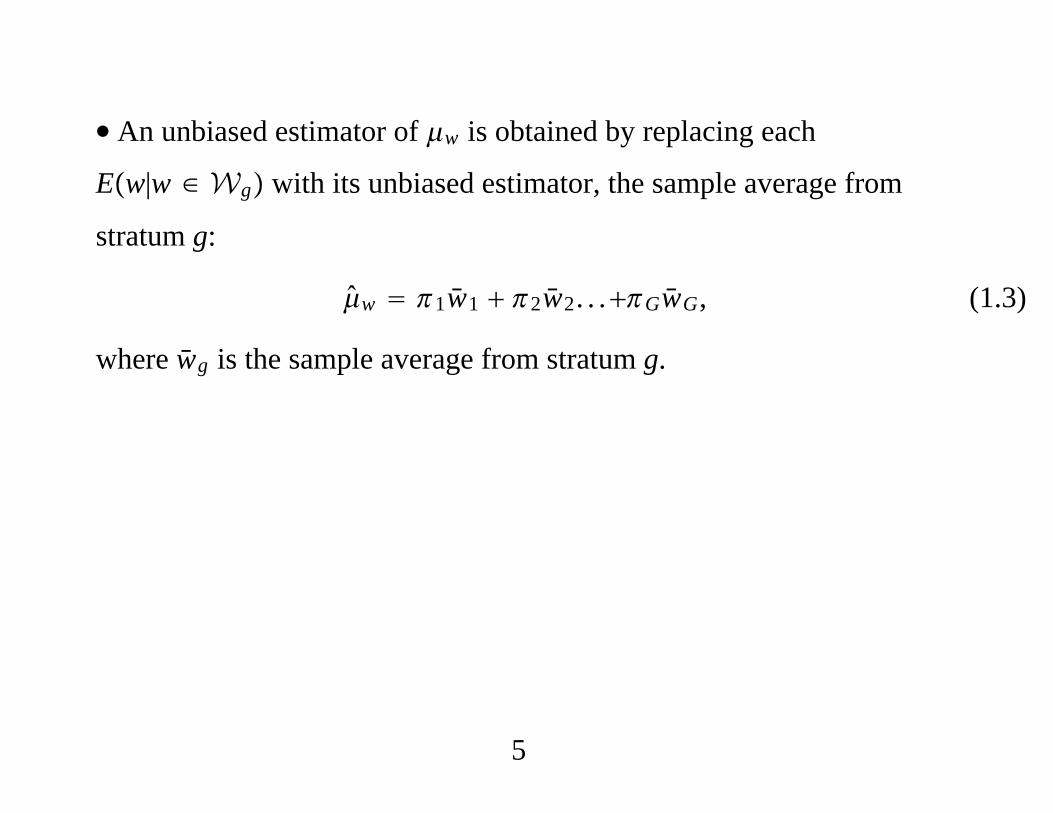
∙ An unbiased estimator of w is obtained by replacing each

Ew|w ∈ Wg with its unbiased estimator, the sample average from

stratum g:

w 1w1 2w2. . .GwG, (1.3)

where wg is the sample average from stratum g.

5

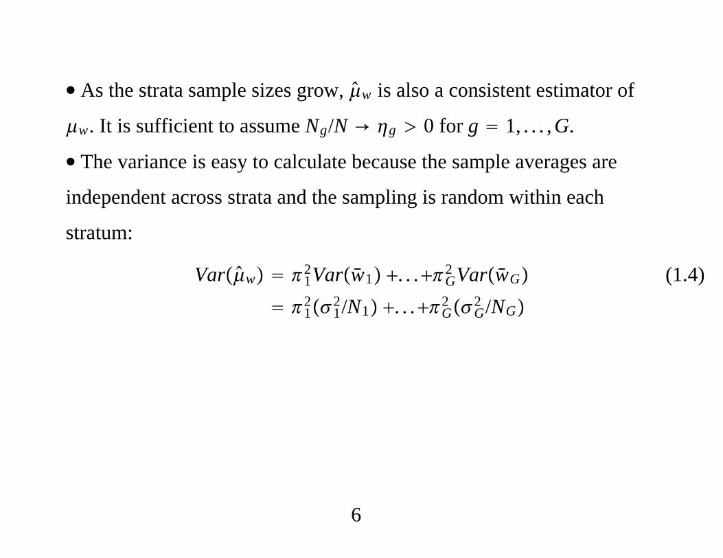
∙ As the strata sample sizes grow, w is also a consistent estimator of

w. It is sufficient to assume Ng/N → g 0 for g 1, . . . ,G.

∙ The variance is easy to calculate because the sample averages are

independent across strata and the sampling is random within each

stratum:

Varw 12Varw1 . . .G

2 VarwG

121

2/N1 . . .G2 G

2 /NG

(1.4)

6

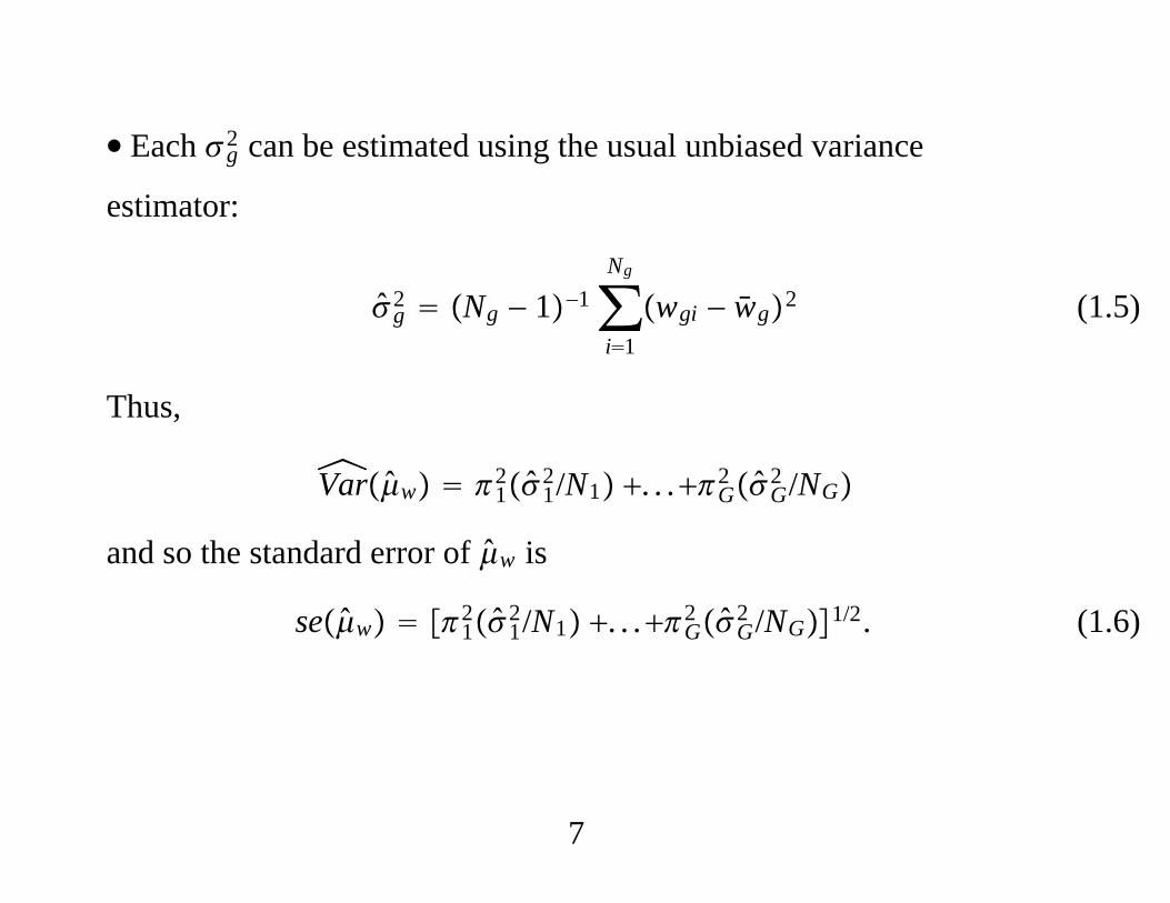
∙ Each g2 can be estimated using the usual unbiased variance

estimator:

g2 Ng − 1−1∑

i1

Ng

wgi − wg2 (1.5)

Thus,

Varw 121

2/N1 . . .G2 G

2 /NG

and so the standard error of w is

sew 121

2/N1 . . .G2 G

2 /NG1/2. (1.6)

7

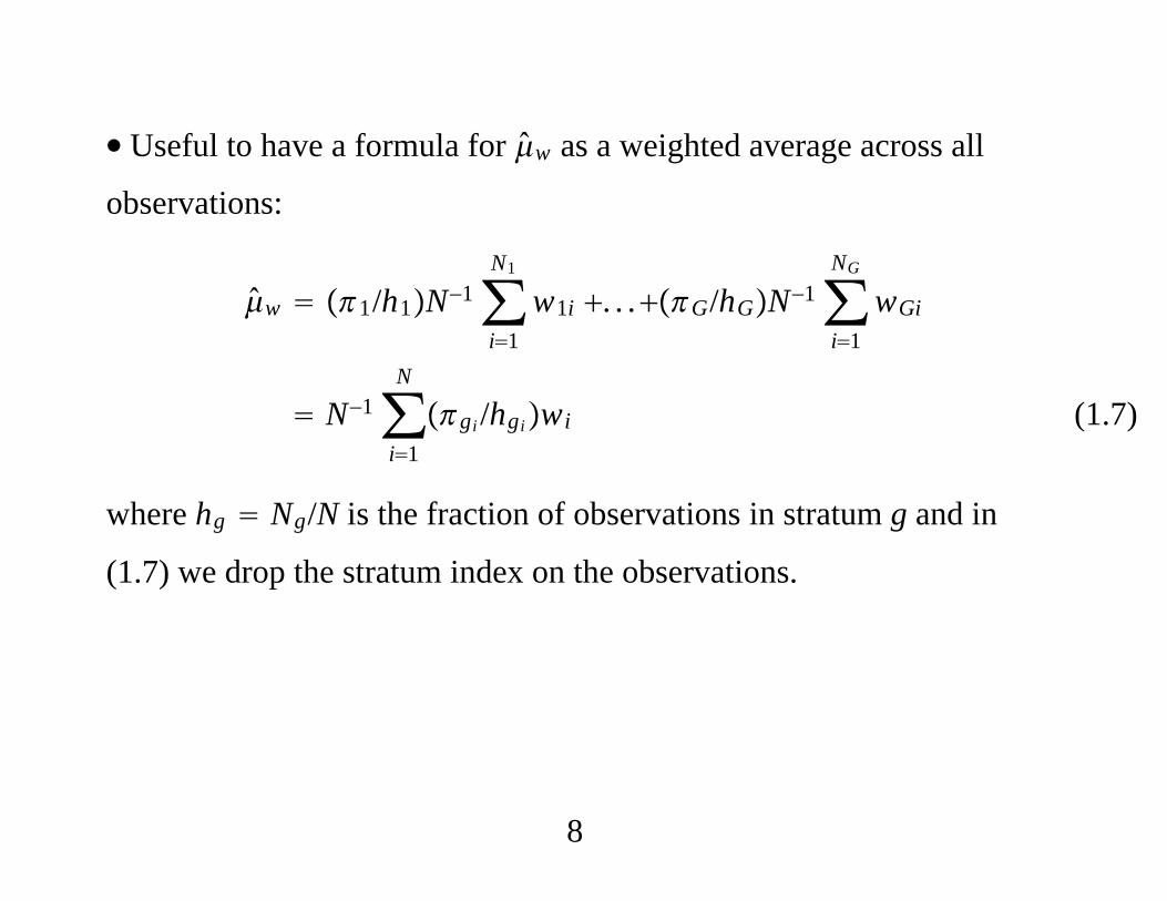
∙ Useful to have a formula for w as a weighted average across all

observations:

w 1/h1N−1∑i1

N1

w1i . . .G/hGN−1∑i1

NG

wGi

N−1∑i1

N

gi /hgiwi (1.7)

where hg Ng/N is the fraction of observations in stratum g and in

(1.7) we drop the stratum index on the observations.

8

∙ Variable Probability Sampling: Often used where little, if anything,

is known about respondents ahead of time. Still partition the sample

space, but a unit is drawn at random from the population. If the

observation falls into stratum g, it is kept with (nonzero) sampling

probability, pg. That is, random draw wi is kept with probability pg if

wi ∈ Wg.

∙ The population is sampled N times (N not always reported with VP

samples). We always know how many data points were kept; call this

M – a random variable. Let si be a selection indicator, equal to one if

observation i is kept. So M ∑i1N si.

9

∙ Let zi be a G-vector of stratum indicators for draw i, that is, zig 1 if

and only if wi ∈ Wg. Because each draw is in one and only one

stratum, zi1 zi2 . . .ziG 1.

∙We can define

pzi p1zi1 . . .pGziG (1.8)

as the function that delivers the sampling probability for any random

draw i.

10

∙ Key assumption for VP sampling: Conditional on being in stratum g,

the chance of keeping an observation is pg.

∙ Statistically, conditional on zi (knowing the stratum), si and wi are

independent:

Psi 1|zi,wi Psi 1|zi (1.9)

∙ Condition (1.9) means that the missingness of the data is ignorable. It

is easy to show that

Esi/pziwi Ewi. (1.10)

11

∙ Equation (1.10) is the key result for VP sampling. It says that

weighting a selected observation by the inverse of its sampling

probability allows us to recover the population mean. It is a special case

of IPW estimation for general missing data.

∙ It follows that

N−1∑i1

N

si/pziwi (1.11)

is a consistent estimator of Ewi. We can also write (1.11) as

M/NM−1∑i1

N

si/pziwi. (1.12)

12

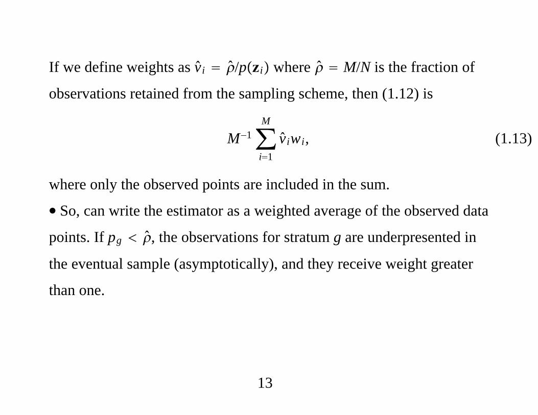
If we define weights as vi /pzi where M/N is the fraction of

observations retained from the sampling scheme, then (1.12) is

M−1∑i1

M

viwi, (1.13)

where only the observed points are included in the sum.

∙ So, can write the estimator as a weighted average of the observed data

points. If pg , the observations for stratum g are underpresented in

the eventual sample (asymptotically), and they receive weight greater

than one.

13

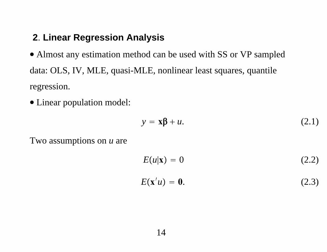
2. Linear Regression Analysis

∙ Almost any estimation method can be used with SS or VP sampled

data: OLS, IV, MLE, quasi-MLE, nonlinear least squares, quantile

regression.

∙ Linear population model:

y x u. (2.1)

Two assumptions on u are

Eu|x 0 (2.2)

Ex′u 0. (2.3)

14

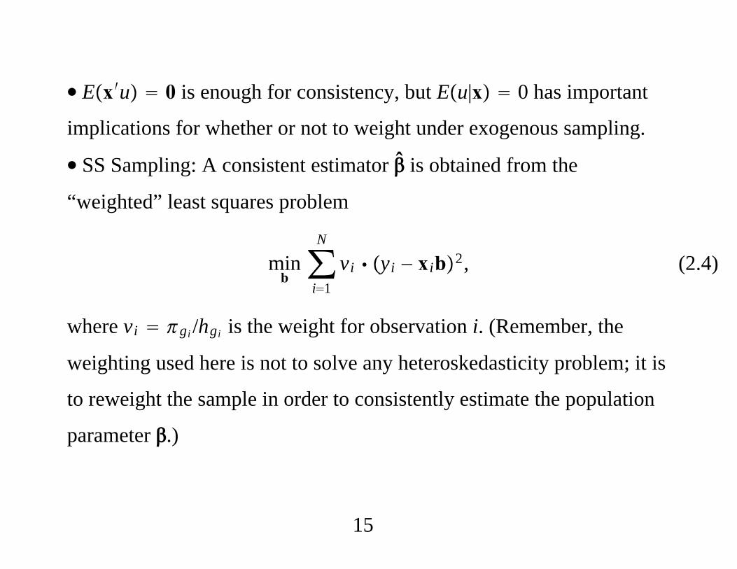
∙ Ex′u 0 is enough for consistency, but Eu|x 0 has important

implications for whether or not to weight under exogenous sampling.

∙ SS Sampling: A consistent estimator is obtained from the

“weighted” least squares problem

minb∑i1

N

vi yi − xib2, (2.4)

where vi gi /hgi is the weight for observation i. (Remember, the

weighting used here is not to solve any heteroskedasticity problem; it is

to reweight the sample in order to consistently estimate the population

parameter .)

15

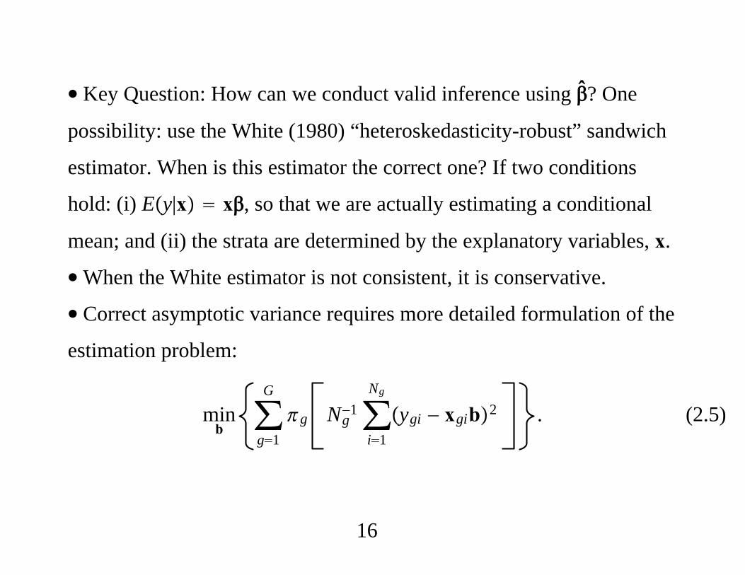
∙ Key Question: How can we conduct valid inference using ? One

possibility: use the White (1980) “heteroskedasticity-robust” sandwich

estimator. When is this estimator the correct one? If two conditions

hold: (i) Ey|x x, so that we are actually estimating a conditional

mean; and (ii) the strata are determined by the explanatory variables, x.

∙When the White estimator is not consistent, it is conservative.

∙ Correct asymptotic variance requires more detailed formulation of the

estimation problem:

minb∑g1

G

g Ng−1∑

i1

Ng

ygi − xgib2 . (2.5)

16

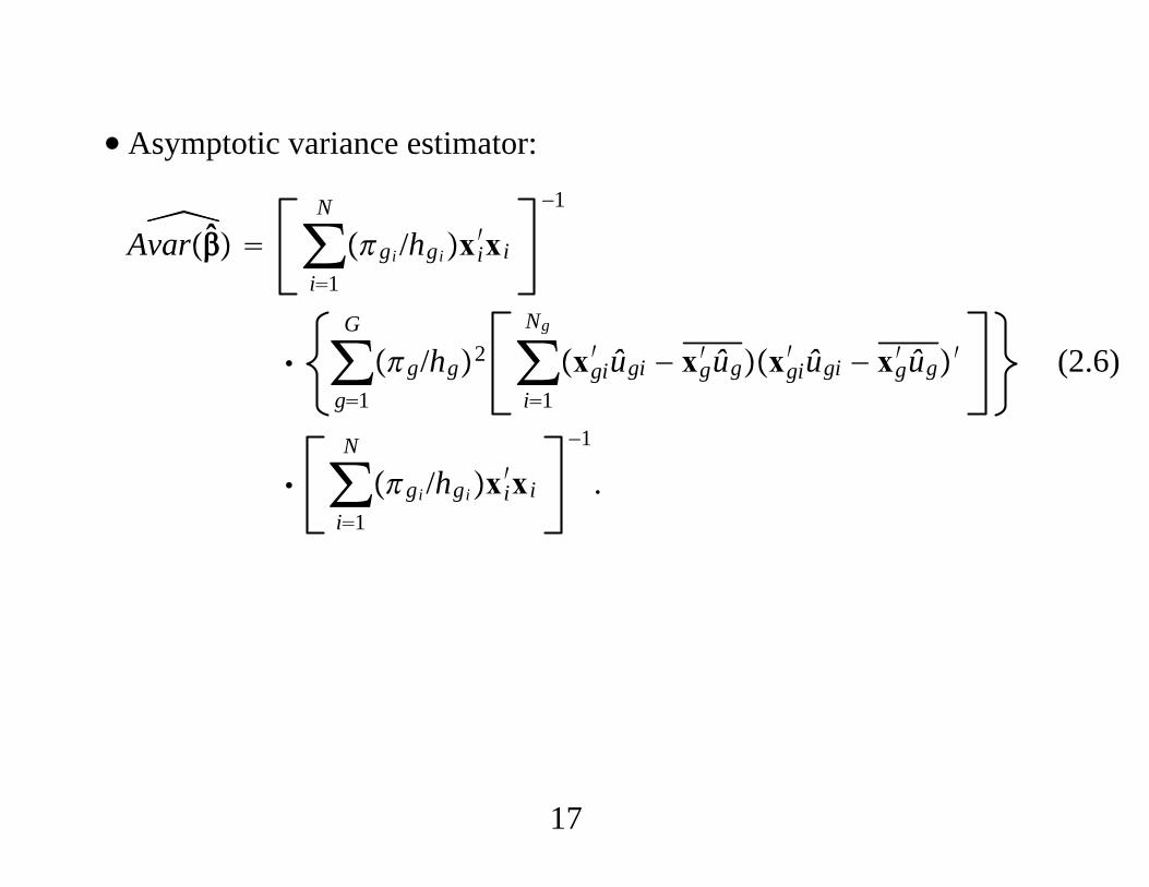
∙ Asymptotic variance estimator:

Avar ∑i1

N

gi /hgixi′xi

−1

∑g1

G

g/hg2 ∑i1

Ng

xgi′ ûgi − xg

′ ûgxgi′ ûgi − xg

′ ûg′

∑i1

N

gi /hgixi′xi

−1

.

(2.6)

17

∙ Usual White estimator ignores the information on the strata of the

observations, which is the same as dropping the within-stratum

averages, xg′ ûg. The estimate in (2.6) is always smaller than the usual

White estimate.

∙ Econometrics packages, such as Stata, have survey sampling options

that will compute (2.6) provided stratum membership is included along

with the weights. If only the weights are provided, the larger

asymptotic variance is computed.

18

∙ One case where there is no gain from subtracting within-strata means

is when Eu|x 0 and stratification is based on x.

∙ If we add the homoskedasticity assumption Varu|x 2 with

Eu|x 0 and stratification is based on x, the weighted estmator is less

efficient than the unweighted estimator. (Both are consistent.)

19

∙ The debate about whether or not to weight centers on two facts: (i)

The efficiency loss of weighting when the population model satisfies

the classical linear model assumptions and stratification is exogenous.

(ii) The failure of the unweighted estimator to consistently estimate if

we only assume

y x u, Ex′u 0, (2.7)

even when stratification is based on x. The weighted estimator

consistently estimates under (2.7).

20

∙ Analogous results hold for maximum likelihood, quasi-MLE,

nonlinear least squares, instrumental variables. If one knows stratum

identification along with the weights, the appropriate asymptotic

variance matrix (which subtracts off within-stratum means of the score

of the objective function) is smaller than the form derived by White

(1982). For, say, MLE, if the density of y given x is correctly specified,

and stratification is based on x, it is better not to weight. (But there are

cases – including certain treatment effect estimators – where it is

important to estimate the solution to a misspecified population

problem.)

21

∙ Findings for SS sampling have analogs for VP sampling, and some

additional results.

1. The Huber-White sandwich matrix applied to the weighted objective

function (weighted by the 1/pg) is consistent when the known pg are

used.

2. An asymptotically more efficient estimator is available when the

retention frequencies, pg Mg/Ng, are observed, where Mg is the

number of observed data points in stratum g and Ng is the number of

times stratum g was sampled. (Is Ng known? It could be.)

22

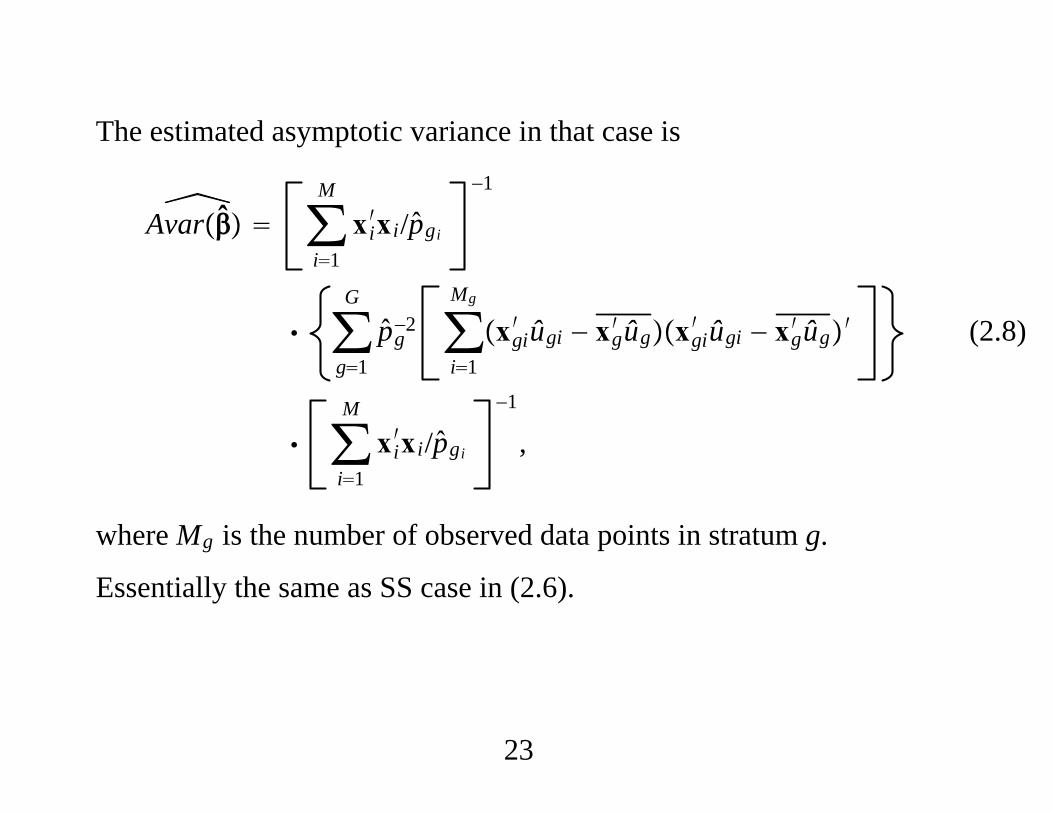
The estimated asymptotic variance in that case is

Avar ∑i1

M

xi′xi/pgi

−1

∑g1

G

pg−2 ∑

i1

Mg

xgi′ ûgi − xg

′ ûgxgi′ ûgi − xg

′ ûg′

∑i1

M

xi′xi/pgi

−1

,

(2.8)

where Mg is the number of observed data points in stratum g.

Essentially the same as SS case in (2.6).

23

∙ If we use the known sampling weights, we drop xg′ ûg from (2.8). If

Eu|x 0 and the sampling is exogenous, we also drop this term

because Ex′u|w ∈ Wg 0 for all g, and this is whether or not we

estimate the pg.

∙ In Stata, use the “svyset” command, and then the “svy” prefix for

sample statistics and econometric methods.

∙ Following example is with 6 strata and variable probability sampling

in addition to different strata weights. (Within each stratum, VP

sampling is used.)

24

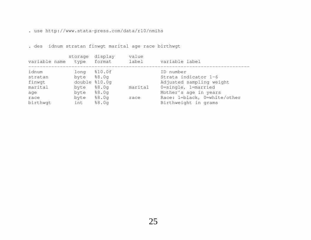
. use http://www.stata-press.com/data/r10/nmihs

. des idnum stratan finwgt marital age race birthwgt

storage display valuevariable name type format label variable label-----------------------------------------------------------------------------idnum long %10.0f ID numberstratan byte %8.0g Strata indicator 1-6finwgt double %10.0g Adjusted sampling weightmarital byte %8.0g marital 0single, 1marriedage byte %8.0g Mother’s age in yearsrace byte %8.0g race Race: 1black, 0white/otherbirthwgt int %8.0g Birthweight in grams

25

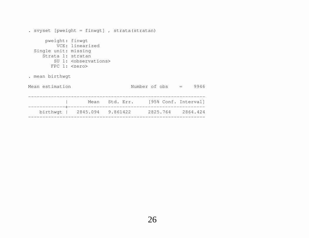
. svyset [pweight finwgt] , strata(stratan)

pweight: finwgtVCE: linearized

Single unit: missingStrata 1: stratan

SU 1: observationsFPC 1: zero

. mean birthwgt

Mean estimation Number of obs 9946

--------------------------------------------------------------| Mean Std. Err. [95% Conf. Interval]

-------------------------------------------------------------birthwgt | 2845.094 9.861422 2825.764 2864.424

--------------------------------------------------------------

26

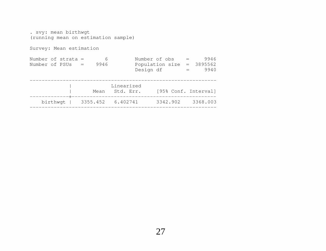
. svy: mean birthwgt(running mean on estimation sample)

Survey: Mean estimation

Number of strata 6 Number of obs 9946Number of PSUs 9946 Population size 3895562

Design df 9940

--------------------------------------------------------------| Linearized| Mean Std. Err. [95% Conf. Interval]

-------------------------------------------------------------birthwgt | 3355.452 6.402741 3342.902 3368.003

--------------------------------------------------------------

27

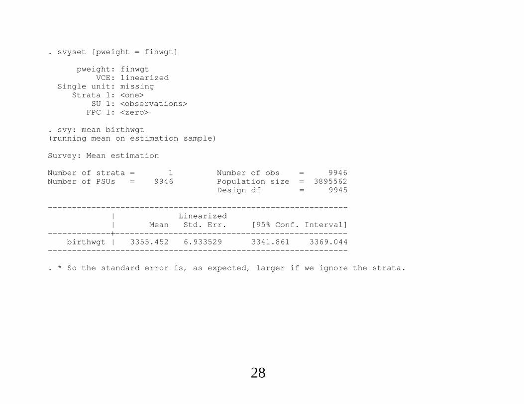
. svyset [pweight finwgt]

pweight: finwgtVCE: linearized

Single unit: missingStrata 1: one

SU 1: observationsFPC 1: zero

. svy: mean birthwgt(running mean on estimation sample)

Survey: Mean estimation

Number of strata 1 Number of obs 9946Number of PSUs 9946 Population size 3895562

Design df 9945

--------------------------------------------------------------| Linearized| Mean Std. Err. [95% Conf. Interval]

-------------------------------------------------------------birthwgt | 3355.452 6.933529 3341.861 3369.044

--------------------------------------------------------------

. * So the standard error is, as expected, larger if we ignore the strata.

28

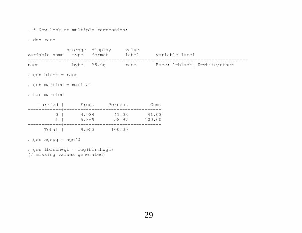
. * Now look at multiple regression:

. des race

storage display valuevariable name type format label variable label-------------------------------------------------------------------------------race byte %8.0g race Race: 1black, 0white/other

. gen black race

. gen married marital

. tab married

married | Freq. Percent Cum.-----------------------------------------------

0 | 4,084 41.03 41.031 | 5,869 58.97 100.00

-----------------------------------------------Total | 9,953 100.00

. gen agesq age^2

. gen lbirthwgt log(birthwgt)(7 missing values generated)

29

. svyset [pweight finwgt], strata(stratan)

pweight: finwgtVCE: linearized

Single unit: missingStrata 1: stratan

SU 1: observationsFPC 1: zero

. svy: reg lbirthwgt age agesq black married(running regress on estimation sample)

Survey: Linear regression

Number of strata 6 Number of obs 9946Number of PSUs 9946 Population size 3895561.7

Design df 9940F( 4, 9937) 300.19Prob F 0.0000R-squared 0.0355

------------------------------------------------------------------------------| Linearized

lbirthwgt | Coef. Std. Err. t P|t| [95% Conf. Interval]-----------------------------------------------------------------------------

age | .0094712 .0034286 2.76 0.006 .0027504 .0161919agesq | -.0001499 .0000634 -2.36 0.018 -.0002742 -.0000256black | -.074903 .0039448 -18.99 0.000 -.0826356 -.0671703

married | .0377781 .0058039 6.51 0.000 .0264013 .0491548_cons | 7.941929 .0442775 179.37 0.000 7.855136 8.028722

------------------------------------------------------------------------------

30

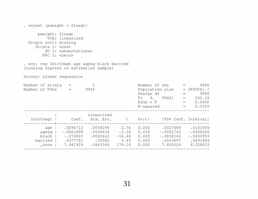
. svyset [pweight finwgt]

pweight: finwgtVCE: linearized

Single unit: missingStrata 1: one

SU 1: observationsFPC 1: zero

. svy: reg lbirthwgt age agesq black married(running regress on estimation sample)

Survey: Linear regression

Number of strata 1 Number of obs 9946Number of PSUs 9946 Population size 3895561.7

Design df 9945F( 4, 9942) 202.34Prob F 0.0000R-squared 0.0355

------------------------------------------------------------------------------| Linearized

lbirthwgt | Coef. Std. Err. t P|t| [95% Conf. Interval]-----------------------------------------------------------------------------

age | .0094712 .0034294 2.76 0.006 .0027489 .0161935agesq | -.0001499 .0000634 -2.36 0.018 -.0002743 -.0000256black | -.074903 .0045443 -16.48 0.000 -.0838106 -.0659953

married | .0377781 .00582 6.49 0.000 .0263697 .0491864_cons | 7.941929 .0443344 179.14 0.000 7.855024 8.028833

------------------------------------------------------------------------------

31

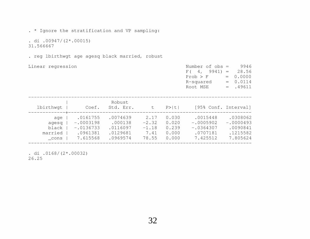
. * Ignore the stratification and VP sampling:

. di .00947/(2*.00015)31.566667

. reg lbirthwgt age agesq black married, robust

Linear regression Number of obs 9946F( 4, 9941) 28.56Prob F 0.0000R-squared 0.0114Root MSE .49611

------------------------------------------------------------------------------| Robust

lbirthwgt | Coef. Std. Err. t P|t| [95% Conf. Interval]-----------------------------------------------------------------------------

age | .0161755 .0074639 2.17 0.030 .0015448 .0308062agesq | -.0003198 .000138 -2.32 0.020 -.0005902 -.0000493black | -.0136733 .0116097 -1.18 0.239 -.0364307 .0090841

married | .0961381 .0129681 7.41 0.000 .0707181 .1215582_cons | 7.615568 .0969574 78.55 0.000 7.425512 7.805624

------------------------------------------------------------------------------

. di .0168/(2*.00032)26.25

32

∙ Little changes if we allow endogenous explanatory variables in the

population model:

y x uEz′u 0

∙ From a technical point of view, the estimator is a weighted 2SLS

estimator. Or, an optimal weighting matrix can be used in weighted

GMM.

∙ In Stata, the prefix svy: supports ivreg, too.

33

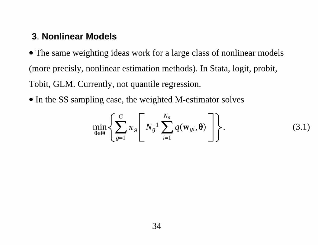
3. Nonlinear Models

∙ The same weighting ideas work for a large class of nonlinear models

(more precisly, nonlinear estimation methods). In Stata, logit, probit,

Tobit, GLM. Currently, not quantile regression.

∙ In the SS sampling case, the weighted M-estimator solves

min∈Θ∑g1

G

g Ng−1∑

i1

Ng

qwgi, . (3.1)

34

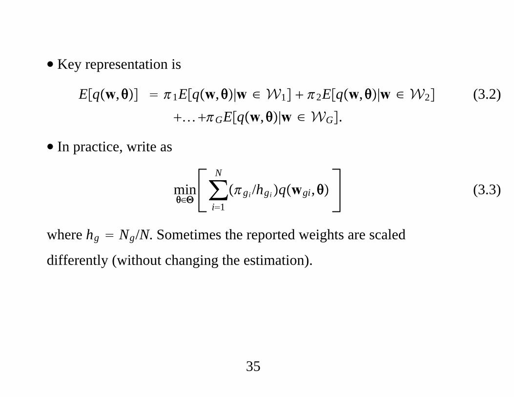
∙ Key representation is

Eqw, 1Eqw,|w ∈ W1 2Eqw,|w ∈ W2

…GEqw,|w ∈ WG. (3.2)

∙ In practice, write as

min∈Θ∑i1

N

gi /hgiqwgi, (3.3)

where hg Ng/N. Sometimes the reported weights are scaled

differently (without changing the estimation).

35

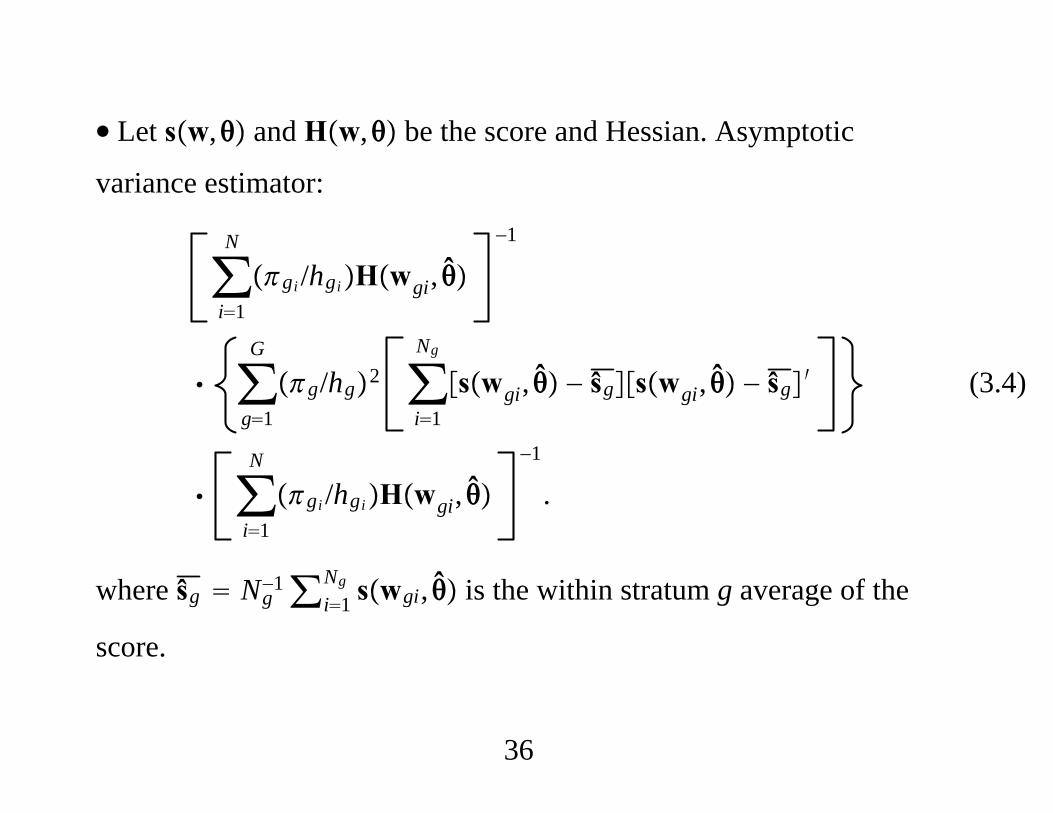
∙ Let sw, and Hw, be the score and Hessian. Asymptotic

variance estimator:

∑i1

N

gi /hgiHwgi, −1

∑g1

G

g/hg2 ∑i1

Ng

swgi, − ŝgswgi, − ŝg ′

∑i1

N

gi /hgiHwgi, −1

.

(3.4)

where ŝg Ng−1∑i1

Ng swgi, is the within stratum g average of the

score.

36

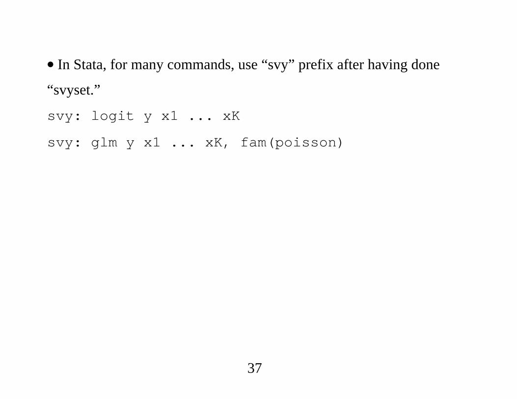
∙ In Stata, for many commands, use “svy” prefix after having done

“svyset.”

svy: logit y x1 ... xK

svy: glm y x1 ... xK, fam(poisson)

37

4. General Treatment of Exogenous Stratification

∙ Suppose our population model specifies some feature of Dy|x.

Could be a full distribution or a conditional mean.

∙ To ensure we consistently estimate the solution, say ∗, to the

population problem

min∈Θ

Eqw,,

we should use weights whether or not stratification is based on

conditioning variables x.

38

∙ This is important if we want to recover the “best” approximation to

the true underlying model. For example, if we want to estimate ∗ that

provides the best mean square approximation to Ey|x using

misspecified nonlinear least squares, we should use weighting even if it

is based only on x.

∙Wanting to estimate the solution to the population problem is exactly

what is needed for the “double robustness” result for treatment effect

estimation using regression plus propensity score weighting.

39

∙ However, if we assume that the feature of Dy|x is correctly

specified, we have chosen an appropriate objective function, and the

stratification is based on x, weighting – whether for SS or VP sampling

– is not needed for consistency and can be harmful in terms of

efficiency.

40

∙ For a general treatment, we assume that o solves

min∈Θ

Eqw,|x, (4.1)

for all x. This holds for conditional MLE when the model of the

density, fy|x;, is correctly specified. It holds for nonlinear least

squares with a correctly specified mean. It holds for quasi-MLE in the

linear exponential family (LEF) Ey|x is correctly specified. Also

holds for quantile regression when the conditional quantile function is

correctly specified.

41

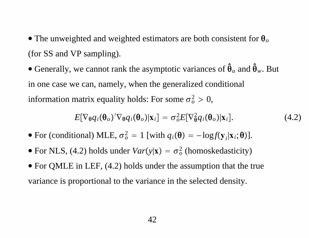
∙ The unweighted and weighted estimators are both consistent for o

(for SS and VP sampling).

∙ Generally, we cannot rank the asymptotic variances of u and w. But

in one case we can, namely, when the generalized conditional

information matrix equality holds: For some o2 0,

E∇qio′∇qio|xi o2E∇2qio|xi. (4.2)

∙ For (conditional) MLE, o2 1 [with qi − log fyi|xi;].

∙ For NLS, (4.2) holds under Vary|x o2 (homoskedasticity)

∙ For QMLE in LEF, (4.2) holds under the assumption that the true

variance is proportional to the variance in the selected density.

42

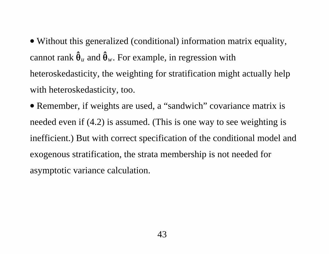
∙Without this generalized (conditional) information matrix equality,

cannot rank u and w. For example, in regression with

heteroskedasticity, the weighting for stratification might actually help

with heteroskedasticity, too.

∙ Remember, if weights are used, a “sandwich” covariance matrix is

needed even if (4.2) is assumed. (This is one way to see weighting is

inefficient.) But with correct specification of the conditional model and

exogenous stratification, the strata membership is not needed for

asymptotic variance calculation.

43

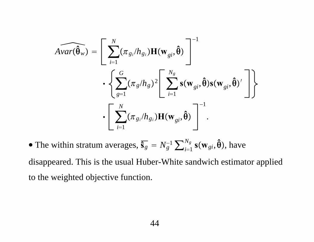
Avarw ∑i1

N

gi /hgiHwgi, −1

∑g1

G

g/hg2 ∑i1

Ng

swgi, swgi, ′

∑i1

N

gi /hgiHwgi, −1

.

∙ The within stratum averages, ŝg Ng−1∑i1

Ng swgi, , have

disappeared. This is the usual Huber-White sandwich estimator applied

to the weighted objective function.

44