Continuous-time impurity solvers

Philipp Werner

Theoretische Physik, ETH Zurich, 8093 Zurich, Switzerland

(Dated: May 2011)

I. QUANTUM IMPURITY MODELS

An quantum impurity model describes an atom or molecule embedded in some host or

bath, with which it can exchange electrons. This exchange of electrons allows the impurity

to make transitions between different quantum states, and leads to a non-trivial dynamics.

Quantum impurity models play a prominent role in nano-science as representations of quan-

tum dots or molecular conductors. They also serve as auxiliary problems, whose solution

yields the “dynamical mean field” description of correlated lattice models.

The Hamiltonian of a quantum impurity model contains three terms,

H = Hloc +Hbath +Hmix. (1)

Hloc describes the impurity, characterized by a small number of degrees of freedom (typically

spin and orbital degrees of freedom, which we denote by a, b, . . .), Hbath describes an infinite

reservoir of free electrons, labeled by a continuum of quantum numbers p and a discrete set

of quantum numbers ν (e. g. spin). Hmix describes the exchange of electrons between the

impurity and the bath in terms of hybridization amplitudes V aνp . Explicitly, the three terms

are

Hloc =∑

ab

Eabd†adb +∑

abcd

Uabcdd†ad†bdcdd, (2)

Hbath =∑

p,ν

ǫbpa†p,νap,ν , (3)

Hmix =∑

p,a,ν

(V a,νp d†aap,ν + h.c.). (4)

We will concentrate in the following on the “one-orbital Anderson model” (AIM), a

simplified representation of a magnetic impurity in a metallic host. In the AIM, the discrete

quantum number labelling the impurity or bath state is the spin σ, so the Hilbert space of

2

2

ε ε∼ ∼1 2U,

U,−V −t−t

p

p

1. . .

. . .

V

ε

µ

µ

FIG. 1: Left: Schematic representation of an AIM. Spin up and down electrons on the impurity

(black dot) interact with an on-site energy U and can hop to a continuum of non-interacting

bath levels with energy ǫp. The amplitudes for these transitions are given by the hybridization

parameters V ∗p . Right: Chain representation of the AIM. All the hopping parameters can be chosen

negative by a suitable gauge transformation.

the local problem Hloc = H0 +HU ,

H0 = −µ(n↑ + n↓), (5)

HU = Un↑n↓, (6)

has dimension four, and the bath and mixing terms are given by

Hbath =∑

p,σ

ǫpa†p,σap,σ, (7)

Hmix =∑

p,σ

(V σp d

†σap,σ + h.c.). (8)

An illustration of the AIM is shown in the left hand panel of Fig. 1.

A. Chain representation

The AIM (5)-(8) can be mapped onto a semi-infinite chain, with the first site corre-

sponding to the impurity. This mapping corresponds to a transformation of the operators

(d, ap1, ap2

, . . .) to new operators (d, c1, c2, . . .) such that H0 +Hbath +Hmix becomes tridiag-

onal.

3

−µ Vp1Vp2

Vp3. . .

V ∗p1

ǫp1

V ∗p2

ǫp2

V ∗p2

ǫp3

. . . . . .

→

−µ −V

−V ǫ1 −t1

−t1 ǫ2 −t2

−t2 ǫ3 . . .

. . . . . .

(9)

In the chain representation, the impurity orbital remains unchanged, and the hopping term

from the impurity to the first site of the chain is given by V = (∑

p |Vp|2)1/2. The phase

factors in this transformation can be chosen such that all the hopping terms are positive

(V > 0, ti > 0, i = 1, 2, . . .).

B. Action formulation

We may integrate out the bath degrees of freedom and express the partition function of

the AIM as

Z = TrTe−S (10)

with action S = Shyb + Sloc given by

Shyb =∑

σ

∫ β

0

dτdτ ′d†σ(τ)∆σ(τ − τ ′)dσ(τ′), (11)

Sloc =

∫ β

0

dτ [−µ(n↑(τ) + n↓(τ)) + Un↑(τ)n↓(τ)]. (12)

The hybridization function ∆σ(τ−τ ′) in Eq. (11) represents the amplitude for hopping from

the impurity into the bath at time τ ′ and back onto the impurity at time τ . It is a function of

the bath level energies and hybridization amplitudes, which is most conveniently expressed

in frequency space (iωn = (2n+ 1)π/β):

∆σ(iωn) =∑

p

|V σp |2

iωn − ǫp. (13)

It is also sometimes useful to introduce the noninteracting bath Green’s function G0 defined

as

G−10,σ(iωn) = iωn + µ− ∆σ(iωn). (14)

4

J t

effh

*Vp

FIG. 2: Mapping of the classical Ising model to a single-site effective model in static mean field

theory (left panel) and mapping of the Hubbard model to a quantum impurity model in dynamical

mean field theory (right panel).

II. DYNAMICAL MEAN FIELD THEORY

Quantum impurity models are a key ingredient in the dynamical mean field (DMFT)

formalism, which provides an approximate description of correlated lattice models. The

success of DMFT has created a demand for powerful and flexible impurity solvers and

triggered the development of the continuous-time solvers discussed in this chapter. We

will thus briefly introduce the DMFT approximation, which maps an interacting lattice

model, such as the one-band Hubbard model onto an effective single-site problem plus a

self-consistency condition.

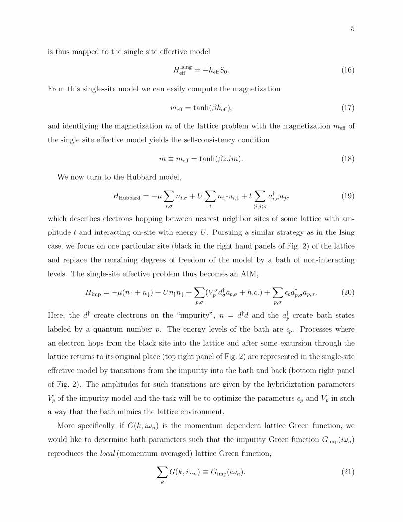
To appreciate the basic strategy, it is useful to briefly recall the static mean-field approx-

imation of the classical Ising model, which is illustrated in the left hand panel of Fig. 2.

Here, one focuses on a particular spin of the lattice, S0, and replaces the remaining degrees

of freedom by an effective external magnetic field heff = zJm (z is the coordination number

and m the magnetization per site). The lattice system

H Ising = −J∑

〈ij〉SiSj (15)

5

is thus mapped to the single site effective model

H Isingeff = −heffS0. (16)

From this single-site model we can easily compute the magnetization

meff = tanh(βheff), (17)

and identifying the magnetization m of the lattice problem with the magnetization meff of

the single site effective model yields the self-consistency condition

m ≡ meff = tanh(βzJm). (18)

We now turn to the Hubbard model,

HHubbard = −µ∑

i,σ

ni,σ + U∑

i

ni,↑ni,↓ + t∑

〈i,j〉σa†i,σajσ (19)

which describes electrons hopping between nearest neighbor sites of some lattice with am-

plitude t and interacting on-site with energy U . Pursuing a similar strategy as in the Ising

case, we focus on one particular site (black in the right hand panels of Fig. 2) of the lattice

and replace the remaining degrees of freedom of the model by a bath of non-interacting

levels. The single-site effective problem thus becomes an AIM,

Himp = −µ(n↑ + n↓) + Un↑n↓ +∑

p,σ

(V σp d

†σap,σ + h.c.) +

∑

p,σ

ǫpa†p,σap,σ. (20)

Here, the d† create electrons on the “impurity”, n = d†d and the a†p create bath states

labeled by a quantum number p. The energy levels of the bath are ǫp. Processes where

an electron hops from the black site into the lattice and after some excursion through the

lattice returns to its original place (top right panel of Fig. 2) are represented in the single-site

effective model by transitions from the impurity into the bath and back (bottom right panel

of Fig. 2). The amplitudes for such transitions are given by the hybridiztation parameters

Vp of the impurity model and the task will be to optimize the parameters ǫp and Vp in such

a way that the bath mimics the lattice environment.

More specifically, if G(k, iωn) is the momentum dependent lattice Green function, we

would like to determine bath parameters such that the impurity Green function Gimp(iωn)

reproduces the local (momentum averaged) lattice Green function,

∑

k

G(k, iωn) ≡ Gimp(iωn). (21)

6

A. DMFT approximation

The solution to Eq. (21) is computed iteratively and these DMFT iterations involve as

the essential approximation of the method a simplification of the momentum-dependence of

the lattice self-energy. The self-energy describes the effect of interactions on the propagation

of electrons. In the non-interacting model (U = 0) the lattice Green function is given by

GU=0(k, ω) = [iωn +µ− ǫk]−1, with ǫk the Fourier transform of the hopping matrix, whereas

the Green function of the interacting model is given by G(k, ω) = [iωn+µ−ǫk−Σ(k, iωn)]−1.

Therefore Σ(k, iωn) = G−1U=0(k, iωn) −G(k, iωn)−1, and similarly the impurity self-energy is

given by Σimp(iωn) = G−1imp,U=0(iωn) −Gimp(iωn)−1. The DMFT approximation amounts to

identifying the lattice self-energy with the momentum-independent impurity self-energy,

Σ(k, iωn) ≈ Σimp(iωn). (22)

Using this approximation we can rewrite Eq. (21) as

∑

k

[iωn + µ− ǫk − Σimp(iωn)]−1 ≡ Gimp(iωn). (23)

Since both Gimp(iωn) and Σimp(iωn) depend on the impurity model parameters ǫp and Vp we

obtain a self-consistency condition for the impurity model.

B. DMFT self-consisteny loop

Starting from an arbitrary initial bath Green function G0(iωn) (for example the solution

of the noninteracting problem), one iterates the following steps until convergence is reached:

1. Solve the impurity problem, i. e. compute the Green function Gimp(iωn) for the given

“bath” G0(iωn),

2. Extract the self-energy of the impurity model: Σimp(iωn) = G−10 (iωn) −G−1

imp(iωn),

3. Identify the lattice self-energy with the impurity self-energy (Σ(k, iωn) = Σimp(iωn))

and compute the local lattice Green function Gloc(iωn) =∑

k[iωn + µ− Σimp(iωn)]−1,

4. Apply the DMFT self-consistency condition (Gloc(iωn) = Gimp(iωn)) and use this to

define a new “bath” G−10,new(iωn) = G−1

loc(iωn) + Σimp(iωn).

7

The computationally expensive step in this procedure is the solution of the impurity

problem. Once the calculation has converged, the bath contains information about the

topology of the lattice. The impurity, which exchanges electrons with the bath, will thus

feel (at least to some extent) as if it were a site of the lattice. Obviously, not all the physics

can be captured by a single-site impurity model. In particular spatial fluctuations, which

become important in low-dimensional systems, are completely neglected. Dynamical mean

field calculations become exact in the limit of infinite dimension or coordination number, in

the non-interacting limit (U = 0) and in the atomic limit (t = 0).

C. Simulation of strongly correlated materials

The DMFT formalism can describe band-like behavior (quasi-particle peaks) and atomic-

like behavior (Hubbard bands). It thus captures the competition between localization and

delocalization which plays a crucial role in the physics of strongly correlated materials.

In order to enable “ab-initio” simulations of real compounds, the dynamical mean field

framework can be combined with density functional theory in the LDA approximation. The

resulting formalism is called “LDA+DMFT”. The idea is to use the Kohn-Sham eigenvalues

ǫKSk in the self-consistency equation (23) instead of the dispersion of some tight-binding

model. However, by doing so one encounters a problem: while density functional theory in

the LDA approximation does not take into account all the correlation effects it captures some

of them. If we now explicitly describe the local interaction in the strongly correlated orbitals

via some U -term in an effective impurity model, some interaction contributions appear twice

and this “double counting” of interaction energy must be compensated by adding a double

counting correction EDC to the self-energy of the correlated orbitals. The self-consistency

condition thus becomes

∑

k

[iωn + µ− ǫKSk − Σimp(iωn) −EDC ]−1 ≡ Gimp(iωn). (24)

There is no clean and consistent solution to the double counting problem in LDA+DMFT.

In practice, one uses formulas like EDC = U〈n〉 with 〈n〉 the average occupancy.

Most material simulations will involve several bands, so that the Kohn-Sham eingenvalues

define a matrix HLDAk in Wannier orbital space. Only the d- or f -orbitals will be explicitly

treated in the impurity calculation and yield a self-energy. Thus Σimp will be a matrix of

8

the same size as HLDAk , but the only non-zero elements will be in the block corresponding to

the strongly correlated d− or f -orbitals. Similarly the double-counting correction will be a

diagonal matrix with non-zero elements only for the correlated orbitals. In the multi-orbital

case, one can use as doulbe counting correction EDC = 〈U〉〈ncorr〉, with 〈U〉 the average of

the interaction parameters of the (multiorbital) impurity problem and 〈ncorr〉 the average

occupancy of the correlated orbitals. This orbital-independent shift assures that the crystal-

field splittings in the LDA band structure are preserved by the double counting correction.

The chemical potential µ is adjusted such that the correct total number of electrons in the

correlated and uncorrelated orbitals is obtained.

III. CONTINUOUS-TIME IMPURITY SOLVERS - GENERAL RECIPE

Quantum impurity models are 0+1 dimensional quantum field theories and as such com-

putationally much more tractable than interacting lattice models. By “solving the impurity

model” we essentially mean computing the impurity Green function (0 < τ < β)

G(τ) = 〈Td(τ)d†(0)〉 =1

ZTr

[

e−(β−τ)Hde−τHd†]

, (25)

with Z = Tr[e−βH ], the impurity model partition function, β the inverse temperature, and

Tr = TrdTra the trace over the impurity and bath states.

Hamiltonian based methods such as exact diagonalization or numerical RG explicitly treat

a finite number of bath states, and are suitable for single orbital models. However, because

the number of bath states must be increased proportional to the number of orbitals, the

computational effort grows exponentially with system size, and requires severe truncations

of the bath already for two orbitals. Monte Carlo methods have the advantage that the

bath is integrated out and thus the (infinite) size of the bath Hilbert space does not affect

the simulation. While restricted to finite temperature, Monte Carlo methods are thus the

method of choice for the solution of large multi-orbital or cluster impurity problems.

We will discuss here two complementary continuous-time Monte Carlo techniques: (i)

a weak-coupling approach, which scales favorably with system size and allows the efficient

simulation of large impurity clusters, and (ii) a strong-coupling approach, which can handle

impurity models with strong interactions. For simplicity, we will focus on the single-orbital

AIM impurity model defined in Eqs. (5)-(8).

9

Continuous-time Monte Carlo algorithms are based on an expansion of the partition

function into a series of “diagrams” and the stochastic sampling of (collections) of these

diagrams. We represent the partition function as a sum (or, more precisely, integral) of

configurations c with weight wc,

Z =∑

c

wc, (26)

and implement a random walk c1 → c2 → c3 → . . . in configuration space in such a way that

each configuration can be reached from any other in a finite number of steps (ergodicity)

and that detailed balance is satisfied,

|wc1|p(c1 → c2) = |w2|p(c2 → c1). (27)

This assures that each configuration is visited with a probability proportional to |wc| and one

can thus obtain an estimate for the Green function from a finite number N of measurements:

G =

∑

cwcGc∑

cwc=

∑

c |wc|signcGc∑

c |wc|signc

=〈sign ·G〉MC

〈sign〉MC. (28)

The first step in the derivation is to rewrite the partition function as a time ordered

exponential using some interaction representation. We split the Hamiltonian into two parts,

H = H1 +H2 and define the time dependent operators in the interaction picture as O(τ) =

eτH1Oe−τH1. In a second step, the time ordered exponential is expanded into a power series,

Z = Tr[

e−βH1Te−R β

0dτH2(τ)

]

=

∞∑

n=0

∫ β

0

dτ1 . . .

∫ β

τn−1

dτnTr[

e−(β−τn)H1(−H2) . . . e−(τ2−τ1)H1(−H2)e

−τ1H1

]

, (29)

which is a representation of the partition function of the form (26), namely the sum of all

configurations c = {τ1, . . . , τn}, n = 0, 1, . . ., τi ∈ [0, β) with weight

wc = Tr[

e−(β−τn)H1(−H2) . . . e−(τ2−τ1)H1(−H2)e

−τ1H1

]

dτn. (30)

The weak-coupling continuous-time Monte Carlo approach is based on an expansion of

Z in powers of the interaction U , and on an interaction representation in which the time

evolution is determined by the quadratic part H0 + Hbath + Hmix of the Hamiltonian. The

complementary “strong-coupling” approach is based on an expansion of Z in powers of the

impurity-bath hybridization V , and an interaction representation in which the time evolution

is determined by the local part H0 +HU +Hbath of the Hamiltonian.

10

IV. WEAK-COUPLING APPROACH

The weak-coupling continuous time impurity solver employs an expansion of the partition

function in powers of H2 = HU . Equation (30) thus gives the weight of a configuration of

n interaction vertices. Since H1 = H − H2 = H0 + Hbath + Hmix is quadratic, we can use

Wick’s theorem to evaluate the trace. The result is a product of two determinants of n× n

matrices (one for each spin), whose elements are bath Green functions G0 evaluated at the

time intervals defined by the vertex positions:

wc

Z0

= (−Udτ)n 1

Z0

Tr[

e−(β−τn)H1n↑n↓ . . . e−(τ2−τ1)H1n↑n↓e

−τ1H1

]

= (−Udτ)n∏

σ

detM−1σ , (31)

(M−1σ )ij = G0,σ(τi − τj), (32)

with Z0 = Tr[e−βH1] the partition function of the noninteracting model.

At this point, we encounter a problem. In the paramagnetic phase, where G0,↑ = G0,↓,

the product of determinants is positive, which means that for repulsive interaction (U > 0),

odd perturbation orders yield negative weights. Except in the particle-hole symmetric case,

where one can show that odd perturbation orders vanish, this will result in a severe sign

problem. Fortunately, we can solve this sign problem by shifting the chemical potentials for

up and down spins in an appropriate way. We rewrite the interaction term as

HU =U

2

∑

s,σ

(nσ − ασ(s)) +U

2(n↑ + n↓) −

U

4, (33)

ασ(s) = 1/2 + σs(1/2 + δ). (34)

Here δ is some constant and s = ±1 an Ising variable. The constant −U/4 in Eq. (33)

is irrelevant, while the contribution U(n↑ + n↓)/2 can be absorbed into the noninteracting

Green function by shifting the chemical potential as µ → µ − U/2. Explicitly, we redefine

the bath Green function as G−10,σ = iωn + µ− ∆σ → G−1

0,σ = iωn + µ− U/2 − ∆σ.

The introduction of an Ising variable si at each vertex position τi enlarges the configu-

ration space exponentially. A configuration c now corresponds to a collection of Ising spin

variables on the imaginary time interval: c = {(τ1, s1), (τ2, s2), . . . , (τn, sn)}. The weight of

11

these configurations are

wc

Z0= (−Udτ/2)n

∏

σ

det M−1σ , (35)

(M−1σ )ij = G0,σ(τi − τj) − ασ(si)δij . (36)

The Ising variables are in fact not needed to cure the sign problem. They have been intro-

duced to symmetrize the interaction term and prevent ergodicity problems.

A. Sampling procedure and detailed balance

For ergodicity it is sufficient to insert/remove spins with random orientation at random

times, because this allows in principle to generate all possible configurations. Furthermore,

the random walk in configuration space must satisfy the detailed balance condition (27).

Splitting the probability to move from configuration ci to configuration cj into a probability

to propose the move and a probability to accept it,

p(ci → cj) = pprop(ci → cj)pacc(ci → cj), (37)

we arrive at the condition

pacc(ci → cj)

pacc(cj → ci)=pprop(cj → ci)

pprop(ci → cj)

|w(cj)|

|w(ci)|. (38)

There is some flexibility in choosing the proposal probabilities. A reasonable choice for the

insertion/removal of a spin is the following (illustrated in Fig. 3):

• Insertion

Pick a random time in [0, β) and a random direction for the new spin:

pprop(n→ n+ 1) = (1/2)(dτ/β),

• Removal

Pick a random spin: pprop(n+ 1 → n) = 1/(n+ 1).

For this choice, the ratio of acceptance probabilities becomes

pacc(n→ n+ 1)

pacc(n+ 1 → n)=

βU

n + 1

∏

σ=↑,↓

| det(M(n+1)σ )−1|

| det(M(n)σ )−1|

, (39)

and the random walk can thus be implemented for example on the basis of the Metropo-

lis algorithm, i.e. the proposed move from n to n ± 1 is accepted with probability

min[1, pacc(n→ n± 1)/pacc(n± 1 → n)].

12

β

0

0

β

FIG. 3: Local update in the continuous-time auxiliary field method. The dashed line represents the

imaginary time interval [0, β). We increase the perturbation order by adding a spin with random

orientation at a random time. The perturbation order is decreased by removing a randomly chosen

spin.

B. Determinant ratios and fast matrix updates

From Eq. (39) it follows that each update requires the calculation of a ratio of two

determinants. Computing the determinant of a matrix of size (n×n) is an O(n3) operation.

However, each insertion or removal of a spin merely changes one row and one column of the

matrix M−1σ . We will now show that it is therefore possible to evaluate the ratio in Eq. (39)

in a time O(n2) (insertion) or O(1) (removal).

The objects which are stored and manipulated during the simulation are, besides the lists

of the times {τi} and spins {si}, the matrices Mσ = (G0σ)−1. Inserting a spin adds a new

row and column to M−1σ . We define the blocks (omitting the σ index)

(M (n+1))−1 =

(M (n))−1 Q

R S

, M (n+1) =

P Q

R S

, (40)

where Q, R, S denote (n× 1), (1× n), and (1× 1) matrices, respectively, which contain the

contribution of the added spin. The determinant ratio needed for the acceptance/rejection

probability is then given by

det(M (n+1))−1

det(M (n))−1=

1

det S= S − [R][M (n)Q]. (41)

As we store M (n), computing the acceptance/rejection probability of an insertion move is

an O(n2) operation. If the move is accepted, the new matrix M (n+1) is computed out of

13

M (n), Q,R, and S, also in a time O(n2):

S = (S − [R][M (n)Q])−1, (42)

Q = −[M (n)Q]S, (43)

R = −S[RM (n)], (44)

P = N (n) + [M (n)Q]S[RM (n)]. (45)

It follows from Eq. (41) that the calculation of the determinant ratio for removing a spin is

O(1), since it is just element S, and from the above formulas we also immediately find the

elements of the reduced matrix:

M (n) = P −[Q][R]

S. (46)

C. Measurement of the Green function

To compute the contribution of a configuration c to the Green function, Gcσ(τ), we insert

in Eq. (??) a creation operator d† at time 0 and an annihilation operator d at time τ and

divide by wc. Wick’s theorem then leads to the expression

Gcσ(τ) = G0σ(iωn) −

∑

k

G0σ(τ − τk)∑

l

[Mσ]klG0σ(τl). (47)

The impurity Green function is obtained as G(τ) = 〈Gcσ(τ)〉MC .

It is possible to accumulate the Fourier components of the Green function directly. Using

translational invariance of the Green functions one finds

Gcσ(iωn) = G0σ(iωn) −G0σ(iωn)

∑

k,l

1

βeiωn(τk−τl)[Mσ]klG0σ(iωn), (48)

so that G(iωn) = G0(iωn) − 1β(G0(iωn))2

⟨∑

k,l eiωn(τk−τl)[Mσ]kl

⟩

MC. Note that because the

bath Green function has the high-frequency behavior G0(iωn) ∼ 1/iωn, the impurity Green

function will inherit the correct high-frequency tail.

D. Generalization - multiorbital and cluster impurity problems

The generalization of the weak-coupling method to impurity clusters is straight forward.

All we have to do is to add a site index to the interaction vertices (or auxiliary Ising spin

14

variables) and sample the vertices (spins) on a family of nsites imaginary time intervals. In

principle, the weak-coupling solver can also be used to simulate lattice models, since the

only difference to a multi-site impurity problem is the definition of the bath G0. However,

the O(β3) scaling is not competitive with the BSS algorithm.

General four fermion terms as in (2) are, at least in principle, also easily dealt with.

One simply expands the partition function in powers of all the interaction terms Uabcd. The

trace over the impurity and bath degrees of freedom then again yields a determinant of a

matrix whose size is equal to the total perturbation order. To reduce the sign problem, it is

advantageous to introduce auxiliary fields α and replace

∑

abcd

Uabcdd†ad†bdcdd → −

∑

abcd

Uabcd(d†adc − αac)(d†bdd − αbd), (49)

with an appropriate shift in the quadratic part of the Hamiltonian. However, in general,

it will not be possible to completely eliminate the sign problem by a suitable choice of the

paramters α. Furthermore, since the number of interaction terms grows like O(n4orbital) the

computational cost rapidly escalates. In practice, the strong coupling approach discussed in

the following section turns out to be a more suitable approach for single-site multi-orbital

problems with complex interaction terms.

V. STRONG-COUPLING APPROACH - EXPANSION IN THE

IMPURITY-BATH HYBRIDIZATION

A continuous-time Monte Carlo method, which is in many ways complementary to the

weak-coupling approach, is based on an expansion of the partition function in powers of the

impurity-bath hybridization V . Here, we decompose the Hamiltonian as H2 = Hmix and

H1 = H −H2 = H0 +HU +Hbath. Since H2 ≡ Hd†

2 +Hd2 =

∑

σ,p Vσp d

†σap,σ +

∑

σ,p′ Vσ∗p′ dσa

†p,σ

has two terms, corresponding to electrons hopping from the bath to the impurity and from

the impurity back to the bath, only even perturbation orders contribute to Eq. (29). Fur-

thermore, at perturbation order 2n only the (2n)!/(n!)2 terms corresponding to n creation

operators d† and n annihilation operators d will contribute. We can therefore write the

15

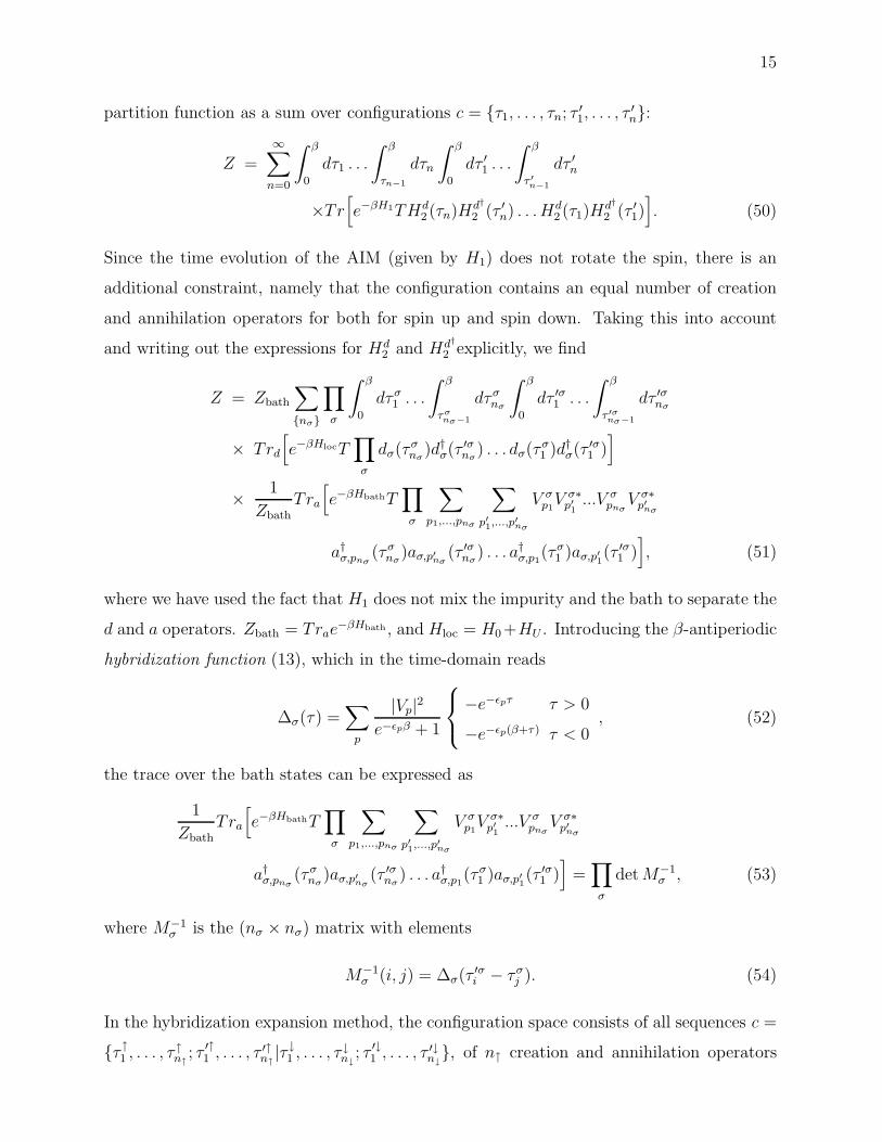
partition function as a sum over configurations c = {τ1, . . . , τn; τ ′1, . . . , τ′n}:

Z =∞

∑

n=0

∫ β

0

dτ1 . . .

∫ β

τn−1

dτn

∫ β

0

dτ ′1 . . .

∫ β

τ ′n−1

dτ ′n

×Tr[

e−βH1THd2 (τn)Hd†

2 (τ ′n) . . .Hd2 (τ1)H

d†

2 (τ ′1)]

. (50)

Since the time evolution of the AIM (given by H1) does not rotate the spin, there is an

additional constraint, namely that the configuration contains an equal number of creation

and annihilation operators for both for spin up and spin down. Taking this into account

and writing out the expressions for Hd2 and Hd†

2 explicitly, we find

Z = Zbath

∑

{nσ}

∏

σ

∫ β

0

dτσ1 . . .

∫ β

τσnσ−1

dτσnσ

∫ β

0

dτ ′σ1 . . .

∫ β

τ ′σnσ−1

dτ ′σnσ

× Trd

[

e−βHlocT∏

σ

dσ(τσnσ

)d†σ(τ′σnσ

) . . . dσ(τσ1 )d†σ(τ ′σ1 )

]

×1

ZbathTra

[

e−βHbathT∏

σ

∑

p1,...,pnσ

∑

p′1,...,p′nσ

V σp1V σ∗

p′1...V σ

pnσV σ∗

p′nσ

a†σ,pnσ(τσ

nσ)aσ,p′nσ

(τ ′σnσ) . . . a†σ,p1

(τσ1 )aσ,p′1

(τ ′σ1 )]

, (51)

where we have used the fact that H1 does not mix the impurity and the bath to separate the

d and a operators. Zbath = Trae−βHbath , and Hloc = H0+HU . Introducing the β-antiperiodic

hybridization function (13), which in the time-domain reads

∆σ(τ) =∑

p

|Vp|2

e−ǫpβ + 1

−e−ǫpτ τ > 0

−e−ǫp(β+τ) τ < 0, (52)

the trace over the bath states can be expressed as

1

ZbathTra

[

e−βHbathT∏

σ

∑

p1,...,pnσ

∑

p′1,...,p′nσ

V σp1V σ∗

p′1...V σ

pnσV σ∗

p′nσ

a†σ,pnσ(τσ

nσ)aσ,p′nσ

(τ ′σnσ) . . . a†σ,p1

(τσ1 )aσ,p′1

(τ ′σ1 )]

=∏

σ

detM−1σ , (53)

where M−1σ is the (nσ × nσ) matrix with elements

M−1σ (i, j) = ∆σ(τ ′σi − τσ

j ). (54)

In the hybridization expansion method, the configuration space consists of all sequences c =

{τ ↑1 , . . . , τ↑n↑

; τ ′↑1 , . . . , τ′↑n↑|τ ↓1 , . . . , τ

↓n↓

; τ ′↓1 , . . . , τ′↓n↓}, of n↑ creation and annihilation operators

16

overlap

0 β

0 βδ

l

l

l

max

new

FIG. 4: Local update in the “segment” picture. The two segment configurations correspond to spin

up and spin down. Each segment depicts a time interval in which an electron of the corresponding

spin resides on the impurity (the end points are the locations of the operators d† and d). We

increase the perturbation order by adding a segment or anti-segment of random length for random

spin. The perturbation order is decreased by removing a randomly chosen segment.

for spin up (n↑ = 0, 1, . . .), and n↓ creation and annihilation operators for spin down (n↓ =

0, 1, . . .). The weight of this configuration is

wc = ZbathTrd

[

e−βHlocT∏

σ

dσ(τσnσ

)d†σ(τ′σnσ

) . . . dσ(τσ1 )d†σ(τ

′σ1 )

]

×∏

σ

detM−1σ (τσ

1 , . . . , τσnσ

; τ ′σ1 , . . . , τ′σnσ

)(dτ)2nσ . (55)

The trace factor represents the contribution of the impurity, which fluctuates between dif-

ferent quantum states, as electrons hop in and out. The determinants resum all the bath

evolutions which are compatible with the given sequence of transitions (see Section ??).

To evaluate the trace factor, one may use the eigenbasis of Hloc. In this basis, the time

evolution operator e−τHloc is diagonal while the operators dσ and d†σ will produce transitions

between eigenstates with amplitude ±1.

Because the time evolution does not flip the spin, the creation and annihilation operators

for given spin have to alternate. This allows us to separate the operators for spin up from

those for spin down and to depict the time evolution by a collection of segments (each

segment representing a time interval in which an electron of spin up or down resides on

17

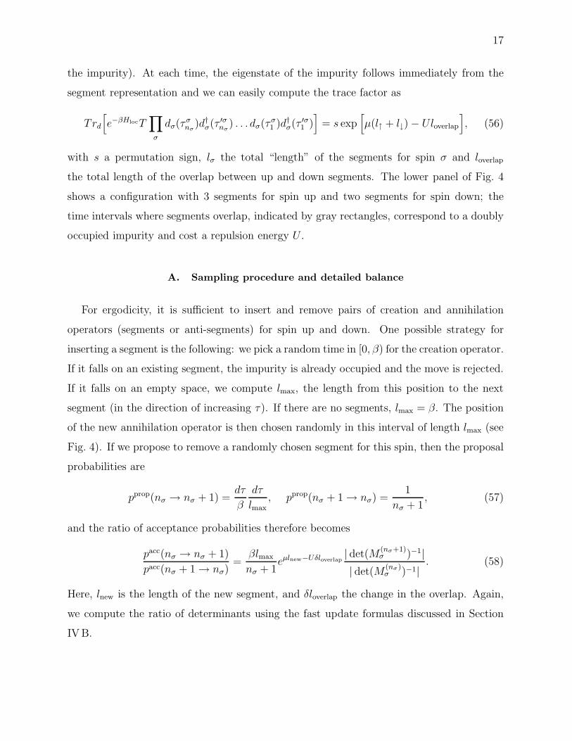
the impurity). At each time, the eigenstate of the impurity follows immediately from the

segment representation and we can easily compute the trace factor as

Trd

[

e−βHlocT∏

σ

dσ(τσnσ

)d†σ(τ ′σnσ) . . . dσ(τσ

1 )d†σ(τ ′σ1 )]

= s exp[

µ(l↑ + l↓) − Uloverlap

]

, (56)

with s a permutation sign, lσ the total “length” of the segments for spin σ and loverlap

the total length of the overlap between up and down segments. The lower panel of Fig. 4

shows a configuration with 3 segments for spin up and two segments for spin down; the

time intervals where segments overlap, indicated by gray rectangles, correspond to a doubly

occupied impurity and cost a repulsion energy U .

A. Sampling procedure and detailed balance

For ergodicity, it is sufficient to insert and remove pairs of creation and annihilation

operators (segments or anti-segments) for spin up and down. One possible strategy for

inserting a segment is the following: we pick a random time in [0, β) for the creation operator.

If it falls on an existing segment, the impurity is already occupied and the move is rejected.

If it falls on an empty space, we compute lmax, the length from this position to the next

segment (in the direction of increasing τ). If there are no segments, lmax = β. The position

of the new annihilation operator is then chosen randomly in this interval of length lmax (see

Fig. 4). If we propose to remove a randomly chosen segment for this spin, then the proposal

probabilities are

pprop(nσ → nσ + 1) =dτ

β

dτ

lmax, pprop(nσ + 1 → nσ) =

1

nσ + 1, (57)

and the ratio of acceptance probabilities therefore becomes

pacc(nσ → nσ + 1)

pacc(nσ + 1 → nσ)=

βlmax

nσ + 1eµlnew−Uδloverlap

| det(M(nσ+1)σ )−1|

| det(M(nσ)σ )−1|

. (58)

Here, lnew is the length of the new segment, and δloverlap the change in the overlap. Again,

we compute the ratio of determinants using the fast update formulas discussed in Section

IVB.

18

B. Measurement of the Green function

The strategy here is to create configurations which contribute to the Green function

measurement by decoupling the bath from a given pair of creation and annihilation operators

in c. The idea is to write

g(τ) =1

Z

∑

c

wd(τ)d†(0)c =

1

Z

∑

c

w(τ,0)c

wd(τ)d†(0)c

w(τ,0)c

, (59)

where wd(τ)d†(0)c denotes the weight of configuration c with and additional operator d†(0)

and d(τ) in the trace factor, and w(τ,0)c the complete weight corresponding to the enlarged

operator sequence (including enlarged hybridization determinants). Since the trace factors

of both weights are identical,

wd(τ)d†(0)c

w(τ,0)c

=detM−1

c

det(M(τ,0)c )−1

= (M (τ,0)c )j,i, (60)

with i and j denoting the row and column corresponding to the new operators d† and d in

the enlarged (M(τ,0)c )−1. Hence, the measurement formula for the Green function becomes

G(τ) =1

Z

∑

c

wc

∑

i,j

1

β∆(τ, τi − τ ′j)(Mc)ji =

⟨

∑

i,j

1

β∆(τ, τi − τ ′j)Mji

⟩

MC, (61)

with ∆(τ, τ ′) = δ(τ − τ ′) for τ ′ > 0, and ∆(τ, τ ′) = −δ(τ − τ ′ − β) for τ ′ < 0.

We may Fourier transform Eq. (61) to obtain a measurement formula for the Fourier

coefficients of the Green function,

G(iωn) =⟨

∑

i,j

1

βeiωn(τi−τ ′

j)Mji

⟩

MC. (62)

Note that in contrast to the weak-coupling approach, where the Green function is measured

as a O(1/(iωn)2) correction to the bath Green function, Eq. (62) does not automatically

yield the correct high frequency tails. It is thus advantageous to accumulate the coefficients

of an expansion of the Green function in Legendre polynomials.

C. Generalization - Matrix formalism

It is obvious from the derivation in Section V that the hybridization expansion formalism

is applicable to general classes of impurity models. Because the trace factor in the weight

19

(55) is computed exactly, Hloc can contain essentially arbitrary interactions (e. g. spin-

exchange terms in multi-orbital models), degrees of freedom (e. g. spins in Kondo-lattice

models) or constraints (e. g. no double occupancy in the t-J model).

For multi-orbital impurity models with density-density interaction, the segment formalism

is still applicable: we have now a collection of segments for each flavor α (orbital, spin) and

the trace factor can still be computed from the length of the segments (chemical potential

contribution) and the overlaps between segments of different flavor (interaction terms).

If Hloc is not diagonal in the occupation number basis defined by the d†α, the calcula-

tion of Trd

[

e−βHlocT∏

α dα(ταnα

)d†α(τ ′αnα) . . . dσ(τα

1 )d†α(τ ′α1 )]

becomes more involved. We now

have to compute the trace explicitly in some basis of Hloc – for example the eigenbasis, in

which the time evolution operators e−Hlocτ become diagonal. The operators dα and d†α are

expressed as matrices in this eigenbasis, and the evaluation of the trace factor thus involves

the multiplication of matrices whose size is equal the size of the Hilbert space of Hloc. Since

the dimension of the Hilbert space grows exponentially with the number of flavors, the cal-

culation of the trace factor becomes the computational bottleneck of the simulation, and

the matrix formalism is therefore restricted to a relatively small number of flavors (up to

about 10).

An important point is the use of conserved quantum numbers (typically particle num-

ber for spin up and spin down, momentum, . . . ). If the eigenstates of Hloc are grouped

according to these quantum numbers, the operator matrices will acquire a sparse block

structure, because for example d†↑,q will connect the states corresponding to quantum num-

bers m = {n↑, n↓, K} to those corresponding to m′ = {n↑ + 1, n↓, K + q} (if they exist).

Checking the compatibility of the operator sequence with a given starting block furthermore

allows one to find the (potentially) contributing quantum number sectors without any matrix

multiplications. The evaluation of the trace is thus reduced to a block matrix multiplication

of the form∑

contr.m

Trm

[

. . . (O)m′′,m′(e−(τ ′−τ)Hloc)m′(O)m′,m(e−τHloc)m

]

, (63)

where O is either a creation or annihilation operator, m denotes the index of the matrix

block, and the sum runs over those sectors which are compatible with the operator sequence.

20

VI. INFINITE-U LIMIT: KONDO MODEL

In the limit of very strong interaction, the half-filled AIM model cannot be simulated

efficiently using the weak or strong coupling continuous-time Monte Carlo solvers. The

weak-coupling approach is not suitable because the perturbation order becomes very large,

while in the strong-coupling simulation, hybridization events correspond to transitions into

doubly occupied or empty states with very high energy. While transitions into states with

occupancy different from one can still be accepted, as long as the excursion is very short,

and the strong-coupling code can in principle handle arbitrarily short “segments” or “anti-

segments”, it is more appropriate and more efficient to project out the charge fluctuations

and consider a low-energy effective model in which the singly occupied impurity (represented

by a spin S = 1/2) exchanges spin with the bath. This projection is called “Schrieffer-Wolf”

transformation and leads to the Kondo-Hamiltonian

H =∑

k,σ

ǫkc†kσckσ + JS · ψ†

c~σψc. (64)

Here, J is the exchange parameter of order V 2/U and ψ†c = (c†0,↑, c

†0,↓), where c0 is the first

bath site in a chain representation of the impurity (see Fig. 5). To solve this model, we have

to compute the Green function of the bath at site 0. The green function of the impurity

is then given by the T -matrix of the bath, as can be shown using equations of motion. In

the following sections we will discuss two complementary continuous-time solvers, a weak-

coupling approach based on an expansion in powers of J and a strong-couping approach

based on an expansion in powers of the hybridization between site 0 and the rest of the

bath.

A. Weak-coupling approach

In the weak-coupling simulation, we fermionize the spin S by introducing annihilation

operators fσ and writing

S =1

2ψ†

f~σψf , (65)

with ψ†f = (f †

↑ , f†↓). The hamiltonian (64) may then be written in the form

H =∑

k

ǫkc†kσckσ + J

[

Sz(c†↑c↑ − c†↓c↓) + S+c†↓c↑ + S−c†↑c↓

]

, (66)

21

−

−t−t1 2J −V

µ

. . .

ε ε∼ ∼1 2

FIG. 5: Chain representation of the quantum impurity model in the Kondo limit. The impurity

states are restricted to the singly occupied states | ↑〉 and | ↓〉. This spin-1/2 degree of freedom

couples via J to the spin ~S = ψ†c~σψc on lattice site 0, represented in the figure by the first site of

the chain.

with S+ = f †↑f↓, S

− = f †↓f↑ and Sz = 1

2(f †

↑f↑ − f †↓f↓). Adding and subtracting a term

J2(f †

↑f↑ + f †↓f↓) and using the constraint f †

↑f↑ + f †↓f↓ = 1, we finally obtain

H =∑

k

ǫkc†kσckσ −

J

2

∑

σ

c†0,σc0,σ + J∑

σσ′

f †σfσ′c†σ′cσ. (67)

We may now split the Hamiltonian into the exactly solved part H1 =∑

k ǫkc†kσckσ −

J2

∑

σ c†0,σc0,σ and expand the partition function into powers of H2 = J

∑

σσ′ f †σfσ′c†σ′cσ.

The trace over the fermionic degrees of freedom then yields the weight of the Monte Carlo

configuration,

w = (−Jdτ)kTrf

[

Tf †σ1

(τ1)fσ′1(τ1) . . . f

†σk

(τk)fσ′k(τk)

]

×∏

σ

1

Zc

Trc

[

Tc†σ(τ ′1)cσ(τ ′′1 ) . . . c†σ(τ ′kσ)cσ(τ ′′kσ

)]

s, (68)

with 0 < τ1 < . . . < τk < β the H2-operator positions, 0 < τ ′1 < . . . < τ ′kσ< β the locations

of the bath creation operators, 0 < τ ′′1 < . . . < τ ′′kσ< β the locations of the bath annihilation

operators (∑

σ kσ = k), s a permutation sign associated with the separation of the spin up

and down operators and the grouping into pairs of creation/annihilation operators, and Zc

the partition function for H1.

While the trace over the f -states imposes a constraint on which type of operators can

be inserted (either “diagonal operators” c†σcσ with σ identical to the spin of the f -fermion,

or pairs of spin flip operators c†↑c↓ or c†↓c↑), the trace over the c-states results in a product

of determinants of two matrices detM↑ detM↓. Due to the scattering term in Eq. (67),

the elements of these matrices are given by noninteracting Green functions G0,σ which are

22

up

down

downcc

ff up

FIG. 6: Monte Carlo configuration corresponding to four off-diagonal and six diagonal operators.

The upper two lines represent the time evolution of the f -states with σ =↑, ↓ (i.e. of the orientation

of the spin S). Full circles represent creation operators and empty circle annihilation operators.

The sequence of c0 creation and annihilation operators for spin up and down is shown on the lower

two lines (full and empty squares). A diagonal operator c†σ(τ)cσ(τ) can only be inserted if the spin

S is in state σ.

related to the bath Green functions G0,σ by

G0,σ(iωn) =G0,σ(iωn)

1 + J2G0,σ(iωn)

. (69)

Specifically, (Mσ)ij = G0,σ(τ ′′i − τj).

A possible sequence of operators is shown in Fig. 6, where the upper two time lines

represent the evolution of the spin, and the lower two time lines the sequence of bath

creation and annihilation operators. Creation and annihilation operators are represented

by full and empty squares, respectively. Half-full squares correspond to diagonal operators

c†σ(τ)cσ(τ), whose σ must be identical to the spin represented by the f -lines.

The Monte Carlo sampling proceeds via insertion and removal of pairs of spin flips (verti-

cal dashed lines in Fig. 6), and via insertion and removal of diagonal operators. The spin flip

updates are analogous to the segment configuration updates discussed in Sec. VA. We can

pick a random time for the first spin flip and define an interval lmax up to the next operator

(which may be a diagonal operator or a spin-flip event). The second spin flip is then chosen

on a random point on this interval. The removal of a pair of adjacent spin-flips is only

possible if there is no diagonal operator in between. The diagonal operators can be inserted

and removed individually, but the insertion is only possible if their spin is compatible with

23

the state of the f -line.

The measurement of the bath Green’s function in the localized orbital 0 on the other

hand, works as described in the weak-coupling Sec. IVC. This measurement amounts to the

accumulation of the t-matrix

tσ(iωn) =⟨

−1

β

∑

k,l

eiωn(τk−τl)[Mσ]kl

⟩

, (70)

where the tilde reminds us that this t-matrix is computed with respect to G0, and is related

to the Green function G and the true t-matrix by

Gσ(iωn) = G0,σ(iωn) + G0,σ(iωn)tσ(iωn)G0,σ(iωn)

= G0,σ(iωn) +G0,σ(iωn)tσ(iωn)G0,σ(iωn). (71)

Hence, the t-matrix of the bath is obtained from Eq. (70) as

tσ(iωn) =−J

2

1 + J2G0,σ(iωn)

+tσ(iωn)

(1 + J2G0,σ(iωn))2

. (72)

Using equations of motion, one can show that tσ(iωn) directly yields the impurity Green

function.

B. Strong-coupling approach

The model (64) may also be simulated efficiently using the strong-coupling method dis-

cussed in Sec. V. In this approach, the local part of the Hamiltonian,

Hloc = −µ∑

σ

c†0,σc0,σ + J~S ·1

2ψ†

c~σψc. (73)

is treated exactly and the partition function is expanded in powers of the hoppings from

and to the localized orbital 0 of the c-electrons (parameter V in Fig. 5).

Hloc can be diagonalized in a basis labeled by the total number of electrons, the total

spin and the z-component of the total spin. If the particle number is 0 or 2, then the spin

state is determined by the state of the local moment, if the number is 1, the spin state is

singlet (S) or triplet (Tmz) with mz = 1, 0 or −1. The eigenstates may thus be labeled as

shown in Tab. I, where the first entry is the number of electrons and the second entry refers

to the spin state. The singlet state is defined as S = 1√2(|↑, ↓〉 − |↓, ↑〉), with the first entry

24

Eigenstates Energy

|1〉 = |0, ↑〉 0

|2〉 = |0, ↓〉 0

|3〉 = |1, S〉 −34J − µ

|4〉 = |1, T1〉14J − µ

|5〉 = |1, T0〉14J − µ

|6〉 = |1, T−1〉14J − µ

|7〉 = |2, ↑〉 −2µ

|8〉 = |2, ↓〉 −2µ

TABLE I: Eigenstates and eigenenergies for the local part of the Kondo lattice hamiltonian. The

first entry labels the number of electrons and the second entry the spin state: either impurity spin

↑, ↓ if the number of electrons is 0 or 2 or the total spin S (singlet) Tm (triplet with mz = m) if

n = 1.

the conduction electron and the second entry the local moment spin direction. In this basis,

the time evolution operator is diagonal, K(τ)|n〉 = exp(−Enτ)|n〉, with eigenenergies En

listed in Tab. I. The creation operators for spin up and down become the sparse matrices

c†↑ =

0 0 0 0 0 0 0 0

0 0 0 0 0 0 0 0

0 1√2

0 0 0 0 0 0

1 0 0 0 0 0 0 0

0 1√2

0 0 0 0 0 0

0 0 0 0 0 0 0 0

0 0 −1√2

0 1√2

0 0 0

0 0 0 0 0 1 0 0

, (74)

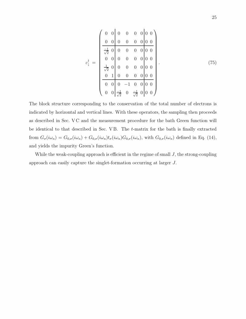
25

c†↓ =

0 0 0 0 0 0 0 0

0 0 0 0 0 0 0 0

−1√2

0 0 0 0 0 0 0

0 0 0 0 0 0 0 0

1√2

0 0 0 0 0 0 0

0 1 0 0 0 0 0 0

0 0 0 −1 0 0 0 0

0 0 −1√2

0 −1√2

0 0 0

. (75)

The block structure corresponding to the conservation of the total number of electrons is

indicated by horizontal and vertical lines. With these operators, the sampling then proceeds

as described in Sec. VC and the measurement procedure for the bath Green function will

be identical to that described in Sec. VB. The t-matrix for the bath is finally extracted

from Gσ(iωn) = G0,σ(iωn) + G0,σ(iωn)tσ(iωn)G0,σ(iωn), with G0,σ(iωn) defined in Eq. (14),

and yields the impurity Green’s function.

While the weak-coupling approach is efficient in the regime of small J , the strong-coupling

approach can easily capture the singlet-formation occurring at larger J .