continuous optimization problems and a polynomial ... · alternating operations of maximization and...

JOURNAL OF COMPLEXITY 1, 210-231 (1985)

Continuous Optimization Problems and a Polynomial Hierarchy of Real Functions*,’

KER-I Ko

Department of Computer Science, University of Houston, Houston, Texas 77004

The close connection between the maximization operation and nondeterministic computation has been observed in many different forms. We examine this relationship on real functions and give a characterization of NP-time computable real functions by the maximization operation. A natural extension of NP-time computable real functions to a polynomial hierarchy of real functions has a characterization by alternating operations of maximization and minimization. Although syntactically this hierarchy of real functions can be treated as a polynomial hierarchy of operators, the well-known Baker-Gill-Solovay separation result does not apply to this hierarchy. This phenomenon is explained by the inherent structural properties of real functions, and is compared with recent studies on positive relativization. B 1985 Academic FTCSS I I I C .

1. INTRODUCTION

In the study of the theory of NP-completeness, a great number of natural combinatorial optimization problems have been shown to be NP-complete. (See Garey and Johnson (1979) for a complete list.) Since all these optimization problems have the same computational complexity and similar structures, it is natural to try to study these problems uniformly in a general framework. For example, for the purpose of a theory of approximation algorithms, Johnson (1974) has given a general formulation of a class of optimization problems:

Given (a) a set D of problem instances, (b) for each instance I in D a finite set S(Z) of candidate solutions for I, and (c) for each solution u E S(Z) a positive rational number m (I, a), find for each

* Presented at the Symposium on Complexity of Approximately Solved Problems, April 17, 1985.

‘This research was supported in part by National Science Foundation Grants MCS-8103479 and MCS-8103479AOl.

210 0885-064X/85 $3.00 Copyright 0 1985 by Academic Press, Inc. All rights of reproduction in any form reserved.

POLYNOMIAL HIERARCHY OF REAL FUNCTIONS

2 in D the optimal solution U* E S(Z) such that m(Z, a*) is max- imized (or, minimized).

211

Often the size of the set S(Z) of solutions grows in an exponential rate as a function of the size of the instance I. Thus an exhaustive search algorithm would take time exponential in its input size. A good approximation algorithm should run in time polynomial in its input size and output a solution u E S(Z) with the value m(Z, a) close to the optimal value m(Z, a*).

A more abstract formulation for the general maximization problem is the following:

For a given polynomial-time computable function f: N + N and a given integer x E N, find max {f(y): y 5 x}.

More precisely, we ask whether the function maxf, defined by max# = max{f( y): y 5 x}, is polynomial-time computable, provided thatfis known to be polynomial-time computable. From the study of NP-complete combinatorial optimization problems, we naturally expect that the above question has an affirmative answer iff P = NP. Indeed, this is the case, as proved by Friedman (1984).

In this paper, we are concerned with the computational complexity of the maximization problem on real-valued functions. From the above discussion, it is natural to try to apply the concept of nondeterministic computation to this problem. In order to do so, however, we must define the continuous maximization problem in a discrete form. We follow the general approach of recursive analysis and the complexity theory of real functions developed by Ko and Friedman (1982). In particular, we consider a real number as a sequence of rational numbers that satisfies some convergence requirement, and a real function as an operator (or, a type 2 function) that maps rational number sequences to rational number sequences. In this model, the maximization problem on real functions is not even a type 2 function but a higher-order operator that maps type 2 functions (real functions) to type 1 functions (real numbers).

To illustrate how in general we may attack a problem involving with the computational complexity of a type 2 function, and to further demonstrate the close relationship between nondeterminism and maximization, let us consider the following question.

Let MAX be the operator that maps each (integer) functionfto the function maxf. What is the computational complexity of MAX?

Before we try to apply the theory of NP-completeness to this problem, we note that the concept of NP computation is more natural when applied to language recognition problems, and so we first need to convert this operator

212 KJZR-I KO

to a set operator that maps functions to sets. We define the operator PMAX as follows:

PMAX(f) = {(x, y): y I: max{f(z): z 5 x}}.

Note that on polynomially length-bounded functions f, PMAX(f) is computable in polynomial time by an oracle Turing machine (oracle TM) iff MAX(f) is computable in polynomial time by an oracle TM.

Now we define Pop (NP,,,) to be the class of all set operators F for which there is a deterministic (nondeterministic, respectively) polynomial-time oracle TM M such that for any function oracle f and input x, M* accepts x iff x E F(f). Baker, Gill, and Solovay (1975) have shown that I& # NP,. Similar proof techniques can easily be applied to PMAX and show that PMAX E NpoP - I&,. Actually, Ko (1985) has shown that PMAX is complete for the class NP,, in the following sense:

(i) PMAX E NF!,,, and (ii) for every set operator F E NP,,, there exists a polynomial-time

oracle TM M such that for each function f E domain(F), Mf computes a function g and F(f) is polynomial-time m-reducible (i.e., Karp-reducible) to PMAX(g).

We note that the result that PMAX is complete for NPop implies more than PMAX $Z I&,. It actually implies that PMAX is not computable in polynomial time by any types of oracle machines which are provably weaker than a nondeterministic oracle TM; for example, a polynomial-time probabilistic oracle TM with one-sided error, or a polynomial-time unambiguous nondeterministic oracle TM. (A nondeterministic oracle TM is unambiguous if for every oracle and every input it accepts, there is exactly one accepting computation (Ko, 1985).)

The above approach to the study of computational complexity of type 2 functions suggests that we use oracle machines as a computational model for real functions and that we apply the concept of completeness to the class of real functions computable by polynomial-time oracle TMs. It should be pointed out, however, that a computable real function must be continuous, and this fact makes the completeness result difficult to prove, if possible at all. Instead, our main theorem (Theorem 6), which generalizes earlier results of Ko (1982) and Friedman (1984), is of a different form:

A real function f defined on [0, l] is computable in polynomial time by a nondeterministic oracle TM iff there is a real function g, defined on [0, 112, that is computable in polynomial time by a deterministic oracle TM, such that for all x E [0, l],f(x) = max{g (x, y): Y E D, 111.

POLYNOMIAL HIERARCHY OF REAL FUNCTIONS 213

In other words, the operation of maximization characterizes the concept of NP-time real function computation. In Section 5, we show, in contrast to Baker, Gill, and Solovay’s (1975) result, that the existence of a NP-time computable real function that is not polynomial-time computable is equivalent to P # NP This result shows that the continuity property affects strongly the computational complexity of type 2 functions.

Another interesting related question is the computational complexity of the alternating operations of maximization and minimization on real functions. Consider first the case of type 2 functions without the continuity constraint. For each k 2 1, define PMAXk to be the set operator such that for each function f,

PMAXd.0 = lb, 2): z 5 ~g ~5 * - * ~~$f(ty~, . . . 9 Y,))), n

where opt, = max if k is odd (= min if k is even). What is the computational complexity of PMAXk? Anyone who is familiar with the Meyer-Stockmeyer polynomial-time hierarchy (Stockmeyer, 1976) would have guessed that the complexity of the operator PMAXk is best classified by establishing a hierarchy of operators based on the number of alternating quantifiers. Indeed, we can extend in a natural way the Meyer-Stockmeyer polynomial-time hierarchy to a polynomial-time hierarchy of operators. For example, we say that F E SF, op for some k L 1, if there is an operator G in Pop, and a polynomial function p, such that for all f E domain(F) and all x,

5 ptbl)) (.v ~1, . . . , Y/J E G(f),

where Qk = 3 if k is odd (= V if k is even). Then, by extending naturally the concept of completeness to the class Z E,Op, we can prove that, for each k 2 1, PMA& is complete for the class Z L,, (Ko, 1985).

An immediate consequence of the above result and Baker and Selman’s (1979) result that separates Z 5, ,,p from II E, Op is that PMAXZ E II!, O,,. Since it is not known at the present time whether s $,, = II!,, or not, we do not know whether PMAX3 is in II!,, or not. However, it implies that if any operator can distinguish Z F,Op from II!,,, so can PMAX,.

For real functions, a similar hierarchy of real functions based on the number of alternating operations of maximization and minimization can be constructed (see Section 4). Similar to the Meyer-Stockmeyer polynomial hierarchy, this hierarchy of real functions is not known to be an infinite hierarchy. In fact, we can show that this hierarchy does not collapse iff the Meyer-Stockmeyer polynomial hierarchy does not collapse. This result is closely related to the recent results on “positive relativization” (Long and Selman, 1983) and will be discussed in Section 5.

214 KER-I KO

2. P-TIME AND NP-TIME COMPUTABLE REAL FUNCTIONS

A theory of computational complexity of real functions has been developed in Ko and Friedman (1982). In this section, we give only the definitions and basic properties that are necessary to develop our results. The reader is referred to Ko and Friedman (1982) and Ko (1984) for a detailed discussion.

We assume the reader is familiar with Turing machines (TMs), oracle Turing machines (oracle TMs), nondeterministic Turing machines (NTMs), and nondeterministic oracle Turing machines (oracle NTMs) and their computational complexity. The reader is referred to standard textbooks such as Hopcroft and Ullman (1979) for the exact definitions.

We denote by POLY the set of polynomials with nonnegative integer coefficients. Let P and NP be the classes of sets (of binary strings) accepted by polynomial-time TMs and NTMs, respectively. Let A be a set and C a class of sets. We let PA and NPA denote the classes of sets accepted by polynomial- time oracle TMs and oracle NTMs, respectively, with oracle A. Let PC = U {PA: A E C} and NPC = U {NPA: A E C}. The relativized polynomial-time hierarchy may be defined as follows (Stockmeyer, 1976):

3 = &AFA=pA,

0 0

andfork 2 1,

$f = Np~;:;, 3 = co-y and AkP,A = p$:. k k k

When A = 8, we have the unrelativized polynomial hierarchy, and write C kp, HP, and n! for X $@, II~~~, and AC@. Baker, Gill, and Solovay (1975) showed that there exist oracles A and B such that PA = NPA but PB # NPB # co-NP’. Baker and Selman (1979) showed the existence of an oracle C such that 2 53” # II$c.

We will use binary strings to represent real numbers. Define D to be the set of all dyadic rational numbers, i.e., all rational numbers that have finite binary expansions. A dyadic rational d is represented by a string s in the set S = {+, -}{O, l}**{O, l}*.Moreprecisely,ifs = &d; * *dido*el * . *e,,, then it represents the dyadic rational d = -t (l%f’o di * 2’ + l$,im, ej * 2-j). In most cases, we do not distinguish a dyadic rational number from its representation. For each string s, we write 1) s )I to denote its length. (Note that for a real number x, (x 1 denotes the absolute value of x.) For each string s in S, we write prec(s) to denote the number of bits to the right of the binary point of s. Sometimes we write, for d in D, prec(d) 5 n to mean that d has a representation s with prec(s) 5 IZ (i.e., d = m/2” for some integer m), and define D, to be the set of all dyadic rationals d with prec(d) 5 IZ.

POLYNOMIALHIERARCHYOFREALFUNCTIONS 215

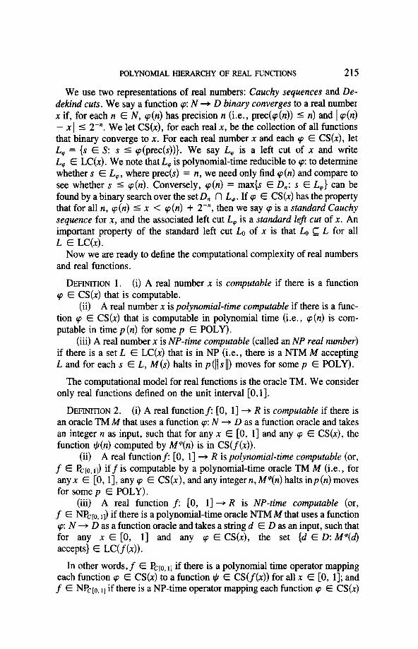
We use two representations of real numbers: Cauchy sequences and De- dekind cuts. We say a function q: N + D binary converges to a real number x if, for each n E N, q(n) has precision n (i.e., prec(cp(n)) 5 n) and 1 q(n) - x 1 I 2-“. We let CS(x), for each real x, be the collection of all functions that binary converge to x. For each real number x and each cp E CS(x), let L, = {s E S: s I cp(prec(s))}. We say L, is a left cut of x and write L, E LC(x). We note that L, is polynomial-time reducible to 90: to determine whether s E L,, where prec(s) = n, we need only find q(n) and compare to see whether s I cp (n). Conversely, q(n) = max{s E D,: s E Lrp} can be found by a binary search over the set D, n L,. If Q E CS(x) has the property that for all n, I 5 x < I + 2-“, then we say Q is a standard Cauchy sequence for x, and the associated left cut L, is a standard left cut of x. An important property of the standard left cut J~Q of x is that & C L for all L E LC(x).

Now we are ready to define the computational complexity of real numbers and real functions.

DEFINITION 1. (i) A real number x is computable if there is a function Q E CS(x) that is computable.

(ii) A real number x is polynomial-time computable if there is a function Q E CS(x) that is computable in polynomial time (i.e., I is computable in time p (n) for some p E POLY).

(iii) A real number x is NP-time computable (called an NP real number) if there is a set L E LC(x) that is in NP (i.e., there is a NTM M accepting L and for each s E L, M(s) halts in p (11 s 11) moves for some p E POLY).

The computational model for real functions is the oracle TM. We consider only real functions defined on the unit interval [O,l].

DEFINITION 2. (i) A real functionf: [0, l] + R is computable if there is an oracle TM M that uses a function Q: N -+ D as a function oracle and takes an integer n as input, such that for any x E [0, l] and any Q E CS(x), the function $(n) computed by M+‘(n) is in CS(f(x)).

(ii) A real functionf: [0, l] + R is polynomial-time computable (or, f E PclO, ,I) if f is computable by a polynomial-time oracle TM it4 (i.e., for anyx E [0, 11, any Q E CS(x), and any integer n, MQ(n) halts inp(n) moves for some p E POLY).

(iii) A real function f: [0, l] + R is NP-time computable (or, f E NPclo, 1J if there is a polynomial-time oracle NTM M that uses a function Q: N + D as a function oracle and takes a string d E D as an input, such that for any xE[O, l] and any Q E CS(x), the set {d E D: M’(d) accepts} E LC(f(x)).

In other words, f E Pcro, 1l if there is a polynomial time operator mapping each function Q E CS(x) to a function JI E CS(f (x)) for all x E [0, 11; and f E NP,L~, ,I if there is a NP-time operator mapping each function Q E CS(x)

216 KER-I KO

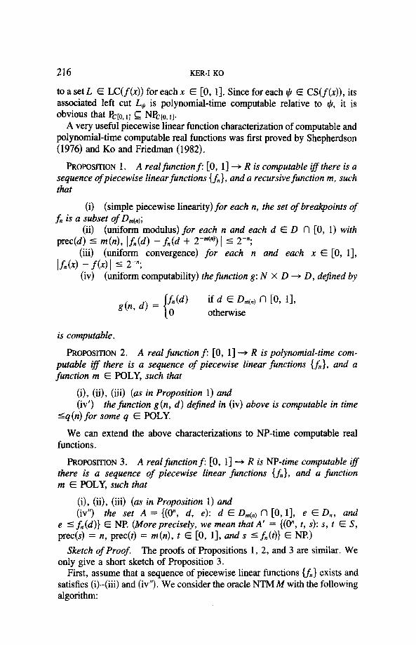
to a set L E LC(f(x)) f or each x E [0, 11. Since for each (I/ E CS(f(x)), its associated left cut L, is polynomial-time computable relative to @, it is obvious that Pcro, 1~ G NPc[,-,, l~.

A very useful piecewise linear function characterization of computable and polynomial-time computable real functions was first proved by Shepherdson (1976) and Ko and Friedman (1982).

hOPOSITION 1. A realfunctionf: [0, l] -+ R is computable ifs there is a sequence of piecewise linearfunctions { fn}, and a recursivefunction m, such that

(i) (simple piecewise linearity) for each n, the set of breakpoints of fn is a subset of D,(,);

(ii) (uniform modulus) for each n and each d E D f~ [0, 1) with prec(d) I m(n), 1 fn (d) - fn (d + 2-“‘“‘) ( 5 2-7

(iii) (uniform convergence) for each n and each x E [0, 11, If”(x) - f 64 I 5 2-7

(iv) (uniform computability) the function g: N X D + D, defined by

gh 4 = if d E D,(,) n [O, 11, otherwise

is computable.

~OPOSmON 2. A real function f: [0, l] + R is polynomial-time com-

putable ifs* there is a sequence of piecewise linear junctions {fn}, and a function m E POLY, such that

(i), (ii), (iii) (as in Proposition 1) and (iv’) the function g(n, d) defined in (iv) above is computable in time

<q(n) for some q E POLY.

We can extend the above characterizations to NP-time computable real functions.

PROPOSITION 3. A real function f: [0, l] --, R is NP-time computable iff there is a sequence of piecewise linear functions {fn}, and a function m E POLY, such thut

(i), (ii), (iii) (as in Proposition 1) and (iv”) the set A = {(W, d, e): d E D,(,) f~ [O,l], e E D,, and

e I fn(d)} E NP (More precisely, we mean that A’ = {(O”, t, s): s, t E S, prec(s) = n, prec(t) = m(n), t E [0, 11, and s I fn(t)} E NP.)

Sketch of Proof. The proofs of Propositions 1, 2, and 3 are similar. We only give a short sketch of Proposition 3.

First, assume that a sequence of piecewise linear functions cfn} exists and satisfies (i)-(iii) and (iv”). We consider the oracle NTM M with the following algorithm:

POLYNOMIAL HIERARCHY OFREAL FUNCTIONS 217

With oracle cp and input e E D, , M queries oracle to get d = ~(m (n + 2)) and accepts e iff (On+2, d, e - 2-(“+I)) E A.

By conditions (ii) and (iii), we know that If(x) - fn+2(d) 1 % 2-(‘+‘) if cp E CS(x). Since M’ accepts e iff e - 2-(“+I) ~f~+~(d), we have le’ -f(x)1 5 2-“, wheree’ = max{e E D,: MQ accepts e}. Thus {e E D: MQ accepts e} E LC(f(x)).

Conversely, assume that M is a polynomial-time oracle NTM such that MQ accepts a left cutf(x) whenever p E CS(x). Let t E POLY be a time bound for M and let m(n) = t(n + 1). Then m satisfies the following condition:

Ix - y I 5 2-“(“) implies If(x) - f(y) I 5 2~(“+I). (*I

For each d E D,(,) n [0, 11, let cp be the standard Cauchy sequence for d. Definef,(d) = max{e E D,: MQ accepts e}. Then it is clear that {fn} and m satisfy conditions (i)-(iii) and (iv”). n

The condition (*) in the above proof is an important property of functions in Pc[a,l~ and NPcIo,il. It is shown in Ko and Friedman (1982) that a real functionf has a polynomifally bounded modulus function m (i.e., f satisfies condition (*) with m E POLY) iff f is polynomial-time computable relative to an oracle set E.

Two-dimensional polynomial-time computable real functions are similarly defined. Namely, a real function f: [0, 11’ + R is in Pc[o,1~2 if there is a polynomial-time oracle TM M which uses two oracle functions cp and +;such that the function e(n) = MQ’,*(n) binary converges tof(x, y) if ‘p E CS(x) and J, E CS( y). The proof of the following proposition is similar to the one-dimensional case and is omitted.

PROFQSITION 4. A realfunction f: [0, 11” + R is in Pcla, Il2 iSfthere is a sequence of piecewise linear functions {f.} on [0, 112, and a function m E POLY, such that

(i) for each n, the breakpoints offn are {(d, e): d, e E D,(,) fl WY 1119

(ii) for each n and each d, e E D,(,, fl [0, l]

Ifn(d, e) - fn(d, e + 2-“9 I % 2-” if e # 1.0,

(f,,(d, e) -fn(d + 2-“(“‘, e)l s 2-” if d # 1.0,

(iii) for each n and x, y E [0, 11,

Ifnk Y) - fb, Y) 1 5 2-“,

U?d

(iv) the function g, dejined by

218 KER-I KO

g W, 4 4 = fn@, 4 if 4 e E &(,) n [O, 11, = 0 otherwise,

is polynomial-time computable.

3. MAXIMIZATION ON REALFUNCTIONS .

In this section we consider the maximization problem on real functions. Our main result is the characterization of the computational complexity of the maximization problem by the concept of NP-time computable real functions.

We first recall that for computable real functions, the maximum value y = max{f(x): x E [0, l]} of a computable real function f must be computable; on the other hand, Specker (1959) showed that there exists a computable real function f on [0, l] that does not take its maximum at any computable real number. At the polynomial-time level, the set of maximum values of polynomial-time computable real functions are not known to be polynomial-time computable. The best we can say about their complexity is that they constitute the set of all NP real numbers.

THEOREM 5. (Ko , 1982). A real number x is NP-time computable &f there is a function g E Pc[,,, ,I such that x = max(g( y): y E [0, 11).

Sketch ofProof. Since the proofs of Theorems 6 and 7 are similar to but more complicated than this proof, we reprove this result first. Our proof here uses Propositions 2 and 3 and is simpler than the original one.

First, the “if” direction is straightforward, following from the existential quantifier characterization of the class NI? We will show only the “only if’ direction.

Assume that L is a left cut of x and L is in NP (We emphasize that L is a set of strings in S = { + , -}{O, l}* * (0, 1)” with the property that if prec(d) = prec(e) and d 5 e then e E L implies d E L). We also assume, without loss of generality, that i I x 5 i. By the existential quantifier characterization of the class NP, there exist a polynomial-time predicate R, and a functionp E POLY, such that for all d E D tl [0, 11, if d = 0 * t for some t E (0, l}*, then

dEL iff (% 11 s II = p (II t ll>M (t, 4.

(Note that for each string t E (0, l)*, we write 0. t to denote the dyadic rational whose binary representation is 0 * t.) We assume that p(n) >p(n - 1) foralln 2 1.

We will construct a sequence of linear piecewise functions (g,} on [0, l] with the following properties:


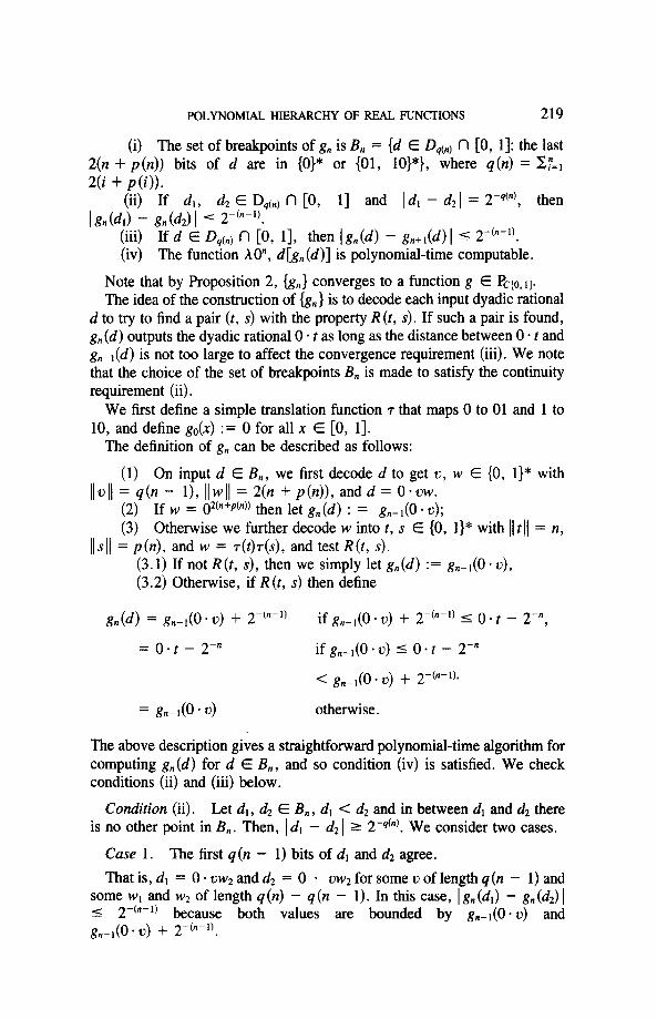
(i) The set of breakpoints of g, is B, = {d E DsCnj n [0, 11: the last 2(n + p(n)) bits of d are in {0}* or (01, lo}*}, where q(n) = Zy=, 2(i + p(i)).

(ii) If d,, d2 E DqCn) tl [0, l] and 1 d, - d2 1 = 2-q(nJ, then 1 g,(4) - g,(4) 1 5 2-(“-‘).

(iii) If d E DqCnj rl [0, 11, then jgn(d) - g,+l(d) 1 I 2-(“-l). (iv) The function ho”, d[g,,(d)] is polynomial-time computable.

Note that by Proposition 2, {g,} converges to a function g E Pcto, ,I. The idea of the construction of {g,} is to decode each input dyadic rational

d to try to find a pair (t, S) with the property R(t, s). If such a pair is found, g,(d) outputs the dyadic rational 0 * t as long as the distance between 0 * t and gn-,(d) is not too large to affect the convergence requirement (iii). We note that the choice of the set of breakpoints B, is made to satisfy the continuity requirement (ii).

We first define a simple translation function T that maps 0 to 01 and 1 to 10, and define go(x) := 0 for all x E [0, 11.

The definition of g, can be described as follows:

(1) On input d E B,, we first decode d to get u, w E (0, 1)” with )IbII = q(n - l), IIwII = 2(n + p(n)), and d = 0.0~.

(2) If w = 02(n+J’(“)) then let g,(d) : = g,-,(O . u); (3) Otherwise we further decode w into t, s E (0, l}* with II t II = n,

IIsI] = p(n), and w = T(t)+), and test R(t, s). (3.1) If not R(t, s), then we simply let g,(d) := g,-l(O.u), (3.2) Otherwise, if R(t, s) then define

g,(d) = g,-,(O*v) + 2-(“-l) if g,-,(O . u) + 2-(“-‘) I 0. t - 2-” 9 = 0. t - 2-n if g,-,(O . u) 5 0 * t - 2-”

< g,-,(O * u) + 2-c”-‘),

= &I@ * 4 otherwise.

The above description gives a straightforward polynomial-time algorithm for computing g,(d) for d E B,, and so condition (iv) is satisfied. We check conditions (ii) and (iii) below.

Condition (ii). Let dl, d2 E B,, d, < d2 and in between dl and d2 there is no other point in B,. Then, I d, - d2 I 2 2-q(“). We consider two cases.

Case 1. The first q (n - 1) bits of dl and d2 agree.

Thatis,d, = 0.uw2andd2 = 0 . 2)w2 for some u of length q(n - 1) and some w1 and w2 of length q(n) - q (n - 1). In this case, I g, (d,) - g, (d2) 1 5 2-(“-‘) because both values are bounded by g,-i(O * u) and g,-,(O * u) + 2-+-l).

220 KER-I KO

Case 2. Not Case 1. Then, it must be the case that d, = 0. ulwl and d2 = 0.t~~~~~ where

0 - *2 = 0. q + 2-q(n-‘), q = (l())n+Pb), and w2 = 02(“+p(n)). By induction, lgn-do - 01) - gn-,(O * 02) 1 5 2-(n-2). So, (g,(d,) - g,(dJ 1 5 2-(n-3), because g, (4) = g,-I(0 - ~2) and 1 g, (dl) - g,-,(O * q) 1 C= 2-(“-‘). Note that the distance between dl and d2, in this case, is at least 2-(q(“-‘)+2). So, for any d3 and d4 with distance 2-4cn), 1 g, (dJ - g, (d,J I 5 2-‘“-3’2-2 5 2-(“-l), since we assumed that p(n) > p(n - 1).

Condition (iii). Note that if d = 0. IIW with (I 2) I( = q(n - 1) and ]lwl] = q(n) then g,-1(O-u) 5 g.(d) 5 g,-i(0.u) + 2-(“-l). So, by condition (ii) above, 1 g,+(d) - g,(d) I 5 2-(n-2).

Finally we check that max{g ( y) : y E [O, l]} = x. Let cp be the standard Cauchysequenceforx.Then,foreachn 2 l,cp(n)=O~r,, sx <O-t,+ 2-“, for some 6, E (0, l}* and 0. cn E L. (Recall that the standard left cut of x is contained in every left cut of x.) So, there exists, for each n, an s, such that IIs,, II = p(n) and R(t,, s,). Let d,, = 0. T(~,)T(s,) . * * T(z,,)T(s,,). Then g,(d,) = 0 + t,, - 2-” because by induction 0 * tn- 1 - 2-(“-l) = g,- ,(d,- J and so g,-,(d,-J + 2-(“-l) = 0. tnwi 2 0. t,, - 2-“. So, g(lim,.&) = x, and max{g(y): y E [0, l]} 2 x.

Conversely, we can easily show, by induction, that g,,(d) 5 0 * t, for all d E B,. So, max{g(y): y E [O.l]} 5 x and the proof is complete. n

The above theorem characterizes the set of maximum values of real functions as the set of NP real numbers. However, the exact relation between the complexity of NP real numbers and the P = ?NP question is still not clear. We discuss this question in Section 5. The next theorem generalizes Theorem 5 to two-dimensional real functions and gives a characterization of NP-time computable real functions. It also generalizes Friedman’s (1984) result that the maximum problem of a polynomial-time computable two-dimensional real function is always solvable in polynomial time iff P = NP.

Since we are concerned with computable, continuous functions with domain [0, 1, we will assume, for the sake of simplicity, that the ranges of these functions are contained in [0, 1. Also, in the rest of the paper, we write D and D, to denote D rl [0, l] and 0, fl [0, 11, respectively.

THEOREM 6. A realfunctionf: [0, l] + [0, l] is NP-time computable if there is a polynomial-time computable realfunction g: [0, 112 + [0, l] such thatfor all x E [0, 11, f(x) = max{g(x, y): y E [0, 11).

Proof. (rf) Assume that A4 is a (two-)oracle TM computing g in timep (n) for some p E POLY. Then we can define a sequence of piecewise linear functions {fn} as follows.

For each n, the set of breakpoints of fn is exactly Dp(n+9. For each d E Dp(n+2Jr define fn(d) to be max {Md3e(n + 2): e E D,++2~}, where


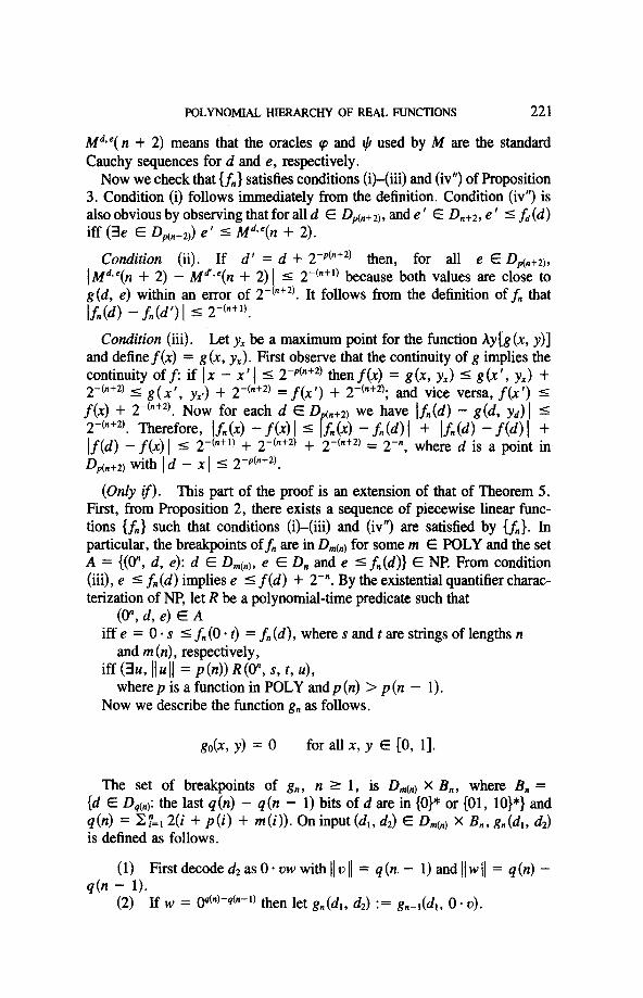
WQ( n + 2) means that the oracles cp and I++ used by it4 are the standard Cauchy sequences for d and e, respectively.

Now we check that (fn} satisfies conditions (i)-(iii) and (iv”) of Proposition 3. Condition (i) follows immediately from the definition. Condition (iv”) is also obvious by observing that for all d E Dp(n+Z), and e ’ E D,,+*, e ’ 5 fd (d) iff (3e E Dp(n+a)) e ’ 5 Mdsc(n + 2).

Condition (ii). If d’ = d + 2-P(“+2) then, for all e E Ddn+2), IMd*e(n + 2) - Md’-‘(n + 2) 1 5 2- WI) because both values are close to g(d, e) within an error of 2- (n+2). It follows from the definition of fn that j&(d) - fn(d’) 1 5 2-(“+l).

Condition (iii). Let yX be a maximum point for the function Ay [s (x, y)] and define f(x) = g (x, y*). First observe that the continuity of g implies the continuity of f: if I n - x ’ 1 I 2-p(n+2) then f(x) = g (x, yX) I g (x ’ , yJ + 2-(n+2) I g (x ‘, yxr) + 2-(n+2) = f(x ‘) + 2-(n+2); and vice versa, f(x ‘) 5 f(x) + 2-(“+2). Now for each d E D (“+z) we have If”(d) - g(d, yd) I 5 T(~+~). Therefore, If.(x) - f(n) 1 5 pf.0 - fn@) I + Ifn(4 - f(d) I + If(d) - f(x) I 5 2-(“+r) + 2-(n+2) + 2-(“+2) = 2-“, where d is a point in Dp(n+2) with Id - xl I 2-p(n+2).

(Only if). This part of the proof is an extension of that of Theorem 5. First, from Proposition 2, there exists a sequence of piecewise linear functions {fn) such that conditions (i)-(iii) and (iv”) are satisfied by {fn}. In particular, the breakpoints offn are in D,(,) for some m E POLY and the set A = {(p, 4 4: d E D,(,,,, e E D, and e I fn(d)} E NI! From condition (iii), e <f”(d) ’ pl im ies e I f(d) + 2-*. By the existential quantifier characterization of NP, let R be a polynomial-time predicate such that

(0”, d, e) E A iff e = 0 . s 5 fn (0 * t) = fn (d), where s and I are strings of lengths n

and m (n) , respectively, iff (3~ II~II = p(n)) R@“, s, t, 4,

where p is a function in POLY andp(n) > p(n - 1). Now we describe the function g, as follows.

gob, y) = 0 for all x, y E [0, 11.

The set of breakpoints of g,, n L 1, is D,,,(,) X B,, where B, = {d E D& the last 4 (n) - q(n - 1) bits of d are in {0}* or (01, lo}*} and q(n) = x7=‘=12(i + p(i) + m(i)). On input (d,, d2) E D,(,, x B,, gn(dl, d2) is defined as follows.

(1) First decode d2 as 0 * uw with ]I u 1) = q(n. - 1) and 11 w /I = q(n) - q(n - 1).

(2) If w = Oq(n)-q(n-l) then let g,(d,, d2) := g,-l(dl, 0. u).

222 KER-I KO

(3) Otherwise we decode w = T(t)T(u)T(s) with IIs I] = n, [[t/l = m(n), and I]uj] = p(n) and test R(O”, s, t, u).

(3.1) If not R(O”, s, t, u) then let g,(d,, d2) := g,-i(di, 0.~). (3.2)Otherwise,computee’: = 0~s - Id, - O.t/2”(+” - 2+-‘),

and let

g n (dl, d2) = g,-,(dl, 0 *u) + 2-(n-4) if g _ I(d, 0 -0) + 2+-4) 5 e ’ , n 7 = e’ if g,-l(d,, 0.~) 5 e’

< g,-l(d,, 0 * u) + 2-(n-4),

= gn-d4, 0 * 4 otherwise.

We note that the definition of g, is similar to that of g, in the proof of Theorem 5, and we need to verify that {g,} satisfies the conditions (i)-(iv) of Proposition 4. We note that conditions (i) and (iii) and the first inequality of (ii) can be proved similarly to that of the proof of Theorem 5, because for each fixed x, the function hy [g, (x, y)] is essentially the same as g, defined in Theorem 5.

Condition (ii). We need to verify the second inequality of (ii). In other words, if 4,d2 E Q,), 4 E Dqcn), and d2 = dl + 2-“‘“), then I g, (d,, d3) - g,(d*, d3) ( s 2-(n-3). The main idea here is that in step (3.2) of the definition of &I, when we decode d3 and find witness u for the relation [0 . s 5 &(O*t)],ifO.t = d,th en we make g, (d, , d3) = 0 . s - 2-(“-l) to make max g, at dl close tofn (d,), and even if 0. t = d2 # d,, we still make the value of g,(d,, d3) as close to 0. s - 2-(“-‘) as possible to satisfy the continuity requirement for g.

More precisely, we assume, without loss of generality, that m(n) > m (n - 1) + 1, and also assume, by induction, that I g,-,(d,, d3) - g,-,(dz, d3) 1 I 2-(“-4)2-2 = 2-(n-2). (Note that Id, - d2 I I 2-22-“‘“-1’.) Now, decode d3 = 0. z)w with 11 o ]I = q(n - 1) and I] w I] = q(n) - sb - 1).

If [w = (-yWdn-1) ] or [w = T(t)T(u)T(s) and not R(O”, s, t, u)] then g,(dl, dJ = g,-d4, 0.0) and g,(& 4 = gn-dd2, O-u>, and so Ig,(4, 4 - g,(d2, d,) 1 I 2-(n-2)

Otherwise (i.e., i (0”, S, t, u)), then 1 10. t - dl I - IO * t - d2 I ( = ld,yn$~~cn2;m(fnl. So, Je; - eil = 2-“, where e[ ==C).S - 10.: - dtl .

, or i = 1, 2. It follows from the definmon and the mductive hypothesis that I g,(dl, d3) - g,(& 4) I 5 I g,-l(4, 0 * 4 - gn-l(d2, 0 * 0) I + le; - e;l 5 2-(n-2) + 2-n 5 2-(n-3).

Condition (iv). Following the definition of g,, we have the following algorithm for computing g,(dl, d2) with dl E &(,I and d2 E D4(,,):

First let lower(dJ := max{d E B,; d 5 d2},


upper(&) := min(d E B,: d 1 dz}, left@,) := max{d E D,,+r): d I dl}, right(dJ := min{d E D,,+,): d L d,}, leftlow := max{d E Dq+r): d I lower(dz)}, leftup := max{d E Ds(,,-r): d 5 upper(dJ},

and let rl and r2 be dyadic rationals in [0, l] such that dl = (1 - r,) * left(dJ + rl . right(dJ and d2 = (1 - r2) * lower(d2) + r2 . upper(d2).

(Note that it is possible that left(d,) = right(dJ, and in this case we let r1 := 0. The same rule applies for r2.)

Next define e1 := g,-,(left(dJ, leftlow(d e2 : = g,-,(left(d,), leftup(d e3 := g,-r(right(d,), leftlow(d2)), e4 := ,g,-,(right(dJ, leftup(d2)).

Then we have e5 := g,-,(dl, leftlow(d2)) = (1 - r,). el + rl - e3, and e6 := g,-,(d,, leftup(d2)) = (1 - rl)*e2 + rl-e4.

Following the definition of g,, we can compute, using e5 and e6, e7 : = g, (d,, lower(d2)) and e.3 : = g, (4, upper(

Finally, we get g,@l, 4) := (1 - r2l.e + r2 ’ eg.

We note that in the above algorithm we made four recursive calls to the algorithm itself for the values el, e2, e3, and e4. (Note that left(d,) and right(dr) are in D ,,,tn-,) and leftlow and leftup(dJ are in Dq(,,-+) Therefore, if the algorithm is called recursively, then we would have to make 4”-’ many calls to reach the trivial case of evaluating go, and this would give an exponential-time algorithm. To avoid this problem, we can use the concept of dynamic programming to actually call gn-2(dl, dz), with dl E Drncnm2) and d2 E D,+2), only four times. To see this, we observe that for any dl E D,(,,, left(left(dl)) = left(right(d,)), right(left(dJ) = right(right(dJ), and for any 4 E Dq(n), leftlow(leftlow(d2)) = leftlow(leftup(d2)) and leftup(leftlow(d2)) = leftup(leftup(d2)). Therefore we can use a bottom-up algorithm to compute gi (lefti @J, lefilowi (dz)) , gi (lefti Cd,), leftpi (4)) , gi (fighti (dl) 3 lefilowi (4)) and gi (@hti (dd 3 leftupi (4)) f or i : = 0 to n, where left, (d,) is defined to be max{d E Dm(i): d 5 d,}, ad righti (dJ, leftlowi(d2) and leftttpi(d2) are similarly defined. This proves the polynomial-time computability of the function AO”, 4, ddg, (4, 41.

Finally we need to check that for each x, f(x) = max{g (x, y): y E [0, 11). For each x E [0, 11, let X, be the maximum dyadic rational in D,(,, that is I x, and x,’ = x, + 2-m(“). We note that for each rr, ]fn(xn) - f(x) 1 I

224 KER-I KO

2-(“-r). We claim that for each n E N and d E B,, g,(x,,, d) 5 f(x) and &I b,’ 9 4 5 f(x).

We prove this claim by induction on n. First, if g,, (x, , d) = g,-l(x,, 0 * u), where u is the first q(n - 1) bits of d,

then, by the inductive hypothesis and the piecewise linearity of g,,-1, g,(x,, 4 5 m=&-dx,-l, d)gn-dXi-t, 41 <f(X).

Otherwise, if g,(x,, d) > gnFl(xn, 0 * u), then when we decode d into 0 - UT(~)T(U)T(S) we have R(O”, s, t, u) and g,(x,,, d) I e’ = 0 es - Ixn _ 0. tl .pW-~ _ 2-h-1). s ince fn has a modulus of continuity m (n) and since fn is piecewise linear, we have Ifn(.%> -h(O*t)I 5 2yxn - 0+2”‘“‘. so, g,(x,, 4 5 0-s - Ihbn) -fn(WI - 2+-l) sf.(O*t) - Ifn(xn) -fn(O* t)l - 2+-l) Ifn(xn) - 2-c”-‘) 5 f(x). g,(x,’ , d) 5 f(x) can be proved similarly.

Therefore, wehave, foreveryx,y E [0, l],g(x,y) = lim,,g,(x,,, y) 5 f (4.

Next, consider d,, = 0. ~(x,)T(t,)~(fi(x,)) * . . T(xn)T(tn)T(fn(x,)), and claim that g (x d ) 2 fn(xn) - 2-(“-‘).

Assume, iy %dktion, that gn-,(xn-,, d,-,) 2 fnml(xnel) - 2-(n-2). Then, g,-,(x,,, d,-1) zr fnJxn-,) - 2-(“-3) - 2-(n-2) (by the second part of condition (ii) of {g,}) and 2 f”(x,J - 2-(“-l) - 2-(n-4) (by the continuity and convergence of {f”}). Furthermore, the value e ’ evaluated in step (3.2) of the definition of g, is equal to fn (xn) - 2-(“-‘). So, from the definition of g, (step (3.2)), gnk9 4) zfn(xn) - 2- - cn ‘). From the claim, we have g(x, Iim,Jw)=Iim,, g,, (xn , d,, ) 2 x. This completes the proof of Theorem 6. n

4. A POLYNOMIAL HIERARCHY OF REAL FUNCTIONS

In Section 3, we gave a characterization of NP-time computable real functions in terms of the maximization operation. We note that the proof technique of this characterization relativizes; that is, we can actually prove that, for any set E, f is NP-time computable on [0, l] relative to E iff there is a function g that is polynomial time computable on [0, 11’ relative to E, such thatf (x) = max{g(x, y): y E [0, 11). This suggests that we may extend the class of NP-time computable real functions to a polynomial hierarchy and provide a natural characterization for this hierarchy by the alternating operations of maximization and minimization. We discuss this idea in this section.

First we define the polynomial hierarchy of real functions. It is natural to define Z g,c[,,, ,I, k 2 1, to be the class of real functions f on [0, l] that is computable by a polynomial-time two-oracle NTM M with respect to an oracle B E Xc--,, in the sense that M uses B and a function rp E CS(x) as oracles and the set {d E D: MQ,B accepts d} E LC( f (x)). It is straightforward to relativize Proposition 3 to get the following equivalent definition. We use the following definition because it is more useful in proving the characterization results.

POLYNOMIAL HIERARCHY OFREAL FUNCTIONS 225

DEFINITION 3. For k 2 0, we say a real functionf: [0, l] + [0, l] is in X~,c[,-,l] (II~,c[O,l], A~,c[,,J if there exists a sequence of piecewise linear functions {fn}, and a function m E POLY, such that

(i), (ii), and (iii) of Proposition 1 hold, and (iv) the set A = {(0”, d, e): d E D,(,), e E D,, and e I f”(d)} E

C P(IIP, A!, respectively).

Using this definition, we generalize Theorem 6 to the following:

THEOREM 7. Let k L 0. A realfinctionf: [0, l] -+ [0, l] is in 2 Rl,c[o, 11 #there is a real function g: [0, 11’ + [0, l] that is in IIF,cp,, 1~z such thatfor all x E [O, l],f(x) = mdg(x, Y): Y E P, 111.

Proof. The proof is almost the same as that of Theorem 6. First, f E Z;+l,c[O,ll implies that 0-s Ifn(O-t) iff (5, I/u]] = p(n))

R (o”, S, t, u) , for some II: -predicate R. Now define (g,} exactly the same as that in the proof of Theorem 6. Then, it follows from the same proof that (g,} satisfies (i)-(iii) of Proposition 4 and (g,} converges to some function g such that for all x, f(x) = max{f(x, y): y E [0, 11). The only thing left to show is that the set B = {(0”, e, d,, d2): e E D,, d, E D,,,(,,, d2 E Dd,,), and e I g,(d,, d2)} E IIF. (The proof of Theorem 6 gave B E Ai+r .) We will use the notation defined in the proof of Theorem 6.

From the definition of g,, to compute g,, (d,, d3), with d, E D,,,(,J and d3 E B, , it involves the decoding of d3 to extract the strings S, t, u, and u and the dyadic rational e ’ . This decoding process takes only a polynomially bounded amount of time. Using these values we can simplify the predicate [e 5 g,(d,, dJ] with e E D,, d, E D,(,,,, and d3 E B,, as follows: (Note that leftlow(dJ = leftup = 0. u, because d3 E B,.)

e 5 g,(4, 4 iff [e 5 g,-,(dl, leftlow(d or [R(O”, s, t, u) and e 5 e’ and e -

2-(n-4) I g,-,(d,, leftlow(dJ because g,(dl, d3) > g,-,(d,, leftlow( implies g,(d,, dJ = min{e ‘, g,- l(dI, leftlow(d3)) + 2-(“-4)}.

The predicate [e I g,-,(d,, d;)], with d, E D,,,) and d; E D,(,-,) can be further simplified as follows:

e 5 g,-d4, 4) iff VelVed [el > g,-&Wd, 6) and e2 > g.-~~~ght(dA 411 3

e 52 (1 - rr)er + rre2] iff VelVe2[el I g. _ ,(left(d,), d;) or e2 d g,,-r(right(d,), di) or e I

(1 - $3 + w21.

Together, we have

e s g&l, 4) iff verb[er 5 g,,-r(left(dr), leftlow( or e2 Ig,-r(right(d,), leftlow(d3))

226 KER-I KO

or e I (1 - r&i + rle2 or [R(O”, S, t, u) and e I e’ and e - 2-(n-4) d (1 - rJei + rle2] 1. (1)

Now consider [e 5 g,(d,, d,)], with e E D,, dl E D,(,,, and d2 E D4(,+ We have

iff Ve-rVeg [e7 I g, (d,, lower(d2)) or e8 5 g,(d,, upper(d2)) or e 5 (1 - r2k7 + r2e81. (2)

Combining (1) and (2), we can reduce [e I g,(d,, d2)] to a predicate of the following form:

e 5 g,(4, 4) e 5 g,(4, 4) iff VelVe2Ve3Ve4 [el I g,-l(left(d,), leftlow( or e2 sg,-i(right(dJ, iff VelVe2Ve3Ve4 [el I g,-l(left(d,), leftlow( or e2 sg,-i(right(dJ,

leftlow(d2)) or e3 5 g,-,(left(dl) leftup(d2)) or e4 I g,-,(right(dJ, leftlow(d2)) or e3 5 g,-,(left(dl) leftup(d2)) or e4 I g,-,(right(dJ, leftqd4)) or Sk, e2, e3, e4, 41 leftqd4)) or Sk, e2, e3, e4, 41 (3) (3)

where S(el, e2, e3, e4, e) is a predicate of the form

Ve7Ve8 [A, or A2 or A3 or [Z?, and A4] or [R2 and As] ]

and Ai’S are polynomial-time predicates and Rj’S are II:-predicates, i = 1, . . . 7 5andj= 1,2.

When we simplify (3) recursively, we need, at each step, only to introduce four more universal quantifiers and four more S-type predicates, because of the relations such as left(left(dl)) = left(right(d,)), as discussed in the proof of condition (iv) in Theorem 6.

iff Vel - + * Ve4Ve; - - * Ve;[Ql or * * * or Q4 or S1 or . * * or S4 or S],

where Qi is of the type ei’ 5 g,-z(dy, di) with dy E Dm(n-2) and di E Dqcn-2~, i = 1, 2, 3, 4; and Si = S(e;, el, ei, ei, ei), i = 1, 2, 3, 4; and S = Sk, e2, e3, e4, e).

A complete expansion will then produce a predicate of 4n universal quantifiers followed by 4n - 3 S-type predicates. Since each S-type predicate contains two universal quantifiers and two occurrences of R-type predicates, it shows that the predicate [e 5 g, (dl, d2)] is in II,‘, and this completes the proof. n

The proofs of Theorems 6 and 7 can also be generalized to multi- dimensional functions. In other words, a real functionf: [0, 11” + [0, 11, for some I?z 2 1, is in S[++I,c[O, I]” ifff(xr, . . . , xm) = max{g(x,, . . . , x,, y): y E [0, l]}for someg E II:,c[O,llm+l. (The only difference in proof from that of Theorem 7 is that when the function g, is constructed, we need to make it to be continuous in all m + 1 variables. This is easy to handle using the technique used in step (3.2) of the definition of g,, in Theorem 6.) Thus, we have the following corollary.

POLYNOMIALHIERARCHYOFREALFUNCTIONS 227

COROLLARY 8. Let k 2 1. A realfinctionf [0, l] + [0, l] is in ZE,c[,, l~ if there is a function g E Pc[O,l~+~ such thutfor all x E [0, 11,

where optk = max if k is odd (= min if k is even).

5. STRUCTURE OF THE POLYNOMIAL HIERARCHY OF REAL FUNCTIONS

In Section 4, we defined a polynomial hierarchy of real functions and showed a natural correspondence between this hierarchy and the operations of maximization and minimization. In this section we study the structure of this hierarchy. In particular, we ask whether the hierarchy is an infinite hierarchy. The answer is that for every k 2 1, 2: = IIF iff ~,!,c[o, i] = I&[o,II; ad P = NP iff PC[O,II = W[O,II.

First we note that the following theorem follows immediately from Definition 3.

THEOREM 9. For each k L 1, 2: = II,’ implies C&JI = I’IF,~c~,~J

We recall that Baker, Gill, and Solovay (1975) and Baker and Selman (1979) have shown that the polynomial hierarchy of operators extends at least two levels. Thus, Theorem 9 shows that the polynomial hierarchy of real functions is different from the polynomial hierarchy of operators. We note that the difference lies on the inherent structure of real numbers. In the following we illustrate, in general, how the structure of left cuts affects the oracle computation when they are used as oracles. In particular, we show that a left cut, when used as an oracle, cannot distinguish NP-operators from P-operators, unless P # NP To begin with, we review some definitions.

DEFINITION 4. (Karp and Lipton, 1980). A set A c (0, l}* has polynomial-size circuits, or A E P/poly, if there are a polynomial length-bounded function h: {0}* + (0, l}* and a set B E P, such that for each s E (0, l}*,

s E A iff (s, h(O1lsll)) E B.

Meyer has shown that A E P/poly iff there is a sparse set S such that A E Ps (Berman and Hartmanis, 1977). (A set S C (0, l}* is sparse if there is a function p E PGLY such that for every n, the size of the set {s E S: ]I s I] = n} is bounded by p(n).) Karp and Lipton (1980) and Sipser showed that a set A in P/poly cannot be NP-complete unless Z p = II;. Ko (1983) showed that a left cut of a real number is in P/poly . In the following, we give a stronger result.

DEFINITION 5. A set A C (0, l}* has self;producible (polynomial-size) circuits if A E P/poly and the function h in Definition 4 is in PA.

228 KER-I KO

In other words, A has self-producible circuits if the circuits h(0”) that help the computation of “s E A” for those s with (1 s I( = n can be computed from A itself. It is easy to show that a left cut L of a real number has self-producible circuits.

LEMMA 10. (a) Zf A is a tally language (i.e., A C {O}*), then A has self-producible circuits.

(b) If L is a left cut of a real number, then L has self-producible circuits.

Proof. (a) Define h(0”) = 1 if 0” E A, and = 0 if 0” 4 A, and let B = {(o”, 1): n L 1) (cf. Long and Selman, 1983).

(b) Define h(V) = max{d E D,: d E L}, and B = {(e, d): prec(e) = prec(d) and e I d}. Note that h can be computed from L by a binary search, because a left cut L has the property that

be44 = P ret e , e I d and d E L] implies e E L. ( > n

Now, our result follows from Long and Selman’s (1983) observation that a set having self-producible circuits cannot distinguish NP-operators from P-operators.

THEOREM 11. (Long and Selman, 1983). For all k 2 1, Z [ = I’IIp implies ZF” = III,‘sA for all A that have self-producible circuits.

Sketch of Proof. The main observation is that B E Xc,‘,” iff there is a polynomial length-bounded function h: {0}* --, (0, l}*, and a set C E 2 E, such that for all s E (0, l}*, s E B iff (s, h(O11’ll)) E C. Furthermore, if A has self-producible circuits then h E PA. This is because the oracle A can be replaced by circuits h without increasing the complexity of B.

Now, Z F = II[ implies that the set C in the above is also in II,‘, and hence B E IIF”, because h E PA. n

COROLLARY 12. Let L be a lef cut of a real number. Then, for k 2 1, Z 1 = III,’ implies Z FL = @J; and P = NP implies PL = NPL.

Conversely, we want to show that Z 1, c10, 1~ = IIF, C[O, 1~ implies Z k’ = II,‘. We first examine the simplest case.

THEOREM 13. Pclo,l~ = NPct,,, 1~ implies P = NP

Sketch of Proof. Friedman (1984) showed that for every set A E NP, there is a real function gA E P =lo, 1l2 such that the function f (x) = max(g(x, gloYl,, ro, 111 is in Pclo,il iff A E P. So, it follows from Theorem 6 that

= NPcro, i] implies P = NP We can also give a direct proof that is similar to but simpler than the proof of Theorem 6.

Let A E NP. We construct a function f E NPclo, i] that embeds the set A such thatf E Pc,, i] iff A E P Since A E NP, there exists a polynomial-time predicate R, and a function p E POLY, such that s E A iff (3, ]I t[I = p (]I s ll))R (s, t). We construct a sequence of piecewise linear functions {fn} as follows.


The breakpoints offn are dyadic rationals in B, = {d E Dh: d = 0. w for some u E (01, lo}* and w E {O}*}. Note that d E B, - B,-I means that d = 0 * u for some 23 E (01, lo}*.

We letfT(x) = x for all x E [0, 11. For n 2 1, we define f, on d E B, as follows:

(1) For all d E K-1, J,(d) = fn-Ad), (2) For all d E B, - B,-,, we decode d into 7(t) (where T is the

translation function such that r(0) = 01 and ~(1) = 10) and let

fn(d) = d + 2-(2n+1) ift E A, = d otherwise.

It is a routine check to show that {fn} satisfies conditions (ii) and (iii) of Proposition 3. The key points are that

(1) foranyd E Bk - Brml, wherek 5 n, wemusthaved s&(d) = h(d) I d + 2-(“+‘); and

(2) if d and e are in B, and there is no other point in B, between d and e and if d or e is in Bk for some k I n, then (d - e 1 L 2-(2k+23.

In addition, we can verify that {fn} satisfies condition (iv”) of Proposition 3. Let e E D2,,+, and d E B, - B,-,. Then,

iff [e 5 d] or [e 5 d + 2-(2n+1) and t E A].

Now,fore E Dh+,andd ED 2n, we may use the piecewise linearity of {fn} to reduce this predicate as we did in the proof of Theorem 7.

iff (gel E &+I) (3e2 E &+J [el 5 fn(dJ and e2 5 fn(d2) and e 5 (1 - r).el + r*e2],

where dl, d2 E B, and r E D tl [0, l] are polynomial-time computable from d. Thus, by a reduction similar to that in the proof of Theorem 7, we can show that the predicate [e 5 fn (d)] is in NP

Finally, it is clear that if f E Pcro, ,I, then, for each t E (0, l}* with I] t 11 = n, we can computef, (0 . T(t)) correct to within an error of 2-““+2) and determine whether t E A according to whetherf,(O * T(t)) > 0. T(t) or not. (Note that since both fn (0 * T(t)) and 0 * T(t) have alternating bits 0 and 1 in every two bits, we can determine whether they are equal or not by obtaining only an approximation value of fn (0 * T(t)).) This completes the proof. n

In the above proof, let us replace A E NP by any set A’ in I; E, for some k 2 1, and construct the function f according to A’. Then we have f E x i,c[O,l~. Now assume thatf E II~,ctO,,~. Then the predicate [e I fn(d)] is in II!, and for each t of length n, we have

230 KER-I KO

tEA ifffn(O * T(t)) = 0 + 7(t) + 2-(2n+1) iff 0 . 7(t) + 2-@+l) 5 fn(O * 7(t)).

So, f E III,,, I~ implies A E II i. This gives the following corollary.

COROLLARY 14. For each k 2 1, C &[O, rl = II&r,,, i] implies 2 [ = II,‘.

Theorem 9 and Corollary 14 showed that the polynomial hierarchy of real functions, similar to the Meyer-Stockmeyer polynomial hierarchy, may collapse to any level, while the polynomial hierarchy of operators is known to have at least two proper levels, This difference is caused by the convergence requirement of the Cauchy sequence representation of real numbers. Some other effects of this structural constraint of real numbers have been discussed in Ko (1982, 1983):

(a) A left cut L of a real number cannot be NP-m-complete unless P = NP; and it cannot be NP-T-complete unless 2; = II!.

(b) It is known that P = NP implies 6 = NPR, and & = N& implies EXP = NEXP, where & (NP,) is the class of real numbers computable in deterministic (nondeterministic, respectively) polynomial time, and EXP (NEXP) is the class of sets (of binary strings) acceptable in deterministic (nondeterministic, respectively) time O(2’“) for some constant c. It is not known, however, whether pk = NPR implies P = NP In fact, this question is equivalent to one of the major open questions in complexity theory.

The reader is referred to these papers for details.

6. CONCLUSION

We have demonstrated the close connection between maximization and nondeterminism, in both discrete complexity theory and continuous complexity theory. A polynomial hierarchy of real functions is constructed as a continuous analog of the Meyer-Stockmeyer poiynomial hierarchy. It was shown that the complexity of the alternating operations of maximization and minimization has a natural characterization by this hierarchy.

It should be pointed out, however, that our formulation of the problem is of an abstract form, while most practical problems are of more complex forms. Nevertheless, our results may give a general direction and, in some cases, may simplify the complexity analysis of the maximization problems. One example is that the computational complexity of the degrees of best approximation by polynomials can be characterized exactly to be NP real numbers. This result will be discussed in a subsequent paper.

In Section 5, we touched briefly upon the structure of real numbers and its effect on the complexity of real functions. This issue appears important both in the complexity theory of real computation and in the structural study of


discrete polynomial complexity theory. Ko (1984) discussed further the role a left cut construct plays in the structural studies of polynomial-time reduc- ibilities and of relativization. This direction of research provides another interesting aspect of the interconnections between discrete complexity theory and continuous complexity theory.

REFERENCES

BAKER, T., GILL, J., AND SOL~VAY, R. (1975), Relativizations of the P=?NP question, SIAM .I. Comput. 4, 431-442.

BAKER, T., AND SELMAN, A. (1979), A second step toward the polynomial hierarchy, Theoret. Comput. Sci. 8, 177-187.

BERMAN, L., AND HARTMANIS, J. (1977), On isomorphisms and density of NP and other complete sets, SlAh4 .I. Comput. 6, 305-322.

FRIEDMAN, H. (1984), On the computational complexity of maximization and integration, Adv. in Math. 53, 80-98.

GAREY, M., AND JOHNSON, D. (1979), “Computers and Intractability,” Freeman, San Fran- cisco.

HOFCROFT, J. AND ULLMAN, J. (1979), “Introduction to Automata Theory, Languages, and Computation,” Addison-Wesley, Reading, Mass.

JOHNSON, D. (1974), Approximation algorithms for combinatorial problems, J. Comput. System Sci. 9, 256-278.

KARP, R., AND LIPTON, R. (1980)) Some connections between nonuniform and uniform complexity classes, in “Proceedings, 12th ACM Symposium on Theory of Computing,” pp. 302-309.

Ko, K. (1982), The maximum value problem and NP real numbers, J. Comput. System Sci. 24, 15-35.

Ko, K. (1983), On self-reducibility and weak p-selectivity, J. Comput. System Sci. 26, 209-22 1.

Ko, K. (1984), Applying techniques of discrete complexity theory to numerical computation, in “Studies in Complexity Theory” (R. Book, Ed.), Pitman, London, in press.

Ko, K. (1985), On some natural complete operators, Theoret. Comput. Sci. 37, l-30. Ko, K. AND FRIEDMAN, H. (1982), Computational complexity of real functions, Theoret.

domput. Sci. 20, 323-352. LONG, T., AND SELMAN, A. (1983), Relativizing complexity classes with sparse oracles, J.

Assoc. Comput. Mach., in press. SHEPHERDSON, J. (1976), On the definition of computable functions of a real variable, Z Math.

Logik Grundlag. Math. 22, 391-402. SPECKER, E. (1959), Der Satz vom Maximum in der rekursiven Analysis, in “Constructivity in

Mathematics” (A. Heyting, Ed.), pp. 254-265, North-Holland, Amsterdam. STOCKMEYER, L. (1976), The polynomial-time hierarchy, Theoret. Comput. Sci. 3, l-22.

continuous optimization problems and a polynomial ... · alternating operations of maximization and...

Documents