contabilitate si costul capitalului
TRANSCRIPT

7/28/2019 Contabilitate si costul capitalului
http://slidepdf.com/reader/full/contabilitate-si-costul-capitalului 1/54
Accounting Information, Disclosure, and the Cost of Capital
Richard Lambert*
The Wharton School
University of Pennsylvania
Christian Leuz
Graduate School of Business
University of Chicago
Robert E. Verrecchia
The Wharton School
University of Pennsylvania
September 2005
Revised, August 2006
Abstract
In this paper we examine whether and how accounting information about a firm manifests in its
cost of capital, despite the forces of diversification. We build a model that is consistent with theCAPM and explicitly allows for multiple securities whose cash flows are correlated. We
demonstrate that the quality of accounting information can influence the cost of capital, both
directly and indirectly. The direct effect occurs because higher quality disclosures affect thefirm’s assessed covariances with other firms’ cash flows, which is non-diversifiable. The indirect
effect occurs because higher quality disclosures affect a firm’s real decisions, which likely
changes the firm’s ratio of the expected future cash flows to the covariance of these cash flows
with the sum of all the cash flows in the market. We show that this effect can go in either direction, but also derive conditions under which an increase in information quality leads to an
unambiguous decline the cost of capital.
JEL classification: G12, G14, G31, M41
Key Words: Cost of capital, Disclosure, Information risk, Asset pricing
*Corresponding Author. We thank Stan Baiman, John Cochrane, Gene Fame, Wayne Guay,Raffi Indjejikian, Eugene Kandel, Christian Laux, DJ Nanda, Haresh Sapra, Cathy Schrand,
Phillip Stocken, seminar participants at the Journal of Accounting Research Conference, Ohio
State University and the University of Pennsylvania, and an anonymous referee for their helpfulcomments on this paper and previous drafts of work on this topic.

7/28/2019 Contabilitate si costul capitalului
http://slidepdf.com/reader/full/contabilitate-si-costul-capitalului 2/54
1. Introduction
The link between accounting information and the cost of capital of firms is one of the
most fundamental issues in accounting. Standard setters frequently refer to it. For example,
Arthur Levitt (1998), the former chairman of the Securities and Exchange Commission, suggests
that “high quality accounting standards […] reduce capital costs.” Similarly, Neel Foster (2003),
a former member of the Financial Accounting Standards Board (FASB) claims that “More
information always equates to less uncertainty, and […] people pay more for certainty. In the
context of financial information, the end result is that better disclosure results in a lower cost of
capital.” While these claims have intuitive appeal, there is surprisingly little theoretical work on
the hypothesized link.
In particular, it is unclear to what extent accounting information or firm disclosures
reduce non-diversifiable risks in economies with multiple securities. Asset pricing models, such
as the Capital Asset Pricing Model (CAPM), and portfolio theory emphasize the importance of
distinguishing between risks that are diversifiable and those that are not. Thus, the challenge for
accounting researchers is to demonstrate whether and how firms’ accounting information
manifests in their cost of capital, despite the forces of diversification.
This paper examines both of these questions. We define the cost of capital as the
expected return on a firm’s stock. This definition is consistent with standard asset pricing
models in finance (e.g., Fama and Miller, 1972, p. 303), as well as numerous studies in
accounting that use discounted cash flow or abnormal earnings models to infer firms’ cost of
capital (e.g., Botosan, 1997; Gebhardt et al., 2001).1
In our model, we explicitly allow for
multiple firms whose cash flows are correlated. In contrast, most analytical models in
1 We also discuss the impact of information on price, as the latter is sometimes used as a measure of cost of capital.
See, e.g., Easley and O’Hara (2004) and Hughes et al. (2005).

7/28/2019 Contabilitate si costul capitalului
http://slidepdf.com/reader/full/contabilitate-si-costul-capitalului 3/54
accounting examine the role of information in single-firm settings (see Verrecchia, 2001, for a
survey). While this literature yields many useful insights, its applicability to cost of capital
issues is limited. In single-firm settings, firm-specific variance is priced because there are no
alternative securities that would allow investors to diversify idiosyncratic risks.
We begin with a model of a multi-security economy that is consistent with the CAPM.
We then recast the CAPM, which is expressed in terms of returns, into a more easily interpreted
formulation that is expressed in terms of the expected values and covariances of future cash
flows. We show that the ratio of the expected future cash flow to the covariance of the firm’s
cash flow with the sum of all cash flows in the market is a key determinant of the cost of capital.
Next, we add an information structure that allows us to study the effects of accounting
information. We characterize firms’ accounting reports as noisy information about future cash
flows, which comports well with actual reporting behavior. We demonstrate that accounting
information influences a firm’s cost of capital in two ways: 1) direct effects – where higher
quality accounting information does not affect cash flows per se, but affects the market
participants’ assessments of the distribution of future cash flows; and 2) indirect effects – where
higher quality accounting information affects a firm’s real decisions, which, in turn, influences
its expected value and covariances of firm cash flows.
In the first category, we show (not surprisingly) that higher quality information reduces
the assessed variance of a firm’s cash flows. Analogous to the spirit of the CAPM, however, we
show this effect is diversifiable in a “large economy.” We discuss what the concept of
“diversification” means, and show that an economically sensible definition requires more than
simply examining what happens when the number of securities in the economy becomes large.
2

7/28/2019 Contabilitate si costul capitalului
http://slidepdf.com/reader/full/contabilitate-si-costul-capitalului 4/54
Moreover, we demonstrate that an increase in the quality of a firm’s disclosure about its
own future cash flows has a direct effect on the assessed covariances with other firms’ cash
flows. This result builds on and extends the work on “estimation risk” in finance.2
In this
literature, information typically arises from a historical time-series of return observations. In
particular, Barry and Brown (1985) and Coles et al. (1995) compare two information
environments: in one environment the same amount of information (e.g., the same number of
historical time-series observations) is available for all firms in the economy, whereas in the other
information environment there are more observations for one group of firms than another. They
find that the betas of the “high information” securities are lower than they would be in the equal
information case. They cannot unambiguously sign, however, the difference in betas for the
“low information” securities in the unequal- versus equal-information environments. Moreover,
these studies do not address the question of how an individual firm’s disclosures can influence its
cost of capital within an unequal information environment.
Rather than restricting attention to information as historical observations of returns, our
paper uses a more conventional information-economics approach in which information is
modeled as a noisy signal of the realization of cash flows in the future. With this approach, we
allow for more general changes in the information environment, and we are able to prove much
stronger results. In particular, we show that higher quality accounting information and financial
disclosures affect the assessed covariances with other firms, and this effect unambiguously
moves a firm’s cost of capital closer to the risk-free rate. Moreover, this effect is not
diversifiable because it is present for each of the firm’s covariance terms and hence does not
disappear in “large economies.”
2 See Brown (1979), Barry and Brown (1984 and 1985), Coles and Loewenstein (1988), and Coles et al. (1995).
3

7/28/2019 Contabilitate si costul capitalului
http://slidepdf.com/reader/full/contabilitate-si-costul-capitalului 5/54
Next, we discuss the effects of disclosure regulation on the cost of capital of firms.
Based on our framework, increasing the quality of mandated disclosures should in general move
the cost of capital closer to the risk-free rate for all firms in the economy. In addition to the
effect of an individual firm’s disclosures, there is an externality from the disclosures of other
firms, which may provide a rationale for disclosure regulation. We also argue that the magnitude
of the cost-of-capital effect of mandated disclosure will be unequal across firms. In particular,
the reduction in the assessed covariances between firms and the market does not result in a
decrease in the beta coefficient of each firm. After all, regardless of information quality in the
economy, the average beta across firms has to be 1.0. Therefore, even though firms’ cost of
capital (and the aggregate risk premium) will decline with improved mandated disclosure, their
beta coefficients need not.
In the “indirect effect” category, we show that the quality of accounting information
influences a firm’s cost of capital through its effect on a firm’s real decisions. First, we
demonstrate that if better information reduces the amount of firm cash flow that managers
appropriate for themselves, the improvements in disclosure not only increase firm price, but in
general also reduce a firm’s cost of capital. Second, we allow information quality to change a
firm’s real decisions, e.g., with respect to production or investment. In this case, information
quality changes decisions, which changes the ratio of expected cash flow to non-diversifiable
covariance risk and hence influences a firm’s cost of capital. We derive conditions under which
an increase in information quality results in an unambiguous decrease in a firm’s cost of capital.
Our paper makes several contributions. First, we extend and generalize prior work on
estimation risk. We show that information quality directly influences a firm’s cost of capital and
that improvements in information quality by individual firms unambiguously affect their non-
4

7/28/2019 Contabilitate si costul capitalului
http://slidepdf.com/reader/full/contabilitate-si-costul-capitalului 6/54
diversifiable risks. This finding is important as it suggests that a firm’s beta factor is a function
of its information quality and disclosures. In this sense, our study provides theoretical guidance
to empirical studies that examine the link between firms’ disclosures and/or information quality,
and their cost of capital (e.g., Botosan, 1997; Botosan and Plumlee, 2002; Francis et al., 2004;
Ashbaugh-Skaife et al., 2005; Berger et al., 2005; and Core et al., 2005). In addition, our study
provides an explanation for studies that find that international differences in disclosure regulation
explain differences in the equity risk premium, or the average cost of equity capital, across
countries (e.g., Hail and Leuz, 2006).
It is important to recognize, however, that the information effects of a firm’s disclosures
on its cost of capital are fully captured by an appropriately specified, forward-looking beta.
Thus, our model does not provide support for an additional risk factor capturing “information
risk.”3
One way to justify the inclusion of additional information variables in a cost of capital
model would be to note that empirical proxies for beta, which for instance are based on historical
data alone, may not capture all information effects. In this case, however, it is incumbent on
researchers to specify a “measurement error” model or, at least, provide a careful justification for
the inclusion of information variables, and their functional form, in the empirical specification.
Based on our results, however, the most natural way to empirically analyze the link between
information quality and the cost of capital is via the beta factor.4
A second contribution of our paper is that it provides a direct link between information
quality and the cost of capital, without reference to market liquidity. Prior work suggests an
indirect link between disclosure and firms’ cost of capital based on market liquidity and adverse
3 Note that our model also does not preclude the existence of an additional risk factor in an extended or differentmodel. This issue is left for future research.4 See, e.g., Beaver et al. (1970) and Core et al. (2006) for an empirical analysis that relates accounting information
to a firm’s beta.
5

7/28/2019 Contabilitate si costul capitalului
http://slidepdf.com/reader/full/contabilitate-si-costul-capitalului 7/54
selection in secondary markets (e.g., Diamond and Verrecchia, 1991; Baiman and Verrecchia,
1996; Easley and O’Hara, 2004). These studies, however, analyze settings with a single firm (or
settings where cash flows across firms are uncorrelated). Thus, it is unclear whether the effects
demonstrated in these studies survive the forces of diversification and extend to more general
multi-security settings. We emphasize, however, that we do not dispute the possible role of
market liquidity for firms’ cost of capital, as several empirical studies suggest (e.g., Amihud and
Mendelson, 1986; Chordia et al., 2001; Easley et al., 2002; Pastor and Stambaugh, 2003). Our
paper focuses on an alternative, and possibly more direct, explanation as to how information
quality influences non-diversifiable risks.
Finally, our paper contributes to the literature by showing that information quality has
indirect effects on real decisions, which in turn manifest in firms’ cost of capital. In this sense,
our study relates to work on real effects of accounting information (e.g., Kanodia et al., 2000 and
2004). These studies, however, do not analyze the effects on firms’ cost of capital or non-
diversifiable risks.
The remainder of this paper is organized as follows. Section 2 sets up the basic model in
a world of homogeneous beliefs, defines terms, and derives the determinants of the cost of
capital. Sections 3 and 4 analyze the direct and indirect effects of accounting information on
firms’ cost of capital, respectively. Section 5 summarizes our findings and concludes the paper.
2. Model and Cost of Capital Derivation
We define cost of capital to be the expected return on the firm’s stock. Consistent with
standard models of asset pricing, the expected rate of return on a firm j’s stock is the rate, R j, that
equates the stock price at the beginning of the period, P j, to the cash flow at the end of the period,
6

7/28/2019 Contabilitate si costul capitalului
http://slidepdf.com/reader/full/contabilitate-si-costul-capitalului 8/54
V j: jV~
) jR ~
1( jP =+ , or .
~~
j
j j j
P
PV R
−= Our analysis focuses on the expected rate of return, which
is ,
)|~
(
)|
~
( j
j j
j P
PV E
R E
−=
Φ
Φ where Φ is the information available to market participants to
make their assessments regarding the distribution of future cash flows.
We assume there are J securities in the economy whose returns are correlated. The best
known model of asset pricing in such a setting is the Capital Asset Pricing Model (CAPM)
(Sharpe, 1964; Lintner, 1965). Therefore, we begin our analysis by presenting the conventional
formulation of the CAPM, and then transform this formulation and add an information structure
to show how information quality affects expected returns. Assuming that returns are normally
distributed or, alternatively, that investors have quadratic utility functions, the CAPM expresses
the expected return on a firm’s stock as a function of the risk-free rate, R f , the expected return on
the market, ),~
( m R E and the firm’s beta coefficient, β j:
[ ] [ ])|R
~
,R
~
(Cov)|R ~(Var
R )|R ~
(E
R R )|R
~
(ER )|R
~
(E m jM
f Mf jf Mf j ΦΦ
−Φ
+=β−Φ+=Φ . (1)
Eqn. (1) shows that the only firm-specific parameter that affects the firm’s cost of capital is its
beta coefficient, or, more specifically, the covariance of its future return with that of the market
portfolio. This covariance is a forward-looking parameter, and is based on the information
available to market participants. Consistent with the conventional formulation of the CAPM, we
assume market participants possess homogeneous beliefs regarding the expected end-of-period
cash flows and covariances.
Because the CAPM is expressed solely in terms of covariances, this formulation might be
interpreted as implying that other factors, for example the expected cash flows, do not affect the
7

7/28/2019 Contabilitate si costul capitalului
http://slidepdf.com/reader/full/contabilitate-si-costul-capitalului 9/54
firm’s cost of capital. It is important to keep in mind, however, that the covariance term in the
CAPM is expressed in terms of returns, not in terms of cash flows. The two are related via the
equation )~
,~
(1
)
~
,
~
()~
,~
( M j M j M
M
j
j
M jV V Cov
PPP
V
P
V Cov R RCov =
⎥⎥⎦
⎤
⎢⎢⎣
⎡= . This expression implies that
information can affect the expected return on a firm’s stock through its effect on inferences about
the covariances of future cash flows, or through the current period stock price, or both. Clearly
the current stock price is a function of the expected-end-of-period cash flow. In particular, the
CAPM can be re-expressed in terms of prices instead of returns as follows (see Fama ,1976, eqn.
[83]):
)1(
)|~
,~
()|
~(
)1()|~
()|
~(
1
f
k
J
k j
M
M f M j
j R
V V CovV Var
P RV E V E
P+
⎥⎦
⎤⎢⎣
⎡Φ∑
Φ
+−Φ−Φ
= = , j = 1, …, J. (2)
Eqn. (2) indicates that the current price of a firm can be expressed as the expected end-of-period
cash flow minus a reduction for risk. This risk-adjusted expected value is then discounted to the
beginning of the period at the risk-free rate. The risk reduction factor in the numerator of eqn. (2)
has both a macro-economic factor, ,)|
~(
)1()|~
(
Φ
+−Φ
M
M f M
V Var
P RV E and an individual firm component,
which is determined by the covariance of the firm’s end-of-period cash flows with those of all
other firms. As in Fama (1976), the term is a measure of the contribution
of firm j to the overall variance of the market cash flows, .
⎥⎦
⎤⎢⎣
⎡Φ∑
=)|V
~,V
~(Cov k
J
1k j
∑= =
J
k k M V V 1
~~
Eqns. (1) and (2) express expected returns and pricing on a relative basis: that is, relative
to the market. If we make more specific assumptions regarding investors’ preferences, we can
8
7/28/2019 Contabilitate si costul capitalului
http://slidepdf.com/reader/full/contabilitate-si-costul-capitalului 10/54
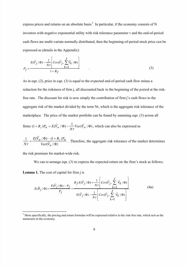
express prices and returns on an absolute basis.5
In particular, if the economy consists of N
investors with negative exponential utility with risk tolerance parameter τ and the end-of-period
cash flows are multi-variate normally distributed, then the beginning-of-period stock price can be
expressed as (details in the Appendix):
f R
J
k
k V jV Cov N
jV E
jP+
⎥⎥
⎦
⎤
⎢⎢
⎣
⎡
=Φ−Φ
=
∑
1
)
1
|~
,~
(1
)|~
(τ
. (3)
As in eqn. (2), price in eqn. (3) is equal to the expected end-of-period cash flow minus a
reduction for the riskiness of firm j, all discounted back to the beginning of the period at the risk-
free rate. The discount for risk is now simply the contribution of firm j’s cash flows to the
aggregate risk of the market divided by the term Nτ, which is the aggregate risk tolerance of the
marketplace. The price of the market portfolio can be found by summing eqn. (3) across all
firms: )|~
(1
)|~
()1( Φ−Φ=+ M M M f V Var N
V E P Rτ
, which can also be expressed as
)|~
()1()|
~
(1Φ
+−Φ=
M
M f M
V Var
P RV E
N τ . Therefore, the aggregate risk tolerance of the market determines
the risk premium for market-wide risk.
We can re-arrange eqn. (3) to express the expected return on the firm’s stock as follows.
L
emma 1. The cost of capital for firm j is
.
)|~
1
,~
(1
)|~
(
)|~
1
,~
(1
)|~
(
)|
~
()|~(
⎥⎥
⎦
⎤
⎢⎢
⎣
⎡Φ
=−Φ
⎥⎥
⎦
⎤
⎢⎢
⎣
⎡Φ
=
+Φ
=−Φ=Φ
∑
∑
k V J
k
jV Cov N
jV E
k V J
k
jV Cov N
jV E f R
jP jP jV E j R E
τ
τ (4a)
5 More specifically, the pricing and return formulas will be expressed relative to the risk-free rate, which acts as the
numeraire in the economy.
9

7/28/2019 Contabilitate si costul capitalului
http://slidepdf.com/reader/full/contabilitate-si-costul-capitalului 11/54
If we further assume that ,0)|V~
,V~
(Cov k
J
1k j ≠Φ∑
=this reduces to
)|
~
1,
~
(
1
)|~
()(,
1)(
1)()|
~(
Φ=
Φ=Φ
−Φ
+Φ=Φ
∑ k V
J
k jV Cov N
jV E H where
H
H f R j R E
τ
. (4b)
Lemma 1 shows that the cost of capital of the firm depends on four factors: the risk free
rate, the aggregate risk tolerance of the market, the expected cash flow of the firm, and the
covariance of the firm’s cash flow with the sum of all the firms’ cash flows in the market. The
latter three terms can be combined into the ratio of the firm j’s expected cash flows, to firm j’s
contribution to aggregate risk per-unit-of aggregate risk tolerance. Note that the definition of
cost of capital in Lemma 1 does not require that firm j’s expected cash flow, or the covariance of
that cash flow with the market, be of any particular sign.
In the next result we show how a change in each of the four factors affects cost of capital.
Proposition 1. Ceteris paribus the cost of capital for firm j, ),|~
( Φ j R E is:
(a) increasing (decreasing) in the risk free rate, R f , when the expected cash flow and the
price of the firm have the same (different) sign;
(b) decreasing (increasing) in the aggregate risk tolerance of the market, Nτ, when the
expected cash flow and covariance of that cash flow with the market have the same
(different) sign;
(c) decreasing (increasing) in the expected end-of-period cash flow, ) jV~
(E , when
)J
1k k V
~, jV
~(Cov ∑
=is positive (negative); and
(d) increasing (decreasing) in )J
1k k V
~, jV
~(Cov ∑
=when ) jV
~(E is positive (negative).
To make the intuition that underlies Proposition 1 as transparent as possible, consider the case in
which firm j’s expected end-of-period cash flow, the covariance between its end-of-period cash
10

7/28/2019 Contabilitate si costul capitalului
http://slidepdf.com/reader/full/contabilitate-si-costul-capitalului 12/54
flow and the market, and the firm’s beginning-of-period stock price are all positive. Here, the
reason why the expected return on firm j is increasing in the risk-free rate is clear, because this
provides the baseline return for all securities. When Nτ increases, the aggregate risk tolerance of
the market increases; hence, the discount applied to each firm’s riskiness decreases.6
This moves
the firm’s expected rate of return closer to the risk-free rate. When )J
1k k V
~, jV
~(Cov ∑
=increases,
the contribution of the riskiness of firm j’s cash flows to the overall riskiness of the market goes
up; hence, the expected return must increase to compensate investors for the increase in risk.
This is one of the key insights of the CAPM (Sharpe, 1964; Lintner, 1965).
Perhaps the most surprising result is that an increase in the expected value of cash flows
decreases the expected rate of return. The intuition, however, is fairly straightforward. Consider
a firm with two components of cash flow: a riskless component ( ) and a risky component
( ). Clearly the cost of capital for the firm will be somewhere in between the cost of capital
for the riskless component and the cost of capital for the risky component. But if the firm’s
expected cash flow increases without affecting the firm’s variances or covariances, this is exactly
analogous to adding a new riskless component of cash flows to the firm’s existing cash flows.
The firm’s cost of capital therefore decreases.
a j
V
b j
V
One potential concern may be that the effect of the expected cash flow on the expected
return is specific to the CARA, or negative exponential, utility function. We believe, however,
that this result is robust. To see this, note that the traditional CAPM formulation of pricing does
not assume negative exponential utilities. It only requires that cash flows are multivariate
normally distributed. To illustrate, we can start with our equation (2):
6 This is analogous to the effect discussed in Merton (1987).
11

7/28/2019 Contabilitate si costul capitalului
http://slidepdf.com/reader/full/contabilitate-si-costul-capitalului 13/54
1
( | ) ( , | )
(1 )
J
j j
k
j
f
E V Cov V V
P R
λ =
⎡ ⎤Φ − Φ⎢ ⎥
⎣ ⎦=+
∑% % %k
, where)|V
~(Var
P)R 1()|V~
(E
M
Mf M
Φ
+−Φ=λ is a market-wide
parameter. Using the same steps as the derivation in Proposition 1, we can write the expected
return on firm j's stock as:
,1H
1HR
P
P)V(E)R (E f
j
j j j +
−=
−= , where now H = .
1
),(
)(
∑=
J
jk V jV Cov
jV E
λ
Assuming the impact of a single firm is small relative to the market as a whole, such that the
market-wide term, λ , is unaffected, the comparative statics in Proposition 1 go through. In
particular, the expected return is decreasing in E(Vj), ceteris paribus. Obviously, the assumption
that the market-wide term is unaffected is “less clean” than our prior derivation, which is why we
add structure by assuming the negative exponential utility. It seems clear, however, that the
result will hold in far more general terms.
The results in Proposition 1 vary one parameter at a time, holding the others constant.
But what if the expected cash flows and the covariance change simultaneously? For the special
case where expected cash flows and the covariance both change in exactly the same proportion,
it is easy to see that the numerator and denominator each change by that proportion in eqn. (4),
and thus cancel out. In this special case, there is no effect on the cost of capital. There is an
effect, however, for any simultaneous change that is not exactly proportionate on the two terms.
While it is common in some corporate finance and valuation models to assume that the
level of cash flow and the covariances move in exact proportion to each other (i.e., all cash flows
are from the same risk class), we are unaware of any theoretical results or empirical evidence to
suggest this should be the case. On the contrary, the existence of fixed costs in the production
12

7/28/2019 Contabilitate si costul capitalului
http://slidepdf.com/reader/full/contabilitate-si-costul-capitalului 14/54
function, economies of scale, etc., generally make the expected values and covariances of firm’s
cash flows change in ways that are not exactly proportional to each other. Moreover, there is
ample empirical evidence that betas vary over time, which implies the ratio of expected cash
flow to overall covariance varies, suggesting that new information has an impact as it becomes
available.7
There is nothing in Proposition 1 that is specific to accounting information. Any shock –
new regulations, taxes, inventions, etc. – that affects the H term has a corresponding effect on the
firm’s expected return. In the following two sections we focus on how accounting information
impacts the H(Φ) ratio in the cost of capital equation. In section 3, we show how, holding the
real decisions of the firm fixed, accounting information affects the assessments made by market
participants of the distribution of future cash flows, and how this assessment impacts the firm’s
cost of capital. In section 4, we show that accounting information affects real actions within the
firm, and that this naturally leads to changes in the risk-return characteristics of the firm, thereby
affecting the firm’s cost of capital.
7 Our model is one-period model, which implies that the end-of-period cash flows are consumed by shareholders.
More generally, in a multiperiod model, these cash flows could be re-invested in the firm. Our analysis does not
make any assumptions about the nature of the re-investment policy. If the end result of an increase in expected cashflows combined with a re-investment policy results in a change in the parameter H, i.e., ratio of the expected cash
flows to the covariance with all other firms, the cost of capital will change. The re-investment policy will depend onthe nature of the investment opportunity set and the manager’s incentives. One scenario where the overall effect
might be zero is the one where the new cash flows are re-invested in exactly the same risk-return profile as the firm'sother projects. For any other investment policy, the expected return changes. For example, if managers have an
incentive to “hoard” excess cash, as suggested by the literature on the free-cash flow problem, then the effects do not
exactly offset each other. Our model applies to any re-investment policy, and the overall effect on the firm's cost of capital can be thought of as the sum of two (potentially offsetting) effects: (a) the effect of the cash flow shock per
se, and (b) the change (if any) in the distribution of cash flows due to the investment policy. This latter effect is
analogous to our “real effects” analysis in Section 4. Our analysis also provides sufficient conditions where these
two effects do not offset (see Proposition 4).
13

7/28/2019 Contabilitate si costul capitalului
http://slidepdf.com/reader/full/contabilitate-si-costul-capitalului 15/54
3. Direct Effects of Information on the Cost of Capital
In this section, we add a general information structure to the model, which allows us to
analyze the direct effects of information quality on the cost of capital. To do so, we hold the
firm’s real (operating, investing, and financing) decisions constant (we relax this in Section 4).
Even though accounting and disclosure policies do not affect the real cash flows of the firm here,
they change the assessments that market participants have regarding the distribution of these
future cash flows. As a result, they affect equilibrium stock prices and expected returns. In
particular, eqns. (3) and (4) show that stock price and the expected return are, respectively,
decreasing and increasing functions of the covariance of a firm’s end-of-period cash flow with
the sum of all firms’ end-of period cash flows. In the next two sub-sections, we discuss the two
components of this covariance: the firm’s own variance and the covariances with other firms,
).~
,~
()~
,~
()~
,~
(1
∑≠ jk
k j j j
J
k k j V V CovV V CovV V Cov
3.1 Direct Effects – Through the Variance of the Firm’s Cash Flow
The idea that better quality accounting information reduces the assessed variance of the
firm’s cash flow is well known. As an application, consider the impact on the cost of capital of
firm j if more information becomes available (either through more transparent accounting rules,
additional firm disclosure, or greater information search by investors). Suppose the firm’s
investment decisions have been made; let V0j and jω represent the ex-ante expected value and
ex-ante precision of the end-of-period cash flow, respectively. Suppose investors receive Q
independently distributed observations, z j1,...,z jQ, about the ultimate realization of firm j’s cash
14

7/28/2019 Contabilitate si costul capitalului
http://slidepdf.com/reader/full/contabilitate-si-costul-capitalului 16/54
flow, where each observation has precision jγ . Then investors’ posterior distribution for end-
of-period cash flow has a normal distribution with mean
=),...,|~
( 1 jQ j j z zV E ∑+
++ =
Q
q jq
j j
j j
j j
j z
QV
Q 10
γ ω
γ
γ ω
ω , and precision jQ j γ+ω .
The analysis above formalizes the notion that accounting information and disclosure reduce the
assessed variance of the firm’s end-of-period cash flows. In particular, the assessed variance
decreases (equivalently, the assessed precision increases) with 1) an increase in the prior
precision, ω j; 2) the number of new observations, Q; or 3) the precision of these observations, γ j.
Since the assessed variance of the firm’s cash flow is one of the components of the
covariance of the firm’s cash flow with those of all firms, then using part (d) of Proposition 1,
ceteris paribus, reducing the assessed variance of the firm’s cash flows increases the firm’s stock
price and reduces the firm’s expected return. Moreover, because the variance term is an
additively separate term in the overall covariance, the magnitude of this impact on price does not
depend on how highly the firm’s cash flows co-vary with those of other firms. For example, a
decrease of, say, 10 percent in the assessed variance of firm cash flows has the same dollar effect
on stock price regardless of the degree of covariance with other cash flows. Therefore, for a
given finite value of N (the number of investors) and J (the number of firms in the economy),
there is a non-zero effect on price and on the cost of capital of reducing the assessment of firm-
variance.
The firm-specific variance reduction effect is an important factor in the cost of capital
analysis of Easley and O’Hara (2004). While their paper models a multi-security economy, their
assumption that all cash flows are independently distributed implies that the pricing of each firm
15
7/28/2019 Contabilitate si costul capitalului
http://slidepdf.com/reader/full/contabilitate-si-costul-capitalului 17/54
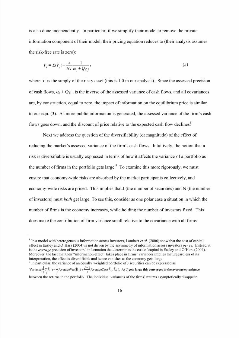
is also done independently. In particular, if we simplify their model to remove the private
information component of their model, their pricing equation reduces to (their analysis assumes
the risk-free rate is zero):
j j j j
Q N
xV E P
γ ω τ +−
1)
~( , (5)
where x is the supply of the risky asset (this is 1.0 in our analysis). Since the assessed precision
of cash flows, ω j + Qγ j , is the inverse of the assessed variance of cash flows, and all covariances
are, by construction, equal to zero, the impact of information on the equilibrium price is similar
to our eqn. (3). As more public information is generated, the assessed variance of the firm’s cash
flows goes down, and the discount of price relative to the expected cash flow declines.8
Next we address the question of the diversifiability (or magnitude) of the effect of
reducing the market’s assessed variance of the firm’s cash flows. Intuitively, the notion that a
risk is diversifiable is usually expressed in terms of how it affects the variance of a portfolio as
the number of firms in the portfolio gets large.9
To examine this more rigorously, we must
ensure that economy-wide risks are absorbed by the market participants collectively, and
economy-wide risks are priced. This implies that J (the number of securities) and N (the number
of investors) must both get large. To see this, consider as one polar case a situation in which the
number of firms in the economy increases, while holding the number of investors fixed. This
does make the contribution of firm variance small relative to the covariance with all firms
8 In a model with heterogeneous information across investors, Lambert et al. (2006) show that the cost of capital
effect in Easley and O’Hara (2004) is not driven by the asymmetry of information across investors per se. Instead, itis the average precision of investors’ information that determines the cost of capital in Easley and O’Hara (2004).
Moreover, the fact that their “information effect” takes place in firms’ variances implies that, regardless of its
interpretation, the effect is diversifiable and hence vanishes as the economy gets large.9 In particular, the variance of an equally weighted portfolio of J securities can be expressed as
covarianceaveragethetoconvergesthislargegetsJAs.)R ~
,R ~
(AverageCovJ
1J)R
~(AverageVar
J
1)R
~
J
1(Variance
jk j j j∑
−+=
between the returns in the portfolio. The individual variances of the firms’ returns asymptotically disappear.
16

7/28/2019 Contabilitate si costul capitalului
http://slidepdf.com/reader/full/contabilitate-si-costul-capitalului 18/54
(assuming firms’ covariances tend to be positive). It also increases, however, the aggregate risk
in the economy: that is, increases without bound. This drives prices lower and
results in an infinite increase in the expected return required to hold the stock (see eqns. [3] and
[4]). On the other hand, consider as the other polar case a situation where N, the number of
investors in the economy, alone grows large. This will result in spreading all risks (not just
firms’ variances) over more investors, which reduces all risk premiums and decreases all
expected returns. In the limit,
∑=
J
k k j V V Cov
1
)~
,~
(
∑=
J
k k j V V Cov
N 1
)~
,~
(1
approaches zero for each firm and even for the
market; therefore, no risks are priced. To avoid these uninteresting, polar cases, J and N must
both increase for the notion of “diversifiability” to be meaningful.
When J and N both increase, the effect of firm-variance on the cost of capital,
),~
,~
(1
j j V V Cov N τ
asymptotically approaches zero, because this term only appears once in the
overall covariance for a firm.10
The covariance with other firms, however, ,)~
,~
(1
∑≠ jk k jV V Cov
N τ
survives because the number of covariance terms (J-1) also increases as the economy gets large.
In the next section, we analyze how information affects the covariance terms.
3.2 Direct Effect – Through the Covariance with other Firms’ Cash Flows
In this section, we show that information about a firm’s future cash flows also affects the
assessed covariance with other firms. Our work in this section builds on the estimation risk
10 In our simplified version of the Easley and O’Hara result (our eqn. [5]), as N gets large, the last term on the right-hand side of the equation approaches zero. Therefore, the firm is priced as if it is riskless (recall that Easley and
O’Hara assume there are no covariances with other firms). Similarly, in their “full blown” model (see their
proposition (2), as N gets large the per-capita supply of the firm’s stock goes to zero, and again the pricing equation
collapses to a risk-neutral one.
17

7/28/2019 Contabilitate si costul capitalului
http://slidepdf.com/reader/full/contabilitate-si-costul-capitalului 19/54
literature in finance (See Brown,1979; Barry and Brown;1984 and 1985; Coles and
Loewenstein,1988; and Coles et al., 1995). Specifically, our work differs from this literature in
three important ways. First, the estimation risk literature generally focuses on the impact of the
information environment on the (return) beta of the firm, whereas our focus is on the cost of
capital. Because the information structures analyzed in this literature generally affect all firms in
the economy, the impact on beta is confounded by the simultaneous impact on the covariances
between firms and the variance of the market portfolio. This is one reason why they obtain
results that are mixed or difficult to sign. By focusing on the cost of capital, we can analyze the
impact of both effects.
Second, the estimation literature focuses on very specific changes in the information
environment. Some papers examine the impact of increasing equally the amount of information
for all firms. Other papers compare two information environments: an environment where the
amount of information is equal across all firms to an environment where investors have more
information for one subgroup of firms than they do for a second group. Our framework allows
us to analyze more general changes in information structures: both mandatory and voluntary. In
particular, unlike the prior literature, we are able to address the question of how more
information about one firm affects its cost of capital within an unequal information environment .
Finally, our model represents information differently than in the estimation risk literature.
The estimation risk literature assumes the information about firms arises from historical time-
series observations of firms’ returns. While this literature claims that the intuition behind their
results applies to information more generally, the assumed time-series nature of their
characterization of information drives a substantial element of the covariance structure in their
18

7/28/2019 Contabilitate si costul capitalului
http://slidepdf.com/reader/full/contabilitate-si-costul-capitalului 20/54
models. In particular, new information is correlated conditionally with contemporaneous
observations and conditionally independent of all other information.11
We model a more general information structure that allows us to examine alternative
covariance structures. Specifically, we model information as representing noisy measures of the
variables of interest, which are end-of-period cash flows. That is, an observation, ,Z~
j about
firm j’s cash flow, ,V~
j is modeled as ,~~~ j j j V Z ε += where jε ~ is the “noise” or “measurement
error” in the information. Depending on the correlation structure assumed about the cash flows
and error terms, jZ~
could also be informative about the cash flow of other firms, as well as
informative in updating the assessed variances and covariances of end-of-period cash flows.
This formulation of information is consistent with the way information is modeled in virtually all
conventional statistical inference problems (see DeGroot, 1970). It is also consistent with
virtually all papers in the noisy rational expectations literature in accounting and finance (see
Verrecchia, 2001, for a review).
Our characterization of disclosures as noisy information about firms’ future cash flows
(or other performance measures) also comports well with actual disclosure practices. Firms’
earnings provide information about the sum of the market, industry, and idiosyncratic
components of their future cash flows.12
Similarly, other disclosures such as revenues or a cash
flow statement are typically for the firm as whole. Analysts’ forecasts of future earnings are also
about the earnings of the entire firm, not just of the idiosyncratic component of future earnings.
11 See Kalymon (1971) for the original derivation of the covariance matrix used in much of this literature.
12 In contrast, Hughes et al. (2005) artificially decompose information into “market” and “idiosyncratic factors.”Moreover, in our model cash flows have a completely general variance-covariance structure, whereas the analysis in
Hughes et al. assumes a very specific “factor” structure. Similarly, the betas and covariances that turn out to be
relevant in our pricing equations are relative to the market portfolio (the sum of all firm’s cash flows), whereas in
Hughes et al. the betas and covariances are relative to the exogenously specified “common factors.”
19

7/28/2019 Contabilitate si costul capitalului
http://slidepdf.com/reader/full/contabilitate-si-costul-capitalului 21/54
There is also substantial empirical support for the notion that the earnings of a firm can
be useful in predicting future cash flows of the industry or the market as a whole. As far back as
Brown and Ball (1967) studies have documented substantial market and industry components to
firms’ earnings. Bhoraj et al. (2003) extend this finding to other firm-level variables and
financial ratios. The “information transfer” literature also documents relationships between
earnings announcements by one firm and the earnings or stock price returns of other firms (e.g.,
Foster, 1981; Hand and Wild, 1990; Freeman and Tse, 1992). Piotroski and Roulstone (2004)
document how the activities of market participants (analysts, institutional traders, and insiders)
impact the incorporation of firm-specific, industry and market components of future earnings
into prices. As we show, it is not necessary that there be a “large” effect of firm j’s disclosures
on individual other firms.
Consider first the case of two firms and suppose that the future cash flows of the two
firms have an ex-ante covariance of )~
,~
( k j V V Cov , which is non-zero. Suppose further that we
observe ,~ j Z which is noisy information about firm j’s future cash flow, .
~ jV As in the previous
section, the posterior variance of jV ~
becomes smaller as the precision of j Z ~
increases.
Moreover, we can show that the information j Z ~
leads to an updated assessed covariance
between the two cash flows jV ~
and .~k V In particular, it is straightforward to show that the
updating takes the following form.
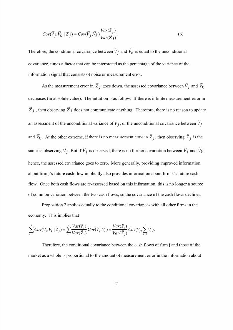
Proposition 2. The covariance between the cash flows of firms j and k conditional on
information about firm j’s cash flow moves away from the unconditional )~
,~
( k V jV Cov and
closer to zero as the precision of firm j’s information increases. Specifically,
20
7/28/2019 Contabilitate si costul capitalului
http://slidepdf.com/reader/full/contabilitate-si-costul-capitalului 22/54
.)
~(
)~()
~,
~()|
~,
~(
j Z Var
jVar k V jV Cov j Z k V jV Cov
ε = (6)
Therefore, the conditional covariance between jV ~
and k V ~
is equal to the unconditional
covariance, times a factor that can be interpreted as the percentage of the variance of the
information signal that consists of noise or measurement error.
As the measurement error in j Z ~
goes down, the assessed covariance between jV ~
and k V ~
decreases (in absolute value). The intuition is as follow. If there is infinite measurement error in
j Z ~
, then observing j Z ~
does not communicate anything. Therefore, there is no reason to update
an assessment of the unconditional variance of jV ~
, or the unconditional covariance between jV ~
and k V ~
. At the other extreme, if there is no measurement error in j Z ~
, then observing j Z ~
is the
same as observing jV ~
. But if jV ~
is observed, there is no further covariation between jV ~
and k V ~
;
hence, the assessed covariance goes to zero. More generally, providing improved information
about firm j’s future cash flow implicitly also provides information about firm k’s future cash
flow. Once both cash flows are re-assessed based on this information, this is no longer a source
of common variation between the two cash flows, so the covariance of the cash flows declines.
Proposition 2 applies equally to the conditional covariances with all other firms in the
economy. This implies that
1 1
( ) ( )
( , | ) ( , ) ( , ).( ) ( )
J J j j
j k j j k j k k k j j
Var Var
Cov V V Z Cov V V Cov V V Var Z Var Z 1
J
k
ε ε
= == =∑ ∑
% %% % % % % %
% % =∑
Therefore, the conditional covariance between the cash flows of firm j and those of the
market as a whole is proportional to the amount of measurement error in the information about
21

7/28/2019 Contabilitate si costul capitalului
http://slidepdf.com/reader/full/contabilitate-si-costul-capitalului 23/54
firm j’s cash flow. Moreover, this effect does not diversify away in large economies: the effect
is present for each and every covariance term with firm j.
Note that Proposition 2 does not require that the unconditional covariance be positive.
As the measurement error in j Z ~
goes down, the assessed covariance between jV ~
and
moves closer to zero, irrespective of its sign. If the unconditional covariance is negative, then
the conditional covariance increases toward zero. In this case, improved information will
increase the firm’s cost of capital. The reason for the increase is that a firm with a negative
(unconditional) covariance between its cash flow and the market cash flow sells at premium
reflecting that it offers a counter-cyclical cash flow. Anything that makes the negative
covariance less negative, such as more precise information, reduces the premium, and thus
increases that firm's cost of capital.
1
J
k
k
V =
∑ %
We can also express our findings for the (special) case where the distribution of cash
flows is represented by a “single-factor index model,” which is commonly used in finance.
Suppose that the cash flow for firm j is ,~ j j j j ubaV +θ where θ is a “market factor” and u j is
a firm specific factor. For convenience, let all the u j’s be distributed independently. Let the
information about firm j be a noisy measure of its cash flow, j jV j Z ε ~~~
+= , where the error
terms are distributed independently of the true cash flows, as well as each other. Then the
unconditional covariance between the cash flows of firms j and k is b j bk Variance(θ), and the
conditional covariance given Z j is
,)(
)()()|
~,
~(
j Z Variance
jVarianceVariancek b jb j Z k V jV Cov
ε θ = which implies
22

7/28/2019 Contabilitate si costul capitalului
http://slidepdf.com/reader/full/contabilitate-si-costul-capitalului 24/54
.)(
)()()|
~,
~( ∑∑
≠=
≠ jk k b
j Z Variance
jVarianceVariance jb j Z k V
jk jV Cov
ε θ
As before, the posterior covariance between firm j and “the market” gets closer to zero as the
quality of the information about firm j’s future cash flow improves.
As noted above, our information structure implies that an infinitely precise information
system perfectly reveals a firm’s future cash flow. Of course, in reality we would not expect
even the most precise disclosure and accounting system to remove all uncertainty about a firm’s
future cash flow. It is straightforward to incorporate a limit on how precise the information can
be regarding future cash flows and our results continue to hold. One interpretation of this limit is
that it represents the distinction between “fundamental” or “technological” risk, as opposed to
“estimation risk.” While this distinction has some intuitive appeal, even “fundamental risk” is
conditional upon the information system available. Our analysis does not rely on the (somewhat
arbitrary) distinction between estimation and fundamental risk; nonetheless, it would continue to
hold if such a distinction were modeled formally.
Similarly, another possible extension is to change the underlying construct that governs
information. Consistent with the way information is modeled in most of the rational
expectations literature, in our paper we interpret information as being related to the realized
future cash flow. We could also conduct the analysis by interpreting information instead as
signals about the expected future cash flow (or about parameters of the distribution of future cash
flows). In fact, most of the estimation risk literature interprets information this way. Of course,
when learning about the expected future cash flow, as opposed to the realized future cash flow, a
perfect signal no longer resolves all uncertainty. In that case, the remaining uncertainty could be
interpreted as “fundamental risk” as discussed above. The insights from our analysis apply as
23
7/28/2019 Contabilitate si costul capitalului
http://slidepdf.com/reader/full/contabilitate-si-costul-capitalului 25/54
long as some residual uncertainty remains. We could also repeat the analysis under alternative
assumptions regarding which parameters of the distribution of future cash flows are uncertain:
1) the expected future cash flows are unknown but the covariance matrix is known; or 2) the
expected future cash flows and the covariance matrix are both unknown.
Our finding that information affects the assessed covariance between firms’ cash flows
are in contrast to those in a concurrent paper by Hughes et al. (2005), which employs more
restrictive and less natural information structures. For example, Hughes et al. show that if the
information concerns exclusively the idiosyncratic component of a firm's cash flows, not the
cash flows per se, and the information matrix is exclusively diagonal then there is no covariance
effect. That is, under these conditions, the information is, by definition, unrelated to the
component of cash flows that varies across firms, so they cannot be useful in updating the
assessed covariance.
Hughes et al. also considers an information structure that relates only to the “common
factor” portion of cash flows. In this case, information does affect the covariance between a
firm’s cash flows and the common factors. Similarly, the covariance between the cash flows of
any two firms that are both affected by this common factor will also change. While this result is
similar in some ways to ours, the nature of the cross-sectional impact on the covariance, and
therefore the cost of capital, differs in their paper because of the different information structure
assumed.
When the information is about the firm’s cash flow as a whole, we find that virtually any
more general representation of firms’ cash flows and information will change the covariance of
jV ~
and k V ~
. For example, a natural extension of Proposition 2 is to consider the impact on the
covariance of both firms providing information. When the measurement errors in the
24

7/28/2019 Contabilitate si costul capitalului
http://slidepdf.com/reader/full/contabilitate-si-costul-capitalului 26/54
information across firms are conditionally uncorrelated, the analysis in Proposition 2 extends
easily.13
Another interesting extension is to analyze the case of correlated measurement errors in
the accounting information across firms. It seems intuitive that firms using the same (imperfect)
financial reporting principles have correlated measurement errors, as well as correlated cash
flows. In general, the conditional covariance of firm j’s cash flows will still be affected by the
amount of measurement error in both firm j’s and firm k’s accounting information, but signing
the effect is more difficult. Unfortunately there is little precedent in the statistical decision
theory literature or the estimation literature in finance for how to model information when key
elements are correlated.
In particular, in order to carry out any analysis, it important to be able to specify how the
covariance between the measurement errors in firms’ disclosures changes as the quality of one
firm’s accounting information improves. One possibility is to assume that the correlation, ρ,
between measurement error terms remains constant, so that the covariance between the two
measurement error terms is equal to this correlation coefficient times the standard deviations of
the two firms’ error terms. In this case, lowering the measurement error in firm j’s disclosure,
the variance of ε j in our notation, lowers proportionately the covariance between the error terms
in the information firms j and k’s provide. While the equation is difficult to sign in general, we
provide in a Corollary to Proposition 2 (see the Appendix) sufficient conditions for a decrease in
the measurement error of firm j’s accounting information to move the conditional covariance
between firm j and k’s cash flow toward zero.
Thus, we claim that in general information about firm cash flows (or other measures of
13 See the discussion of the Corollary that follows the proof to Proposition 2 in the appendix.
25

7/28/2019 Contabilitate si costul capitalului
http://slidepdf.com/reader/full/contabilitate-si-costul-capitalului 27/54
firm performance) has a covariance effect, and hence leads to cross-sectional differences in
firms’ cost of capital. It is important to point out that, even in the case where all firms provide
information, it is not necessarily the case that the uncertainty about the market cash flow is
eliminated. If each firm discloses its realized cash flow with noise, uncertainty about the market
cash flow will grow as the number of firms in the economy grows.14
3.3 The Effects of Mandatory Disclosures
In the previous sections, we analyze the impact of changing the quality of accounting
information for a single firm on its price and cost of capital. We now briefly discuss the effects
of mandatory disclosure of accounting information. The main difference is that disclosure
regulation affects all firms. Therefore, in addition to the impact of firm j’s disclosure on, say, the
covariance between the cash flows of firms j and k, firm k’s disclosures have an additional
impact on this covariance. In principle, disclosure by every other firm could have a (small)
impact on its covariance with firm j. That is, each firm’s disclosure generates an externality on
other firms’ cost of capital. This positive externality provides potentially a reason why there
could be benefits to disclosure regulation, rather than relying on voluntary disclosures, because
firms will not take this externality into account when deciding the optimal level of voluntary
disclosure. While this effect is small individually, it could become large collectively.15
Based on our framework and prior results, increasing the quality of mandated disclosures
should in general reduce the cost of capital for all firms in the economy (assuming that the
expected cash flow of each firm in the economy and the covariance of that firm’s cash flow with
14 In contrast, if each firm discloses the aggregate market cash flow with idiosyncratic noise, the disclosures of manyfirms would in the limit reveal the market cash flow, and there would be no aggregate uncertainty. This information
structure, however, is not very descriptive of what firms do.15 See Fishman and Hagerty (1989), Dye (1990), and Admati and Pfleiderer (2000) for other externality-based
explanations of mandatory disclosure.
26
7/28/2019 Contabilitate si costul capitalului
http://slidepdf.com/reader/full/contabilitate-si-costul-capitalului 28/54
the market have the same sign). The precise effect, however, may depend on how the
covariances of the measurement errors are affected and hence is subject to the discussion at the
end of the previous section (see also the Corollary to Proposition 2).
In addition, the magnitude of the impact of mandatory disclosure on a particular firm’s
cost of capital is less clear-cut. Even if mandatory disclosures affect all elements of the
covariance matrix of future cash flows by a scale factor, the effect on the cost of capital is not
proportionate for all firms. In particular, it follows from the pricing formula in eqn. (2) that the
cost of capital depends on the ratio of the firm’s expected cash flow to its covariance with all
cash flows. Even if all firms’ covariances were affected proportionately, their expected cash
flows would be unlikely to have the same scale factor. Therefore, the prices of all firms will not
change proportionately. Thus, using eqn. (4), the firms’ expected returns (and cost of capital)
will not change by the same proportion for all firms either.16
Moreover, it seems unlikely that mandated disclosures would alter the entire covariance
matrix of all firms’ future cash flows by the same scale factor. The amount of new information
provided by a particular mandated disclosure depends on what other information the firm already
discloses. For some firms, this disclosure requirement duplicates other disclosures, in which
case it provides no additional information; for others it may provide a small amount of
incremental information, and for others still it may be completely new. These information
effects imply an unequal impact of disclosure regulation on the individual elements of the
16 Some early models in the estimation risk literature in finance (e.g., Kalymon, 1971; Brown, 1979) assumed thatinformation had a proportionate impact on the covariance matrix of returns, and some found that information would
not affect the betas of firms. This result occurred because (by assumption) all the covariances and variances of
firms’ returns changed proportionately. Therefore, there was no affect on the beta coefficient of returns, which is theratio of the covariance of the firm’s return to the market divided by the variance of the market return, because the
numerator and denominator changed by the same scale factor. It is more natural to assume, however, that the impact
of information is on the assessed distribution of cash flows, not returns. See Coles and Lowenstein (1988) for
similar discussion.
27

7/28/2019 Contabilitate si costul capitalului
http://slidepdf.com/reader/full/contabilitate-si-costul-capitalului 29/54
covariance matrix of future cash flows. Thus, firms are likely to be affected by mandatory
disclosures differentially.
It is important to distinguish between the impact of mandated disclosure on the cost of
capital and the impact on the beta coefficient. Our formulation allows us to express the cost of
capital in a reduced form that depends on assessed covariance between the cash flow of the firm
and the cash flows of all firms in the market. Even if mandated disclosure reduced the cost of
capital for firms, this does not imply that all beta coefficients will be similarly reduced. Instead,
the lowered covariance between end-of-period cash flows implies a reduction in the product of
the impact on the market risk premium and the beta coefficient; it does not imply a reduction in
the beta coefficient separately. In fact, the average beta in the economy must still be 1.0,
regardless of the quality of the information environment. Therefore, mandated disclosure cannot
reduce all firms’ betas. This insight suggests that researchers interested in examining the effect
of mandated disclosures on costs of capital must look beyond the beta coefficient and examine
aggregate measures such as the average cost of capital in the economy or the market risk
premium.
4. Indirect Effects of Information on Cost of Capital
In this section, we show how the quality of the accounting and disclosure system has an
indirect impact the firm’s cost of capital through its effect on real decisions that impact the
expected cash flows and covariances of cash flows. Clearly, decision-makers in an economy
make decisions on the basis of the information they have available to them. If this information
changes, so will their decisions. To the extent these new decisions alter the distribution of the
firm’s end-of-period-cash flow, this impacts the firm’s cost of capital. In particular, as we
showed in Proposition 1, if the ratio of the firm’s expected cash flow to the covariance between
28

7/28/2019 Contabilitate si costul capitalului
http://slidepdf.com/reader/full/contabilitate-si-costul-capitalului 30/54
the firm’s cash flow and the sum of all other firms’ cash flows changes (our parameter H in our
Lemma 1), the expected rate of return on the firm’s stock will change, and by definition, so will
its cost of capital.
The potential scope of the decisions that a firm’s accounting and disclosure systems may
affect can be broad. In addition to the decisions of investors and creditors, a firm’s accounting
and disclosure systems may affect managerial actions, as well as the potential actions of
competitors, regulatory authorities, etc. The impact on the firm’s cost of capital can be either
positive or negative. To be able to predict the “indirect effect” of accounting information on the
firm’s cost of capital therefore requires the researcher to carefully specify: 1) the link between
information and these decisions; and 2) the impact of these decisions on the distribution of future
cash flows. We provide two simple examples to illustrate these issues. In one, accounting
information affects the amount of cash that is appropriated from investors. In the second,
accounting information changes a manager’s investment decisions.
4.1 Information, Governance, and Appropriation
Many papers (e.g., in agency theory) have suggested that better financial reporting and/or
corporate governance increases firm value by reducing the amount that managers appropriate for
themselves (e.g., LaPorta et al., 1997; Lambert, 2001). These papers, however, do not discuss the
impact that these systems have on the firm’s cost of capital. In fact, some of them claim that
these systems have a “one-time” effect on price, but do not affect the cost of capital as defined
by the discount rate implicit in the firm’s stock valuation. An exception is Lombardo and
Pagano (2000), as they also analyze the impact of governance and appropriation on firm’s cost of
capital. We compare our model and results to Lombardo and Pagano (2000) below.
29

7/28/2019 Contabilitate si costul capitalului
http://slidepdf.com/reader/full/contabilitate-si-costul-capitalului 31/54
Represent the “gross” end-of-period cash flow of firm j before any appropriation by .~* jV
As before, we assume this cash flow has a normal distribution. Managers appropriate for
themselves an amount A that decreases with the quality of the information and/or governance
systems. By accounting systems here, we do not mean simply the disclosures the firm makes to
outsiders, but also internal control systems, corporate governance policies, etc.17 Clearly, a more
sophisticated analysis could be conducted that endogenously derives the functional form of A
and/or determines the types of information that lead to the largest reductions in A, but these
features are not necessary to make our point.
In particular, the amount of the firm’s end-of-period cash flows that is appropriated from
shareholders is , where Q is the quality of the accounting and disclosure
system, A
*
10 )()()( jV Q AQ AQ A +=
0 is non-negative, A1 is between 0 and 1, and V* is the value of the firm gross of any
appropriation.18
A higher quality accounting system is assumed to reduce the amount of
misappropriation: and . This means that the net amount received by the firm’s
shareholders is
0A0 ≤′ 0A1 ≤′
).(0*~
))(11()(*~~Q A jV Q AQ A jV jV −−=−=
This representation allows us to calculate the expected value of the firm’s cash flow and its
covariance with other firms’ cash flows as a function of the quality of the information and/or
17 More generally, the amount a manager could appropriate would also depend on dimensions of the legal system,
such as the ability to bring lawsuits against the firm and/or managers. Note that for convenience, we have
suppressed the subscript j on the parameters A0 and A1.
18 Lombardo and Pagano (2000) analyze a model that also has a parameter analogous to our A1, which reduces thecash flow available to shareholders by a fractional amount. They do not have a parameter, however, that corresponds
exactly to our A0, which reduces the end-of-period cash flow by a constant. Instead, they have a cost that
shareholders pay out of their own pocket for auditing and legal fees. This fee is proportional to the share price,which obviously depends on the expected end-of-period cash flow. Another difference is that in their model
appropriation parameters are economy-wide (or for segments of the market), whereas ours can be firm-specific.
Finally, we explicitly analyze the impact the appropriation parameters have on the riskiness of the end-of-period
cash flow (variances and covariances), whereas these are not issues addressed in Lombardo and Pagano (2000).
30

7/28/2019 Contabilitate si costul capitalului
http://slidepdf.com/reader/full/contabilitate-si-costul-capitalului 32/54
governance quality parameter, Q. We can then apply Lemma 1 to determine the effect on the
firm’s cost of capital.
Proposition 3. Higher quality information that reduces managerial misappropriation of the
firm’s cash flow weakly moves the firm’s cost of capital toward the risk-free rate. If A0 = 0 and
(so that information only affects the A0A0 =′ 1 term), then information has no effect on the cost
of capital. Otherwise, improved information moves the cost of capital closer to the risk-free rate.
One special case arises when the quality of the information and/or governance system
affects only the “fixed amount” (A0) the manager appropriates. In this case, increasing the
quality of the accounting system increases the expected cash flow available to shareholders by
reducing A0. It does not affect, however, the covariance of the firm’s net cash flows with those
of other firms. Therefore, not surprisingly, a higher quality accounting system increases the price
of the firm. What is more surprising is that the information system also leads to a change in the
firm’s cost of capital. Our model shows that the reason is straightforward: the ratio of the
expected cash flows to the covariance shifts.
At the other extreme, suppose the quality of information affects only the “proportion” of
the firm’s cash flow the manager appropriates: the parameter A1. In this case, improving the
quality of the firm’s information and/or governance system increases the proportion of the firm’s
cash flow available to shareholders. This not only increases the firm’s expected cash flow, but it
also increases the covariance of the firm’s cash flows with other firms by the same proportion.
Therefore, the ratio of expected cash flow to covariance of cash flows does not change, and the
firm’s cost of capital is unaffected.19
Lombardo and Pagano (2000) establish a similar result:
19 Technically, the total covariance does not change in exact proportion to the expected value because the firm’s
covariance with itself will change with the square of the proportionality factor. As in the previous section, however,
the impact of the firm’s own variance on the cost of capital goes to zero as the number of investors gets large. In
31

7/28/2019 Contabilitate si costul capitalului
http://slidepdf.com/reader/full/contabilitate-si-costul-capitalului 33/54
price increases, but there is no impact on the firm’s expected rate of return given this “one time”
effect on price.
In fact, Proposition 3 indicates that the assumption that the manager’s appropriation is
exactly a fixed proportion of the end-of-period cash flow is the only situation in which there is
no impact on the cost of capital. As long as there is a component of appropriation that does not
vary with the realization of the end-of-period-cash flow (for example, if it depends on the
expected future cash flow instead of its realization), or the quality of information affects the
“fixed” component of appropriation, there will be a non-zero impact on the cost of capital.
We can also interpret the parameters A0 and A1 as cash flow appropriated by other firms,
as opposed to by the manager. This allows us to tie our results to the large literature in
accounting on the proprietary costs of disclosure (see Verrecchia, 2001). In this literature,
increased disclosure allows other firms to make better strategic decisions to compete away some
of the profits of the disclosing firm We can adapt our model to this situation by assuming that
increased disclosure quality will increase A0 or A1. The comparative statics are straightforward,
and in this case increased disclosure quality weakly increases the firm’s cost of capital. A
common assumption in the literature for the functional form of the proprietary costs is that they
reduce profits by a constant (e.g., Verrecchia, 1983). In this case, improved accounting
information and disclosure increases A0, and strictly increases the firm’s cost of capital.
Finally, suppose improved accounting and disclosure influences the governance of all
firms, as in a mandatory change such as the Sarbanes-Oxley Act of 2002. Again, the impact of
the indirect effects on the cost of capital is ambiguous. As above, if improved disclosure shifts
only the “fixed” component of managerial misappropriation, firms’ cost of capital decreases.
this case, the impact of an improvement on the firm’s expected cash flows will be approximately proportionate to
the change in the overall covariance, in which case the impact on the cost of capital will be approximately zero.
32

7/28/2019 Contabilitate si costul capitalului
http://slidepdf.com/reader/full/contabilitate-si-costul-capitalului 34/54
The results are different, however, for the case where improved disclosure impacts only the
proportion (A1) of the cash flow appropriated by the manager.20
As above, the firm’s expected
cash flow rises by a factor of (1-A1). However, because the cash flows of all firms shift
proportionately, the covariances of cash flows increase by a factor of (1-A1)2. In this case,
mandatory disclosure increases the firm’s cost of capital.
While this result might seem unintuitive, the reason is straightforward. When the quality
of information and/or governance is poor, managers appropriate a considerable amount of the
payoff; in addition, they also absorb a considerable amount of risk. Managers do not mind
bearing this risk because they did not have to pay anything to acquire the appropriated payoff.
When accounting quality increases, however, managers steal less, so more of the payoff goes to
shareholders. But this implies that there is more risk in the economy, and this extra risk is
perfectly correlated with the existing risk. Therefore, the risk increases faster than the expected
payoff from the market (by a factor of (1-A1)2 versus 1-A1), so the aggregate risk premium goes
up, as well as the cost of capital. It is important to note that this result does not mean investors
are worse off. Aggregate prices will generally increase, and investors will achieve higher
expected utilities.
4.2 Information and Investment Decisions
In the analysis above, the quality of the reporting system does not affect the “gross cash
flow” generated by the firm. Implicitly, this means that the quality of the accounting system
does not change the manager’s production or investment decisions. There are reasons to suspect
that a change in the quality of the accounting system has an impact on the firm’s real decisions.
For example, if the accounting system affects the firm’s cost of capital (for the reasons discussed
20 We thank the anonymous referee for pointing this out to us.
33
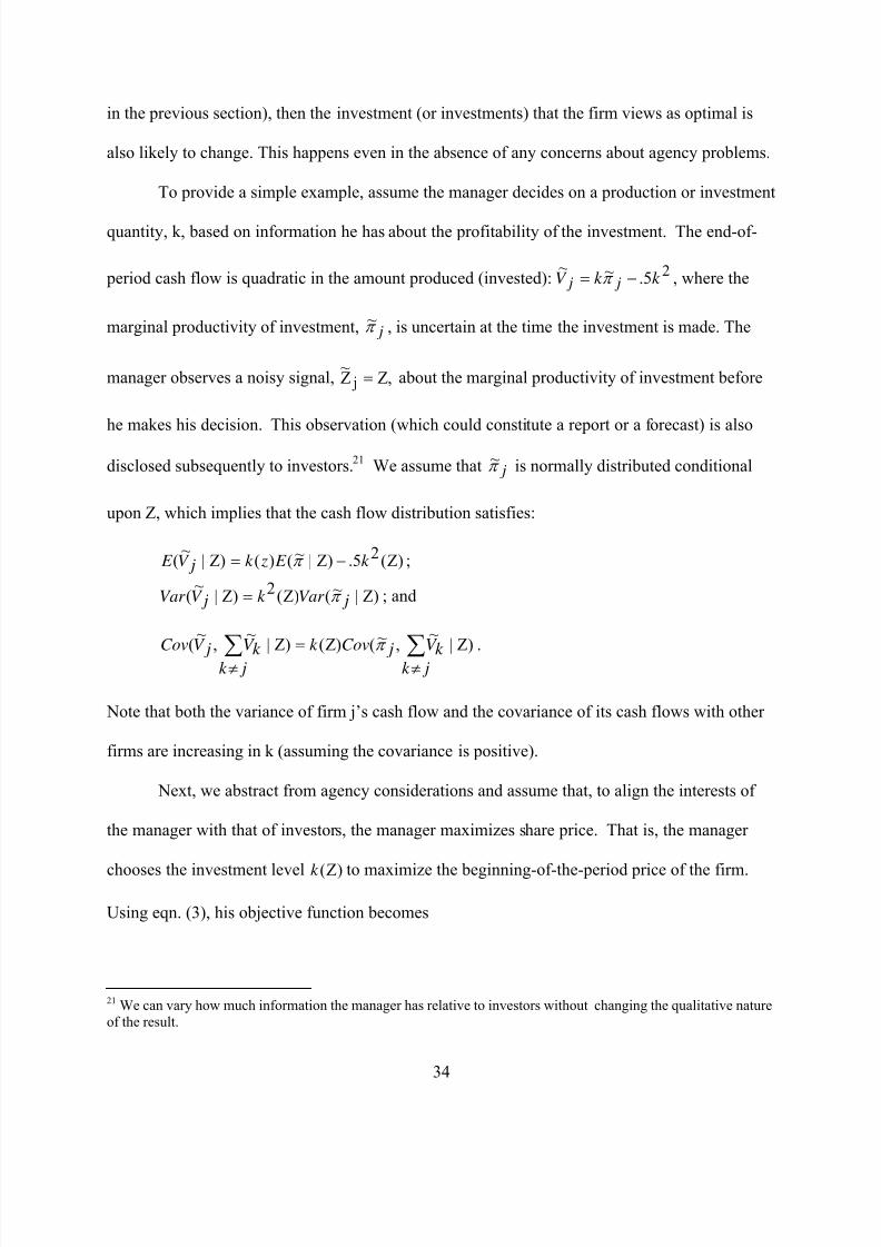
7/28/2019 Contabilitate si costul capitalului
http://slidepdf.com/reader/full/contabilitate-si-costul-capitalului 35/54
in the previous section), then the investment (or investments) that the firm views as optimal is
also likely to change. This happens even in the absence of any concerns about agency problems.
To provide a simple example, assume the manager decides on a production or investment
quantity, k, based on information he has about the profitability of the investment. The end-of-
period cash flow is quadratic in the amount produced (invested):2
5.~~k k V j j −= π , where the
marginal productivity of investment, jπ ~ , is uncertain at the time the investment is made. The
manager observes a noisy signal, ,ZZ~
j = about the marginal productivity of investment before
he makes his decision. This observation (which could constitute a report or a forecast) is also
disclosed subsequently to investors.21
We assume that jπ ~ is normally distributed conditional
upon Z, which implies that the cash flow distribution satisfies:
)Z(25.)Z|~()()Z|~
( k E zk jV E −= π ;
)Z|~()Z(2
)Z|~
( jVar k jV Var π = ; and
)Z|~
,~()Z()Z|~
,~
(
∑∑ ≠=
≠ jk k V
jCovk
jk k V
jV Cov π .
Note that both the variance of firm j’s cash flow and the covariance of its cash flows with other
firms are increasing in k (assuming the covariance is positive).
Next, we abstract from agency considerations and assume that, to align the interests of
the manager with that of investors, the manager maximizes share price. That is, the manager
chooses the investment level to maximize the beginning-of-the-period price of the firm.
Using eqn. (3), his objective function becomes
)Z(k
21 We can vary how much information the manager has relative to investors without changing the qualitative nature
of the result.
34
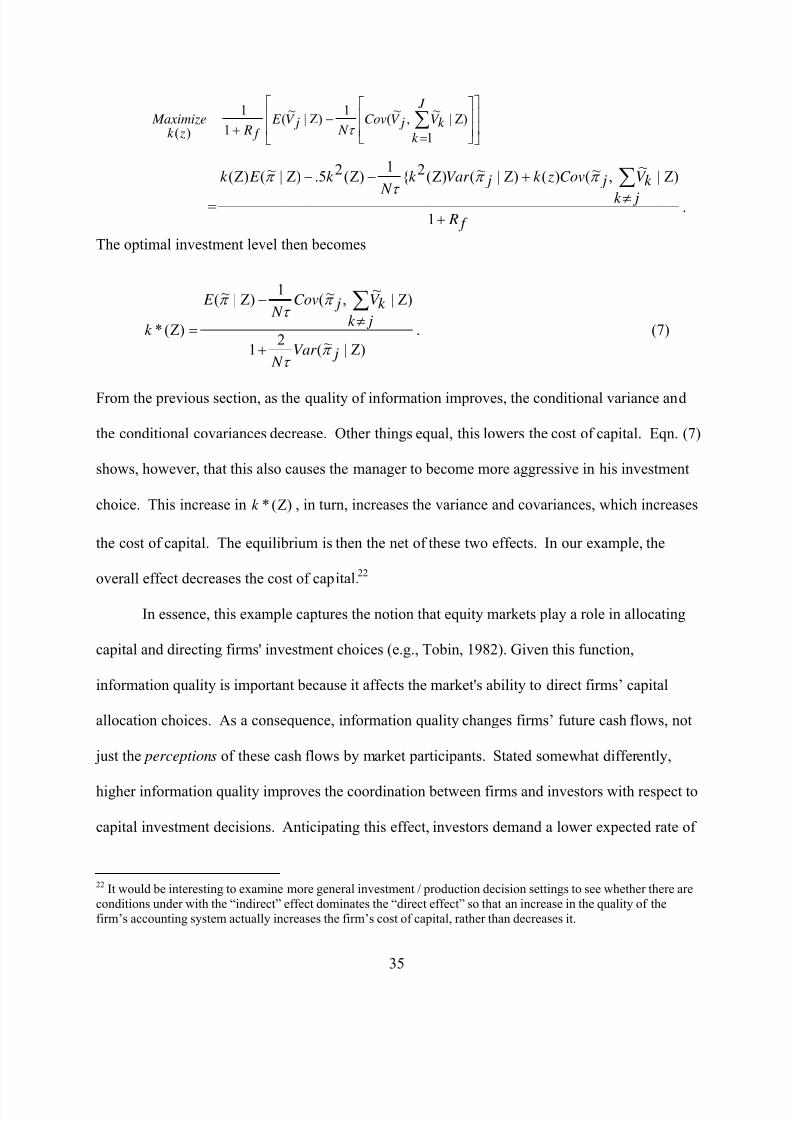
7/28/2019 Contabilitate si costul capitalului
http://slidepdf.com/reader/full/contabilitate-si-costul-capitalului 36/54
⎥⎥
⎦
⎤
⎢⎢
⎣
⎡
⎥⎥
⎦
⎤
⎢⎢
⎣
⎡
=−
+∑ )Z|
1
~,
~(
1)Z|
~(
1
1
)(
J
k
k V jV Cov N
jV E f R zk
Maximizeτ
= f R
jk
k V jCov zk jVar k
N
k E k
+≠
+−− ∑
1
)Z|~
,~()()Z|~()Z(2{1
)Z(25.)Z|~()Z( π π
τ
π
.
The optimal investment level then becomes
)Z|~(2
1
)Z|~
,~(1
)Z|~(
)Z(*
jVar N
jk
k V jCov N
E
k
π τ
π τ
π
+
≠−
=
∑. (7)
From the previous section, as the quality of information improves, the conditional variance and
the conditional covariances decrease. Other things equal, this lowers the cost of capital. Eqn. (7)
shows, however, that this also causes the manager to become more aggressive in his investment
choice. This increase in , in turn, increases the variance and covariances, which increases
the cost of capital. The equilibrium is then the net of these two effects. In our example, the
overall effect decreases the cost of capital.
)Z(*k
22
In essence, this example captures the notion that equity markets play a role in allocating
capital and directing firms' investment choices (e.g., Tobin, 1982). Given this function,
information quality is important because it affects the market's ability to direct firms’ capital
allocation choices. As a consequence, information quality changes firms’ future cash flows, not
just the perceptions of these cash flows by market participants. Stated somewhat differently,
higher information quality improves the coordination between firms and investors with respect to
capital investment decisions. Anticipating this effect, investors demand a lower expected rate of
22 It would be interesting to examine more general investment / production decision settings to see whether there are
conditions under with the “indirect” effect dominates the “direct effect” so that an increase in the quality of the
firm’s accounting system actually increases the firm’s cost of capital, rather than decreases it.
35
7/28/2019 Contabilitate si costul capitalului
http://slidepdf.com/reader/full/contabilitate-si-costul-capitalului 37/54
return. In short, investors price the risk of misalignment or misallocation that stems from poor
information quality.
When there are agency problems between firms and managers, the quality of the firm’s
accounting and information system also affects the magnitude of these agency problems, and
further changes the equilibrium production and investment decisions. Obviously, this involves
modeling and analyzing the incentive mechanisms used to motivate the manager and monitor his
decision. We leave this to future research to explore. It would be particularly interesting to
examine the interaction between firm-specific factors and cost of capital in such a setting. For
example, Christensen et al., (2002) examine how “idiosyncratic” risk affects managers’
investment decisions, and how compensation schemes should consider idiosyncratic and
nondiversifiable risks. Future research could explore how the cost of capital charged to
managers via compensation schemes influences their investment choices, and how this then
affects the cost of capital to shareholders.
As the discussion above suggests, a change in accounting and disclosure systems affects
the variances and covariances both directly and indirectly through real decisions. When a
change leads to a shift in both the expected value and the covariances, the overall impact on
cost of capital can be signed when the effects are reinforcing; that is, when expected cash flow
and the overall covariance with all firms’ cash flows move in opposite directions. When these
two factors move in the same direction, however, we cannot sign the overall impact without
placing more structure on the analysis. For example, we can sign the overall impact on the cost
of capital as long as the expected value does not change “too much” relative to the change in the
covariance. We formalize this notion in the next proposition.
36

7/28/2019 Contabilitate si costul capitalului
http://slidepdf.com/reader/full/contabilitate-si-costul-capitalului 38/54
Proposition 4. Let µ denote the expected cash flows and σ denote the covariance of the firm’s
cash flows with those of the market given an information system and the decision that results
from that information system. Let µ ′ be the change in µ that accompanies the change in σ.
Then the overall impact of a change in σ on the firm’s cost of capital has the same sign as the
term, µ σ
µ ′− .
For example, an increase in σ without any increase in µ results in an increase in the firm’s cost
of capital, just as in Proposition 1. Similarly, if σ increases while µ decreases, these effects
reinforce each other, and the cost of capital increases. When σ and µ change in the same
direction, Proposition 4 places a bound on the extent of the impact on µ. In particular, the impact
on µ cannot exceed the ratio of the mean to the covariance. Note that this ratio can also be
interpreted as the inverse of a measure analogous to the coefficient of variation of the cash flows,
except it is the contribution of the firm to the overall variance of the market, not its own variance
per se that is relevant.
An alternative way to state the condition in Proposition 4 is that the overall impact of a
change in σ on the cost of capital is positive (negative) if ⎥⎦
⎤⎢⎣
⎡σ
µ
σ ln
d
d is less than (greater than)
zero. For example, suppose that the expected value is related to the covariance through the
following functional form: σ ψ ψ µ 10 += , where ψ0 and ψ1 are arbitrary positive constants.
Then we can use Proposition 4 to show that an increase in σ leads to an increase in the cost of
capital, whereas a decrease in σ results in a decrease in the cost of capital.
37
7/28/2019 Contabilitate si costul capitalului
http://slidepdf.com/reader/full/contabilitate-si-costul-capitalului 39/54
5. Conclusion
In this paper, we develop a framework that links the disclosure of accounting information
to the cost of capital. Specifically, we examine whether and how the quality of a firm’s
accounting information manifests in its cost of capital, despite the forces of diversification. We
build a model of a multi-security economy that is consistent with the CAPM, but expressed in
terms of cash flows, rather than returns. We augment this model with an information structure
where accounting information and firms’ disclosure policies are represented as noisy information
about firms’ future cash flows.
Using this framework, we demonstrate that the quality of accounting information
influences a firm’s cost of capital, both directly by affecting market participants’ perceptions
about the distribution of future cash flows, and indirectly by affecting real decisions that alter the
distribution of future cash flows. The direct effect occurs because the quality of disclosures
affects the assessed covariances between a firm’s cash flow with other firms’ cash flows. This
effect is not diversifiable in large economies. Our finding provides a direct link between the
quality of a firm’s disclosures and accounting policies and its cost of capital. In addition, it
extends prior work in the estimation risk literature.
Our result that accounting information can lower a firm’s cost of capital contrasts with
contemporaneous work by Hughes et al. (2005). Their paper only analyzes the direct effect of
information, and concludes that only the market-wide risk premium changes; information has no
cross-sectional effect. One reason for the apparent contrast to our results is the different
definition of cost of capital. In particular, Hughes et al. define cost of capital as the difference
between beginning-of-period price and end-of-period expected cash flows, whereas we use the
more conventional definition of the expected rate of return on the firm’s stock. Once we
38
7/28/2019 Contabilitate si costul capitalului
http://slidepdf.com/reader/full/contabilitate-si-costul-capitalului 40/54
translate results from Hughes et al. into our definition of cost of capital, cross-sectional effects
on cost of capital manifest. The nature of the cross-sectional effects differs from ours, however,
due to the differences in the information structures assumed. Moreover, if indirect effects such
as those we consider were introduced into Hughes et al., there would be additional cross-
sectional differences in the effect of information on the cost of capital.
The indirect effect occurs because disclosure quality can change a firm’s real decisions.
As a consequence, the ratio of a firm’s expected future cash flows to the covariance of these cash
flows with the sum of all firms’ cash flows changes. This ratio is a key determinant of a firm’s
cost of capital. We show the indirect effect can go in either direction, but also derive conditions
under which an increase in information quality leads to an unambiguous decline in a firm’s cost
of capital.
These results have a number of important empirical implications, but they need to be
carefully interpreted. First, the direct and indirect effects that we discuss are entirely consistent
with the CAPM. That is, the information effects demonstrated in this paper are fully captured by
an appropriately specified forward-looking beta and the market-wide premium for risk.
Therefore, our model does not provide a theoretical justification for an “information risk” factor,
over and above beta. Empirical studies that are based on our results should therefore focus first
on the link between information quality and the beta factor. Alternatively, researchers could
appeal to the notion that empirical proxies for beta, which are based on historical returns, are
unlikely to capture all information effects on the forward-looking beta. But this justification is
different from one where additional variables are included in the empirical specification to
capture an “information risk” factor outside the one-factor CAPM. If they adopt this
justification, researchers should specify a “measurement error” model or, at least, provide careful
39

7/28/2019 Contabilitate si costul capitalului
http://slidepdf.com/reader/full/contabilitate-si-costul-capitalului 41/54
reasoning why and how the information variables help in capturing measurement error in the
forward-looking beta.
Second, empirical researchers should exercise care in interpreting our analysis of the
indirect effects of information quality. Our analysis takes place at the firm level, whereas
empirical studies are often conducted cross-sectionally for a number of firms. In a cross-
sectional setting, it is possible that the indirect effects will have different directional effects
across firms. Unless the researcher is careful to specify what decisions are affected and build
these directional predictions into the empirical analysis, the empirical analysis may mistakenly
conclude that there are no indirect effects. That is, the researcher will estimate the “average”
indirect effect, which could obscure positive indirect effects for some firms and negative indirect
effects for others. Moreover, empirical studies will generally measure the sum of the direct and
indirect effects of information quality.
Finally, we briefly comment on the impact of mandated disclosures or accounting
policies on firms’ cost of capital. Based on our model, increasing the quality of mandated
disclosures should generally reduce the cost of capital for each firm in the economy (assuming
that the expected cash flow of each firm and the covariance of that firm’s cash flow with the
market have the same sign). Nonetheless, disclosure regulation is likely to affect firms’ assessed
covariances with other firms differentially; hence, the benefits of mandatory disclosures are
likely to differ across firms. For example, mandated disclosure may reduce the covariance of
one firm’s cash flows with the sum of the cash flows of all firms faster than for other firms.
Because mandated disclosure impacts the covariances of all firms with each other, a
significant portion of its impact on the cost of capital of firms occurs through lowering the
market risk premium. The effect of mandated disclosure on firms’ beta factors is more difficult
40

7/28/2019 Contabilitate si costul capitalului
http://slidepdf.com/reader/full/contabilitate-si-costul-capitalului 42/54
to predict. In particular, mandated disclosure cannot lower the beta coefficients of all firms
because beta coefficients measure relative risk, and hence must aggregate to 1.0 regardless of the
information set available to investors. The betas of those firms whose covariances of cash flows
with the sum of the cash flows of all firms decrease relatively faster are likely to fall, while those
whose covariances decrease relatively slower are likely to rise. Therefore, while mandated
disclosure generally results in each firm having a lower cost of capital, its impact on betas is
ambiguous.
41

7/28/2019 Contabilitate si costul capitalului
http://slidepdf.com/reader/full/contabilitate-si-costul-capitalului 43/54
APPENDIX
Proof of equation (3).
Consider an economy with J firms, indexed by the subscript j = 1, 2,...,J , and a risk-
free bond. We assume that the risk-free rate of return is Rf ; that is, an investment
of $1 in the risk-free bond yields a return of $1 + Rf . Let V j and P j represent the
uncertain cash flows of firm j and the market equilibrium price of firm j, respectively.
Along with the J firms, we introduce a perfectly competitive market for firm shares
comprised of N investors, indexed by the subscript i = 1, 2,...,N , where N is large.
We represent investors’ (homogeneous) knowledge about firms’ cash flows by Φ.
Let U (c) represent investor i’s utility preference for an amount of cash c. Each
investor has a negative exponential utility function: that is, U (c) is defined by
U (c) = τ
µ1− exp
∙−
1
τ c
¸¶,
where τ > 0 describes each investor’s (constant) tolerance for risk. Note that this
characterization of the negative exponential has the feature that as risk tolerance
becomes unbounded, U (c) converges asymptotically to risk neutrality:
limτ →∞
U (c) = limτ →∞
τ
µ1− exp
∙−
1
τ c
¸¶→ c.
In addition, U (·) is standardized such that U (0) = 0.
Now consider the market price for firm j that prevails in a perfectly competitive
market in which N investors compete to hold shares in each firm, as well as a risk-free
bond. Let Di = {Di1, Di2,...,Dij,...,DiJ } represent the 1 × J vector of investor i’s
demand for ownership in J firms, where Dij represents investor i’s demand for firm j
expressed as percentage of the total firm; let D∗
i =n
D∗
i1, D∗
i2,...,D∗
ij,...,D∗
iJ
orepresent
her vector of endowed ownership in firms, where D∗
ij represents her endowment in
41

7/28/2019 Contabilitate si costul capitalului
http://slidepdf.com/reader/full/contabilitate-si-costul-capitalului 44/54
firm j expressed as a percentage of the total firm; and let P = {P 1, P 2,...,P j,...,P J }
represent the vector of firm prices, where once again P j represents the price of firm j.
Let Bi and B∗i
represent investor i’s demand for a risk-free bond and her endowment
in bonds, respectively. Each investor solves
maxDi,Bi
E [τ (1− exp[−1
τ (Di{V 1, V 2, ..., V J }
0 + (1 + Rf ) Bi)])|Φ] (A1)
subject to the budget constraint
DiP 0 + Bi = D∗
i P 0 + B∗i .
Taking the expectation of eqn. (A1) and substituting in the relation Bi = D∗
i P 0 +
B∗i − DiP 0 yields the following expression
maxDi,Bi
τ (1− exp[−1
τ (Di{E
hV 1|Φ
i− (1 + Rf ) P 1,
E h
V 2|Φi− (1 + Rf ) P 2,...,E
hV J |Φ
i− (1 + Rf ) P J }
0
+ (1 + Rf ) D∗
i P 0 + (1 + Rf ) B∗i ) +1
2
1
τ 2DiΛD0
i]), (A2)
where Λ is an J × J covariance matrix whose s, t-th term is Covh
V s · V t|Φi.
The first-order condition that maximizes eqn. (A2) with respect to Dij
reduces
to
0 = E h
V j|Φi− (1 + Rf ) P j −
1
τ
J Xk=1
DikCovh
V j · V k|Φi
. (A3)
Because collectively investors have claims to the cash flows of the entire firm, for each
k it must be the case thatPN
i=1 Dik = 1. Thus, summing over both sides of eqn. (A3)
with respect to i yields
0 = N ³E hV j|Φi− (1 + Rf ) P j´− 1
τ
N
Xi=1
J
Xk=1
DikCov hV j · V k|Φi ,
or
0 = N ³
E h
V j|Φi− (1 + Rf ) P j
´−
1
τ
J Xk=1
Covh
V j · V k|Φi
.
42

7/28/2019 Contabilitate si costul capitalului
http://slidepdf.com/reader/full/contabilitate-si-costul-capitalului 45/54
This, in turn, implies that the price for firm j is given by
P j =E h
V j|Φi−
1N τ
Covh
V j ·PJ
k=1 V k|Φi
1 + Rf
.
Q.E.D.
Proof of Proposition 1.
From Lemma 1,
E h
R j
i=
Rf H + 1
H − 1,
where
H =N τ E
hV j
iCov
hV j ,
PJ k=1 V k
i .
When
E h
V ji
> 0 and Cov
"V j,
J Xk=1
V k
#> 0,
H is increasing in both E h
V ji
and N τ , and decreasing in Covh
V j,PJ
k=1 V ki. Note
also that the derivative of E h
R j
iwith respect to H is negative:
∂ E h
R j
i∂ H
=(H − 1) Rf − (Rf H + 1)
(H − 1)2
=HRf −Rf −Rf H − 1
(H − 1)2
= −1 + Rf
(H − 1)2< 0.
Combining these, we have: E h
R j
iis decreasing in both E
hV ji
and N τ , and increasing
in Covh
V j,PJ
k=1 V ki. Finally, provided that H > 1, which is necessary for P j > 0, we
have E h
R j
iis increasing in Rf . Q.E.D.
Proof of Proposition 2.
We assume that V j , V k, ε j, and εk each have a normal distribution and define Z j and
Z k as Z j = V j + ε j and Z k = V k + εk. Our only additional distributional assumption
43

7/28/2019 Contabilitate si costul capitalului
http://slidepdf.com/reader/full/contabilitate-si-costul-capitalului 46/54
is that V j and V k are independent of ε j and εk, but not of each other. Taken together,
these assumptions imply that V j, V k, Z j , and Z k have a 4-variate normal distribution
with an unconditional covariance matrix given by
M =
⎡⎢⎢⎢⎢⎢⎢⎢⎢⎢⎣
V arh
V ji
Covh
V j, V ki
V arh
V ji
Covh
V j , V ki
Covh
V j, V ki
V arh
V ki
Covh
V j, V ki
V arh
V ki
V arh
V ji
Covh
V j, V ki
V arh
V ji
+ V ar [ε j] Covh
V j , V ki
+ Cov [ε j, εk]
Covh
V j, V ki
V arh
V ki
Covh
V j, V ki
+ Cov [ε j, εk] V arh
V ki
+ V ar [εk]
⎤⎥⎥⎥⎥⎥⎥⎥⎥⎥⎦
.
Simplify the covariance matrix notationally by setting: V = V arh
V ji; U = V ar
hV ki;
C = Cov hV j , V ki; e = V ar [ε j]; f = V ar [εk]; and c = Cov [ε j, εk]. This implies
M =
⎡⎢⎢⎢⎢⎢⎢⎢⎢⎢⎣
V C V C
C U C U
V C V + e C + c
C U C + c U + f
⎤⎥⎥⎥⎥⎥⎥⎥⎥⎥⎦
.
The inverse of M is
M −1 =
⎡⎢⎢⎢⎢⎢⎢⎢⎢⎢⎣
UV f +U ef −U c2−C 2f V Uef −V U c2−C 2ef +C 2c2
−Cef −C 2c−Cc2+U V c
V Uef −V U c2−C 2ef +C 2c2−
f ef −c2
cef −c2
−Cef −C 2c−Cc2+U V c
V Uef −V U c2−C 2ef +C 2c2V eU +V ef −V c2−C 2e
V Uef −V U c2−C 2ef +C 2c2c
ef −c2−
eef −c2
−f
ef −c2c
ef −c2f
ef −c2−
cef −c2
cef −c2
−e
ef −c2−
cef −c2
eef −c2
⎤⎥⎥⎥⎥⎥⎥⎥⎥⎥⎦
.
Let m describe the submatrix
m =
⎡⎢⎣
UV f +U ef −Uc2−C 2f V Uef −V U c2−C 2ef +C 2c2
−Cef −C 2c−Cc2+U V c
V Uef −V U c2−C 2ef +C 2c2
−Cef −C 2c−Cc2+U V c
V Uef −V U c2−C 2ef +C 2c2V eU +V ef −V c2−C 2e
V Uef −V U c2−C 2ef +C 2c2
⎤⎥⎦ .
Then the covariance matrix for V j and V k conditional on Z j and Z k is given by
m−1 =
⎡⎢⎣
V eU +V ef −V c2−C 2e
V U +V f +eU +ef −(C +c)2UV c+Cef −Cc(C +c)
V U +V f +eU +ef −(C +c)2
UV c+Cef −Cc(C +c)
V U +V f +eU +ef −(C +c)2UV f +Uef −U c2−C 2f
V U +V f +eU +ef −(C +c)2
⎤⎥⎦ .
44

7/28/2019 Contabilitate si costul capitalului
http://slidepdf.com/reader/full/contabilitate-si-costul-capitalului 47/54
The off -diagonal terms in m−1 describe Covh
V j, V k|Z j, Z ki: that is,
Covh
V j, V k|Z j, Z ki
=U V c + Cef − Cc (C + c)
V U + V f + eU + ef − (C + c)2. (A4)
Here we analyze the special case where only firm j provides information about its
cash flow: the proof to Corollary 1 (below) considers the case in which firms j and
k both report. Firm j alone providing information is (mathematically) equivalent
to the measurement error in firm k’s information about its cash flow, f = V ar [εk],
becoming unboundedly large (i.e., f → ∞). In this case, the conditional covariance
reduces to
Covh˜
V j ,˜V k|Z j
i= limf →∞Cov
h ˜V j,
˜V k|Z j , Z k
i→ C
e
V + e
= Covh
V j, V ki V ar [ε j ]
V arh
V ji
+ V ar [ε j].
This expression clearly shows that a reduction in firm j’s measurement error attenu-
ates the unconditional covariance. In fact, measurement error in the variance in j’s
information determines the percentage of attenuation. Q.E.D.
Corollary to Proposition 2: An Extension to Disclosure by Two Firms.
Recall that from the proof of Proposition 2 the covariance of the cash flows of firms
j and k, V j and V k, conditional on each firm disclosing information about their re-
spective cash flows, Z j and Z k, is
Covh
V j, V k|Z j, Z ki
=U V c + Cef − Cc (C + c)
V U + V f + eU + ef − (C + c)2. (A4)
Re-expressing the conditional covariance in terms of (exclusively) standard deviations
and correlations yields
Covh
V j, V k|Z j, Z ki
= vurvu (1− r2) ρ
rεφ + ε2φ2 (1− ρ2)
v2u2 (1− r2) + (vφ− uε)2 + 2vuεφ (1− rρ) + ε2φ2 (1− ρ2),
(A5)
45

7/28/2019 Contabilitate si costul capitalului
http://slidepdf.com/reader/full/contabilitate-si-costul-capitalului 48/54
where V = v2, U = u2, C = vur, e = ε2, f = φ2, and c = εφρ. This implies that
the correlation in the cash flows of firms j and k is r, and the correlation in their
disclosure errors about those cash flows, ε j and εk respectively, is ρ. Next, calculate
the derivative of Covh
V j, V k|Z j, Z ki
with respect to the standard deviation in the
disclosure error in Z j , ε, and evaluate the derivative in a circumstance in which firms
j and k are “otherwise identical”: that is, the standard deviations in their respective
cash flows and disclosure errors are identical (i.e., v = u and ε = φ). In other words,
calculate∂
∂εCov
hV j , V k|Z j, Z k
i|v=u,ε=φ.
Note that this calculation requires that one first compute ∂ ∂ε
Covh
V j, V k|Z j, Z ki
and
then evaluate this expression at v = u and ε = φ: this is tantamount to a change in
firm j’s disclosure error holding firm k’s disclosure error fixed. It is a straightforward
exercise to show that the sign of ∂ ∂ε
Covh
V j, V k|Z j , Z ki|v=u,ε=φ is determined by the
sign of the expression
ρ (1 + r)2 (1− r)2 v4 + 2r ³1− ρ2´ ³1− r2´ v2ε2
+³
1− ρ2´
(r (1− rρ) + (r − ρ)) ε4. (A6)
The sign of the first term in eqn. (A6) is determined by the sign of the correlation
in disclosure errors, ρ; the sign of the second term is determined by the sign of the
correlation in cash flows, r; and the sign of the third term is determined by the sign
of the correlation in cash flows provided that the correlation is no less in magnitude
than the correlation in disclosure errors: that is, |r| ≥ |ρ|. Thus, assume that the
correlations in cash flows and disclosure errors do not have opposite signs, and the
magnitude of the former is no less than that of the latter. Then, if the unconditional
covariance in cash flows is non-negative (i.e., C = vur ≥ 0, which requires r ≥ 0),
46

7/28/2019 Contabilitate si costul capitalului
http://slidepdf.com/reader/full/contabilitate-si-costul-capitalului 49/54
then the conditional covariance in cash flows moves closer to 0 as the error in firm j’s
disclosure about its cash flow decreases (i.e., ∂ ∂ε
Covh
V j, V k|Z j, Z ki|v=u,ε=φ decreases
as ε decreases). Similarly, if the unconditional covariance in cash flows is negative
(i.e., C = vur < 0, which requires r < 0), then the conditional covariance in cash
flows moves closer to 0 as the error in firm j’s disclosure about its cash flow decreases
(i.e., ∂ ∂ε
Covh
V j , V k|Z j, Z ki|v=u,ε=φ increases as ε decreases). Thus, irrespective of
the sign of the unconditional covariance in cash flows, the conditional covariance in
cash flows moves closer to 0 as the error in firm j’s disclosures about its cash flow
decreases. Finally, note that when disclosure errors are uncorrelated, i.e., ρ = 0, then
the correlations in cash flows and disclosure errors do not have opposite signs, and
the magnitude of the former is no less than that of the latter. Thus, in the special
case of uncorrelated disclosure errors, the conditional covariance in cash flows moves
closer to 0 as the error in firm j’s disclosures about its cash flow decreases. Q.E.D.
Proof of Proposition 3.
The expected value and covariance of the net amount received by the firm’s share-
holders areE h
V j|Qi
= (1 −A1 (Q)) E h
V ∗ j
i−A0 (Q) ,
and
1
N τ Cov
"V j,
J Xk=1
V k|Q
#=
1
N τ
⎛⎝[1− A1 (Q)]2 V ar
hV ∗ j
i+ [1−A1 (Q)] Cov
⎡⎣V j,
J Xk6= j
V k|Q
⎤⎦⎞⎠ ,
respectively, where A1 (Q) is between 0 and 1. With a large number of firms, the
firm-variance eff ect is small; thus, H (Q) can be expressed as
H (Q) =E h
V j|Qi
1N τ
Covh
V j ,PJ
k=1 V k|Qi ≈ (1− A1 (Q)) E
hV ∗ j
i−A0 (Q)
(1−A1 (Q)) Covh
V j,PJ
k6= j V k|Qi .
47

7/28/2019 Contabilitate si costul capitalului
http://slidepdf.com/reader/full/contabilitate-si-costul-capitalului 50/54
Next, for convenience let E ∗ and C ∗ represent E h
V ∗ j
iand Cov
hV j ,
PJ k6= j V k|Q
i, re-
spectively. Then
∂ H ∂ Q
= (−A
0
1 (Q) E
∗
−A
0
0 (Q))(1−A1 (Q)) C
∗
− ([1−A1 (Q)] E
∗
−A0 (Q)) (−A
0
1 (Q) C
∗
)([1−A1 (Q)] C ∗)2
=−A0
0 (Q) (1−A1 (Q)) C ∗ −A0 (Q) A01 (Q) C ∗
([1−A1 (Q)] C ∗)2
=−A0
0 (Q) (1−A1 (Q))−A0 (Q) A01 (Q)
(1−A1 (Q))2 C ∗.
Noting that A00 (Q) and A0
1 (Q) are both non-positive, provided that A0 (Q) is non-
negative and C ∗ > 0 we have∂ H
∂ Q ≥ 0;
if C ∗ < 0 the reverse result holds, and if A0 (Q) = A00 (Q) = 0 then ∂ H
∂ Q= 0. Finally,
from Lemma 1 the cost of capital is decreasing in H (Q). Q.E.D.
Proof of Proposition 4.
Cost of capital is defined as
E hR j|Φi =Rf E
hV j |Φ|
i+ 1
N τ Cov
hV j,
PJ k=1 V k |Φ|
i
E h ˜
V j |Φ|i−
1
N τ Covh˜
V j,PJ
k=1
˜V k |
Φ|i .
Let σ = Covh
V j ,PJ
k=1 V k |Φ|i, µ = E
hV j |Φ|
i, and µ0 = ∂
∂ Cov[V j ,PJ
k=1V k|Φ|]
E h
V j |Φ|i.
This allows E h
R j|Φi
to be defined as
E h
R j|Φi
=Rf µ + 1
N τ σ
µ− 1N τ
σ.
In addition,
∂
∂σ E h
R j|Φi
=³Rf µ
0 + 1N τ ´ ³µ− 1
N τ σ´− ³Rf µ + 1
N τ σ´ ³µ0 − 1
N τ ´³µ− 1
N τ σ´2
= −
1N τ
(σµ0 − µ) (Rf + 1)³µ− 1
N τ σ´2 .
48

7/28/2019 Contabilitate si costul capitalului
http://slidepdf.com/reader/full/contabilitate-si-costul-capitalului 51/54
This implies that ∂ ∂σ
E h
R j|Φi
assumes the same sign as the sign of the change in σ
provided that
µ0 <µ
σ.
In other words, a decrease in σ implies a decrease in E h
R j|Φi, provided that µ0 < µ
σ.
Q.E.D.
49

7/28/2019 Contabilitate si costul capitalului
http://slidepdf.com/reader/full/contabilitate-si-costul-capitalului 52/54
REFERENCES
Admati, A., P. Pfleiderer, 2000, Forcing firms to talk: financial disclosure regulation and
externalities, The Review of Financial Studies 13, 479-519.
Amihud, Y., H. Mendelson, 1986, Asset pricing and the bid-ask spread, Journal of Financial
Economics 17, 223-249.
Ashbaugh-Skaife, H., Collins, D., Kinney, W., and R. LaFond, 2005, “The Effect of Internal
Control Deficiencies on Firm Risk and Cost of Equity Capital,” working paper,
University of Iowa.
Baiman, S., R. Verrecchia, 1996, The relation among capital markets, financial disclosure, production efficiency, and insider trading, Journal of Accounting Research 34, 1-22.
Barry, C., S. Brown, 1984, Differential information and the small firm effect, Journal of
Financial Economics 13, 283-294.
Barry, C., S. Brown, 1985, Differential information ad security market equilibrium, Journal of
Financial and Quantitative Analysis 20, 407-422.
Beaver, W., P. Kettler, M. Scholes, 1970, The association between market-determined andaccounting-determined measures of risk, The Accounting Review 45, 654-682.
Berger, P., Chen, H., and F. Li, 2005, “Firm Specific Information and Cost of Equity, working
paper, University of Chicago.Bhoraj, S., C. M. C. Lee, and D. Oler. 2003. What’s my line? A comparison of industry
classification schemes for capital market research. Journal of Accounting Research 41:
745-774.
Botosan, C., 1997, Disclosure level and the cost of equity capital, The Accounting Review 72,323-349.
Botosan, C., M. Plumlee, 2002, A re-examination of disclosure level and the expected cost of equity capital, Journal of Accounting Research 40, 21-41.
Brown, S., 1979, The effect of estimation risk on capital market equilibrium, Journal of
Financial and Quantitative Analysis 15, 215-220.
Brown, P., and R. Ball. 1967. Some preliminary findings on the association between the earnings
of a firm, its industry, and the economy. Journal of Accounting Research 5: 55-77.
Chordia, T., R. Roll, A. Subrahmanyam, 2001, Market liquidity and trading activity, Journal of
Finance 56, 501-530.
Christensen, P., G. Feltham, M. Wu, 2002, ‘Cost of capital’ in residual income for performance
evaluation, The Accounting Review 77, 1-23.
Coles, J., U. Loewenstein, 1988, Equilibrium pricing and portfolio composition in the presenceof uncertain parameters, Journal of Financial Economics 22, 279-303.
Coles, J., U. Loewenstein, J. Suay, 1995, On equilibrium pricing under parameter uncertainty,
The Journal of Financial and Quantitative Analysis 30, 347-374.
50

7/28/2019 Contabilitate si costul capitalului
http://slidepdf.com/reader/full/contabilitate-si-costul-capitalului 53/54
Core, J., W. Guay, R. Verdi, 2006, Is Accruals Quality a Priced Risk Factor?, Working paper,
University of Pennsylvania.
Degroot, M., 1970, Optimal Statistical Decisions, Wiley and Sons, Hoboken NJ.
Diamond, D., R. Verrecchia, 1991, Disclosure, liquidity and the cost of capital, Journal of
Finance 46, 1325-1359.
Dye, R., 1990, “Mandatory Versus Voluntary Disclosures: The Case of Financial and Real
Externalities,” The Accounting Review, Vol. 65, No 1 ( January 1990), 1-24.
Easley, D., M. O’Hara, 2004, Information and the cost of capital, Journal of Finance 59, 1553-1583.
Easley, D., S. Hvidkjaer, M. O’Hara, 2002, Is information risk a determinant of asset returns?
Journal of Finance 57, 2185-2222.
Fama, E., 1976, Foundations of Finance, Basic Books, New York.
Fama, E., M. Miller, 1972, The Theory of Finance, Dryden Press, Hinsdale IL.
Fishman, M., K. Hagerty, 1989, Disclosure decisions by firms and the competition for priceefficiency, Journal of Finance 44, 633-646.
Foster, G., 1981, Intra-industry information transfers associated with earnings releases, Journal
of Accounting and Economics 3, 201-232.
Foster, N., 2003, The FASB and the capital markets, The FASB Report (June 2003).
Francis, J., R. LaFond, P. Olsson, K. Schipper, 2004, Costs of equity and earnings attributes, The
Accounting Review 79, 967-1010.
Freeman, R., and S. Tse. 1992. An earnings prediction approach to examining intercompany
information transfers. Journal of Accounting and Economics 15: 509-523
Gebhardt, W., C. Lee, C., B. Swaninathan, 2001, Toward an implied cost of capital, Journal of Accounting Research 39, 135-176.
Hail, L., C. Leuz, 2006, International differences in the cost of equity capital: do legalinstitutions and securities regulation matter? Journal of Accounting Research 44,
forthcoming.
Han, J., and J. Wild. 1990. Unexpected earnings and intra-industry information transfers: Further evidence. Journal of Accounting Research 28: 211-219.
Hughes, J., J. Liu, J. Liu, 2005, Information, diversification and the cost of capital, working paper, UCLA.
Kalymon, B., 1971, Estimation risk in the portfolio selection model, Journal of Financial and
Quantitative Analysis 6, 559-582.
Kanodia, C., A. Mukherji, H. Sapra, R. Venugopalan, 2000, Hedge disclosures, future prices,
and production distortions, Journal of Accounting Research 38, 53-83.
Kanodia, C., H. Sapra, R. Venugopalan, 2004, Should intangibles be measured: what are the
economic trade-offs? Journal of Accounting Research 42, 89-120.
51
7/28/2019 Contabilitate si costul capitalului
http://slidepdf.com/reader/full/contabilitate-si-costul-capitalului 54/54
Lambert, R., 2001, Contracting theory and accounting, Journal of Accounting and Economics
32, 3-87.
Lambert, R., C. Leuz, R. Verrecchia, 2006, The Distribution of Information Across Investors andthe Cost of Capital, Working paper, University of Pennsylvania.
La Porta, R., Lopez-de-Silanes, F., Shleifer, A., R. Vishny, 1997, Legal determinants of external
finance, Journal of Finance 52, 1131-1150.
Levitt, A., 1998, The importance of high quality accounting standards, Accounting Horizons 12,79-82.
Lintner, J., 1965, The Valuation of risk assets and the selection of risky investments in stock
portfolios and capital budgets, Review of Economics & Statistics 65, 13-37.
Lombardo, D., M. Pagano, 2002, Law and equity markets: a simple model, CSEF Working Paper
No. 25, and CEPR Discussion Paper No. 2276, in Corporate Governance Regimes:
Convergence and Diversity, J. McCahery, P. Moerland, T. Raaijmakers and L.
Renneboog (eds.), Oxford University Press, 343-362.
Merton, R., 1987, A simple model of capital market equilibrium with incomplete information, Journal of Finance 43, 483-510.
Pastor, L., R. Stambaugh, 2003, Liquidity risk and expected stock returns, Journal of Political
Economy 111, 642-685.
Piotroski, J., D. Roulstone, 2004, The influence of analysts, institutional investors and insiders
on the incorporation of market, industry and firm-specific information into stock prices,
The Accounting Review 79, 1119-1151.
Sharpe, W., 1964, Capital asset prices, a theory of market equilibrium under conditions of risk, Journal of Finance 19, 425-442.
Tobin, J., 1982, On the efficiency of the financial system, Lloyd's Banking Review 153, 1-15.Verrecchia, R., 1983, Discretionary disclosure, Journal of Accounting and Economics 5, p. 179-
194.
Verrecchia, R., 2001, Essays on disclosure, Journal of Accounting and Economic s 32, 97-180.