Consumption-Based AssetPricing Models

Rajnish Mehra1,2,3

1Department of Economics and Finance, Arizona State University,

Tempe, Arizona 85287; email: Rajnish.Mehra@asu.edu

2Luxembourg School of Finance, University of Luxembourg, L-1468 Luxembourg

3National Bureau of Economic Research, Cambridge, Massachusetts 02138

Annu. Rev. Financ. Econ. 2012. 4:385–409

The Annual Review of Financial Economics is

online at financial.annualreviews.org

This article’s doi:

10.1146/annurev-financial-102710-144825

Copyright © 2012 by Annual Reviews.

All rights reserved

JEL: D31, E2, E21, E44, G1, G11, G12, G23,

H0, H62

1941-1367/12/1205-0385$20.00

Keywords

equity premium puzzle, life cycle, borrowing constraints, retirement

Abstract

A major research initiative in finance focuses on the determinants

of the cross-sectional and time series properties of asset returns.

With that objective in mind, asset pricing models have been devel-

oped, starting with the capital asset pricing models of Sharpe (1964),

Lintner (1965), andMossin (1966). Consumption-based asset pricing

models use marginal rates of substitution to determine the relative

prices of the date, event-contingent, composite consumption good.

This model class is characterized by a stochastic discount factor

process that puts restrictions on the joint process of asset returns

and per capita consumption. This review takes a critical look at this

class of models and their inability to rationalize the statistics that

have characterized US financial markets over the past century.

The intuition behind the discrepancy between model prediction and

empirical data is explained. Finally, the research efforts to enhance

the model’s ability to replicate the empirical data are summarized.

385

Ann

u. R

ev. F

in. E

con.

201

2.4:

385-

409.

Dow

nloa

ded

from

ww

w.a

nnua

lrev

iew

s.or

gby

212

.76.

252.

243

on 1

1/05

/12.

For

per

sona

l use

onl

y.

1. INTRODUCTION

Amajor research initiative in finance focuses on the determinants of the cross-sectional and

time series properties of asset returns. With that objective in mind, asset pricing models

have been developed, starting with the capital asset pricing models of Sharpe (1964),

Lintner (1965), and Mossin (1966).

An asset pricing model is characterized by an operator that maps the sequence of future

random payoffs of an asset to a scalar, the current price of the asset.1 If the law of one

price2 holds in a securities market where trading occurs at discrete points in time, this

operator C .ð Þ can be represented as3

pt ¼ C fysg1s¼tþ1

� � ¼ E ½X1s¼tþ1

ms,t ys j Ft�, ð1Þ

where pt is the price at time t of an asset with stochastic payoffs fysg1s¼tþ1, fms,tg1s¼tþ1 is a

stochastic process,4 Ft is the information available to households who trade assets at

time t, and E is the expectations operator defined over random variables that are mea-

surable with respect to the sigma algebra generated by Ft. If the asset payoffs end at a

finite future time T, we define the random variables fysg1s¼Tþ1 to be zero. If the securities

market is arbitrage free,5 then the process fms,tg1s¼tþ1 has strictly positive support (with

probability one) and is unique if the market is complete.6

No arbitrage is a necessary condition for the existence of security market equilibrium

in an economy where all agents have access to the same information set. If, however,

there is an agent in the economy with preferences that can be represented by a strictly

increasing, continuous utility function defined over security payoffs, then no arbitrage is

both necessary and sufficient for the existence of a security market equilibrium7 (Dybvig &

Ross 2008). In an economy characterized by such an agent and no arbitrage, all equilib-

rium asset pricing models are simply versions of Equation 1 for different stochastic pro-

cesses fms,tg1s¼tþ1, often referred to as stochastic discount factors or pricing kernels.

Consumption-based asset pricing models use marginal rates of substitution to deter-

mine the relative prices of the date, event-contingent, composite consumption good.8 This

model class is characterized by a stochastic discount factor process that puts restrictions

on the joint process of asset returns and per capita consumption. The deus ex machina of

consumption-based asset pricing models is that, for a given endowment process, house-

hold trading of financial assets is motivated by a desire to smooth consumption both over

1Both the payoffs and the price are denominated in the numeraire consumption good.

2Assets that have identical payoffs have identical prices.

3See Ross (1976), Harrison & Kreps (1979), and Hansen & Richard (1987) for the technical restrictions on the

payoff process for Equation 1 to hold.

4ms,t ¼Ys�t�1

k¼0

mtþkþ1,tþk, where mtþkþ1,tþk is a random variable such that ptþk ¼ E ½mtþkþ1,tþk ytþkþ1 j Ftþk �.5A securities market is arbitrage free if no security is a free lottery and any portfolio of securities with a zero payoff

has a zero price.

6If markets are incomplete, there will, in general, be multiple processes fms,tg1s¼tþ1 such that Equation 1 holds.

Not all of them need have a strictly positive support.

7Households maximize utility given their endowments and security prices, and supply equals demand at these

security prices.

8In contrast, production-based asset pricing models use the marginal rates of transformation.

386 Mehra

Ann

u. R

ev. F

in. E

con.

201

2.4:

385-

409.

Dow

nloa

ded

from

ww

w.a

nnua

lrev

iew

s.or

gby

212

.76.

252.

243

on 1

1/05

/12.

For

per

sona

l use

onl

y.

time and across states at a point in time. The desirability of an asset in this model reflects

its ability to smooth consumption. Hence, assets that pay off in future states when con-

sumption levels are high—when the marginal utility of consumption is low—are less

desirable than those that pay an equivalent amount in future states when consumption

levels are low and additional consumption is more highly valued.9 As a consequence, the

price of a claim to a unit of consumption at some future time t scales in proportion to the

marginal utility of consumption at that time. Both the household’s elasticity of inter-

temporal substitution and risk aversion play a crucial role in this class of models.

In these models, ms,t is usually expressed as a function of the marginal rate of substitu-

tion of consumption between time s and t of the agents who trade securities. For example,

in a widely cited and influential paper, Lucas (1978) models ms,t as bs�tu0 csð Þ = u0 ctð Þ.Here ct is the aggregate per capita consumption at time t, u0 ctð Þ is the marginal utility

of consumption at time t, and b is the rate of time preference. In the case of constant

relative risk aversion (CRRA) preferences, this specializes to bs�t cs = ctð Þ�a, where a is

the coefficient of relative risk aversion and, simultaneously, the reciprocal of the elas-

ticity of intertemporal substitution. I make this precise in the discussion that follows in

Section 2.

In this review, I develop a consumption-based asset pricing model along the lines of

Lucas (1978). I next discuss the results in Mehra & Prescott (1985) that led to the equity

premium puzzle. Finally, I review the literature spanning almost thirty years that attempts

to resolve the puzzle.

2. A CONSUMPTION-BASED ASSET PRICING MODELWITHSTANDARD PREFERENCES

Actual asset prices are formed via the trading behavior of large numbers of heterogeneous

investors as each attempts to smooth consumption, given his information on the future

distribution of asset returns. Equilibria in such economies are difficult to characterize.

If financial markets are competitive and complete, and agent preferences satisfy

the von Neumann-Morgenstern axioms for expected utility, there will, in general,

exist, by construction, a representative (single-agent) economy with the same aggre-

gate consumption series as the heterogeneous-agent economy and the same asset price

functions. These economies are comparatively easy to analyze. In addition, if the repre-

sentative agent can be constructed in a manner that is independent of the underlying

heterogeneous-agent economy’s initial wealth distribution, we say that the economy

displays aggregation.

Aggregation (vis-a-vis the existence of a representative agent) is a stronger, more restrictive,

and more desirable property. It implies that assets may be priced in the representative-agent

economy without knowledge of the wealth distribution in the underlying heterogeneous-

agent counterpart. Under aggregation, results derived in the representative-agent economy

are general and robust. Aggregation also permits the use of the representative agent for

welfare comparisons.10

9Consumption levels are relative to current consumption.

10Suppose, alternatively, that aggregation fails. Then each possible initial wealth distribution, via its associated

representative agent, will display its own asset pricing characteristics. No general statements may be made unless

the market is complete.

www.annualreviews.org � Consumption-Based Asset Pricing Models 387

Ann

u. R

ev. F

in. E

con.

201

2.4:

385-

409.

Dow

nloa

ded

from

ww

w.a

nnua

lrev

iew

s.or

gby

212

.76.

252.

243

on 1

1/05

/12.

For

per

sona

l use

onl

y.

In the analysis to follow I assume a market structure that enables us to use the

representative-agent construct. In Section 3, I further restrict the utility function to be of

the constant relative risk aversion (CRRA) class

u c,að Þ ¼ c1�a

1� a, 0 < a < 1, ð2Þ

where the parameter a measures the curvature of the utility function. When a ¼ 1, the

utility function is defined to be logarithmic, which is the limit of the above representation

as a approaches 1.

The CRRA preference class has three attractive features that make it the preference

function of choice in much of the literature in growth and dynamic stochastic general

equilibrium macroeconomic theory. It allows for aggregation and time-consistent plan-

ning, and is scale invariant. I have discussed aggregation above. I examine the other two

features below.

Scale invariance means that a household is equally likely to accept a gamble if both

its wealth and the gamble amount are scaled by a positive factor. Hence, although the levels

of aggregate variables, such as the capital stock, stock prices, and aggregate dividends,

have increased over time, the resulting equilibrium return process with this preference

class is stationary. This is consistent with the statistical evidence on the time series of

asset returns over the past 100 years, which confirms that asset returns are stationary.

Any serious preference structure should yield equilibrium return series with this feature.

Time-consistent planning implies that optimal future-contingent portfolio decisions

made at t ¼ 0 remain the optimal decisions even as uncertainty resolves and intermediate

consumption is experienced. When considering multiperiod decision problems, time con-

sistency is a natural property to propose. In its absence, one would observe portfolio

rebalancing not motivated by any event or information flow but rather simply moti-

vated by the (unobservable) changes in the investor’s preference ordering as time passed.

Asset trades would be motivated by endogenous and unobservable preference characteris-

tics, and would thus be mysterious and unexplainable.

One disadvantage of this representation is that it links risk preferences with time

preferences. With CRRA preferences, agents who like to smooth consumption across

various states of nature also prefer to smooth consumption over time; that is, they dislike

growth. Specifically, the coefficient of relative risk aversion is the reciprocal of the elasticity

of intertemporal substitution. There is no fundamental economic reason why this must be.

In Section 4, I examine the asset pricing implications of alternate preference functions

where this restriction is relaxed.

I next consider the asset pricing characteristics of a frictionless economy that has a

single representative stand-in household with the above characteristics. This unit orders

its preferences over random consumption paths by

EX1t¼0

btu ctð Þ j F0

( ), 0 < b < 1, ð3Þ

where ct is the per capita consumption; u: Rþ ! R is a strictly increasing, continuously

differentiable concave utility function; and the parameter b is the subjective time discount

factor, which describes how impatient households are to consume. If b is small, people

are highly impatient, with a strong preference for consumption now versus consumption

388 Mehra

Ann

u. R

ev. F

in. E

con.

201

2.4:

385-

409.

Dow

nloa

ded

from

ww

w.a

nnua

lrev

iew

s.or

gby

212

.76.

252.

243

on 1

1/05

/12.

For

per

sona

l use

onl

y.

in the future. As modeled, these households live forever, which implicitly means that the

utility of parents depends on the utility of their children (see Becker & Barro 1988).

We assume one productive unit, which produces output yt in period t, which is the

period dividend. There is one equity share11 with price pt that is competitively traded;

it is a claim to the stochastic process fysg1s¼tþ1. To connect these concepts to the data, the

price pt will correspond to the value of the market portfolio and yt to the associated

aggregate dividend process. In the background is a more elaborate macroeconomic

model describing the origins of the fysg1s¼tþ1 sequence.12 Consider the intertemporal choice

problem of a typical investor at time t. He equates the loss in utility associated with

buying one additional unit of equity to the discounted expected utility of the resulting

additional consumption in the next period. To carry over one additional unit of equity

pt, units of the consumption good must be sacrificed, and the resulting loss in utility is

ptu0 ctð Þ. By selling this additional unit of equity in the next period, ptþ1 þ ytþ1, additional

units of the consumption good can be consumed, and bEtf(ptþ1 þ ytþ1)u0(ctþ1)g is the

discounted expected value of the incremental utility in the next period. At an optimum,

these quantities must be equal. This leads to the fundamental equation of consumption-

based asset pricing:

pt ¼ bEu0 ctþ1ð Þu0 ctð Þ ptþ1 þ ytþ1ð Þ j Ft

� �. ð4Þ

Equation 4 holds for any financial asset—stocks, bonds, or options.

Versions of this expression can be found in Rubinstein (1976), Lucas (1978), Breeden

(1979), and Donaldson & Mehra (1984), among others. Excellent textbook treatments

or surveys can be found in Campbell (2003), Cochrane (2005), Constantinides (2005),

Danthine & Donaldson (2005), Duffie (2001), and LeRoy & Werner (2001).

The recursive substitution of Equation 4 yields

pt ¼ EX1s¼tþ1

bs�t u0 csð Þ

u0 ctð Þ ys j Ft

( ). ð5Þ

This is identical to Equation 1, with a strictly positive ms,t equal to bs�tu0 csð Þ = u0 ctð Þ. If we

interpret the random variable ms,t as a discount factor, we see that the price of an asset

at time t is the expected discounted value of future payoffs.13

To gain additional intuition, we rewrite Equation 4 in terms of asset returns as14

Et Re,tþ1

� � ¼ Rf ,tþ1 þ Covt�U 0 ctþ1ð Þ,Re,tþ1

Et U0 ctþ1ð Þð Þ

� �. ð6Þ

Et is the expectation conditional on the information at time t,

Re,tþ1 ¼ ptþ1 þ ytþ1

pt

11We assume that the supply of shares is fixed.

12An implicit assumption is that the equity owners have no income source other than dividends.

13In a more elaborate model, such as Donaldson & Mehra (1984), the objective of the firm is to choose capital and

labor to maximize pt.

14This equation also holds unconditionally, a fact that I use when quantitatively evaluating the model in Section 3.

www.annualreviews.org � Consumption-Based Asset Pricing Models 389

Ann

u. R

ev. F

in. E

con.

201

2.4:

385-

409.

Dow

nloa

ded

from

ww

w.a

nnua

lrev

iew

s.or

gby

212

.76.

252.

243

on 1

1/05

/12.

For

per

sona

l use

onl

y.

is the gross return on equity, and

Rf ,tþ1 ¼ 1

qtð7Þ

is the gross rate of return on a one-period riskless bond with price qt:

qt ¼ bEtu0 ctþ1ð Þu0 ctð Þ

� �. ð8Þ

Expected asset returns equal the risk-free rate plus a premium for bearing risk, which

depends on the covariance of the asset returns with the marginal utility of consumption.

Hence, assets that covary positively with consumption—that is, they pay off in states when

consumption is high and marginal utility is low—command a high premium, given that

these assets destabilize consumption.

3. A QUANTITATIVE EVALUATION OF THE MODEL

To quantitatively evaluate the consumption-based asset pricing model developed above,

Mehra & Prescott (1985) computed the risk premium implied by the unconditional version

of Equation 6.15 They used the historical average return on the S&P 500 index as a proxy

for the expected return on the risky capital stock of the economy and the historical

average return on Treasury bills (T-bills) as a proxy for the risk-free rate. To their surprise,

they found the maximum risk premium implied by the model (0.35%), for plausible

parameters, was more than an order of magnitude less than that averaged over the past

100 years (6.18%). They termed this discrepancy the equity premium puzzle. In this

section, I review their findings. I begin by reviewing the historical average returns on

both risky and riskless assets both in the United States and in countries that have well-

developed capital markets.

Historical data provide a wealth of evidence documenting that for more than a century,

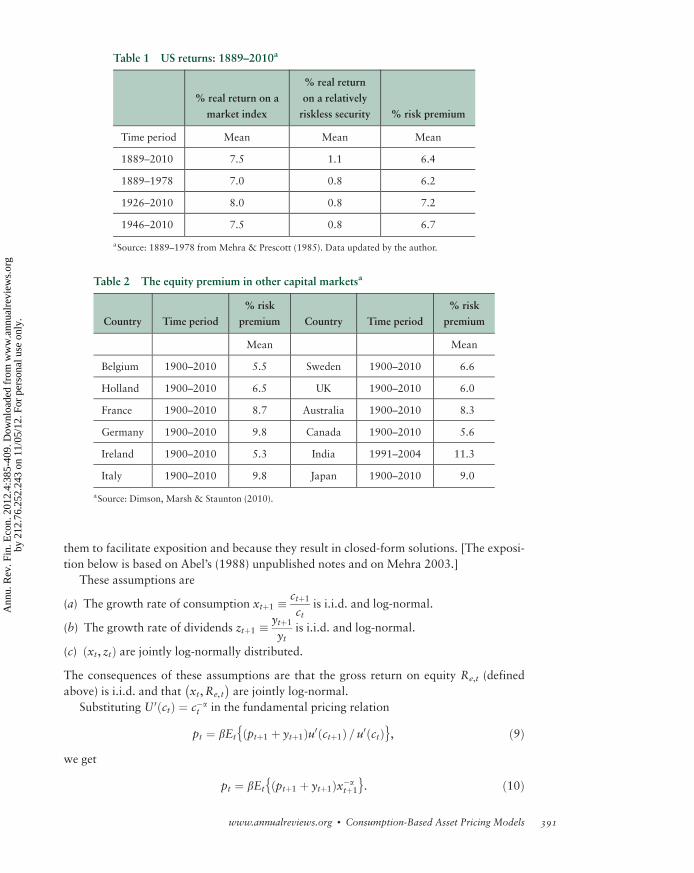
US stock returns have been considerably higher than returns for T-bills. As Table 1 shows,

the average annual real return (that is, the inflation-adjusted return) on the US stock

market for the past 120 years has been �7.5%. In the same period, the real return on a

relatively riskless security was 1.1%.

The difference between these two returns, 6.4 percentage points, is the equity premium.

Furthermore, this pattern of excess returns to equity holdings is not unique to US capital

markets. Table 2 confirms that equity returns in other developed countries also exhibit this

historical regularity when compared with the return to debt holdings. Together, the United

States, the United Kingdom, Japan, Germany, and France account for more than 85% of

capitalized global equity value.

The question that must be addressed is the following: Is the magnitude of the covari-

ance between asset returns and the marginal utility of consumption in Equation 6 large

enough to justify the observed 6% equity premium in US equity markets?

To address this issue, I make some additional assumptions. Although they are not

necessary and were not, in fact, part of the original paper on the equity premium, I include

15In contrast to our approach, which is in the applied general equilibrium tradition, there is another tradition of

testing Euler equations (such as Equation 9) and rejecting them. Hansen & Singleton (1982) and Grossman & Shiller

(1981) exemplify this approach. See Cochrane (2008) for an excellent discussion.

390 Mehra

Ann

u. R

ev. F

in. E

con.

201

2.4:

385-

409.

Dow

nloa

ded

from

ww

w.a

nnua

lrev

iew

s.or

gby

212

.76.

252.

243

on 1

1/05

/12.

For

per

sona

l use

onl

y.

them to facilitate exposition and because they result in closed-form solutions. [The exposi-

tion below is based on Abel’s (1988) unpublished notes and on Mehra 2003.]

These assumptions are

(a) The growth rate of consumption xtþ1 � ctþ1

ctis i.i.d. and log-normal.

(b) The growth rate of dividends ztþ1 � ytþ1

ytis i.i.d. and log-normal.

(c) xt, ztð Þ are jointly log-normally distributed.

The consequences of these assumptions are that the gross return on equity Re,t (defined

above) is i.i.d. and that xt,Re, t

� �are jointly log-normal.

Substituting U 0 ctð Þ ¼ c�at in the fundamental pricing relation

pt ¼ bEtf ptþ1 þ ytþ1ð Þu0 ctþ1ð Þ = u0 ctð Þg, ð9Þwe get

pt ¼ bEtf ptþ1 þ ytþ1ð Þx�atþ1g. ð10Þ

Table 1 US returns: 1889–2010a

% real return on a

market index

% real return

on a relatively

riskless security % risk premium

Time period Mean Mean Mean

1889–2010 7.5 1.1 6.4

1889–1978 7.0 0.8 6.2

1926–2010 8.0 0.8 7.2

1946–2010 7.5 0.8 6.7

aSource: 1889–1978 from Mehra & Prescott (1985). Data updated by the author.

Table 2 The equity premium in other capital marketsa

Country Time period

% risk

premium Country Time period

% risk

premium

Mean Mean

Belgium 1900–2010 5.5 Sweden 1900–2010 6.6

Holland 1900–2010 6.5 UK 1900–2010 6.0

France 1900–2010 8.7 Australia 1900–2010 8.3

Germany 1900–2010 9.8 Canada 1900–2010 5.6

Ireland 1900–2010 5.3 India 1991–2004 11.3

Italy 1900–2010 9.8 Japan 1900–2010 9.0

aSource: Dimson, Marsh & Staunton (2010).

www.annualreviews.org � Consumption-Based Asset Pricing Models 391

Ann

u. R

ev. F

in. E

con.

201

2.4:

385-

409.

Dow

nloa

ded

from

ww

w.a

nnua

lrev

iew

s.or

gby

212

.76.

252.

243

on 1

1/05

/12.

For

per

sona

l use

onl

y.

As pt is homogeneous of degree one in yt , we can represent it as

pt ¼ wyt,

and hence Re,tþ1 can be expressed as

Re,tþ1 ¼ wþ 1ð Þw

� ytþ1

yt¼ wþ 1

w� ztþ1. ð11Þ

It is easily shown that

w ¼ bEt ztþ1x�atþ1

� �1� bEt ztþ1x�a

tþ1

� � , ð12Þ

hence

Et Re,tþ1

� � ¼ Et ztþ1f gbEt ztþ1x�a

tþ1

� � . ð13Þ

Analogously, the gross return on the riskless asset can be written as

Rf , tþ1 ¼ 1

b1

Et x�atþ1

� � . ð14Þ

Given that I have assumed the growth rate of consumption and dividends to be log-normally

distributed, the unconditional expectation of Equation 13 is

EfReg ¼ emzþ1=2s2z

bemz�amxþ1=2 s2zþa2s2x�2asx, zð Þ , ð15Þ

and

lnEfReg ¼ �ln bþ amx � 1 =2a2s2x þ asx,z, ð16Þwhere mx ¼ Eðln xÞ, s2x ¼ Varðln xÞ, sx,z ¼ Covðln x, ln zÞ, and ln x is the continuously

compounded growth rate of consumption. The other terms involving z and Re are

defined analogously.

Similarly,

Rf ¼1

be�amxþ1=2a2s2x, ð17Þ

and

ln Rf ¼ �ln bþ amx � 1 = 2a2s2x ð18Þ

ln EfReg � ln Rf ¼ asx, z. ð19ÞFrom Equation 11 it also follows that

ln EfReg � ln Rf ¼ asx,Re, ð20Þ

where sx,Re¼ Cov ln x, ln Reð Þ.

The (log) equity premium in this model is the product of the coefficient of relative risk

aversion and the covariance of the (continuously compounded) growth rate of consumption

392 Mehra

Ann

u. R

ev. F

in. E

con.

201

2.4:

385-

409.

Dow

nloa

ded

from

ww

w.a

nnua

lrev

iew

s.or

gby

212

.76.

252.

243

on 1

1/05

/12.

For

per

sona

l use

onl

y.

with the (continuously compounded) return on equity or the growth rate of dividends. If we

impose the equilibrium condition that x ¼ z, a consequence of which is the restriction that

the return on equity is perfectly correlated to the growth rate of consumption, we get

lnEfReg � lnRf ¼ as2x, ð21Þand the equity premium then is the product of the coefficient of relative risk aversion and

the variance of the growth rate of consumption.

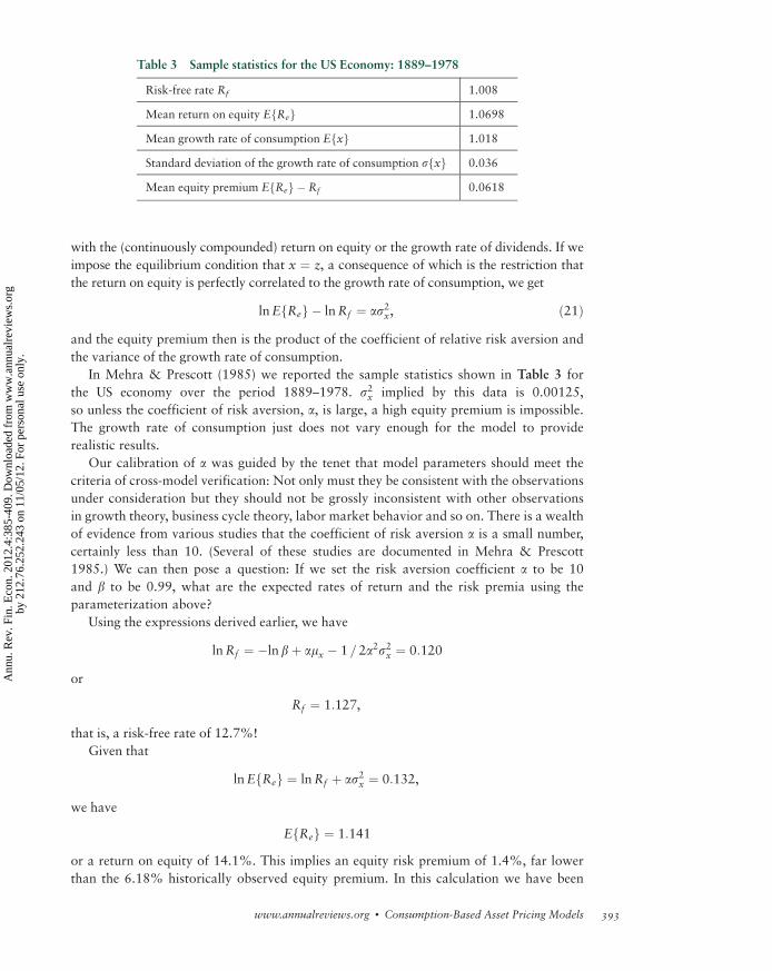
In Mehra & Prescott (1985) we reported the sample statistics shown in Table 3 for

the US economy over the period 1889–1978. s2x implied by this data is 0.00125,

so unless the coefficient of risk aversion, a, is large, a high equity premium is impossible.

The growth rate of consumption just does not vary enough for the model to provide

realistic results.

Our calibration of a was guided by the tenet that model parameters should meet the

criteria of cross-model verification: Not only must they be consistent with the observations

under consideration but they should not be grossly inconsistent with other observations

in growth theory, business cycle theory, labor market behavior and so on. There is a wealth

of evidence from various studies that the coefficient of risk aversion a is a small number,

certainly less than 10. (Several of these studies are documented in Mehra & Prescott

1985.) We can then pose a question: If we set the risk aversion coefficient a to be 10

and b to be 0.99, what are the expected rates of return and the risk premia using the

parameterization above?

Using the expressions derived earlier, we have

lnRf ¼ �ln bþ amx � 1 =2a2s2x ¼ 0:120

or

Rf ¼ 1:127,

that is, a risk-free rate of 12.7%!

Given that

lnEfReg ¼ lnRf þ as2x ¼ 0:132,

we have

EfReg ¼ 1:141

or a return on equity of 14.1%. This implies an equity risk premium of 1.4%, far lower

than the 6.18% historically observed equity premium. In this calculation we have been

Table 3 Sample statistics for the US Economy: 1889–1978

Risk-free rate Rf 1.008

Mean return on equity E Ref g 1.0698

Mean growth rate of consumption E xf g 1.018

Standard deviation of the growth rate of consumption s xf g 0.036

Mean equity premium E Ref g � Rf 0.0618

www.annualreviews.org � Consumption-Based Asset Pricing Models 393

Ann

u. R

ev. F

in. E

con.

201

2.4:

385-

409.

Dow

nloa

ded

from

ww

w.a

nnua

lrev

iew

s.or

gby

212

.76.

252.

243

on 1

1/05

/12.

For

per

sona

l use

onl

y.

liberal in choosing values for a and b. Most studies indicate a value for a that is close to 3.

If we pick a lower value for b, the risk-free rate will be even higher and the premium

lower. Accordingly, the 1.4% value represents the maximum equity risk premium that

can be obtained in this class of models given the constraints on a and b. Given that the

observed equity premium is more than 6%, it is puzzling that risk considerations alone

cannot account for the equity premium within the complete markets, representative house-

hold construct.

3.1. The Risk-Free Rate Puzzle

Philippe Weil (1989) has dubbed the high risk-free rate obtained above the risk-free rate

puzzle. The short-term real rate in the United States averages less than 1%, while the high

value of a required to generate the observed equity premium results in an unacceptably

high risk-free rate. The risk-free rate as shown in Equation 18 can be decomposed into

three components:

lnRf ¼ �ln bþ amx � 1 = 2a2s2x.

The first term, �ln b, is a time preference or impatience term. When b < 1 it reflects the

fact that agents prefer early consumption to later consumption. Thus, in a world of perfect

certainty and no growth in consumption, the unique interest rate in the economy will

be Rf ¼ 1 =b.The second term, amx, arises because of growth in consumption. If consumption is

likely to be higher in the future, agents with concave utility will prefer to borrow against

future consumption to smooth their lifetime consumption. The greater the curvature of

the utility function and the larger the growth rate of consumption, the greater the desire

to smooth consumption. In equilibrium, this will lead to a higher interest rate given that

agents in the aggregate cannot simultaneously increase their current consumption.

The third term, 1 = 2a2s2x, arises from a demand for precautionary savings. In a world

of uncertainty, agents like to hedge against future unfavorable consumption realizations

by building buffer stocks of the consumption good. Hence, in equilibrium the interest

rate must fall to counter this enhanced demand for savings.

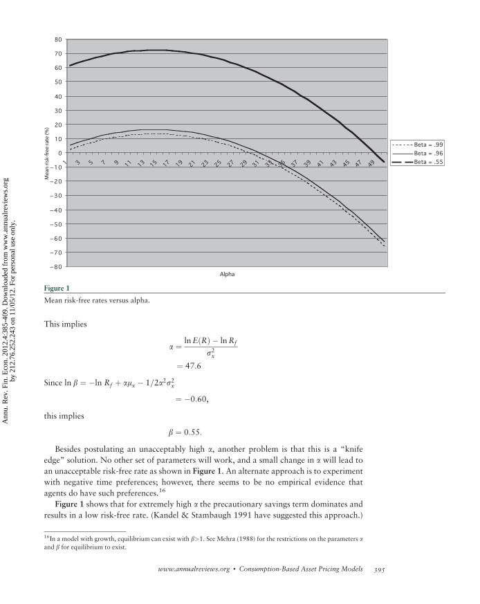
Figure 1 plots lnRf ¼ �ln bþ amx � 1 = 2a2s2x calibrated to the US historical values,

with mx ¼ 0:0172 and s2x ¼ 0:00125 for various values of b. It shows that the precau-

tionary savings effect is negligible for reasonable values of a 1<a<5ð Þ.For a ¼ 3 and b ¼ 0.99, Rf ¼ 1.058, which implies a risk-free rate of 5.8%—much

higher than the historical mean rate of 0.8%. The economic intuition is straightforward:

With consumption growing at 1.8% a year with a standard deviation of 3.6%, agents

with isoelastic preferences have a sufficiently strong desire to borrow to smooth con-

sumption that it takes a high interest rate to induce them not to do so.

The late Fischer Black (private communication) proposed that a ¼ 55 would solve the

puzzle. Indeed the 1889–1978 US experience reported above can be reconciled with

a ¼ 48 and b ¼ 0.55.

To see this, observe that since s2x ¼ ln 1þ var xð ÞE xð Þ½ �2

" #¼ 0:00125

and

mx ¼ ln E xð Þ � 1=2s2x ¼ 0:0172:

394 Mehra

Ann

u. R

ev. F

in. E

con.

201

2.4:

385-

409.

Dow

nloa

ded

from

ww

w.a

nnua

lrev

iew

s.or

gby

212

.76.

252.

243

on 1

1/05

/12.

For

per

sona

l use

onl

y.

This implies

a ¼ lnE Rð Þ � lnRf

s2x¼ 47:6

Since ln b ¼ �ln Rf þ amx � 1=2a2s2x

¼ �0:60,

this implies

b ¼ 0:55:

Besides postulating an unacceptably high a, another problem is that this is a “knife

edge” solution. No other set of parameters will work, and a small change in a will lead to

an unacceptable risk-free rate as shown in Figure 1. An alternate approach is to experiment

with negative time preferences; however, there seems to be no empirical evidence that

agents do have such preferences.16

Figure 1 shows that for extremely high a the precautionary savings term dominates and

results in a low risk-free rate. (Kandel & Stambaugh 1991 have suggested this approach.)

16In a model with growth, equilibrium can exist with b>1. See Mehra (1988) for the restrictions on the parameters aand b for equilibrium to exist.

Figure 1

Mean risk-free rates versus alpha.

www.annualreviews.org � Consumption-Based Asset Pricing Models 395

Ann

u. R

ev. F

in. E

con.

201

2.4:

385-

409.

Dow

nloa

ded

from

ww

w.a

nnua

lrev

iew

s.or

gby

212

.76.

252.

243

on 1

1/05

/12.

For

per

sona

l use

onl

y.

However, then a small change in the growth rate of consumption will have a large impact

on interest rates. This is inconsistent with a cross-country comparison of real risk-free rates

and their observed variability. For example, throughout the 1980s, South Korea had a

much higher growth rate than the United States but real rates were not appreciably higher.

Nor does the risk-free rate vary considerably over time, as would be expected if a was

large. In Section 4 I show how alternative preference structures can help resolve the risk-

free rate puzzle.

3.2. Hansen-Jagannathan Bounds

An alternative perspective on the puzzle is provided by Hansen & Jagannathan (1991).

The fundamental pricing equation can be written as

Et Re,tþ1

� � ¼ Rf ,tþ1 þ Covtmtþ1,t,Re,tþ1

Et mtþ1,t

� �( )

. ð22Þ

This expression also holds unconditionally so that

E Re,tþ1

� � ¼ Rf ,tþ1 þ s mtþ1,t

� �s Re,tþ1

� �rRe,m =Et mtþ1, t

� � ð23Þ

or

E Re,tþ1

� �� Rf ,tþ1 = s Re,tþ1

� � ¼ s mtþ1,t

� �rRe,m =Et mtþ1,t

� �� ð24Þ

and given that

�1 � rRe,m� 1,

j E Re,tþ1

� �� Rf ,tþ1

� �= s Re,tþ1

� �j � s mtþ1,t

� �=E mtþ1,t

� �. ð25Þ

This inequality is referred to as the Hansen-Jagannathan lower bound on the pricing kernel.

For the US economy, the Sharpe Ratio, E Re,tþ1

� �� Rf ,tþ1

� �= s Re,tþ1

� �, can be calcu-

lated to be 0.37. Given that E mtþ1,t

� �is the expected price of a one-period risk-free

bond, its value must be close to 1. In fact, for the parameterization discussed earlier,

E mtþ1,t

� � ¼ 0:96 when a ¼ 2. This implies that the lower bound on the standard deviation

for the pricing kernel must be close to 0.3 if the Hansen-Jagannathan bound is to be

satisfied. However, when this is calculated in the Mehra-Prescott framework, we obtain

an estimate for s mtþ1,t

� � ¼ 0:002, which is off by more than an order of magnitude.

I would like to emphasize that the equity premium puzzle is a quantitative puzzle;

standard theory is consistent with our notion of risk that, on average, stocks should return

more than bonds. The puzzle arises because quantitative predictions of the theory are an

order of magnitude different from what has been historically documented. The puzzle

cannot be dismissed lightly, given that much of our economic intuition is based on the very

class of models that fall short so dramatically when confronted with financial data.

It underscores the failure of paradigms central to financial and economic modeling to

capture the characteristic that appears to make stocks comparatively so risky. Hence the

viability of using this class of models for any quantitative assessment, say, to gauge the

welfare implications of alternative stabilization policies, is thrown open to question.

For this reason, over the past 20 years or so, attempts to resolve the puzzle have become

a major research impetus in both finance and economics. Several generalizations of key

396 Mehra

Ann

u. R

ev. F

in. E

con.

201

2.4:

385-

409.

Dow

nloa

ded

from

ww

w.a

nnua

lrev

iew

s.or

gby

212

.76.

252.

243

on 1

1/05

/12.

For

per

sona

l use

onl

y.

features of the Mehra & Prescott (1985) model have been proposed to better reconcile

observations with theory. These include alternative assumptions on preferences,17 modi-

fied probability distributions to admit rare but disastrous events,18 survival bias,19 incomplete

markets,20 and market imperfections.21 They also include attempts at modeling limited

participation of consumers in the stock market (Attanasio, Banks & Tanner 2002; Brav,

Constantinides & Geczy 2002; Mankiw & Zeldes 1991; and Vissing-Jorgensen 2002), and

problems of temporal aggregation (Gabaix & Laibson 2001, Heaton 1995, and Lynch 1996).

The reader is referred to the essays in the Handbook of the Equity Risk Premium (Mehra

2008) for a comprehensive review of this vast literature. (Other excellent surveys include

Kocherlakota 1996, Campbell 2001, and Ludvigson 2012.) I briefly summarize some of the

research efforts to resolve the puzzle in Sections 4 and 5 below. Section 4 explores explana-

tions of the equity premium puzzle based on alternative preference specifications. Section 5, in

contrast, reviews the nascent literature that takes as given the findings in Mehra & Prescott

(1985) and tries to account for the equity premium by factors other than aggregate risk.

4. ALTERNATIVE PREFERENCE ORDERINGS

The analysis above shows that the CRRA preferences used inMehra& Prescott (1985) can only

bemade consistent with the observed equity premium if the coefficient of relative risk aversion is

implausibly large. In an effort to reconcile theory with observations, in this section I explore

stochastic discount factor processes, fms,tg, implied by preferences other than CRRA.

There is an extensive literature22 that explores preferences other than CRRA, defined

over per capita consumption sequences. A major drawback of these alternative preference

structures is that none of them permits aggregation and some are time inconsistent.23 In the

discussion below, I discuss in detail the most widely used alternate preference classes,

Generalized Expected Utility (GEU) and Habit Formation.

Although these preferences do not permit aggregation, they are time consistent.

4.1. Generalized Expected Utility

One restriction imposed by the CRRA class of preferences is that the coefficient of risk

aversion is rigidly linked to the elasticity of intertemporal substitution; one is the reciprocal

17For example, see Abel (1990); Bansal & Yaron (2004); Benartzi & Thaler (1995); Boldrin, Christiano & Fisher

(2001); Campbell & Cochrane (1999); Constantinides (1990); Epstein & Zin (1991); Ferson & Constantinides

(1991); and Hansen, Heaton & Li (2008).

18See Barro (2006), Barro & Ursua (2008), Constantinides (2008), Donaldson & Mehra (2008), Rietz (1988), and

Mehra & Prescott (1988).

19Brown, Goetzmann & Ross (1995).

20For example, Bewley (1982); Brav, Constantinides & Geczy (2002); Constantinides & Duffie (1996); Heaton &

Lucas (1997, 2000); Lucas (1994); Mankiw (1986); Mehra & Prescott (1985); Storesletten, Telmer & Yaron (2007);

and Telmer (1993).

21For example, Aiyagari & Gertler (1991); Alvarez & Jermann (2000); Bansal & Coleman (1996); Basak & Cuoco

(1998); Constantinides, Donaldson & Mehra (2002); Danthine, Donaldson & Mehra (1992); Daniel & Marshall

(1997); He & Modest (1995); Heaton & Lucas (1996); Luttmer (1996); McGrattan & Prescott (2001); and

Storesletten, Telmer & Yaron (2004).

22I refer the reader to Donaldson & Mehra (2008) for a detailed review.

23See the discussion in Section 2 on the desirability of these characteristics.

www.annualreviews.org � Consumption-Based Asset Pricing Models 397

Ann

u. R

ev. F

in. E

con.

201

2.4:

385-

409.

Dow

nloa

ded

from

ww

w.a

nnua

lrev

iew

s.or

gby

212

.76.

252.

243

on 1

1/05

/12.

For

per

sona

l use

onl

y.

of the other. What this implies is that if an individual is averse to variation of consump-

tion across different states at a particular point of time then he will be averse to con-

sumption variation over time. There is no a priori reason that this must be. Given that, on

average, consumption is growing over time, the agents in the Mehra & Prescott (1985)

setup have little incentive to save. The demand for bonds is low and as a consequence,

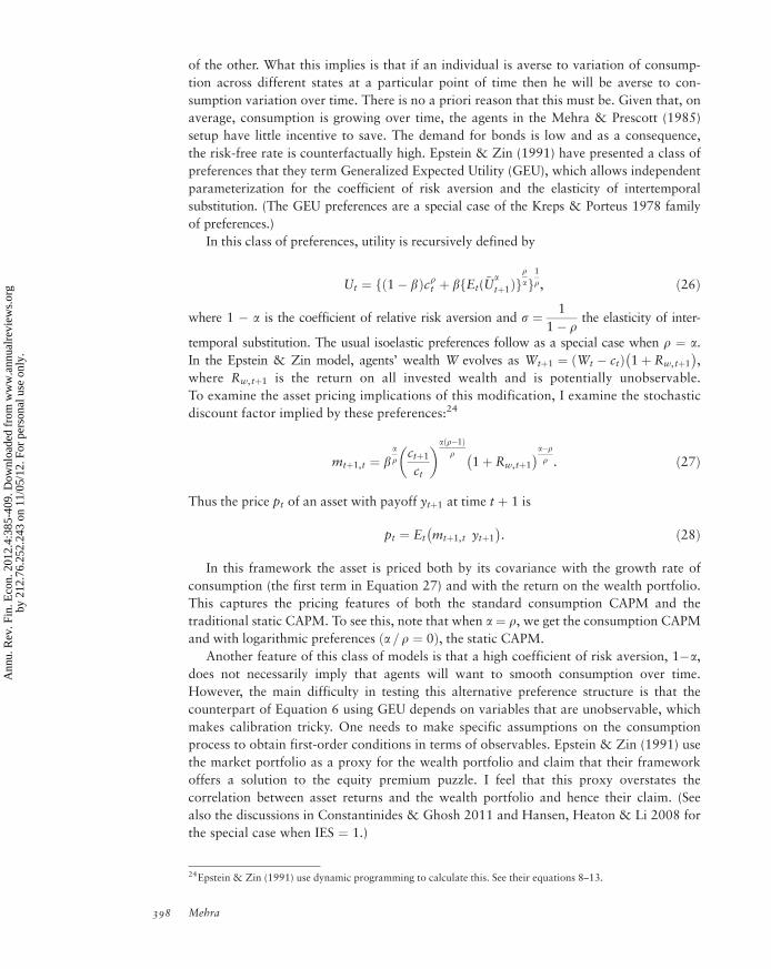
the risk-free rate is counterfactually high. Epstein & Zin (1991) have presented a class of

preferences that they term Generalized Expected Utility (GEU), which allows independent

parameterization for the coefficient of risk aversion and the elasticity of intertemporal

substitution. (The GEU preferences are a special case of the Kreps & Porteus 1978 family

of preferences.)

In this class of preferences, utility is recursively defined by

Ut ¼ f 1� bð Þcrt þ bfEt(~Uatþ1Þg

rag

1

r, ð26Þ

where 1 � a is the coefficient of relative risk aversion and s ¼ 1

1� rthe elasticity of inter-

temporal substitution. The usual isoelastic preferences follow as a special case when r ¼ a.In the Epstein & Zin model, agents’ wealth W evolves as Wtþ1 ¼ Wt � ctð Þ 1þ Rw, tþ1

� �,

where Rw, tþ1 is the return on all invested wealth and is potentially unobservable.

To examine the asset pricing implications of this modification, I examine the stochastic

discount factor implied by these preferences:24

mtþ1,t ¼ bar

ctþ1

ct

� a r�1ð Þr

1þ Rw,tþ1

� �a�rr . ð27Þ

Thus the price pt of an asset with payoff ytþ1 at time t þ 1 is

pt ¼ Et mtþ1,t ytþ1

� �. ð28Þ

In this framework the asset is priced both by its covariance with the growth rate of

consumption (the first term in Equation 27) and with the return on the wealth portfolio.

This captures the pricing features of both the standard consumption CAPM and the

traditional static CAPM. To see this, note that when a ¼ r, we get the consumption CAPM

and with logarithmic preferences a =r ¼ 0ð Þ, the static CAPM.

Another feature of this class of models is that a high coefficient of risk aversion, 1�a,does not necessarily imply that agents will want to smooth consumption over time.

However, the main difficulty in testing this alternative preference structure is that the

counterpart of Equation 6 using GEU depends on variables that are unobservable, which

makes calibration tricky. One needs to make specific assumptions on the consumption

process to obtain first-order conditions in terms of observables. Epstein & Zin (1991) use

the market portfolio as a proxy for the wealth portfolio and claim that their framework

offers a solution to the equity premium puzzle. I feel that this proxy overstates the

correlation between asset returns and the wealth portfolio and hence their claim. (See

also the discussions in Constantinides & Ghosh 2011 and Hansen, Heaton & Li 2008 for

the special case when IES ¼ 1.)

24Epstein & Zin (1991) use dynamic programming to calculate this. See their equations 8–13.

398 Mehra

Ann

u. R

ev. F

in. E

con.

201

2.4:

385-

409.

Dow

nloa

ded

from

ww

w.a

nnua

lrev

iew

s.or

gby

212

.76.

252.

243

on 1

1/05

/12.

For

per

sona

l use

onl

y.

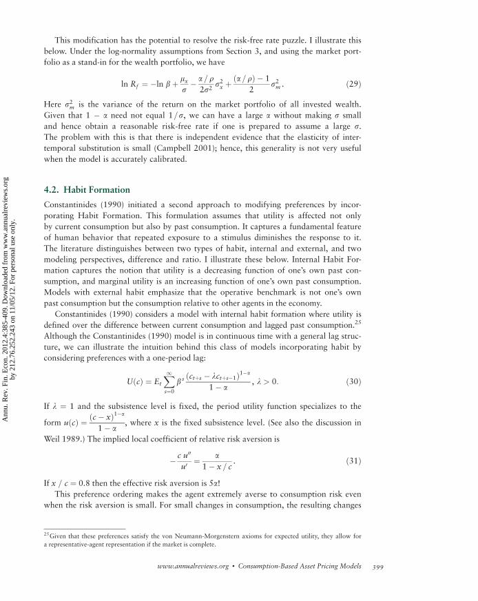
This modification has the potential to resolve the risk-free rate puzzle. I illustrate this

below. Under the log-normality assumptions from Section 3, and using the market port-

folio as a stand-in for the wealth portfolio, we have

ln Rf ¼ �ln bþ mxs� a =r

2s2s2x þ

a = rð Þ � 1

2s2m . ð29Þ

Here s2m is the variance of the return on the market portfolio of all invested wealth.

Given that 1 � a need not equal 1=s, we can have a large a without making s small

and hence obtain a reasonable risk-free rate if one is prepared to assume a large s.The problem with this is that there is independent evidence that the elasticity of inter-

temporal substitution is small (Campbell 2001); hence, this generality is not very useful

when the model is accurately calibrated.

4.2. Habit Formation

Constantinides (1990) initiated a second approach to modifying preferences by incor-

porating Habit Formation. This formulation assumes that utility is affected not only

by current consumption but also by past consumption. It captures a fundamental feature

of human behavior that repeated exposure to a stimulus diminishes the response to it.

The literature distinguishes between two types of habit, internal and external, and two

modeling perspectives, difference and ratio. I illustrate these below. Internal Habit For-

mation captures the notion that utility is a decreasing function of one’s own past con-

sumption, and marginal utility is an increasing function of one’s own past consumption.

Models with external habit emphasize that the operative benchmark is not one’s own

past consumption but the consumption relative to other agents in the economy.

Constantinides (1990) considers a model with internal habit formation where utility is

defined over the difference between current consumption and lagged past consumption.25

Although the Constantinides (1990) model is in continuous time with a general lag struc-

ture, we can illustrate the intuition behind this class of models incorporating habit by

considering preferences with a one-period lag:

U cð Þ ¼ Et

X1s¼0

b s ctþs � lctþs�1ð Þ1�a

1� a, l > 0: ð30Þ

If l ¼ 1 and the subsistence level is fixed, the period utility function specializes to the

form u cð Þ ¼ c� xð Þ1�a

1� a, where x is the fixed subsistence level. (See also the discussion in

Weil 1989.) The implied local coefficient of relative risk aversion is

� c u00

u0¼ a

1� x = c. ð31Þ

If x = c ¼ 0.8 then the effective risk aversion is 5a!This preference ordering makes the agent extremely averse to consumption risk even

when the risk aversion is small. For small changes in consumption, the resulting changes

25Given that these preferences satisfy the von Neumann-Morgenstern axioms for expected utility, they allow for

a representative-agent representation if the market is complete.

www.annualreviews.org � Consumption-Based Asset Pricing Models 399

Ann

u. R

ev. F

in. E

con.

201

2.4:

385-

409.

Dow

nloa

ded

from

ww

w.a

nnua

lrev

iew

s.or

gby

212

.76.

252.

243

on 1

1/05

/12.

For

per

sona

l use

onl

y.

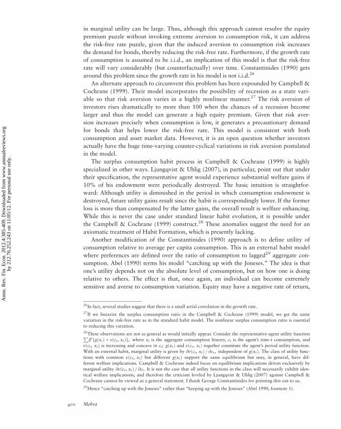
in marginal utility can be large. Thus, although this approach cannot resolve the equity

premium puzzle without invoking extreme aversion to consumption risk, it can address

the risk-free rate puzzle, given that the induced aversion to consumption risk increases

the demand for bonds, thereby reducing the risk-free rate. Furthermore, if the growth rate

of consumption is assumed to be i.i.d., an implication of this model is that the risk-free

rate will vary considerably (but counterfactually) over time. Constantinides (1990) gets

around this problem since the growth rate in his model is not i.i.d.26

An alternate approach to circumvent this problem has been expounded by Campbell &

Cochrane (1999). Their model incorporates the possibility of recession as a state vari-

able so that risk aversion varies in a highly nonlinear manner.27 The risk aversion of

investors rises dramatically to more than 100 when the chances of a recession become

larger and thus the model can generate a high equity premium. Given that risk aver-

sion increases precisely when consumption is low, it generates a precautionary demand

for bonds that helps lower the risk-free rate. This model is consistent with both

consumption and asset market data. However, it is an open question whether investors

actually have the huge time-varying counter-cyclical variations in risk aversion postulated

in the model.

The surplus consumption habit process in Campbell & Cochrane (1999) is highly

specialized in other ways. Ljungqvist & Uhlig (2007), in particular, point out that under

their specification, the representative agent would experience substantial welfare gains if

10% of his endowment were periodically destroyed. The basic intuition is straightfor-

ward: Although utility is diminished in the period in which consumption endowment is

destroyed, future utility gains result since the habit is correspondingly lower. If the former

loss is more than compensated by the latter gains, the overall result is welfare enhancing.

While this is never the case under standard linear habit evolution, it is possible under

the Campbell & Cochrane (1999) construct.28 These anomalies suggest the need for an

axiomatic treatment of Habit Formation, which is presently lacking.

Another modification of the Constantinides (1990) approach is to define utility of

consumption relative to average per capita consumption. This is an external habit model

where preferences are defined over the ratio of consumption to lagged29 aggregate con-

sumption. Abel (1990) terms his model “catching up with the Joneses.” The idea is that

one’s utility depends not on the absolute level of consumption, but on how one is doing

relative to others. The effect is that, once again, an individual can become extremely

sensitive and averse to consumption variation. Equity may have a negative rate of return,

26In fact, several studies suggest that there is a small serial correlation in the growth rate.

27If we linearize the surplus consumption ratio in the Campbell & Cochrane (1999) model, we get the same

variation in the risk-free rate as in the standard habit model. The nonlinear surplus consumption ratio is essential

to reducing this variation.

28These observations are not as general as would initially appear. Consider the representative-agent utility functionPbt g xtð Þ þ v ct, xtð Þf g, where xt is the aggregate consumption history, ct is the agent’s time-t consumption, and

v ct, xtð Þ is increasing and concave in ct; g xtð Þ and v ct, xtð Þ together constitute the agent’s period utility function.

With an external habit, marginal utility is given by @v ct , xtð Þ = @ct, independent of g xtð Þ. The class of utility func-

tions with common v ct, xtð Þ but different g xtð Þ support the same equilibrium but may, in general, have dif-

ferent welfare implications. Campbell & Cochrane indeed focus on equilibrium implications driven exclusively by

marginal utility @v ct, xtð Þ = @ct. It is not the case that all utility functions in the class will necessarily exhibit iden-

tical welfare implications, and therefore the criticism leveled by Ljungqvist & Uhlig (2007) against Campbell &

Cochrane cannot be viewed as a general statement. I thank George Constantinides for pointing this out to us.

29Hence “catching up with the Joneses” rather than “keeping up with the Joneses” (Abel 1990, footnote 1).

400 Mehra

Ann

u. R

ev. F

in. E

con.

201

2.4:

385-

409.

Dow

nloa

ded

from

ww

w.a

nnua

lrev

iew

s.or

gby

212

.76.

252.

243

on 1

1/05

/12.

For

per

sona

l use

onl

y.

and this can result in personal consumption falling relative to others. Equity thus becomes

an undesirable asset relative to bonds. Given that average per capita consumption is rising

over time, the induced demand for bonds with this modification helps to mitigate the

risk-free rate puzzle.

Abel (1990) defines utility as the ratio of consumption relative to average per capita

consumption rather than the difference between the two. This is not a trivial modification

(see Campbell 2001 for a detailed discussion). While difference habit models can, in

principle, generate a high equity premium, ratio models generate a premium that is similar

to that obtained with standard preferences.

To summarize, models with Habit Formation and relative or subsistence consumption

have had success in addressing the risk-free rate puzzle but only limited success in resolving

the equity premium puzzle, since in these models effective risk aversion and prudence

become implausibly large.

5. NON-RISK-BASED EXPLANATIONS OF THE EQUITY PREMIUM

In this section I review the literature that takes as given the findings in Mehra & Prescott

(1985) and tries to account for the equity premium by factors other than aggregate risk.

Much of this literature reexamines the appropriateness of the abstractions and assump-

tions made in our original paper. In particular, the appropriateness of using T-bills as a

proxy for the intertemporal marginal rate of substitution of consumption, ignoring the

difference between borrowing and lending rates (a consequence of agent heterogeneity and

costly intermediation), abstracting from life-cycle effects and borrowing constraints on the

young, and the abstraction from regulations and taxes. I consider each in turn and examine

the impact on the equity premium.

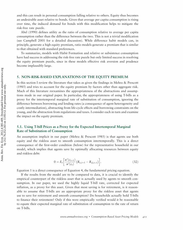
5.1. Using T-bill Prices as a Proxy for the Expected Intertemporal MarginalRate of Substitution of Consumption

An assumption implicit in our paper (Mehra & Prescott 1985) is that agents use both

equity and the riskless asset to smooth consumption intertemporally. This is a direct

consequence of the first-order condition (below) for the representative household in our

model, which implies that agents save by optimally allocating resources between equity

and riskless debt:

0 ¼ Etu 0 ctþ1ð Þu 0 ctð Þ Re,tþ1 � Rd,tþ1

� � �. ð32Þ

Equation 1 is a direct consequence of Equation 4, the fundamental pricing equation.

If the results from the model are to be compared to data, it is crucial to identify the

empirical counterpart of the riskless asset that is actually used by agents to smooth con-

sumption. In our paper, we used the highly liquid T-bill rate, corrected for expected

inflation, as a proxy for this asset. Given that most saving is for retirement, is it reason-

able to assume that T-bills are an appropriate proxy for the riskless asset that agents

use to save for retirement and smooth consumption? Do households actually hold T-bills

to finance their retirement? Only if this were empirically verified would it be reasonable

to equate their expected marginal rate of substitution of consumption to the rate of return

on T-bills.

www.annualreviews.org � Consumption-Based Asset Pricing Models 401

Ann

u. R

ev. F

in. E

con.

201

2.4:

385-

409.

Dow

nloa

ded

from

ww

w.a

nnua

lrev

iew

s.or

gby

212

.76.

252.

243

on 1

1/05

/12.

For

per

sona

l use

onl

y.

This question cannot be answered in the abstract, without reference to the asset hold-

ings of households. A natural next step then is to examine the assets held by households.

Table 4 details these holdings for American households. The four big asset-holding

categories of households are tangible assets, pension and life insurance holdings, equity

(both corporate and noncorporate), and debt assets.

In 2000, privately held government debt was valued at only 0.30 GDP, a third of

which was held by foreigners. The amount of interest-bearing government debt with

maturity less than a year was only 0.085 GDP, which is a small fraction of total house-

hold net worth. Virtually no T-bills are directly owned by households (see Counc. Econ.

Advis. 2005, table B-89 ). Approximately one-third of the T-bills outstanding are held by

foreign central banks and two-thirds by American financial institutions.

Although there are large amounts of debt assets held, most of these are in the form of

pension fund and life insurance reserves. Some are in the form of demand deposits, for

which free services are provided. Most of the government debt is held indirectly; a small

fraction is held as savings bonds that people give to their grandchildren.

Thus, much of intertemporal saving is in debt assets such as annuities and mortgage

debt held in retirement accounts and as pension fund reserves. Other assets, not T-bills,

are typically held to finance consumption when old. Hence, T-bills and short-term debt

are not reasonable empirical counterparts to the risk-free asset being priced in Equation 1,

and it would be inappropriate to equate the return on these assets to the expected marginal

rate of substitution for an important group of agents.

An inflation-indexed, default-free bond portfolio with a duration similar to that of a

well-diversified equity portfolio would be a reasonable proxy for a risk-free asset used

for consumption smoothing. (McGrattan & Prescott 2003 use long-term, high-grade

municipal bonds as a proxy for the riskless security.) For most of the twentieth century,

equity has had an implied duration of �25 years, so a portfolio of TIPS of a similar

duration would be a reasonable proxy.

Since TIPS have only recently (1997) been introduced in US capital markets, it is

difficult to get accurate estimates of the mean return on this asset class. The average return

for the 1997–2005 period is 3.7%. An alternative (though imperfect) proxy would be to

use the returns on indexed mortgages guaranteed by Ginnie Mae or issued by Fannie Mae.

I conjecture that if these indexed default-free securities are used as a benchmark, the

equity premium would be closer to 4% than to the 6% equity premium relative to T-bills.

By using the more appropriate benchmark for the riskless asset, we would have accounted

for two percentage points of the equity premium.

Table 4 Household assets and liabilities as a fraction/multiple of GDP (average of 2000

and 2005)

Assets (GDP) Liabilities (GDP)

Tangible household

Corporate equity

Noncorporate equity

Pension and life insurance reserves

Debt assets

1.65

0.85

0.5

1.0

0.85

Liabilities

Net worth

0.7

4.15

Total 4.85 Total 4.85

402 Mehra

Ann

u. R

ev. F

in. E

con.

201

2.4:

385-

409.

Dow

nloa

ded

from

ww

w.a

nnua

lrev

iew

s.or

gby

212

.76.

252.

243

on 1

1/05

/12.

For

per

sona

l use

onl

y.

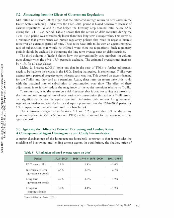
5.2. Abstracting from the Effects of Government Regulations

McGrattan & Prescott (2003) argue that the estimated average return on debt assets in the

United States (including T-bills) over the 1926–2000 period is biased downward because of

various regulations (W and X) that helped the Treasury keep nominal rates below 2.5%

during the 1941–1954 period. Table 5 shows that the return on debt securities during the

1941–1954 period was considerably lower than their long-term average value. This serves as

a reminder that governments can pursue regulatory policies that result in negative interest

rates over an extended period of time. These rates have little to do with an agent’s marginal

rate of substitution that would be inferred were there no regulations. Such regulatory

periods should be excluded in estimating the long-term average rates on debt securities.

The third column in Table 5 shows how the conventionally used numbers (in column

two) change when the 1941–1954 period is excluded. The estimated average rates increase

by �1% for all asset classes.

Mehra & Prescott (2008b) point out that in the case of T-bills a further adjustment

needs to be made to the returns in the 1930s. During that period, in some states, T-bills were

exempt from personal property taxes whereas cash was not. This created an excess demand

for the T-bills, and they sold at a premium. Again, these rates on return have little to do

with the marginal rate of substitution of consumption over time. The effect of these

adjustments is to further reduce the magnitude of the equity premium relative to T-bills.

To summarize, using the return on a risk-free asset that is used for saving as a proxy for

the intertemporal marginal rate of substitution of consumption (instead of a T-bill return)

can significantly reduce the equity premium. Adjusting debt returns for government

regulations further reduces the historical equity premium over the 1926–2000 period by

1% irrespective of the debt asset used as a benchmark.

The adjustments suggested in Sections 5.1 and 5.2 suggest that 3% of the equity

premium reported in Mehra & Prescott (1985) can be accounted for by factors other than

aggregate risk.

5.3. Ignoring the Difference Between Borrowing and Lending Rates:A Consequence of Agent Heterogeneity and Costly Intermediation

A major disadvantage of the homogeneous household construct is that it precludes the

modeling of borrowing and lending among agents. In equilibrium, the shadow price of

Table 5 US inflation-adjusted average return on debta

Period 1926–2000 1926–1940 1 1955–2000 1941–1954

US Treasury bills 0.8% 1.8% �3.6%

Intermediate-term

government bonds

2.4% 3.6% �2.7%

Long-term

government bonds

2.7% 3.8% �1.9%

Long-term

corporate bonds

3.0% 4.1% �1.9%

aSource: Ibbotson Assoc. (2001)

www.annualreviews.org � Consumption-Based Asset Pricing Models 403

Ann

u. R

ev. F

in. E

con.

201

2.4:

385-

409.

Dow

nloa

ded

from

ww

w.a

nnua

lrev

iew

s.or

gby

212

.76.

252.

243

on 1

1/05

/12.

For

per

sona

l use

onl

y.

consumption at date t þ 1 in terms of consumption at date t is such that the amount of

borrowing and lending is zero. However, there is a large amount of costly intermediated

borrowing and lending between households and, as a consequence, borrowing rates exceed

lending rates. When borrowing and lending rates differ, the following question arises:

Should the equity premium be measured relative to the riskless borrowing rate or the

riskless lending rate?

To address this, we (Mehra, Piguillem & Prescott 2011) construct a model that incor-

porates agent heterogeneity and costly financial intermediation. The resources used in

intermediation (3.4% of GNP) and the amount intermediated (1.7 GNP) imply that the

average household borrowing rate is at least 2% higher than the average household lend-

ing rate. Relative to the level of the observed average rates of return on debt and equity

securities, this spread is far from being insignificant and cannot be ignored when

addressing the equity premium.

In our model,30 a subset of households both borrows and holds equity. As a conse-

quence, a no-arbitrage condition is that the return on equity and the borrowing rate are

equal (5%). The return on government debt, the household lending rate, is 3%. If we use

the conventional definition of the equity premium—the return on a broad equity index less

the return on government debt—we would erroneously conclude that in our model the

equity premium was 2%. The difference in the government borrowing rate and the return

on equity is not an equity premium; it arises because of the wedge between borrowing

and lending rates. Analogously, if borrowing and lending rates for equity investors

differ, and they do in the US economy, the equity premium should be measured relative

to the investor borrowing rate rather than the investor lending rate (the government’s

borrowing rate). Measuring the premium relative to the government’s borrowing rate

artificially increases the premium for bearing aggregate risk by the difference between

the investor’s borrowing and lending rates. (For a detailed exposition of this and related

issues, the reader is referred to Mehra & Prescott 2008a.) If such a correction were

made and the equity premium was measured relative to the investor’s borrowing rate, it

would be further reduced by two percentage points.

5.4. Abstracting from Life-Cycle Effects and Borrowing Constraintson the Young

In Constantinides, Donaldson & Mehra (2002) we examine the impact of life-cycle

effects such as variable labor income and borrowing constraints on the equity premium.

We illustrate these ideas, in an overlapping-generations (OLG) exchange economy in

which consumers live for three periods. In the first period, a period of human capital

acquisition, the consumer receives a relatively low endowment income. In the second

period, the consumer is employed and receives wage income subject to large uncer-

tainty. In the third period, the consumer retires and consumes the assets accumulated

in the second period.

The implications of a borrowing constraint are explored in two versions of the

economy. In the borrowing-constrained version, the young are prohibited from borrowing

and from selling equity short. The borrowing-unconstrained economy differs from the

30There is no aggregate uncertainty in our model.

404 Mehra

Ann

u. R

ev. F

in. E

con.

201

2.4:

385-

409.

Dow

nloa

ded

from

ww

w.a

nnua

lrev

iew

s.or

gby

212

.76.

252.

243

on 1

1/05

/12.

For

per

sona

l use

onl

y.

borrowing-constrained one only in that the borrowing constraint and the short-sale

constraint are absent.

The attractiveness of equity as an asset depends on the correlation between consump-

tion and equity income. Given that the marginal utility of consumption varies inversely

with consumption, equity will command a higher price (and consequently a lower rate

of return), if it pays off in states when consumption is high, and vice versa.31

A key insight of our paper (Constantinides, Donaldson & Mehra 2002) is that as the

correlation of equity income with consumption changes over the life cycle of an individual,

so does the attractiveness of equity as an asset. Consumption can be decomposed into the

sum of wages and equity income. Ayoung person looking forward at the start of his life has

uncertain future wage and equity income; furthermore, the correlation of equity income

with consumption will not be particularly high, as long as stock and wage income are not

highly correlated. This is empirically the case, as documented by Davis & Willen (2000).

Equity will thus be a hedge against fluctuations in wages and a desirable asset to hold as

far as the young are concerned.

The same asset (equity) has a very different characteristic for the middle-aged. Their wage

uncertainty has largely been resolved. Their future retirement wage income is either zero or

deterministic, and the innovations (fluctuations) in their consumption occur from fluctua-

tions in equity income. At this stage of the life cycle, equity income is highly correlated with

consumption. Consumption is high when equity income is high, and equity is no longer a

hedge against fluctuations in consumption; hence, for this group, equity requires a higher

rate of return.

The characteristics of equity as an asset therefore change, depending on who the pre-

dominant holder of the equity is. Life-cycle considerations thus become crucial for asset

pricing. If equity is a desirable asset for the marginal investor in the economy, then the

observed equity premium will be low, relative to an economy where the marginal investor

finds it unattractive to hold equity. The deus ex machina is the stage in the life cycle of the

marginal investor.

We argue that the young, who should be holding equity in an economy without fric-

tions, are effectively shut out of this market because of borrowing constraints. The young

are characterized by low wages; ideally, they would like to smooth lifetime consumption

by borrowing against future wage income (consuming a part of the loan and investing the

rest in higher return equity). However, they are prevented from doing so because human

capital alone does not collateralize major loans in modern economies for reasons of

moral hazard and adverse selection.

Thus, in the presence of borrowing constraints, equity is exclusively priced by the

middle-aged investors, since the young are effectively excluded from the equity markets.

We thus observe a high equity premium. If the borrowing constraint is relaxed, the young

will borrow to purchase equity, thereby raising the bond yield. The increase in the bond

yield induces the middle-aged to shift their portfolio holdings from equity to bonds.

The increase in demand for equity by the young and the decrease in the demand for equity

by the middle-aged work in opposite directions. On balance, the effect is to increase both

the equity and the bond return while simultaneously shrinking the equity premium.

31This is precisely the reason why high-beta stocks in the simple CAPM framework have a high rate of return. In that

model, the return on the market is a proxy for consumption. High-beta stocks pay off when the market return

is high, i.e., when marginal utility is low, hence their price is (relatively) low and their rate of return high.

www.annualreviews.org � Consumption-Based Asset Pricing Models 405

Ann

u. R

ev. F

in. E

con.

201

2.4:

385-

409.

Dow

nloa

ded

from

ww

w.a

nnua

lrev

iew

s.or

gby

212

.76.

252.

243

on 1

1/05

/12.

For

per

sona

l use

onl

y.

The results in our paper suggest that, depending on the parameterization, between two

and four percentage points of the observed equity premium can be accounted for by

incorporating life-cycle effects and borrowing constraints. I have argued that using an

appropriate benchmark for the risk-free rate, accounting for the difference between bor-

rowing and lending rates, and incorporating life-cycle features can account for the equity

premium. That this can be accomplished without resorting to risk supports the conclusion

of our 1985 paper that the premium for bearing systematic risk is small.

6. CONCLUDING COMMENTS

In this review, I have provided a glimpse of the vast literature on the consumption-based

asset pricing model and the equity premium puzzle. As a result of these research efforts,

we have a deeper understanding of the role and importance of the abstractions that con-

tribute to the puzzle. Although no single explanation has fully resolved the anomaly,

considerable progress has been made and the equity premium is a lesser puzzle today than

it was 25 years ago.

DISCLOSURE STATEMENT

The author is not aware of any affiliations, memberships, funding, or financial holdings

that might be perceived as affecting the objectivity of this review.

ACKNOWLEDGMENTS

This review is based on my essays in Mehra (2008); my essays in Mehra (2011); and joint

work with George Constantinides, John Donaldson, and Edward Prescott. I thank them

for providing invaluable feedback and comments. The usual caveat applies.

LITERATURE CITED

Abel AB. 1988. Stock prices under time-varying dividend risk: an exact solution in an infinite horizon

general equilibrium model. J. Monet. Econ. 22:375–94

Abel AB. 1990. Asset prices under habit formation and catching up with the Joneses. Am. Econ. Rev.

80:38–42

Aiyagari SR, Gertler M. 1991. Asset returns with transactions costs and uninsured individual risk.

J. Monet. Econ. 27:311–31

Alvarez F, Jermann U. 2000. Asset pricing when risk sharing is limited by default. Econometrica

48:775–97

Attanasio OP, Banks J, Tanner S. 2002. Asset holding and consumption volatility. J. Polit. Econ.

110:771–92

Bansal R, Coleman JW. 1996. A monetary explanation of the equity premium, term premium and

risk-free rate puzzles. J. Polit. Econ. 104:1135–71

Bansal R, Yaron A. 2004. Risks for the long run: a potential resolution of asset pricing puzzles.

J. Finance 59:1481–1509

Barro R. 2006. Rare disasters and asset markets in the twentieth century. Q. J. Econ. 12(3):823–66

Barro R, Ursua JF. 2008. Macroeconomic crises since 1870. Brookings Pap. Econ. Act. 39:255–350

Basak S, Cuoco D. 1998. An equilibrium model with restricted stock market participation. Rev.

Financ. Stud. 11:309–41

406 Mehra

Ann

u. R

ev. F

in. E

con.

201

2.4:

385-

409.

Dow

nloa

ded

from

ww

w.a

nnua

lrev

iew

s.or

gby

212

.76.

252.

243

on 1

1/05

/12.

For

per

sona

l use

onl

y.

Becker GS, Barro RJ. 1988. A reformulation of the economic theory of fertility.Q. J. Econ. 103(1):1–25

Benartzi S, Thaler RH. 1995. Myopic loss aversion and the equity premium puzzle. Q. J. Econ.

110:73–92

Bewley TF. 1982. Thoughts on tests of the intertemporal asset pricing model. Work. Pap., Northwest. Univ.

Boldrin M, Christiano LJ, Fisher JDM. 2001. Habit persistence, asset returns, and the business cycle.

Am. Econ. Rev. 91:149–66

Brav A, Constantinides GM, Geczy CC. 2002. Asset pricing with heterogeneous consumers and

limited participation: empirical evidence. J. Polit. Econ. 110:793–824

Breeden D. 1979. An intertemporal asset pricing model with stochastic consumption and investment

opportunities. J. Financ. Econ. 7:265–96

Brown S, Goetzmann W, Ross S. 1995. Survival. J. Finance 50:853–73

Campbell JY. 2001. Asset pricing at the millennium. J. Finance 55:1515–67

Campbell JY. 2003. Consumption-based asset pricing. In Handbook of the Economics of Finance,

Vol. 1B, ed. G Constantinides, RM Stultz, M Harris, pp. 803–87. Amsterdam: Elsevier

Campbell JY, Cochrane JH. 1999. By force of habit: a consumption-based explanation of aggregate

stock market behavior. J. Polit. Econ. 107:205–51

Cochrane JH. 2005. Asset Pricing. Princeton, NJ: Princeton Univ. Press

Cochrane JH. 2008. Financial markets and the real economy. See Mehra 2008, pp. 237–322

Constantinides GM. 1990. Habit formation: a resolution of the equity premium puzzle. J. Polit. Econ.

98:519–43

Constantinides GM. 2005. Theory of valuation: overview and recent developments. In Theory of

Valuation, ed. S Bhattacharya, GM Constantinides, pp. 1–24. World Sci. Publ. Co. 2nd ed.

Constantinides GM. 2008. Discussion of “macroeconomic crises since 1870.” Brookings Pap. Econ.

Act., April 10

Constantinides GM, Donaldson JB, Mehra R. 2002. Junior can’t borrow: a new perspective on the

equity premium puzzle. Q. J. Econ. 118:269–96

Constantinides GM, Duffie D. 1996. Asset pricing with heterogeneous consumers. J. Polit. Econ.

104:219–40

Constantinides GM, Ghosh A. 2011. Asset pricing tests with long-run risks in consumption growth.

Work. Pap., Tepper Sch. Bus., Carnegie Mellon Univ.

Counc. Econ. Advis. 2005. The Economic Report of the President: Together with the Annual Report

of the Council of Economic Advisers. New York: Cosimo. 340 pp.

Daniel K, Marshall D. 1997. The equity premium puzzle and the risk-free rate puzzle at long horizons.

Macroecon. Dyn. 1:452–84

Danthine JP, Donaldson JB. 2005. Intermediate Financial Theory. Upper Saddle River, NJ:

Prentice Hall

Danthine JP, Donaldson JB, Mehra R. 1992. The equity premium and the allocation of income risk.

J. Econ. Dyn. Control 16:509–32

Davis SJ, Willen P. 2000. Using financial assets to hedge labor income risk: estimating the benefits.

Work. Pap., Univ. Chic.

Dimson E, Marsh P, Staunton M. 2010. Global Investment Returns Yearbook 2010. Zurich: Credit

Suisse Res. Inst.

Donaldson JB, Mehra R. 1984. Comparative dynamics of an equilibrium intertemporal asset pricing

model. Rev. Econ. Stud. 51:491–508

Donaldson JB, Mehra R. 2008. Risk-based explanations of the equity premium. See Mehra 2008,

pp. 37–71

Duffie D. 2001. Dynamic Asset Pricing Theory. Princeton, NJ: Princeton Univ. Press

Dybvig PH, Ross SA. 2008. Arbitrage. In The New Palgrave Dictionary of Economics,

ed. SN Durlauf, LE Blume. Hampshire, UK: Palgrave Macmillan. 2nd ed.

Epstein LG, Zin SE. 1991. Substitution, risk aversion, and the temporal behavior of consumption

and asset returns: an empirical analysis. J. Polit. Econ. 99:263–86

www.annualreviews.org � Consumption-Based Asset Pricing Models 407

Ann

u. R

ev. F

in. E

con.

201

2.4:

385-

409.

Dow

nloa

ded

from

ww

w.a

nnua

lrev

iew

s.or

gby

212

.76.

252.

243

on 1

1/05

/12.

For

per

sona

l use

onl

y.

Ferson WE, Constantinides GM. 1991. Habit persistence and durability in aggregate consumption.

J. Financ. Econ. 29:199–240

Gabaix X, Laibson D. 2001. The 6D bias and the equity premium puzzle. In NBER Macroeconomics

Annual 2001, ed. BS Bernanke, K Rogoff, pp. 257–330. Cambridge, MA: MIT Press

Grossman SJ, Shiller RJ. 1981. The determinants of the variability of stock market prices. Am. Econ.

Rev. 71:222–27

Hansen LP, Heaton JC, Li N. 2008. Consumption strikes back? Measuring long-run risk. J. Polit.

Econ. 116:260–302

Hansen LP, Jagannathan R. 1991. Implications of security market data for models of dynamic econo-

mies. J. Polit. Econ. 99:225–62

Hansen LP, Richard SF. 1987. The role of conditioning information in deducing testable restrictions

implied by dynamic asset pricing models. Econometrica 55:587–613

Hansen LP, Singleton KJ. 1982. Generalized instrumental variables estimation of nonlinear rational

expectations models. Econometrica 50:1269–88

Harrison JM, Kreps DM. 1979. Martingales and arbitrage in multiperiod securities markets. J. Econ.

Theory 20(3):381–408

He H, Modest DM. 1995. Market frictions and consumption-based asset pricing. J. Polit. Econ.

103:94–117

Heaton J. 1995. An empirical investigation of asset pricing with temporally dependent preference

specifications. Econometrica 66:681–717

Heaton J, Lucas DJ. 1996. Evaluating the effects of incomplete markets on risk sharing and asset

pricing. J. Polit. Econ. 104:443–87

Heaton J, Lucas DJ. 1997. Market frictions, savings behavior and portfolio choice. J. Macroecon.

Dyn. 1:76–101

Heaton J, Lucas DJ. 2000. Portfolio choice and asset prices: the importance of entrepreneurial risk.

J. Finance 55:1163–98

Ibbotson Assoc. 2001. Stocks, Bonds, Bills and Inflation. 2000 Yearbook: Market Results for

1926–1999. Chicago: Ibbotson Assoc.

Kandel S, Stambaugh RF. 1991. Asset returns and intertemporal preferences. J. Monet. Econ. 27:39–71

Kocherlakota NR. 1996. The equity premium: It’s still a puzzle. J. Econ. Lit. 34:42–71

Kreps DM, Porteus EL. 1978. Temporal resolution of uncertainty and dynamic choice theory.

Econometrica 46:185–200

LeRoy SH, Werner J. 2001. Principles of Financial Economics. New York: Cambridge Univ. Press

Lintner J. 1965. The valuation of risk assets and the selection of risky investments in stock portfolios

and capital budgets. Rev. Econ. Stat. 47(1):13–37

Ljungqvist L, Uhlig H. 2007. On consumption bunching under Campbell-Cochrane habit formation.

Discuss. Pap. SFB 649, Humboldt Univ. Berlin, Ger.

Lucas DJ. 1994. Asset pricing with undiversifiable risk and short sales constraints: deepening the

equity premium puzzle. J. Monet. Econ. 34:325–41

Lucas REJ. 1978. Asset prices in an exchange economy. Econometrica 46:1429–45

Ludvigson SC. 2012. Advances in consumption-based asset pricing: empirical tests. In Handbook of

the Economics of Finance, Vol. 2, ed. G Constantinides, M Harris, R Stulz. Amsterdam: Elsevier.

Luttmer EGJ. 1996. Asset pricing in economies with frictions. Econometrica 64:1439–67

Lynch AW. 1996. Decision frequency and synchronization across agents: implications for aggregate

consumption and equity returns. J. Finance 51:1479–97

Mankiw NG. 1986. The equity premium and the concentration of aggregate shocks. J. Financ. Econ.

17:211–19

Mankiw NG, Zeldes SP. 1991. The consumption of stockholders and nonstockholders. J. Financ.

Econ. 29:97–112

McGrattan ER, Prescott EC. 2001. Taxes, regulations, and asset prices. Work. Pap. 610, Fed. Reserve

Bank Minneap.

408 Mehra

Ann

u. R

ev. F

in. E

con.

201

2.4:

385-

409.

Dow

nloa

ded

from

ww

w.a

nnua

lrev

iew

s.or

gby

212

.76.

252.

243

on 1

1/05

/12.

For

per

sona

l use

onl

y.

McGrattan ER, Prescott EC. 2003. Average debt and equity returns: puzzling? Am. Econ. Rev.

93:392–97

Mehra R. 1988. On the existence and representation of equilibrium in an economy with growth

and nonstationary consumption. Int. Econ. Rev. 29:131–35

Mehra R. 2003. The equity premium: Why is it a puzzle? Financ. Anal. J. 59(1):54–69

Mehra R, ed. 2008. Handbook of Investments: The Handbook of the Equity Risk Premium.

Amsterdam: Elsevier

Mehra R. 2011. The equity premium puzzle revisited. In Rethinking the Equity Risk Premium,

ed. PB Hammond, ML Leibowitz, LB Siegel. Charlottesville, VA: Res. Found. CFA Inst.

Mehra R, Piguillem F, Prescott EC. 2011. Costly financial intermediation in neoclassical growth

theory. Quant. Econ. 2(1):1–36

Mehra R, Prescott EC. 1985. The equity premium: a puzzle. J. Monet. Econ. 15:145–61

Mehra R, Prescott EC. 1988. The equity premium: a solution? J. Monet. Econ. 22:133–36

Mehra R, Prescott EC. 2008a. Non-risk-based explanations of the equity premium. See Mehra 2008,

pp. 101–14

Mehra R, Prescott EC. 2008b. The equity premium: ABCs. See Mehra 2008, pp. 1–35

Mossin J. 1966. Equilibrium in a capital asset market. Econometrica 34:768–83

Rietz TA. 1988. The equity risk premium: a solution. J. Monet. Econ. 22:117–31

Ross S. 1976. The arbitrage theory of capital asset pricing. J. Econ. Theory 13(3):341–60

Rubinstein M. 1976. The valuation of uncertain income streams and the pricing of options. Bell J.

Econ. 7:407–25

Sharpe WF. 1964. Capital asset prices: a theory of market equilibrium under conditions of risk.

J. Finance 19(3):425–42

Storesletten K, Telmer CI, Yaron A. 2004. Consumption and risk sharing over the life cycle. J. Monet.

Econ. 51(3):609–33

Storesletten K, Telmer CI, Yaron A. 2007. Asset pricing with idiosyncratic risk and overlapping

generations. Rev. Econ. Dyn. 10:519–48

Telmer CI. 1993. Asset-pricing puzzles and incomplete markets. J. Finance 49:1803–32

Vissing-Jorgensen A. 2002. Limited asset market participation and the elasticity of intertemporal

substitution. J. Polit. Econ. 110:825–53

Weil P. 1989. The equity premium puzzle and the risk-free rate puzzle. J. Monet. Econ. 24:401–21

www.annualreviews.org � Consumption-Based Asset Pricing Models 409

Ann

u. R

ev. F

in. E

con.

201

2.4:

385-

409.

Dow

nloa

ded

from

ww

w.a

nnua

lrev

iew

s.or

gby

212

.76.

252.

243

on 1

1/05

/12.

For

per

sona

l use

onl

y.

EconScholar AppAvailable for iOS and Android

Economics scholars can now access highly cited, mobile-optimized review articles from a variety of mobile devices. The EconScholar app, from Annual Reviews, allows immediate access to full-text review articles for users with personal or institutional subscriptions to the Annual Review of Economics, the Annual Review of Financial Economics, and the Annual Review of Resource Economics.

Also, non-subscribers and new users can access selected complimentary articles and all abstracts, and discover firsthand the breadth and quality of these review articles.

The app allows users to:

• read and cache full-text articles on a mobile device

• view high-resolution images and video

• bookmark articles (saving full-text indefinitely)

• search journal content

• read and share content through social media tools

Subscribers can either enter their personal login information or connect via institutional access to view full-text content.

To download the free EconScholar app, please visit the Apple AppStore or GooglePlay store.

For more information visit: www.annualreviews.org/page/econscholaroverview

NEW FROM ANNUAL REVIEWSA

nnu.

Rev

. Fin

. Eco

n. 2

012.

4:38

5-40

9. D

ownl

oade

d fr

om w

ww

.ann

ualr

evie

ws.

org

by 2

12.7

6.25

2.24

3 on

11/

05/1

2. F

or p

erso

nal u

se o

nly.

vii

Annual Review of

Financial Economics

Volume 4, 2012Contents

Implications of the Dodd-Frank Act Viral V. Acharya and Matthew Richardson . . . . . . . . . . . . . . . . . . . . . . . . . 1

Valuation of Government Policies and ProjectsDeborah Lucas . . . . . . . . . . . . . . . . . . . . . . . . . . . . . . . . . . . . . . . . . . . . . 39

The Impacts of Automation and High Frequency Trading on Market QualityRobert Litzenberger, Jeff Castura, and Richard Gorelick . . . . . . . . . . . . . 59

Shadow Banking RegulationTobias Adrian and Adam B. Ashcraft . . . . . . . . . . . . . . . . . . . . . . . . . . . . 99

Narrow BankingGeorge Pennacchi . . . . . . . . . . . . . . . . . . . . . . . . . . . . . . . . . . . . . . . . . . 141

Federal Reserve Liquidity Provision during the Financial Crisis of 2007–2009Michael J. Fleming . . . . . . . . . . . . . . . . . . . . . . . . . . . . . . . . . . . . . . . . . 161

Effi cient Markets and the Law: A Predictable Past and an Uncertain FutureHenry T.C. Hu . . . . . . . . . . . . . . . . . . . . . . . . . . . . . . . . . . . . . . . . . . . . 179

Corporate Governance of Financial InstitutionsHamid Mehran and Lindsay Mollineaux . . . . . . . . . . . . . . . . . . . . . . . . 215

Corporate Finance and Financial InstitutionsMark J. Flannery. . . . . . . . . . . . . . . . . . . . . . . . . . . . . . . . . . . . . . . . . . . 233

A Survey of Systemic Risk Analytics Dimitrios Bisias, Mark Flood, Andrew W. Lo, and Stavros Valavanis . . . . . . . . . . . . . . . . . . . . . . . . . . . . . . . . . . . . . . . 255

Sovereign and Financial-Sector Risk: Measurement and InteractionsDale F. Gray and Samuel W. Malone . . . . . . . . . . . . . . . . . . . . . . . . . . . 297

Ann

u. R

ev. F

in. E

con.

201

2.4:

385-

409.

Dow

nloa

ded

from

ww

w.a

nnua

lrev

iew

s.or

gby

212

.76.

252.

243

on 1

1/05

/12.

For

per

sona

l use

onl

y.

Regime Changes and Financial MarketsAndrew Ang and Allan Timmermann . . . . . . . . . . . . . . . . . . . . . . . . . . . 313

The Real Effects of Financial MarketsPhilip Bond, Alex Edmans, and Itay Goldstein. . . . . . . . . . . . . . . . . . . . 339

Economic Activity of Firms and Asset PricesLeonid Kogan and Dimitris Papanikolaou . . . . . . . . . . . . . . . . . . . . . . . 361

Consumption-Based Asset Pricing ModelsRajnish Mehra . . . . . . . . . . . . . . . . . . . . . . . . . . . . . . . . . . . . . . . . . . . . 385

Taxes and Investment ChoiceRobert M. Dammon and Chester S. Spatt . . . . . . . . . . . . . . . . . . . . . . . . 411

Closed-End Funds: A SurveyMartin Cherkes . . . . . . . . . . . . . . . . . . . . . . . . . . . . . . . . . . . . . . . . . . . . 431

Commodity InvestingK. Geert Rouwenhorst and Ke Tang . . . . . . . . . . . . . . . . . . . . . . . . . . . . 447

Market Microstructure and the Profi tability of Currency TradingCarol Osler. . . . . . . . . . . . . . . . . . . . . . . . . . . . . . . . . . . . . . . . . . . . . . . 469

Errata

An online log of corrections to Annual Review of Financial Economics articles may be found at http://fi nancial.annualreviews.org

viii Contents

Ann

u. R

ev. F

in. E

con.

201

2.4:

385-

409.

Dow

nloa

ded

from

ww

w.a

nnua

lrev

iew

s.or

gby

212

.76.

252.

243

on 1

1/05

/12.

For

per

sona

l use

onl

y.