consumption and house prices in the great recession: model meets evidence
TRANSCRIPT

Consumption and House Pricesin the Great Recession: Model Meets Evidence
Greg Kaplan
Kurt Mitman
Gianluca Violante
UCLNovember 9, 2016

Three questions
1. What shock(s) drove the boom-bust in ph?
• Credit conditions vs expectations about future growth in ph
2. Why the corresponding boom-bust in C?
• Channels: Collateral vs wealth effects
3. Could a debt-forgiveness policy have cushioned the bust?
• Study large-scale Principal Reduction program
1
Methodology
• Model: aggregate shocks move equilibrium ph
• Parameterize: match cross-sectional and lifecycle micro data
• Simulate boom-bust
• Compare against aggregate time-series data
• House prices• Consumption• Rent-price ratio
• Home ownership• Leverage• Foreclosures
• Compare against micro data
• Counterfactuals to address our questions
2

Methodology
• Model: aggregate shocks move equilibrium ph
• Parameterize: match cross-sectional and lifecycle micro data
• Simulate boom-bust
• Compare against aggregate time-series data
• House prices• Consumption• Rent-price ratio
• Home ownership• Leverage• Foreclosures
• Compare against micro data
• Counterfactuals to address our questions2

Preview of main results
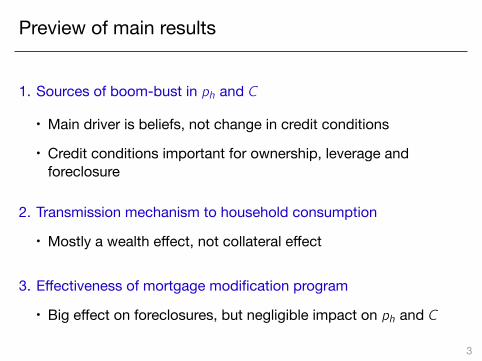
1. Sources of boom-bust in ph and C
• Main driver is beliefs, not change in credit conditions
• Credit conditions important for ownership, leverage andforeclosure
2. Transmission mechanism to household consumption
• Mostly a wealth effect, not collateral effect
3. Effectiveness of mortgage modification program
• Big effect on foreclosures, but negligible impact on ph and C
3

Preview of main results
1. Sources of boom-bust in ph and C
• Main driver is beliefs, not change in credit conditions
• Credit conditions important for ownership, leverage andforeclosure
2. Transmission mechanism to household consumption
• Mostly a wealth effect, not collateral effect
3. Effectiveness of mortgage modification program
• Big effect on foreclosures, but negligible impact on ph and C
3

Model
Model
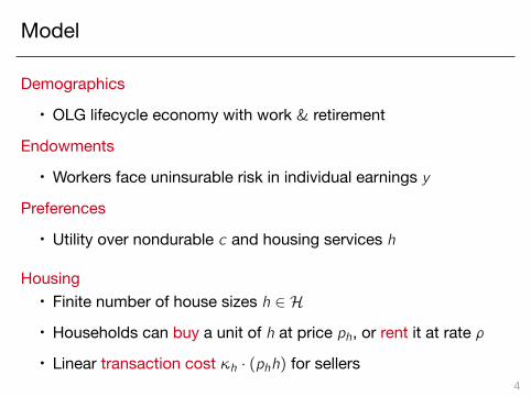
Demographics
• OLG lifecycle economy with work & retirement
Endowments
• Workers face uninsurable risk in individual earnings y
Preferences
• Utility over nondurable c and housing services h
Housing• Finite number of house sizes h ∈ H
• Households can buy a unit of h at price ph, or rent it at rate ρ
• Linear transaction cost κh · (phh) for sellers4

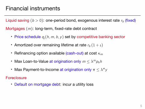
Financial instruments
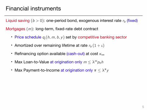
Liquid saving (b > 0): one-period bond, exogenous interest rate rb (fixed)
Mortgages (m): long-term, fixed-rate debt contract
• Price schedule qj(h,m, b, y) set by competitive banking sector
• Amortized over remaining lifetime at rate rb (1 + ι)
• Refinancing option available (cash-out) at cost κm
• Max Loan-to-Value at origination only m ≤ λmphh
• Max Payment-to-Income at origination only π ≤ λπy
Foreclosure• Default on mortgage debt: incur a utility loss
HELOCs (b < 0)
• One-period borrowing (b ≥ −λbphh), at rate rb (1 + ι), non-defaultable
• Collateralized by housing, b ≥ −λbphh
5
Financial instruments
Liquid saving (b > 0): one-period bond, exogenous interest rate rb (fixed)
Mortgages (m): long-term, fixed-rate debt contract
• Price schedule qj(h,m, b, y) set by competitive banking sector
• Amortized over remaining lifetime at rate rb (1 + ι)
• Refinancing option available (cash-out) at cost κm
• Max Loan-to-Value at origination only m ≤ λmphh
• Max Payment-to-Income at origination only π ≤ λπy
Foreclosure• Default on mortgage debt: incur a utility loss
HELOCs (b < 0)
• One-period borrowing (b ≥ −λbphh), at rate rb (1 + ι), non-defaultable
• Collateralized by housing, b ≥ −λbphh
5
Closing the model
Final good sector• Y = ZN̄ → w = Z
Construction sector• Labor + housing permits→ aggregate housing investmentsI(ph)
Rental sector• Buys housing from sellers and rents them out, or vice-versa,
sells rental units to home buyers• Operating cost ψ per unit of housing owned and rented out• Zero-profit condition yields equilibrium rental rate ρ
Government• Taxes workers (with mortgage interest deduction) and
properties, sells land permits, and pays SS benefits to retirees6

Aggregate shocks
1. Aggregate labor income: Z
2. Credit conditions: (i) credit limits (λm, λb, λπ)(ii) intermediation wedge ι
3. Beliefs / News about future housing demand:Three regimes for ϕ (share of housing services in u):
(a) ϕL: low housing share and unlikely transition to ϕH(b) ϕ∗L: low housing share and likely transition to ϕH(c) ϕH: high housing share
Boom-Bust: shift from (a) to (b), and back to (a)
7
Aggregate shocks
1. Aggregate labor income: Z
2. Credit conditions: (i) credit limits (λm, λb, λπ)(ii) intermediation wedge ι
3. Beliefs / News about future housing demand:Three regimes for ϕ (share of housing services in u):
(a) ϕL: low housing share and unlikely transition to ϕH(b) ϕ∗L: low housing share and likely transition to ϕH(c) ϕH: high housing share
Boom-Bust: shift from (a) to (b), and back to (a)7

Parameterization
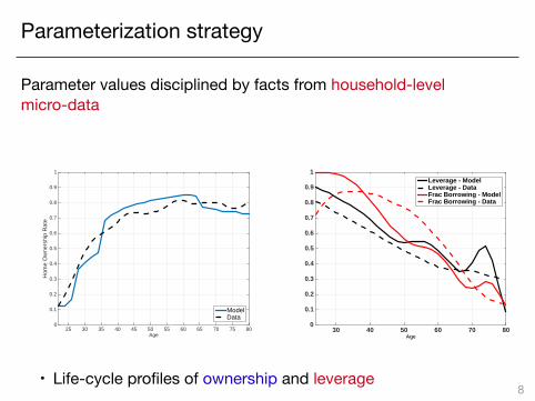
Parameterization strategy
Parameter values disciplined by facts from household-levelmicro-data
Age25 30 35 40 45 50 55 60 65 70 75 80
Hom
e O
wne
rshi
p R
ate
0
0.1
0.2
0.3
0.4
0.5
0.6
0.7
0.8
0.9
1
ModelData
Age30 40 50 60 70 80
0
0.1
0.2
0.3
0.4
0.5
0.6
0.7
0.8
0.9
1Leverage - ModelLeverage - DataFrac Borrowing - ModelFrac Borrowing - Data
• Life-cycle profiles of ownership and leverage8

Parameterization strategy
Parameter values disciplined by facts from household-levelmicro-data
• Distributional stats: mortgages, housing wealth, renters, andconsumption
Moment Empirical value Model ValueFraction homeowners w/ mortgage 0.66 0.57
Aggr. mortgage debt / housing value 0.42 0.36
P10 LTV ratio for mortgagors 0.15 0.14
P50 LTV ratio for mortgagors 0.57 0.59
P90 LTV ratio for mortgagors 0.92 0.92
Aggr. home-ownership rate 0.66 0.67
P10 house value / earnings 0.90 1.0
P50 house value / earnings 2.1 2.0
P90 house value / earnings 5.5 4.5
Avg.-size owned house / rented 1.5 1.4
Avg. earnings owners / renters 2.05 2.02
BPP consumption insurance coef 0.36 0.43 8

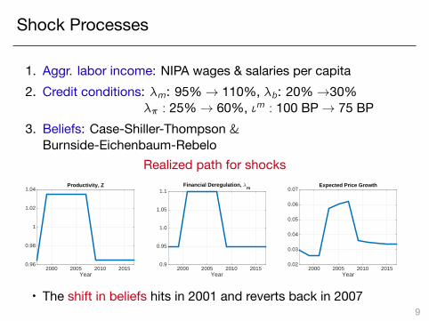
Shock Processes
1. Aggr. labor income: NIPA wages & salaries per capita2. Credit conditions: λm: 95%→ 110%, λb: 20%→30%
λπ : 25%→ 60%, ιm : 100 BP→ 75 BP3. Beliefs: Case-Shiller-Thompson &
Burnside-Eichenbaum-Rebelo
Realized path for shocks
Year2000 2005 2010 2015
0.96
0.98
1
1.02
1.04Productivity, Z
Year2000 2005 2010 2015
0.9
0.95
1.0
1.05
1.1Financial Deregulation, 6
m
Year2000 2005 2010 2015
0.02
0.03
0.04
0.05
0.06
0.07Expected Price Growth
• The shift in beliefs hits in 2001 and reverts back in 2007
9
Shock Processes
1. Aggr. labor income: NIPA wages & salaries per capita2. Credit conditions: λm: 95%→ 110%, λb: 20%→30%
λπ : 25%→ 60%, ιm : 100 BP→ 75 BP3. Beliefs: Case-Shiller-Thompson &
Burnside-Eichenbaum-RebeloRealized path for shocks
Year2000 2005 2010 2015
0.96
0.98
1
1.02
1.04Productivity, Z
Year2000 2005 2010 2015
0.9
0.95
1.0
1.05
1.1Financial Deregulation, 6
m
Year2000 2005 2010 2015
0.02
0.03
0.04
0.05
0.06
0.07Expected Price Growth
• The shift in beliefs hits in 2001 and reverts back in 20079

Q1What caused the boom-bust in ph and C?

Consumption and house price dynamics
Year2000 2005 2010 2015
0.8
0.9
1
1.1
1.2
1.3
House Price
ModelData
Year2000 2005 2010 2015
0.95
1
1.05
1.1Consumption
10

Consumption and house price dynamics
Year2000 2005 2010 2015
0.8
0.9
1
1.1
1.2
1.3
House Price
BenchmarkBelief Only
Year2000 2005 2010 2015
0.95
1
1.05
1.1Consumption
10
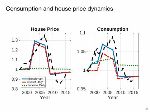
Consumption and house price dynamics
Year2000 2005 2010 2015
0.8
0.9
1
1.1
1.2
1.3
House Price
BenchmarkBelief OnlyIncome Only
Year2000 2005 2010 2015
0.95
1
1.05
1.1Consumption
10

Consumption and house price dynamics
Year2000 2005 2010 2015
0.8
0.9
1
1.1
1.2
1.3
House Price
BenchmarkBelief OnlyIncome OnlyCredit Only
Year2000 2005 2010 2015
0.95
1
1.05
1.1Consumption
10
Beliefs vs actual change in preferences
Year2000 2005 2010 2015
0.8
0.9
1
1.1
1.2
1.3
House Price
BenchmarkDemand Only
Year2000 2005 2010 2015
0.9
0.95
1
1.05
1.1Consumption
• Preference shock: similar rise in ph, but C falls!
11

Beliefs vs actual change in preferences
Year2000 2005 2010 2015
0.8
0.9
1
1.1
1.2
1.3
House Price
BenchmarkDemand Only
Year2000 2005 2010 2015
0.9
0.95
1
1.05
1.1Consumption
• Preference shock: similar rise in ph, but C falls!11

Dynamics of rent-price ratio
Year2000 2005 2010 2015
0.7
0.8
0.9
1
1.1
Benchmark
12

Dynamics of rent-price ratio
Year2000 2005 2010 2015
0.7
0.8
0.9
1
1.1
BenchmarkBelief OnlyIncome OnlyCredit Only
ρ = ψ + ph −(1− δh − τh1 + rb
)Eph
[p′h]
• Belief about future appreciation essential12

Dynamics of home ownership
Year2000 2005 2010 2015
0.95
1
1.05
1.1Benchmark
13

Dynamics of home ownership
Year2000 2005 2010 2015
0.95
1
1.05
1.1BenchmarkBelief OnlyIncome OnlyCredit Only
• Loosening of credit limits drives rise in home-ownership13

Change in home ownership by age: data and model
Age30 40 50 60
Log-
chan
ge (
rela
tive
to m
ean)
-0.05
0
0.05
0.1
0.15Boom
DataModel
Age30 40 50 60
Log-
chan
ge (
rela
tive
to m
ean)
-0.15
-0.1
-0.05
0
0.05Bust
DataModel
• It’s the young who go in/out of housing market14

Dynamics of leverage and foreclosure
Year2000 2005 2010 2015
0.8
1
1.2
1.4
1.6
1.8Leverage
Year2000 2005 2010 2015
0
0.01
0.02
0.03
0.04Foreclosure rate
Benchmark
15

Dynamics of leverage and foreclosure
Year2000 2005 2010 2015
0.8
1
1.2
1.4
1.6
1.8Leverage
Year2000 2005 2010 2015
0
0.01
0.02
0.03
0.04Foreclosure rate
BenchmarkBelief OnlyIncome OnlyCredit Only
• Credit loosening is key for constant leverage pre-boom• Interaction belief-credit important for foreclosure
15

Why credit shock does not affect ph
• Max LTV/PTI ratios affect housing demand if renters (extensivemargin) or home-owners (intensive margin) are constrained inhousing choice
1. UP: Rental market relaxes these constraints
2. DOWN: Long-term mortgage debt relaxes these constraints
16

Why credit shock does not affect ph
• Max LTV/PTI ratios affect housing demand if renters (extensivemargin) or home-owners (intensive margin) are constrained inhousing choice
1. UP: Rental market relaxes these constraints
2. DOWN: Long-term mortgage debt relaxes these constraints
• Are we missing the ‘credit supply’ aspect of the shock, i.e.cheap credit flowing to low-quality borrowers?
1. Endogenous relaxation in lending standards in response tobelief-driven boom
16

Cheaper credit for ‘low-quality’ borrowers
Leverage0.7 0.8 0.9 1 1.1
End
ogen
ous
Bor
row
ing
Rat
e (1
/qm
-1)
0.04
0.06
0.08
0.1
0.12
0.14No shocksCredit OnlyAll Shocks
• Also lenders expect prices to rise and default rates to fall17

Model Meets (New) Micro Evidence

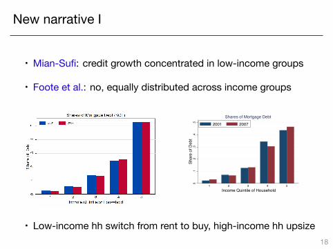
New narrative I
• Mian-Sufi: credit growth concentrated in low-income groups
• Foote et al.: no, equally distributed across income groups
0.1
.2.3
.4.5
Shar
e of
Deb
t
1 2 3 4 5 Income Quintile of Household
Shares of Mortgage Debt
2001 2007
• Low-income hh switch from rent to buy, high-income hh upsize
18
New narrative I
• Mian-Sufi: credit growth concentrated in low-income groups
• Foote et al.: no, equally distributed across income groups
0.1
.2.3
.4.5
Shar
e of
Deb
t1 2 3 4 5
Income Quintile of Household
Shares of Mortgage Debt
2001 2007
• Low-income hh switch from rent to buy, high-income hh upsize18

New narrative II
• Mian-Sufi: mortgage origin. concentrated in subprime groups
• Adelino et al.: no, equally distributed across groups
0.2
.4.6
.8Sh
are
of D
ebt
Above Median Below MedianDefault Risk
Shares of Originated Mortgage Debt2001 2007
• Young hh switch from rent to buy, older hh upsize
19

New narrative II
• Mian-Sufi: mortgage origin. concentrated in subprime groups
• Adelino et al.: no, equally distributed across groups
0.2
.4.6
.8Sh
are
of D
ebt
Above Median Below MedianDefault Risk
Shares of Originated Mortgage Debt2001 2007
• Young hh switch from rent to buy, older hh upsize19
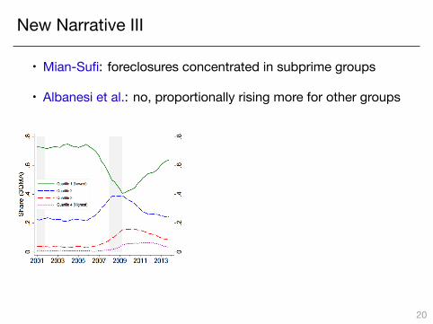
New Narrative III
• Mian-Sufi: foreclosures concentrated in subprime groups
• Albanesi et al.: no, proportionally rising more for other groups
0.2
.4.6
.81
Shar
e of
For
eclo
sure
s
2004 2006 2008 2010 2012Year
IncomeQuintile=1 IncomeQuintile=2 IncomeQuintile=3 IncomeQuintile=4 IncomeQuintile=5
• Everyone levers up, including middle-income households
20

New Narrative III
• Mian-Sufi: foreclosures concentrated in subprime groups
• Albanesi et al.: no, proportionally rising more for other groups
0.2
.4.6
.81
Shar
e of
For
eclo
sure
s2004 2006 2008 2010 2012
Year
IncomeQuintile=1 IncomeQuintile=2 IncomeQuintile=3 IncomeQuintile=4 IncomeQuintile=5
• Everyone levers up, including middle-income households20
Q2How does the fall in ph transmit to C?

Deleveraging or wealth effect in the bust?-.3
-.2-.1
0.1
Chan
ge in
Log
Con
sum
ptio
n
0 .05 .1 .15Debt as a Fraction of Total Wealth
Renters Owners
-.3-.2
-.10
.1Ch
ange
in L
og C
onsu
mpt
ion
0 .1 .2 .3 .4Housing Share of Total Wealth
Renters Owners
Deleveraging: WEAK Wealth effect: STRONG
• Consistent with Kaplan-Mitman-Violante (2016): ’Non-durableConsumption and Housing Net Worth in the Great Recession:Evidence form Easily Accessible Data’
21

Q3Could a massive debt forgiveness program
have cushioned the bust?
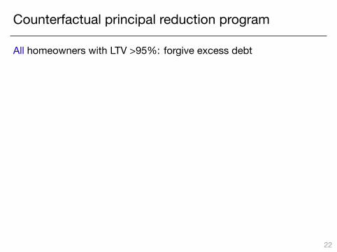
Counterfactual principal reduction program
All homeowners with LTV >95%: forgive excess debt
Year2000 2005 2010 2015
0.8
1
1.2
House Price
Bench.Mod.
Year2000 2005 2010 2015
0.95
1
1.05
1.1Consumption
Year2000 2005 2010 2015
0
0.01
0.02
0.03
Foreclosure rate
Year2000 2005 2010 2015
0.8
1
1.2
1.4
1.6
Leverage
• Beneficiaries account for small share of C + do not foreclose
22

Counterfactual principal reduction program
All homeowners with LTV >95%: forgive excess debt
Year2000 2005 2010 2015
0.8
1
1.2
House Price
Bench.Mod.
Year2000 2005 2010 2015
0.95
1
1.05
1.1Consumption
Year2000 2005 2010 2015
0
0.01
0.02
0.03
Foreclosure rate
Year2000 2005 2010 2015
0.8
1
1.2
1.4
1.6
Leverage
• Beneficiaries account for small share of C + do not foreclose22

Summary: what did we learn from the model?
1. Shift in expected house appreciation key to boom-bust in ph
2. This explanation is consistent with recent micro evidence
3. ∆ph transmits to ∆C through wealth effects
4. Principal reduction program would not have mitigated drop in C
Thanks!
23

Summary: what did we learn from the model?
1. Shift in expected house appreciation key to boom-bust in ph
2. This explanation is consistent with recent micro evidence
3. ∆ph transmits to ∆C through wealth effects
4. Principal reduction program would not have mitigated drop in C
Thanks!
23