Health and Health Inequality during the Great Recession: Evidence from the PSID*

Chenggang Wang University of Hawaii at Manoa, Department of Economics

Huixia Wang

Hunan University, School of Economics and Trade

Timothy J. Halliday+ University of Hawaii at Manoa, Department of Economics

University of Hawaii Economic Research Organization IZA

First Version: July 6, 2016

Last Update: April 25, 2017

Abstract We estimate the impact of the Great Recession of 2007-2009 on health outcomes in the United States. We show that a one percentage point increase in the unemployment rate resulted in a 7.8-8.8 percent increase in reports of poor health. Mental health was also adversely impacted and reports of chronic drinking increased. These effects were concentrated among those with strong labor force attachments. White Americans and the less educated were the most impacted demographic groups. Keywords: Great Recession, Health Behaviors, Health Outcomes, Inequality

* We thank participants at the IZA Workshop on the Social and Welfare Consequences of Unemployment in Bonn for useful feedback. + Corresponding author. Address: 2424 Maile Way; 533 Saunders Hall; Honolulu, HI 96822. E-mail: halliday@hawaii.edu

1

I. Introduction

Recessions are a major source of systematic risk to households. Because they affect large groups

of people at once, they are very difficult to insure. Moreover, due to moral hazard problems,

public insurance schemes like unemployment insurance only provide limited recourse to the

unemployed. As a consequence, recessions can have serious, adverse impacts on household and

individual welfare.

One of the more commonly studied of these potential impacts is the effect of recessions on

human health. Early work on the topic indicated that poor macroeconomic conditions raised

mortality rates substantially (e.g. Brenner 1979). However, seminal work by Ruhm (2000)

pointed out severe methodological shortcomings in this earlier work and he showed that, once

these issues are corrected, mortality rates tend to decline during recessions so that mortality rates

are actually pro-cyclical in the aggregate data.1 Improved health-related behaviors due to

relaxed time constraints and tightened budget constraints was cited as a mechanism driving these

results by Ruhm (2000, 2005), although subsequent work by Stevens, et al. (2015) suggested that

higher rates of vehicular accidents and poor nursing home staffing during robust economic times

were the primary mechanisms. Notably, more recent work by Ruhm (2015) has shown that

mortality rates for many causes of death did not decline during the Great Recession and that

mortality due to accidental poisoning actually increased. All of these studies utilize aggregate

state-level mortality and unemployment rates and so their unit of analysis is a state/time

observation.

On the other hand, studies that are based on individual-level data mostly show that health and

health-related behaviors worsen during recessions. For example, Gerdtham and Johannesson

(2003, 2005) use micro-data and show that mortality risks increase during recessions for

working-aged men. Similar evidence over the period 1984-1993 is provided for the United

States by Halliday (2014) who used the Panel Study of Income Dynamics (PSID). Browning and

1 This result has been replicated in other countries such as Canada (Ariizumi and Schirle 2012), France (Buchmueller, et al. 2007), OECD countries (Gerdtham and Ruhm 2006), Spain (Tapia Granados 2005), Germany (Neumayer 2004), and Mexico (Gonzalez and Quast 2011).

2

Heinesen (2012) use Danish administrative data and show that involuntary job displacement has

large effects on mortality, particularly, from cardiovascular disease which is similar to results in

Halliday (2014). This paper builds on earlier work by Browning, Dano, and Heinesen (2006)

that does not find any impact of displacements on hospitalization by using more outcomes

including mortality, a sample with stronger labor force attachments, as well as a substantially

larger data set. In a similar vein to these studies, Jensen and Richter (2003) showed that

pensioners who were adversely affected by a large-scale macroeconomic crisis in Russia in 1996

were 5 percent more likely to die within two years of the crisis. Related, Charles and DeCicca

(2008) use the National Health Interview Survey (NHIS) and MSA-level unemployment rates to

show that increases in the unemployment rate were accompanied by worse mental health and

increases in obesity. Hence, while the macro-based studies tend to be somewhat conflicted, the

micro-based studies indicate that the uninsured risks posed by recessions have real, adverse

impacts on human health. That said there are some micro-based studies that show that health

improves during recession e.g. Ruhm (2003) who uses a sample from the National Health

Interview Survey from 1972-1981.

In this study, we consider how the Great Recession impacted the health of Americans.

Specifically, we ask three questions. First, did the Great Recession impact health in the United

States? Second, how did it impact health? Third, who did it impact?

The Great Recession is an important episode to study since this recession was the deepest and

longest recession during the post-war period. In fact, Farber (2015) estimates that, over this

period, one in six workers lost their job at least once. From trough to peak, the unemployment

rate increased from 4.6 to 9.3 percent which is the largest increase during the post-war period.

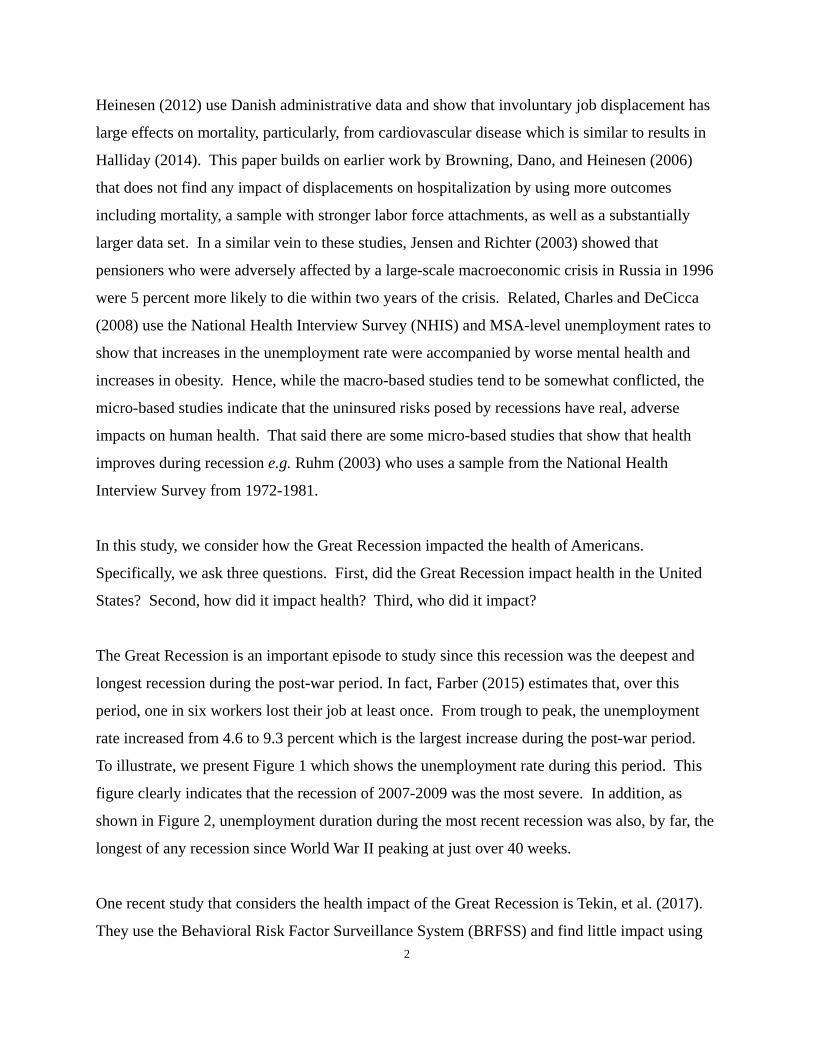
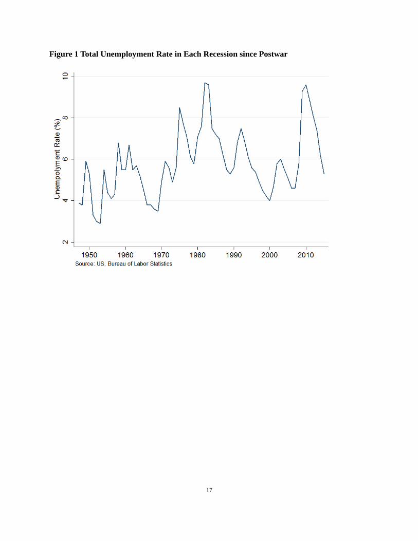
To illustrate, we present Figure 1 which shows the unemployment rate during this period. This

figure clearly indicates that the recession of 2007-2009 was the most severe. In addition, as

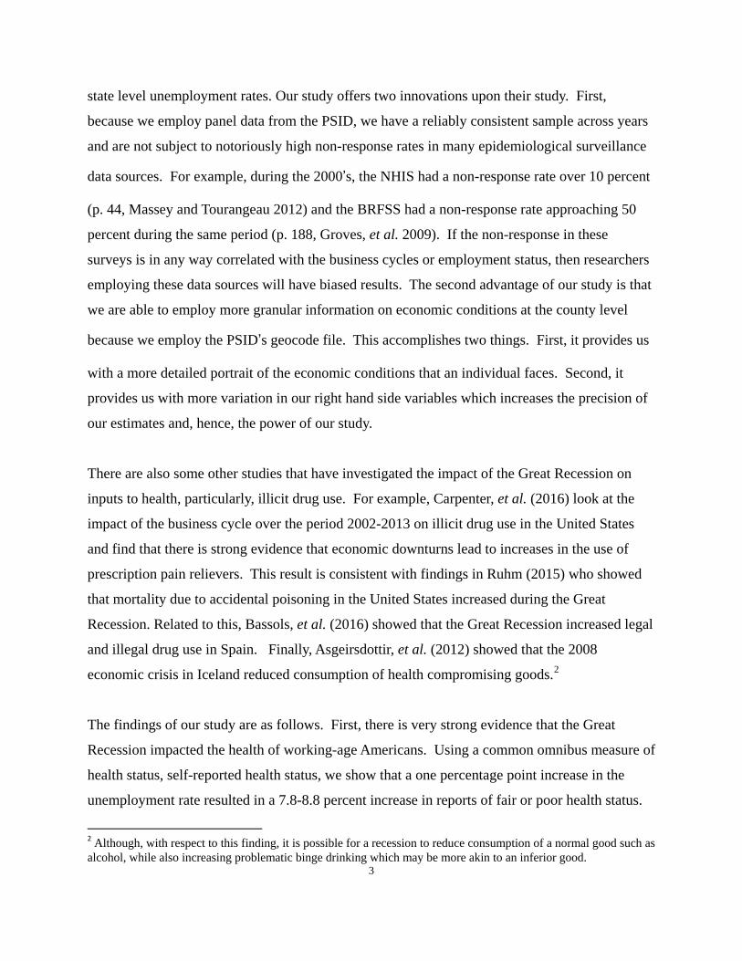
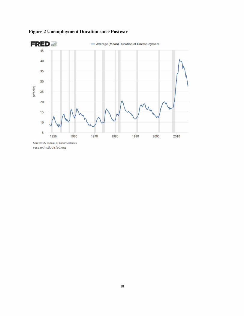
shown in Figure 2, unemployment duration during the most recent recession was also, by far, the

longest of any recession since World War II peaking at just over 40 weeks.

One recent study that considers the health impact of the Great Recession is Tekin, et al. (2017).

They use the Behavioral Risk Factor Surveillance System (BRFSS) and find little impact using

3

state level unemployment rates. Our study offers two innovations upon their study. First,

because we employ panel data from the PSID, we have a reliably consistent sample across years

and are not subject to notoriously high non-response rates in many epidemiological surveillance

data sources. For example, during the 2000’s, the NHIS had a non-response rate over 10 percent

(p. 44, Massey and Tourangeau 2012) and the BRFSS had a non-response rate approaching 50

percent during the same period (p. 188, Groves, et al. 2009). If the non-response in these

surveys is in any way correlated with the business cycles or employment status, then researchers

employing these data sources will have biased results. The second advantage of our study is that

we are able to employ more granular information on economic conditions at the county level

because we employ the PSID’s geocode file. This accomplishes two things. First, it provides us

with a more detailed portrait of the economic conditions that an individual faces. Second, it

provides us with more variation in our right hand side variables which increases the precision of

our estimates and, hence, the power of our study.

There are also some other studies that have investigated the impact of the Great Recession on

inputs to health, particularly, illicit drug use. For example, Carpenter, et al. (2016) look at the

impact of the business cycle over the period 2002-2013 on illicit drug use in the United States

and find that there is strong evidence that economic downturns lead to increases in the use of

prescription pain relievers. This result is consistent with findings in Ruhm (2015) who showed

that mortality due to accidental poisoning in the United States increased during the Great

Recession. Related to this, Bassols, et al. (2016) showed that the Great Recession increased legal

and illegal drug use in Spain. Finally, Asgeirsdottir, et al. (2012) showed that the 2008

economic crisis in Iceland reduced consumption of health compromising goods.2

The findings of our study are as follows. First, there is very strong evidence that the Great

Recession impacted the health of working-age Americans. Using a common omnibus measure of

health status, self-reported health status, we show that a one percentage point increase in the

unemployment rate resulted in a 7.8-8.8 percent increase in reports of fair or poor health status.

2 Although, with respect to this finding, it is possible for a recession to reduce consumption of a normal good such as alcohol, while also increasing problematic binge drinking which may be more akin to an inferior good.

4

This finding is robust to a number of tests. These effects were not present in a sample of older

people with weaker labor force attachments. Second, the Great Recession adversely impacted

mental health and increased drinking, although these effects were weaker than the impact on self-

rated health. Third, we detect the strongest impacts on white Americans and those with at most

12 years of schooling. In this sense our findings are consistent with important findings by Case

and Deaton (2015) who show that mortality rates of whites with less education have increased

recently.

The balance of this paper is organized as follows. In the next section, we discuss some avenues

through which the macro-economy can affect health. After that, we discuss our data. After that,

we describe our empirical methods. We then present our findings. Finally, we conclude.

II. Mechanisms

Theoretically, the impact of recessions on health and health-related behavior is ambiguous with

some effects promoting health and others adversely impacting health. This is clearly borne out

in the empirical evidence as discussed above. On the whole, the health-promoting effects of

recessions will happen via time investment in health and reduced consumption of vices provided

that they are normal goods. On the other hand, the harmful effects of recessions will happen

through increased consumption of vices if they are inferior goods, increased stress levels, or

reduced physical exertion at work if work is physically strenuous.

Health-promoting Effects

These effects have been discussed by many including Ruhm (2000). Essentially, recessions will

reduce the opportunity cost of time and reduce incomes. As a consequence, time investment in

health will increase and consumption of vices that are also normal goods will decline. Ruhm

(2005) does provide evidence for both of these channels using the BRFSS. Evidence for reduced

consumption of alcohol and other potentially harmful goods is also provided by Asgeirsdottir, et

al. (2012) and Cotti, et al. (2015). However, it is important to bear in mind that alcohol is a

normal good and, so just because some drinking declines during recessions that does not

5

preclude problematic, binge drinking from increasing.

Harmful Effects

Recessions may damage health via two channels. First, if some vices are inferior goods, then

consumption of them will increase. Moreover, although it may be the case that a good such as

alcohol is normal (e.g. Cotti, et al. (2015)), excessive use of it might be an inferior good if it is

used a coping mechanism during stressful times (e.g. Dee (2001), Davalos, et al. (2012)). A

similar argument can be made for obesity since idle time can be used for eating more and food

can also provide comfort during stressful times. Second, if people have physically strenuous

occupations, then job loss could be associated with less physical exertion.

III. Data

We utilize data from the PSID which is a national longitudinal study that collects individual-

specific information on health, demographic, and socioeconomic outcomes that is run by the

University of Michigan. The PSID began in 1968 with interviews of about 5000 families and has

continued to interview their descendants since then. To obtain county-specific information, we

use the county identifier file from the PSID.3 We utilize the 2003, 2005, 2007, 2009, 2011 and

2013 waves. We employ these waves because the 2007 and 2009 waves contain the recession

and we have two waves prior to the recession (2003 and 2005) and two waves after the recession

(2011 and 2013). Because only heads of household and their spouses were asked the health-

related questions in the survey, we limit our sample to them. We employ regional economic

indicators from the Local Area Unemployment Statistics (LAUS) of the Bureau of Labor

Statistics (BLS) which were then merged into the PSID for each year using PSID’s geocode file.

For most of the estimations, we restrict the sample to people with strong labor force attachments

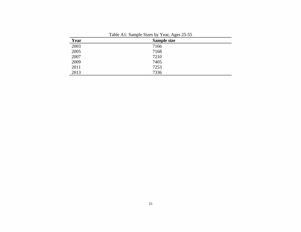
which we define to be people between ages 25 and 55. Sample sizes by year for the 25-55

3 See http://simba.isr.umich.edu/restricted/ProcessReq.aspx for details.

6

sample are reported in Table A1. In addition, we further restrict this sample by dropping people

who reported being out of the labor force, retired and disabled people, students, and housewives.

We also present some estimations for people age 65 or older. The idea for using this sample is

that this sub-sample has weaker labor force attachments and so if the impact of the recession on

health is operating through the labor market then we should see attenuated effects in this

population. In addition, because the goal of this exercise is to see if the recession impacted

people with weak labor force attachments, we included the retired, disabled, students (to the

extent that there are full-time students older than 65), and housewives as well as people who

reported being out of the labor force.

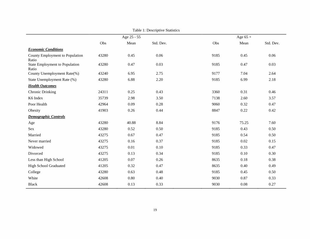
Descriptive statistics for our sample are reported in Table 1. The data can be categorized under

the rubrics: economic conditions, health outcomes, and demographic controls. The demographic

variables are fairly self-explanatory and are listed in the bottom portion of the table.

The health outcomes that we consider are drinking, mental health, self-reported health status

(SRHS), and obesity. The drinking variable that we use is an indicator for chronic drinking

which we define to be drinking several times per week or every day. For mental health

outcomes, we use the K6 Non-specific Psychological Distress scale which was also used by

Charles and DeCicca (2008). The K6 index is based on six questions designed to measure

different markers of psychological distress including reports of feelings of effortlessness,

hopelessness, restlessness, sadness, and worthlessness during the past 30 days. The K6 distress

scale is a weighted sum of these six outcomes. Kessler, et al. (2003) has shown that the K6 scale

is at least as effective as a number of other depression scales in predicting serious mental health

problems. Next, SRHS is a categorical variable that takes on integer values between one and

five where one is excellent and five is poor. We transform the SRHS variable into a binary

variable that we call poor health when SRHS equal to four or five. Halliday (2014) has shown

that SRHS is strongly predictive of mortality in the PSID. Finally, obesity is an indicator for

body mass index exceeding 30 which is the standard definition from the Centers for Disease

Control and Prevention.

The economic indicators that we consider are regional unemployment rates and

7

employment/population ratios. The county-level unemployment rate, which is our main

economic indicator, was obtained from the LAUS of the Bureau of Labor Statistics (BLS). We

collected 3,218 county unemployment rates from every other year between the years of 2003 to

2013 which corresponds to the years of our PSID sample. In our sample, the average county-

level unemployment rate was 6.95 percent with a standard deviation of 2.75 percent indicating

that there is substantial variation in county-level unemployment rates in our data. Moreover, a

regression of the county-level unemployment rate onto county fixed effects has an R2 of 47.55

percent indicating that over half of the variation of the county-level unemployment rate is within

counties which is critical for our research design’s success. In addition, for some of the

estimations, we employ regional employment/population ratios. The employment counts in the

numerators come from the LAUS and the population counts in the denominators come from the

Surveillance, Epidemiology, and End Results Program (SEER). These data have the advantage

of coming from administrative sources so should be less prone to measurement errors. The R2

from a regression of the employment/population ratio onto a set of county dummies is 42.89

percent once again indicating substantial within county variation.

IV. Methodology

To estimate the effect of the Great Recession on health outcomes and health-related behaviors,

we employ a linear regression model. If we let i denote the individual, c the county, s the state,

and y the year, the basic estimation model is:

𝐻𝐻𝑖𝑖𝑖𝑖𝑖𝑖𝑖𝑖 = 𝛽𝛽0 + 𝛽𝛽1𝑈𝑈𝑖𝑖𝑖𝑖 + 𝛽𝛽2𝑋𝑋𝑖𝑖𝑖𝑖 + 𝛿𝛿𝑖𝑖 + 𝛿𝛿𝑖𝑖 + 𝛿𝛿𝑖𝑖 ∗ 𝑡𝑡 + 𝜀𝜀𝑖𝑖𝑖𝑖𝑖𝑖𝑖𝑖. (1)

The dependent variable, 𝐻𝐻𝑖𝑖𝑖𝑖𝑖𝑖𝑖𝑖, is a health outcome or behavior. The county-specific

unemployment rate in a given year is 𝑈𝑈𝑖𝑖𝑖𝑖. The vector, 𝑋𝑋𝑖𝑖𝑖𝑖, contains individual-specific control

variables including age, gender, race, marital status, and education. We also include county and

year dummies which are denoted by 𝛿𝛿𝑖𝑖and 𝛿𝛿𝑖𝑖. Finally, we include state-specific time trends

which are denoted by 𝛿𝛿𝑖𝑖 ∗ 𝑡𝑡. We estimate two different specifications of equation (1) both with

and without the state-specific trends which has the advantage of controlling for potentially

8

confounding within state trends but the disadvantage of eliminating potentially meaningful

exogenous variation in the county-level unemployment rates. All standard errors were clustered

on the county level. Finally, we employ the weights provided by the PSID when estimating these

models.

An important feature of this research design is that we employ both county and state-specific

unemployment rates. The advantage of using county-specific indicators is that within states,

there can be considerable variation in local economic conditions, particularly, in larger states. As

such, using county-specific unemployment rates does a better job of capturing the

macroeconomic circumstances that an individual is facing. In this sense, the state-specific

unemployment rates can be viewed as error-ridden proxies for the county-specific rates. On the

other hand, as pointed out by Bartick (1996) and Hoynes (2000), there can be considerable

amounts of measurement errors in county-specific unemployment rates since these come from

surveys and imputations are often used for small counties. Note that this would tend to attenuate

estimates based on county-level unemployment rates and, so estimates based on them should be

viewed as lower bounds in the presence of classical measurement error. In addition, Lindo

(2015) has argued the spillovers in regional economic conditions across counties may result in

smaller estimates at the county level. To address these issues, we will employ economic

measures at both the county and state levels.

In this paper, we provide a formal test for the presence of spillovers. To do this, we compute an

F-test of the equality of the coefficients on the county and state unemployment rates. First, we

estimated two models, one with the county unemployment rate and one with the state

unemployment rate, as a system. This allowed us to compute the covariance between the two

parameter estimates. Next, using the two estimates from this system, we tested the null that the

two parameters from the different equations were equal. This provides a formal test of the

presence of spillovers that properly accounts for a positive covariance in the two estimates.

Our study also does a comprehensive job of controlling for heterogeneity across local labor

markets. Importantly, Tekin, et al. (2013) and Ruhm (2005) only control for state fixed effects

which only accounts for the state-level and time-invariant confounders. Clearly, the use of state

9

fixed effects may be too coarse since potential confounders such as education and health

infrastructure, culture, demographic composition, and weather may vary at a finer geographical

level. For example, Asians are about one third of the population in San Francisco whereas they

are only 0.4 percent of the population of Sierra County in California. Another example is that

within states, particularly in the South, some counties are “dry” which means that alcohol cannot

be purchased within them. Simple inclusion of state fixed effects would not account for these

within state confounders.

We also adopt a more comprehensive approach to addressing heterogeneity by including

individual fixed effects which subsume the county fixed effects. This approach has the

advantage of controlling for a greater amount of unobserved confounding variables than the

county fixed effects. However, it comes with the cost of wasting important exogenous variation

in the data as has been argued by Deaton (1997) and Angrist and Pischke (2008). It is also less

efficient and exacerbates the attenuation bias caused by measurement errors (e.g. Griliches and

Hausman 1986). As such, we view the results with the individual fixed effects as a robustness

check for our core results and we primarily focus on the results with the county fixed effects for

most of the paper.

V. Results

In this section, we answer our three research questions. First, did the Great Recession affect

health? Second, how did it affect health? Third, who did it affect?

Did the Great Recession affect health?

To address this question, we estimate equation (1) using poor health as the dependent variable.

We begin with the SRHS measure as it is a good omnibus measure of health status that exhibits

meaning time series variation. Moreover, as shown in Halliday (2014), it is highly correlated

with mortality in the PSID. The results are reported in Table 2.

Our core results are reported in the first four columns. In the first column where county fixed

10

effects are included, the estimate is 0.008 and is significant at the 1 percent level. This indicates

that a one percentage point (PP) increase in the unemployment rate results in a 0.8 PP increase in

the probability of reporting poor health. Inclusion of the state-specific trend slightly attenuates

the estimate to 0.007 but it is still highly significant. The mean of reports of poor health in our

data is 0.09, so these estimates constitute 7.8-8.8 percent increases. In the next two columns, we

replicate the specifications from the first two columns except with individual fixed effects in lieu

of county fixed effects and we see that the estimates are essentially the same.

One concern with the estimates with the county fixed effects in the first two columns is that

healthier people may selectively migrate out of depressed areas as shown in Halliday (2007). If

this were to happen then areas with high unemployment rates would have a less healthy

population due to selection as opposed to a structural effect of the macroeconomy on individual

health. One way to address this is with the inclusion of individual fixed effects as in columns

three and four. Another way to address this is to re-estimate the models in the first two columns

for a subsample of people who do not move counties while in the sample. These results are

reported in columns five and six. Both estimates are 0.007 and are still significant at the 1

percent level. This indicates that selective migration is not driving our results.

In columns seven and eight, we use the state unemployment rate instead of the county

unemployment rate. The estimates are 0.010 and 0.009 without and with state-specific trends.

While this is larger than the analogous estimates in the first two columns, the magnitude of

difference is not as large as what was found in Lindo (2015). The p-values on an F-test of the

equality of the coefficients on the county and state unemployment rates are close to unity

indicating that we cannot reject the null that the two estimates are the same. This casts doubt that

there are spillover effects in our context.

Finally, we report estimates based on county and state level employment/population ratios in the

final four columns. Of these four estimates, only the estimate using the state level ratio in

column 11 is significant. In addition, none of the corresponding estimates with the other

11

outcomes produced a significant estimate.4 Given that most of our effects appear to be operating

through the unemployment rate, we will focus on it for the duration of the paper.

How did the Great Recession affect health?

Having established that the Great Recession impacted an omnibus health measurement, we now

try and understanding how the recession impacted different components of health. To get at this,

we estimate the model in equation (1) using the K6 index, the chronic drinking indicator, and the

obesity indicator as the dependent variables.

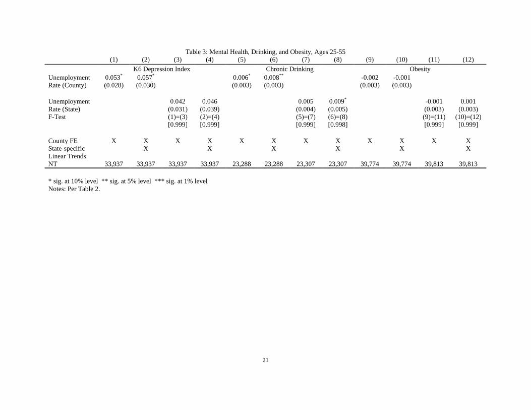
The results are reported in Table 3. First and consistent with Tefft (2011), we see in the first two

columns that mental health as proxied by the K6 scale deteriorated during the Great Recession.

The estimates without and with the state-specific trends are significant at the 10 percent level.

Note that in columns three and four where we use state level unemployment rates, both estimates

are small in magnitude and not significant, but due to their large standard errors, we cannot reject

that these estimates are equal to the estimates at the county-level. Moving on to drinking in

columns five and six, we see that a one PP increase in the county-level unemployment rate

increases the propensity to drink by 0.6-0.8 PP. From Table 1, the mean of this variable is 0.25,

so this constitutes a 2.4-3.2 percent increase. The corresponding estimates with the state

unemployment rate in columns seven and eight are similar in magnitude, although only the

estimate with the state-trends is significant at conventional levels. Once again, we do not find

any evidence of spill-overs. Finally, we look at obesity in the final four columns and see no

evidence of any effects.

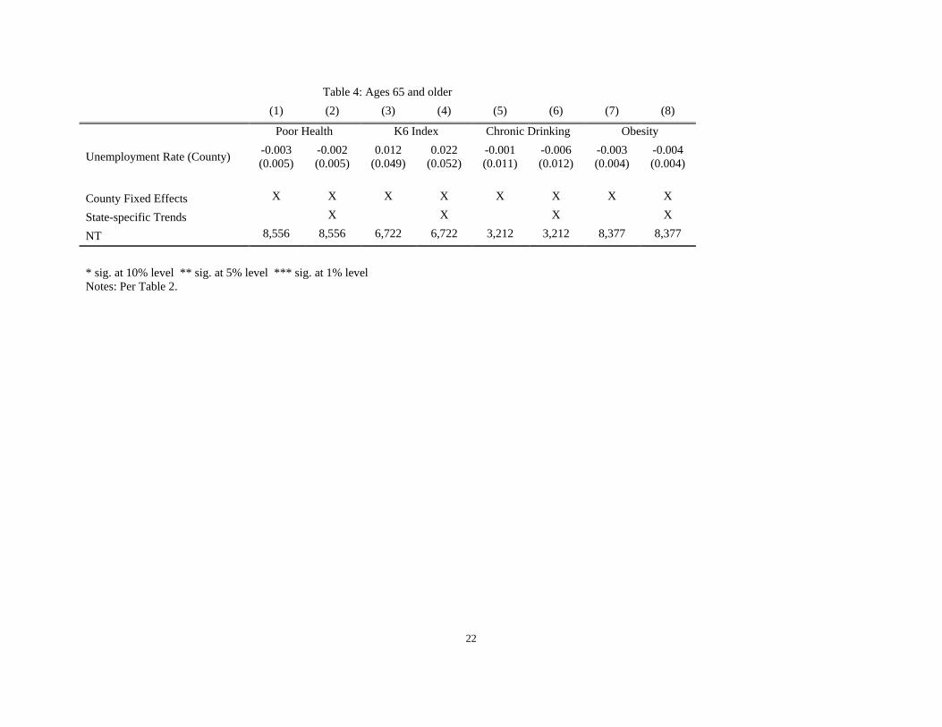
Next, in Table 4, we estimate our model for our four main outcomes on a sample that is 65 or

older that has weak labor force attachments. None of the estimates are significant. Although it is

true that due to a smaller sample size, this may be the result of less power. However, it is

interesting to note that the magnitudes also tend to be smaller than the corresponding magnitudes

in Tables 2 and 3 for the working age population, so the lack of significance is not only due to

higher standard errors. This is suggestive that our effects are operating via the labor market. 4 These results are available upon request.

12

Who was impacted the most by the Great Recession?

Finally, we investigate how the Great Recession affected different socioeconomic groups. In

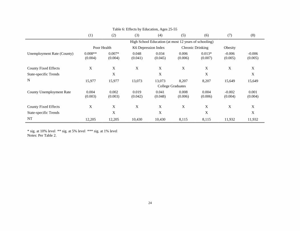
Table 5, we estimate our models separately for blacks and whites. In Table 6, we estimate the

model separately for high school and college educated people.

In Table 5, we report the results for blacks in the top panel and for whites in the bottom panel.

For blacks, we do not see any impacts on poor health or the K6 scale. In contrast, we do see

strong evidence of effects on these outcomes for whites. Based on these outcomes, the recession

had larger effects on whites. Next, looking at drinking, we see tightly estimated and significant

effects on drinking behavior for whites. For blacks, the estimates are less tightly estimated and

only the estimate with the state-trends is significant in column six. However, the magnitudes are

larger for blacks than for whites. Finally, looking at obesity in column seven which excludes the

state-trends, there is evidence of impacts on obesity albeit in opposite ways. A one PP increases

the propensity to be obese for blacks by 1.3 PP but decreases the propensity for whites by 0.5 PP.

However, these results are not robust to the inclusion of state-trends in the final column. Our

interpretation of these results is that there is stronger evidence that the recession impacted the

health of white Americans than black Americans.

Table 6 is analogous to the previous table except that now we stratify by education level. First,

we see that none of the estimates are significant for college graduates. Second, we see that, for

the high school educated, there are significant impacts on SRHS and drinking when state-trends

are included in column six. This table suggests that there is stronger evidence that the recession

had larger impacts on the less educated.

Taken together, these findings suggest that the effects of the Great Recession were

disproportionately borne by the less educated and by whites. This is consistent with important

recent findings by Case and Deaton (2015) who show that mortality of less educated whites has

risen over the period 1999-2013.

13

VI. Conclusions

In this paper, we showed that the Great Recession resulted in worse health outcomes. We built

on previous work by employing more granular information on local macroeconomic conditions

by using the geocode file from the Panel Study of Income Dynamics. Specifically, we show that

a one percentage point increase in the unemployment rate results in a 7.8-8.8 percent increase in

reports of poor health. In addition, increases in unemployment are also associated with worse

mental health and increases in reports of chronic drinking. The bulk of our effects were borne by

white and less educated people. We do not uncover any evidence that macroeconomic measures

at larger levels of aggregation have larger effects than at smaller levels and, thus, this paper

provides no evidence of spill-overs.

Our findings are not consistent with most of the aggregate studies in this literature in that we do

not find compelling evidence that any of our health measures improved during the Great

Recession. However, they are consistent with a growing body of evidence that employs

individual level data and shows that health tends to deteriorate when the economy worsens.

Moreover, we show that the people who were the most impacted were less educated, white, and

younger than age 55. This is consistent with important new findings on mortality trends in the

United States from Case and Deaton (2015).

14

References Angrist, Joshua D., and Jörn-Steffen Pischke. Mostly harmless econometrics: An empiricist's companion. Princeton university press, 2008. Ariizumi, Hideki, and Tammy Schirle. "Are recessions really good for your health? Evidence from Canada." Social Science & Medicine 74, no. 8 (2012): 1224-1231. Asgeirsdottir, Tinna Laufey, Hope Corman, Kelly Noonan, Þórhildur Ólafsdóttir, and Nancy E. Reichman. Are recessions good for your health behaviors? Impacts of the economic crisis in Iceland. No. w18233. National Bureau of Economic Research, 2012. Bartik, Timothy J. "The distributional effects of local labor demand and industrial mix: Estimates using individual panel data." Journal of Urban Economics 40, no. 2 (1996): 150-178. Bassols, Nicolau Martin, and Judit Vall Castelló. "Effects of the Great Recession on drugs consumption in Spain." Economics & Human Biology 22 (2016): 103-116. Brenner, M. Harvey. "Mortality and the national economy: A review, and the experience of England and Wales, 1936-76." The Lancet 314, no. 8142 (1979): 568-573. Browning, Martin, Anne Moller Dano, and Eskil Heinesen. "Job displacement and stress‐related health outcomes." Health economics 15, no. 10 (2006): 1061-1075. Browning, Martin, and Eskil Heinesen. "Effect of job loss due to plant closure on mortality and hospitalization." Journal of health economics 31, no. 4 (2012): 599-616. Buchmueller, Thomas C., Michel Grignon, Florence Jusot, and Marc Perronnin. Unemployment and mortality in France, 1982-2002. Centre for Health Economics and Policy Analysis, McMaster University, 2007. Carpenter, Christopher S., Chandler B. McClellan, and Daniel I. Rees. Economic Conditions, Illicit Drug Use, and Substance Use Disorders in the United States. No. w22051. National Bureau of Economic Research, 2016. Charles, Kerwin Kofi, and Philip DeCicca. "Local labor market fluctuations and health: is there a connection and for whom?." Journal of Health Economics 27, no. 6 (2008): 1532-1550. Case, Anne, and Angus Deaton. "Rising morbidity and mortality in midlife among white non-Hispanic Americans in the 21st century." Proceedings of the National Academy of Sciences 112, no. 49 (2015): 15078-15083. Cotti, Chad, Richard A. Dunn, and Nathan Tefft. "The Great Recession and Consumer Demand for Alcohol: A Dynamic Panel-Data Analysis of US Households." American Journal of Health Economics (2015).

15

Dávalos, María E., Hai Fang, and Michael T. French. "Easing the pain of an economic downturn: macroeconomic conditions and excessive alcohol consumption." Health economics 21, no. 11 (2012): 1318-1335. Deaton, Angus. The analysis of household surveys: a microeconometric approach to development policy. World Bank Publications, 1997. Dee, Thomas S. "Alcohol abuse and economic conditions: evidence from repeated cross‐sections of individual‐level data." Health economics 10, no. 3 (2001): 257-270. Farber, Henry S. Job loss in the Great Recession and its aftermath: US evidence from the displaced workers survey. No. w21216. National Bureau of Economic Research, 2015. Gerdtham, Ulf-G., and Magnus Johannesson. "A note on the effect of unemployment on mortality." Journal of health economics 22, no. 3 (2003): 505-518. Gerdtham, Ulf-G., and Magnus Johannesson. "Business cycles and mortality: results from Swedish microdata." Social science & medicine 60, no. 1 (2005): 205-218. Gerdtham, Ulf-G., and Christopher J. Ruhm. "Deaths rise in good economic times: evidence from the OECD." Economics & Human Biology 4, no. 3 (2006): 298-316. Gonzalez, Fidel, and Troy Quast. "Macroeconomic changes and mortality in Mexico." Empirical Economics 40, no. 2 (2011): 305-319. Granados, José A. Tapia. "Recessions and mortality in Spain, 1980–1997." European Journal of Population/Revue européenne de Démographie 21, no. 4 (2005): 393-422. Griliches, Zvi, and Jerry A. Hausman. "Errors in variables in panel data." Journal of econometrics 31, no. 1 (1986): 93-118. Groves, Robert M., Floyd J. Fowler Jr, Mick P. Couper, James M. Lepkowski, Eleanor Singer, and Roger Tourangeau. Survey methodology. Vol. 561. John Wiley & Sons, 2011. Halliday, Timothy J. "Business cycles, migration and health." Social Science & Medicine 64, no. 7 (2007): 1420-1424. Halliday, Timothy J. "Unemployment and Mortality: Evidence from the PSID." Social Science & Medicine 113 (2014): 15-22. Hoynes, Hilary Williamson. "Local labor markets and welfare spells: Do demand conditions matter?." Review of Economics and Statistics 82, no. 3 (2000): 351-368. Jensen, Robert T., and Kaspar Richter. "The health implications of social security failure: evidence from the Russian pension crisis." Journal of Public Economics 88, no. 1 (2004): 209-236.

16

Kessler, Ronald C., Gavin Andrews, Lisa J. Colpe, Eva Hiripi, Daniel K. Mroczek, S-LT Normand, Ellen E. Walters, and Alan M. Zaslavsky. "Short screening scales to monitor population prevalences and trends in non-specific psychological distress." Psychological medicine 32, no. 06 (2002): 959-976. Lindo, Jason M. "Aggregation and the estimated effects of economic conditions on health." Journal of health economics 40 (2015): 83-96. Massey, Douglas S., and Roger Tourangeau. The nonresponse challenge to surveys and statistics. Sage, 2012. Neumayer, Eric. "Recessions lower (some) mortality rates: evidence from Germany." Social Science & Medicine 58, no. 6 (2004): 1037-1047. Ruhm, C. J. “Are Recessions Good for Your Health?” The Quarterly journal of economics, 115, no. 2 (2000): 617-650 Ruhm, Christopher J. "Good times make you sick." Journal of health economics 22, no. 4 (2003): 637-658. Ruhm, Christopher J. "Healthy living in hard times." Journal of Health Economics 24, no. 2 (2005): 341-363. Ruhm, Christopher J. "Recessions, healthy no more?." Journal of Health Economics 42 (2015): 17-28. Stevens, Ann H., Douglas L. Miller, Marianne E. Page, and Mateusz Filipski. "The best of times, the worst of times: Understanding pro-cyclical mortality." American Economic Journal: Economic Policy 7, no. 4 (2015): 279-311. Tefft, Nathan. "Insights on unemployment, unemployment insurance, and mental health." Journal of Health Economics 30, no. 2 (2011): 258-264. Tekin, Erdal, Chandler McClellan, and Karen Jean Minyard. Health and health behaviors during the worst of times: evidence from the Great Recession. No. w19234. National Bureau of Economic Research, 2013.

17

Figure 1 Total Unemployment Rate in Each Recession since Postwar

18

Figure 2 Unemployment Duration since Postwar

19

Table 1: Descriptive Statistics Age 25 - 55 Age 65 + Obs Mean Std. Dev. Obs Mean Std. Dev. Economic Conditions County Employment to Population Ratio

43280 0.45 0.06 9185 0.45 0.06

State Employment to Population Ratio

43280 0.47 0.03 9185 0.47 0.03

County Unemployment Rate(%) 43240 6.95 2.75 9177 7.04 2.64 State Unemployment Rate (%) 43280 6.88 2.20 9185 6.99 2.18 Health Outcomes Chronic Drinking 24311 0.25 0.43 3360 0.31 0.46 K6 Index 35739 2.98 3.50 7138 2.60 3.57 Poor Health 42964 0.09 0.28 9060 0.32 0.47 Obesity 41903 0.26 0.44 8847 0.22 0.42 Demographic Controls Age 43280 40.88 8.84 9176 75.25 7.60 Sex 43280 0.52 0.50 9185 0.43 0.50 Married 43275 0.67 0.47 9185 0.54 0.50 Never married 43275 0.16 0.37 9185 0.02 0.15 Widowed 43275 0.01 0.10 9185 0.33 0.47 Divorced 43275 0.13 0.34 9185 0.10 0.30 Less than High School 41205 0.07 0.26 8635 0.18 0.38 High School Graduated 41205 0.32 0.47 8635 0.40 0.49 College 43280 0.63 0.48 9185 0.45 0.50 White 42608 0.80 0.40 9030 0.87 0.33 Black 42608 0.13 0.33 9030 0.08 0.27

20

Table 2: Poor Health (SRHS = 4 or 5), Ages 25-55 (1) (2) (3) (4) (5) (6) (7) (8) (9) (10) (11) (12) Unemployment Rate (County)

0.008*** (0.002)

0.007*** (0.002)

0.007*** (0.002)

0.008*** (0.003)

0.007*** (0.002)

0.007*** (0.003)

Unemployment Rate (State)

0.010*** (0.002)

0.009*** (0.003)

Emp/Pop Ratio (County)

0.037 (0.037)

0.033 (0.040)

Emp/Pop Ratio (State)

-0.653** (0.274)

-0.494 (0.371)

F-Test (1)=(7) [0.984]

(2)=(8) [0.995]

(9)=(11) [0.981]

(10)=(12) [0.996]

County FE X X X X X X X X X X

Individual FE X X

State-specific Linear Trends

X X X X X X

Non-mover Sample

X X

NT 40,721 40,721 40,721 40,721 25,142 25,142 40,761 40,761 40,761 40,761 40,761 40,761

* sig. at 10% level ** sig. at 5% level *** sig. at 1% level Notes: All standard errors are clustered at the county level and are reported in parentheses. All specifications control for the demographic variables listed in Table 1. We report the p-value for the F-tests in brackets.

21

Table 3: Mental Health, Drinking, and Obesity, Ages 25-55 (1) (2) (3) (4) (5) (6) (7) (8) (9) (10) (11) (12) K6 Depression Index Chronic Drinking Obesity Unemployment Rate (County)

0.053*

(0.028) 0.057*

(0.030) 0.006*

(0.003) 0.008**

(0.003) -0.002

(0.003) -0.001 (0.003)

Unemployment Rate (State)

0.042 (0.031)

0.046 (0.039)

0.005 (0.004)

0.009*

(0.005) -0.001

(0.003) 0.001

(0.003) F-Test (1)=(3)

[0.999] (2)=(4) [0.999]

(5)=(7) [0.999]

(6)=(8) [0.998]

(9)=(11) [0.999]

(10)=(12) [0.999]

County FE X X X X X X X X X X X X State-specific Linear Trends

X X X X X X

NT 33,937 33,937 33,937 33,937 23,288 23,288 23,307 23,307 39,774 39,774 39,813 39,813 * sig. at 10% level ** sig. at 5% level *** sig. at 1% level Notes: Per Table 2.

22

Table 4: Ages 65 and older (1) (2) (3) (4) (5) (6) (7) (8)

Poor Health K6 Index Chronic Drinking Obesity

Unemployment Rate (County) -0.003 (0.005)

-0.002 (0.005)

0.012 (0.049)

0.022 (0.052)

-0.001 (0.011)

-0.006 (0.012)

-0.003 (0.004)

-0.004 (0.004)

County Fixed Effects X X X X X X X X State-specific Trends X X X X NT 8,556 8,556 6,722 6,722 3,212 3,212 8,377 8,377

* sig. at 10% level ** sig. at 5% level *** sig. at 1% level Notes: Per Table 2.

23

Table 5: Effects by Race, Ages 25-55 (1) (2) (3) (4) (5) (6) (7) (8)

Blacks Poor Health K6 Depression Index Chronic Drinking Obesity Unemployment Rate (County) 0.003

(0.006) -0.001 (0.006)

-0.047 (0.073)

-0.025 (0.087)

0.012 (0.010)

0.022** (0.011)

0.013* (0.007)

0.011 (0.007)

County Fixed Effects X X X X X X X X State-specific Trends X X X X N 12,929 12,929 10,795 10,795 6,404 6,404 12,673 12,673 Whites County Unemployment Rate 0.008***

(0.002) 0.007*** (0.002)

0.061** (0.030)

0.069** (0.033)

0.007** (0.004)

0.009** (0.004)

-0.005* (0.003)

-0.003 (0.003)

County Fixed Effects X X X X X X X X State-specific Trends X X X X NT 25,538 25,538 21,238 21,238 15,870 15,870 24,936 24,936 * sig. at 10% level ** sig. at 5% level *** sig. at 1% level Notes: Per Table 2.

24

Table 6: Effects by Education, Ages 25-55 (1) (2) (3) (4) (5) (6) (7) (8)

High School Education (at most 12 years of schooling) Poor Health K6 Depression Index Chronic Drinking Obesity Unemployment Rate (County) 0.008**

(0.004) 0.007* (0.004)

0.048 (0.041)

0.034 (0.045)

0.006 (0.006)

0.013* (0.007)

-0.006 (0.005)

-0.006 (0.005)

County Fixed Effects X X X X X X X X State-specific Trends X X X X N 15,977 15,977 13,073 13,073 8,207 8,207 15,649 15,649 College Graduates County Unemployment Rate 0.004

(0.003) 0.002

(0.003) 0.019

(0.042) 0.041

(0.048) 0.008

(0.006) 0.004

(0.006) -0.002 (0.004)

0.001 (0.004)

County Fixed Effects X X X X X X X X State-specific Trends X X X X NT 12,205 12,205 10,430 10,430 8,115 8,115 11,932 11,932 * sig. at 10% level ** sig. at 5% level *** sig. at 1% level Notes: Per Table 2.

25

Table A1: Sample Sizes by Year, Ages 25-55

Year Sample size 2003 7166 2005 7168 2007 7210 2009 7405 2011 7253 2013 7336