Constraint Propagation

Christian BessiereTechnical Report LIRMM 06020CNRS/University of Montpellier

March 2006

Constraint propagation is a form of inference, not search, and assuch is more ”satisfying”, both technically and aesthetically.

—E.C. Freuder, 2005.

1 Introduction

Constraint reasoning involves various types of techniques to tackle the inherentintractability of the problem of satisfying a set of constraints. Constraint prop-agation is one of those types of techniques. Constraint propagation is centralto the process of solving a constraint problem, and we could hardly think ofconstraint reasoning without it.

Constraint propagation is a very general concept that appears under differentnames depending on both periods and authors. Among these names, we canfind constraint relaxation, filtering algorithms, narrowing algorithms, constraintinference, simplification algorithms, label inference, local consistency enforcing,rules iteration, chaotic iteration.

Constraint propagation embeds any reasoning which consists in explicitlyforbidding values or combinations of values for some variables of a problembecause a given subset of its constraints cannot be satisfied otherwise. Forinstance, in a crossword-puzzle, when you discard the words NORWAY andSWEDEN from the set of European countries that can fit a 6-digit slot becausethe second letter must be a ’R’, you propagate a constraint. In a problemcontaining two variables x1 and x2 taking integer values in 1..10, and a constraintspecifying that |x1−x2| > 5, by propagating this constraint we can forbid values5 and 6 for both x1 and x2. Explicating these ’nogoods’ is a way to reduce thespace of combinations that will be explored by a search mechanism.

The concept of constraint propagation can be found in other fields underdifferent kinds and names. (See for instance the propagation of clauses by ’unitpropagation’ in propositional calculus [40].) Nevertheless, it is in constraintreasoning that this concept shows its most accomplished form. There is noother field in which the concept of constraint propagation appears in such avariety of forms, and in which its characteristics have been so deeply analyzed.

1

In the last 30 years, the scientific community has put a lot of effort in for-malizing and characterizing this ubiquitous concept of constraint propagationand in proposing algorithms for propagating constraints. This formalizationcan be presented along two main lines: local consistencies and rules iteration.Local consistencies define properties that the constraint problem must satisfyafter constraint propagation. This way, the operational behavior is left com-pletely open, the only requirement being to achieve the given property on theoutput. The rules iteration approach, on the contrary, defines properties on theprocess of propagation itself, that is, properties on the kind/order of operationsof reduction applied to the problem.

This report does not include data-flow constraints [76], even if this line ofresearch has been the focus of quite a lot of work in interactive applications andif some of these papers speak about ‘propagation’ on these constraints [27]. Theyare indeed quite far from the techniques appearing in constraint programming.

The rest of this report is organized as follows. Section 2 contains basicdefinitions and notations used throughout the report. Section 3 formalizes allconstraint propagation approaches within a unifying framework. Sections 4–9contain the main existing types of constraint propagation. Each of these sectionspresents the basics on the type of propagation addressed and goes briefly intosharper or more recent advances on the subject.

2 Background

The notations used in this report have been chosen to support all notions pre-sented. I tried to remain on the borderline between ‘heavy abstruse notations’and ‘ambiguous definitions’, hoping I never fall too much on one side or theother of the edge.

A constraint satisfaction problem (CSP) involves finding solutions to a con-straint network, that is, assignments of values to its variables that satisfy allits constraints. Constraints specify combinations of values that given subsets ofvariables are allowed to take. In this report, we are only concerned with con-straint satisfaction problems where variables take their value in a finite domain.Without loss of generality, I assume these domains are mapped on the set

�

of integers, and so, I consider only integer variables, that is, variables with adomain being a finite subset of

�.

Definition 1 (Constraint). A constraint c is a relation defined on a sequenceof variables X(c) = (xi1 , . . . , xi|X(c)|

), called the scheme of c. c is the subset

of� |X(c)| that contains the combinations of values (or tuples) τ ∈

� |X(c)| thatsatisfy c. |X(c)| is called the arity of c. Testing whether a tuple τ satisfies aconstraint c is called a constraint check.

A constraint can be specified extensionally by the list of its satisfying tu-ples, or intensionally by a formula that is the characteristic function of theconstraint. Definition 1 allows constraints with an infinite number of satis-fying tuples. I sometimes write c(x1, . . . , xk) for a constraint c with scheme

2

X(c) = (x1, . . . , xk). Constraints of arity 2 are called binary and constraintsof arity greater than 2 are called non-binary. Global constraints are classes ofconstraints defined by a formula of arbitrary arity (see Section 9.2).

Example 2. The constraint alldifferent(x1, x2, x3) ≡ (vi 6= vj ∧vi 6= vk ∧ vj 6= vk) allows the infinite set of 3-tuples in

� 3 suchthat all values are different. The constraint c(x1, x2, x3) = {(2, 2, 3),(2, 3, 2), (2, 3, 3), (3, 2, 2), (3, 2, 3), (3, 3, 2)} allows the finite set of 3-tuples con-taining both values 2 and 3 and only them.

Definition 3 (Constraint network). A constraint network (or network) iscomposed of:

• a finite sequence of integer variables X = (x1, . . . , xn),

• a domain for X, that is, a set D = D(x1)× . . .×D(xn), where D(xi) ⊂�

is the finite set of values, given in extension,1 that variable xi can take,and

• a set of constraints C = {c1, . . . , ce}, where variables in X(cj) are in X.

Given a network N , I sometimes use XN , DN and CN to denote its sequenceof variables, its domain and its set of constraints. Given a variable xi and itsdomain D(xi), minD(xi) denotes the smallest value in D(xi) and maxD(xi) itsgreatest one. (Remember that we consider integer variables.)

In the whole report, I consider constraints involving at least two variables.This is not a restriction because domains of variables are semantically equivalentto unary constraints. They are separately specified in the definition of constraintnetwork because the domains are given extensionally whereas a constraint ccan be defined by any Boolean function on

� |X(c)| (in extension or not). Ialso consider that no variable is repeated in the scheme of a constraint. Thisrestriction could be relaxed in most cases, but it simplifies the notations. Thevocabulary of graphs is often used to describe networks. A network can indeedbe associated with a (hyper)graph where variables are nodes and where schemesof constraints are (hyper)edges.

According to Definitions 1 and 3, the variables XN of a network N and thescheme X(c) of a constraint c ∈ CN are sequences of variables, not sets. Thisis required because the order of the values matters for tuples in DN or in c.Nevertheless, it simplifies a lot the notations to consider sequences as sets whenno confusion is possible. For instance, given two constraints c and c′, X(c) ⊆X(c′) means that constraint c involves only variables that are in the scheme ofc′, whatever their ordering in the scheme. Given a tuple τ on a sequence Y ofvariables, and given a sequence W ⊆ Y , τ [W ] denotes the restriction of τ to thevariables in W , ordered according to W . Given xi ∈ Y, τ [xi] denotes the valueof xi in τ . If X(c) = X(c′), c ⊆ c′ means that for all τ ∈ c the reordering of τaccording to X(c′) satisfies c′.

1The condition on the domains given in extension can be relaxed, especially in numericalproblems where variables take values in a discretization of the reals. (See Chapter 16 in PartII of [109].)

3

Example 4. Let (1, 1, 2, 4, 5) be a tuple on Y = (x1, x2, x3, x4, x5) andW = (x3, x2, x4). τ [x3] is the value 2 and τ [W ] is the tuple (2, 1, 4). Givenc(x1, x2, x3) defined by x1 + x2 = x3 and c′(x2, x1, x3) defined by x2 + x1 ≤ x3,we have c ⊆ c′.

We also need the concepts of projection, intersection, union and join. Givena constraint c and a sequence Y ⊆ X(c), πY (c) denotes the projection of c on Y ,that is, the relation with scheme Y that contains the tuples that can be extendedto a tuple on X(c) satisfying c. Given two constraints c1 and c2 sharing thesame scheme X(c1) = X(c2), c1 ∩ c2 (resp. c1 ∪ c2) denotes the intersection(resp. the union) of c1 and c2, that is, the relation with scheme X(c1) thatcontains the tuples τ satisfying both c1 and c2 (resp. satisfying c1 or c2). Givena set of constraints {c1, . . . , ck}, on

kj=1 cj (or on {c1, . . . , ck}) denotes the join of

c1, . . . , ck, that is, the relation with scheme ∪kj=1X(cj) that contains the tuples

τ such that τ [X(cj)] ∈ cj for all j, 1 ≤ j ≤ k.Backtracking algorithms are based on the principle of assigning values to

variables until all variables are instantiated.

Definition 5 (Instantiation). Given a network N = (X, D, C),

• An instantiation I on Y = (x1, . . . , xk) ⊆ X is an assignment of valuesv1, . . . vk to the variables x1, . . . , xk, that is, I is a tuple on Y . I can bedenoted by ((x1, v1), . . . , (xk, vk)) where (xi, vi) denotes the value vi forxi.

• An instantiation I on Y is valid if for all xi ∈ Y, I [xi] ∈ D(xi).

• An instantiation I on Y is locally consistent iff it is valid and for allc ∈ C with X(c) ⊆ Y , I [X(c)] satisfies c. If I is not locally consistent, itis locally inconsistent.

• A solution to a network N is an instantiation I on X which is locallyconsistent. The set of solutions of N is denoted by sol(N).

• An instantiation I on Y is globally consistent (or consistent) if it can beextended to a solution (i.e., there exists s ∈ sol(N) with I = s[Y ]).

Example 6. Let N = (X, D, C) be a network with X =(x1, x2, x3, x4), D(xi) = {1, 2, 3, 4, 5} for all i ∈ [1..4] andC = {c1(x1, x2, x3), c2(x1, x2, x3), c3(x2, x4)} with c1(x1, x2, x3) =alldifferent(x1, x2, x3), c2(x1, x2, x3) ≡ (x1 ≤ x2 ≤ x3), andc3(x2, x4) ≡ (x4 ≥ 2 · x2). We thus have π{x1,x2}(c1) ≡ (x1 6= x2) andc1 ∩ c2 ≡ (x1 < x2 < x3). I1 = ((x1, 1), (x2, 2), (x4, 7)) is a non valid instan-tiation on Y = (x1, x2, x4) because 7 /∈ D(x4). I2 = ((x1, 1), (x2, 1), (x4, 3))is a locally consistent instantiation on Y because c3 is the only constraintwith scheme included in Y and it is satisfied by I2[X(c3)]. However, I2

is not globally consistent because it does not extend to a solution of N .sol(N) = {(1, 2, 3, 4), (1, 2, 3, 5)}.

There are many works in the constraint reasoning community that put somerestrictions on the definition of a constraint network. These restrictions can

4

have some consequences on the notions handled. I define the main restrictionsappearing in the literature and that I will use later.

Definition 7 (Normalized and binary networks).

• A network N is normalized iff two different constraints in CN do notinvolve exactly the same variables.

• A network N is binary iff for all ci ∈ CN , |X(ci)| = 2.

When a network is both binary and normalized, a constraint c(xi, xj) ∈ Cis often denoted by cij . To simplify even further the notations, cji denotes itstransposition, i.e., the constraint c(xj , xi) = {(vj , vi) | (vi, vj) ∈ cij}, and sincethere cannot be ambiguity with another constraint, I act as if cji was in C aswell.

Given two normalized networks N = (X, D, C) and N ′ = (X, D′, C ′), N tN

N ′ denotes the network N ′′ = (X, D′′, C ′′) with D′′ = D ∪ D′ and C ′′ ={c′′ | ∃c ∈ C, ∃c′ ∈ C ′, X(c) = X(c′) and c′′ = c ∪ c′}.

The constraint reasoning community often used constraints with a finitenumber of tuples, and even more, constraints that only allow valid tuples, thatis, combinations of values from the domains of the variables involved. I callthese constraints ‘embedded’.

Definition 8 (Embedded network). Given a network N and a constraintc ∈ CN , the embedding of c in DN is the constraint c with scheme X(c) suchthat c = c ∩ πX(c)(DN ). A network N is embedded iff for all c ∈ CN , c = c.

In complexity analysis, we sometimes need to refer to the size of a network.The size of a network N is equal to |XN | +

∑xi∈XN

|DN (xi)| +∑

cj∈CN‖cj‖,

where ‖c‖ is equal to |X(c)| · |c| if c is given in extension, or equal to the size ofits encoding if c is defined by a Boolean function.

3 Formal Viewpoint

This section formally characterizes the concept of constraint propagation. Theaim is essentially to relate the different notions of constraint propagation.

The constraint satisfaction problem being NP-complete, it is usually solvedby backtrack search procedures that try to extend a partial instantiation to aglobal one that is consistent. Exploring the whole space of instantiations is ofcourse too expensive. The idea behind constraint propagation is to make theconstraint network more explicit (or tighter) so that backtrack search commitsinto less inconsistent instantiations by detecting local inconsistency earlier. Ifirst introduce the following preorder on constraint networks.

Definition 9 (Preorder � on networks). Given two networks N and N ′,we say that N ′ � N iff XN ′ = XN and any instantiation I on Y ⊆ XN locallyinconsistent in N is locally inconsistent in N ′ as well.

5

From the definition of local inconsistency of an instantiation (Definition 5)I derive the following property of constraint networks ordered according to �.

Proposition 10. Given two networks N and N ′, N ′ � N iff XN ′ = XN ,DN ′ ⊆ DN ,2 and for any constraint c ∈ CN , for any tuple τ on X(c) that doesnot satisfy c, either τ is not valid in DN ′ or there exists a constraint c′ in CN ′ ,X(c′) ⊆ X(c), such that τ [X(c′)] /∈ c′.

The relation � is not an order because there can be two different networksN and N ′ with N � N ′ � N .

Definition 11 (Nogood-equivalence). Two networks N and N ′ such thatN � N ′ � N are said to be nogood-equivalent. (A nogood is a partial instan-tiation that does not lead to a solution.)

Example 12. Let N = (X, D, C) be the network with X = {x1, x2, x3},D(x1) = D(x2) = D(x3) = {1, 2, 3, 4} and C = {x1 < x2, x2 < x3, c(x1, x2, x3)}where c(x1, x2, x3) = {(111), (123), (222), (333)}. Let N ′ = (X, D, C ′) be thenetwork with C ′ = {x1 < x2, x2 < x3, c′(x1, x2, x3)}, where c′(x1, x2, x3) ={(123), (231), (312)}. The only difference between N and N ′ is that the lattercontains c′ instead of c. For any tuple τ on X(c) (resp. X(c′)) that does not sat-isfy c (resp. c′), there exists a constraint in C ′ (resp. in C) that makes τ locallyinconsistent. As a result, N � N ′ � N and N and N ′ are nogood-equivalent.

Constraint propagation transforms a network N by tightening DN , by tight-ening constraints from CN , or by adding new constraints to CN . Constraintpropagation does not remove redundant constraints, which is more a reformu-lation task. I define the space of networks that can be obtained by constraintpropagation on a network N .

Definition 13 (Tightenings of a network). The space PN of all possibletightenings of a network N = (X, D, C) is the set of networks N ′ = (X, D′, C ′)such that D′ ⊆ D and for all c ∈ C there exists c′ ∈ C ′ with X(c′) = X(c) andc′ ⊆ c.

Note that PN does not contain all networks N ′ � N . In Example 12,N ′ /∈ PN because c′ 6⊆ c. However, if N ′′ = (X, D, C ′′) with C ′′ = {x1 <x2, x2 < x3, c

′′ = c ∪ c′}, we have N ∈ PN ′′ and N ′ ∈ PN ′′ . The set of networksPN together with � forms a preordered set. The top element of PN according to� is N itself and the bottom elements are the networks with empty domains.3 InPN we are particularly interested in networks that preserve the set of solutionsof N . Psol

N denotes the subset of PN containing only the elements N ′ of PN

such that sol(N ′) = sol(N). Among the networks in PsolN , those that are the

smallest according to � have interesting properties.

2DN′ ⊆ DN because we supposed that networks do not contain unary constraints, and so,instantiations of size 1 can be made locally inconsistent only because of the domains.

3Remember that we consider that unary constraints are expressed in the domains.

6

Proposition 14 (Global consistency). Let N = (X, D, C) be a network,and GN = (X, DG, CG) be a network in Psol

N . If GN is such that for allN ′ ∈ Psol

N , GN � N ′, then any instantiation I on Y ⊆ X which is locallyconsistent in GN can be extended to a solution of N . GN is called a globallyconsistent network.

Proof. Suppose there exists an instantiation I on Y ⊆ X locally consistent inGN which does not extend to a solution. Build the network N ′ = (X, DG, CG ∪{c}) where X(c) = Y and c =

� |Y | \ {I}. N ′ ∈ PsolN because GN ∈ Psol

N and Idoes not extend to a solution of N . In addition, I is locally inconsistent in N ′.So, GN 6� N ′.

Thanks to Proposition 14 we see the advantage of having a globally consis-tent network of N . A simple brute-force backtrack search procedure applied on aglobally consistent network is guaranteed to produce a solution in a backtrack-free manner. However, globally consistent networks have a number of disad-vantages that make them impossible to use in practice. A globally consistentnetwork is not only exponential in time to compute, but in addition, its size isin general exponential in the size of N . In fact, building a globally consistentnetwork is similar to generating and storing all minimal nogoods of N . Buildinga globally consistent network is so hard that a long tradition in constraint pro-gramming is to try to transform N into an element of Psol

N as close as possibleto global consistency at reasonable cost (usually keeping polynomial time andspace). This is constraint propagation.

Rules iteration and local consistencies are two ways of formalizing constraintpropagation. Rules iteration consists in characterizing for each constraint (orset of constraints) a set of reduction rules that tighten the network. Reductionrules are sufficient conditions to rule out values (or instantiations) that haveno chance to appear in a solution. The second —and most well-known— wayof considering constraint propagation is via the notion of local consistency. Alocal consistency is a property that characterizes some necessary conditions onvalues (or instantiations) to belong to solutions. A local consistency property(denoted by Φ) is defined regardless of the domains or constraints that will bepresent in the network. A network is Φ-consistent if and only if it satisfies theproperty Φ.

It is difficult to say more about constraint propagation in completely generalterms. The preorder (PN ,�) is indeed too weak to characterize the features ofconstraint propagation. Most of the constraint propagation techniques appear-ing in constraint programming (or at least those that are used in solvers) arelimited to modifications of the domains. So, I first concentrate on this subcase,that I call domain-based constraint propagation. I will come back to the generalcase in Section 5.

Definition 15 (Domain-based tightenings). The space PND of domain-based tightenings of a network N = (X, D, C) is the set of networks in PN withthe same constraints as N , that is, N ′ ∈ PND iff XN ′ = X, DN ′ ⊆ D andCN ′ = C.

7

Proposition 16 (Partial order on networks). Given a network N , therelation � restricted to the set PND is a partial order (denoted by ≤).

(PND,≤) is a partially ordered set (poset) because given two networks N1 =(X1, D1, C1) and N2 = (X2, D2, C2), N1 ≤ N2 ≤ N1 implies that X1 = X2,C1 = C2, and D1 ⊆ D2 ⊆ D1, which means that N1 = N2. In fact, the poset(PND,≤) is isomorphic to the partial order ⊆ on DN . We are interested inthe subset Psol

ND of PND containing all the networks that preserve the set ofsolutions of N . Psol

ND has the same top element as PND, namely N itself, and aunique bottom element GND = (XN , DG, CN ), where for any xi ∈ XN , DG(xi)only contains values belonging to a solution of N , i.e., DG(xi) = π{xi}(sol(N)).Such a network was named variable-completable by Freuder [56].

Domain-based constraint propagation looks for an element in PsolND on which

the search space to explore is smaller (that is, values have been pruned fromthe domains). Since finding GND is NP-hard (consistency of N reduces tochecking non emptiness of domains in GND), domain-based constraint propa-gation usually consists of polynomial techniques that produce a network whichis an approximation of GND. The network N ′ produced by a domain-basedconstraint propagation technique always verifies GND ≤ N ′ ≤ N , that is,DG ⊆ DN ′ ⊆ DN .

Domain-based rules iteration consists in applying for each constraint c ∈ CN

a set of reduction rules that rule out values of xi that cannot appear in atuple satisfying c. Domain-based reduction rules are also named propaga-tors. For instance, if c ≡ (|x1 − x2| = k), a propagator for c on x1 can beDN(x1)← DN (x1)∩ [minDN

(x2)− k .. minDN(x2) + k]. Applying propagators

iteratively tightens DN while preserving the set of solutions of N . In otherwords, propagators slide down the poset (PND,≤) without moving out of Psol

ND.Reduction rules will be presented in Section 8. From now on, we concentrateon domain-based local consistencies. Any property Φ that specifies a necessarycondition on values to belong to solutions can be considered as a domain-basedlocal consistency. Nevertheless, we usually consider only those properties thatare stable under union.

Definition 17 (Stability under union). A domain-based property Φ isstable under union iff for any Φ-consistent networks N1 = (X, D1, C) andN2 = (X, D2, C), the network N ′ = (X, D1 ∪D2, C) is Φ-consistent.

Example 18. Let Φ be the property that guarantees that for each constraintc and variable xi ∈ X(c), at least half of the values in D(xi) belong to a validtuple satisfying c. Let X = (x1, x2) and C = {x1 = x2}. Let D1 be thedomain with D1(x1) = {1, 2} and D1(x2) = {2}. Let D2 be the domain withD2(x1) = {2, 3} and D2(x2) = {2}. (X, D1, C) and (X, D2, C) are both Φ-consistent but (X, D1 ∪ D2, C) is not Φ-consistent because among the threevalues for x1, only value 2 can satisfy the constraint x1 = x2. Φ is not stableunder union.

Stability under union brings very useful features for local consistencies.

8

Among all networks in PND that verify a local consistency Φ, there is a partic-ular one.

Theorem 19 (Φ-closure). Let N = (X, D, C) be a network and Φ be adomain-based local consistency. Let Φ(N) be the network (X, DΦ, C) whereDΦ = ∪{D′ ⊆ D | (X, D′, C) is Φ-consistent}. If Φ is stable under union,Φ(N) is Φ-consistent and is the unique network in PND such that for any Φ-consistent network N ′ ∈ PND, N ′ ≤ Φ(N). Φ(N) is called the Φ-closure of N .(By convention, we suppose (X, ∅, C) is Φ-consistent.)

Φ(N) has some interesting properties. The first one I can point out is thatit preserves the solutions: sol(Φ(N)) = sol(N). This is not the case for allΦ-consistent networks in PND.

Example 20. Let Φ be the property that guarantees that all values for allvariables can be extended consistently to a second variable. Consider thenetwork N = (X, D, C) with variables x1, x2, x3, domains all equal to {1, 2}and C = {x1 ≤ x2, x2 ≤ x3, x1 6= x3}. Let D1 be the domain withD1(x1) = D1(x2) = {1} and D1(x3) = {2}. (X, D1, C) is Φ-consistent but doesnot contain the solution (x1 = 1, x2 = 2, x3 = 2) which is in sol(N). In fact,Φ(N) = (X, DΦ, C) with DΦ(x1) = {1}, DΦ(x2) = {1, 2} and DΦ(x3) = {2}.

Computing a particular Φ-consistent network of PND can be difficult. GND

for instance, is obviously Φ-consistent for any domain-based local consistencyΦ, but it is NP-hard to compute. The second interesting property of Φ(N) isthat it can be computed by a greedy algorithm.

Proposition 21 (Fixpoint). If a domain-based consistency property Φ is sta-ble under union, then for any network N = (X, D, C), the network N ′ =(X, D′, C), where D′ is obtained by iteratively removing values that do not sat-isfy Φ until no such value exists, is the Φ-closure of N .

Corollary 22. If a domain-based consistency property Φ is polynomial to check,finding Φ(N) is polynomial as well.

By achieving (or enforcing) Φ-consistency on a network N , I mean findingthe Φ-closure Φ(N).

I define a partial order on local consistencies to express how much they per-mit to go down the poset (PND ,≤). A domain-based local consistency Φ1 isat least as strong as another local consistency Φ2 if and only if for any net-work N , Φ1(N) ≤ Φ2(N). If in addition there exists a network N ′ such thatΦ1(N

′) < Φ2(N′), then Φ1 is strictly stronger than Φ2. If there exist networks

N ′ and N ′′ such that Φ1(N′) < Φ2(N

′) and Φ2(N′′) < Φ1(N

′′), Φ1 and Φ2 areincomparable.

When networks are both normalized and embedded, stability under union, Φ-closure, and the ‘stronger’ relation between local consistencies can be extendedto local consistencies other than domain-based ones by simply replacing PND

by PN , the union on domains ∪ by the union on networks tN (see Section 2),and the partial order ≤ on PND by the preorder � on PN (see Section 5).

9

1

2

1

2 2

3

1

2

3

1

2

3

1

2

3

2 4

X1 X2 X3X1 X2 X3

X2 < X3X1 = X2

: allowed pair

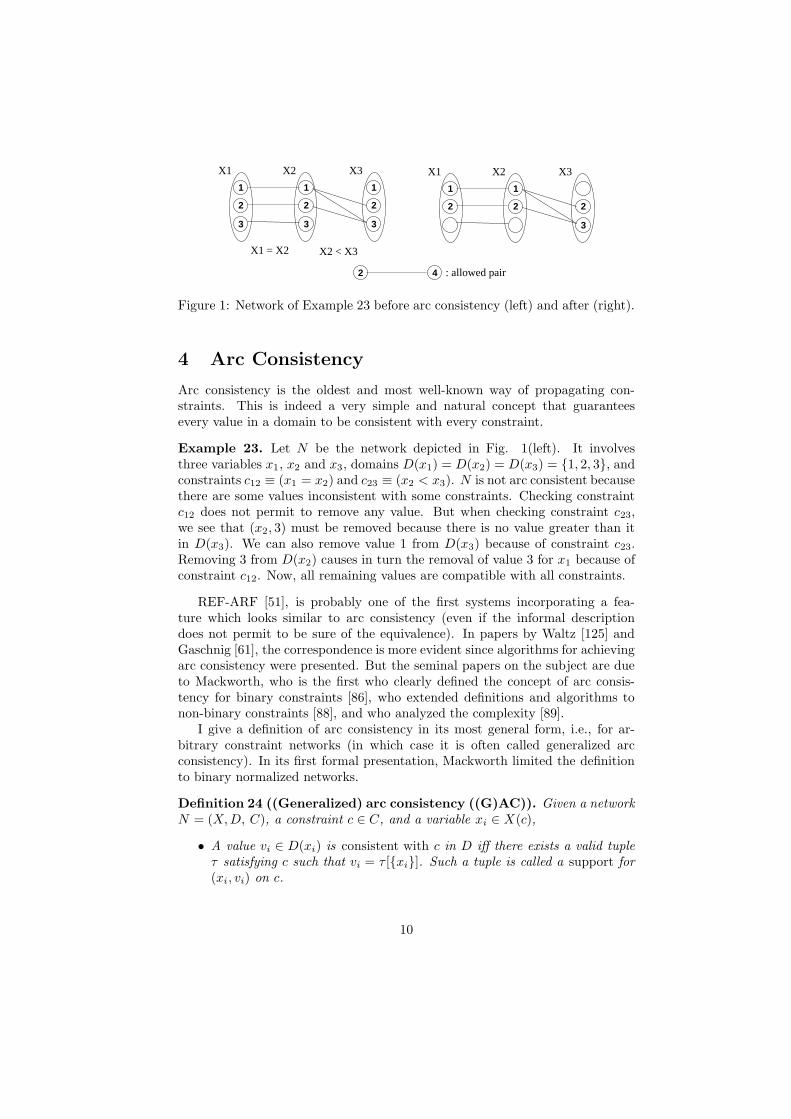
Figure 1: Network of Example 23 before arc consistency (left) and after (right).

4 Arc Consistency

Arc consistency is the oldest and most well-known way of propagating con-straints. This is indeed a very simple and natural concept that guaranteesevery value in a domain to be consistent with every constraint.

Example 23. Let N be the network depicted in Fig. 1(left). It involvesthree variables x1, x2 and x3, domains D(x1) = D(x2) = D(x3) = {1, 2, 3}, andconstraints c12 ≡ (x1 = x2) and c23 ≡ (x2 < x3). N is not arc consistent becausethere are some values inconsistent with some constraints. Checking constraintc12 does not permit to remove any value. But when checking constraint c23,we see that (x2, 3) must be removed because there is no value greater than itin D(x3). We can also remove value 1 from D(x3) because of constraint c23.Removing 3 from D(x2) causes in turn the removal of value 3 for x1 because ofconstraint c12. Now, all remaining values are compatible with all constraints.

REF-ARF [51], is probably one of the first systems incorporating a fea-ture which looks similar to arc consistency (even if the informal descriptiondoes not permit to be sure of the equivalence). In papers by Waltz [125] andGaschnig [61], the correspondence is more evident since algorithms for achievingarc consistency were presented. But the seminal papers on the subject are dueto Mackworth, who is the first who clearly defined the concept of arc consis-tency for binary constraints [86], who extended definitions and algorithms tonon-binary constraints [88], and who analyzed the complexity [89].

I give a definition of arc consistency in its most general form, i.e., for ar-bitrary constraint networks (in which case it is often called generalized arcconsistency). In its first formal presentation, Mackworth limited the definitionto binary normalized networks.

Definition 24 ((Generalized) arc consistency ((G)AC)). Given a networkN = (X, D, C), a constraint c ∈ C, and a variable xi ∈ X(c),

• A value vi ∈ D(xi) is consistent with c in D iff there exists a valid tupleτ satisfying c such that vi = τ [{xi}]. Such a tuple is called a support for(xi, vi) on c.

10

• The domain D is (generalized) arc consistent on c for xi iff all the valuesin D(xi) are consistent with c in D (that is, D(xi) ⊆ π{xi}(c∩πX(c)(D))).

• The network N is (generalized) arc consistent iff D is (generalized) arcconsistent for all variables in X on all constraints in C.

• The network N is arc inconsistent iff ∅ is the only domain tighter thanD which is (generalized) arc consistent for all variables on all constraints.

By notation abuse, when there is no ambiguity on the domain D to consider,we often say ’constraint c is arc consistent’ instead of ’D is arc consistent onc for all xi ∈ X(c)’. We also say ’variable xi is arc consistent on constraint c’instead of ’all values in D(xi) are consistent with c in D’. When a constraintcij is binary and a tuple τ = (vi, vj) supports (xi, vi) on cij , we often refer to(xj , vj) (rather than to τ itself) when we speak about a ‘support for (xi, vi)’.

Historically, many papers on constraint satisfaction made the simplifyingassumption that networks are binary and normalized. This has the advantagethat notations become much simpler (see Section 2) and new concepts are easierto present. But this had some strange effects that we must bear in mind.

First, the name ’arc consistency’ is so strongly bound to binary networks thateven if the definition is perfectly the same for both binary and non-binary con-straints, a different name has often been used for arc consistency on non-binaryconstraints. Some papers use hyper arc consistency, or domain consistency, butthe most common name is generalized arc consistency. In the following, I willuse indifferently arc consistency (AC) or generalized arc consistency (GAC),though I will use GAC when the network is explicitly non-binary.

The second strange effect of associating AC with binary normalized networksis the confusion between the notions of arc consistency and 2-consistency. (As wewill see in Section 5, 2-consistency guarantees that any instantiation of a valueto a variable can be consistently extended to any second variable.) On binarynetworks, 2-consistency is at least as strong as AC. When the binary network isnormalized, arc consistency and 2-consistency are equivalent. However, this isnot true in general. The following examples show that 2-consistency is strictlystronger than AC on non normalized binary networks and that generalized arcconsistency and 2-consistency are incomparable on arbitrary networks.

Example 25. Let N be a network involving two variables x1 and x2, withdomains {1, 2, 3}, and the constraints x1 ≤ x2 and x1 6= x2. This network is arcconsistent because every value has a support on every constraint. However, thisnetwork is not 2-consistent because the instantiation x1 = 3 cannot be extendedto x2 and the instantiation x2 = 1 cannot be extended to x1.

Let N be a network involving three variables x1, x2, and x3, with do-mains D(x1) = D(x2) = {2, 3} and D(x3) = {1, 2, 3, 4}, and the constraintalldifferent(x1, x2, x3). N is 2-consistent because every value for any vari-able can be extended to a locally consistent instantiation on any second variable.However, this network is not GAC because the values 2 and 3 for x3 do not havesupport on the alldifferent constraint.

11

4.1 Complexity of arc consistency

There are a number of questions related to GAC reasoning. It is worth analyz-ing their complexity. Bessiere et al. have characterized five questions that canbe asked about a constraint [21]. Some of the questions are more of an aca-demic nature whereas others are at the heart of propagation algorithms. Thesequestions can be asked in general, or on a particular class of constraints, such asa given global constraint (see Section 9.2). These questions can be adapted toother local consistencies that we will present in latter sections. In the following,I use the notation Problem[data] to refer to the instance of Problem withthe input ’data’.

GACSupport

Instance. A constraint c, a domain D on X(c), and a value v forvariable xi in X(c)Question. Does value v for xi have a support on c in D?

GACSupport is at the core of all generic arc consistency algorithms. GAC-

Support is generally asked for all values one by one.

IsItGAC

Instance. A constraint c, a domain D on X(c)Question. Does GACSupport[c, D, xi, v] answer ‘yes’ for eachvariable xi ∈ X(c) and each value v ∈ D(xi)?

IsItGAC has both practical and theoretical importance. If enforcing GAC ona particular constraint is expensive, we may first test whether it is necessaryor not to launch the propagation algorithm (i.e., whether the constraint is al-ready GAC). On the academic side, this question is commonly used to comparedifferent levels of local consistency.

NoGACWipeOut

Instance. A constraint c, a domain D on X(c)Question. Is there a non empty D′ ⊆ D on which IsItGAC[c, D′]answers ‘yes’?

NoGACWipeOut occurs when GAC is maintained during search by a back-track procedure. At each node in the search tree (i.e., after each instantiationof a value to a variable), we want to know if the remaining network can bemade GAC without wiping out the domain. If not, we must unassign one of thevariables already instantiated.

maxGAC

Instance. A constraint c, a domain D0 on X(c), and a domainD ⊆ D0

Question. Is (X(c), D, {c}) the arc consistent closure of(X(c), D0, {c})?

12

NoGACWipeOut

GACDomain

maxGAC

IsItGAC

GACSupport

A B : if A is NP−hard then B is NP−hard

Figure 2: Dependencies between intractability of arc consistency questions

Arc consistency algorithms (see next subsection) are asked to return the arc con-sistent closure of a network, that is, the subdomain that is GAC and any largersubdomain is not GAC. maxGAC characterizes this ‘maximality’ problem.

GACDomain

Instance. A constraint c, a domain D0 on X(c)Output. The domain D such that maxGAC[c, D0, D] answers ‘yes’

GACDomain returns the arc consistent closure, that is, the domain that a GACalgorithm computes. GACDomain is not a decision problem as it computessomething other than ‘yes’ or ‘no’.

In [20, 21], Bessiere et al. showed that all five questions are NP-hard ingeneral. In addition, they showed that on any particular class of constraints,NP-hardness of a question implies NP-hardness of other questions.

Theorem 26 (Dependencies in the NP-hardness of GAC ques-tions). Given a class C of constraints, GACSupport is NP-hard on Ciff NoGACWipeOut is NP-hard on C. GACSupport is NP-hard on Ciff GACDomain is NP-hard on C. If maxGAC is NP-hard on C thenGACSupport is NP-hard on C. If IsItGAC is NP-hard on C then maxGAC

is NP-hard on C.

A summary of the dependencies in Theorem 26 is given in Fig. 2. Notethat because each arrow from question A to question B in Fig. 2 means that Acan be rewritten as a polynomial number of calls to B, we immediately derivethat tractability of B implies tractability of A. Whereas the decision problemsGACSupport, IsItGAC, and NoGACWipeOut are in NP, maxGAC may beoutside NP. In fact, maxGAC is DP -complete in general. The DP complexityclass contains problems which are the conjunction of a problem in NP and onein coNP [101].

Assuming P 6= NP, GAC reasoning is thus not tractable in general. In fact,the best complexity that can be achieved for an algorithm enforcing GAC ona network with any kind of constraints is in O(erdr), where e is the number ofconstraints and r is the largest arity of a constraint.

13

Though not related to GAC, constraint entailment ([70]) is a sixth ques-tion that is used by constraint solvers to speed up propagation. An entailedconstraint can safely be disconnected from the network.

Entailed

Instance. A constraint c, a domain D on X(c)Question. Does IsItGAC[c, D′] answer ‘yes’ for all D′ ⊆ D?

Entailment of c on D means that D ⊆ c. Entailed is coNP-complete in general.There is no dependency between intractability of entailment and intractability ofthe GAC questions. On a class C of constraints, Entailed can be tractable andthe GAC questions intractable, or the reverse, or both tractable or intractable.

4.2 Arc consistency algorithms

Proposing efficient algorithms for enforcing arc consistency has always beenconsidered as a central question in the constraint reasoning community. A firstreason is that arc consistency is the basic propagation mechanism that is prob-ably used in all solvers. A second reason is that the new ideas that permitto improve efficiency of arc consistency can usually be applied to algorithmsachieving other local consistencies. This is why I spend some time presentingthe main algorithms that have been introduced, knowing that the techniquesinvolved can be used for other local consistencies presented in forthcoming sec-tions. I follow a chronological presentation to emphasize the incremental processthat led to the current algorithms.

4.2.1 AC3

The most well-known algorithm for arc consistency is the one proposed by Mack-worth in [86] under the name AC3. It was proposed for binary normalized net-works and actually achieves 2-consistency. It was extended to GAC in arbitrarynetworks in [88]. This algorithm is quite simple to understand. The burden ofthe general notations being not so high, I present it in its general version. (SeeAlgorithm 1.)

The main component of GAC3 is the revision of an arc, that is, the updateof a domain wrt a constraint.4 Updating a domain D(xi) wrt a constraint cmeans removing every value in D(xi) that is not consistent with c. The functionRevise(xi, c) takes each value vi in D(xi) in turn (line 2), and explores the spaceπX(c)\{xi}(D), looking for a support on c for vi (line 3). If such a support isnot found, vi is removed from D(xi) and the fact that D(xi) has been changedis flagged (lines 4–5). The function returns true if the domain D(xi) has beenreduced, false otherwise (line 6).

The main algorithm is a simple loop that revises the arcs until no changeoccurs, to ensure that all domains are consistent with all constraints. To avoidtoo many useless calls to Revise (as this is the case in the very basic AC

4The word ’arc’ comes from the binary case but we also use it on non-binary constraints.

14

Algorithm 1: AC3 / GAC3

function Revise3(in xi: variable; c: constraint): Boolean ;begin

CHANGE ← false;1

foreach vi ∈ D(xi) do2

if 6 ∃τ ∈ c ∩ πX(c)(D) with τ [xi] = vi then3

remove vi from D(xi);4

CHANGE ← true;5

return CHANGE ;6

end

function AC3/GAC3(in X: set): Boolean ;begin

/* initalisation */;Q← {(xi, c) | c ∈ C, xi ∈ X(c)};7

/* propagation */;while Q 6= ∅ do8

select and remove (xi, c) from Q;9

if Revise(xi, c) then10

if D(xi) = ∅ then return false ;11

else Q← Q ∪ {(xj , c′) | c′ ∈ C ∧ c′ 6= c ∧ xi, xj ∈ X(c′) ∧ j 6= i};12

return true ;13

end

algorithms such as AC1 or AC2), the algorithm maintains a list Q of all thepairs (xi, c) for which we are not guaranteed that D(xi) is arc consistent onc. In line 7, Q is filled with all possible pairs (xi, c) such that xi ∈ X(c).Then, the main loop (line 8) picks the pairs (xi, c) in Q one by one (line 9)and calls Revise(xi, c) (line 10). If D(xi) is wiped out, the algorithm returnsfalse (line 11). Otherwise, if D(xi) is modified, it can be the case that a valuefor another variable xj has lost its support on a constraint c′ involving bothxi and xj . Hence, all pairs (xj , c

′) such that xi, xj ∈ X(c′) must be put againin Q (line 12). When Q is empty, the algorithm returns true (line 13) as weare guaranteed that all arcs have been revised and all remaining values of allvariables are consistent with all constraints

Proposition 27 (GAC3). GAC3 is a sound and complete algorithm forachieving arc consistency that runs in O(er3dr+1) time and O(er) space, wherer is the greatest arity among constraints.

McGregor proposed a different way of propagating constraints in AC3, thatwas later named variable-oriented, as opposed to the arc-oriented propagationpolicy of AC3 [91]. Instead of putting in Q all arcs that should be revised aftera change in D(xi) (line 12), we simply put xi. Q contains variables for which achange in their domain has not yet been propagated. When picking a variable xj

from Q, the algorithm revises all arcs (xi, c) that could lead to further deletionsbecause of xj . The implementation of this version of AC3 is simpler because

15

the elements in Q are just variables. But this less precise information has adrawback. An arc can be revised several times whereas the classical AC3 wouldrevise it once. For instance, imagine a network containing a constraint c withscheme (x1, x2, x3). If a modification occurs on x2 because of a constraint c′,AC3 puts (x1, c) and (x3, c) in Q. If a modification occurs on x3 because ofanother constraint c′′ while the previous arcs have not yet been revised, AC3adds (x2, c) to Q but not (x1, c) which is already there. The same scenario withMcGregor’s version will put x2 and x3 in Q. Picking them from Q in sequence,it will revise (x1, c) and (x3, c) because of x2, and (x1, c) and (x2, c) becauseof x3. (x1, c) has been revised twice. Boussemart et al. proposed a modifiedversion of McGregor’s algorithm that solves this problem by storing a counterfor each arc [28].

From now on, I switch to binary normalized networks because most of theliterature used this simplification, and I do not want to make assumptions onwhich extension the authors would have chosen. Nevertheless, the ideas alwaysallow extensions to non normalized binary networks, and most of the time tonetworks with non-binary constraints.

Corollary 28 (AC3). AC3 achieves arc consistency on binary networks inO(ed3) time and O(e) space.

The time complexity of AC3 is not optimal. The fact that function Revise

does not remember anything about its computations to find supports for valuesleads AC3 to do and redo many times the same constraint checks.

Example 29. Let x, y and z be three variables linked by the constraints c1 ≡x ≤ y and c2 ≡ y 6= z, with D(x) = D(y) = {1, 2, 3, 4} and D(z) = {3}.Revise(x, c1) requires 1 constraint check for finding support for (x, 1), 2 checksfor (x, 2), etc., so a total of 1+2+3+4=10 constraint checks to prove that allvalues in D(x) are consistent with c1. All these constraint checks are depictedas arrows in Fig. 3.a. Revise(y, c1) requires 4 additional constraint checksto prove that y values are all consistent with (x, 1). Revise(y, c2) requires 4constraint checks to prove that all values are consistent with (z, 3) except (y, 3)which is removed. Hence, the arc (x, c1) is put in Q. Revise(z, c2) requires 1single constraint check to prove that (z, 3) is consistent with (y, 1).

When (x, c1) is picked from Q, a new call to Revise(x, c1) is launched (Fig.3.b). It requires 1+2+3+3=9 checks, among which only ((x, 3), (y, 4)) has notalready been performed at the first call.

4.2.2 AC4

AC3 being non optimal, Mohr and Henderson proposed AC4 to improve thetime complexity [92, 93]. The idea of AC4, as opposed to AC3, is to store alot of information. AC3 performs the minimum amount of work inside a callto Revise, just ensuring that all remaining values of xi are consistent with cand memorizing nothing. The price to pay is to redo much of the work if thesame Revise is recalled. AC4 stores the maximum amount of information in a

16

1

4

3

2

1

4

3

23

Initialisation: Revise (X,c1), (Y,c1), (Y,c2), (Z,c2)

X Y ZY = ZX <= Y

4 + 1 constraint10 + 4 constraintchecks checks

c2:c1:

1

4

3

23

1

4

3

2

X Y ZY = ZX <= Y

checks

Propagation: Revise (X,c1)

9 constraint

c1: c2:

(a) (b)

Figure 3: AC3 behavior depicted on Example 29. (Plain arrows represent posi-tive constraint checks whereas dashed arrows represent negative ones.)

preprocessing step in order to avoid redoing several times the same constraintcheck during the propagation of deletions.

AC4 is presented in Algorithm 2. It computes a counter counter[xi, vi, xj ]for each triple (xi, vi, xj) where cij ∈ C and vi ∈ D(xi). This counter will finallysay how many supports vi has on cij . AC4 also builds lists S[xj , vj ] containingall values that are supported by (xj , vj) on cij . In the initialization phase, AC4performs all possible constraint checks on all constraints. Each time a supportvj ∈ D(xj) is found for (xi, vi) on cij , counter[xi, vi, xj ] is incremented, and(xi, vi) is added to S[xj , vj ] (lines 3 and 5). Each time a value is found withoutsupport on a constraint, it is removed from the domain and put in the list Qfor future propagation (line 4). Once the initialization is finished, we enter thepropagation loop (line 7), which consists in propagating the consequences ofthe removals of values in Q. For each value (xj , vj) picked from Q (line 8),we just need to decrement counter[xi, vi, xj ] for each value (xi, vi) ∈ S[xj , vj ]to maintain the counters up to date (line 11). If counter[xi, vi, xj ] reacheszero, this means that (xj , vj) was the last support for (xi, vi) on cij . (xi, vi) isremoved and put in the list Q (lines 12 and 13). When Q is empty, we knowthat all values remaining in the domains have a non zero counter on all theirconstraints, and so are arc consistent.

AC4 is the first algorithm in a category later named ‘fine-grained’ algorithms[127] because they perform propagations (via list Q) at the level of values.‘Coarse-grained’ algorithms, such as AC3, propagate at the level of constraints(or arcs), which is less precise and can involve unnecessary work.

Proposition 30 (AC4). AC4 achieves arc consistency on binary normalizednetworks in O(ed2) time and O(ed2) space. Its time complexity is optimal.

Example 31. Take again the network in Example 29 with constraints c1 ≡x ≤ y and c2 ≡ y 6= z, and domains D(x) = D(y) = {1, 2, 3, 4} and D(z) = {3}.In its initialization phase, AC4 first counts the number of supports of each

17

Algorithm 2: AC4

function AC4(in X: set): Boolean ;begin

/* initialization */;Q← ∅; S[xj , vj ] = 0, ∀vj ∈ D(xj), ∀xj ∈ X;1

foreach xi ∈ X, cij ∈ C, vi ∈ D(xi) do2

initialize counter[xi, vi, xj ] to |{vj ∈ D(xj) | (vi, vj) ∈ cij}|;3

if counter[xi, vi, xj ] = 0 then remove vi from D(xi) and add (xi, vi) to4

Q;add (xi, vi) to each S[xj , vj ] s.t. (vi, vj) ∈ cij ;5

if D(xi) = ∅ then return false ;6

/* propagation */;while Q 6= ∅ do7

select and remove (xj , vj) from Q;8

foreach (xi, vi) ∈ S[xj , vj ] do9

if vi ∈ D(xi) then10

counter[xi, vi, xj ] = counter[xi, vi, xj ]− 1;11

if counter[xi, vi, xj ] = 0 then12

remove vi from D(xi); add (xi, vi) to Q;13

if D(xi) = ∅ then return false ;14

return true ;15

end

value on each constraint and builds the lists of supported values. Thus, in itsinitialization, AC4 performs all possible constraint checks for every value in eachdomain, that is, 4 · 4 = 16 constraint checks on c1 and 4 · 1 = 4 on c2.

5 At theend of this phase, the data structures are the following:

counter[x, 1, y] = 4 counter[y, 1, x] = 1 counter[y, 1, z] = 1counter[x, 2, y] = 3 counter[y, 2, x] = 2 counter[y, 2, z] = 1counter[x, 3, y] = 2 counter[y, 3, x] = 3 counter[y, 3, z] = 0counter[x, 4, y] = 1 counter[y, 4, x] = 4 counter[y, 4, z] = 1

counter[z, 3, y] = 3

S[x, 1] = {(y, 1), (y, 2), (y, 3), (y, 4)} S[y, 1] = {(x, 1), (z, 3)}S[x, 2] = {(y, 2), (y, 3), (y, 4)} S[y, 2] = {(x, 1), (x, 2), (z, 3)}S[x, 3] = {(y, 3), (y, 4)} S[y, 3] = {(x, 1), (x, 2), (x, 3)}S[x, 4] = {(y, 4)} S[y, 4] = {(x, 1), (x, 2), (x, 3), (x, 4), (z, 3)}

S[z, 3] = {(y, 1), (y, 2), (y, 4)}

The only counter equal to zero is counter[y, 3, z]. So, (y, 3) is removed andAC4 enters the propagation loop with (y, 3) in Q. When (y, 3) is picked fromQ, S[y, 3] is traversed and counter[x, 1, y], counter[x, 2, y],counter[x, 3, y] are

5In the original version of AC4 presented in [92], each constraint cij is processed twice(once for xi and once for xj), which gives 32 constraint checks on c1 and 8 on c2). Thegeneral version presented in [93] processes each constraint only once, updating all relevantcounters and lists at the same time.

18

decremented (because (x, 1), (x, 2), (x, 3) are in S[y, 3]). None of these countersare equal to zero and no value is removed. We observe that the propagation ofthe deletion of (y, 3) did not require any constraint check. It required traversalsof S[..] lists and updates of counters.

While being optimal in time, AC4 does not only suffer from its high spacecomplexity. Its very expensive initialization phase can be by itself prohibitivein time. In fact, we can informally say that AC4 has optimal worst-case timecomplexity but it almost always reaches this worst-case. Wallace discussed thisissue in [121]. In addition, even when the initialization phase has finished, AC4maintains a so accurate view of the process that it spends a lot of effort updatingits counters and traversing its lists. This is visible in Example 31, where theremoval of (y, 3) provoked traversal of S[y, 3] and counter updates, whereas allremaining values had supports.

The non-binary version GAC4, proposed by Mohr and Masini in [93], is inthe optimal O(erdr) time complexity given in Section 4.1, where r is the greatestarity among all constraints.

4.2.3 AC6

Bessiere and Cordier proposed AC6, a compromise between AC3 laziness andAC4 eagerness [15, 14]. The motivation behind AC6 is both to keep the optimalworst-case time complexity of AC4 and to stop the search for support for a valueon a constraint as soon as the first support is found, as done in Revise of AC3.In addition, AC6 maintains a data structure lighter than AC4. In fact, the ideain AC6 is not to count all the supports a value has on a constraint, but just toensure that it has at least one. AC6 only needs lists S, where S[xj , vj ] containsall values for which (xj , vj) is the current support. That is, (xi, vi) ∈ S[xj , vj ]if and only if vj was the first support found for vi on cij .

6

In Algorithm 3, AC6 looks for one support (the first one or smallest one withrespect to the ordering on integers) for each value (xi, vi) on each constraint cij

(line 3). When (xj , vj) is found as the smallest support of (xi, vi) on cij , (xi, vi)is added to S[xj , vj ], the list of values currently having (xj , vj) as smallestsupport (line 4). If no support is found, (xi, vi) is removed and is put in thelist Q for future propagation (line 5). The propagation loop (line 7) consistsin propagating the consequences of the removal of values in Q. When (xj , vj)is picked from Q, AC6 looks for the next support on cij for each value (xi, vi)in S[xj , vj ]. Instead of starting at minD(xj) as AC3 would do, it starts at thevalue of D(xj) following vj (line 11). If a new support v′

j is found, (xi, vi) isput in S[xj , v

′j ] (line 12). Otherwise, (xi, vi) is removed and put in Q (line 14).

When Q is empty, we know that all remaining values have a current support onevery constraint.

Like AC4, AC6 is a fine-grained algorithm because it propagates along val-ues. It does not reconsider constraint cij when the removed value (xj , vj) has no

6A similar technique, called ’watch literals’, has independently been proposed by Moskewiczet al. for efficient unit propagation in their Chaff solver for SAT [97].

19

Algorithm 3: AC6

function AC6(in X: set): Boolean ;begin

/* initialization */;Q← ∅; S[xj , vj ] = 0, ∀vj ∈ D(xj), ∀xj ∈ X;1

foreach xi ∈ X, cij ∈ C, vi ∈ D(xi) do2

vj ← smallest value in D(xj) s.t. (vi, vj) ∈ cij ;3

if vj exists then add (xi, vi) to S[xj , vj ];4

else remove vi from D(xi) and add (xi, vi) to Q;5

if D(xi) = ∅ then return false ;6

/* propagation */;while Q 6= ∅ do7

select and remove (xj , vj) from Q;8

foreach (xi, vi) ∈ S[xj , vj ] do9

if vi ∈ D(xi) then10

v′

j ← smallest value in D(xj) greater than vj s.t. (vi, vj) ∈ cij ;11

if v′

j exists then add (xi, vi) to S[xj , v′

j ];12

else13

remove vi from D(xi); add (xi, vi) to Q;14

if D(xi) = ∅ then return false ;15

return true ;16

end

chance to provoke another removal in D(xi), that is, when D(xi)∩S[xj , vj ] = ∅.

Proposition 32 (AC6). AC6 achieves arc consistency on binary normalizednetworks in O(ed2) time and O(ed) space.

Example 33. I show what the data structures of AC6 are on the example usedfor AC3 (Example 29) and for AC4 (Example 31), i.e., constraints c1 ≡ x ≤ yand c2 ≡ y 6= z and domains D(x) = D(y) = {1, 2, 3, 4} and D(z) = {3}. Inits initialization phase, AC6 looks for one support (the smallest) for each valueon each constraint and stores the fact that a value (xj , vj) has been found assupporting (xi, vi) by adding (xi, vi) to S[xj , vj ]. Thus, in its initialization,AC6 performs the same number of constraint checks as AC3, namely 10+4 onc1 and 4+1 on c2. At the end of this phase, the data structures are the following,

S[x, 1] = {(y, 1), (y, 2), (y, 3), (y, 4)} S[y, 1] = {(x, 1), (z, 3)}S[x, 2] = {} S[y, 2] = {(x, 2)}S[x, 3] = {} S[y, 3] = {(x, 3)}S[x, 4] = {} S[y, 4] = {(x, 4)}

S[z, 3] = {(y, 1), (y, 2), (y, 4)}

and the list Q contains (y, 3) which has been removed. When AC6 enters thepropagation loop it pops (y, 3) from Q, S[y, 3] is traversed and a new supportgreater than 3 is sought for (x, 3). (3, 4) ∈ c1(x, y), so (x, 3) is added to S[y, 4],which supports now both (x, 3) and (x, 4). The deletion of (y, 3) required a single

20

Algorithm 4: Function Revise for AC2001

function Revise2001(in xi: variable; cij : constraint): Boolean ;begin

CHANGE ← false;1

foreach vi ∈ D(xi) s.t. Last(xi, vi, xj) 6∈ D(xj) do2

vj ← smallest value in D(xj) greater than Last(xi, vi, xj) s.t.3

(vi, vj) ∈ cij ;if vj exists then Last(xi, vi, xj)← vj ;4

else5

remove vi from D(xi);6

CHANGE ← true;7

return CHANGE ;8

end

constraint check and the traversal of list S[y, 3]. Note that S[y, 3] contained lessvalues than in AC4 because AC6 stores a single support per value.

4.2.4 AC2001

In fine-grained algorithms, such as AC4 or AC6, the propagation is value-oriented. The deletion of a value (xj , vj) is directly propagated through Q onvalues (xi, vi) that had (xj , vj) as support (that is, on values (xi, vi) that are inS[xj , vj ]). Coarse-grained algorithms are arc-oriented. They do not propagatethe consequences of value removals to other values. They propagate changesin the domain of a variable xj on the other variables xi sharing a constraint cwith xj : List Q contains pairs (xi, c) for which some variable xj in X(c) haschanged. Although coarse-grained algorithms are less precise in the way theypropagate, they have a double advantage. First, the architecture of constraintsolvers (see Section 9) usually supports an arc-oriented propagation and nota value-oriented one. Second, all fine-grained algorithms require lists S[..] ofsupported values as data structure, which is more complex to implement andmaintain. These were the motivations for AC2001, the first (and only) optimalcoarse-grained algorithm [24, 127, 25].

AC2001 follows the same framework as AC3, but achieves optimality by stor-ing the smallest support for each value on each constraint, like AC6. However,the way this information is stored and used differs from that in AC6. AC2001does not use lists S[xj , vj ] to store those (xi, vi) that have vj as smallest supporton cij . It uses a pointer Last[xi, vi, xj ] that contains vj .

AC2001 differs from AC3 only by its Revise function and by its initializationphase which needs to initialize the pointers Last[xi, vi, xj ] to some dummy valuesmaller than minD(xj). In Revise2001 (Algorithm 4), when a value vj in D(xj)is found to support (xi, vi) on cij , AC2001 assigns vj to Last[xi, vi, xj ] (line 4).The next time (xi, cij) will be revised, supports will be sought for (xi, vi) onlyif Last[xi, vi, xj ] is no longer in D(xj) (line 2). More importantly, optimalityis obtained because values in D(xj) that are smaller than Last[xi, vi, xj ] are

21

not checked again because they were already unsuccessfully checked in previouscalls to Revise2001 (line 3).

Proposition 34 (AC2001). AC2001 achieves arc consistency on binary nor-malized networks in O(ed2) time and O(ed) space.

Example 35. Again I show the data structures of AC2001 on the exampleused for the other algorithms, i.e., constraints c1 ≡ x ≤ y and c2 ≡ y 6= z anddomains D(x) = D(y) = {1, 2, 3, 4} and D(z) = {3}. In its initialization phase,AC2001 looks for the smallest support for each value on each constraint andstores it in the Last structure. It performs exactly the same constraint checksas AC3 or AC6. At the end of this phase, the data structures are the following,

Last[x, 1, y] = 1 Last[y, 1, x] = 1 Last[y, 1, z] = 3Last[x, 2, y] = 2 Last[y, 2, x] = 1 Last[y, 2, z] = 3Last[x, 3, y] = 3 Last[y, 3, x] = 1 Last[y, 3, z] = nilLast[x, 4, y] = 4 Last[y, 4, x] = 1 Last[y, 4, z] = 3

Last[z, 3, y] = 1

and the list Q contains (x, c1) because (y, 3) has been removed while revisingc2. When AC2001 enters the propagation loop it pops (x, c1) from Q, andcalls Revise(x, c1). It checks whether Last[x, 1, y], Last[x, 2, y], Last[x, 3, y]and Last[x, 4, y] are still in D(y). Last[x, 3, y] is no longer in D(y), so a newsupport greater than 3 is sought for (x, 3). (3, 4) satisfies c1(x, y), so Last[x, 3, y]receives value 4. The deletion of (y, 3) required checking if the Last pointers ofvalues in D(x) were still in D(y), and a single constraint check to find a newsupport for (x, 3).

AC2001 can easily be extended to a GAC2001 non-binary version [25].

4.3 Other improvements

I have presented the main techniques to enforce arc consistency on a network.Other kinds of techniques exist to reduce the cost of arc consistency. Theyare usually added to one of the arc consistency algorithms presented above toimprove its performance. I cannot be exhaustive, but here are two of thosetypes of techniques.

4.3.1 Bidirectionality

Constraints are said to be multidirectional because when a tuple τ is foundto support (xi, vi) on a constraint c, it is also a support for any (xj , vj) ∈τ on the same constraint. The binary version of multidirectionality is calledbidirectionality. This property, which can seem obvious, is not used as much asit could be by the algorithms presented so far.

In fact, AC3 partially uses it when it avoids putting (xj , c) in Q after mod-ifying xi in Revise(xi, c) (line 12 in Algorithm 1): A value vi removed from

22

D(xi) had no support on c, so its removal cannot discard a support for a valuein D(xj).

Gaschnig proposed to use bidirectionality more explicitly. The algorithmDEE [62] is an extension of AC3 that uses a ‘Revise-both’ procedure to processRevise(xi, cij) and Revise(xj , cij) in sequence. As a first step, Revise-bothperforms the same work as Revise(xi, cij), but in addition, marks every valuein D(xj) which has been found in a support for a value in D(xi). Once all valuesof xi are checked, Revise-both revises xj on cij by only looking for support forunmarked values of D(xj). Values marked during the first phase are guaranteedto have support. DEE does not store these marks from a call to Revise-both toanother. Besides, in the propagation phase, arcs are often revised in only onedirection at a time, which reduces the gain of DEE.

Van Dongen proposed a heuristic approach of using bidirectionality [115].The algorithm ACb uses the same idea as DEE, trying to avoid work when botharcs (xi, cij) and (xj , cij) are in Q. ACb does not check supports in lexicographicordering but tries to maximize the number of ‘double-support’ checks. A double-support check is a constraint check cij(vi, vj) for which neither vi nor vj areknown to be supported on cij . The motivation is that if cij(vi, vj) is true, wededuce support for two values at the price of a single constraint check.

Bidirectionality was used even more extensively in AC7 [18, 19], an extensionof AC6. Thanks to the lists of supported values of AC6, and additional pointers,AC7 fully exploits bidirectionality. This means that a constraint check cij(vi, vj)is performed when looking for support for (xi, vi) on cij only if cji(vj , vi) hasnever been checked while looking for supports for (xj , vj) on cji and there doesnot exist v′

j ∈ D(xj) such that cji(v′j , vi) has already been successfully checked

as support for (xj , v′j). The non-binary version of AC7 [23] is used in IlogSolver

[71] to propagate general constraints. As for GAC4, it runs in the optimalO(erdr) time complexity.

Lecoutre et al. proposed several extensions of AC2001 that permit to adaptthe techniques used in AC7 to coarse-grained algorithms [81]. AC3.2 is analgorithm that partially exploits bidirectionality on positive constraint checks.AC3.3 fully exploits bidirectionality on positive constraint checks. AC3.2* andAC3.3* are extensions of AC3.2 and AC3.3 that also exploit bidirectionality onnegative constraint checks, like in AC7. An extensive experimentation suggeststhat AC3.3 is the best stand alone arc consistency algorithm, whereas AC3.2 isthe best when maintained during search.

4.3.2 Ordering the propagation list

Another way of improving the time needed to enforce arc consistency is byrevising first the arcs that will prune the most or that will be the cheapest torevise. In their seminal paper on the subject, Wallace and Freuder proposedseveral heuristics to reorder the propagation list in AC3 [122]. Among thedifferent heuristics they analyzed, the best seemed to be the one selecting firstthe arcs (xi, cij) such that the variable xj against which to revise has the smallestdomain.

23

Gent et al. applied to arc consistency the general criterion of ‘constrained-ness’ defined in [65]. They proposed to select first the arc that minimizes theconstrainedness κac of arc consistency [64]. They show that this heuristic is agood way to reduce the number of constraint checks but is heavy to compute.Interestingly, approximations of their criterion give some of the good heuristicsproposed by Wallace and Freuder.

The most comprehensive study on ordering heuristics for coarse-grained arcconsistency algorithms was recently proposed by Boussemart et al. in [28].They not only studied heuristics to reorder the propagation list Q, but alsothe type of information we put in it. Q can be a list of arcs to revise, as inregular AC3 (arc-oriented revision), a list of variables whose domain has beenmodified as in McGregor’s version (variable-oriented revision), or a list of con-straints which had a variable of their scheme modified. Lists of variables beingmuch shorter than lists of arcs, they showed that heuristics handling Q are lesstime consuming when incorporated in variable-oriented implementations. SinceMcGregor’s algorithm suffers from redundant revisions (see Subsection 4.2.1),Boussemart et al. proposed a modified version that avoids these redundantrevisions while keeping the advantage of variable-oriented revision. As for sav-ing constraint checks, they found that several heuristics close to that alreadyproposed by Wallace and Freuder or by van Dongen [122, 114] show good per-formance. Among all, they recommend a variable-oriented implementation ofcoarse-grained algorithms (they experimented with AC3.2) in which the variablewith the smallest domain is picked first from Q.

5 Higher Order Consistencies

In Section 4, we have seen that arc consistency, which is the most natural tech-nique for tightening a network, has received great attention from the community.Nevertheless, this is not the only way to tighten a network, and as early as inthe 70’s, several authors proposed techniques that discover more inconsistenciesthan arc consistency.

5.1 Path consistency

Path consistency was proposed by Montanari as a necessary condition for theconsistency of pairs of values in binary normalized networks [95]. Roughlyspeaking, it says that if for a given pair of values (vi, vj) on a pair of variables(xi, xj) there exists a sequence of variables from xi to xj such that we cannotfind a sequence of values for these variables starting at vi and finishing at vj , andsatisfying all binary constraints along the sequence, then (vi, vj) is inconsistent.

Definition 36 (Path consistency). Let N = (X, D, C) be a normalized net-work.

• Given two variables xi and xj in X, the pair of values (vi, vj) ∈ D(xi)×D(xj) is path consistent iff for any sequence of variables Y = (xi =

24

xk1 , xk2 , . . . , xkp= xj) such that for all q ∈ [1..p − 1], ckq ,kq+1 ∈ C, there

exists a tuple of values (vi = vk1 , vk2 , . . . , vkp= vj) ∈ πY (D) such that for

all q ∈ [1..p− 1], (vkq, vkq+1) ∈ ckq ,kq+1 .

• The network N is path consistent (PC) iff for any pair of variables(xi, xj), i 6= j, any locally consistent pair of values on (xi, xj) is pathconsistent.

Example 37. Consider the network N with variables x1, x2, x3, domainsD(x1) = D(x2) = D(x3) = {1, 2}, and C = {x1 6= x2, x2 6= x3}. N isnot path consistent because neither ((x1, 1), (x3, 2)) nor ((x1, 2), (x3, 1)) canbe extended to a value of x2 satisfying both c12 and c23. The networkN ′ = (X, D, C ∪ {x1 = x3}) is path consistent.

Montanari observed that it is sufficient to enforce path consistency only onpaths of length 2 to obtain the same level of local consistency as path consistency.

Definition 38 (2-path consistency). Let N = (X, D, C) be a normalizednetwork.

• Given two variables xi and xj in X, the pair of values (vi, vj) ∈ D(xi)×D(xj) is 2-path consistent iff for any third variable xk ∈ X with cik ∈ Cand ckj ∈ C, there exists a value vk ∈ D(xk) such that (vi, vk) ∈ cik and(vj , vk) ∈ ckj .

• The network N is 2-path consistent iff for any pair of variables (xi, xj), i 6=j, any locally consistent pair of values on (xi, xj) is 2-path consistent.

Proposition 39. Path consistency and 2-path consistency are equivalent.

Path consistency does not reduce domains of variables but removes pairs ofvalues. As a result, the path consistent closure of a normalized network N is notin Psol

ND. I define PN2 as the subset of PN where networks are normalized anddiffer from N only by adding or tightening binary constraints. The path consis-tent closure PC(N) of N is the union (according to tN ) of all path consistentnetworks in PN2. In PN2, there can be several networks nogood-equivalent toPC(N) because constraints with the same scheme can differ on non valid tuples,which does not change the set of locally inconsistent instantiations. Neverthe-less, PC algorithms represent modified constraints extensionally, generating onlyembedded constraints. So, if we consider networks where all binary constraintsare embedded, the relation � is a partial order on PN2 and PC algorithms areguaranteed to converge on PC(N).

Several algorithms achieving PC were proposed in the literature. Each timea new technique was proposed for arc consistency, it was soon applied to pathconsistency. PC1 [95, 87] can be seen as the path consistency counterpart of thebrute-force AC1. PC2 is the extension of AC3 to path consistency [87]. PC3[92] and PC4 [68] use lists of support, like AC4, to reach optimality. PC5 [112]and PC6 [32] extend AC6. PC7 [31] and PC8 [33] are simplifications of PC6that perform well in practice. PC5++ [112] applies bidirectionality of AC7.Finally, PC2001 [127, 25] extends AC2001.

25

A drawback of path consistency is that enforcing it can produce additionalconstraints that were not in CN (see Example 37). Furthermore, even when aconstraint c(xi, xj) is already in CN , its refinement by PC can impose to changeits semantics and to represent this new constraint extensionally whereas it wasgiven as a function.

Example 40. Consider the network with variables x1, x2, x3, domains D(x1) =D(x2) = D(x3) = {1, 2, 3, 4}, and C = {|x1 − x2| ≥ 2, x2 6= x3, x1 6= x3}. Thesethree constraints can be given by their arithmetic expression if the constrainttoolkit in use permits them. However, enforcing PC will discard the tuples(2, 4), and (3, 1) from c13, which probably requires a storage in extension of thisconstraint. If c13 had a specific propagation algorithm for enforcing AC on it(see Section 9), it no longer works on this new constraint.

The last thing we can notice is that even if path consistency is usuallyconsidered in binary normalized networks, nothing in Definition 36 preventsits use on non-binary normalized networks. Non-binary constraints are justignored.

5.2 k-consistencies

A few years after Montanari’s paper, Freuder extended the notion of local consis-tencies stronger than AC to a whole class of consistencies, called k-consistencies[53, 54].

Definition 41 (k-consistency). Let N = (X, D, C) be a network.

• Given a set of variables Y ⊆ X with |Y | = k − 1, a locally consistentinstantiation I on Y is k-consistent iff for any kth variable xik

∈ X \Y there exists a value vik

∈ D(xik) such that I ∪ {(xik

, vik)} is locally

consistent.

• The network N is k-consistent iff for any set Y of k − 1 variables, anylocally consistent instantiation on Y is k-consistent.

Given a normalized network N , PNk denotes the subset of PN containing allnormalized networks N ′ in which only constraints of arity k can differ from N .More formally, N ′ ∈ PNk if and only if N ′ ∈ PN , DN ′ = DN , and any constraintin CN ′ \ CN has arity k. The k-consistent closure of N is the union (accordingto tN ) of all k-consistent networks in PN(k−1). (Enforcing k-consistency makesexplicit nogoods of size k − 1.) I restrict to normalized networks because tN

is not defined on arbitrary networks (see Section 3). � is a partial order onPN(k−1) only if all constraints of arity k − 1 are embedded.

As observed by Dechter [46], even if 3-consistency has strong similarities with(2-)path consistency, it is not equivalent. Indeed, 3-consistency ensures that anyinstantiation of length 2 can be extended to an instantiation involving any thirdvariable without violating any constraint, whereas (2-)path consistency onlyguarantees that binary constraints are not violated.

26

Example 42. Suppose a network involving variables x1, x2, x3 with domainsD(x1) = D(x1) = D(x1) = {1, 2}, and a single constraint c(x1, x2, x3) ={(1, 1, 1), (2, 2, 2)}. This network is path consistent because it does not con-tain any binary constraint. It is not 3-consistent because the instantiation(x1 = 1, x2 = 2), which is locally consistent, cannot be extended consistentlyto x3. 3-consistency produces the three binary constraints c12 = {(1, 1), (2, 2)},c23 = {(1, 1), (2, 2)} and c13 = {(1, 1), (2, 2)}.

k-consistency ensures that each time we have a locally consistent instanti-ation of size k − 1, we can consistently extend it to any kth variable. So, thequestion is ’how to build locally consistent instantiations of size k− 1?’. Strongk-consistencies are properties that guarantee that the network is j-consistent for1 ≤ j ≤ k. Thus, we can build from scratch a locally consistent instantiation ofsize k without any backtrack.

Definition 43 (Strong k-consistency). A network is strongly k-consistentiff it is j-consistent for all j ≤ k.

Given a normalized network N , P∗Nk denotes the subset of PN containing

all normalized networks N ′ in which only the domains and constraints of arityat most k can differ from N . More formally, N ′ ∈ P∗

Nk if and only if N ′ ∈ PN ,DN ′ ⊆ DN , and any constraint in CN ′ \ CN has arity at most k. The strongk-consistent closure of N is the union of all strongly k-consistent networks inP∗

N(k−1). The relation � is not a partial order in P∗N(k−1) even if we restrict

to embedded constraints. As a consequence, an algorithm achieving strong k-consistency by iteratively enforcing j-consistency, 1 ≤ j ≤ k, is not guaranteedto terminate on the strong k-consistent closure of N . It may terminate on anetwork of P∗

N(k−1) nogood-equivalent to the closure.

Example 44. Consider the network with variables x1, . . . , x6, domains equalto {1, 2} and C = {c1(x1, x2, x3, x4), c2(x2, x3, x4, x5), x2 = x6, x6 6= x3}, withc1 = {(1112), (1121), (1211), (2122), (2212), (2221)} and c2 = {(1112), (1211),(1222), (2112), (2122), (2222)}. If we apply 4-consistency on x2, x3, x4 wrt x1

and x5, we derive the constraint c3(x2, x3, x4) = {(121), (122), (211), (212)}. 3-consistency on x2, x3 wrt x4 produces the constraint c4(x2, x3) = {(12), (21)}.By applying first 3-consistency to x2, x3 wrt x6, the constraint c4 would havebeen produced before c3. So c3 would have never been generated because all itstuples are already inconsistent with c4.

The algorithms proposed by Freuder and Cooper in [53, 37] both reach afixpoint which is not the strong k-consistent closure. They make all constraints(up to arity k − 1) as explicit as possible. For instance, if a pair of values((xi, vi), (xj , vj)) is path inconsistent, they create a constraint on every supersetY of {xi, xj} with |Y | < k, and this constraint forbids all tuples τ on Y whereτ [(xi, xj)] = (vi, vj). Cooper showed that his algorithm runs in O(nkdk), whichis the optimal time complexity for strong k-consistency. The algorithm proposedby Cooper requires O(nkdk) space. The optimal space complexity for strong k-consistency is O(nk−1dk−1) because we must store all the constraints of arity

27

k−1 that k-consistency creates each time an instantiation of size k−1 does notextend to a kth variable. .

I said in Section 3 that the maximal amount of simplification we can performon a network is to reach a globally consistent network, that is, a network onwhich all locally consistent instantiations can be extended to solutions. Strongn-consistency guarantees that.

Proposition 45. If a network is strongly n-consistent then it is globally con-sistent.

Enforcing global consistency on an arbitrary network is far too space consum-ing (in O(nn−1dn−1)). Freuder gave conditions on the associated hypergraphfor which strong k-consistency (k < n) is sufficient to allow a backtrack-freesearch [54]. In [47], Dechter and Pearl developed adaptive consistency (AdC),a technique inspired from dynamic programming. Given a total ordering onthe variables, AdC adapts the level of k-consistency enforced on each variablexi depending on the number of variables that share a constraint with xi andthat precede it in the ordering. The obtained network guarantees backtrack-freesearch. (See Chapter 5 in [109].)

In [55], Freuder proposed (i, j)-consistency, a generalization of k-consistencywhere we do not guarantee that instantiations of size k − 1 can be extendedto instantiations of size k, but instantiations of size i can be extended to jadditional variables. k-consistency is (k − 1, 1)-consistency. Since the maindrawback of k-consistencies is the huge space they require to store all forbiddeninstantiations of size k−1, we can design local consistencies requiring less spaceby setting i to a small value in (i, j)-consistency.

5.3 Montanari’s decomposability and minimality

Montanari characterized networks that can be made globally consistent in poly-nomial space. These are networks for which the set of solutions is a decompos-able relation [95], also named binary decomposable relation in [46].

Definition 46 (Decomposable in the sense of Montanari).

• A relation ρ with scheme X is binary-representable iff there exists a binarynetwork N , XN = X, such that sol(N) = ρ.

• A relation ρ with scheme X is decomposable in the sense of Montanari ifffor all Y ⊆ X, πY (ρ) is binary-representable.

• A network N is decomposable in the sense of Montanari iff sol(N) is adecomposable relation.

Example 47. ([95]) Consider the network N in Fig. 4, with variables x1, x2,x3, x4, domains D(x1) = {1, 2, 3, 4}, D(x2) = D(x3) = D(x4) = {0, 1}, andconstraints as shown in the boxes on the figure. sol(N) is equal to the relationR on the top right-hand corner of the figure, which is thus representable bya binary network. However, R is not decomposable in the sense of Montanari

28

2 11 0

4 13 1

1

0

1

0

1

0

1

2

3

4

X1 X2 X3 X4

1 0 0 0 2 1 0 1 3 1 1 0 4 1 1 1

R:

X3

X2

X1X4

2 11 0

4 13 0

2 01 0

4 13 1

c(X1,X4):c(X1,X3):

c(X1,X2):

Figure 4: A relation R that can be represented by a binary network but whichis non decomposable in the sense of Montanari.

because π{x2,x3,x4}(R) = {(000), (101), (110), (111)} = {x2 = x3 ∨ x4} cannotbe represented by a binary network. (Any binary network on x2, x3, x4 thataccepts all tuples in the relation also accepts the tuple (100).)

Proposition 48. If a network N = (X, D, C) is decomposable in the senseof Montanari then there exists a binary network GN = (X, D, CG), which isglobally consistent and sol(N) = sol(GN ).

Decomposability of Montanari is stronger than what is commonly called‘decomposable constraint’. (See [63] or Section 9.2 for more details.)

Example 47 shows that it is not because a network is binary that it is decom-posable in the sense of Montanari. For binary networks, Montanari proposedthe concept of minimal network, which is the best approximating binary net-work for global consistency. This is thus another technique for tightening binarynetworks.

Definition 49 (Minimal network). Given a binary network N = (X, D, C),the minimal network of N is the binary normalized and embedded in D networkMN = (X, D, CM ) such that any locally consistent instantiation of length 2 isglobally consistent and sol(MN) = sol(N).

Corollary 50. Given a binary network N , if sol(N) is decomposable in thesense of Montanari, the minimal network MN is globally consistent.

Minimality on a binary network could be considered as a kind of local consis-tency. But local consistencies usually refer to properties which are polynomialto enforce. Building the minimal network is obviously intractable because oncewe have the minimal network, it is constant time to decide consistency of theoriginal network (by checking non emptiness of any constraint).

The question of building the minimal network was called the ‘central prob-lem’ by Montanari. This led to some confusion as it was sometimes believedthat generating a solution is polynomial if the network is minimal. Dechterpartially fixed the ambiguity by saying that:

29

“it is still not clear, however, whether or not generating a single solu-tion of a minimal network is hard, even though empirical experienceshows that it is normally easy. Nevertheless, we do speculate thatgenerating a single solution from the minimal network is hard...”

We can say a little more about this.

Proposition 51 (Generating solutions of a minimal network). Generat-ing a solution of a minimal network MN is not backtrack-free (unless ΠP

2 = ΣP2 ).

Proof. The clause entailment problem is known to be non compilable7 unlessΠP

2 = ΣP2 [29]. In [38], Cros reduced the clause entailment problem to the

compilability of the problem of the global consistency of a partial instantiationin a binary network N . If building solutions in a minimal network was backtrack-free, it would be polynomial to answer whether a partial instantiation is globallyconsistent or not. Furthermore, a minimal network has a size in O(n2d2), whichis polynomial in the size of N . Hence, the problem of the consistency of partialinstantiations would be compilable, and clause entailment as well.

5.4 Consistencies based on constraints

All consistencies I studied until now (except arc consistency) are properties ofpartial instantiations of variables wrt other variables. They do not take into ac-count the network topology, i.e., which sets of variables are linked by a constraintand which are not. This is a limitation for constraint propagation, which createsnew constraints everywhere in the network. This is also a limitation on non-binary networks if we want to link the level of consistency and the hypergraphstructure in backtrack-free conditions. In this section, I restrict my attention toembedded networks because all the works I present used this restriction.

Janssen et al. proposed a first local consistency based on constraints insteadof variables [72]. It was applied from works on relational databases [7].

Definition 52 (Pairwise consistency). Given an embedded network N , apair of constraints c1 and c2 in CN is pairwise consistent iff any tuple onX(c1) (resp. on X(c2)) satisfying c1 (resp. c2) can be extended to an instanti-ation on X(c1) ∪ X(c2) satisfying c2 (resp. c1), that is, iff πX(c1)∩X(c2)(c1) =πX(c1)∩X(c2)(c2). N is pairwise consistent iff any pair of constraints in CN ispairwise consistent.

Example 53. Consider the network with variables x1, x2, x3, x4, domainsD(x1) = D(x2) = D(x3) = D(x4) = {1, 2} and constraints c1(x1, x2, x3) ={(121), (211), (222)} and c2(x2, x3, x4) = {(111), (222)}. This network is gener-alized arc consistent. However, it is not pairwise consistent because the tuple(121) from c1 is not compatible with any tuple in c2.

7The problem of asking queries of a class Q to instances of a class P is said to be compilable

if there exists a polynomial space transformation p′ of any instance p of P (the time for thetransformation should just be finite) such that any query q from Q asked on p can be answeredin polynomial time by using p′ [29].

30

Janssen et al. showed in [72] that pairwise consistency is equivalent to 2-consistency on the dual encoding of the network, where dual variables representconstraints of the original network [48].

In a database context, Gyssens proposed k-wise consistency, a direct exten-sion of pairwise consistency where we consider k constraints at a time insteadof two [67]. Jegou applied this notion to constraint networks [73].

Definition 54 (k-wise consistency). Given an embedded network N , a set ofconstraints {c1 . . . , ck} in CN is k-wise consistent iff for any ci, i ∈ [1..k], any

tuple on X(ci) satisfying ci can be extended to an instantiation on⋃k

j=1 X(cj)

satisfying cj for all j ∈ [1..k], that is, iff ci = πX(ci)(onkj=1 cj). N is k-wise

consistent iff for all {c1 . . . , ck} in CN , {c1 . . . , ck} is k-wise consistent.

k-wise consistency is the constraint-based counterpart of k-inverse consis-tency (see Section 6). Enforcing k-wise consistency does not alter the associatedhypergraph. It just alters existing constraints.

In [74], Jegou proposed another duality between variables and constraints.He presents hyper k-consistency. This is the constraint-based counterpart ofk-consistency.

Definition 55 (Hyper k-consistency). Let N be an embedded network. Aset {c1, . . . , ck−1} of k− 1 constraints in CN is hyper k-consistent relative to akth constraint ck iff any instantiation on ∪k−1

i=1 X(ci) satisfying c1, . . . , ck−1 hasan extension on the variables in X(ck) that satisfies ck, that is, iff πY (onk−1

i=1

ci) ⊆ πY (ck), where Y = (∪k−1i=1 X(ci)) ∩X(ck). N is hyper k-consistent iff for

all {c1, . . . , ck−1} ⊆ CN , for all ck ∈ CN , {c1, . . . , ck−1} is hyper k-consistentrelative to ck.

Pairwise consistency is both 2-wise consistency and hyper 2-consistency.Based on definition 55, Jegou characterized some sufficient conditions for a

network to be consistent. These conditions link the level of hyper k-consistencyof the network to the width of its hypergraph. Nevertheless, hyper k-consistencyinherits one of the drawbacks of k-consistencies because enforcing hyper k-consistency creates new constraints on sets of variables that were not linkedin the original network.

Dechter and van Beek proposed a new form of local consistency which is morebound to schemes of constraints already in the network than hyper k-consistencyis. They refer to those new types of consistencies as relational consistencies [49].

Definition 56 (Relational arc consistency). Let N be an embedded network.A constraint c in CN is relationally arc consistent relative to a subset of variablesY ⊆ X(c) iff any locally consistent instantiation on Y has an extension to atuple on X(c) that satisfies c. c is relationally arc consistent iff it is relationallyarc consistent relative to every subset Y of X(c). N is relationally arc consistentiff every constraint in CN is relationally arc consistent.

An advantage of relational arc consistency is that enforcing it does not createconstraints between variables not linked in the original network. However, it

31

creates subconstraints on subsets of the schemes of the original constraints,which can be prohibitive on large arity constraints because it can create up to2|X(c)| subconstraints for a constraint c.

Definition 57 (Relational m-consistency). Let N be an embedded network.A set {c1, . . . , cm} of m constraints in CN is relationally m-consistent relativeto a subset of variables Y ⊆

⋃mi=1 X(ci) iff any locally consistent instantiation

on Y has an extension to⋃m

i=1 X(ci) that satisfies c1, . . . , cm simultaneously. Aset {c1, . . . , cm} of m constraints in CN is relationally m-consistent iff it is rela-tionally m-consistent relative to every subset Y of

⋃mi=1 X(ci). N is relationally

m-consistent iff every set of m constraints in CN is relationally m-consistent.

Relational m-consistency has the same drawbacks as hyper k-consistencybecause it can create new constraints on any subset of variables involved in oneof m constraints. Dechter and van Beek proposed a bounded version of relationalm-consistency that permits to tackle the space and time explosion.

Definition 58 (Relational (i, m)-consistency). Let N be an embedded net-work. A set of constraints {c1, . . . , cm} ⊆ CN is relationally (i, m)-consistentiff it is relationally m-consistent relative to every subset of variables Y ⊆⋃m

i=1 X(ci), |Y | = i. N is relationally (i, m)-consistent iff every subset of mconstraints in CN is relationally (i, m)-consistent. N is strong relational (i, m)-consistent iff it is relationally (j, m)-consistent for every j ≤ i.

Relational arc consistency corresponds to strong relational (n, 1)-consistencyand relational m-consistency corresponds to strong relational (n, m)-consistency.Generalized arc consistency is relational (1, 1)-consistency. Relational (1, m)-consistencies are domain-based consistencies, and so, do not modify the set ofconstraints.

As in the case of strong k-consistencies, algorithms enforcing strong rela-tional (i, m)-consistencies can converge to different networks depending on theorder in which they generate new constraints.

Dechter and van Beek proposed an algorithm enforcing relational (i, m)-consistency. Its complexity is exponential in i · m. They also proposed analgorithm for adaptive relational consistency. It is inspired from adaptive con-sistency ([47]) and applies the right level of relational consistency to guaranteea backtrack-free search for solutions wrt a given ordering of the variables.

Walsh performed an extensive theoretical comparison of relational consisten-cies with k-consistencies, k-inverse consistencies and generalized arc consistency[124].

6 Domain-based Consistencies Stronger than

AC

There exist local consistencies that permit to prune more values than arc con-sistency while keeping the set of constraints unchanged (as opposed to what is

32

done by k-consistencies and consistencies based on constraints —see Section 5).The first ones I present are different kinds of reasoning we can apply on triplesof variables. The others involve the whole neighborhood of a variable or checklocal consistency of the whole network after a single assignment of a variable.

6.1 Triangle-based local consistencies

The local consistencies defined here are limited to binary normalized networks.They all deal with ‘triangles’ of constraints, namely triples of variables connectedtwo-by-two by binary constraints.

The first local consistency following this line of research is Restricted PathConsistency (RPC), proposed by Berlandier [13]. The motivation for RPC is toremove more inconsistent values than arc consistency whereas avoiding the costof path consistency. Path consistency removes all pairs of values that cannotbe extended to a third variable. The idea of RPC is to try to extend only thosepairs of values that if removed, would lead to arc inconsistency of a value. So,in addition to arc consistency, RPC guarantees path consistency of the pairs ofvalues ((xi, vi), (xj , vj)) that are the only support for (xi, vi) on cij . If such a pairis path inconsistent, its deletion would lead to the arc inconsistency of (xi, vi).Thus (xi, vi) can be removed. These few additional path consistency checksallow the detection of more inconsistent values than arc consistency withouthaving to delete any pair of values, and so leaving the structure of the networkunchanged.

Definition 59 (Restricted path consistency). A binary normalized networkN = (X, D, C) is restricted path consistent (RPC) iff it is arc consistent andfor all xi ∈ X, for all vi ∈ D(xi), for all cij ∈ C such that (xi, vi) has a uniquesupport ((xi, vi), (xj , vj)) on cij , for all xk ∈ X linked to both xi and xj by aconstraint, there exists vk ∈ D(xk) such that (vi, vk) ∈ cik and (vj , vk) ∈ cjk.

RPC is strictly stronger than AC. An example of a network on which RPCprunes more values than AC is shown in Figure 5. Berlandier proposed analgorithm in O(end3). The optimal complexity of achieving RPC on a binarynormalized network is in O(en + ed2 + td2), where t is the number of triplesof variables (x,, xj , xk) with cij , cjk and cik all in C. An algorithm with thisoptimal time complexity was presented by Debruyne and Bessiere [42].

In [57], Freuder and Elfe proposed other alternatives to enforce local consis-tencies stronger than AC whereas modifying only the domains. The idea is totake the inverse of what is done by k-consistency. k-consistency (or (k − 1, 1)-consistency) ensures that any locally consistent instantiation of size k − 1 canbe extended to any kth variable in a consistent way. This implies the explicitremoving of all instantiations of size k−1 that cannot fit this property. k-inverseconsistency ensures that any locally consistent instantiation of size 1 can be con-sistently extended to any k−1 additional variables. This is (1, k−1)-consistency.Since 2-inverse consistency is the same as 2-consistency, the simplest non triv-ial such inverse consistency is 3-inverse consistency, or path-inverse consistency(PIC), as called in [57].

33

(a)

1

2

1

1

2Xj >= Xk

Xi + Xk > 2

Xi >= Xj

Xi Xj

2

Xk

(b)

1

2

3

1

2

1

2

31 2

forbidden pair of values:

Xi + Xk > 2

Xj * Xk < 4

Xi + Xj > 2

Xi

Xj

Xk

Figure 5: (a) Network on which RPC prunes more than AC: (xi, 1) is not RPCwhereas the whole network is AC. (b) Network on which PIC prunes more thanRPC: (xi, 1) is not PIC whereas the whole network is RPC.

Definition 60 (Path inverse consistency). A binary normalized networkN = (X, D, C) is path-inverse consistent (PIC) iff for all xi ∈ X, for allvi ∈ D(xi), for all xj , xk ∈ X, there exists vj ∈ D(xj) and vk ∈ D(xk) suchthat ((xi, vi), (xj , vj), (xk , vk)) is locally consistent.

PIC is strictly stronger than RPC. An example of a network on which PICprunes more values than RPC is shown in Figure 5. Freuder and Elfe proposedan algorithm in O(en2d4). In [41], Debruyne proposed some sufficient condi-tions for the path-inverse consistency of a network. They permit to avoid someconstraint checks. Debruyne presented an optimal algorithm for PIC that runsin O(en + ed2 + td3).

Following RPC and PIC, Debruyne and Bessiere proposed max-restrictedpath consistency (maxRPC) [42]. maxRPC still increases the amount of localconsistency on triangles of variables. Given a value (xi, vi) and a constraint cij ,maxRPC ensures that (xi, vi) has a support on cij path consistent on any thirdvariable.

Definition 61 (Max-restricted path consistency). A binary normalizednetwork N = (X, D, C) is max-restricted-path consistent (macRPC) iff for allxi ∈ X, for all vi ∈ D(xi), for all cij ∈ C, there exists vj ∈ D(xj) such that(vi, vj) ∈ cij and for all xk ∈ X there exists vk ∈ D(xk) with ((xi, vi), (xj , vj),(xk, vk)) locally consistent.

maxRPC is strictly stronger than PIC. An example of a network on whichmaxRPC prunes more values than PIC is shown in Figure 6. An optimal algo-rithm for maxRPC was proposed in [42]. It runs in O(en + ed2 + td3).

6.2 Consistency according to the neighborhood

Since k-inverse consistency is polynomial with the exponent depending on k,checking k-inverse consistency is prohibitive if k is large. However, if variablesare not uniformly constrained, it can be worthwhile to adapt the level of k-inverse consistency to the size of their neighborhood, focusing filtering effort

34

(a)

1

2

1

2

3

1

2

1

2

Xj

Xm

Xi

2Xi <> Xj

Xi + Xm >2

Xj >= Xk

Xj * Xm < 6

Xi + Xk > 2

Xk

(b)

1

2

1

2

1

2

1

2 1 2

forbidden pair of values:

XjXi

Xk

Xm

Xi <= Xk

Xk <= Xj

Xj <= Xm

Xi + Xm < 4

Figure 6: (a) Network on which maxRPC prunes more than PIC: (xi, 1) is notmaxRPC whereas the whole network is PIC. (b) Network on which SAC prunesmore than maxRPC: (xi, 2) is not SAC whereas the whole network is maxRPC.

on the most constrained variables (as it is done in Adaptive consistency —see Section 5.2). This is the basis of neighborhood inverse consistency (NIC,[57]), which ensures that every value vi in a domain D(xi) can be extendedconsistently to all the neighbors of xi.

Definition 62 (Neighborhood inverse consistency). A network N =(X, D, C) is neighborhood-inverse consistent (NIC) iff for all xi ∈ X, for allvi ∈ D(xi), the instantiation (xi, vi) can be extended to a locally consistentinstantiation on the set of all variables involved in a constraint with xi.

An algorithm for NIC was proposed in [57]. It runs in O(g2(n + ed)dg+1),where g is the maximum degree of a variable in the associated hypergraph. It isnot proved optimal. Anyway, it seems difficult to go below the exponential factornd · dg because every value of every variable must be proved consistent with itsneighborhood (possibly of size g). NIC is strictly stronger than maxRPC.

NIC networks do not have the good property of backtrack-free search thatadaptive consistent networks have. Although achieving NIC is exponential inthe size of the largest neighborhood, it guarantees neither backtrack-free searchnor consistency of the network. In addition, the behavior of NIC is dependenton the structure of the network. If two variables xi and xj are not neighbors,the network obtained by adding a universal constraint allowing all the pairs ofvalues (vi, vj) ∈ D(xi) × D(xj) between xi and xj is equivalent to the initialone. However, as opposed to the other local consistencies, NIC is affected bythis change because the neighborhood of xi has changed. NIC can detect moreinconsistent values. Obviously, this process increases time complexity becausethe sizes of neighborhoods increase.

35

6.3 Singleton consistencies

A general technique, which has been used in several areas of automated rea-soning consists in trying in turn different assignments of a value to a variable,and performing constraint propagation on the subproblem obtained by this as-signment. If the problem is found to be inconsistent, this means that this valuedoes not belong to any solution and thus can be pruned. This kind of techniquewas used on the bounds of interval domains in scheduling (’shaving’ in [90]) oron continuous CSPs (3B-consistency in [83]). This technique was also used onliterals as a way to derive better variable ordering heuristics in DPLL for SATformulas (by counting the size of the remaining clauses after instantiation of aliteral and unit propagation) in [52, 85]. Finally, it was formalized as a classof local consistencies in [43, 102, 44] under the name ‘singleton consistencies’.I give the definition in the case where the amount of propagation applied toeach subproblem is arc consistency. Any other local consistency can be used ina similar way. In the following, the subnetwork obtained from a network N byreducing the domain of a variable xi to the singleton {vi} is denoted by N |xi=vi

.

Definition 63 (Singleton arc consistency). A network N = (X, D, C) issingleton arc consistent (SAC) iff for all xi ∈ X, for all vi ∈ D(xi), thesubproblem N |xi=vi

is not arc inconsistent.

SAC is strictly stronger that maxRPC. An example of a network on whichSAC prunes more values than maxRPC is given in Fig. 6. The first algorithmfor SAC was proposed by Debruyne and Bessiere in [43], and was later namedSAC1. It is a brute-force algorithm that checks SAC of each value by per-forming AC on each subproblem N |xi=vi

. It removes vi from D(xi) if N |xi=vi

is arc inconsistent. After each change in a domain, it rechecks SAC of everyremaining value. It can then perform AC nd times on each subproblem, andbecause there are nd subproblems, it runs in O(en2d4) on binary normalizednetworks, where AC is in O(ed2). In [6], Bartak and Erben proposed SAC2, asmarter algorithm that avoids unnecessary work by storing lists of supports, abit like AC4. Unfortunately, its worst-case time complexity is still O(en2d4).Recently, Bessiere and Debruyne showed that the complexity of SAC on binarynormalized networks is in O(end3), and they proposed SAC-Opt, an algorithmwith this optimal time complexity [16, 17]. To achieve optimal time, SAC-Opt stores a lot of information in large data structures that require O(end2)space. SAC-SDS (Sharing Data Structures) is a lighter version in which lessstructures are stored. Its O(end4) time complexity is a compromise betweenformer SAC algorithms and SAC-Opt, whereas its space complexity is the sameas SAC2, namely, O(n2d2). Lecoutre and Cardon proposed SAC3, a differenttechnique to enforce SAC [82]. SAC3 incrementally assigns values to variablesin the network until arc consistency wipes out a domain. If the current se-quence of assignments is I = ((x1, v1), . . . , (xk , vk)), it deduces that the values(x1, v1), (x2, v2), . . . , (xk−1, vk−1) are currently SAC. This technique permits toprove SAC of several values in a single arc consistency pass. SAC3 does nothave optimal worst-case time complexity but it works well in practice.

36

Strong PC SAC maxRPC PIC RPC AC

NICA B: A and B are incomparable

A B: A is strictly stronger than B

Figure 7: Summary of the comparison between domain-based consistencies lyingbetween AC and Strong PC. A → B means that local consistency A is strictlystronger than local consistency B. (The stronger relation is transitive.)

Several extensions of SAC have been proposed. Prosser et al. proposedrestricted-SAC, a weakened version of SAC that checks SAC of each value inone pass, without propagating removals to values already processed [102]. Somesubtle extensions that are stronger than SAC itself have been proposed in [12,34, 16]. Their effectiveness and efficiency in practice have not yet been assessed.

Many other singleton consistencies can be constructed because any local con-sistency can be used to detect the possible inconsistency of the network N |xi=vi

.If a local consistency can be enforced in polynomial time, the corresponding sin-gleton consistency also has a polynomial worst-case time complexity. Prosser etal. analyzed this wider picture. In [102, 123], they theoretically compared thepruning capabilities of (i, j)-consistencies and singleton (i, j)-consistencies:

Theorem 64. Strong (i + 1, j)-consistency is strictly stronger than singleton(i, j)-consistency. Singleton (1, j)-consistency is strictly stronger than (1, j+1)-consistency.

Fig. 7 summarizes the qualitative comparison between the local consistenciespresented in this section. Complete proofs can be found in [44]. Verfaillie etal. proposed a generic algorithm schema that can enforce most of the localconsistencies presented in this section, plus new ones that are combinations ofexisting ones [120].

7 Domain-based Consistencies Weaker than AC

Arc consistency is not the weakest level of consistency we can define on a net-work. The 80’s and first half of 90’s have seen quite a lot of works trying tofind the amount of filtering that should be performed by a backtrack searchprocedure. At that time, even if the studies were mostly interested in binaryconstraints, it was the conventional wisdom that AC was too expensive to bemaintained. As a result, several other properties weaker than AC were proposed.The idea behind these properties is to reduce the number of times arc consis-tency of variables must be checked against constraints. In other words, theseproperties reduce the number of calls to function Revise in a coarse-grainedalgorithm. They are presented in Section 7.1.

37

More recently, and essentially because of the cost of arc consistency on non-binary constraints, other forms of consistency were introduced. These tech-niques do not try to reduce the number of calls to the Revise procedure, butinstead, they try to reduce the amount of work such a Revise procedure per-forms. Section 7.2 describes them.

7.1 Reducing the number of times constraints are revised

The filtering techniques that try to reduce the number of times constraints arerevised are based on properties a network must verify according to some addi-tional parameter such as an ordering on the variables, or a partial instantiation.This extra parameter permits to specify which variables must be arc consistentwith which constraints.

7.1.1 Directional arc consistency

Dechter and Pearl proposed directional arc consistency in [47]. The idea isto associate an ordering to the variables in the network and to impose thatconstraints are arc consistent in the direction of this ordering.

Definition 65 (Directional arc consistency). A binary network N =(X, D, C) is directional arc consistent (DAC) according to ordering o =(xk1 , . . . , xkn

) on X, where (k1, . . . , kn) is a permutation of (1, . . . , n), iff forall c(xi, xj) ∈ C, if xi <o xj then xi is arc consistent on c(xi, xj).

Directional arc consistency is simpler to enforce than arc consistency. Re-moving a value vi in D(xi) for some variable xi cannot make a variable xj

directional arc inconsistent on cij if xi <o xj . As a result, there is no need touse a propagation queue for an algorithm achieving DAC. It is sufficient to pro-cess the variables from the last in the ordering to the first, revising each variablepreceding the current one on the constraint they share, if any (see Algorithm5).

Algorithm 5: Algorithm for DAC

procedure DAC (N, o);for j ← n downto 2 do1

foreach cikj∈ CN | xi <o xkj

do2

if not Revise(xi, cikj) then return false3

Example 66. Consider the network with variables X = {x1, x2, x3}, domainsD(x1) = D(x2) = {1..5}, D(x3) = {1..3}, constraints C = {x1 < x2, x2 =x3, x1 > x3}, and ordering o = (x1, x2, x3). Revising x1 on c13 and x2 on c23

(in whatever order) prunes value 1 from D(x1) and values 4 and 5 from D(x2).Revising x1 on c12 prunes values 3,4,5 from D(x1). Therefore, N ′ = (X, D′, C)with D′(x1) = {2}, D′(x2) = D′(x3) = {1, 2, 3} is the DAC closure of N . Notethat arc consistency proves inconsistency.

38

Proposition 67. The algorithm DAC enforces directional arc consistency ac-cording to ordering o in O(ed2) time.

7.1.2 Forward checking

Even if they are often presented as stand alone preprocessing of a network,local consistencies are usually intended to be maintained during a backtracksearch. It is thus natural to include in our analysis the filtering techniques thatwere only defined as associated with backtrack search. The amount of filteringperformed by the famous forward checking (FC) [66, 69] can be defined as alocal consistency. The FC search procedure guarantees that at each step ofthe search, all the constraints between already assigned variables and not yetassigned variables are arc consistent.

Definition 68 (Forward checking). Let N = (X, D, C) be a binary networkand Y ⊆ X such that |D(xi)| = 1 for all xi ∈ Y . N is forward checkingconsistent (FC) according to the instantiation I on Y iff I is locally consistentand for all xi ∈ Y , for all xj ∈ X \ Y , for all c(xi, xj) ∈ C, xj is arc consistenton c(xi, xj).

Algorithm 6 presents a procedure that applies FC on a network N accordingto a subset of instantiated variables Y ∪ {xi} if N is already FC according toY .

Algorithm 6: Algorithm for FC

procedure FC (N, Y, xi);foreach cij ∈ CN | xj ∈ X \ Y do1

if not Revise(xj , cij) then return false2

Example 69. On the network of Example 66, where X = {x1, x2, x3}, domainsD(x1) = D(x2) = {1..5}, D(x3) = {1..3}, and C = {x1 < x2, x2 = x3, x1 > x3},applying FC according to {x1} after an instantiation x1 = 3 (i.e., D(x1) = {3})prunes values 1,2,3 from D(x2) and 3 from D(x3).

FC has the property that once a variable xj is made arc consistent on cij

(|D(xi)| = 1), it remains AC on cij in spite of any future domain reduction,because xi is singleton. This means that each constraint needs to be revised onlyonce along a branch of instantiations. As opposed to chronological backtracking,a procedure maintaining FC does not need to check consistency of values of thecurrent variable against already instantiated ones. FC is the weakest level oflocal consistency with this property.

The complexity of a call to Revise in FC is in O(d) because one of thedomains involved is a singleton. Hence, enforcing FC on a binary networkaccording to a partial instantiation of arbitrary length is in O(ed).

The definition of FC can be extended to non-binary constraints in severaldifferent ways. Van Hentenryck proposed a basic one in [116]: A network is

39

Algorithm 7: Algorithms for PL and FL

procedure PL(N, Y, xi);FC(N, Y, xi);1

foreach j ← i + 1 to n do2

foreach k← j + 1 to n | cjk ∈ CN do3

if not Revise(xj , cjk) then return false4

procedure FL(N, Y, xi);FC(N, Y, xi);5

foreach j ← i + 1 to n do6

foreach k← i + 1 to n, k 6= j | cjk ∈ CN do7

if not Revise(xj , cjk) then return false8

FC according to a partial instantiation I on a subset Y of X if and only if I islocally consistent and for all xj ∈ X \Y , for all c ∈ C such that X(c)\Y = {xj},xj is arc consistent on c. Bessiere et al. presented five additional extensions ofFC to non-binary constraints [22].

7.1.3 Other lookahead filterings

The idea of reducing the amount of filtering of arc consistency to avoid complexalgorithms led to other forms of propagation. In [69], Haralick and Elliott pro-posed partial lookahead (PL) and full lookahead (FL), two levels of propagation,stronger that FC. Haralick and Elliott gave operational definitions of PL andFL in terms of algorithms performing a given amount of filtering. As opposedto DAC and FC, no clear property on the output of PL or FL can be specifiedand thus, no clear fixpoint can be defined.

PL and FL are presented in Algorithm 7. Given a network N , an orderingo = (x1, . . . , xn), and a current variable xi, PL first performs FC and then takesthe variables xj from xi+1 to xn and calls Revise for xj on each cjk , j < k ≤ n.FL performs a stronger level of filtering than PL. Given a network N , an orderingo, and a current variable xi, FL takes the variables xj from xi+1 to xn and callsRevise for xj on each cjk , i < k ≤ n, k 6= j.

PL and FL cannot guarantee any property on the arc consistency of arcs atthe end of the process. After xj has been made arc consistent on cjk , j < k,values of xk can be removed when making xk arc consistency on arcs leavingxk. Thus, it is no longer guaranteed that the arc (xj , cjk) is arc consistent atthe end of the process because each arc is revised only once.

The complexity of function Revise is in O(d2) because it is called on con-straints involving non singleton variables for both PL and FL. Thus, PL andFL are in O(ed2), like DAC.

In [98, 99], Nadel encapsulated these forms of consistency in a generalschema, going from the consistency maintained by simple backtracking, i.e.,local consistency of the instantiated variables (noted AC1/5), to arc consistency.FC is denoted by AC1/4 while PL and FL are denoted by AC1/3 and AC1/2

respectively.

40

In [113], Tsang gave a comparison of the pruning capabilities of these dif-ferent levels of filtering. He proved that DAC and FL are strictly stronger thanPL, which itself is strictly stronger than FC. FL and DAC are incomparable:There are cases where DAC prunes values FL does not prune and vice versa.AC is strictly stronger than all of them.

7.1.4 Selective revision

As a last technique to reduce the number of calls to function Revise in arcconsistency, there is the work by Freuder and Wallace. They proposed to usecriteria to discard arc revisions when they are not likely to be effective [58].

Given a coarse-grained arc consistency algorithm, distance-bounded propa-gation confines constraint propagation to a fixed distance δ from the variablesat which it began. This is implemented by attaching a stamp to each arc in Q.Arcs put in Q in the initialization of the arc consistency call are stamped withzero. Forthcoming arcs are stamped with t + 1 if t is the stamp of the revisedarc that provoked their addition to Q. When an arc is to be stamped with avalue greater than the maximal distance δ, it is not put in Q.

Response-bounded propagation stops subsequent propagations when theamount of change in a domain falls below a given threshold r. This is im-plemented by testing if the ratio of values removed by a revision is greater thanr before adding relevant arcs in Q.

7.2 Using the order on the domains to relax Revise

The second form of local consistencies weaker than arc consistency do not tryto reduce the number of arc revisions, but instead, they try to reduce the costof revisions to overcome the prohibitive cost of generalized arc consistency onsome constraints. The idea behind these local consistencies is to use the fact thatdomains are composed of integers. Integer domains inherit the total orderingon

�and by consequence they inherit the two particular values minD(xi) and

maxD(xi), called the bounds of D(xi). I present two ways of relaxing generalizedarc consistency on a constraint c. The first option is to ensure support on c onlyfor the bounds of the domain of each variable in X(c). The second option isto look for supports not in πX(c)(D) but in πX(c)(D

I), where DI is the domainsuch that for all xi, D

I(xi) = {v ∈�| minD(xi) ≤ v ≤ maxD(xi)}. Using the

first option or the second, or combining both, give rise to three relaxed formsof local consistency.

Definition 70 (Consistencies on bounds). Given a network N = (X, D, C),given a constraint c, a bound support τ on c is a tuple that satisfies c and suchthat for all xi ∈ X(c), minD(xi) ≤ τ [xi] ≤ maxD(xi), that is, τ ∈ c∩πX(c)(D

I).(A bound support in which each variable is assigned a value in its domain is asupport.)

• A constraint c is bound(Z) consistent (BC(Z)) iff for all xi ∈ X(c),(xi, minD(xi)) and (xi, maxD(xi)) belong to a bound support on c.

41

X2X1 X3 X4 X5 X6

X2X1 X3 X4 X5 X6

X2X1 X3 X4 X5 X6

X2X1 X3 X4 X5 X6X2X1 X3 X4 X5 X6

������������

��������������������������������

���������������� ���� ����������

����������

� � � � � � ���������������

����������������

after bound(D) consistency

after range consistency

1234567

after bound(Z) consistency

1234567

1234567

1234567

1234567

value not in D(Xi)

value in D(Xi)

original domains

value pruned from D(Xi)

after generalized arc consistency

Figure 8: Amount of propagation performed by BC(Z), BC(D), RC and GACon the constraint alldifferent(x1 . . . , x6) of Example 71.

• A constraint c is range consistent (RC) iff for all xi ∈ X(c), for allvi ∈ D(xi), (xi, vi) belongs to a bound support on c.

• A constraint c is bound(D) consistent (BC(D)) iff for all xi ∈ X(c),(xi, minD(xi)) and (xi, maxD(xi)) belong to a support on c.

The network N is bound(Z) / range / bound(D) consistent iff all its constraintsare bound(Z) / range / bound(D) consistent.

Example 71. Consider the network with variables x1, . . . , x6, domains D(x1) =D(x2) = {1, 2}, D(x3) = D(x4) = {2, 3, 5, 6}, D(x5) = {5}, D(x6) = [3..7] andC = {alldifferent(x1 . . . , x6)}. These domains are depicted in Fig. 8 afterBC(Z), BC(D), RC, and GAC are applied to the constraint.

The notion of local consistency on bounds comes from works on arithmeticconstraints over real variables (variables taking values in intervals of reals).The move to integer is not so direct, and the names chosen in Definition 70are not unanimously used in the literature.8 Collavizza et al. presented areview of several local consistency notions for continuous domains [36]. Oneof these local consistencies is named bound consistency but has no link at allwith those named bound(Z) or bound(D) consistencies in Definition 70. In[110, 2], Schulte and Stuckey, and Apt gave a definition for bound consistencyon integer variables that is the direct application of the definition on reals. Choiet al. called it bound(R) consistency [35]. Bound(R) consistency differs frombound(Z) consistency in that it looks for bound supports composed of real values

8We took the names bound(Z) consistency and bound(D) consistency in [35] and rangeconsistency in [80].

42

(instead of integer values). For instance, in Fig. 8 the bound (x3, 2), removedby BC(Z), is bound(R) consistent because it belongs to the tuple (1, 3

2 , 2, 4, 5, 3)which satisfies the alldifferent constraint and where each variable takes areal value between its bounds. In [110], Schulte and Stuckey showed that thereexist constraints on which BC(R) is polynomial to enforce whereas BC(Z) isNP-hard. The bound consistency of Dechter in [46] corresponds to bound(D)consistency in Definition 70. The local consistency named interval consistencyby Van Hentenryck et al. and by Apt in [119, 2] corresponds to bound(Z)consistency in Definition 70. In recent papers dealing with integer variables,it seems that the name bound consistency is uniformly used to refer to BC(Z)[103, 105]. As seen in Fig. 8, these local consistencies do not all prune the sameamount of values.

Theorem 72. Generalized arc consistency is strictly stronger than rangeand bound(D) consistencies, which are themselves strictly stronger thanbound(Z) consistency, which itself is strictly stronger than bound(R) consis-tency. Bound(D) consistency and range consistency are incomparable.

These local consistencies being all strictly weaker than GAC, the only reasonto use one of them instead of GAC is to have a faster algorithm. BC(D) requiresfinding supports, as in GAC. Hence, it only decreases the cost by a factord because it seeks supports for 2 values per domain (the bounds) instead of dvalues. RC, BC(Z) and BC(R) look for bound supports (on integers or on reals).Now, looking for bound supports is not necessarily simpler than looking forsupports. To keep things simple, let us focus on BC(Z) but the same reasoningapplies to BC(R) or RC.

Proposition 73 (Complexity of bound(Z) consistency). Decidingbound(Z) consistency of a constraint can take exponential time, even if the con-straint is binary, where arc consistency is in O(d2) time, d being the size of thelargest domain.

Proof. Let c be any binary constraint with no particular semantics that couldbe used by a propagation algorithm. It is well-known that deciding AC onsuch a constraint is in O(d2) time [92]. If X(c) = (xi, xj), deciding BC(Z) isdone by looking for a bound support for the four values minD(xi), minD(xj),maxD(xi), maxD(xj). Finding a bound support for minD(xi) is done by explor-ing DI (xj). Suppose c is characterized by a Boolean function requiring constantspace (this is often the case), and suppose D(xi) = {minD(xi), maxD(xi)},D(xj) = {minD(xj), maxD(xj)}, with maxD(xi) < maxD(xj). The size of theinput is in O(log2(maxD(xj))). The cost of exploring the whole set DI(xj) isthus exponential in the size of the input.

A direct consequence of Proposition 73 is that deciding BC(Z) is NP-hard.Suppose ϕ is a set of clauses on the Boolean variables x1, . . . , xn and c(y,z) isthe constraint satisfied by all tuples on (y, z) where y 6= 0 if and only if thebit vector of size n representing z mod 2n in base 2 is a tuple of 0/1 values for

43

x1, . . . , xn that satisfies ϕ. If maxD(z) −minD(z) ≥ 2n, deciding BC(Z) for abound of D(y) other than 0 is equivalent to deciding the satisfiability of ϕ.

This shows that bound(Z) consistency is useful only if the constraint we wantto propagate has inherent properties that permit a computation of bound sup-ports faster than supports. Take for example the constraint sumk(x1, . . . , xn)that holds if and only if

∑ni=1 xi = k. Deciding generalized arc consistency

on this constraint is NP-complete because we can easily transform the decisionproblem SubsetSum [60] into the problem of deciding whether a sumk con-straint has support.9 On the contrary, testing bound(Z) consistency on thesumk constraint is polynomial because it is sufficient to verify that minD(xi) isat least k −

∑j 6=i maxD(xj) and maxD(xi) is at most k −

∑j 6=i minD(xj), for

all i, 1 ≤ i ≤ n.Zhang and Yap showed that bound(R) consistency is equivalent to general-

ized arc consistency when constraints are linear [126]. For example, the con-straint

∑ni=1 xi ≤ k is bound(R) consistent if and only if it is generalized arc

consistent. Schulte and Stuckey gave other sufficient conditions on constraintsthat permit to guarantee that bound(R) consistency is equivalent to general-ized arc consistency [110]. Even when a constraint does not fit the requiredconditions, there are cases where additional properties on the input domainsguarantee that the output of enforcing BC(R) will be GAC. For instance, if allvariables have interval domains, BC(R) on the sumk constraint is equivalent toGAC. This is a polynomial case for GAC on sumk, which is NP-hard in general.Interestingly, Schulte and Stuckey showed how to analyze a constraint modelto discover on which constraints generalized arc consistency enforcing can bereplaced by bound(R) consistency whereas preserving the amount of pruning.

8 Constraint Propagation as Iteration of Reduc-

tion Rules

Local consistency is a way to formally define which amount of consistency wewant a network to guarantee, and as a consequence, which network will be pro-duced by an algorithm enforcing this level of consistency. But nothing is saidabout the way the algorithm enforces it. Rules iteration takes the question onthe other side. A reduction rule specifies under which conditions and on whichconstraints operations of filtering are performed. The network produced guar-antees a formal property such as a given level of local consistency only if thereduction rules and the way they are applied have some good properties. Therules iteration approach was first formalized by Montanari and Rossi under thename relaxation rules [96]. Benhamou et al. studied rules iteration via inter-val arithmetics (that is, reducing only bounds) [10, 11]. Constraint HandlingRules (CHR) is a programming language based on reduction rules (see [59] andChapter 13 in Part II of [109]). In [1, 2], Apt gave a comprehensive presentation

9The constraint sumk(x1, . . . , xn) where D(xi) = {0, ji} has support if and only if thereexists a subset of {j1, . . . , jn} of sum k, which is exactly the SubsetSum problem.

44

of the rules iteration approach. I essentially follow Apt’s presentation of theconcept of reduction rule.

A reduction rule is simply a function that maps a network to another, wherethe image is a tightening of the input.

Definition 74 (Reduction rule). Given a network N , a reduction rule is afunction f from PN to PN such that for all N ′ ∈ PN , f(N ′) ∈ PN ′ .

We should bear in mind that PN contains all the networks that are tighten-ings of N (see Definition 13). In most cases, reduction rules are reduction stepsthat reduce a single variable domain according to a single constraint. I namethem propagators.

Definition 75 (Propagator). Given a constraint c in a network Nc =(X, D, {c}), a propagator f for c is a reduction rule from PNc

to PNcthat

tightens only domains independently of the constraints other than c. That is,for all N ′ = (X, D′, C ′) ∈ PNc

, f(N ′) = (X, D′′, C ′), with D′′ ⊆ D′ andD′′ = Df(X,D′,{c}).

Propagators can verify some properties.

Definition 76 (Properties of propagators). Given a network N =(X, D, C) and two propagators f and g on PND:

• f is called monotonic if N1 ≤ N2 implies f(N1) ≤ f(N2) for all N1, N2 ∈PND,

• f is called idempotent if ff(N1) = f(N1) for all N1 ∈ PND,

• we say that f and g commute if fg(N1) = gf(N1) for all N1 ∈ PND,

I give examples of propagators that do not verify these properties.

Example 77. Consider two networks N1 = (X, D1, C) and N2 = (X, D2, C)with C = {c ≡ (x1 = x2)}, D1(x1) = {1, 2}, D1(x2) = {2}, D2(x1) = {1, 2, 3}and D2(x2) = {2}. Consider the propagator f that prunes all values from x1

that have no support on c if less than half of them have support. f is notmonotonic because Df(N1) 6⊆ Df(N2) whereas DN1 ⊆ DN2 (f reduces D2(x1)to {2}). Consider the propagator g that prunes one of the values from x1

that have no support on c if such a value exists. g is not idempotent becauseDgg(N2) 6= Dg(N2) (g reduces D2(x1) to {1, 2} or {2, 3} whereas gg reduces it to{2}). f and g do not commute because Dfg(N2) 6= Dgf(N2) (fg reduces D2(x1)to {1, 2} or {2, 3} whereas gf reduces it to {2}).

Most of the propagators used in practice satisfy the properties of Definition76. Among them, monotonicity is particularly interesting. I first need to definewhat I mean by iteration and by stability of a propagator.

Definition 78 (Iteration). Let N = (X, D, C) be a network and F ={f1, . . . , fk} be a finite set of propagators on PND. An iteration of F on Nis a sequence 〈N0, N1, . . .〉 of elements of PND defined by

N0 = N,

45

Nj = fnj(Nj−1),

where j > 0 and nj ∈ [1..k]. We say that fnjis activated at step j.

Definition 79 (Stability). Let N = (X, D, C) be a network and F be a setof propagators on PND. A network N ′ ∈ PND is stable for F iff for allf ∈ F, f(N ′) = N ′.

There can be many networks in PND that are stable for a given set ofpropagators. But monotonicity of propagators implies that only one of themwill be produced.

Proposition 80 (Least fixpoint). Let N = (X, D, C) be a network and F bea set of propagators on PND. If S = 〈N0, N1, . . .〉 is an infinite iteration of Fwhere each f ∈ F is activated infinitely often, then there exists j ≥ 0 such thatNj is stable for F . If all f in F are monotonic, Nj is unique and is called theleast fixpoint of F on N .

Algorithm 8 is a procedure that takes as input a network N and a set Fof propagators on PND. Thanks to Proposition 80, we are guaranteed that itterminates. If all f in F are monotonic, the output of Algorithm 8 is the leastfixpoint of F on N .

Algorithm 8: Generic Iteration Algorithm

procedure Generic-Iteration(N, F );G← F ;while G 6= ∅ do

select and remove g from G;if N 6= g(N) then

update(G);N ← g(N);

/* update(G) adds to G at least all functions f in F \G for which

g(N) 6= f(g(N)) */

Sometimes, in addition to monotonicity, propagators can have some otherproperties. In those cases, Algorithm 8 can be simplified, while still ensuring toproduce the same result.

Proposition 81 (Direct iteration). Let N = (X, D, C) be a network andF = {f1, . . . , fk} be a set of monotonic and idempotent propagators on PND

that commute with each other. If an iteration S = 〈N0, N1, . . . , Nk〉 is such thatN = N0 and for all fi ∈ F there exists Nj ∈ S such that Nj = fi(Nj−1), thenNk is stable for F and is the least fixpoint of F on N .

Proposition 81 guarantees that Algorithm 9 produces the least fixpoint ofF .

By defining the appropriate set of propagators, we can obtain most of thelocal consistencies presented in previous sections. For instance, we can enforce

46

Algorithm 9: Direct Iteration Algorithm

procedure Direct-Iteration(N, F );G← F ;while G 6= ∅ do

select and remove g from G;N ← g(N);

arc consistency on a network N = (X, D, C). I first define the propagators fi,j

such that:

∀N1 = (X, D1, C) ∈ PND, ∀xi ∈ X, ∀cj ∈ C, fi,j(N1) = (X, D′1, C) with

D′1(xi) = π{xi}(cj ∩ πX(cj)(D1)) and D′

1(xk) = D1(xk), ∀k 6= i.

I consider the set of propagators FAC = {fi,j | xi ∈ X, cj ∈ C}. They are allmonotonic. Then, Generic-Iteration(N, FAC) terminates on the least fixpointfor FAC , which is the arc consistent closure of N .

It is shown in [2] that we can also enforce higher-order consistencies, such aspath consistency, by defining sets of monotonic propagators that involve severalconstraints at a time and that alter the set of constraints.

9 Specific Constraints

In previous sections, I presented constraint propagation and local consistenciesin a generic way without saying what should be done when we have some specificinformation on the semantics of a constraint. In this section, I develop some ofthe available techniques to take into account constraint semantics.

9.1 Specific propagators in solvers

All constraint solvers attach a specific propagation algorithm to the specifictypes of constraints they contain. In addition, most of them allow the user todesign her own propagators for the new constraints she incorporates. The factthat arithmetic constraints are at the core of most constraint solvers influencesthe way these solvers are implemented. Not only all basic arithmetic constraintsare present, but the programming possibilities they provide for building newpropagators is arithmetic-oriented. I give a brief overview of what is the commonpoint to most solvers. The art of designing constraint propagators is not amature science yet, and things can differ from one solver to another, and willmost probably evolve in the next years. This topic has been addressed in someacademic publications [79, 94, 118, 119, 78, 111] and in manuals of constraintsolvers. See also Chapter 14 in Part II of [109].

In most arithmetic constraints, it appears that a reduction of a domain doesnot produce the same effect on the other variables of the constraint, dependingon if it is the removal of a value in the middle of the domain, if it is the increase

47

Algorithm 10: AC3-like constraint propagation schema

function Constraint-Propag(in X: set): Boolean ;begin

foreach c ∈ C do perform init-propag on c and update Q with relevant1

events;while Q 6= ∅ do2

select and remove (xi, c, xj , Mtype) from Q;3

if Revise(xi, c, (xj, Mtype),Changes) then4

if D(xi) = ∅ then return false ;5

foreach c′ ∈ ΓC(xi),Mtype ∈ Changes do6

foreach xj ∈ X(c′), j 6= i do Q← Q ∪ {(xj , c′, xi, Mtype)};7

return true ;8

end

/* ΓC(xi) is the set of constraints with xi in their scheme */

of its minimum value, if it is the decrease of its maximum value, or if it is aninstantiation to a single value. Then, it is worth differentiating these differenttypes of events to be able to propagate exactly as necessary. The events usuallyrecognized by constraint solvers are:

• RemValue: when a value v is removed from D(xi)

• IncMin: when the minimum value of D(xi) increases

• DecMax: when the maximum value of D(xi) decreases

• Instantiate: when D(xi) becomes a singleton

The way these events are used in a constraint solver is usually bound tothe type of propagation architecture handled by the solver. The description Igive here is just an illustrative example of how to use those events. If we followan AC3 like schema of propagation, the use of event types leads to a modifiedversion of Algorithm 1 that takes into account the type Mtype of reductionperformed on a domain (see Algorithm 10). The modified function Revise

has parameters (xi, c, (xj , Mtype), Changes) where (xi, c) is the arc to revisebecause of an Mtype change in D(xj). In addition to a Boolean indicating if adomain has been changed, function Revise returns the set Changes of the typesof changes it performed on D(xi) (line 4). Each modification of type Mtypeon domain D(xi) requires the addition of 4-tuples (xj , c

′, xi, Mtype) to the listQ of pending events (lines 6–7). The presence of (xj , c, xi, Mtype) in Q meansthat xj should be revised on c because of an Mtype change in D(xi). I supposethat each constraint is associated with a function init-propag that performsthe very first pass of propagation on the constraint and appends to list Q all4-tuples relevant to events performed on some domains (line 1).

The benefit of this differentiation between types of events is twofold. First,it permits to process constraint propagation differently according to the typeof event (line 4). As shown in the following example, this can have a dramaticeffect on the cost of revision.

48

Example 82. Let x1 ≤ x2, with D(x1) = D(x2) = {1..100}. If value 100 isremoved from D(x2), the regular Revise procedure of AC3 takes each of the100 values in D(x1) one by one, and looks for a support by traversing D(x2).This requires 1+2+ . . .+99+99 = 100·101

2 −1 constraint checks to discover that(x1, 100) must be removed. An adapted Revise procedure knowing that 100 isa DecMax event simply decreases maxD(x1) to the same value as maxD(x2),i.e., 99. If the value removed from D(x2) is 50, again regular Revise performsaround 5,000 constraint checks whereas a specific Revise knows that removing50 is a RemValue event for which nothing should be done because the only eventsthat can alter D(x1) are DecMax and Instantiate. Algorithm 11 is a specificfunction Revise for constraints xk1 ≤ xk2 (kl is the index of the lth variable inthe scheme of the constraint).

Algorithm 11: Function Revise for the constraint of Example 82

function revise(inout xi; in c ≡ xk1 ≤ xk2 ; in (xj , Mtype); out Changes):Boolean ;Changes← ∅;switch Mtype do

case RemValue

nothing;case IncMin

if j = k1 then remove all v < minD(xj) from D(xi);case DecMax

if j = k2 then remove all v > maxD(xj) from D(xi);case Instantiate

if j = k1 then remove all v < minD(xj) from D(xi);else remove all v > maxD(xj) from D(xi);

Changes← the types of changes performed on D(xi);

The second advantage of the information on events is that in some cases, weknow that it is useless to propagate a constraint because a given event cannotalter the other variables of the constraint. For instance, in the constraint x1 ≤ x2

of the example above, RemValue has no effect. Instead of having a set ΓC(xi)of all constraints involving xi, we can build such a set for each type of event.ΓC

Mtype(xi) only contains constraints involving xi for which an Mtype event onxi requires propagation. Line 6 in Algorithm 10 becomes:

6 foreach c′ ∈ ΓCMtype(xi), Mtype ∈ Changes do ...

Example 83. Let c ≡ x1 ≤ x2. The only events that require propagation areIncMin and Instantiate on x1, and DecMax and Instantiate on x2. Thus, cis only put in ΓC

IncMin(x1), ΓCInstantiate(x1), ΓC

DecMax(x2), and ΓCInstantiate(x2).

It avoids not only useless calls to Revise but also insertions and deletions ofuseless events in Q.

In the extreme case, the domains have been reduced in such a way that aconstraint c is entailed. That is, c is satisfied for any valid combination of values

49

on X(c). (See [119, 111] or Section 4.1.) c can then be removed from the set ofconstraints of the network as long as the domains are not relaxed.

Example 84. Let c ≡ x1 ≤ x2, D(x1) = {1, 2, 4} and D(x2) = {5, 6, 7}. Anyvalid instantiation of x1 and x2 satisfies c. So, c can safely be removed from thenetwork.

There is a third way of saving work during the propagation of changes indomains. It consists in storing not only the type of change performed on adomain D(xi) during a call to Revise, but also the set ∆i of values removed.Function Revise has the extra parameter ∆j of the values removed from D(xj)that led to this revision. In addition to Changes, Revise returns the set ∆i ofvalues it removes from D(xi). ∆i is put in Q with the other information. Lines3–7 in Algorithm 10 become:

3 select and remove (xi, c, xj , Mtype,∆j) from Q;4 if Revise(xi, c, (xj , Mtype,∆j), Changes, ∆i) then5 if D(xi) = ∅ then return false;6 foreach c′ ∈ ΓC

Mtype(xi), Mtype ∈ Changes do7 foreach xj ∈ X(c′), j 6= i do Q← Q ∪ {(xj , c

′, xi, Mtype,∆i)}

Such a facility was already proposed by Van Hentenryck et al. in the AC5propagation schema [118]. This notably permits to decrease the complexity ofarc consistency on functional or anti-functional constraints.

Example 85. The functional constraint xk1 = xk2 + m can be propagated bythe function Revise in Algorithm 12.

Algorithm 12: Function Revise for the constraint of Example 85

function revise(inout xi; in c ≡ xk1=xk2 + m; in (xj , Mtype,∆j);out Changes; out ∆i): Boolean ;

Changes← ∅;switch Mtype do

case RemValue

if j = k1 then foreach v ∈ ∆j do remove (v −m) from D(xi);else foreach v ∈ ∆j do remove (v + m) from D(xi);

case IncMin

if j = k1 then remove all v < minD(xj)−m from D(xi);else remove all v < minD(xj) + m from D(xi);

case DecMax

if j = k1 then remove all v > maxD(xj)−m from D(xi);else remove all v > maxD(xj) + m from D(xi);

case Instantiate

if j = k1 then assign minD(xj)−m to xi;else assign minD(xj) + m to xi;

Changes← the types of changes performed;∆i ← all values removed from D(xi);

50

These four types of events permit to build efficient propagators for elemen-tary constraints. But as soon as constraints are not arithmetic or do not haveproperties such as being functional, antifunctional or others, it is difficult toimplement propagators with this kind of architecture.

9.2 Classes of specific constraints: global constraints

There are ‘constraint patterns’ that are ubiquitous when trying to express realproblems as constraint networks. For example, we often need to say that a setof variables must all take different values. The size of the pattern is not fixed,that is, there can be any number of variables in the set. The alldifferent

constraint, as introduced in CHIP [50], is not a single constraint but a wholeclass of constraints. Any constraint specifying that its variables must all takedifferent values is an alldifferent constraint. The conventional wisdom isto name ‘global constraints’ these classes of constraints defined by a Booleanfunction whose domain contains tuples of values of any length. An instancec of a given global constraint is a constraint with a fixed scheme of variableswhich contains all tuples of length |X(c)| accepted by the function defining theglobal constraint.10 In the last years, the literature became quite verbose onthis subject. Beldiceanu et al. proposed an extensive list of global constraints[9].

Example 86. The alldifferent(x1, . . . , xn) global constraint is the class ofconstraints that are defined on any sequence of n variables, n ≥ 2, such thatxi 6= xj for all i, j, 1 ≤ i, j ≤ n, i 6= j. The NValue(y, [x1, . . . , xn]) globalconstraint is the class of constraints that are defined on any sequence of n + 1variables, n ≥ 1, such that |{xi | 1 ≤ i ≤ n}| = y [100, 8].

It is interesting to incorporate global constraints in constraint solvers sothat users can use them to express the corresponding constraint pattern easily.Because these global constraints can be used with a scheme of any size, it is im-portant to have a way to propagate them without using generic arc consistencyalgorithms. (Remember that optimal generic arc consistency algorithms are inO(erdr) for constraints involving r variables —see Section 4.1.)

The first alternative to the combinatorial explosion of generic algorithms forGAC on a global constraint is to decompose it with ‘simpler’ constraints. Adecomposition of a global constraint G is a polynomial time transformation δk

(k being an integer) that, given any network N = (X(c), D, {c}) where c isan instance of G, returns a network δk(N) such that X(c) ⊆ Xδk(N), for allxi ∈ X(c), D(xi) = Dδk(N)(xi), for all cj ∈ Cδk(N), |X(cj)| ≤ k, and sol(N) =πX(c)(sol(δk(N))). That is, transforming N in δk(N) means replacing c by somenew bounded arity constraints (and possibly new variables) whereas preserving

10This definition does not allow constraints defined on several sequences of variables, suchas the disjoint([x1 . . . , xn], [y1 . . . , ym]) constraint [9]. In such a case, we need to extend toBoolean functions with parameters giving the length of each sequence. This is essentially thesame.

51

the set of tuples allowed on X(c). Note that by definition, the domains of theadditional variables in the decomposition are necessarily of polynomial size.11

Example 87. The global constraint atmostp,v(x1, . . . , xn) holds if and onlyif at most p variables in x1, . . . , xn take value v [117]. This constraint canbe decomposed with n + 1 additional variables y0, . . . , yn. The transformationinvolves the constraint (xi = v ∧ yi = yi−1 + 1) ∨ (xi 6= v ∧ yi = yi−1) forall i, 1 ≤ i ≤ n, and the domains D(y0) = {0} and D(yi) = {0, . . . , p} for alli, 1 ≤ i ≤ n.

Some global constraints G admit a decomposition δk that preserves GAC.That is, given any instance c of G and any domain D on X(c), given anysubdomain D′ ⊆ D, GAC on (X(c), D′, {c}) prunes the same values as GACon the network obtained from δk((X(c), D, {c})) by reducing D(xi) to D′(xi)for all xi ∈ X(c). atmostp,v is a global constraint that admits a decompositionpreserving GAC (see Example 87). But there are some constraints, such asthe alldifferent, for which we do not know any such decomposition.12 Forthose constraints, it is sometimes possible to build a specialized algorithm thatenforces GAC in polynomial time on all instances of the global constraint. Forinstance, Knuth and Raghunathan, and Regin, made the link between GAC onthe alldifferent constraint and the problem of finding maximal matchings ina bipartite graph [77, 106], which is polynomial.

In [20], Bessiere et al. relaxed the definition of decomposition. They allowdecompositions using constraints with unbounded arity as long as enforcingGAC on them is polynomial. The decomposition of a global constraint G isGAC-polytime if for any instance c of G and any domain on X(c), enforcing GACon the decomposition is polynomial. This enlarges the set of global constraintsthat can be decomposed. Nevertheless, there are global constraints for whichwe do not know any GAC-polytime decomposition that preserves GAC. Toolsof computational complexity help us decide when a given global constraint hasno chance to allow a GAC-polytime decomposition preserving GAC. In fact,if enforcing GAC on a global constraint G is NP-hard, there does not existany GAC-polytime decomposition that preserves GAC (assuming P6= NP). Forinstance, enforcing GAC on NValue is NP-hard. This tells us that there is noway to find a GAC-polytime decomposition on which GAC always removes allGAC inconsistent values of the original NValue constraint.

Decompositions were limited to transformations in polynomial time, and sopolynomial space. If we remove these restrictions, any global constraint allowsa transformation into a binary network via the hidden variable encoding, wherethe unique additional variable has a domain of exponential size [45, 108]. GACon this transformation is equivalent to GAC on the original constraint, even if

11Some decompositions depend only on the instance c of the global constraint and not onthe domain. However, in other decompositions, the domain of the new variables depends onthe domain of the variables in X(c).

12In [26], Bessiere and Van Hentenryck characterized three types of globality for global con-straints, depending on the non existence of decompositions preserving the solutions, preservingGAC or preserving the complexity of enforcing GAC.

52

enforcing GAC on it is NP-hard.It is sometimes possible to express a global constraint as a combination of

simpler constraints which is not a conjunction. Disjunctions are not naturallyhandled by constraint solvers. Van Hentenryck et al. proposed constructive dis-junction as a way to partially propagate disjunctions of constraints [70]. Givena constraint c = c1 ∨ c2 ∨ . . . ∨ ck, constructive disjunction propagates con-straints ci one by one independently of the others, and finally prunes valuesthat were inconsistent with all ci. This technique has been refined by Lhomme[84]. Bacchus and Walsh proposed a constraint algebra in which we can de-fine meta-constraints as logical expressions composed of simpler constraints [4].They give ways to propagate them and conditions under which GAC is guaran-teed.

When enforcing GAC is too expensive on a global constraint, another pos-sibility is to enforce a weaker level of consistency, such as BC(Z) or RC. BC(Z)and RC are significantly cheaper than GAC on constraints composed of arith-metic expressions (especially linear constraints). BC(Z) and RC are also usedon other classes of constraints for which GAC is too expensive. In [80], Leconteshowed that RC can be enforced on the alldifferent constraint at a costasymptotically lower than that of Regin’s GAC algorithm ([106]). Puget pro-posed a BC(Z) algorithm for alldifferentwith an even lower complexity [103].On the global cardinality constraint (gcc) defined by Regin [107], Quimper etal. showed that GAC is NP-hard if cardinalities are variables instead of fixedintervals [104]. Katriel and Thiel proposed a BC(Z) algorithm for gcc that runsin polynomial time even if cardinalities are variables [75]. In this case, BC(Z)is a means to propagate the constraint polynomially.

9.3 Creating propagators automatically

As an alternative to specialized algorithms for propagating a specific constraint,Apt and Montfroy proposed to generate sets of reduction rules [3]. A rule is ofthe form “if xi1 takes value in Si1 , . . ., xik

takes value in Sikthen y cannot take

value v”, where xij’s and y belong to the scheme of the constraint and Sij

’sare subsets of given domains D(xij

). For any constraint, there exists a set ofrules that simulates arc consistency. However, its size can be exponential in thenumber of variables in the scheme of the constraint.

To avoid this combinatorial explosion, Dao et al. proposed to restrict theirattention to rules in which variables xij

take values in intervals Iijinstead of

arbitrary subsets of the domains Sij[39]. This reduces the space of possibilities

and permits to express the task of generating rules as a linear program to besolved by a simplex.

Another way to avoid combinatorial explosion when building propagatorsfor a constraint cadhoc is to take into account the internal structure of the con-straint to factorize many satisfying tuples under the same rule. Bartak proposedto decompose ad hoc binary constraints cadhoc(xi, xj) into rectangles [5]. TheCartesian product r = Si × Sj of two sets of integers Si and Sj is a rect-angle for cadhoc if (vi, vj) ∈ Si × Sj ⇒ (vi, vj) ∈ cadhoc. Given a collection

53

R of rectangles such that⋃

r∈R r = cadhoc, Bartak gives a propagation algo-rithm that revises cadhoc more efficiently than a generic algorithm. Cheng etal. extended this technique by proposing to decompose (possibly non-binary)constraints into ‘triangles’ instead of rectangles [30]. More precisely, they de-compose a constraint cadhoc(x1, . . . , xk) into a disjunction of ‘box constraints’.A box is a k-dimensional hypercube [l1..u1] × · · · × [lk..uk] where [li..ui] is aninterval of integers for xi. A box constraint is the conjunction of a box B and asimple constraint cb, that is, a constraint of the form

∑k1 aixi ≤ a0 (the set of

allowed tuples looks like a triangle when the constraint is binary). Cheng et al.proposed an algorithm that generates a representation of the constraint cadhoc

as a disjunction of box constraints. Applying constructive disjunction on thisrepresentation is equivalent to arc consistency on cadhoc.

9.4 Priorities in the propagation list

A simple way to improve the efficiency of propagation in constraint solvers is toput priorities on the different propagation events of the different constraints. Wesaw in Section 4.3 that the propagation list of arc consistency algorithms can beheuristically ordered. The main criterion in the case of generic AC algorithmsfor binary constraints was to put first the constraints that are expected to prunemore. Constraint solvers contain various types of constraints and various typesof propagation events for these constraints which can have different complexities.Laburthe et al. in [78] and Schulte and Stuckey in [111] proposed to maintain apropagation list with several levels of priority. The idea is to put a propagationevent in a different level of the list depending on its time complexity. An eventin the ith level is not popped while the (i − 1)th level is not empty. Theinstantiation event on a simple arithmetic constraint is the kind of event thatis put at the first level. Propagating GAC on an expensive global constraint isput at the last level. Propagating BC(Z) on the same constraint will be put insome intermediate level. The Choco solver uses a propagation list with 7 levelsof priority [78].

Acknowledgements

I would like to thank especially Charlotte Truchet and Peter van Beek for theircareful reading of this report and their many valuable comments. Thanks alsoto Eric Bourreau for having checked the section on specific constraints, to PeterStuckey for his advice for choosing the names of the different consistencies onbounds, to Roland Yap for some pointers in the literature, and to Toby Walshfor interesting discussions on global constraints. Finally, I am very grateful toE.C. Freuder for the epigraph he kindly gave me for introducing this report.

54

References

[1] K.R. Apt. The essence of constraint propagation. Theoretical ComputerScience, 221(1-2):179–210, 1999.

[2] K.R. Apt. Principles of Constraint Programming. Cambridge UniversityPress, 2003.

[3] K.R. Apt and E. Montfroy. Automatic generation of constraint propa-gation algorithms for small finite domains. In Proceedings CP’99, pages58–72, Alexandria VA, 1999.

[4] F. Bacchus and T. Walsh. Propagating logical combinations of constraints.In Proceedings IJCAI’05, pages 35–40, Edinburgh, Scotland, 2005.

[5] R. Bartak. A general relation constraint: An implementation. In Pro-ceedings of CP’00 Workshop on Techniques for Implementing ConstraintProgramming Systems (TRICS), pages 30–40, Singapore, 2000.

[6] R. Bartak and R. Erben. A new algorithm for singleton arc consistency.In Proceedings FLAIRS’04, Miami Beach FL, 2004. AAAI Press.

[7] C. Beeri, R. Fagin, D. Maier, and M. Yannakakis. On the desirability ofacyclic database schemes. Journal of the ACM, 30:479–513, 1983.

[8] N. Beldiceanu. Pruning for the minimum constraint family and for thenumber of distinct values constraint family. In Proceedings CP’01, pages211–224, Paphos, Cyprus, 2001.

[9] N. Beldiceanu, M. Carlsson, and J.X. Rampon. Global constraint catalog.Technical Report T2005:08, Swedish Institute of Computer Science, Kista,Sweden, May 2005.

[10] F. Benhamou, D.A. McAllester, and P. Van Hentenryck. Clp(intervals)revisited. In Proceedings of the International Symposium on Logic Pro-gramming (ILPS’94), pages 124–138, Ithaca, New York, 1994.

[11] F. Benhamou and W. Older. Appying interval arithmetic to real, integerand boolean constraints. Journal of Logic Programming, 32:1–24, 1997.

[12] H. Bennaceur and M.S. Affane. Partition-k-ac: an efficient filtering tech-nique combining domain partition and arc consistency. In ProceedingsCP’01, pages 560–564, Paphos, Cyprus, 2001. Short paper.

[13] P. Berlandier. Improving domain filtering using restricted path consis-tency. In Proceedings IEEE Conference on Artificial Intelligence and Ap-plications (CAIA’95), 1995.

[14] C. Bessiere. Arc-consistency and arc-consistency again. Artificial Intelli-gence, 65:179–190, 1994.

55

[15] C. Bessiere and M.O. Cordier. Arc-consistency and arc-consistency again.In Proceedings AAAI’93, pages 108–113, Washington D.C., 1993.

[16] C. Bessiere and R. Debruyne. Theoretical analysis of singleton arc consis-tency. In B. Hnich, editor, Proceedings ECAI’04 Workshop on Modellingand solving problems with constraints, pages 20–29, Valencia, Spain, 2004.

[17] C. Bessiere and R. Debruyne. Optimal and suboptimal singleton arc con-sistency algorithms. In Proceedings IJCAI’05, pages 54–59, Edinburgh,Scotland, 2005.

[18] C. Bessiere, E. C. Freuder, and J. C. Regin. Using inference to reducearc consistency computation. In Proceedings IJCAI’95, pages 592–598,Montreal, Canada, 1995.

[19] C. Bessiere, E.C. Freuder, and J.C. Regin. Using constraint meta-knowledge to reduce arc consistency computation. Artificial Intelligence,107:125–148, 1999.

[20] C. Bessiere, E. Hebrard, B. Hnich, and T. Walsh. The complexity of globalconstraints. In Proceedings AAAI’04, pages 112–117, San Jose CA, 2004.

[21] C. Bessiere, E. Hebrard, B. Hnich, and T. Walsh. The tractability of globalconstraints. In Proceedings CP’04, pages 716–720, Toronto, Canada, 2004.Short paper.

[22] C. Bessiere, P. Meseguer, E.C. Freuder, and J. Larrosa. On forward check-ing for non-binary constraint satisfaction. Artificial Intelligence, 141:205–224, 2002.

[23] C. Bessiere and J.C. Regin. Arc consistency for general constraint net-works: preliminary results. In Proceedings IJCAI’97, pages 398–404,Nagoya, Japan, 1997.

[24] C. Bessiere and J.C. Regin. Refining the basic constraint propagationalgorithm. In Proceedings IJCAI’01, pages 309–315, Seattle WA, 2001.

[25] C. Bessiere, J.C. Regin, R.H.C. Yap, and Y. Zhang. An optimal coarse-grained arc consistency algorithm. Artificial Intelligence, 165:165–185,2005.

[26] C. Bessiere and P. Van Hentenryck. To be or not to be ... a global con-straint. In Proceedings CP’03, pages 789–794, Kinsale, Ireland, 2003.Short paper.

[27] A. Borning. The programming language aspects of thinglab, a constraint-oriented simulation laboratory. ACM Trans. Program. Lang. Syst.,3(4):353–387, 1981.

56

[28] F. Boussemart, F. Hemery, and C. Lecoutre. Revision ordering heuris-tics for the constraint satisfaction problem. In Proceedings of the CP’04Workshop on Constraint Propagation and Implementation, pages 29–43,Toronto, Canada, 2004.

[29] M. Cadoli and F.M. Donini. A survey on knowledge compilation. AICommunications, 10(3-4):137–150, 1997.

[30] K.C.K. Cheng, J.H.M. Lee, and P.J. Stuckey. Box constraint collections foradhoc constraints. In Proceedings CP’03, pages 214–228, Kinsale, Ireland,2003.

[31] A. Chmeiss and P. Jegou. Path-consistency: when space misses time. InProceedings AAAI’96, pages 196–201, Portland OR, 1996.

[32] A. Chmeiss and P. Jegou. Sur la consistance de chemin et ses formespartielles. In Proceedings RFIA’96, pages 212–219, Rennes, France, 1996.(in French).

[33] A. Chmeiss and P. Jegou. Efficient path-consistency propagation. Inter-national Journal on Artificial Intelligence Tools, 7(2):121–142, 1998.

[34] A. Chmeiss and L. Saıs. About the use of local consistency in solvingcsps. In Proceedings IEEE-ICTAI’00, pages 104–107, Vancouver, Canada,2000.

[35] C.W. Choi, W. Harvey, J.H.M. Lee, and P.J. Stuckey. Finite domainbounds consistency revisited. http://arxiv.org/abs/cs.AI/0412021, De-cember 2004.

[36] H. Collavizza, F. Delobel, and M. Rueher. A note on partial consistenciesover continuous domains. In Proceedings CP’98, pages 147–161, Pisa,Italy, 1998.

[37] M.C. Cooper. An optimal k-consistency algorithm. Artificial Intelligence,41:89–95, 1989/90.

[38] H. Cros. Compilation et apprentissage dans les reseaux de contraintes.PhD thesis, University Montpellier II, France, 2003. in French.

[39] T.B.H. Dao, A. Lallouet, A. Legtchenko, and L. Martin. Indexical-basedsolver learning. In Proceedings CP’02, pages 541–555, Ithaca NY, 2002.

[40] M. Davis and H. Putnam. A computing procedure for quantification the-ory. Journal of the ACM, 7:201–215, 1960.

[41] R. Debruyne. A property of path inverse consistency leading to an optimalpic algorithm. In Proceedings ECAI’00, pages 88–92, Berlin, Germany,2000.

57

[42] R. Debruyne and C. Bessiere. From restricted path consistency to max-restricted path consistency. In Proceedings CP’97, pages 312–326, Linz,Austria, 1997.

[43] R. Debruyne and C. Bessiere. Some practicable filtering techniques for theconstraint satisfaction problem. In Proceedings IJCAI’97, pages 412–417,Nagoya, Japan, 1997.

[44] R. Debruyne and C. Bessiere. Domain filtering consistencies. Journal ofArtificial Intelligence Research, 14:205–230, 2001.

[45] R. Dechter. On the expressiveness of networks with hidden variables. InProceedings AAAI’90, pages 556–562, Boston MA, 1990.

[46] R. Dechter. Constraint Processing. Morgan Kaufmann, 2003.

[47] R. Dechter and J. Pearl. Network-based heuristics for constraint-satisfaction problems. Artificial Intelligence, 34:1–38, 1988.

[48] R. Dechter and J. Pearl. Tree clustering for constraint networks. ArtificialIntelligence, 38:353–366, 1989.

[49] R. Dechter and P. van Beek. Local and global relational consistency.Theoretical Computer Science, 173(1):283–308, 1997.

[50] M. Dincbas, P. Van Hentenryck, H. Simonis, and A. Aggoun. The con-straint logic programming language chip. In Proceedings of the Interna-tional Conference on Fifth Generation Computer Systems, pages 693–702,Tokyo, Japan, 1988.

[51] R.E. Fikes. REF-ARF: A system for solving problems stated as proce-dures. Artificial Intelligence, 1:27–120, 1970.

[52] J.W. Freeman. Improvements to propositional satisfiability search algo-rithms. PhD thesis, University of Pennsylvania, Philadelphia PA, 1995.

[53] E.C. Freuder. Synthesizing constraint expressions. Communications ofthe ACM, 21(11):958–966, Nov 1978.

[54] E.C. Freuder. A sufficient condition for backtrack-free search. Journal ofthe ACM, 29(1):24–32, Jan. 1982.

[55] E.C. Freuder. A sufficient condition for backtrack-bounded search. Journalof the ACM, 32(4):755–761, Oct. 1985.

[56] E.C. Freuder. Completable representations of constraint satisfaction prob-lems. In Proceedings KR’91, pages 186–195, Cambridge MA, 1991.

[57] E.C. Freuder and C.D. Elfe. Neighborhood inverse consistency prepro-cessing. In Proceedings AAAI’96, pages 202–208, Portland OR, 1996.

58

[58] E.C. Freuder and R.J. Wallace. Selective relaxation for constraint satis-faction problems. In IEEE-ICTAI’91, pages 332–339, San Jose CA, 1991.

[59] T.W. Fruhwirth. Theory and practice of constraint handling rules. Journalof Logic Programming, 37(1-3):95–138, 1998.

[60] M.R. Garey and D.S. Johnson. Computers and Intractability: A Guide toNP-Completeness. Freeman, San Francisco CA, 1979.

[61] J. Gaschnig. A constraint satisfaction method for inference making. InProceedings Twelfth Annual Allerton Conference on Circuit and SystemTheory, pages 866–874, 1974.

[62] J. Gaschnig. Experimental case studies of backtrack vs waltz-type vsnew algorithms for satisficing assignment problems. In Proceedings CC-SCSI’78, pages 268–277, 1978.

[63] I. Gent, K. Stergiou, and T. Walsh. Decomposable constraints. ArtificialIntelligence, 123:133–156, 2000.

[64] I.P. Gent, E. MacIntyre, P. Prosser, P. Shaw, and T. Walsh. The con-strainedness of arc consistency. In Proceedings CP’97, pages 327–340,Linz, Austria, 1997.

[65] I.P. Gent, E. MacIntyre, P. Prosser, and T. Walsh. The constrainednessof search. In Proceedings AAAI’96, pages 246–252, Portland OR, 1996.

[66] S.W. Golomb and L.D. Baumert. Backtrack programming. Journal of theACM, 12(4):516–524, October 1965.

[67] M. Gyssens. On the complexity of join dependencies. ACM Trans.Database Syst., 11(1):81–108, 1986.

[68] C.C. Han and C.H. Lee. Comments on mohr and henderson’s path con-sistency algorithm. Artificial Intelligence, 36:125–130, 1988.

[69] R.M. Haralick and G.L. Elliott. Increasing tree seach efficiency for con-straint satisfaction problems. Artificial Intelligence, 14:263–313, 1980.

[70] P. Van Hentenryck, V. Saraswat, and Y. Deville. The design, implemen-tation, and evaluation of the constraint language cc(FD). In ConstraintProgramming: Basics and Trends. Springer Verlag, 1995.

[71] ILOG. User’s manual. ILOG Solver 4.4, ILOG S.A., 1999.

[72] P. Janssen, P. Jegou, B. Nouguier, and M. C. Vilarem. A filtering pro-cess for general constraint-satisfaction problems: Achieving pairewise-consistency using an associated binary representation. In Proceedings ofthe IEEE Workshop on Tools for Artificial Intelligence, pages 420–427,Fairfax VA, 1989.

59

[73] P. Jegou. Contribution a l’etude des problemes de satisfaction de con-traintes: algorithmes de propagation et de resolution; propagation de con-traintes dans les reseaux dynamiques. PhD thesis, CRIM, UniversityMontpellier II, 1991. in French.

[74] P. Jegou. On the consistency of general constraint-satisfaction problems.In Proceedings AAAI’93, pages 114–119, Washington D.C., 1993.

[75] I. Katriel and S. Thiel. Fast bound consistency for the global cardinalityconstraint. In Proceedings CP’03, pages 437–451, Kinsale, Ireland, 2003.

[76] D.E. Knuth. Semantics of context-free languages. Mathematical SystemsTheory, 2(2):127–145, 1968.

[77] D.E. Knuth and A. Raghunathan. The problem of compatible represen-tatives. SIAM Journal of Discrete Mathematics, 5(3):422–427, 1992.

[78] F. Laburthe and Ocre. Choco : implementation du noyau d’un systeme decontraintes. In Proceedings JNPC’00, pages 151–165, Marseilles, France,2000.

[79] J.L. Lauriere. A language and a program for stating and solving combi-natorial problems. Artificial Intelligence, 10:29–127, 1978.

[80] M. Leconte. A bounds-based reduction scheme for difference constraints.In Proceedings of the FLAIRS’96 workshop on Constraint-based Reasoning(Constraint’96), Key West FL, 1996.

[81] C. Lecoutre, F. Boussemart, and F. Hemery. Exploiting multidirection-ality in coarse-grained arc consistency algorithms. In Proceedings CP’03,pages 480–494, Kinsale, Ireland, 2003.

[82] C. Lecoutre and S. Cardon. A greedy approach to establish singleton arcconsistency. In Proceedings IJCAI’05, pages 199–204, Edinburgh, Scot-land, 2005.

[83] O. Lhomme. Consistency techniques for numeric csps. In ProceedingsIJCAI’93, pages 232–238, Chambery, France, 1993.

[84] O. Lhomme. Efficient filtering algorithm for disjunction of constraints. InProceedings CP’03, pages 904–908, Kinsale, Ireland, 2003.

[85] C.M. Li and Anbulagan. Heuristics based on unit propagation for satisfia-bility problems. In Proceedings IJCAI’97, pages 366–371, Nagoya, Japan,1997.

[86] A.K. Mackworth. Consistency in networks of relations. Technical Report75-3, Dept. of Computer Science, Univ. of B.C. Vancouver, 1975. (also inArtificial Intelligence 8, 99-118, 1977).

60

[87] A.K. Mackworth. Consistency in networks of relations. Artificial Intelli-gence, 8:99–118, 1977.

[88] A.K. Mackworth. On reading sketch maps. In Proceedings IJCAI’77,pages 598–606, Cambridge MA, 1977.

[89] A.K. Mackworth and E.C. Freuder. The complexity of some polynomialnetwork consistency algorithms for constraint satisfaction problems. Ar-tificial Intelligence, 25:65–74, 1985.

[90] P. Martin and D.B. Shmoys. A new approach to computing optimalschedules for the job-shop scheduling problem. In Proceedings 5th In-ternational Conference on Integer Programming and Combinatorial Op-timization (IPCO’96), volume 1084 of LNCS, pages 389–403, Vancouver,BC, 1996. Springer–Verlag.

[91] J.J. McGregor. Relational consistency algorithms and their application infinding subgraph and graph isomorphism. Information Science, 19:229–250, 1979.

[92] R. Mohr and T.C. Henderson. Arc and path consistency revisited. Arti-ficial Intelligence, 28:225–233, 1986.

[93] R. Mohr and G. Masini. Good old discrete relaxation. In ProceedingsECAI’88, pages 651–656, Munchen, FRG, 1988.

[94] R. Mohr and G. Masini. Running efficiently arc consistency. In G. Ferrateet al., editor, Syntactic and Structural Pattern Recognition, pages 217–231.Springer–Verlag, Berlin, 1988.

[95] U. Montanari. Networks of constraints: Fundamental properties and ap-plications to picture processing. Information Science, 7:95–132, 1974.

[96] U. Montanari and F. Rossi. Constraint relaxation may be perfect. Artifi-cial Intelligence, 48:143–170, 1991.

[97] M. Moskewicz, C. Madigan, Y. Zhao, L. Zhang, and S. Malik. Chaff:Engineering an efficient sat solver. In Proceedings International DesignAutomation Conference (DAC-01), pages 530–535, Las Vegas NV, 2001.

[98] B.A. Nadel. Tree search and arc consistency in constraint satisfactionalgorithms. In L.Kanal and V.Kumar, editors, Search in Artificial Intel-ligence, pages 287–342. Springer-Verlag, 1988.

[99] B.A. Nadel. Constraint satisfaction algorithms. Computational Intelli-gence, 5:188–224, 1989.

[100] F. Pachet and P. Roy. Automatic generation of music programs. In Pro-ceedings CP’99, pages 331–345, Alexandria VA, 1999.

61

[101] C.H. Papadimitriou and M. Yannakakis. The complexity of facets (andsome facets of complexity). J. Comput. System Sci., 28:244–259, 1984.

[102] P. Prosser, K. Stergiou, and T Walsh. Singleton consistencies. In Proceed-ings CP’00, pages 353–368, Singapore, 2000.

[103] J.F. Puget. A fast algorithm for the bound concictency of alldiff con-straints. In Proceedings AAAI’98, pages 359–366, Madison WI, 1998.

[104] C.G. Quimper, A. Lopez-Ortiz, P. van Beek, and A. Golynski. Improvedalgorithms for the global cardinality constraint. In Proceedings CP’04,pages 542–556, Toronto, Canada, 2004.

[105] C.G. Quimper, P. van Beek, A. Lopez-Ortiz, A. Golynski, and S.B. Sad-jad. An efficient bounds consistency algorithm for the global cardinalityconstraint. In Proceedings CP’03, pages 600–614, Kinsale, Ireland, 2003.

[106] J.C. Regin. A filtering algorithm for constraints of difference in CSPs. InProceedings AAAI’94, pages 362–367, Seattle WA, 1994.

[107] J.C. Regin. Generalized arc consistency for global cardinality constraint.In Proceedings AAAI’96, pages 209–215, Portland OR, 1996.

[108] F. Rossi, C. Petrie, and V. Dhar. On the equivalence of constraint sat-isfaction problems. In Proceedings ECAI’90, pages 550–556, Stockholm,Sweden, 1990.

[109] F. Rossi, P. van Beek, and T. Walsh, editors. Handbook of ConstraintProgramming. Elsevier, 2006.

[110] C. Schulte and P.J. Stuckey. When do bounds and domain propagationlead to the same search space. In Proceedings of the Third InternationalConference on Principles and Practice of Declarative Programming, pages115–126, Florence, Italy, September 2001. ACM Press.

[111] C. Schulte and P.J. Stuckey. Speeding up constraint propagation. InProceedings CP’04, pages 619–633, Toronto, Canada, 2004.

[112] M. Singh. Path consistency revisited. International Journal on ArtificialIntelligence Tools, 5(1-2):127–141, 1996.

[113] E. Tsang. No more ’partial’ and ’full’ looking ahead. Artificial Intelligence,98:351–361, 1998.

[114] M.R.C. van Dongen. Lightweight arc-consistency algorithms. TechnicalReport TR-01-2003, Cork Constraint Computation Center, 2003.

[115] M.R.C. van Dongen and J.A. Bowen. Improving arc-consistency algo-rithms with double-support checks. In Proceedings of the Eleventh IrishConference on Artificial Intelligence and Cognitive Science, pages 140–149, 2000.

62

[116] P. Van Hentenryck. Constraint Satisfaction in Logic Programming. MITPress, Cambridge, MA, 1989.

[117] P. Van Hentenryck and Y. Deville. The cardinality operator: A new logicalconnective for constraint logic programming. In Proceedings ICLP’91,pages 745–759, Paris, France, 1991.

[118] P. Van Hentenryck, Y. Deville, and C.M. Teng. A generic arc-consistencyalgorithm and its specializations. Artificial Intelligence, 57:291–321, 1992.

[119] P. Van Hentenryck, V.A. Saraswat, and Y. Deville. Design, implementa-tion, and evaluation of the constraint language cc(FD). Journal of LogicProgramming, 37(1-3):139–164, 1998.

[120] G. Verfaillie, D. Martinez, and C. Bessiere. A generic customizable frame-work for inverse local consistency. In Proceedings AAAI’99, pages 169–174,Orlando FL, 1999.

[121] R.J. Wallace. Why AC-3 is almost always better than AC-4 for estab-lishing arc consistency in CSPs. In Proceedings IJCAI’93, pages 239–245,Chambery, France, 1993.

[122] R.J. Wallace and E.C. Freuder. Ordering heuristics for arc consistencyalgorithms. In Proceedings Ninth Canadian Conference on Artificial In-telligence, pages 163–169, Vancouver, Canada, 1992.

[123] T. Walsh. Errata on singleton consistencies. Private communication,September 2000.

[124] T. Walsh. Relational consistencies. Technical Report APES report 28-2001, University of York, 2001.

[125] D.L. Waltz. Generating semantic descriptions from drawings of sceneswith shadows. Tech.Rep. MAC AI-271, MIT, 1972.

[126] Y. Zhang and R.H.C. Yap. Arc consistency on n-ary monotonic and linearconstraints. In Proceedings CP’00, pages 470–483, Singapore, 2000.

[127] Y. Zhang and R.H.C. Yap. Making AC-3 an optimal algorithm. In Pro-ceedings IJCAI’01, pages 316–321, Seattle WA, 2001.

63