constraint satisfaction problems (csps ) c onstraint propagation and local search
DESCRIPTION
Constraint Satisfaction Problems (CSPs ) C onstraint Propagation and Local Search. This lecture topic (two lectures) Chapter 6.1 – 6.4, except 6.3.3 Next lecture topic (two lectures) Chapter 7.1 – 7.5 (Please read lecture topic material before and after each lecture on that topic). Outline. - PowerPoint PPT PresentationTRANSCRIPT

Constraint Satisfaction Problems (CSPs)
Constraint Propagation and Local Search
This lecture topic (two lectures)Chapter 6.1 – 6.4, except 6.3.3
Next lecture topic (two lectures)Chapter 7.1 – 7.5
(Please read lecture topic material before and after each lecture on that topic)

Outline
• Constraint Propagation for CSP
• Forward Checking– Book-keeping can be tricky when backtracking
• Node / Arc / Path Consistency, K-Consistency– AC-3
• Global Constraints (any number of variables)– Special-purpose code often much more efficient
• Local search for CSPs– Min-Conflicts heuristic
• (Removed) Problem structure and decomposition
You Will Be Expected to Know
• Node consistency, arc consistency, path consistency (6.2)
• Forward checking (6.3.2)
• Local search for CSPs: min-conflict heuristic (6.4)

Backtracking search (Figure 6.5)
function BACKTRACKING-SEARCH(csp) return a solution or failurereturn RECURSIVE-BACKTRACKING({} , csp)
function RECURSIVE-BACKTRACKING(assignment, csp) return a solution or failureif assignment is complete then return assignmentvar SELECT-UNASSIGNED-VARIABLE(VARIABLES[csp],assignment,csp)for each value in ORDER-DOMAIN-VALUES(var, assignment, csp) do
if value is consistent with assignment according to CONSTRAINTS[csp] then
add {var=value} to assignment result RECURSIVE-BACTRACKING(assignment, csp)if result failure then return resultremove {var=value} from assignment
return failure

Improving CSP efficiency
• Previous improvements on uninformed search introduce heuristics
• For CSPS, general-purpose methods can give large gains in speed, e.g.,– Which variable should be assigned next?– In what order should its values be tried?– Can we detect inevitable failure early?– Can we take advantage of problem structure?
Note: CSPs are somewhat generic in their formulation, and so the heuristics are more general compared to methods in Chapter 4
Minimum remaining values (MRV)
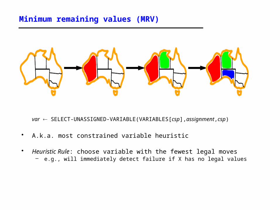
var SELECT-UNASSIGNED-VARIABLE(VARIABLES[csp],assignment,csp)
• A.k.a. most constrained variable heuristic
• Heuristic Rule: choose variable with the fewest legal moves– e.g., will immediately detect failure if X has no legal values
Degree heuristic for the initial variable
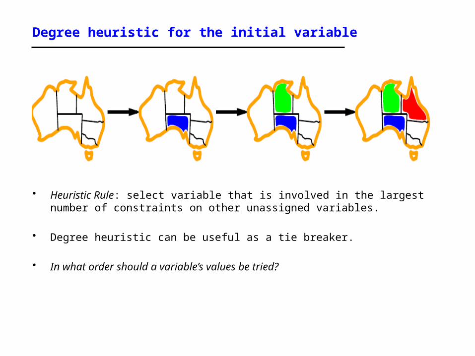
• Heuristic Rule: select variable that is involved in the largest number of constraints on other unassigned variables.
• Degree heuristic can be useful as a tie breaker.
• In what order should a variable’s values be tried?

Least constraining value for value-ordering
• Least constraining value heuristic
• Heuristic Rule: given a variable choose the least constraining value– leaves the maximum flexibility for subsequent variable assignments

Forward checking
• Can we detect inevitable failure early?– And avoid it later?
• Forward checking idea: keep track of remaining legal values for unassigned variables.
• Terminate search when any variable has no legal values.

Forward checking
• Assign {WA=red}
• Effects on other variables connected by constraints to WA– NT can no longer be red– SA can no longer be red

Forward checking
• Assign {Q=green}
• Effects on other variables connected by constraints with WA– NT can no longer be green– NSW can no longer be green– SA can no longer be green
• MRV heuristic would automatically select NT or SA next

Forward checking
• If V is assigned blue
• Effects on other variables connected by constraints with WA– NSW can no longer be blue– SA is empty
• FC has detected that partial assignment is inconsistent with the constraints and backtracking can occur.

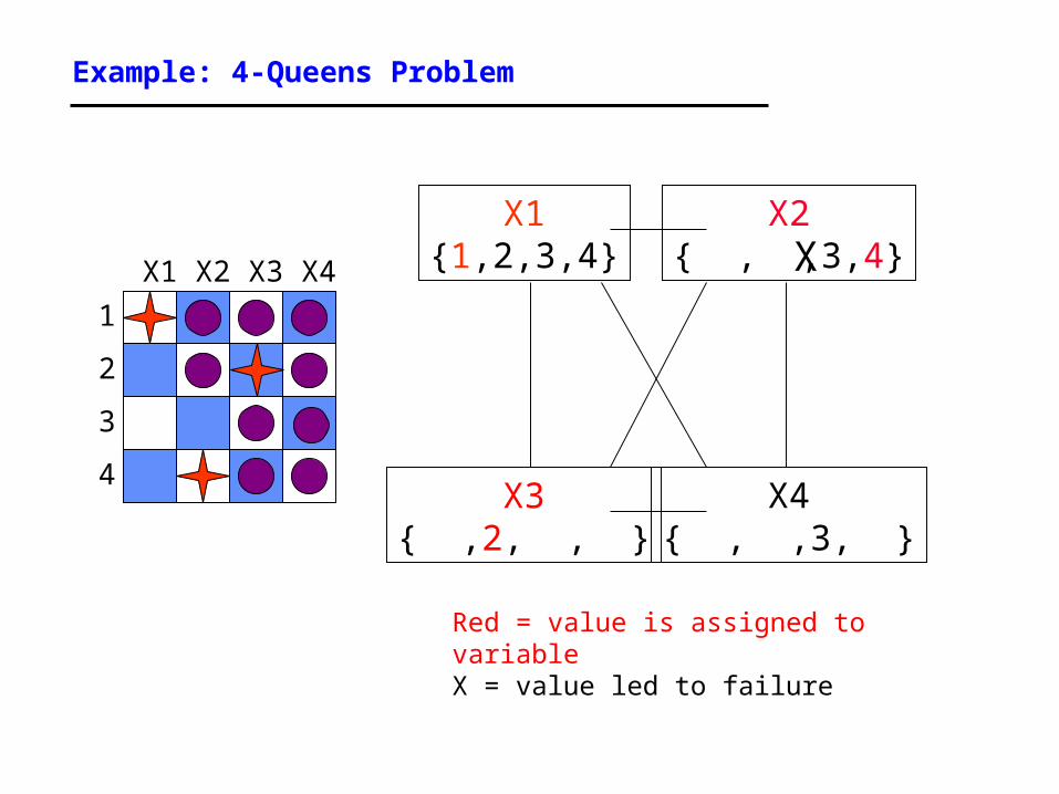
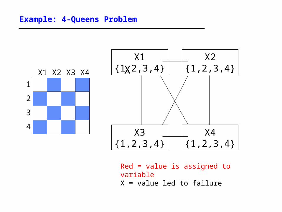
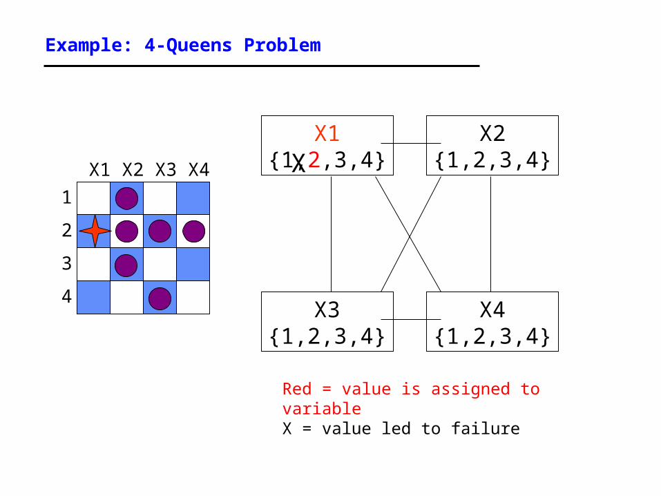
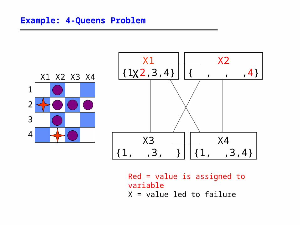
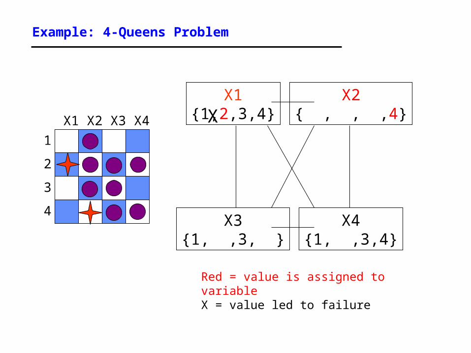
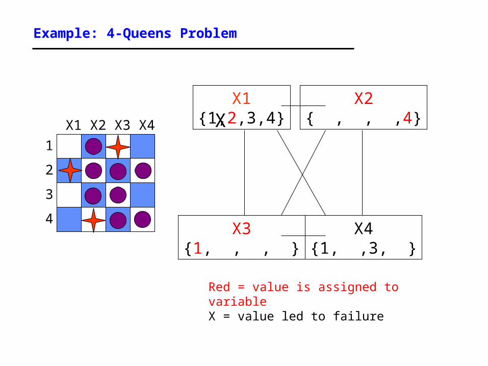
Example: 4-Queens Problem
1
3
2
4
X3X2 X4X1
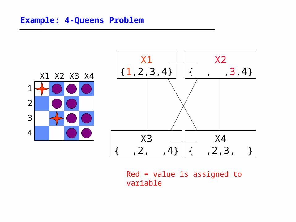
X1{1,2,3,4}
X3{1,2,3,4}
X4{1,2,3,4}
X2{1,2,3,4}

Example: 4-Queens Problem
1
3
2
4
X3X2 X4X1
X1{1,2,3,4}
X3{1,2,3,4}
X4{1,2,3,4}
X2{1,2,3,4}
Red = value is assigned to variable

Example: 4-Queens Problem
1
3
2
4
X3X2 X4X1
X1{1,2,3,4}
X3{1,2,3,4}
X4{1,2,3,4}
X2{1,2,3,4}
Red = value is assigned to variable

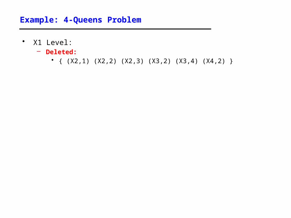
Example: 4-Queens Problem
• X1 Level:– Deleted:
• { (X2,1) (X2,2) (X3,1) (X3,3) (X4,1) (X4,4) }
• (Please note: As always in computer science, there are many different ways to implement anything. The book-keeping method shown here was chosen because it is easy to present and understand visually. It is not necessarily the most efficient way to implement the book-keeping in a computer. Your job as an algorithm designer is to think long and hard about your problem, then devise an efficient implementation.)
• One more efficient equivalent possible alternative (of many):– Deleted:
• { (X2:1,2) (X3:1,3) (X4:1,4) }

Example: 4-Queens Problem
1
3
2
4
X3X2 X4X1
X1{1,2,3,4}
X3{ ,2, ,4}
X4{ ,2,3, }
X2{ , ,3,4}
Red = value is assigned to variable

Example: 4-Queens Problem
1
3
2
4
X3X2 X4X1
X1{1,2,3,4}
X3{ ,2, ,4}
X4{ ,2,3, }
X2{ , ,3,4}
Red = value is assigned to variable
Example: 4-Queens Problem
1
3
2
4
X3X2 X4X1
X1{1,2,3,4}
X3{ ,2, ,4}
X4{ ,2,3, }
X2{ , ,3,4}
Red = value is assigned to variable

Example: 4-Queens Problem
• X1 Level:– Deleted:
• { (X2,1) (X2,2) (X3,1) (X3,3) (X4,1) (X4,4) }
• X2 Level:– Deleted:
• { (X3,2) (X3,4) (X4,3) }
• (Please note: Of course, we could have failed as soon as we deleted { (X3,2) (X3,4) }. There was no need to continue to delete (X4,3), because we already had established that the domain of X3 was null, and so we already knew that this branch was futile and we were going to fail anyway. The book-keeping method shown here was chosen because it is easy to present and understand visually. It is not necessarily the most efficient way to implement the book-keeping in a computer. Your job as an algorithm designer is to think long and hard about your problem, then devise an efficient implementation.)

Example: 4-Queens Problem
1
3
2
4
X3X2 X4X1
X1{1,2,3,4}
X3{ , , , }
X4{ ,2, , }
X2{ , ,3,4}
Red = value is assigned to variable

Example: 4-Queens Problem
• X1 Level:– Deleted:
• { (X2,1) (X2,2) (X3,1) (X3,3) (X4,1) (X4,4) }
• X2 Level:– FAIL at X2=3.– Restore:
• { (X3,2) (X3,4) (X4,3) }

Example: 4-Queens Problem
1
3
2
4
X3X2 X41X
X1{1,2,3,4}
X3{ ,2, ,4}
X4{ ,2,3, }
X2{ , ,3,4}
Red = value is assigned to variableX = value led to failure
X

Example: 4-Queens Problem
1
3
2
4
X3X2 X4X1
X1{1,2,3,4}
X3{ ,2, ,4}
X4{ ,2,3, }
X2{ , ,3,4}
Red = value is assigned to variableX = value led to failure
X

Example: 4-Queens Problem
1
3
2
4
X3X2 X4X1
X1{1,2,3,4}
X3{ ,2, ,4}
X4{ ,2,3, }
X2{ , ,3,4}
Red = value is assigned to variableX = value led to failure
X

Example: 4-Queens Problem
• X1 Level:– Deleted:
• { (X2,1) (X2,2) (X3,1) (X3,3) (X4,1) (X4,4) }
• X2 Level:– Deleted:
• { (X3,4) (X4,2) }

Example: 4-Queens Problem
1
3
2
4
X3X2 X4X1
X1{1,2,3,4}
X3{ ,2, , }
X4{ , ,3, }
X2{ , ,3,4}
Red = value is assigned to variableX = value led to failure
X

Example: 4-Queens Problem
1
3
2
4
3XX2 X4X1
X1{1,2,3,4}
X3{ ,2, , }
X4{ , ,3, }
X2{ , ,3,4}
Red = value is assigned to variableX = value led to failure
X
Example: 4-Queens Problem
1
3
2
4
X3X2 X4X1
X1{1,2,3,4}
X3{ ,2, , }
X4{ , ,3, }
X2{ , ,3,4}
Red = value is assigned to variableX = value led to failure
X

Example: 4-Queens Problem
• X1 Level:– Deleted:
• { (X2,1) (X2,2) (X3,1) (X3,3) (X4,1) (X4,4) }
• X2 Level:– Deleted:
• { (X3,4) (X4,2) }
• X3 Level:– Deleted:
• { (X4,3) }

Example: 4-Queens Problem
1
3
2
4
X3X2 X4X1
X1{1,2,3,4}
X3{ ,2, , }
X4{ , , , }
X2{ , ,3,4}
Red = value is assigned to variableX = value led to failure
X

Example: 4-Queens Problem
• X1 Level:– Deleted:
• { (X2,1) (X2,2) (X3,1) (X3,3) (X4,1) (X4,4) }
• X2 Level:– Deleted:
• { (X3,4) (X4,2) }
• X3 Level:– Fail at X3=2.– Restore:
• { (X4,3) }

Example: 4-Queens Problem
1
3
2
4
X3X2 X4X1
X1{1,2,3,4}
X3{ ,2, , }
X4{ , ,3, }
X2{ , ,3,4}
Red = value is assigned to variableX = value led to failure
X
X

Example: 4-Queens Problem
• X1 Level:– Deleted:
• { (X2,1) (X2,2) (X3,1) (X3,3) (X4,1) (X4,4) }
• X2 Level:– Fail at X2=4.– Restore:
• { (X3,4) (X4,2) }

Example: 4-Queens Problem
1
3
2
4
X3X2 X4X1
X1{1,2,3,4}
X3{ ,2, ,4}
X4{ ,2,3, }
X2{ , ,3,4}
Red = value is assigned to variableX = value led to failure
XX

Example: 4-Queens Problem
• X1 Level:– Fail at X1=1.– Restore:
• { (X2,1) (X2,2) (X3,1) (X3,3) (X4,1) (X4,4) }
Example: 4-Queens Problem
1
3
2
4
X3X2 X4X1
X1{1,2,3,4}
X3{1,2,3,4}
X4{1,2,3,4}
X2{1,2,3,4}
Red = value is assigned to variableX = value led to failure
X

Example: 4-Queens Problem
1
3
2
4
X3X2 X4X1
X1{1,2,3,4}
X3{1,2,3,4}
X4{1,2,3,4}
X2{1,2,3,4}
Red = value is assigned to variableX = value led to failure
X
Example: 4-Queens Problem
1
3
2
4
X3X2 X4X1
X1{1,2,3,4}
X3{1,2,3,4}
X4{1,2,3,4}
X2{1,2,3,4}
Red = value is assigned to variableX = value led to failure
X
Example: 4-Queens Problem
• X1 Level:– Deleted:
• { (X2,1) (X2,2) (X2,3) (X3,2) (X3,4) (X4,2) }

Example: 4-Queens Problem
1
3
2
4
X3X2 X4X1
X1{1,2,3,4}
X3{1, ,3, }
X4{1, ,3,4}
X2{ , , ,4}
Red = value is assigned to variableX = value led to failure
X
Example: 4-Queens Problem
1
3
2
4
X3X2 X4X1
X1{1,2,3,4}
X3{1, ,3, }
X4{1, ,3,4}
X2{ , , ,4}
Red = value is assigned to variableX = value led to failure
X
Example: 4-Queens Problem
1
3
2
4
X3X2 X4X1
X1{1,2,3,4}
X3{1, ,3, }
X4{1, ,3,4}
X2{ , , ,4}
Red = value is assigned to variableX = value led to failure
X

Example: 4-Queens Problem
• X1 Level:– Deleted:
• { (X2,1) (X2,2) (X2,3) (X3,2) (X3,4) (X4,2) }
• X2 Level:– Deleted:
• { (X3,3) (X4,4) }

Example: 4-Queens Problem
1
3
2
4
X3X2 X4X1
X1{1,2,3,4}
X3{1, , , }
X4{1, ,3, }
X2{ , , ,4}
Red = value is assigned to variableX = value led to failure
X
Example: 4-Queens Problem
1
3
2
4
X3X2 X4X1
X1{1,2,3,4}
X3{1, , , }
X4{1, ,3, }
X2{ , , ,4}
Red = value is assigned to variableX = value led to failure
X

Example: 4-Queens Problem
1
3
2
4
X3X2 X4X1
X1{1,2,3,4}
X3{1, , , }
X4{1, ,3, }
X2{ , , ,4}
Red = value is assigned to variableX = value led to failure
X

Example: 4-Queens Problem
• X1 Level:– Deleted:
• { (X2,1) (X2,2) (X2,3) (X3,2) (X3,4) (X4,2) }
• X2 Level:– Deleted:
• { (X3,3) (X4,4) }
• X3 Level:– Deleted:
• { (X4,1) }

Example: 4-Queens Problem
1
3
2
4
X3X2 X4X1
X1{1,2,3,4}
X3{1, , , }
X4{ , ,3, }
X2{ , , ,4}
Red = value is assigned to variableX = value led to failure
X

Example: 4-Queens Problem
1
3
2
4
X3X2 X4X1
X1{1,2,3,4}
X3{1, , , }
X4{ , ,3, }
X2{ , , ,4}
Red = value is assigned to variableX = value led to failure
X

Comparison of CSP algorithms on different problems
Median number of consistency checks over 5 runs to solve problem
Parentheses -> no solution found
USA: 4 coloringn-queens: n = 2 to 50Zebra: see exercise 5.13

Constraint propagation
• Solving CSPs with combination of heuristics plus forward checking is more efficient than either approach alone
• FC checking does not detect all failures.– E.g., NT and SA cannot be blue
Constraint propagation
• Techniques like CP and FC are in effect eliminating parts of the search space– Somewhat complementary to search
• Constraint propagation goes further than FC by repeatedly enforcing constraints locally– Needs to be faster than actually searching to be effective
• Arc-consistency (AC) is a systematic procedure for constraint propagation

Arc consistency
• An Arc X Y is consistent iffor every value x of X there is some value y consistent with x
(note that this is a directed property)
• Consider state of search after WA and Q are assigned:
SA NSW is consistent ifSA=blue and NSW=red

Arc consistency
• X Y is consistent iffor every value x of X there is some value y consistent with x
• NSW SA is consistent ifNSW=red and SA=blueNSW=blue and SA=???
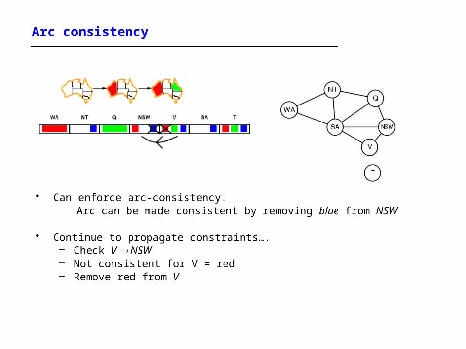
Arc consistency
• Can enforce arc-consistency:Arc can be made consistent by removing blue from NSW
• Continue to propagate constraints….– Check V NSW– Not consistent for V = red – Remove red from V

Arc consistency
• Continue to propagate constraints….
• SA NT is not consistent– and cannot be made consistent
• Arc consistency detects failure earlier than FC

Arc consistency checking
• Can be run as a preprocessor or after each assignment – Or as preprocessing before search starts
• AC must be run repeatedly until no inconsistency remains
• Trade-off– Requires some overhead to do, but generally more effective than
direct search– In effect it can eliminate large (inconsistent) parts of the state
space more effectively than search can
• Need a systematic method for arc-checking – If X loses a value, neighbors of X need to be rechecked:
i.e. incoming arcs can become inconsistent again (outgoing arcs will stay consistent).

Arc consistency algorithm (AC-3)
function AC-3(csp) returns false if inconsistency found, else true, may reduce csp domainsinputs: csp, a binary CSP with variables {X1, X2, …, Xn}
local variables: queue, a queue of arcs, initially all the arcs in csp/* initial queue must contain both (Xi, Xj) and (Xj, Xi) */
while queue is not empty do(Xi, Xj) REMOVE-FIRST(queue)
if REMOVE-INCONSISTENT-VALUES(Xi, Xj) then
if size of Di = 0 then return false
for each Xk in NEIGHBORS[Xi] − {Xj} do
add (Xk, Xi) to queue if not already there
return true
function REMOVE-INCONSISTENT-VALUES(Xi, Xj) returns true iff we delete a
value from the domain of Xi
removed falsefor each x in DOMAIN[Xi] do
if no value y in DOMAIN[Xj] allows (x,y) to satisfy the constraints
between Xi and Xj
then delete x from DOMAIN[Xi]; removed true
return removed
(from Mackworth, 1977)

Complexity of AC-3
• A binary CSP has at most n2 arcs
• Each arc can be inserted in the queue d times (worst case)– (X, Y): only d values of X to delete
• Consistency of an arc can be checked in O(d2) time
• Complexity is O(n2 d3)
• Although substantially more expensive than Forward Checking, Arc Consistency is usually worthwhile.
K-consistency
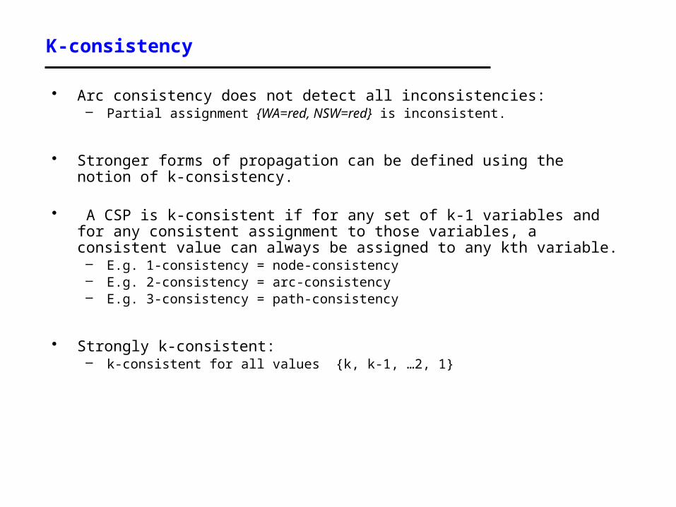
• Arc consistency does not detect all inconsistencies:– Partial assignment {WA=red, NSW=red} is inconsistent.
• Stronger forms of propagation can be defined using the notion of k-consistency.
• A CSP is k-consistent if for any set of k-1 variables and for any consistent assignment to those variables, a consistent value can always be assigned to any kth variable.– E.g. 1-consistency = node-consistency– E.g. 2-consistency = arc-consistency– E.g. 3-consistency = path-consistency
• Strongly k-consistent: – k-consistent for all values {k, k-1, …2, 1}

Trade-offs
• Running stronger consistency checks…– Takes more time– But will reduce branching factor and detect more inconsistent
partial assignments
– No “free lunch” • In worst case n-consistency takes exponential time
• Generally helpful to enforce 2-Consistency (Arc Consistency)
• Sometimes helpful to enforce 3-Consistency
• Higher levels may take more time to enforce than they save.

Further improvements
• Checking special constraints– Checking Alldif(…) constraint
• E.g. {WA=red, NSW=red}– Checking Atmost(…) constraint
• Bounds propagation for larger value domains
• Intelligent backtracking– Standard form is chronological backtracking i.e. try different value for
preceding variable.– More intelligent, backtrack to conflict set.
• Set of variables that caused the failure or set of previously assigned variables that are connected to X by constraints.
• Backjumping moves back to most recent element of the conflict set.• Forward checking can be used to determine conflict set.

Local search for CSPs
• Use complete-state representation– Initial state = all variables assigned values– Successor states = change 1 (or more) values
• For CSPs– allow states with unsatisfied constraints (unlike backtracking)– operators reassign variable values– hill-climbing with n-queens is an example
• Variable selection: randomly select any conflicted variable
• Value selection: min-conflicts heuristic– Select new value that results in a minimum number of conflicts with the
other variables

Local search for CSP
function MIN-CONFLICTS(csp, max_steps) return solution or failureinputs: csp, a constraint satisfaction problem
max_steps, the number of steps allowed before giving up
current an initial complete assignment for cspfor i = 1 to max_steps do
if current is a solution for csp then return currentvar a randomly chosen, conflicted variable from VARIABLES[csp]value the value v for var that minimize CONFLICTS(var,v,current,csp)set var = value in current
return failure

Min-conflicts example 1
Use of min-conflicts heuristic in hill-climbing.
h=5 h=3 h=1
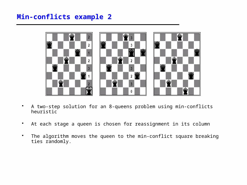
Min-conflicts example 2
• A two-step solution for an 8-queens problem using min-conflicts heuristic
• At each stage a queen is chosen for reassignment in its column
• The algorithm moves the queen to the min-conflict square breaking ties randomly.

Comparison of CSP algorithms on different problems
Median number of consistency checks over 5 runs to solve problem
Parentheses -> no solution found
USA: 4 coloringn-queens: n = 2 to 50Zebra: see exercise 6.7 (3rd ed.); exercise 5.13 (2nd ed.)

Advantages of local search
• Local search can be particularly useful in an online setting– Airline schedule example
• E.g., mechanical problems require than 1 plane is taken out of service• Can locally search for another “close” solution in state-space• Much better (and faster) in practice than finding an entirely new
schedule
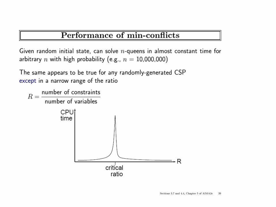
• The runtime of min-conflicts is roughly independent of problem size.– Can solve the millions-queen problem in roughly 50 steps.
– Why?• n-queens is easy for local search because of the relatively high
density of solutions in state-space
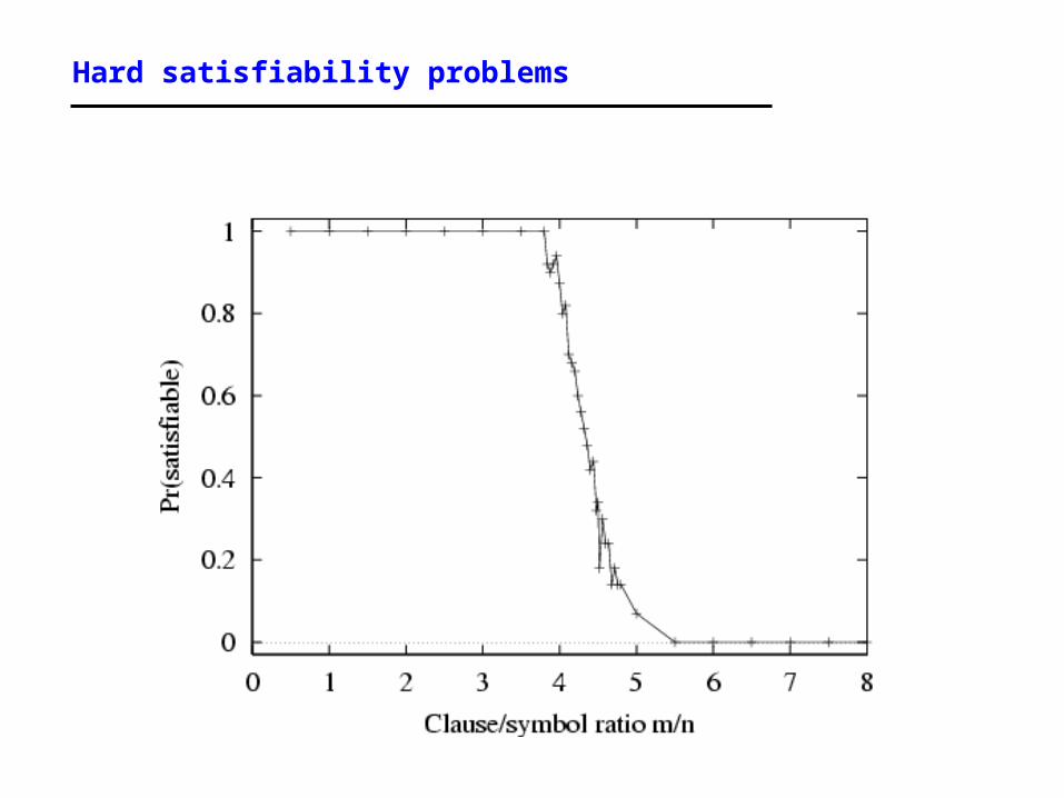
Hard satisfiability problems

Hard satisfiability problems
• Median runtime for 100 satisfiable random 3-CNF sentences, n = 50

Sudoku — Backtracking Search + Forward Checking
• R = [number of cells]/[number of filled cells]• Success Rate = P(random puzzle is solvable)• [number of cells] = 81• [number of filled cells] = variable
0.00 0.05 0.10 0.15 0.20 0.25 0.30 0.35 0.400
1000
2000
3000
4000
Avg Time vs. R
Avg Time
0.00 0.05 0.10 0.15 0.20 0.25 0.30 0.35 0.40 0.45 0.500.000.200.400.600.801.00
Success Rate vs. R
Success Rate
R = [number of cells]/[number of filled cells]
R = [number of cells]/[number of filled cells]
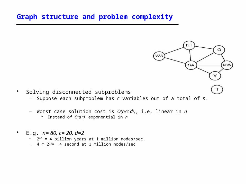
Graph structure and problem complexity
• Solving disconnected subproblems– Suppose each subproblem has c variables out of a total of n.
– Worst case solution cost is O(n/c dc), i.e. linear in n• Instead of O(d n), exponential in n
• E.g. n= 80, c= 20, d=2– 280 = 4 billion years at 1 million nodes/sec.– 4 * 220= .4 second at 1 million nodes/sec

Tree-structured CSPs
• Theorem: – if a constraint graph has no loops then the CSP can be solved
in O(nd 2) time– linear in the number of variables!
• Compare difference with general CSP, where worst case is O(d n)

Summary
• CSPs – special kind of problem: states defined by values of a fixed set of variables,
goal test defined by constraints on variable values
• Backtracking=depth-first search with one variable assigned per node
• Heuristics– Variable ordering and value selection heuristics help significantly
• Constraint propagation does additional work to constrain values and detect inconsistencies– Works effectively when combined with heuristics
• Iterative min-conflicts is often effective in practice.
• Graph structure of CSPs determines problem complexity– e.g., tree structured CSPs can be solved in linear time.