IEEE TRANSACTIONS ON INSTRUMENTATION AND MEASUREMENT, VOL. 45, NO. 3, JUNE 1996 715

Considering Clock Errors in Numerical Simulations

Alexander Harting

Abstract-The description of a dynamic system often involves a wide range of time intervals. Before considering clock errors in numerical simulations of such systems, it is found necessary to simulate the clock itself over the full scale of times involved. A scheme is presented to do such a clock simulation numerically and to prepare the result as an input for the simulation of the dynamic system. Some interesting consequences are discussed together with two numerical examples.

I. MOTIVATION

HE last few decades saw a tremendous improvement in T the performance of clocks. Today, intervals of time can be measured, time scales can be kept, and clocks can be syn- chronized globally with a precision that is hardly observable in everyday life. Still, in disciplines such as astronomy, geodesy and navigation, measurement techniques exploit the available timing accuracy to the utmost, and the practical demand for increasing clock performance is not at an end.

Dynamic time, which is the independent variable in equa- tions of motion, is uniform to the degree which we can trust the underlying theory. Measurements, on the other hand, are timed with clocks that do not tell perfectly uniform time. Evaluating such measurements in dynamic calculations of physical systems, one is frequently confronted with the need to analyze certain influences by simulation.

The present paper was motivated by a study of the influence of various clocks’ performance on the navigational precision of the satellite tracking system PRARE [l]. Whereas some examples in the following discussions will be taken from spacecraft flight dynamics, the material presented is on the numerical simulation of clock errors in general and may be useful for a variety of applications.

Let us imagine a low earth-orbiting satellite with a tracking system that measures distances to a set of ground transponders depending on its on-board clock. Then, various time intervals are involved: an individual range measurement takes some- thing like 10 ms; measurements may be done consecutively once per second during the ten to fifteen minutes visibility of a ground station; there are contacts with the same ground station every couple of hours, and the evaluation of the tracking data will be done over an arc length of several days. Timing accuracy affects both the measured quantity itself, which is a

Manuscript received November 15, 1994; revised August 28, 1995. This work was supported in part by the European Space Agency ESA.

The author was with GeoForschungsZentrum Potsdam (GFZ), D-82230 Oberpfaffenhofen, Germany. He is now with Oldenburg Polytechnic, D-26926 Elsfleth, Germany.

Publisher Item Identifier S 0018-9456(96)03088-4.

travel time, and the time tag, which says to what instant on a global time scale the value is referred.

The stability, which characterizes a clock, is assumed to be given as a function of the measured time interval in a way that will be discussed in more detail below. Now, if we could assign a random uncertainty in measuring any time interval, we still do not know how to simulate the above scenario, because an independent attachment of errors to the occurring time intervals would violate important correlations. This is obvious, because the same clock reading may serve as the beginning mark of a travel time measurement, the distinction of a single measurement within a block and the large-scale time tag of an entire block. A correct description of clock errors must superimpose the characteristics over all time intervals. Simulating a random error in a 10 ms interval and, independently, another error in the next 10 ms interval, one is certainly wrong to ignore the momentary state of the clock error on a larger time scale. Therefore, to consider clock errors correctly in such simulations it is necessary to explicitly imitate the clock over the full period of interest with a resolution better than the smallest time interval involved.

In the following, we shall analyze the properties of a clock given by its stability function and present a technique to imitate the clock such that use of the generated clock error as an input for subsequent simulations is straightforward and clear. Using numerical examples, the results and their consequences will be discussed.

11. CHARACTERIZATION OF CLOCK ERRORS

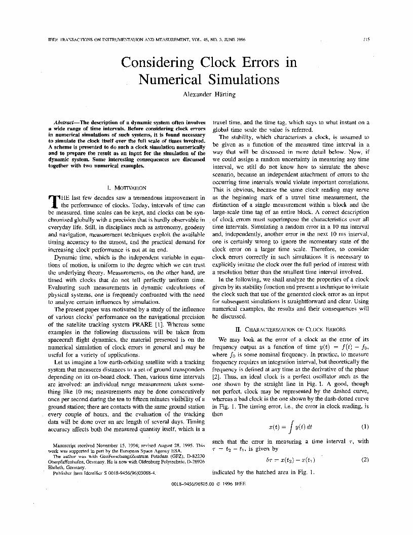
We may look at the error of a clock as the error of its frequency output as a function of time y(t) = f ( t ) - f o , where f o is some nominal frequency. In practice, to measure frequency requires an integration interval, but theoretically the frequency is defined at any time as the derivative of the phase [ 2 ] . Thus, an ideal clock is a perfect oscillator such as the one shown by the straight line in Fig. 1. A good, though not perfect, clock may be represented by the dashed curve, whereas a bad clock is the one shown by the dash-dotted curve in Fig. 1. The timing error, i.e., the error in clock reading, is then

such that the error in measuring a time interval r , with r = t 2 - t l , is given by

(2) ST = Z ( t 2 ) - z(t1)

indicated by the hatched area in Fig. 1.

0018-9456/96$05.00 0 1996 IEEE

716 IEEE TRANSACTIONS ON INSTRUMENTATION AND MEASUREMENT, VOL. 45, NO. 3, JUNE 1996

~

11 t2 t

Fig. 1. Definition of quantities associated with clock errors.

We may now introduce the relative frequency error, aver- aged over the integration time T as

The prescription is to measure T with the same clock many times consecutively without a dead time in between. In the limit of large N the expression

(4)

is known as the Allan variance [3] , which is universally accepted as a measure of clock performance. Please note that this is not the deviation from a mean value, but the average deviation between nearest neighbor intervals. Also, it is obvious that a constant frequency offset will not affect a , ( ~ ) , i.e., the zero point on the y(t)-scale is, in fact, arbitrary.

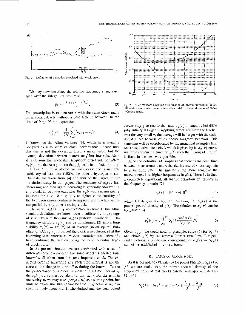
In Fig. 2 ay(.) is plotted for two clocks: one is an ultra- stable crystal oscillator (USO), the other a hydrogen maser. The data are taken from [4] and will be the target of our simulation study in this paper. The tendency of ay(7) first decreasing and then again increasing is generally observed in any clock. In our two examples the a,(T)-curves are nearly identical for T < lo-' s; only at higher T the stability of the hydrogen maser continues to improve and reaches values unequalled by any other existing clock.

The curve ay(.) fully characterizes a clock. If the Allan standard deviations are known over a sufficiently large range of T , clocks with the same a , ( ~ ) perform equally well. The frequency stability o,(T) can be transformed [2] into a time stability a , ( ~ ) = TO,(.) or an average (mean square) time offset of J27a,(r), provided the clock is synchronized at the beginning of the interval 7. Previous numerical simulations [ 5 ] have confirmed the relation for O, for some individual types of clock noise.

In the present situation we are confronted with a set of different, some overlapping and some widely separated time intervals, all taken from the same imperfect clock. The ex- pected error in measuring any such time interval is not the same as the change in time offset during the interval. To see the performance of a clock in measuring a time interval TO

the a,(~)-curve must be taken not only at TO. For the error in measuring TO we may take J ~ T ~ ~ , ( T o ) as a starting point, but must be aware that this cannot be true in general as we can see intuitively from Fig. 1. The dashed and the dash-dotted

............... .................... ................... ; ................... j ................... j .................... ; ; ; ................ f ................

^ ............................. .: .............. ...,: .................. r. .................. ~ .................... ~ .................. i q I:,:::::::::::.::;:::..?.. . c ' - ' s ; ........... i.. ................. i ........................................ i .................... ;... ............. . .

+J

i 1 ............. ................. i ............ 5 ...... : .................... .................... ................... ................. .: ................. .; ~. -I .................. i ................... i ................................................. .................... ................... i:! ................

tau I sec

Fig. 2. M a n standard deviation as a function of integration interval for two different clocks: dashed curve: ultrastable crystal oscillator, dash-dotted curve: hydrogen maser.

curves may give rise to the same a , ( ~ ) at small 7 , but differ substantially at larger T . Applying errors similar to the hatched area for very small 7 , the average will be larger with the dash- dotted curve because of its poorer longterm behavior. This statement will be corroborated by the numerical examples later on. Thus, to simulate a clock which is given by its a,(T)-curve, we must construct a function p ( t ) such that, using (4), ay(.) is fitted in the best way possible.

Since the definition (4) implies that there is no dead time between measurement intervals, the inverse of T corresponds to a sampling rate. The smaller T the more sensitive the measurement is to higher frequencies in p ( t ) . There is, in fact, a completely equivalent, alternative definition of stability in the frequency domain [2]

where FT denotes the Fourier transform, i.e., S,(f) is the power spectral density of y(t). The relation to a , ( ~ ) can be formulated as

Given a, (7) we could now, in principle, solve (6) for S, ( f ) and obtain y(t) by the reverse Fourier transform. For gen- eral functions, a one-to-one correspondence a , ( ~ ) t-f S,(f) cannot be established in closed form.

111. TYPES OF CLOCK NOISE

As it is possible to evaluate (6) for power functions S, (f) oc f" we are lucky that the power spectral density of the frequency noise of real clocks can be well approximated by 121, [41

HARTING: CONSIDERING CLOCK ERRORS IN NUMERICAL SIMULATIONS 7 17

TABLE I TYPES OF CLOCK NOISE WKH THEIR CONTRBUTIONS

TO SPECTRAL D E N S ~ Y AND ALLAN VARIANCE

TABLE I1

NOISE IN SIMULATIONS WITH RANDOM NUMBERS PRINCIPLE OF GENERATING VARIOUS TYPES OF

S,(f) CTy2@) type of noise

h2p (b,3fJ/(47?T2) white phase

h,f h,[6+31n(21if,z)-ln21/(4~~) flicker phase

h, W(W white frequency hJf h.,2ln2 flicker frequency

h-@ h.,(47?/6)~ random walk frequency

type of noise frequency error algorithm

white phase y,=rand,-ranc$, white frequency YFand,

random walk frequency yi=yi.l+ran4

In this equation each term can be identified with an individual type of noise, and the relation to cy(.) is summarized in Table I.

With the expressions S, (f) representing white phase noise and flicker phase noise the integral in (6) does not exist. In these cases the high-frequency cutoff fh has been introduced to replace the upper integration limit. This technical measure can be physically justified. The corresponding cy (T)-curves would indeed diverge as T + 0. It means that there is increasing noise “power” the higher the frequency comes or, in other words, the closer we are looking at y( t ) . In our simulations we are free to chose fh at any frequency (e.g., fh = 1000 Hz) that is higher than the largest occurring 7-l. Practically we may regard the high-frequency cutoff as the upper limit in the spectral bandwidth of our experimental apparatus.

It is instructive to identify the types of noise of real clocks’ cy(T)-curves as in Fig. 2. At small T the Allan standard deviations of both clocks behave as 1 / ~ , corresponding to white phase noise. From about 10-’ s the crystal oscillator is dominated by a pronounced floor of flicker frequency noise, which, from about lo2 s, is taken over by frequency random walk. In the case of the H-maser the transition to flicker noise is smooth and slow, reaching the minimum at lo4 s. The H- maser does not exhibit random walk noise. AS T -+ cc the crystal oscillator and the H-maser (and, in fact, most clocks) are dominated by a linear frequency drift, which can easily be seen to produce a gy(.) 0: T. This has not been mentioned in the previous classification because its power spectral density is zero. Also, since such a drift can be corrected by monitoring the clock, it is not considered any further for the purpose of our simulations.

Iv. GENERATION OF NOISE FROM RANDOM NUMBERS

Let us use a uniform deviate random number generator scaled to the interval [-0.5,0.5]. It is then easy to verify that a sequence of such random numbers, if combined according to Table 11, has the qualities of various types of noise.

Given an algorithm for the simulation of frequency error, the corresponding time error is easily constructed from (1). An example for white frequency noise is given in Fig. 3.

Table I1 does not mention flicker noise. Whereas flicker phase noise is unimportant in our case (as well as in many

random number

‘“0 100 200 300 400 500 600 700 800 900 loo0

Fig. 3. White frequency noise (above) simulated from random numbers with the corresponding time error (below). Arbitrary scaling, only to visualize technique.

A. Simulation of Flicker Noise

Flicker noise is not easy to simulate. The reason is rooted in the fact that the power spectral density (see (7)) goes with an odd integer. Details can be found in [6]. Adapted from the same reference, the algorithm

yn = 7 ~ - ~ / ~ r a n d l + (n - 1)-2/3rand2 + . . . + rand, (8)

has been found to produce good results. Note that, to calculate the nth flicker number, all previous

n - 1 random numbers must be added up again with different coefficients. This makes it exceedingly expensive if many flicker numbers are needed. Computationally, the effort is tolerable for n up to a few thousand.

Modifications of (8) (such as increasing the negative power of n for the “older” terms with a cutoff in the number of terms to be dragged along) have been tried in order to get easier access to more flicker numbers. None of these modifications produced a satisfactory result. It was therefore decided to do simulations with (8) as it is.

v. APPROACH FOR SIMULATING THE CLOCK ERRORS

others), we need flicker frequency noise to properly describe the given ~ ~ ( ~ ) - c u r v e s .

Let us set out to provide the time error z( t ) for 7 days in 1 ms steps as direct access files. Of course, the design of z ( t )

718 IEEE TRANSACTIONS ON INSTRUMENTATION AND MEASUREMENT, VOL. 45, NO. 3, JUNE 1996

must be adapted to the specific case to be simulated. In the present situation, 7 days are necessary because the equations of motion will have to be integrated over that period. To be on the safe side, a resolution of 1 ms has been chosen as one order of magnitude below the smallest measured time interval. Storage in direct access files is convenient, eliminating the need in the application program to read z ( t ) into huge arrays.

It is not possible to carry out this scheme in a fully consistent way for two reasons: first, the complete file would consist of 6 x lo8 records and, even worse, the description of the US0 would need approximately lo7 flicker numbers. Instead, we shall produce one file over the full period with a larger step size and another file for the period between the large steps in 1 ms steps and use the second file to “interpolate”. Since the second file repeats between each of the records of the first file, a correlation is introduced, rendering the model imperfect. This correlation, however, seems to be tolerable as we shall see below.

A. Generation of Error Function for U S 0

6048 steps of 100 s. It is generated as The large-step file contains only frequency random walk in

yi = y;-1 + 2.0(10-14)(rand) z; = zi-1 + lOO(y;).

The small-step file contains white phase noise and flicker frequency noise in lo5 steps of 1 ms. It is generated as

yz = yf + 1.2(10-10)(rand-rand,,,,) if (z = 20 . integer) then

yz = 2.5( 10-12)(next flicker number)

Yf = Ya

end if

2, = IC,-~ + 1 0 - ~ ( ~ , )

B. Generation of Error Function for H-Maser

noise in 604800 steps of 1 S. It is generated as The large-step file contains white noise and flicker frequency

ya = yfw + l.2(10~10)(rand-rand,,,,) if (z = 4 . integer) then

ya = yff + 6.0(10-11)(rand)

Yfw = Ya

end if if (z = 5000 . integer) then

yz = 5.0(10-12)(next flicker number)

Yff = Yz

Yfw = Yz

end if 2, = zaP1 + 1 0 - ~ ( ~ , ) .

1 ..................... ...... .....; ................... i ................................... .; ................. ; ............... /- ...........

: - I .................. + ............ j... .......... ..j ........... ..................................... 4 ....................................... .................. ................. .................... .................... .................... ................... ....................

.............................. .............................................................. .. . . .

- ” ..; ; / :

._

10-13 - 10-2 10-1 100 101 102 103 104 105 io6

tau / sec

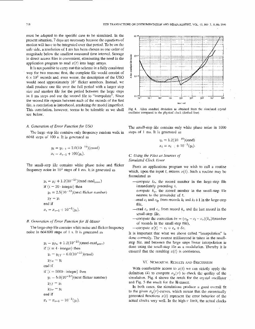
Fig. 4. oscillator compared to the physical clock (dashed line).

Allan standard deviation as obtained from the simulated crystal

The small-step file contains only white phase noise in 1000 steps of 1 ms. It is generated as

ya = 1.2(10-1°)(rand) 2a = zz-l + 1 0 - ~ ( ~ , ) .

C. Using the Files as Sources of Simulated Clock Error

From an applications program we wish to call a routine which, upon the input t , retums z( t ) . Such a routine may be formulated as

--compute 51, the record number in the large-step file

--compute IC,, the record number in the small-step file

-read el and elp from records kl and kl + 1 in the large-step

-read e, and e, from record IC, and the last record in the

--compute the correction Se = (elp - el - e,)(k,)/(number

--compute x ( t ) = el + e, + 6e.

immediately preceding t ,

nearest to the remainder of t ,

file,

small-step file,

of records in the small-step file),

It is important that what we above called “interpolation” is done correctly. The nearest millisecond is taken in the small- step file, and between the large steps linear interpolation is done using the small-step file as a modulation. Thereby it is ensured that the resulting z( t ) is continuous.

VI. NUMERICAL RESULTS AND DISCUSSION

With comfortable access to z ( t ) we can strictly apply the definition (4) to compute cy(.) to check the quality of the simulation. Fig. 4 shows the result for the crystal oscillator and Fig. 5 the result for the H-maser.

In both cases, the simulations produce a good overall fit to the given cy(7)-curves, which means that the numerically generated functions z ( t ) represent the error behavior of the actual clocks very well. In the high-7- limit, the actual clocks

HARTING: CONSIDERING CLOCK ERRORS IN NUMERICAL SIMULATIONS 719

................ ...... ........ ...................................... i .................... .................. i ................. .i .................

- : 4 t .............. ................... ; ..... e ..... ; .................... i.* ................. 1 ................. i .......................................

1 0 ' 5

.................. + ................. + ....................................... .: .................... 2 ................ ...+ .................... ! .................. 10-16

10-3 10-2 10-1 io0 101 102 103 104 10s

tau / sec tau I sec

Fig. 5. Allan standard deviation as obtained from the simulated H-maser compared to the physical clock (dash-dotted line).

Fig. 6. solid curve: result of simulation, dashed curve: J2 . u ~ ( T ) . T.

Average error in measuring time intervals T with the US0 clock;

tend toward a linear behavior, whereas the simulated US0 10~9 and H-maser go as JT and as a constant respectively. As

mentioned above the linear frequency drift was not included in the 4mulations even though it could have been done easily. 10 ' 0

The ay(^) of the simulated crystal oscillator exhibits a kind of step just below T = 10' s. This is an actual property of the simulated .r(f), and it is not a discontinuity. In this case the bridging between the small-step tile and the large-step file, which occurs at T = lo2 s, is not perfect, because thc small- step f i le introduces only a weak modulation on top of the large-step random walk.

In general, however, we have produced a good and useful description of the clocks over the required rangc of time intervals. For applications programs it is considered a great advantage that the simulated T ( ! ) can be taken directly as 1 0 3 102 I O I 100 IO' 102 IO' 1 0 4 105

an erroneous clock reading. The quality of s ( t ) is checked outside, and there is no need for interpreting the clock error representation inside the application.

$ l o "

$ 2

I o I'

wu 1 sec

Fig. 7. Average error in measuring time Interval\ T with thc ti-mawr, \ohd cline: r c d t of \imulation, da\hed curve: J2 u ~ ( T ) . T

A. Time Interval Measurement Error As a simple application we can compute the average error

in measuring time intervals withi a clock in the sense of our discussion in Section I1 above. This is done by applying (2) many times statistically over a wide range of the simulated functions ~ ( t ) . In Fig. 6 (USOl) and Fig. 7 (H-maser) the results are shown in relation to the lengths of the measured time intervals and compared with ,/2aY(7) . T , which is often used as an estimate.

It becomes apparent that ,/:2ay(~) . T is only a rough approximation. In some cases (HLmaser at small T ) the actual error is smaller, in other cases (in particular US0 near T = 1 s) the actual error is up to 10 times larger than J2aY(7) . T .

Also, at very small T (lo-' s) the average error of the US0 is about twice as large as that of the H-maser even though, there, the ay are the same. Roughly speaking, with white noise and flicker noise being dominant, the actual error tends to be overestimated by J2aY(7) . T . The presence of random walk, which is quite pronounced in our US0 example, leads to an underestimate. As it was discussed with Fig. 1 the average

error in measuring small intervals also reflects the longer-term behavior. The results of the simulations substantiate this very clearly.

VII. CONCLUSION

To investigate the influence of clock error in numerical simulations of dynamic systems, it is found necessary to imitate the clock, which is supposed to be given by its Allan standard deviation a , ( ~ ) , over the entire period of interest. A simulation scheme has been developed and was proven with two numerical examples. Mainly because of the difficulty to generate flicker noise it was necessary to distinguish between short-term and long-term behavior. The clock error functions fit the two examples very well and render it promising that any clock error can be simulated with an adapted scheme.

In all cases the entire ay(T)-curve must be taken into account, even when looking only at a single time interval. For the average error in measuring a time interval TO, the expression ,/2 . aY(7o) . TO is only a rough approximation.

720 IEEE TRANSACTIONS ON INSTRUMENTATION AND MEASUREMENT, VOL. 45, NO. 3, JUNE 1996

The result of the presented clock error representation is an error function s(t), which can be incorporated into numerical simulations of dynamic systems without any uncertainty in the meaning.

ACKNOWLEDGMENT The author is grateful for many fruitful, stimulating and

enjoyable discussions with H. Meixner, F. Flechtner, F.-H. Massmann and C. Reigber.

REFERENCES

[ l ] P. Hart1 and C. Reigber, Die Geowissenschaften, vol. 9, p. 156, 1991. [2] J. A. Barnes etal., IEEE Trans. Instrum. Meas., vol. IM-20, p. 105, 1971. [3] D. W. Allan, in Proc. IEEE, 1966, vol. 54, p. 221. [4] G. Busca, “H-maser frequency standards: Their performance and their

uses,” 1st Working Meeting on Hydrogen Maser Clocks in Space, ESA, Paris, 1993, unpublished.

[5] P. Kartaschoff, IEEE Trans. Instrum. Meas., vol. IM-28, p. 193, 1979. [6] J. A. Barnes and D. W. Allan, Proc. IEEE, vol. 54, p. 176, 1966. [7] C. Audoin and P. Lesage, IEEE Trans. Instrum. Meas., vol. IM-22, p.

157, 1973.

geodetic purposes. He PRARE master station navigation and physics,

Alexander Harting received the degree in physics in 1981, and the doctor’s degree in 1984 from the University of Regensburg, Germany.

From 1984 to 1992, he was with Satellite Operational Services GmbH, responsible for projects in the field of space flight dynamics. From 1993 to 1995, he was a research scientist at GeoForschungsZentrum Potsdam (GFZ), where he was involved in the acquisition and processing of data from the Precise Range and Range Rate Equipment (PRARE), a satellite payload for

developed software for the reference clock at the . Since 1995, he has been a professor for technical Oldenburg Polytechnic, Elsfleth, Germany.