connecting antarctic cross-slope exchange with southern ocean overturning

Connecting Antarctic Cross-Slope Exchange with Southern Ocean Overturning

ANDREW L. STEWART AND ANDREW F. THOMPSON

Environmental Sciences and Engineering, California Institute of Technology, Pasadena, California

(Manuscript received 14 October 2012, in final form 11 March 2013)

ABSTRACT

Previous idealized investigations of Southern Ocean overturning have omitted its connection with the

Antarctic continental shelves, leaving the influence of shelf processes on Antarctic Bottom Water (AABW)

export unconsidered. In particular, the contribution of mesoscale eddies to setting the stratification and

overturning circulation in the Antarctic Circumpolar Current (ACC) is well established, yet their role in

cross-shelf exchange of water masses remains unclear. This study proposes a residual-mean theory that

elucidates the connection between Antarctic cross-shelf exchange and overturning in the ACC, and the

contribution of mesoscale eddies to the export of AABW. The authors motivate and verify this theory using

an eddy-resolving process model of a sector of the SouthernOcean. The strength and pattern of the simulated

overturning circulation strongly resemble those of the real ocean and are closely captured by the residual-

mean theory. Over the continental slope baroclinic instability is suppressed, and so transport by mesoscale

eddies is reduced. This suppression of the eddy fluxes also gives rise to the steep ‘‘V’’-shaped isopycnals that

characterize the Antarctic Slope Front in AABW-forming regions of the continental shelf. Furthermore, to

produce water on the continental shelf that is dense enough to sink to the deep ocean, the deep overturning

cell must be at least comparable in strength to wind-driven mean overturning on the continental slope. This

results in a strong sensitivity of the deep overturning strength to changes in the polar easterly winds.

1. Introduction

The meridional overturning circulation (MOC) de-

scribes the global-scale meridional transport of ocean

water masses (Talley et al. 2003). It exerts a substantial

influence over climate via interhemispheric transport of

heat and salt, in addition to biogeochemical tracers such

as oxygen and carbon (Kuhlbrodt et al. 2007; Lynch-

Stieglitz et al. 2007). This article focuses on the Southern

Ocean, which has been identified as a region of partic-

ular dynamical and climatic importance for the MOC

(Marshall and Speer 2012). Here strong, midlatitude

westerly winds produce an isopycnal tilt that allows deep

waters to upwell to the surface. These waters are then

transported north by surface currents and subducted as

Antarctic Intermediate Water (AAIW) or transported

south toward the Antarctic continental shelf (Speer et al.

2000). In certain regions, largely confined to the Weddell

and Ross Seas, the upwelled water mixes with fresh

glacial meltwater, and high-salinity shelf water produced

by rejection of brine during sea ice formation (Gill 1973;

Orsi and Wiederwohl 2009). The resulting mixture sinks

down from the continental shelf and spreads throughout

the global ocean as Antarctic Bottom Water (AABW)

(Gordon 2009).

The export of AABWconstitutes the lowest branch of

the global MOC and is arguably the most climatically

important over millennial time scales (Marshall and

Speer 2012). AABW consists largely of waters that have

recently been in contact with the atmosphere and so

carries oxygen to the deep ocean (Orsi et al. 2001). The

deep branch of the MOC also stores dissolved CO2 and

may thereby drive millennial-scale climate change via

exchanges with the atmospheric CO2 reservoir (Russell

et al. 2006; Toggweiler et al. 2006; Toggweiler 2009;

Skinner et al. 2010).

The climatic influence of the Southern Ocean MOC

has motivated a series of studies to elucidate the rela-

tionship between surface forcing of the Antarctic Cir-

cumpolar Current (ACC) and the resultant stratification

and overturning (e.g., Hallberg and Gnanadesikan 2006;

Hogg et al. 2008). Anthropogenic CO2 emissions have

led to an intensification of the midlatitude westerlies in

Corresponding author address: Andrew L. Stewart, Environ-

mental Science and Engineering, MC 131-24, California Institute

of Technology, Pasadena, CA 91125.

E-mail: [email protected]

JULY 2013 S TEWART AND THOMPSON 1453

DOI: 10.1175/JPO-D-12-0205.1

� 2013 American Meteorological Society

the past few decades (Shindell and Schmidt 2004; Polvani

et al. 2011), characterized by a strengthening of the

southern annular mode (Thompson andWallace 2000;

Thompson et al. 2000). Meanwhile, millennial-scale CO2

exchanges between the deep ocean and the atmosphere

have also been attributed to latitudinal shifts of the

westerlies (Russell et al. 2006; Toggweiler et al. 2006;

Toggweiler 2009). This has motivated a particular focus

on the response of the MOC to changes in the mid-

latitude westerly wind strength (e.g., Hofmann and

Maqueda 2011; Meredith et al. 2011; Abernathey et al.

2011).

The upper branch of the Southern Ocean MOC may

be explained dynamically using residual-mean theory

(RMT) (Andrews et al. 1987; Plumb and Ferrari 2005;

Kuo et al. 2005). The observed overturning is described

as a relatively small residual, resulting from an imbal-

ance between a wind-driven mean overturning and a

counteracting ‘‘eddy’’ overturning (Marshall and Radko

2003; Olbers and Visbeck 2005; Marshall and Radko 2006;

Radko and Marshall 2006). RMT qualitatively explains

the observed tracer distributions in the Southern Ocean

(Karsten and Marshall 2002) and compares favorably

with idealized eddy-resolving simulations (Abernathey

et al. 2011). Wolfe and Cessi (2011) extended RMT to

model the pole-to-pole MOC, and found good agree-

ment with eddy-resolving simulations of an entire ocean

basin. Ito and Marshall (2008) applied RMT to the deep

MOC, and derived a scaling for the diapycnal mixing

rate needed to allow transport of AABW across iso-

pycnals outcropping from the ocean bed. Saenko et al.

(2011) combined an extension of this scaling with eddy-

permitting simulations of the Southern Ocean to predict

an increase in AABW export in response to strengthen-

ing of the midlatitude westerlies. Nikurashin and Vallis

(2011) developed a residual-mean model of a diffusively

driven deep overturning cell, and Nikurashin and Vallis

(2012) extended this model to include a quasi-adiabatic

upper cell originating from a northern high-latitude

convective region. Their model agreed qualitatively with

coarsely resolved simulations using parameterized eddy

transports.

The present work employs RMT as a model of both

the upper and lower overturning cells, including an

idealized Antarctic continental shelf, in concert with

idealized eddy-resolving simulations of a sector of the

Southern Ocean. This connects our theoretical under-

standing of the MOC in the ACC with that of the

Antarctic Slope Front (ASF), a weaker westward cur-

rent that flows along the continental slope around most

of Antarctica (Jacobs 1991; Muench and Gordon 1995;

Chavanne et al. 2010). The ASF is driven by circumpolar

easterly winds around the Antarctic margins (Large and

Yeager 2009), and is characterized by steep ‘‘V’’-shaped

isopycnals in AABW-forming regions of the conti-

nental shelf (Gill 1973; Thompson and Heywood 2008).

Our understanding of the dynamical processes that set

the structure of the ASF is limited to quite idealized

models. For example, Ou (2007) proposed a box-type

model of the ASF that presupposed the ‘‘V’’-shaped

isopycnal structure and then balanced heat and salt

fluxes across the continental slope. More recently Baines

(2009) constructed more sophisticated analytical solu-

tions for a two-dimensional flow that is entrained into

a turbulent down-slope bottom current. In this article, the

structure of the ASF is explained in section 5 as a con-

sequence of the eddy-mean overturning balance of RMT,

once the tendency of the continental slope to suppress

baroclinic instability is accounted for.

Connecting the overturning in the ACC with that

over the Antarctic continental shelf allows us to ana-

lyze the influence of shelf processes on the global MOC.

In particular, the contribution of mesoscale eddies to

the cross-shelf transport remains unclear, though recent

high-resolution modeling studies suggest that eddies

may dominate the shoreward transport of Circumpo-

lar Deep Water (CDW) beneath Antarctic ice shelves

(Thoma et al. 2008; Dinniman et al. 2011; Nøst et al.

2011). We will focus on the sensitivity of the MOC to

changes in the easterlies that drive the ASF. While the

midlatitude westerlies have intensified over the past

few decades (Shindell and Schmidt 2004; Polvani et al.

2011), the trend in the polar easterlies is ambiguous (Son

et al. 2010; Polvani et al. 2011), as are model predictions

for their strength at the last glacial maximum (Krinner

and Genthon 1998; Kitoh et al. 2001). Stewart and

Thompson (2012) have recently shown that the export of

AABW is much more sensitive to changes in the polar

easterlies than the midlatitude westerlies. This sensi-

tivity is explained succinctly by our RMT approach and

is explored further in section 6.

The structure of this paper is as follows. In section 2

we describe our idealized eddy-resolving numerical sim-

ulations of the ACC and ASF and diagnose the MOC

and cross-shelf heat transport. In section 3 we derive

residual-mean equations and boundary equations suit-

able for our domain. In section 4 we discuss the param-

eterizations of the isopycnal and diapycnal diffusivities

required to represent the heat transport over the Ant-

arctic continental slope and close to the ocean bed. In

section 5 we obtain approximate and numerical solutions

to the residual-mean equations. Finally, in section 6 we

examine the sensitivity of the stratification and over-

turning circulation to variations in the imposed wind

stress, and compare the results of our theory with those

of our eddy-resolving simulations.

1454 JOURNAL OF PHYS ICAL OCEANOGRAPHY VOLUME 43

2. Eddy-resolving simulations of the deepoverturning circulation

In this section we discuss the overturning circulation

and export of dense water from the continental shelf

in our reference simulation, whose imposed forcing

most strongly resembles conditions in the contempo-

rary Southern Ocean. This simulation motivates some

aspects of the residual-mean theory described in sec-

tions 3–5.

a. Modeling preliminaries

We used the Massachusetts Institute of Technology

(MIT) general circulation model (MITgcm) to con-

duct all of the simulations described herein (Marshall

et al. 1997a,b). The model parameters are summarized

in Table 1. We model a sector of the Southern Ocean

and the Antarctic continental shelf as a zonally reentrant

channel in Cartesian geometry. The channel is zonally

symmetric, and its depth is described by

h(y)5Hs 11

2(H2Hs)

�11 tanh

�y2Ys

Ws

��. (1)

This geometry is illustrated in Fig. 1. For simplicity and

computational efficiency we have used a somewhat

shallower channel than the ;4000-m depth of the real

Southern Ocean.

Flow in the channel is governed by the three-

dimensional, hydrostatic Boussinesq equations (e.g.,

Vallis 2006). We neglect the dynamical influence of sa-

linity, which is fixed at 35 psu everywhere, and prescribe

a linear dependence of density on temperature. Tem-

perature is advected using a third-order direct space–

time flux-limiting scheme. We parameterize dense water

formation by directly relaxing the temperature toward

uc 5218C over a localized area of the shelf. We choose

a relaxation time scale profile that increases exponen-

tially with horizontal distance from x 5 y 5 0,

T(x, y, z)5Tc

Hs

jzj expx

1/2Lc

� �2

1y

1/2Lc

� �2" #

, y#Lc ,

(2)

whereTc5 7 days andLc5 200 km. This profile has been

constructed such that the effect of temperature relaxa-

tion becomes negligibly small beyond a distance of Lc

TABLE 1. List of parameters used in our reference simulation.

Parameter Value Description

Lx 1000 km Zonal domain size

Ly 2000 km Meridional domain size

H 3000 km Maximum ocean depth

Hs 500m Ocean depth on the continental

shelf

Ys 500 km Slope center position

Ws 100 km Slope half-width

Lc 200 km Radius of shelf cooling

Tc 7 days Shelf cooling time scale

Lr 100 km Width of northern relaxation

region

Tr 7 days Northern relaxation time scale

LQ 1700 km Width of thermal surface forcing

r0 999.8 kgm23 Reference density

a 2 3 1024K21 Thermal expansion coefficient

g 9.81m2 s21 Gravitational constant

f0 21 3 1024 s21 Reference Coriolis parameter f

b 10211m21 s21 Meridional gradient of f

tACC, tASF 0.2, 20.05Nm22 Wind stress scales

Q0 10Wm22 Heat flux scale

Ah 12m2 s21 Horizontal viscosity

Ay 3 3 1024m2 s21 Vertical viscosity

A4 grid 0.1 Grid-dependent biharmonic

viscosity

C4 leith 1.0 Leith vortical viscosity

C4 leithD 1.0 Leith solenoidal viscosity

ky 5 3 1026m2 s21 Vertical diffusivity

rb 1.1 3 1023m s21 Bottom friction

Dx, Dy 4.9, 5.0 km Horizontal grid spacing

Dz 12.5m – 187.5m Vertical grid spacing

Dt 566 s Time step size

FIG. 1. Three-dimensional temperature snapshot from our ref-

erence simulation in statistically steady state. (top) The profiles of

surface wind stress and heating/cooling are shown (note that Q . 0

corresponds to heat loss to the atmosphere).


from x5 y5 0. The volume of shelf water that is subject

to relaxation is indicated in Fig. 1. This parameterization

is an idealized representation of localized dense water

formation around Antarctica (Gordon 2009), and we

emphasize that our goal is to analyze dynamical pro-

cesses that control the export of dense water from the

shelf, rather than those responsible for its formation.

In our simulations dense water spreads rapidly along the

continental shelf, so zonally uniform cooling over a lon-

ger time scale Tc may be expected to produce similar

results (see appendix).

We force the model ocean surface using zonally sym-

metric profiles of heat flux and zonal wind that approxi-

mate observations of the Southern Ocean (Large and

Yeager 2009). These profiles are plotted in Fig. 1. The

upward surface heat flux is given by

Q(y)5Q0

(2 sin

"2p(y2Lc)

LQ

#2 sin

"p(y2Lc)

LQ

#),

(3)

for Lc # y# Lc 1 LQ, whereQ0 5 10Wm22 and LQ 51700 km. The surface is not thermally forced in the re-

gion of dense water formation, 0 # y # Lc, and in the

sponge layer at the northern boundary, described be-

low. Our use of a fixed surface heat flux, rather than

restoring the surface temperature, may somewhat re-

duce the sensitivity of the MOC to changes in the wind

stress (Abernathey et al. 2011).

We choose our zonal wind profile such that the wind

strengths over the ACC (tACC) and ASF (tASF) may be

varied independently without forming discontinuities

in the wind stress, t(y), or its curl, 2dt/dy. Specifically,

we prescribe

t(y)5

8>>>><>>>>:

tACC sin2

"p(y2Yt)

Ly2Yt

#, Yt # y#Ly ,

tASF sin2�p(Yt 2 y)

LASF

�, Yt 2LASF # y#Yt ,

(4)

and t 5 0 over 0 # y # Yt 2 LASF. In our reference

simulation, the transition between the ACC and ASF

winds lies at y 5 Yt 5 800 km, and the breadth of the

ASF wind stress isLASF5 600 km.We achieve a surface

mixed layer with a typical depth of ;50m using the

K-profile parameterization (KPP) for vertical mixing

(Large et al. 1994). KPP also restratifies statically un-

stable density configurations via convective adjustment

using a temporarily large vertical diffusivity.

At the northern boundary we employ a ‘‘sponge

layer’’ of width 100km that parameterizes the diabatic

processes required to close the overturning circulation in

the northern ocean basins (Nikurashin and Vallis 2011;

Wolfe and Cessi 2011). We relax the temperature toward

an exponential profile motivated by Abernathey et al.

(2011),

un(z)5 u0exp(z/Hu)2 exp(2H/Hu)

12 exp(2H/Hu), (5)

which ranges from 08C at z 5 2H to 68C at z 5 0

with a temperature scale height of Hu 5 1000m. The

temperature is relaxed most rapidly at y 5 2000 km,

where the time scale is 7 days, and the relaxation rate

decreases linearly to zero at y5 1900 km. The relaxation

profile (5) is close to the temperature at the northern

boundary in simulations that do not employ a sponge

layer. Our results are largely insensitive to changes in

the prescribed temperature at the ocean bed, particu-

larly over the continental shelf and slope. However, if

a very cold ((20.58C) relaxation temperature is pre-

scribed then AABW exported from the shelf may no

longer be dense enough to sink beneath the coldest

waters at the northern boundary.

Our horizontal grid spacing of approximately 5 km

is much smaller than the first Rossby radius of de-

formation in the ACC, which is around 20 km. We

therefore resolve the range of length scales that are

unstable to baroclinic instability (Vallis 2006), which

is the primary mechanism of eddy generation in the

model. On the continental shelf the initial deformation

radius may be as small as 5km, but experiments with grid

spacings as small as 1 km do not lead to any substantial

change in the eddy heat transport on the continental shelf.

The zonal wind stress [(4)] drives a strong eastward jet

in the north and a weaker westward jet over the slope

that are qualitatively similar to the ACC and ASF,

respectively (Nowlin and Klinck 1986; Muench and

Gordon 1995). We visualize this in Fig. 2 using the time-

and zonal-mean zonal velocity u. Throughout this article

we denote zonal and time averages as dx [L21

x

Þddx and

dt [T21

Ð t01T

t0ddt, respectively, where T 5 30yr unless

otherwise stated, and t0 is any time at which the simula-

tion’s total kinetic energy has reached a statistically

steady state. We employ an unlabeled overbar as a

shorthand for a zonal and time average d [ dtx, which

we will refer to as the ‘‘mean’’ for convenience. The

mean zonal velocity u is in thermal-wind balance, to a

very good approximation, with the mean temperature,

which is shown in Fig. 3a. In particular, our model cap-

tures the steeply sloping V-shaped isopycnals over the

continental shelf break (Thompson and Heywood 2008).

The real ocean bed varies over a wide range of hori-

zontal and vertical length scales and extracts momentum


from the ACC via form drag (Ferreira et al. 2005). In our

simulations this is achieved via a linear bottom friction

rb 5 1.13 1023m s21, so the mean basal velocity reaches

20 cms21 in the center of the ACC. This leads to a very

large barotropic zonal transport of ;330 Sv (1 Sv [106m3 s21) between y5 800kmand y5 2000 km, defined

relative to a reference level at z 5 2H. However, the

corresponding baroclinic transport of 80m2 s21 is much

closer to;130m2 s21 transport of the real ACC (Nowlin

and Klinck 1986). By contrast the total zonal transport

beneath the polar easterlies (between y5 200km and y5800 km) is approximately 20.7m2 s21 because the nar-

row westward ASF jet is abutted on both sides by strong

eastward surface currents. We explain this structure

dynamically using RMT in section 5.

b. Overturning circulation

We diagnose the MOC using the meridional trans-

port within isopycnal layers, defining the overturning

streamfunction c as (D€o€os and Webb 1994; Abernathey

et al. 2011)

c(y, u)5

ðz050

u05uy dz0 , (6)

where z0 and u0 are variables of integration. Figure 3b

shows c mapped back to y/z coordinates approximately

using cy(y, z)5c[y, u(y, z)] (McIntosh and McDougall

1996). The MOC forms two superposed overturning cells:

an upper (clockwise) cell and a lower (counterclockwise)

cell. If the plotted overturning cells extended around

a ;17 000-km latitude band at 658S, the cells would each

have a net transport of around 10Sv, comparable to ob-

servations (Lumpkin and Speer 2007).

The MOC is closely aligned with the mean isotherms

in the ocean interior, where diapycnal mixing is weak.

Strong diapycnal mixing and surface heat fluxes allow

the MOC to cross mean isotherms rapidly in the mixed

layer, as does the imposed temperature relaxation on

the continental shelf and at the northern boundary. The

streamlines of c must also cross isopycnals along the

ocean bed because this is the pathway of dense water

exported from the continental shelf. Although the basal

streamlines cross a much smaller range of temperatures

than those in the surface mixed layer, this transformation

of water masses nevertheless requires a large diapycnal

diffusivity (Ito and Marshall 2008).

c. Export of AABW

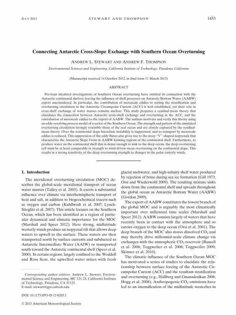
In Fig. 4a we present a Hovm€oller diagram of the

depth-averaged temperature uz5 h21

Ð 02h udz in our ref-

erence simulation at y 5 300km. The ubiquitous streaks

of relatively warm and cold water correspond to eddies

crossing this line of latitude southward and northward,

respectively. Zhang et al. (2011) found similar patterns

FIG. 2. Time- and zonal-mean zonal velocity u of our reference

simulation in statistically steady state. The contour interval is

2 cm s21 and the u5 0 contour is plotted in white.

FIG. 3. (a)Mean stratification and (b) residual overturning streamfunction for our reference simulation. In (b) the dotted and solid lines

highlight positive and negative streamlines respectively, with a contour interval of 0.25m2 s21. An overturning of 1m2 s21 corresponds to

1 Sv over the 1000-km channel length.


of tracer export from a bay on the continental shelf

in an idealized two-layer configuration. Export of the

coldest water is concentrated between x’2100 km and

x ’ 250 km, centered around 75 km eastward of the

most rapid bottom water formation at x5 0. This is due

to advection of eddies by the mean zonal velocity, which

is around 2 cms21 at this latitude and is visualized by the

diagonal streaks in Fig. 4a.

We quantify the eddy heat transport in Fig. 4b by

defining the vertically integrated meridional heat flux

qyt 5

ðz50

z52hdz yu

t5

ðz50

z52hdz (ytu

t1 y0u0

t) , (7)

which we have decomposed into mean and ‘‘eddy’’

components. Here primes denote deviations from the

time mean, for example, u0 5 u2 ut. The time average is

taken over 130 years in statistically steady state to mini-

mize the influence of topographic Rossby waves whose

propagation speeds are very close to that of the slope

current. The imposed cooling on the shelf leads to a

patch of denser water forming in the region x2 1 y2 ( Lc,

visible in Fig. 1. This gives rise to a mean eastward baro-

clinic flow, via thermal wind balance, that transports

water off the shelf in x , 0 and onto the shelf in x . 0.

This accounts for the zonal asymmetry in the mean

component of qyt in Fig. 4b. The eddy component of

qyt is everywhere negative and corresponds to a south-

ward heat transport that is most intense at x ’ 75km,

as suggested by Fig. 4a.

In Fig. 4c we plot the time- and zonal-mean meridio-

nal heat flux qy as a function of latitude. The northern

surface heating and southern surface/shelf cooling lead

to a southward heat transport over most of the domain.

In the ACC, the net heat flux is small compared to the

large northward mean and southward eddy heat fluxes.

On the continental shelf the heat transport is dominated

by eddies, transporting cold water northward to the shelf

break. On the continental slope the eddy heat transport

vanishes, and downslope flow takes place in a frictional

bottom boundary layer. The mean down-slope velocity

between y5 400 km and y5 600 km is 0.9 cms21, and the

mean along-slope velocity is 20.63 cms21. Outflowing

dense water takes around 403 days to traverse the slope,

during which it travels around 2300km westward.

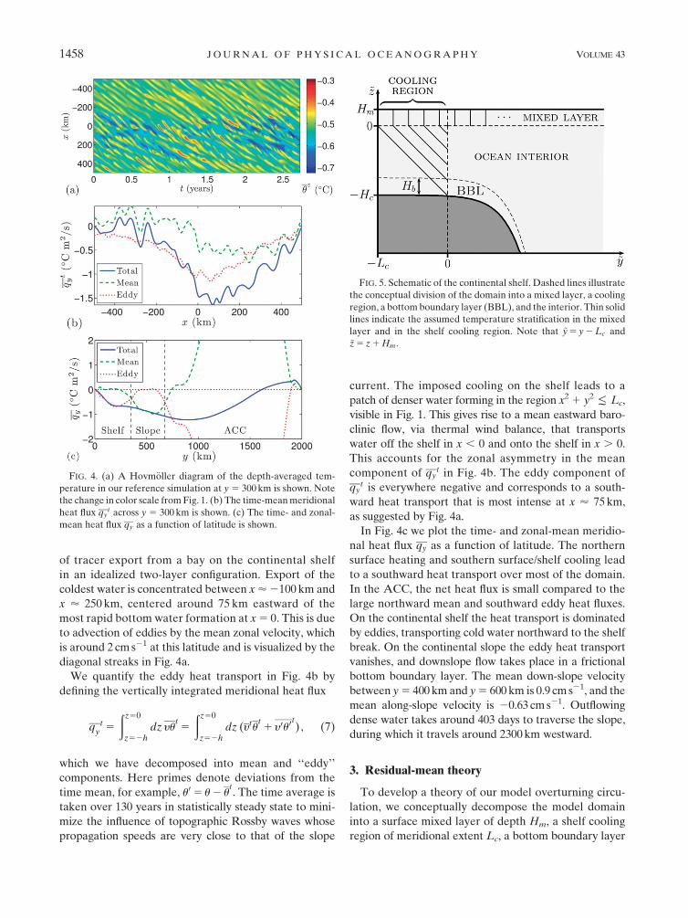
3. Residual-mean theory

To develop a theory of our model overturning circu-

lation, we conceptually decompose the model domain

into a surface mixed layer of depth Hm, a shelf cooling

region of meridional extent Lc, a bottom boundary layer

FIG. 4. (a) A Hovm€oller diagram of the depth-averaged tem-

perature in our reference simulation at y 5 300km is shown. Note

the change in color scale fromFig. 1. (b) The time-meanmeridional

heat flux qyt across y 5 300 km is shown. (c) The time- and zonal-

mean heat flux qy as a function of latitude is shown.

FIG. 5. Schematic of the continental shelf. Dashed lines illustrate

the conceptual division of the domain into a mixed layer, a cooling

region, a bottom boundary layer (BBL), and the interior. Thin solid

lines indicate the assumed temperature stratification in the mixed

layer and in the shelf cooling region. Note that ~y5 y2Lc and

~z5 z1Hm.


of thickness Hb, and the ocean interior. Figure 5 illus-

trates this decomposition and the assumed temperature

stratification in the surface mixed layer and shelf cooling

region. For convenience we define a translated system of

Cartesian coordinates (~y, ~z)5 (y2Lc, z1Hm), in which

(0, 0) lies at the upper southern corner of the ocean interior.

a. Residual-mean equations

We derive the core equations of residual-mean theory

following Marshall and Radko (2003, 2006). Averaging

the material conservation equation for temperature, we

obtain

J(cy, u)5 Su1$ � (k$u) and cy5c1c+ , (8)

where $[ (›~y, ›

~z) is the two-dimensional gradient opera-

tor. The mean temperature u is advected by the residual

streamfunction, subject tomean temperature sources/sinks

Su and mixing k across temperature surfaces. Following

Marshall and Radko (2003), we relate the mean stream-

function c in the ocean interior to the surface wind stress,

c52t(~y)

r0f0, (9)

which is valid in our zonally periodic domain in the

limit of vanishingly small Rossby number and viscosity.

We have also approximated f by its reference value f0.

The eddy streamfunction c+ and diapycnal diffusivity

k are defined as the components of the advective eddy

heat flux directed along and across mean isotherms, re-

spectively (Plumb and Ferrari 2005),

c+5y0u03$u

j$uj2and k52

y0u0 � $uj$uj2

. (10)

To close (8) we parameterize the eddy heat flux y0u0 fol-lowingGent andMcWilliams (1990), assuming that eddies

transport heat down the meridional temperature gradient,

y0u052K›u

›~y, 0 c+5 (K2 k)su . (11)

Here K . 0 is the isopycnal or eddy diffusivity and

su 52›~yu/›

~zu is the isotherm slope. This definition of

c+ differs from that used byMarshall and Radko (2003)

by a term proportional to k. We will later neglect this

term under the assumption of small aspect ratio.

A basic constraint on the streamfunctions c and c+ is

that the instantaneous mass and heat transports through

solid boundaries should be zero. In our zonally symmetric

domain this constraint may be satisfied by imposing

c5 0, c+5 0 and $u � n5 0 on ›S , (12)

where ›S denotes the domain boundary and n denotes

the unit normal vector. In the appendix we employ (12)

to derive boundary conditions for the surface mixed

layer, the shelf cooling region, the ocean bed, and the

northern relaxation region.

b. Nondimensionalization

To simplify our analysis of the residual-mean (8), we

nondimensionalize using the following scales (Nikurashin

and Vallis 2011):

cy, c+, c ;t0

r0j f0j, ~y; ~Ly, ~z; ~H, t; t0, u; u0,

Qm ;u0t0

r0j f0j ~Ly

, Vc ;t0

r0j f0j ~H, k5k0k,

K5~Lyt0

~Hr0j f0jL, «5

k0~Lyr0j f0j~Ht0

, and m5~H~Ly

.

(13)

Here ~H5H2Hm, k0 . 0, t0 . 0, and f0 , 0 are scales

for the depth, diapycnal diffusivity, wind stress and

Coriolis parameter, respectively. The downward surface

heat flux Qm and shelf piston velocity Vc are defined

in the appendix. We denote dimensionless variables

using a hat. The dimensionless isopycnal and diapycnal

diffusivities, L and k, may vary arbitrarily and will be

discussed in section 4. For typical parameter values of

K 5 2000m2 s21, k0 5 1 3 1024m2 s21, t0 5 0.2Nm22,

and f0 5 13 1024 s21, we obtain L ’ 1.7, «5 33 1022,

and m ’ 1.7 3 1023. Neglecting terms of O(m2) through-

out, the dimensionless residual-mean equations and

boundary conditions may be summarized as

J(cy, u)5 «

›

›zk›u

›z

� �, (14a)

cy5 c1 c

+, c

+5LsuFb(z), c5 tFb(z) , (14b)

cy(y, 0)5

›u

›y(y, 0)

" #21

Qm(y) , (14c)

cy(0, z)5 Vc

[u(0, z)2 uc]

›zu(0, z)I(z) , (14d)

›u

›z(0, 2h)5 0, and (14e)

u(12 Ln, z)5 un(z) . (14f)

The derivation of boundary conditions (14c)–(14f) is

given in the appendix as are the definitions of the ver-

tical structure functions Fb(z) and I(z).


4. Isopycnal and diapycnal diffusivities

In this section we develop a parameterization for K

and k that is suitable for our model problem. Ideally

our theory should not be conditioned by our simulations,

so that their results may be fairly compared. However,

our simulations exhibit dramatic changes in K over the

continental slope, and in k close to the ocean bed, which

our theory must address to capture key features of the

stratification and overturning circulation. We therefore

motivate parameterizations of K and k using our refer-

ence simulation, described in section 2, and then test

the theory against simulations with a range of different

surface wind stress profiles in section 6. In this section we

return to dimensional variables for convenience.

a. Eddy fluxes over the continental slope

Recent studies using numerical simulations (Isachsen

2011) and laboratory experiments (Pennel et al. 2012)

have shown that sloping topography may stabilize coastal

currents because it suppresses baroclinic instability. Fol-

lowing Isachsen (2011) and Pennel et al. (2012), we quan-

tify this effect using the topographic parameter d,

d5sbsu, (15)

where sb 5 2dyh and su 52›yu/›zu as in section 3.

Isachsen (2011) constructed an eddy diffusivity using the

growth rates of the Eady problem over a sloping bottom

using the approach of Stone (1972),

K(d)}max(s) � l2js5max(s) . (16)

Here s is the growth rate, and l is the wavelength. In

Fig. 6 we plot K against d, as diagnosed from our ref-

erence simulation at all points in the y/z plane via (11),

excluding those in the surface mixed layer and in the

lowest grid cells. We also plot the theoretical diffusivity

(16) from the two-layer quasigeostrophic (QG) equa-

tions with equal layer depths (see e.g., Pavec et al. 2005;

Pennel et al. 2012), rescaled to fit the simulation data

approximately.

The diagnosedK in Fig. 6 is qualitatively similar to the

results of Isachsen (2011) for d$ 0, but differs for d, 0.

In our simulations the baroclinic stability may be altered

by the strong depth-dependence of the isopycnal slope

su in regions where d, 0, in contrast to the experiments

of Isachsen (2011). The QG theory predicts that K

should be zero for d . 1, and that K / 0 as d / 2‘,whereas the diagnosed K is nonzero as d / 6‘. Thisresults in the smooth temperature extrema over the

continental shelf in Fig. 3a. However, it should be noted

that the variation in depth in our simulations lies well

outside the range of validity of QG theory.

Further work is required to develop an accurate pa-

rameterization of eddy transports over the continental

slope, but such an undertaking is beyond the scope of

this paper. Instead, we parameterize heuristically the

dramatic reduction in K when sb becomes comparable

to su. Our goal is to capture the key features of K(d) in

our reference simulation in order to develop a simple

theory of the model’s overturning and stratification.

Specifically, we choose

K5K0

�11

1

2

ffiffiffiffiffiffiffiffiffiffiffiffiffiffiffiffiffiffiffiffiffiffiffiffiffiffiffiffiffiffiffiffiffiffiffiffiffiffiffi(12 jdj)21 4g2jdj2

q

21

2

ffiffiffiffiffiffiffiffiffiffiffiffiffiffiffiffiffiffiffiffiffiffiffiffiffiffiffiffiffiffiffiffiffiffiffiffiffiffiffi(11 jdj)21 4g2jdj2

q �, (17)

where g � 1 and K0 is constant. When g 5 0, (17)

simplifies toK5K0(12 jdj)H(12 jdj), whereH denotes

the Heaviside function. In this case K 5 0 for jdj . 1,

similar to theQG theory when d. 0. For nonzero g, (17)

has the property thatK5 gK01O(g2) for d5 1, soK is

reduced by a factor of g when the isopycnal and topo-

graphic slopes have the same magnitude. In the limit

d / 6‘, (17) asymptotes to K / 2g2K0. In Fig. 6 we

plot (17) for the case g 5 0.05; we use this value in all

solutions presented in this paper.

b. Deep diapycnal mixing

In our simulations we prescribe a uniform vertical

diffusivity of ky 5 5 3 1026m2 s21, so cross-isopycnal

FIG. 6. Eddy diffusivity K diagnosed via (11) from our reference

simulation (points), constructed via (16) from two-layer baroclinic

instability theory (dashed line), and as given by our parameteri-

zation (17) with K0 5 2000m2 s21 (solid line). There are few di-

agnosed values of K between d 5 23 and d 5 0 because in this

simulation the isotherm slope is only positive where the conti-

nental slope is very steep.


flow in the deep ocean is achieved via a combination of

convective mixing and grid-scale numerical diffusion be-

cause of the flux-limited temperature advection scheme.

In Fig. 7 we plot as a function of depth the mean diffu-

sivity supplied by KPP (kKPP), where the mean has been

taken in x, t, and over y 2 (800km, 1900km). For com-

parison, we also plot the diffusivity diagnosed directly

from the cross-isotherm component of the mean me-

ridional and vertical eddy heat fluxes (kmean) via (10).

The rapid increase in k close to the ocean bed results

in a diffusive heat sink on the right-hand side of (14a),

which must be balanced by residual advection down the

mean temperature gradient. This gives rise to the in-

tense (;1.7m2 s21) recirculating overturning cell visible

at the bottom of Fig. 3b. The magnitude of kmean, and

therefore of the deep recirculation, may be reduced by

increasing the vertical resolution and employing an al-

ternative temperature advection scheme (see Hill et al.

2012). However, these modifications change c by at

most 1%–2% everywhere else in the domain, particu-

larly over the continental shelf and slope.

The diagnosed diffusivity profiles kKPP and kmean mo-

tivate the following choice of k for RMT,

k(y, z)5k011

2(kb 2 k0)

�12 tanh

�z1 h2Zk

Hk

��,

(18)

where k0 5 5 3 1026m2 s21, kb 5 1 3 103m2 s21, Zk 5250m, and Hk 5 50m. The diffusivity profile in the

ACC is shown in Fig. 7. This parameterized deep dia-

pycnal mixing may be viewed as an artifice of our nu-

merical configuration. However, strong diapycnal mixing

is required for bottom water to cross isopycnals close to

the ocean bed (Ito and Marshall 2008), and k has been

observed to increase by two or more orders of magni-

tude in parts of the Southern Ocean (Garabato et al.

2004). Furthermore, our residual-mean solutions in sec-

tion 5 develop unrealistically strong stratification un-

less k is comparable to the profile shown in Fig. 7.

5. Solution of the residual-mean equations

a. Numerical solutions in terrain-followingcoordinates

We create an iterative scheme to solve (14a)–(14f) by

introducing an artificial time derivative into (14a), fol-

lowing Nikurashin and Vallis (2011, 2012),

›u

›t1 J(c

y, u)5 «

›

›zk›u

›z

!. (19)

Here the scale for time t is r0jf0jL ~H/t0 ; 80 yr. We re-

write u as a function of y and z, where z 5 (z/h)H is

a terrain-following vertical coordinate, then discretize

(19) on an Arakawa C grid and apply the finite-volume

scheme of Kurganov and Tadmor (2000). We integrate

forward in time using the total variation diminishing

Runge-Kutta scheme of Shu and Osher (1989) until the

computation reaches a steady state.

In Fig. 8 we plot the stratification and overturning

circulation computed using parameters appropriate to

our reference simulation, with K0 5 2000m2 s21. This

solution, and all of those described below in section 6,

has been computed on a numerical grid of 150 3 150

points. Our theory captures the qualitative features of

the stratification and overturning circulation through-

out the domain. The region of anomalously weak over-

turning adjacent to the continental slope is due to our

simplified parameterization in (18) of deep diapycnal

mixing. This region may be corrected using a more so-

phisticated parameterization that permits latitudinal

variation of kb,Hk, andZk, but it has little impact on our

results. Both our theory and our eddy-resolving simula-

tions predict upper and lower overturning cell strengths

of around 0.6m2 s21 and 0.5m2 s21. In section 6 we

quantify the predictive skill of our theory over a range

of surface wind stress profiles.

b. Structure of the Antarctic Slope Front

In the limit of vanishingly small diapycnal mixing

(« / 0), the residual-mean temperature (14a) may be

solved asymptotically along individual isotherms.

We rewrite (14a)–(14f) in y/u coordinates via the trans-

formation z5 z(y, u), cy5 c

y[y, z(y, u)], under which the

isotherm slope su may be written as

FIG. 7. Mean vertical diffusivity profiles supplied by KPP

(points) and diagnosed directly from the heat fluxes in our refer-

ence simulation (dashed–dotted line), and our theoretical param-

eterization in (18) of k (solid line).


›z

›y u

5 su 52›yu

›zu.

�� (20)

We will integrate this equation to determine the shapes

of isotherms that originate from the shelf cooling re-

gion at y5 0. The isotherm slope su is determined via

(14b) as

suL(su)5 cy(y, u)2 t(y) . (21)

Here we assume for simplicity that the isotherm enters

neither the bottom boundary layer nor the surface

mixed layer, so Fb(z)[ 1. To determine the change in cy

along the isotherm, we use (20) to write the Jacobian

J(cy, u) as

J(cy, u)5

›u

›z

›cy

›y z

1 su›c

y

›z y

��!5

›u

›z

›cy

›y u

,

��

(22)

where the rightmost equality follows from an application

of the chain rule. Substituting (22) into (14a) yields an

equation for the rate of change of cyalong isotherms,

which we solve via an asymptotic expansion in «,

›cy

›y u5O(«)0c

y5 c

y0(u)1O(«) ,

�� (23)

where cy0(u)5 c

y[0, z(0, u)]# 0 by the shelf boundary

condition (14d).

As L . 0 for all d, it follows from (21) that the sign

of the isotherm slope is determined by the relative

strengths of the mean and residual streamfunctions, or

sign(su)5 sign(cy0 2 t) to leading order in «. If the re-

sidual streamfunction is stronger than the wind-driven

overturning on the slope, cy0(u), tACC 5miny(t), then

su , 0 for all y, and so the isotherm does not form a

V shape. This accurately describes the coldest isotherms

emanating from the shelf in Figs. 3a and 8a. If the re-

sidual streamfunction is weaker than the wind-driven

overturning on the slope, tACC , cy0 , 0, then the form

of the surface wind stress (4) means that su changes sign

twice between y5 0 and y5 LASF. This presents as a

V-shaped ASF in Figs. 3a and 8a. The sharpness of the

V is accentuated because of the reduction in L by a

factor of around 40 over the continental slope, due to

suppression of baroclinic instability (Isachsen 2011).

To emphasize the role of eddy suppression in shaping

the ASF, in Fig. 9a we plot the residual-mean stratifi-

cation produced by a uniform isopycnal diffusivity. The

shelf and slope stratification no longer resembles the

structure diagnosed from our reference simulation (see

Fig. 3), and the warmer shelf water doubles the strength

of the deep overturning circulation (not shown). If there

is no bottom water formation on the shelf [cy(0, z)[ 0]

then (21) yields su . 0. In this case the isotherms origi-

nating from the northern boundary would simply plunge

into the continental slope, as observed in the Eastern

Weddell Sea (Chavanne et al. 2010) and other parts of

the Antarctic margins where the continental shelf is

narrow (Whitworth et al. 1998). This configuration is

illustrated in Fig. 9b, which shows the residual-mean

stratification produced by setting the surface buoyancy

forcing and shelf cooling to zero.

c. A constraint on the deep overturning strength

Even under an expansion in « the system (20)–(21)

remains analytically intractable. We therefore pose an

additional asymptotic expansion of our isopycnal diffu-

sivity L in the parameter g,

L(su)5L0(12 jdj)H(12 jdj)1O(g2) , (24)

where d5 sb/su as in section 4. Substituting this expan-

sion into (21) yields

FIG. 8. As in Fig. 3, but with u and cy calculated numerically via RMT using (19). Units are dimensional.


su5cy02 t

L0

1 sign(cy02 t)jsbj1O(«, g2) . (25)

Substituting this approximation into (20), wemay integrate

exactly to obtain the change in isotherm height above the

ocean bed between the southern and northern boundaries,

(z1 h)y51

y5051

L0

cy02

1

2tASFLASF 2

1

2tACCLACC

!

1 2(12 Hs) tanhjLASF

2Ws

!1O(«,g2) ,

(26)

where Hs 5 ~Hs/H is the dimensionless shelf depth ex-

cluding the surface mixed layer. Here we have ignored

the relaxation region close to the northern boundary for

simplicity, and the parameter j is defined as

j5

8>>>>>><>>>>>>:

2

pcos21

ffiffiffiffiffiffiffifficy0

tASF

vuut0B@

1CA , tASF # c

y0, 0,

0, cy0 # tASF .

(27)

Because of the formation of dense water on the con-

tinental shelf, colder water exists at the southern bound-

ary than at the northern boundary. In y/u coordinates, any

isotherm z(y, u) that originates from these depths at the

southern boundary [z(0, u), z0] must enter the bottom

boundary layer before it reaches y5 1, so we require

that z(1, u), 21. A necessary condition is that the left-

hand side of (26) must be less than zero. Therefore, the

right-hand side of (26) must be less than zero, to leading

order in « and g2. This serves to constrain the strength of

the deep overturning circulation, measured by cy0. By set-

ting the right-hand side of (26) to zero and solving for cy0,

we predict the sensitivity of the deep overturning cir-

culation to changes in the polar easterlies tASF. In section

6 this prediction is compared with those of our numerical

RMT solutions and our eddy-resolving simulations. The

last term on the right-hand side of (26) typically domi-

nates the others unless j 5 0, so an approximate con-

straint is that cy0(u)& tASF, or in dimensionless variables,

max~y50

jcyj*��tASF

r0 f0

��5CASF . (28)

This states that in order to formwater on the continental

shelf that is dense enough to sink to the deep ocean bed,

the overturning must be stronger than the wind-driven

Ekman overturning circulation in the ASF. Note that if

condition (28) is satisfied then the deepest isotherms

originating from ~y5 0 do not form a V as they cross the

continental slope, as explained in the previous sub-

section. These results are summarized in section 7.

6. Sensitivity to surface wind stress

We now investigate the sensitivity of our eddy-

resolving simulations and residual-mean model to changes

in the surface wind stress. We define three sets of sen-

sitivity experiments by varying the wind stress parame-

ters tACC and tASF about their reference values.

a. Zonal transport

The zonal transport is the most fundamental measure

of the ACC and ASF, which are clearly identified in

FIG. 9. Plots of the residual-mean temperature stratification, corresponding to our reference simulation with alternative parameter

choices. In (a) we have assumed a uniform isopycnal diffusivity K5 2000m2 s21 everywhere, including over the continental slope. In (b)

we have turned off the forcing on the continental shelf (Vc 5 0, see the appendix) and at the ocean surface (Qm 5 0), so the residual

overturning is vanishingly small.


the mean zonal velocity u for our reference simulation,

shown in Fig. 2. We determine the zonal transport in

our residual-mean solutions from the temperature strat-

ification via thermal-wind balance,

u5 ub 2ag

f0

ðz2h

›u

›ydz0 and ub 5

t

r0rb. (29)

Here we have assumed that at each latitude, the mean

basal velocity ub 5 ujz52h extracts all momentum input

by surface wind stress via bottom friction. It would be

more realistic to prescribe ujz52h1Hband assume that

the wind-input momentum is removed by viscous stress

in the bottom boundary layer of thicknessHb, but (29) is

a good approximation.

In Fig. 10a we plot the response of the zonal transport

in the ACC, defined as 800 # y # 1900 km, to changes

in the midlatitude westerly wind strength tACC. The

barotropic component is simply the basal velocity, and

is slightly smaller in the RMT solutions than in our

simulations. The baroclinic transport in our simulations

is almost completely independent of tACC, indicating

that our model ACC is in an ‘‘eddy saturated’’ regime

(Meredith et al. 2011). This is partially a consequence

of the thermal relaxation at the southern and northern

boundaries, which inevitably leads to a meridional tem-

perature gradient across the domain. In RMT, the iso-

therm slope is given by (21). In the ACC K [ K0 is

constant and c typically dominates cy, so K0 must vary

approximately linearly with tACC in order to leave suunchanged. We therefore prescribe the eddy diffusivity

scale K0 in (17) as

K05Kref

tACC

tref, (30)

where Kref 5 2000m2 s21 and tref 5 0.2Nm22. The re-

sulting RMT-predicted stratification yields a baroclinic

zonal velocity that agrees very closely with our simula-

tions, as shown in Fig. 10a. We obtained equivalent

RMT solutions that hold K0 fixed across all values of

tACC, and found that the baroclinic transport varied

by around 40 Sv between tASF 5 0.1Nm22 and tASF 50.3Nm22.

In Fig. 10b we plot the response of the zonal trans-

port over the continental slope, defined as 200 # y #

800 km, to changes in the polar easterly wind strength

tACC. The net transport is close to zero in our reference

simulation because of the surface-intensified eastward

jets surrounding the ASF, visible in Fig. 2. In this case

the RMT barotropic velocity is consistently around 25%

smaller than the basal velocity in our simulations. This is

due to a net northward flux of zonal momentum from the

slope to the ACC, resulting in the basal velocities in

both regions exceeding that predicted by (29). The

discrepancy is more noticeable in Fig. 10b because of

the smaller volume of the slope region. The baroclinic

slope transports follow qualitatively similar patterns, but

RMT consistently predicts a transport that is 30–50 Sv

too large. This arises because the residual-mean solu-

tions tend to form sharper temperature gradients close

to the topography at the shelf break, resulting in a larger

positive zonal velocity throughout the water column

above. For tASF $ 0 the baroclinic transport is in-

sensitive to the wind stress, and the stratification and

overturning closely resemble those shown in Fig. 11.

b. Overturning circulation

The MOC in our eddy-resolving simulations has a

broadly similar presentation to that shown in Fig. 3b for

all parameter combinations considered here.Wequantify

FIG. 10. Sensitivity of the zonal transport (a) in the ACC (800# y# 1900 km) and (b) over the slope (200# y# 800 km) to changes in

the westerly wind strength tACC and easterly wind strength tASF respectively. The vertical dashed lines indicate our reference simulation

from section 2.


the strength of the upper overturning cell following

Abernathey et al. (2011), defining Cupper as the largest

value of cy anywhere in the domain. We quantify the

lower overturning cell following Stewart and Thompson

(2012); we restrict our attention to streamlines that extend

from the shelf cooling region at y5 200km to y5 1900km.

We then defineClower as the largest negative value of cy

over all such streamlines. This excludes the influence of

the deep recirculation visible in Fig. 3b, andmeasures the

net transport from the southernmost to the northernmost

edges of the model Southern Ocean.

Figure 12a shows the response ofCupper andClower to

changes in tACC, where again K0 is prescribed following

(30). The upper overturning cell exhibits a modest sensi-

tivity to changes in the midlatitude westerlies in our sim-

ulations, with a least squares slope of 1.39m4 s21 N21.

Abernathey et al. (2011) obtained a somewhat larger

sensitivity of 2.6m4 s21 N21 using fixed surface buoy-

ancy fluxes. This discrepancy may be due to the range

of temperatures spanned by the upper cell, determined

by the northern boundary condition, and the relative

positions of the wind stress and surface heat flux max-

ima. The simulated stratification and overturning over

the continental shelf and slope are not modified by

changes in tACC, so Clower is relatively insensitive. In

RMTCupper has a similar magnitude and increases with

tACC, but the least squares sensitivity of 0.78m4 s21N21

is only around half of that in the simulations. This dis-

crepancy arises because the upper overturning is set at

the surface by (14c), and the surface heat flux Qm(y) is

prescribed by (3) over all of our RMT solutions. Thus

changes in Cupper are due entirely to the surface tem-

perature gradient, which differs visibly in Figs. 3a and 8.

A more sophisticated parameterization of the ACC eddy

diffusivity K is required to capture the surface tempera-

ture gradient accurately, and thus predict the sensitivity

of Cupper to changes in tACC.

Figure 12b shows that in both our simulations and

in our RMT, Cupper is insensitive changes in tASF.

MeanwhileClower varies rapidly for tASF , 0, with our

GCM and RMT predicting least squares sensitivities of

5.97m4 s21N21 and 6.44m4 s21N21, respectively. We

also plot the asymptotically derived constraint on Clower

FIG. 11. As in Fig. 3, but for tASF 5 0.

FIG. 12. Sensitivity of the overturning circulation to changes

in (a) the westerly wind strength tACC and (b) the easterly wind

strength tASF.


from section 5, obtained by setting the right-hand side of

(26) to zero. This constraint predicts a stronger sensitivity

of 9.80m4 s21N21, very close to that of the wind-driven

mean overturning c over the slope. This discrepancy is

due to the neglect of diapycnal mixing in (26), which in-

tensifies the deep overturning close to the ocean bed.

For tASF $ 0 the deep overturning is largely driven by

surface heat flux, as shown in Fig. 11. In this regime the

stratification is insensitive to tASF due to eddy saturation

over the continental slope, as shown in Fig. 10b, and the

surface heat flux Qm is fixed. Thus Clower also becomes

insensitive to tASF. Our RMT solutions substantially

overpredict the magnitude of Clower in this regime be-

cause the simulated isotherms on the shelf become too

steep to be described by a constant eddy diffusivity K0.

c. Cross-shelf heat flux

Figure 13 shows the zonally averaged cross-shelf heat

flux qy for various wind strengths tASF over the conti-

nental slope (cf. Fig. 4). As in our reference simulation,

the eddy component of qy is much larger than the mean

component for all values of tASF. It is unsurprising that

the eddy heat flux follows a similar pattern to Clower

because the overturning on the shelf is due to the ex-

change of warm and cold eddies across the shelf break,

as shown in Fig. 4. As y is confined to the surface mixed

layer and bottom boundary, the mean heat flux may be

expected to be approximately proportional to tASF and

to the temperature difference between the surface and

the shelf. The shelf waters become weakly stratified for

tASF $ 0, as shown in Fig. 11, resulting in only a small

northward heat flux in this regime. Thus the net heat flux

varies more rapidly with tASF , 0 than with tASF $ 0.

This is consistent with the hypothesis that warm CDW

inflow to the Ross and Amundsen Seas is controlled by

seasonal changes in the offshore easterlies (Thoma et al.

2010; Dinniman et al. 2011), but seems to contradict the

idea that changes in offshore westerly wind stress con-

trol CDW intrusions into the Amundsen Sea (Thoma

et al. 2008).

7. Conclusions

In this study we have developed eddy-resolving sim-

ulations and a residual-mean theory for an idealized

sector of the Southern Ocean, including a representation

of the Antarctic continental shelf and slope. Our theory

includes boundary conditions for the surfacemixed layer,

the shelf cooling region, the bottom boundary layer, and

the northern relaxation region. Our simulations exhibit

suppression of baroclinic instability over the continental

slope, and strong diapycnal mixing close to the ocean

bed. These effects could not be predicted a priori and are

critical features of the dynamics in this system, so our

theory incorporates simple parameterizations for the

isopycnal and diapycnal diffusivities K and k based on

our reference simulation. Away from these regions K

and k are held constant, yet the mean stratification and

overturning in Fig. 8 agrees convincingly with those di-

agnosed from of our reference simulation in Fig. 3. This

study reinforces the importance of resolving mesoscale

eddies over the continental slope, or at least employing

a careful parameterization of their transport. The most

frequently used parameterizations of K would not cap-

ture the behavior of the eddies in our simulations (see

Isachsen 2011), and may be expected to produce a quali-

tatively different stratification, more closely resembling

Fig. 9a than Figs. 3a or 8a. Indeed, Fig. 9a suggests that

it is the suppression of baroclinic eddies over the con-

tinental slope that permits our model ocean to form its

densest water on the continental shelf.

Residual-mean theory intuitively explains the sharp

V-shaped isopycnal structure that characterizes theASF

in bottom water-forming regions of the Antarctic con-

tinental shelf (e.g., Thompson and Heywood 2008) as

the result of suppression of baroclinic instability over

the continental slope. The theory also accounts for

stretches of the continental shelf where little or no dense

water is formed, and the shoreward side of the V is

absent (Whitworth et al. 1998), as illustrated in Fig. 9b.

Both our residual-mean solutions and our eddy-resolving

simulations predict that the strength of the deep over-

turning circulation is constrained to be at least compa-

rable in strength to the Ekman transport driven by the

polar easterly winds. In section 5 we showed via (28) that

this is approximately equivalent to requiring that the

densest isopycnals emanating from the continental shelf

do not form a V shape, but rather sink down the conti-

nental slope and outcrop at the ocean bed. The existence

FIG. 13. Sensitivity of the meridional heat flux across the shelf

break (y 5 300 km) to changes in the wind stress tASF over the

continental slope.


of such isopycnals is necessary to support denser waters

on the shelf than at the northern boundary. These key

results are illustrated schematically in Fig. 14.

There are a number of potential improvements to

the admittedly idealized model described in this study,

which would help to generate more realistic flows. For

example, zonal variations in the bottom topography con-

stitute an important omission from our model configu-

ration. Submarine canyons may support geostrophic

mean cross-slope transports or turbulent down-slope cur-

rents, providing an alternative route for AABW to es-

cape the continental shelf, and deep-ocean ridges may

support geostrophic transport of AABW across the

ACC (e.g., Naveira Garabato et al. 2002). Such fea-

tures could substantially alter the influence of the polar

easterlies on the deep overturning cell, and require

further investigation. Another desirable addition would

be the dependence of density on salinity, which is par-

ticularly pronounced over the Antarctic continental shelf

because of nonlinearities in the equation of state (Gill

1973). With sufficient resolution the importance of the

thermobaric effect on dense water formation and ex-

port could also be explored. Incorporation of sea ice

and ice sheets adds considerable complexity but would

ultimately provide further insight into the dynamical

processes governing cross-shelf exchange. We purpose-

fully kept our residual-mean model as simple as possible

to permit a fair comparison with our simulations, and

there is certainly scope for improving our parameteri-

zations of the eddy and diapycnal diffusivities. For ex-

ample, the simulated eddy diffusivity K is accurately

described by the parameterization of Visbeck et al. (1997)

everywhere except over the continental slope. While all

of these aspects would entail significant modifications to

the theory developed here, the success of RMT in re-

producing the stratification and overturning in our sim-

ulations demonstrates its potential to explain complex

dynamical features like export of AABW and the struc-

ture of the ASF.

Acknowledgments.A.L.S.’s and A.F.T.’s research was

supported by the California Institute of Technology and

NSF Award OCE-1235488. The simulations presented

herein were conducted using the CITerra computing

cluster in the Division of Geological and Planetary Sci-

ences at the California Institute of Technology, and the

authors thank the CITerra technicians for facilitating

this work. The authors gratefully acknowledge the mod-

eling efforts of the MITgcm team. The authors thank

Dimitris Menemenlis, Christopher Wolfe, Rick Salmon,

Paul Dellar and Mike Dinniman for useful discussions.

The authors thank two anonymous reviewers for con-

structive criticisms that improved the original draft of

this manuscript.

FIG. 14. A schematic illustrating the formation of a V-shaped ASF and sensitivity of the deep

MOC to the easterly drivenmean overturningCASF. The ocean interior is approximately adiabatic,

socy ’cy(u). The red isotherm forms aV-shapedASFover the continental slopebecause thewind-

driven Ekman pumping deepens/shoals isotherms on the poleward/equatorward side of the ASF.

Theblue isothermmust insteadplungedown to the oceanbed to supply a sufficiently large poleward

eddy thickness flux over the continental slope, whereK is greatly reduced because of suppression of

baroclinic instability. Thus if denser water is to emanate from the shelf than exists at the northern

boundary, the deep MOC cy must be at least comparable to CASF on those isotherms.


APPENDIX

Boundary Conditions for Residual-Mean Theory

a. The surface mixed layer

As shown in in Fig. 5, we approximate the surface

mixed layer by assuming that the u is independent of

depth, u5 um(y) (Marshall and Radko 2003). Under this

assumption (8) becomes

2›cy

›~z

dumd~y

5›Q

›~z1

›

›~ykdumd~y

!, (A1)

where we have written the heat source Su as the vertical

divergence of a heat flux Q. We denote the surface heat

flux as Qj~z5Hm

5Qm(~y)52Q(~y)/r0Cp, where Cp 5 4 3103 J K21 kg21 is the specific heat capacity. We assume

that all of the surface heat flux is absorbed in the mixed

layer, so Q 5 0 at ~z5 0. To obtain a boundary condition

for c, we integrate (A1) from ~z5 0 to ~z5Hm using cy 50 at ~z5Hm,

cyj~z505

dumd~y

!21

Qm 1d

d~y

dumd~y

ðHm

0k d~z

!" #. (A2)

Thus the residual water mass exchange between the

ocean interior and the surface mixed layer is determined

by the surface heat input and meridional temperature

gradient.

b. The shelf cooling region

The water on the continental shelf is subject to direct

thermal relaxation to a temperature of uc 5 218C,

Su52T21(ut2 uc)

x, 2Lc # ~y# 0, (A3)

where the time scale T is given by (2). This thermal re-

laxation results in a zonal asymmetry in the time-mean

temperature of the shelf waters, visible in Fig. 1. To

evaluate (A3) exactly, we would need to prescribe the

three-dimensional temperature structure everywhere on

the shelf. Instead we derive an approximate boundary

condition for RMT under the assumption that the zonal

variations of utare small compared to its meridional and

vertical stratification. This amounts to replacing utwith u

in (A3), which may then be written as

Su’(~z2Hm)

ffiffiffiffip

pLc

2TcHsLx

exp 2~y1Lc1/2Lc

� �2" #(u2 uc) , (A4)

Here we have used expf2[x/(1/2)Lc]2g

x

’ffiffiffiffip

pLc/2Lx to

evaluate T21xfrom (2), which holds because Lc � Lx.

We further assume that the isotherm slope is uniform

in the cooling region, su [ sc 52 ~Hs/Lc, such that the

coldest isotherm connects (0, 2 ~Hs) to (2Lc, 0), as

shown in Fig. 5. The shelf temperature may therefore

be written as

u(~y, ~z)5 u(0, ~z2 sc~y), 2Lc# ~y# 0, (A5)

so both u and ›~zu are constant along each isotherm. This

assumption may seem restrictive, but in fact (A5) is

similar to themean shelf temperature in our simulations.

In sections 5–6 we show that the resulting boundary

streamfunction cy(0, ~z) agrees well with the simulated

overturning circulation over a range of wind stress

parameters.

In general, given Su(~y, ~z) and u(~y, ~z) everywhere in ~y 2(2Lc, 0) and ~z 2 (2 ~Hs,Hm), we may determine the

residual streamfunction cy(0, ~z0) at any depth ~z0. We

rewrite (8) as a derivative of cy along the contour

u5 u(0, ~z0) (e.g., Karsten and Marshall 2002),

›cy

›l5

Su1$ � (k$u)ffiffiffiffiffiffiffiffiffiffiffiffiffiffiffiffiffiffiffiffiffiffiffiffiffiffiffiffiffiffiffi(›~yu)

21 (›~zu)2

q , (A6)

where l is an along-contour coordinate. Scaling analysis

suggests that the direct cooling Su should dominate di-

apycnal mixing, and our simulations confirm that this is

the case. We therefore neglect the term proportional to

k in (A6). We also neglect the portion of each isotherm

that lies within the mixed layer, where (~z2Hm)/Hs � 1

is small and so the cooling Su is weak. Prescribing the

temperature of the shelf waters using (A5), (A6) may be

written as

cy(0, ~z0)5ð0~y0

d~ySu›~zu ~z5~z

01s

c~y.

�� (A7)

Here ~y0 5Lc~z0/ ~Hs is the position at which the isotherm

u5 u(0, ~z0) meets the mixed layer at ~z5 0. By assump-

tion (A5), u(~y, sc~y)5 u(0, ~z0) and ›~zu(~y, sc~y)5 ›

~zu(0, ~z0)

are constant along each isotherm, so we may integrate

(A7) exactly to obtain

cy(0, ~z)5Vc

[u(0, ~z)2 uc]

›~zu(0, ~z)I(~z) and Vc 5

ffiffiffiffip

pL2c~Hs

2TcHsLx

.

(A8)

Here Vc is a velocity scale for the heat flux across ~y5 0,

whose vertical structure is described by


I(~z)51

8fexp(24)2 exp[24(11 ~z/ ~Hs)

2]g

1

ffiffiffiffip

p

4 ~Hs

(~z1 ~Hs 2Hm)ferf(2)2 erf[2(11 ~z/ ~Hs)]g .

(A9)

Note that (12) still requires that cy[0, 2~h(0)]5 0 must

be satisfied at the bottom boundary.

c. The bottom boundary layer

To satisfy the no-flux boundary condition (12), the

wind-driven mean overturning c must adjust from its

interior form (9) to zero at ~z52~h(~y), where ~h5h2Hm. In the real ocean this is achieved via a bottom

Ekman layer, which may be described analytically un-

der the assumption of a negligible horizontal buoyancy

gradient (e.g., Pedlosky 1987; Vallis 2006). The bottom

Ekman layer is not resolved in our simulations, where

instead c is closed via a mean meridional transport

through the lowermost grid cells. We employ a simple

representation of the bottom boundary layer similar to

that of Ferrari et al. (2008),

c52t(~y)

r0 f0Fb(~z) , (A10)

where

Fb(~z)53

~zhHb

� �2

2 2~zhHb

� �3

, 0# ~zh#Hb ,

1 , Hb # ~zh # h .

8>><>>: (A11)

Here ~zh 5 ~z1 ~h is the height above the topography. This

form ensures that c is continuous and differentiable at

~z52 ~h1Hb, and that y5 0 at ~z52~h. As c+ describes

the mass transport due to geostrophic eddies, it should

also vanish in the ocean’s bottom Ekman layer. We

therefore prescribe

c+5KFb(~z)su , (A12)

which effectively reduces the eddy diffusivity K to zero

in the bottom boundary layer. To satisfy all parts of (12),

we also require

›u

›~z5 sb

›u

›~y, on ~z52~h , (A13)

where sb 52d~y~h is the slope of the bottom topography.

d. The northern boundary

In our simulations, the ocean temperature is relaxed

over the northernmost Ln 5 100 km of the domain to

a prescribed exponential profile (5),

Su52T21r

~y2 ~Ly1Ln

Ln

[u2 un(~z)] , (A14)

for ~y$ ~Ly 2Ln, where ~Ly 5Ly 2Lc. The region ~y 2( ~Ly 2Ln, ~Ly) may thus be included directly in the RMT

solutions described in section 5. However, in practice u

remains very close to un in this region, so for simplicity

we prescribe u( ~Ly 2Ln, ~z)5 un(~z).

REFERENCES

Abernathey, R., J. Marshall, and D. Ferreira, 2011: The de-

pendence of Southern Ocean meridional overturning on wind

stress. J. Phys. Oceanogr., 41, 2261–2278.

Andrews, D. G., J. R. Holton, and C. B. Leovy, 1987: Middle At-

mosphereDynamics. InternationalGeophysics Series, Vol. 40,

Academic Press, 489 pp.

Baines, P. G., 2009: A model for the structure of the Antarctic

Slope Front. Deep-Sea Res. II, 56 (13–14), 859–873.

Chavanne, C. P., K. J. Heywood, K. W. Nicholls, and I. Fer, 2010:

Observations of the Antarctic slope undercurrent in the

southeastern Weddell Sea. Geophys. Res. Lett., 37, L13601,

doi:10.1029/2010GL043603.

Dinniman, M. S., J. M. Klinck, and W. O. Smith, 2011: A model

study of Circumpolar Deep Water on the West Antarctic

Peninsula and Ross Sea continental shelves.Deep-Sea Res. II,

58, 1508–1523.D€o€os, K., and D. J. Webb, 1994: The Deacon cell and the other

meridional cells of the Southern Ocean. J. Phys. Oceanogr.,

24, 429–429.

Ferrari, R., J. C. McWilliams, V. M. Canuto, and M. Dubovikov,

2008: Parameterization of eddy fluxes near oceanic bound-

aries. J. Climate, 21, 2770–2789.

Ferreira, D., J. Marshall, and P. Heimbach, 2005: Estimating eddy

stresses by fitting dynamics to observations using a residual-

mean ocean circulationmodel and its adjoint. J. Phys.Oceanogr.,

35, 1891–1910.

Garabato, A. C. N., K. L. Polzin, B. A. King, K. J. Heywood, and

M. Visbeck, 2004: Widespread intense turbulent mixing in the

southern ocean. Science, 303, 210–213.

Gent, P. R., and J. C. McWilliams, 1990: Isopycnal mixing in ocean

circulation models. J. Phys. Oceanogr., 20, 150–155.

Gill, A. E., 1973: Circulation and bottom water production in the

Weddell Sea. Deep-Sea Res., 20, 111–140.

Gordon, A. L., 2009: Bottom water formation. Ocean Currents,

J. H. Steele, S. A. Thorpe, and K. K. Turekian, Eds., Associ-

ated Press, 263–269.

Hallberg, R., and A. Gnanadesikan, 2006: The role of eddies in

determining the structure and response of the wind-driven

Southern Hemisphere overturning: Results from the Model-

ing Eddies in the Southern Ocean (MESO) project. J. Phys.

Oceanogr., 36, 2232–2252.

Hill, C., D. Ferreira, J.M. Campin, J. Marshall, R. Abernathey, and

N. Barrier, 2012: Controlling spurious diapycnal mixing in


eddy-resolving height-coordinate ocean models—Insights

from virtual deliberate tracer release experiments. Ocean

Modell., 45, 14–26.

Hofmann, M., and M. A. M. Maqueda, 2011: The response of

Southern Ocean eddies to increased midlatitude westerlies:

A non-eddy resolving model study. Geophys. Res. Lett., 38,

L03605, doi:10.1029/2010GL045972.

Hogg, A. M. C., M. P. Meredith, J. R. Blundell, and C. Wilson,

2008: Eddy heat flux in the Southern Ocean: Response to

variable wind forcing. J. Climate, 21, 608–620.

Isachsen, P. E., 2011: Baroclinic instability and eddy tracer trans-

port across sloping bottom topography: How well does a

modified Eady model do in primitive equation simulations?

Ocean Modell., 39, 183–199.

Ito, T., and J. Marshall, 2008: Control of lower-limb overturn-

ing circulation in the Southern Ocean by diapycnal mixing and

mesoscale eddy transfer. J. Phys. Oceanogr., 38, 2832–2845.Jacobs, S. S., 1991: On the nature and significance of the Antarctic

Slope Front. Mar. Chem., 35, 9–24.

Karsten, R. H., and J. Marshall, 2002: Constructing the residual

circulation of the ACC from observations. J. Phys. Oceanogr.,

32, 3315–3327.Kitoh, A., S. Murakami, and H. Koide, 2001: A simulation of the

Last Glacial Maximum with a coupled atmosphere–ocean

GCM. Geophys. Res. Lett., 28, 2221–2224.

Krinner, G., and C. Genthon, 1998: GCM simulations of the Last

Glacial Maximum surface climate of Greenland and Antarc-

tica. Climate Dyn., 14, 741–758.

Kuhlbrodt, T., A.Griesel,M.Montoya,A. Levermann,M.Hofmann,

and S. Rahmstorf, 2007: On the driving processes of the At-

lantic meridional overturning circulation. Rev. Geophys., 45,

RG2001, doi:10.1029/2004RG000166.

Kuo, A., R.A. Plumb, and J.Marshall, 2005: TransformedEulerian-

mean theory. Part II: Potential vorticity homogenization and

the equilibrium of a wind-and buoyancy-driven zonal flow.

J. Phys. Oceanogr., 35, 175–187.

Kurganov, A., and E. Tadmor, 2000: New high-resolution central

schemes for nonlinear conservation laws and convection–

diffusion equations. J. Comput. Phys., 160, 241–282.Large, W. G., and S. G. Yeager, 2009: The global climatology of an

interannually varying air–sea flux data set. Climate Dyn., 33,

341–364.

——, J. C. McWilliams, and S. C. Doney, 1994: Oceanic vertical

mixing: A review and a model with a nonlocal boundary layer

parameterization. Rev. Geophys., 32, 363–404.

Lumpkin, R., and K. Speer, 2007: Global ocean meridional over-

turning. J. Phys. Oceanogr., 37, 2550–2562.Lynch-Stieglitz, J., and Coauthors, 2007: Atlantic meridional

overturning circulation during the last glacial maximum. Sci-

ence, 316, 66–69.

Marshall, J., and T. Radko, 2003: Residual-mean solutions for the

Antarctic Circumpolar Current and its associated overturning

circulation. J. Phys. Oceanogr., 33, 2341–2354.

——, and ——, 2006: A model of the upper branch of the meridi-

onal overturning of the Southern Ocean. Prog. Oceanogr.,

70 (2–4), 331–345.

——, and K. Speer, 2012: Closure of the meridional overturning

circulation through Southern Ocean upwelling. Nat. Geosci.,

5, 171–180.

——, A. Adcroft, C. Hill, L. Perelman, and C. Heisey, 1997a: A

finite-volume, incompressible Navier Stokes model for studies

of the ocean on parallel computers. J. Geophys. Res., 102 (C3),

5753–5766.

——, C. Hill, L. Perelman, and A. Adcroft, 1997b: Hydrostatic,

quasi-hydrostatic, and nonhydrostatic ocean modeling. J. Geo-

phys. Res., 102 (C3), 5733–5752.

McIntosh, P. C., and T. J. McDougall, 1996: Isopycnal averaging

and the residual mean circulation. J. Phys. Oceanogr., 26, 1655–

1660.

Meredith, M. P., A. C. Naveira Garabato, A. M. C. Hogg, and

R. Farneti, 2011: Sensitivity of the overturning circulation in

the Southern Ocean to decadal changes in wind forcing. J. Cli-

mate, 25, 99–110.Muench, R. D., and A. L. Gordon, 1995: Circulation and transport

of water along the western Weddell Sea margin. J. Geophys.

Res., 100 (C9), 18 503–18 515.

Naveira Garabato, A. C., E. L. McDonagh, D. P. Stevens, K. J.

Heywood, and R. J. Sanders, 2002: On the export of Antarctic

bottom water from the Weddell Sea. Deep-Sea Res. II, 49,

4715–4742.

Nikurashin, M., and G. Vallis, 2011: A theory of deep stratification

and overturning circulation in the ocean. J. Phys. Oceanogr.,

41, 485–502.——, and ——, 2012: A theory of the interhemispheric meridional

overturning circulation and associated stratification. J. Phys.

Oceanogr., 42, 1652–1667.

Nøst, O. A., M. Biuw, V. Tverberg, C. Lydersen, T. Hattermann,

Q. Zhou, L. H. Smedsrud, and K. M. Kovacs, 2011: Eddy

overturning of the Antarctic Slope Front controls glacial

melting in the Eastern Weddell Sea. J. Geophys. Res., 116,

C11014, doi:10.1029/2011JC006965.

Nowlin, W. D., Jr., and J. M. Klinck, 1986: The physics of the

Antarctic circumpolar current. Rev. Geophys., 24, 469–491.Olbers, D., andM. Visbeck, 2005: Amodel of the zonally averaged

stratification and overturning in the Southern Ocean. J. Phys.

Oceanogr., 35, 1190–1205.

Orsi, A. H., and C. L. Wiederwohl, 2009: A recount of Ross Sea

waters. Deep-Sea Res. II, 56 (13–14), 778–795.

——, S. S. Jacobs, A. L. Gordon, and M. Visbeck, 2001: Cooling

and ventilating the abyssal ocean. Geophys. Res. Lett., 28,

2923–2926.

Ou, H. W., 2007: Watermass properties of the Antarctic Slope

Front: A simple model. J. Phys. Oceanogr., 37, 50–59.Pavec,M., X. Carton, andG. Swaters, 2005: Baroclinic instability of

frontal geostrophic currents over a slope. J. Phys. Oceanogr.,

35, 911–918.

Pedlosky, J., 1987:Geophysical Fluid Dynamics. 2nd ed. Springer-

Verlag, 710 pp.

Pennel,R.,A. Stegner, andK.B�eranger, 2012: Shelf impact onbuoyant

coastal current instabilities. J. Phys. Oceanogr., 42, 39–61.

Plumb, R. A., and R. Ferrari, 2005: Transformed Eulerian-mean

theory. Part I: Nonquasigeostrophic theory for eddies on a

zonal-mean flow. J. Phys. Oceanogr., 35, 165–174.Polvani, L. M., D. W. Waugh, G. J. P. Correa, and S. W. Son, 2011:

Stratospheric ozone depletion: The main driver of twentieth-

century atmospheric circulation changes in the Southern Hemi-

sphere. J. Climate, 24, 795–812.

Radko, T., and J. Marshall, 2006: The Antarctic Circumpolar

Current in three dimensions. J. Phys. Oceanogr., 36, 651–669.

Russell, J. L., K. W. Dixon, A. Gnanadesikan, R. J. Stouffer, and

J. R. Toggweiler, 2006: The Southern Hemisphere westerlies

in a warming world: Propping open the door to the deep ocean.

J. Climate, 19, 6382–6390.Saenko, O. A., A. S. Gupta, and P. Spence, 2011: On challenges

in predicting bottom water transport in the Southern Ocean.

J. Climate, 25, 1349–1356.


Shindell, D. T., and G. A. Schmidt, 2004: Southern Hemisphere cli-

mate response to ozone changes and greenhouse gas increases.

Geophys. Res. Lett., 31, L18209, doi:10.1029/2004GL020724.

Shu, C. W., and S. Osher, 1989: Efficient implementation of essen-

tially non-oscillatory shock-capturing schemes, II. J. Comput.

Phys., 83, 32–78.

Skinner, L., S. Fallon, C. Waelbroeck, E. Michel, and S. Barker,

2010: Ventilation of the deep Southern Ocean and deglacial

CO2 rise. Science, 328, 1147–1151.

Son, S. W., and Coauthors, 2010: Impact of stratospheric ozone

on Southern Hemisphere circulation change: A multimodel

assessment. J. Geophys. Res., 115, D00M07, doi:10.1029/

2010JD014271.

Speer, K., S. R. Rintoul, and B. Sloyan, 2000: The diabatic deacon

cell. J. Phys. Oceanogr., 30, 3212–3222.Stewart, A. L., andA. F. Thompson, 2012: Sensitivity of the ocean’s

deep overturning circulation to easterly Antarctic winds. Geo-

phys. Res. Lett., 39, L18604, doi:10.1029/2012GL053099.

Stone, P. H., 1972: A simplified radiative-dynamical model for the

static stability of rotating atmospheres. J. Atmos. Sci., 29, 405–

418.

Talley, L. D., J. L. Reid, and P. E. Robbins, 2003: Data-based

meridional overturning streamfunctions for the global ocean.

J. Climate, 16, 3213–3226.

Thoma,M., A. Jenkins, D. Holland, and S. Jacobs, 2008:Modelling

circumpolar deep water intrusions on the Amundsen Sea

continental shelf, Antarctica.Geophys. Res. Lett., 35, L18602,

doi:10.1029/2008GL034939.

——,K. Grosfeld, K.Makinson, andM. A. Lange, 2010:Modelling

the impact of ocean warming on melting and water masses of

ice shelves in the Eastern Weddell Sea. Ocean Dyn., 60,

479–489.

Thompson, A. F., and K. J. Heywood, 2008: Frontal structure and

transport in the northwestern Weddell Sea. Deep-Sea Res. I,

55, 1229–1251.

Thompson,D.W. J., and J.M.Wallace, 2000:Annularmodes in the

extratropical circulation. Part I: Month-to-month variability.

J. Climate, 13, 1000–1016.——, ——, and G. Hegerl, 2000: Annular modes in the extra-

tropical circulation. Part II: Trends. J. Climate, 13, 1018–1036.

Toggweiler, J. R., 2009: Shifting westerlies. Science, 323, 1434–1435.

——, J. Russell, and S. R. Carson, 2006: Midlatitude westerlies,

atmospheric CO2, and climate change during the ice ages.

Paleoceanography, 21, PA2005, doi:10.1029/2005PA001154.

Vallis, G. K., 2006: Atmospheric and Oceanic Fluid Dynamics:

Fundamentals and Large-Scale Circulation. Cambridge Uni-

versity Press, 745 pp.

Visbeck, M., J. Marshall, T. Haine, and M. Spall, 1997: Specifica-

tion of eddy transfer coefficients in coarse-resolution ocean

circulation models. J. Phys. Oceanogr., 27, 381–402.

Whitworth, T., III, A. H. Orsi, S.-J. Kim, W. D. Nowlin Jr., and

R. A. Locarnini, 1998: Water masses and mixing near the

Antarctic slope front.Ocean, Ice, and Atmosphere: Interactions

at theAntarctic ContinentalMargin,S. S. Jacobs andR. F.Weiss,

Ed., Antarctic Research Series, Amer. Geophys. Union, 1–27.

Wolfe, C. L., and P. Cessi, 2011: The adiabatic pole-to-pole over-

turning circulation. J. Phys. Oceanogr., 41, 1795–1810.

Zhang, Y., J. Pedlosky, and G. R. Flierl, 2011: Cross-shelf and out-

of-bay transport driven by an open-ocean current. J. Phys.

Oceanogr., 41, 2168–2186.


connecting antarctic cross-slope exchange with southern ocean overturning

Documents