Congestion Games (Review and more definitions), Potential Games, Network Congestion games, Total Search Problems, PPAD, PLS completeness, easy congestion problems, hard congestion problemsCredit to slides by Carmine Ventre (part of cogestion game slide)

Added/modified by Michal Feldman and Amos Fiat

(General) Congestion Games

resources roads 1,2,3,4

players driver A, driver B

strategies: which roads I use for reach my destination? A wants to go in Salerno e.g. SA={{1,2},{3,4}} B wants to go in Napoli e.g. SB={{1,4},{2,3}}

what about the payoffs?

Roma

Salerno

Milano

Napoli

road 1

road 2

road 3

road 4

A B

Payoffs in (G)CG: an example

A choose path 1,2 B choose path 1,4 uA = - (c1(2) + c2(1)) = - 4

uB = - (c1(2) + c4(1)) = - 5

Roma

Salerno

Milano

Napoli

road 1

road 2

road 3

road 4

A B

c1(1)=2 c1(2)= 3

c2(1)=1 c2(2)= 4

c3(1)=4 c3(2)= 6

c4(1)=2 c4(2)= 5

Costs for the roads

SIRF (Small Index Road First)

(-4,-5) (-6,-8)

(-9,-7) (-8,-7)

{1,2}

{3,4}

{1,4} {2,3}B

A

Congestion games: special cases Symmetric CG

Si are all the same and payoffs are identical symmetric function of n-1 variables

Network CG Each player has a starting and terminal node and

the strategies are the paths in the network

Rosenthal’s result

The class of GCG is “nice” A pure Nash equilibrium exists Introduces the potential function:

Potential functions

Several kind of potential functions: Ordinal potential function Weighted potential function (Exact) potential function Generalized ordinal potential function

Ordinal potential function

(2,1) (0,0)

(0,0) (1,2)

u1(B,B) – u1(S,B) > 0 implies that P1(B,B) – P1(S,B) > 0

P1(B,B) – P1(S,B) > 0 implies that u1(B,B) – u1(S,B) > 0 and that u2(B,B) – u2(S,B) > 0 P1 is an ordinal potential function for BoS game

u1(B,S) – u1(S,S) < 0 implies that P1(B,S) – P1(S,S) < 0

A function P (from S to R) is an OPF for a game G if for every player i

ui(s-i, x) - ui(s-i, z) > 0 iff P(s-i, x) - P(s-i, z) > 0for every x, z in Si and for every s-i

BoS =4 0

0 2P1 =

Weighted potential function

(1,1) (9,0)

(0,9) (6,6)PD =

2 3/2

3/2 0P2 =

u1(C,C) – u1(D,C) = 1 = 2 (P2(C,C) – P2(D,C))

u2(D,C) – u2(D,D) = 3 = 2 (P2(D,C) – P2(D,D))

C

C

D

D

u1(C,D) – u1(D,D) = 3 = 2 (P2(C,D) – P2(D,D))

u2(C,C) – u2(C,D) = 1 = 2 (P2(C,C) – P2(C,D))

P2 is a (2,2)-potential function for PD game

A function P (from S to R) is a w-PF for a game G if for every player i

ui(s-i, x) - ui(s-i, z) = wi (P(s-i, x) - P(s-i, z)) for every x, z in Si and for every s-i

G’ =(1,0)(2,4)

(4,0)(3,1)

08

911P3 =

u1(A,A) – u1(B,A) = 3 - 2 = 1/3 (P3(A,A) – P3(B,A))

u2(B,A) – u2(B,B) = 4 - 0 = 1/2 (P3(B,A) – P3(B,B))

A

A

B

B

u1(A,B) – u1(B,B) = 4 - 1 = 1/3 (P3(A,B) – P3(B,B))

u2(A,A) – u2(A,B) = 1 - 0 = 1/2 (P3(A,A) – P3(A,B))

P3 is a (1/3,1/2)-potential function for the game G’

Weighted potential function

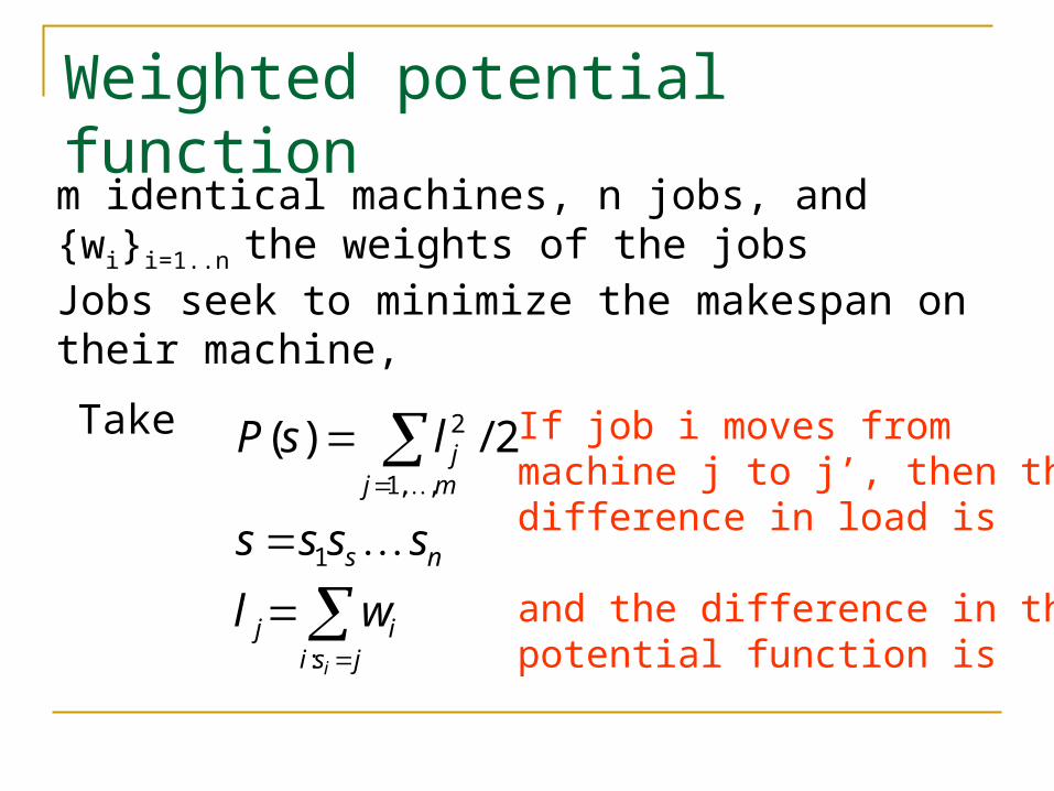
m identical machines, n jobs, and {wi}i=1..n the weights of the jobsJobs seek to minimize the makespan on their machine,

Take

jsiij

ns

mjj

i

wl

ssss

lsP

:

1

,,1

2 2/)(

If job i moves from machine j to j’, then thedifference in load is

and the difference in the potential function is

Weighted potential function (example)

jsiij

ns

mjj

i

wl

ssss

lsP

:

1

,,1

2 2/)(

m identical machines, {wi}i=1..n job weights

If job i moves from machine j to j’, then the difference in load is

ijji

iijiij

jjjj

ijjjj

ijj

ijj

wllw

wwlwwl

llllsPsP

wllll

wll

wll

'

22'

22'

22'

''

''

2/22

2

'')()'(

'

'

'

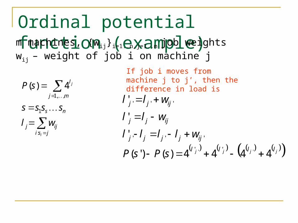
Ordinal potential function (example)

jsiijj

ns

mj

l

i

j

wl

ssss

sP

:

1

,,1

4)(

m machines, {wij}i=1..n,j=1..m job weightswij – weight of job i on machine j

If job i moves from machine j to j’, then the difference in load is

jjjj llll

ijjjjj

ijjj

ijjj

sPsP

wllll

wll

wll

4444)()'(

'

'

'

'' ''

'''

'''

(Exact) potential function

(1,1) (9,0)

(0,9) (6,6)PD =

4 3

3 0P4 =

u1(C,C) – u1(D,C) = P4(C,C) – P4(D,C)

u2(D,C) – u2(D,D) = P4(D,C) – P4(D,D)

C

C

D

D

u1(C,D) – u1(D,D) = P4(C,D) – P4(D,D)

u2(C,C) – u2(C,D) = P4(C,C) – P4(C,D)

P4 is a potential function for PD game

A function P (from S to R) is an (exact) PF for a game G if it is a w-potential function for G with w i = 1 for every i

Generalized ordinal potential function

(1,0) (2,0)

(2,0) (0,1)G’’ =

0 3

1 2P5 =

P5(A,B) – P5(A,A) > 0 implies that u1(A,B) – u1(A,A) > 0 but not that u2(A,B) – u2(A,A) > 0

A function P (from S to R) is an GOPF for a game G if for every player i ui(s-i, x) - ui(s-i, z) > 0 implies P(s-i, x) - P(s-i, z) > 0

for every x, z in Si and for every s-i in S-i

P5 is a generalized ordinal potential function for the game G’’

P5 is not an ordinal potential function for the game G’’

A

A

B

B

Potential games

A game that admits an OPF is called an ordinal potential game

A game that admits a weighted PF is called a weighted potential game

A game that admits an exact PF is called a potential game

In such games a Nash equilibrium is a local maximum for the potential

Equilibria in Potential Games

Thm (MS96) Let G be an ordinal potential game (P is an OPF). A strategy profile s in S is a pure equilibrium point for G iff for every player i it holds

P(s) ≥ P(s-i, x) for every x in Si

Therefore, if P has maximal value in S, then G has a pure Nash equilibrium.

Corollary Every finite OP game has a pure Nash equilibrium.

Nash equilibrium

P4 maximal value

An example

(1,1) (9,0)

(0,9) (6,6)PD =

C

C

D

D

4 3

3 0P4 =

(4,4) (3,3)

(3,3) (0,0)PD(P4) =

C

C

D

D

Thm (MS96)

FIP: an important property

A path in S is a sequence of states s.t. between every consecutive pair of states there is only one deviator

A path is an improvement path w.r.t. G if each deviator has a strict advantage

ui(sk) > ui(sk-1) G has the FIP if every improvement path is finite Clearly if G has the FIP then G has at least one pure

equilibrium Every improvement path terminates in an equilibrium point

FIP: an important property (2)Lemma Every finite OP game has the FIP.

The converse is true?

Lemma Let G be a finite game. Then, G has the FIP iff G has a generalized ordinal potential function.

(1,0) (2,0)

(2,0) (0,1)G’’ =

A

A

B

B• G’’ has the FIP ((B,A) is an equilibrium)

• any OPF must satisfies the following impossible relations:

P(A,A) < P(B,A) < P(B,B) < P(A,B) = P(A,A)

“No”

FIP: an important property (3)

Lemma Let G be a finite game. Then, G has the FIP iff G has a generalized ordinal potential function.Proof: Consider the graph of strict improvement moves. Give v the potential function value = the length of the longest path to a sink

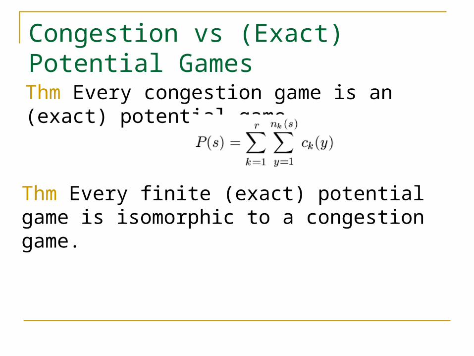
Congestion vs (Exact) Potential GamesThm Every congestion game is an (exact) potential game.

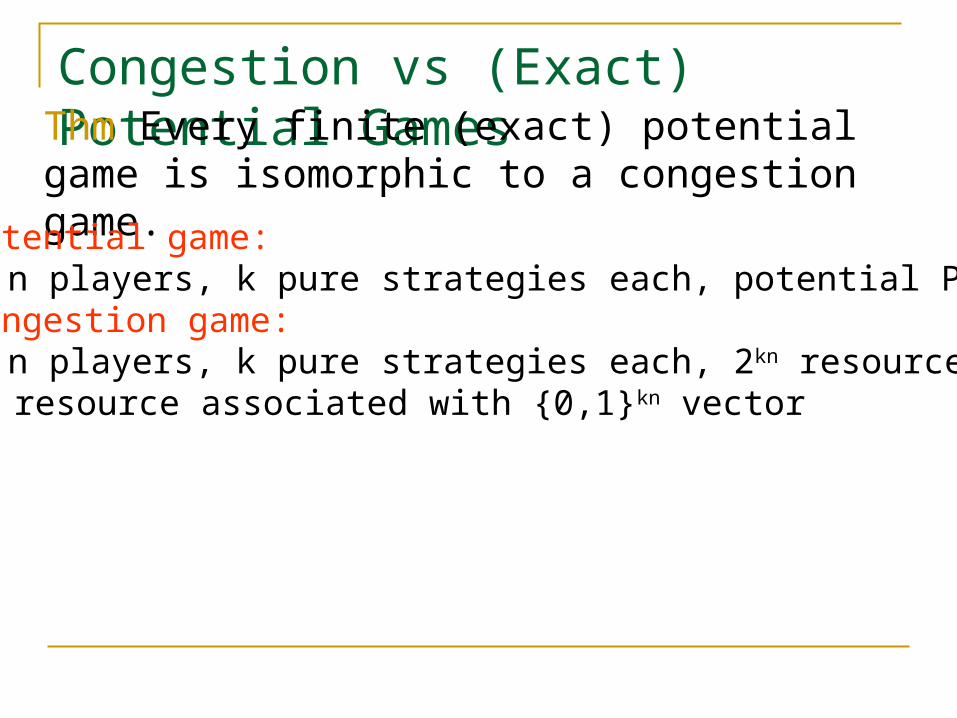
Thm Every finite (exact) potential game is isomorphic to a congestion game.

Congestion vs (Exact) Potential GamesThm Every finite (exact) potential game is

isomorphic to a congestion game.

• Potential game:• n players, k pure strategies each, potential P

• Congestion game:• n players, k pure strategies each, 2kn resources

resource associated with {0,1}kn vector

Congestion vs (Exact) Potential GamesThm Every finite (exact) potential game is

isomorphic to a congestion game.

•Congestion game:player 1 ≤ i ≤n plays pure strategy 0 ≤ q ≤ k-1:uses all resources rb where bit bik+q = 1 (2kn-1 res.)For every strategy vector s (for both games)b(s) where b(s)ik+q = 1 iff player i uses q in sFor n agents, the cost of rb(s) is P(s), for less agents the cost is 0For agent i, let b’ be such that b’jk+q= 0 if user j≠i uses strategy q, 1 otherwise. Cost of resource rb’ with one user ui(s)-P(s)

Final project part 1Improve the construction (use less resources)Why?

Computing NE in congestion games Sometimes easy (polytime) – symmetric

network congestion games Sometimes hard (PLS complete) – general

congestion games, symmetric congestion games, general network congestion games

Symmetric network congestion games (easy) Graph G=(V,E), source vertex v, sink t n players need to find a path from v to t. Congestion on edge e is given by c(e,k)

where k is the number of players using the edge (c ≥ 0)

Cost to player is sum of costs of edges player uses.

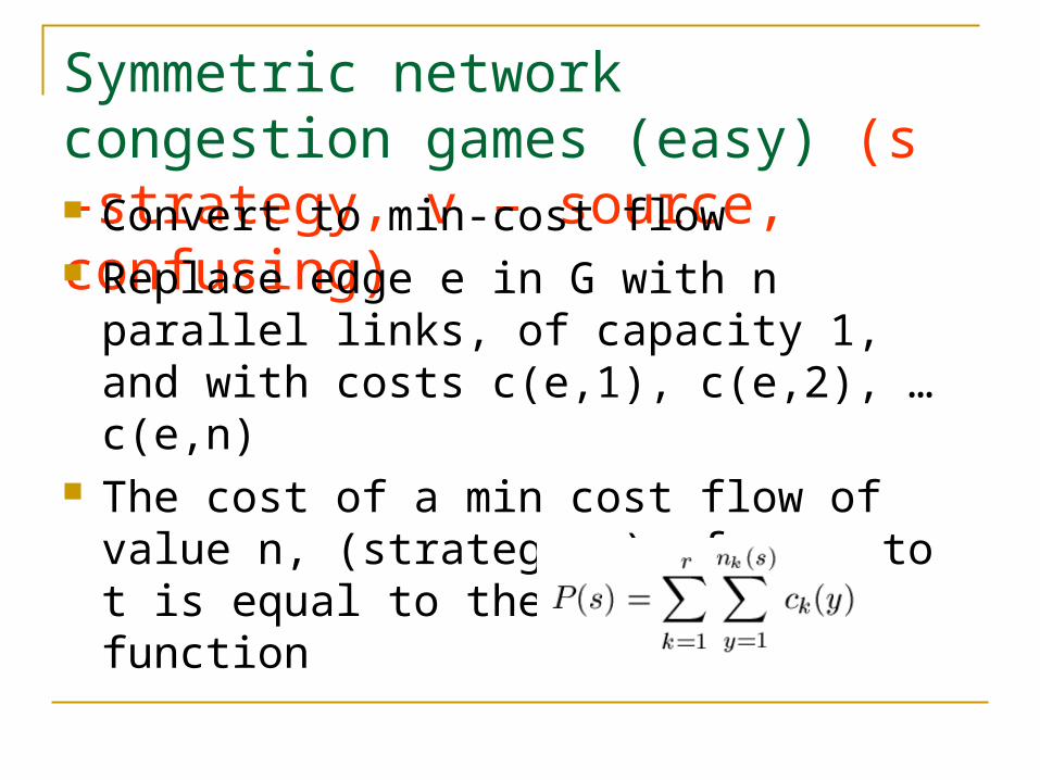
Symmetric network congestion games (easy) (s –strategy, v – source, confusing) Convert to min-cost flow Replace edge e in G with n parallel links, of

capacity 1, and with costs c(e,1), c(e,2), … c(e,n)

The cost of a min cost flow of value n, (strategy s), from v to t is equal to the potential function

Hardness results: Total Search

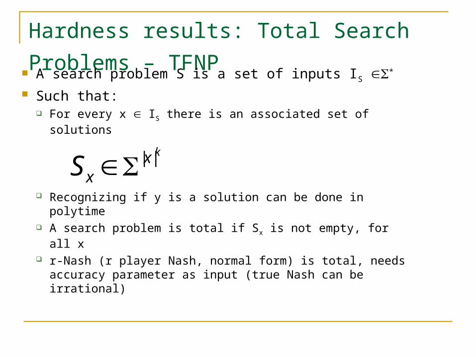
Problems – TFNP A search problem S is a set of inputs IS *

Such that: For every x IS there is an associated set of solutions

Recognizing if y is a solution can be done in polytime A search problem is total if Sx is not empty, for all x r-Nash (r player Nash, normal form) is total, needs

accuracy parameter as input (true Nash can be irrational)

kxxS

||

Total Search Problems – TFNP A search problem S is a set of inputs IS *

Such that: For every x IS there is an associated set of solutions

Recognizing if y is a solution can be done in polytime A search problem is total if Sx is not empty, for all x r-Nash (r player Nash, normal form) is total, needs

accuracy parameter as input (true Nash can be irrational)

kxxS

||

Subclasses of TFNP – PPAD and PLS PPAD: Polynomial Parity Argument, Directed Version (or just

that Papadimitriou has two p’s). End of Line problem:

n input bit circuits P and S (predecessor and successor) S(00…0) ≠ 00….0, P(00…0)=00…0 Find the end of the line (S(x)=x) or a loop (P(S(x))=x.

PPAD – class of total search problems reducible to “end of line”.

In particular – includes Brower Fixed point (discrete version) PPAD complete – natural notion. Brower is complete, 2 Player Nash is also complete. We saw how to use Brower to solve Nash, other direction also

works (major recent result – we will return to it when I understand it).

Subclasses of TFNP – PPAD and PLS PLS: Polynomial Local Search

A local search problem P belongs to PLS if:

For every instance I, a polytime algorithm A computes an initial feasible solution

A polytime algorithm B that computes, for every instance I and every feasible solution S, the objective function value c(S)

A polytime algorithm C that determines if S is locally optimal for instance I, and if not gives a better solution in the neighborhood of I

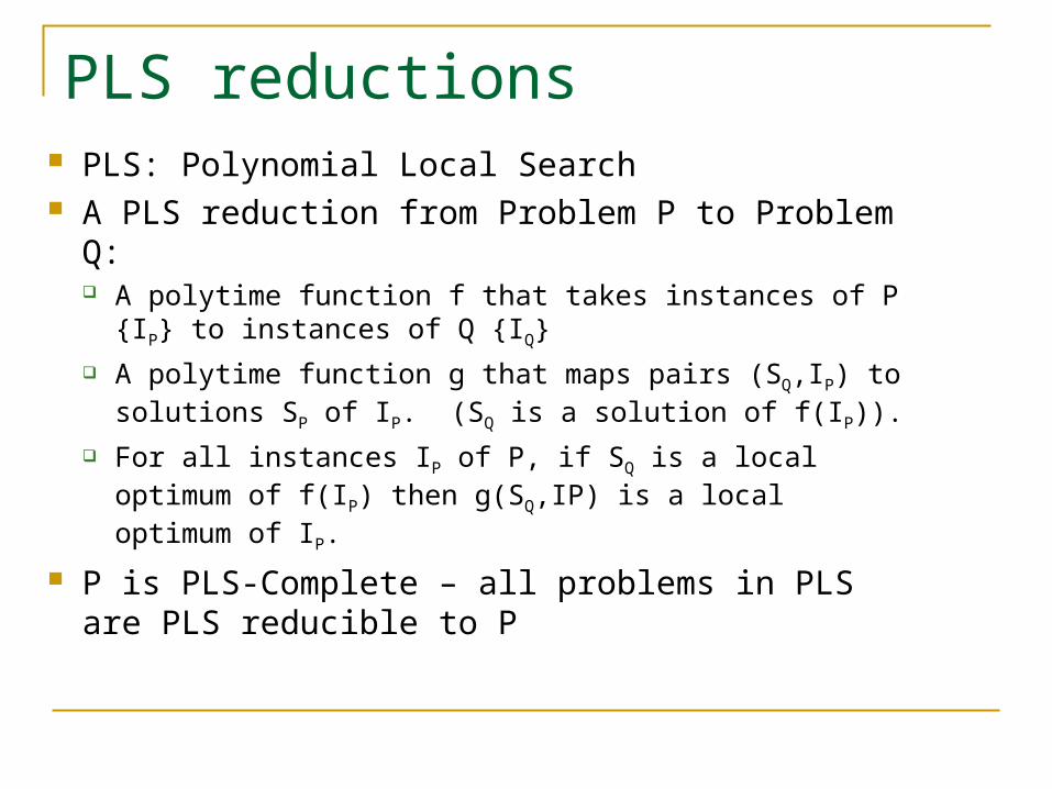
PLS reductions PLS: Polynomial Local Search A PLS reduction from Problem P to Problem Q:

A polytime function f that takes instances of P {IP} to instances of Q {IQ}

A polytime function g that maps pairs (SQ,IP) to solutions SP of IP. (SQ is a solution of f(IP)).

For all instances IP of P, if SQ is a local optimum of f(IP) then g(SQ,IP) is a local optimum of IP.

P is PLS-Complete – all problems in PLS are PLS reducible to P

PLS Complete problem – max cut (political party game)

Undirected graph G, weights on edges Find a partition of the vertices so that the sum of

the weights of edges crossing the cut is maximized (minimize disagreements within the party, high weight – high disagreement)

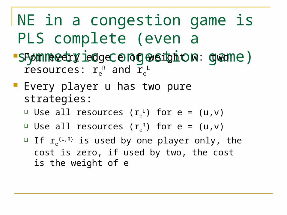
NE in a congestion game is PLS complete (even a symmetric congestion game) For every edge e of weight w: two resources: re

R and re

L

Every player u has two pure strategies: Use all resources (re

L) for e = (u,v)

Use all resources (reR) for e = (u,v)

If re{L,R} is used by one player only, the cost is zero, if

used by two, the cost is the weight of e