confidence intervals for two proportions - ncss.com€¦ · a background of the comparison of two...

PASS Sample Size Software NCSS.com

216-1 © NCSS, LLC. All Rights Reserved.

Chapter 216

Confidence Intervals for Two Proportions Introduction This routine calculates the group sample sizes necessary to achieve a specified interval width of the difference, ratio, or odds ratio of two independent proportions.

Caution: These procedures assume that the proportions obtained from future samples will be the same as the proportions that are specified. If the sample proportions are different from those specified when running these procedures, the interval width may be narrower or wider than specified.

Four Procedures Documented Here There are four procedures in the menus described in this chapter. These procedures are very similar except for the type of parameterization. The parameterization can be in terms of proportions, differences in proportions, ratios of proportions, and odds ratios.

Technical Details A background of the comparison of two proportions is given, followed by details of the confidence interval methods available in this procedure.

Comparing Two Proportions Suppose you have two populations from which dichotomous (binary) responses will be recorded. The probability (or risk) of obtaining the event of interest in population 1 (the treatment group) is 1p and in population 2 (the control group) is 2p . The corresponding failure proportions are given by 11 1 pq −= and 22 1 pq −= .

The assumption is made that the responses from each group follow a binomial distribution. This means that the event probability pi is the same for all subjects within a population and that the responses from one subject to the next are independent of one another.

Random samples of m and n individuals are obtained from these two populations. The data from these samples can be displayed in a 2-by-2 contingency table as follows

Success Failure Total Population 1 a c m

Population 2 b d n

Totals s f N

http://www.ncss.com/

PASS Sample Size Software NCSS.com Confidence Intervals for Two Proportions


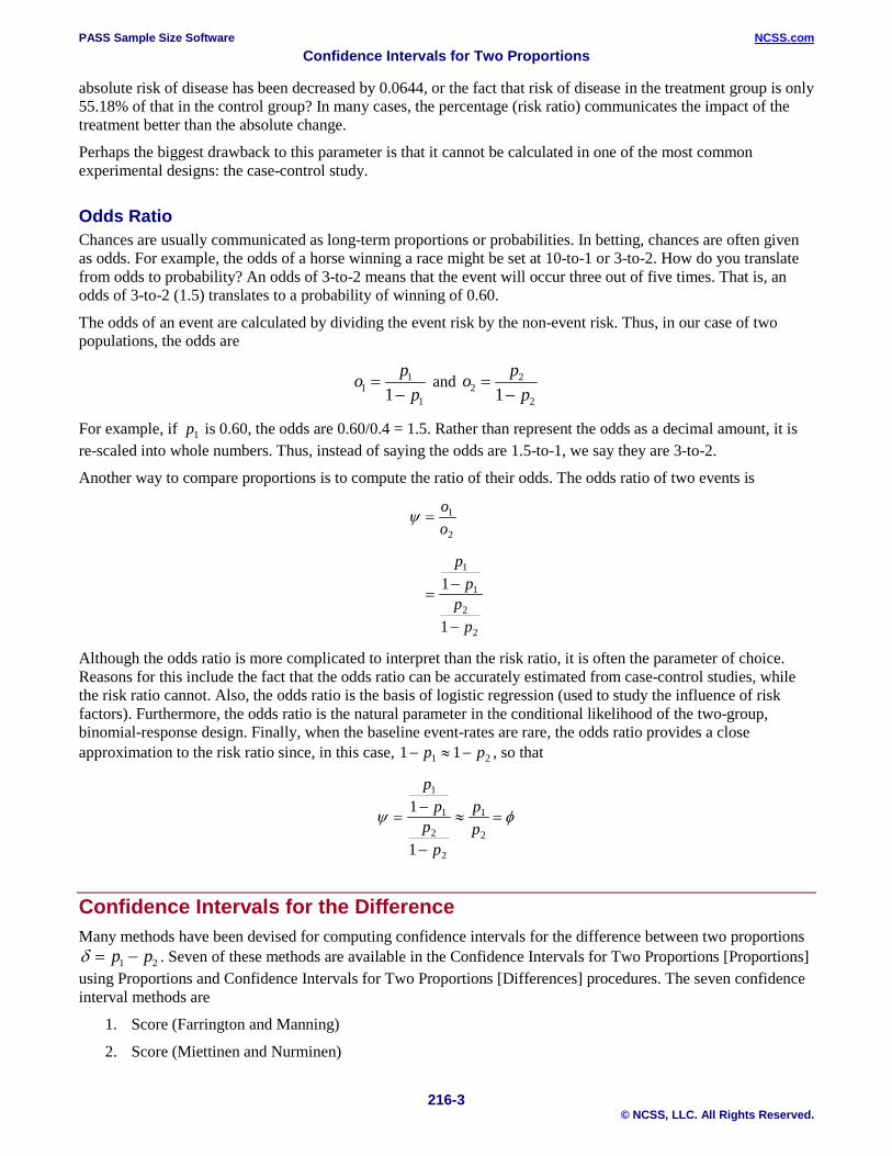
The following alternative notation is sometimes used:

Success Failure Total Population 1 x11 x12 n1

Population 2 x21 x22 n2

Totals m1 m2 N

The binomial proportions 1p and p2 are estimated from these data using the formulae

and p bn

xn2

21

2

= =

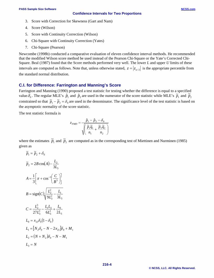
When analyzing studies such as these, you usually want to compare the two binomial probabilities 1p and 2p . The most direct methods of comparing these quantities are to calculate their difference or their ratio. If the binomial probability is expressed in terms of odds rather than probability, another measure is the odds ratio. Mathematically, these comparison parameters are

Parameter Computation

Difference 21 pp −=δ

Risk Ratio 21 / pp=φ

Odds Ratio 12

21

22

11

//

qpqp

qpqp

==ψ

The choice of which of these measures is used might at seem arbitrary, but it is important. Not only is their interpretation different, but, for small sample sizes, the coverage probabilities may be different.

Difference The (risk) difference 21 pp −=δ is perhaps the most direct method of comparison between the two event probabilities. This parameter is easy to interpret and communicate. It gives the absolute impact of the treatment. However, there are subtle difficulties that can arise with its interpretation.

One interpretation difficulty occurs when the event of interest is rare. If a difference of 0.001 were reported for an event with a baseline probability of 0.40, we would probability dismiss this as being of little importance. That is, there usually little interest in a treatment that decreases the probability from 0.400 to 0.399. However, if the baseline probably of a disease was 0.002 and 0.001 was the decrease in the disease probability, this would represent a reduction of 50%. Thus we see that interpretation depends on the baseline probability of the event.

A similar situation occurs when the amount of possible difference is considered. Consider two events, one with a baseline event rate of 0.40 and the other with a rate of 0.02. What is the maximum decrease that can occur? Obviously, the first event rate can be decreased by an absolute amount of 0.40 which the second can only be decreased by a maximum of 0.02.

So, although creating the simple difference is a useful method of comparison, care must be taken that it fits the situation.

Ratio The (risk) ratio 21 / pp=φ gives the relative change in the disease risk due to the application of the treatment. This parameter is also direct and easy to interpret. To compare this with the difference, consider a treatment that reduces the risk of disease for 0.1437 to 0.0793. Which single number is most enlightening, the fact that the

p am

xn111

1

= =




absolute risk of disease has been decreased by 0.0644, or the fact that risk of disease in the treatment group is only 55.18% of that in the control group? In many cases, the percentage (risk ratio) communicates the impact of the treatment better than the absolute change.

Perhaps the biggest drawback to this parameter is that it cannot be calculated in one of the most common experimental designs: the case-control study.

Odds Ratio Chances are usually communicated as long-term proportions or probabilities. In betting, chances are often given as odds. For example, the odds of a horse winning a race might be set at 10-to-1 or 3-to-2. How do you translate from odds to probability? An odds of 3-to-2 means that the event will occur three out of five times. That is, an odds of 3-to-2 (1.5) translates to a probability of winning of 0.60.

The odds of an event are calculated by dividing the event risk by the non-event risk. Thus, in our case of two populations, the odds are

o pp1

1

11=

− and o p

p22

21=

−

For example, if 1p is 0.60, the odds are 0.60/0.4 = 1.5. Rather than represent the odds as a decimal amount, it is re-scaled into whole numbers. Thus, instead of saying the odds are 1.5-to-1, we say they are 3-to-2.

Another way to compare proportions is to compute the ratio of their odds. The odds ratio of two events is

2

2

1

1

2

1

1

1

pp

pp

oo

−

−=

=ψ

Although the odds ratio is more complicated to interpret than the risk ratio, it is often the parameter of choice. Reasons for this include the fact that the odds ratio can be accurately estimated from case-control studies, while the risk ratio cannot. Also, the odds ratio is the basis of logistic regression (used to study the influence of risk factors). Furthermore, the odds ratio is the natural parameter in the conditional likelihood of the two-group, binomial-response design. Finally, when the baseline event-rates are rare, the odds ratio provides a close approximation to the risk ratio since, in this case, 21 11 pp −≈− , so that

φψ =≈

−

−=

2

1

2

2

1

1

1

1pp

pp

pp

Confidence Intervals for the Difference Many methods have been devised for computing confidence intervals for the difference between two proportions δ = −p p1 2 . Seven of these methods are available in the Confidence Intervals for Two Proportions [Proportions] using Proportions and Confidence Intervals for Two Proportions [Differences] procedures. The seven confidence interval methods are

1. Score (Farrington and Manning)

2. Score (Miettinen and Nurminen)




3. Score with Correction for Skewness (Gart and Nam)

4. Score (Wilson)

5. Score with Continuity Correction (Wilson)

6. Chi-Square with Continuity Correction (Yates)

7. Chi-Square (Pearson)

Newcombe (1998b) conducted a comparative evaluation of eleven confidence interval methods. He recommended that the modified Wilson score method be used instead of the Pearson Chi-Square or the Yate’s Corrected Chi-Square. Beal (1987) found that the Score methods performed very well. The lower L and upper U limits of these intervals are computed as follows. Note that, unless otherwise stated, z z= α / 2 is the appropriate percentile from the standard normal distribution.

C.I. for Difference: Farrington and Manning’s Score Farrington and Manning (1990) proposed a test statistic for testing whether the difference is equal to a specified valueδ0 . The regular MLE’s p1 and p2 are used in the numerator of the score statistic while MLE’s 1

~p and ~p2 constrained so that 021

~~ δ=− pp are used in the denominator. The significance level of the test statistic is based on the asymptotic normality of the score statistic.

The test statistic formula is

+

−−=

2

22

1

11

021

~~~~ˆˆ

nqp

nqp

ppzFMDδ

where the estimates ~p1 and ~p2 are computed as in the corresponding test of Miettinen and Nurminen (1985) given as

021~~ δ+= pp

( )3

22 3

cos2~LLABp −=

+= −

31cos

31

BCA π

( )3

123

22

39sign

LL

LLCB −=

3

023

2133

32

2627 LL

LLL

LLC +−=

( )00210 1 δδ −= xL

[ ] 1021021 2 MxNNL +−−= δδ

( ) 1022 MNNNL −−+= δ

NL =3




Farrington and Manning (1990) proposed inverting their score test to find the confidence interval. The lower limit is found by solving

2/αzzFMD =

and the upper limit is the solution of

2/αzzFMD −=

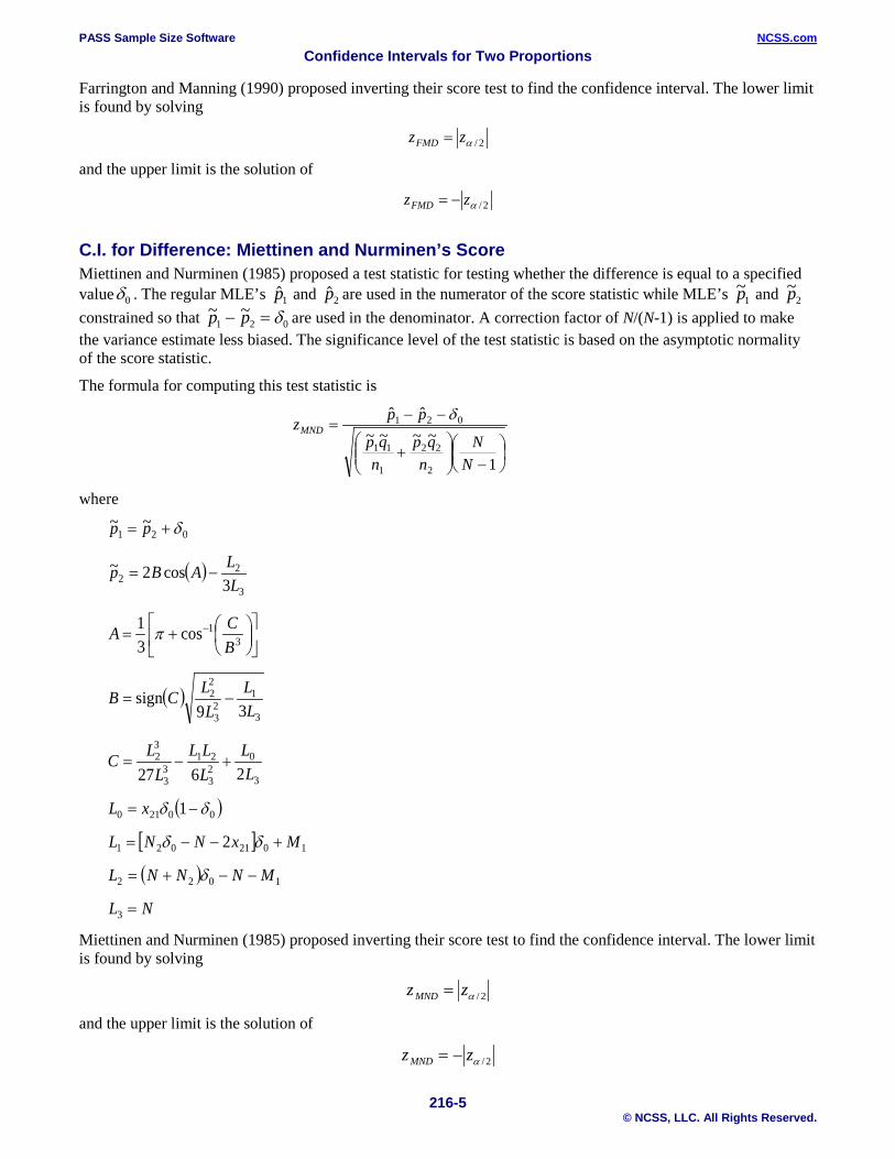
C.I. for Difference: Miettinen and Nurminen’s Score Miettinen and Nurminen (1985) proposed a test statistic for testing whether the difference is equal to a specified valueδ0 . The regular MLE’s p1 and p2 are used in the numerator of the score statistic while MLE’s ~p1 and ~p2 constrained so that ~ ~p p1 2 0− = δ are used in the denominator. A correction factor of N/(N-1) is applied to make the variance estimate less biased. The significance level of the test statistic is based on the asymptotic normality of the score statistic.

The formula for computing this test statistic is

−

+

−−=

1

~~~~ˆˆ

2

22

1

11

021

NN

nqp

nqp

ppzMNDδ

where

021~~ δ+= pp

( )3

22 3

cos2~LLABp −=

+= −

31cos

31

BCA π

( )3

123

22

39sign

LL

LLCB −=

3

023

2133

32

2627 LL

LLL

LLC +−=

( )00210 1 δδ −= xL

[ ] 1021021 2 MxNNL +−−= δδ

( ) 1022 MNNNL −−+= δ

NL =3

Miettinen and Nurminen (1985) proposed inverting their score test to find the confidence interval. The lower limit is found by solving

z zMND = α / 2


z zMND = − α / 2




C.I. for Difference: Gart and Nam’s Score Gart and Nam (1990) page 638 proposed a modification to the Farrington and Manning (1990) difference test that corrected for skewness. Let ( )zFM δ stand for the Farrington and Manning difference test statistic described above. The skewness corrected test statistic zGN is the appropriate solution to the quadratic equation

( ) ( ) ( )( )− + − + + =~ ~γ δ γz z zGND GND FMD2 1 0

where

( ) ( ) ( )

−−

−= 2

2

222221

11112/3 ~~~~~~~~

6

~~

npqqp

npqqpV δγ

Gart and Nam (1988) proposed inverting their score test to find the confidence interval. The lower limit is found by solving

2/αzzGND =


2/αzzGND −=

C.I. for Difference: Wilson’s Score as Modified by Newcombe (with and without Continuity Correction) For details, see Newcombe (1998b), page 876.

BppL −−= 21 ˆˆ

CppU +−= 21 ˆˆ

where

( ) ( )n

uum

llzB 2211 11 −+

−=

( ) ( )n

llm

uuzC 2211 11 −+

−=

and l1 and u1 are the roots of

( ) 01ˆ 1111 =

−−−

mppzpp

and l2 and u2 are the roots of

( ) 01ˆ 2222 =

−−−

nppzpp




C.I. for Difference: Yate’s Chi-Square with Continuity Correction For details, see Newcombe (1998b), page 875.

++

−

+−

−−=nmn

ppm

ppzppL 1121)ˆ1(ˆ)ˆ1(ˆˆˆ 2211

21

++

−

+−

+−=nmn

ppm

ppzppU 1121)ˆ1(ˆ)ˆ1(ˆˆˆ 2211

21

C.I. for Difference: Pearson’s Chi-Square For details, see Newcombe (1998b), page 875.

−

+−

−−=n

ppm

ppzppL )ˆ1(ˆ)ˆ1(ˆˆˆ 221121

−

+−

+−=n

ppm

ppzppU )ˆ1(ˆ)ˆ1(ˆˆˆ 221121

For each of the seven methods, one-sided intervals may be obtained by replacing α/2 by α.

For two-sided intervals, the distance from the difference in sample proportions to each of the limits may be different. Thus, instead of specifying the distance to the limits we specify the width of the interval, W.

The basic equation for determining sample size for a two-sided interval when W has been specified is

LUW −=

For one-sided intervals, the distance from the variance ratio to limit, D, is specified.

The basic equation for determining sample size for a one-sided upper limit when D has been specified is

( )21 ppUD ˆˆ −−=

The basic equation for determining sample size for a one-sided lower limit when D has been specified is

( ) LppD −−= 21 ˆˆ

Each of these equations can be solved for any of the unknown quantities in terms of the others.

Confidence Intervals for the Ratio (Relative Risk) Many methods have been devised for computing confidence intervals for the ratio (relative risk) of two proportions 21 / pp=φ . Six of these methods are available in the Confidence Intervals for Two Proportions [Ratios] procedure. The six confidence interval methods are



3. Score with Correction for Skewness (Gart and Nam)

4. Logarithm (Katz)

5. Logarithm + 1/2 (Walter)

6. Fleiss




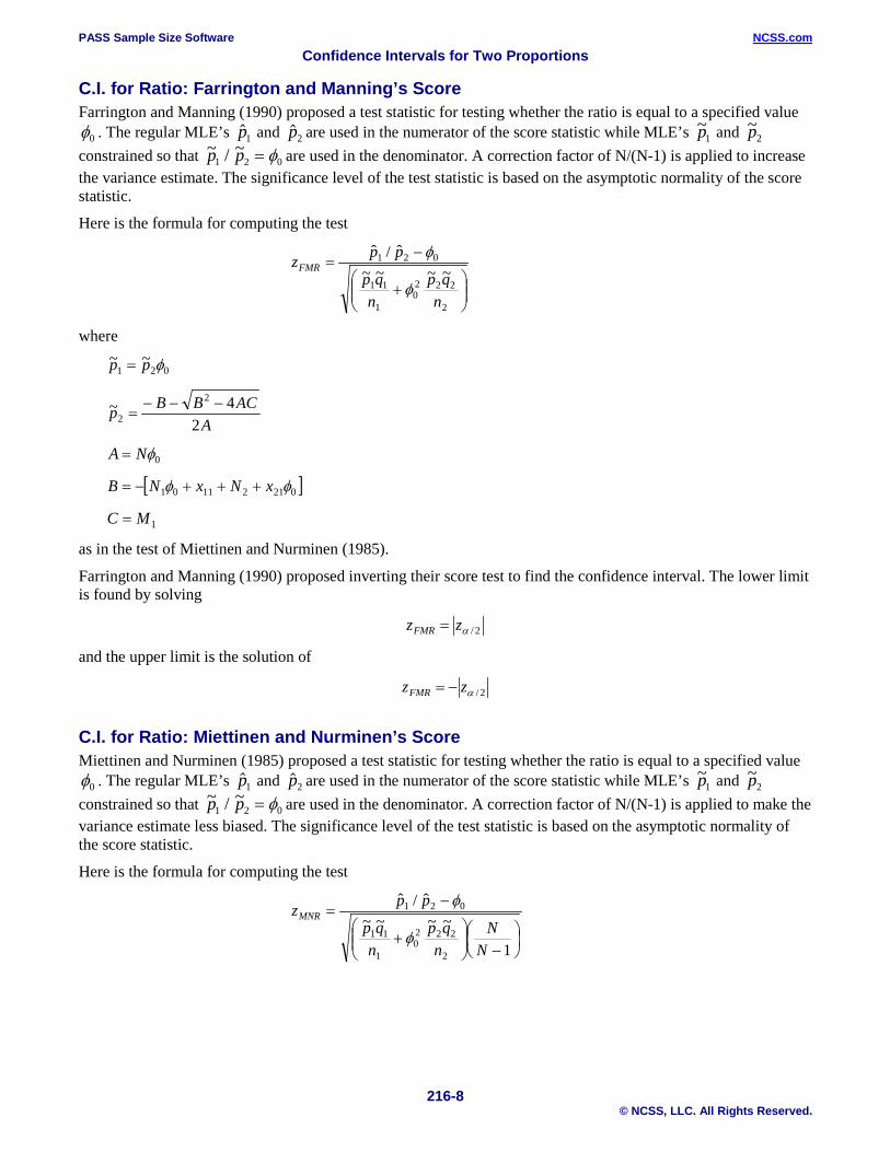
C.I. for Ratio: Farrington and Manning’s Score Farrington and Manning (1990) proposed a test statistic for testing whether the ratio is equal to a specified valueφ0 . The regular MLE’s p1 and p2 are used in the numerator of the score statistic while MLE’s ~p1 and ~p2 constrained so that ~ / ~p p1 2 0= φ are used in the denominator. A correction factor of N/(N-1) is applied to increase the variance estimate. The significance level of the test statistic is based on the asymptotic normality of the score statistic.

Here is the formula for computing the test

+

−=

2

2220

1

11

021

~~~~ˆ/ˆ

nqp

nqp

ppzFMR

φ

φ

where

021~~ φpp =

AACBBp

24~

2

2−−−

=

0φNA =

[ ]02121101 φφ xNxNB +++−=

1MC =

as in the test of Miettinen and Nurminen (1985).


2/αzzFMR =


2/αzzFMR −=

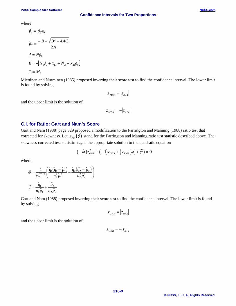
C.I. for Ratio: Miettinen and Nurminen’s Score Miettinen and Nurminen (1985) proposed a test statistic for testing whether the ratio is equal to a specified valueφ0 . The regular MLE’s p1 and p2 are used in the numerator of the score statistic while MLE’s ~p1 and ~p2 constrained so that ~ / ~p p1 2 0= φ are used in the denominator. A correction factor of N/(N-1) is applied to make the variance estimate less biased. The significance level of the test statistic is based on the asymptotic normality of the score statistic.

Here is the formula for computing the test

−

+

−=

1

~~~~ˆ/ˆ

2

2220

1

11

021

NN

nqp

nqp

ppzMNR

φ

φ




where

021~~ φpp =

AACBBp

24~

2

2−−−

=

0φNA =

[ ]02121101 φφ xNxNB +++−=

1MC =


z zMNR = α / 2


z zMNR = − α / 2

C.I. for Ratio: Gart and Nam’s Score Gart and Nam (1988) page 329 proposed a modification to the Farrington and Manning (1988) ratio test that corrected for skewness. Let ( )zFM φ stand for the Farrington and Manning ratio test statistic described above. The skewness corrected test statistic zGN is the appropriate solution to the quadratic equation

( ) ( ) ( )( )− + − + + =~ ~ϕ φ ϕz z zGNR GNR FMR2 1 0

where

( ) ( )

−−

−= 2

222

22221

21

1112/3 ~

~~~~

~~~~61~

pnpqq

pnpqq

uϕ

22

2

11

1~

~~

~~pn

qpn

qu +=

Gart and Nam (1988) proposed inverting their score test to find the confidence interval. The lower limit is found by solving

z zGNR = α / 2


z zGNR = − α / 2




C.I. for Ratio: Logarithm (Katz) This was one of the first methods proposed for computing confidence intervals for risk ratios.

For details, see Gart and Nam (1988), page 324.

+−=

2

2

1

1

ˆˆ

ˆˆ

expˆpnq

pnqzL φ

+=

2

2

1

1

ˆˆ

ˆˆ

expˆpnq

pnqzU φ

where

2

1

ˆˆˆpp

=φ

C.I. for Ratio: Logarithm (Walters) For details, see Gart and Nam (1988), page 324.

( )uzL ˆexpˆ −= φ

( )uzU ˆexpφ̂=

where

++

−

++

=2121

2121

lnlnexpˆnb

ma

φ

ua m b n

=+

−+

++

−+

1 1 1 112

12

12

12

22~1~ pq −=

1

2

2

1

12~~

~~ −

+=

pnq

pmqV φ

21~~ pp φ=

11~1~ pq −=

22~1~ pq −=

( )( )

( )( )

−−

−= 2

2

2222

1

1112/33 ~

~~~~

~~~~pn

pqqpm

pqqvµ

1

2

2

1

1~~

~~ −

+=

pnq

pmqv




C.I. for Odds Ratio and Relative Risk: Iterated Method of Fleiss Fleiss (1981) presents an improved confidence interval for the odds ratio and relative risk. This method forms the confidence interval as all those value of the odds ratio which would not be rejected by a chi-square hypothesis test. Fleiss gives the following details about how to construct this confidence interval. To compute the lower limit, do the following.

1. For a trial value of ψ , compute the quantities X, Y, W, F, U, and V using the formulas

( ) ( )snsmX −++=ψ

( )142 −−= ψψmsXY

( )12 −−

=ψ

YXA

AsB −=

AmC −=

AmfD +−=

DCBAW 1111

+++=

( ) 22/

221

αzWAaF −−−=

( )( ) ( )[ ]

−−+

−−−

−= 1221

121

2 ψψψ

mssmXY

nYT

22221111

DACBU −−+=

( ) ( )[ ]212

21 2 −−−−−= AaWUAaTV

Finally, use the updating equation below to calculate a new value for the odds ratio using the updating equation

( ) ( )VFkk −=+ ψψ 1

2. Continue iterating until the value of F is arbitrarily close to zero.

The upper limit is found by substituting + 12 for − 1

2 in the formulas for F and V.

Confidence limits for the relative risk can be calculated using the expected counts A, B, C, and D from the last iteration of the above procedure. The lower limit of the relative risk

mBnA

lower

lowerlower =φ

mBnA

upper

upperupper =φ




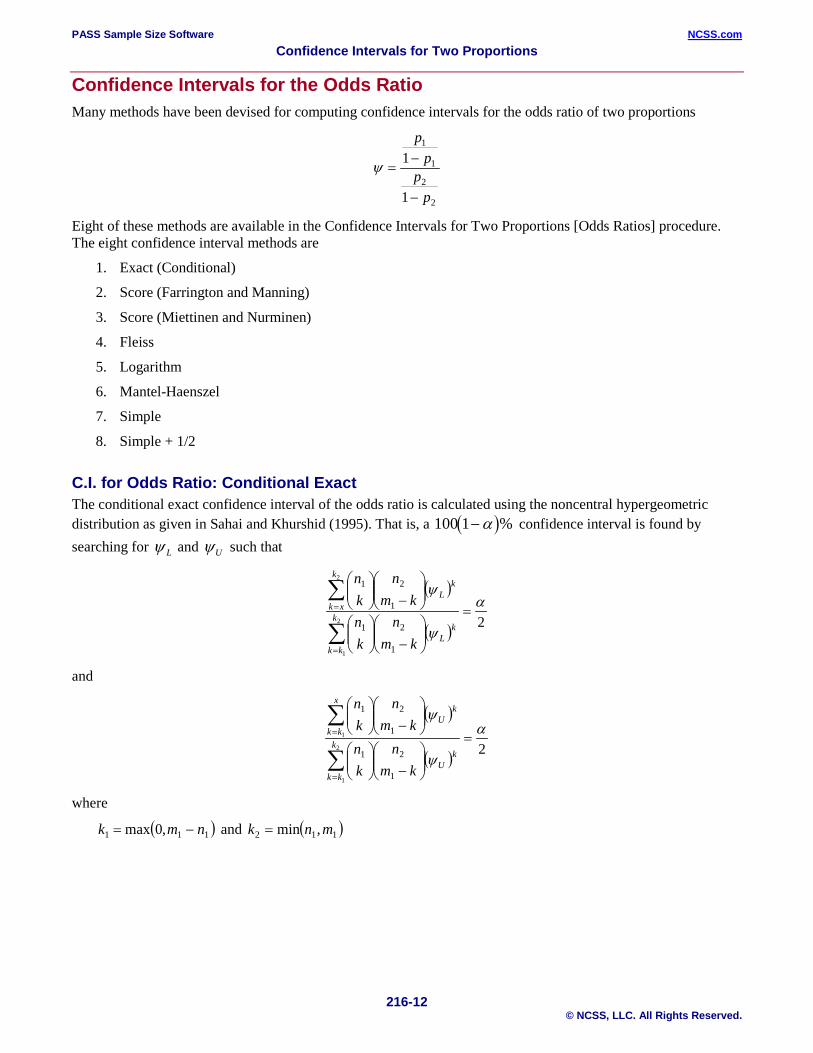
Confidence Intervals for the Odds Ratio Many methods have been devised for computing confidence intervals for the odds ratio of two proportions

2

2

1

1

1

1

pp

pp

−

−=ψ

Eight of these methods are available in the Confidence Intervals for Two Proportions [Odds Ratios] procedure. The eight confidence interval methods are

1. Exact (Conditional)



4. Fleiss

5. Logarithm

6. Mantel-Haenszel

7. Simple

8. Simple + 1/2

C.I. for Odds Ratio: Conditional Exact The conditional exact confidence interval of the odds ratio is calculated using the noncentral hypergeometric distribution as given in Sahai and Khurshid (1995). That is, a ( )100 1−α % confidence interval is found by searching for ψ L and ψU such that

( )

( ) 22

1

2

1

21

1

21

α

ψ

ψ=

−

−

∑

∑

=

=k

kk

kL

k

xk

kL

kmn

kn

kmn

kn

and

( )

( ) 22

1

1

1

21

1

21

α

ψ

ψ=

−

−

∑

∑

=

=k

kk

kU

x

kk

kU

kmn

kn

kmn

kn

where

( )111 ,0max nmk −= and ( )112 ,min mnk =




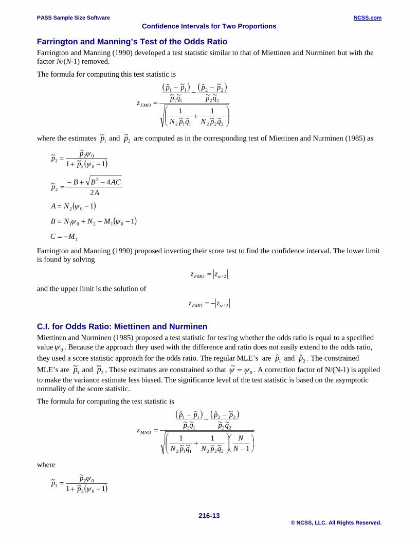
Farrington and Manning’s Test of the Odds Ratio Farrington and Manning (1990) developed a test statistic similar to that of Miettinen and Nurminen but with the factor N/(N-1) removed.

The formula for computing this test statistic is

( ) ( )

+

−−

−

=

222112

22

22

11

11

~~1

~~1

~~~ˆ

~~~ˆ

qpNqpN

qppp

qppp

zFMO

where the estimates ~p1 and ~p2 are computed as in the corresponding test of Miettinen and Nurminen (1985) as

( )1~1

~~02

021 −+=

ψψ

ppp

AACBBp

24~

2

2−+−

=

( )102 −= ψNA

( )101201 −−+= ψψ MNNB

1MC −=


2/αzzFMO =


2/αzzFMO −=

C.I. for Odds Ratio: Miettinen and Nurminen Miettinen and Nurminen (1985) proposed a test statistic for testing whether the odds ratio is equal to a specified valueψ 0 . Because the approach they used with the difference and ratio does not easily extend to the odds ratio, they used a score statistic approach for the odds ratio. The regular MLE’s are p1 and p2 . The constrained MLE’s are ~p1 and ~p2 , These estimates are constrained so that ~ψ ψ= 0 . A correction factor of N/(N-1) is applied to make the variance estimate less biased. The significance level of the test statistic is based on the asymptotic normality of the score statistic.

The formula for computing the test statistic is

( ) ( )

−

+

−−

−

=

1~~1

~~1

~~~ˆ

~~~ˆ

222112

22

22

11

11

NN

qpNqpN

qppp

qppp

zMNO

where

( )1~1

~~02

021 −+=

ψψ

ppp




AACBBp

24~

2

2−+−

=

( )102 −= ψNA

( )101201 −−+= ψψ MNNB

1MC −=


2/αzzMNO =


2/αzzMNO −=

C.I. for Odds Ratio: Iterated Method of Fleiss Fleiss (1981) presents an improve confidence interval for the odds ratio. This method forms the confidence interval as all those value of the odds ratio which would not be rejected by a chi-square hypothesis test. Fleiss gives the following details about how to construct this confidence interval. To compute the lower limit, do the following.

1. For a trial value of ψ , compute the quantities X, Y, W, F, U, and V using the formulas

( ) ( )snsmX −++=ψ

( )142 −−= ψψmsXY

( )12 −−

=ψ

YXA

AsB −=

AmC −=

AmfD +−=

DCBAW 1111

+++=

( ) 22/

221

αzWAaF −−−=

( )( ) ( )[ ]

−−+

−−−

−= 1221

121

..2 ψψψ

mssmXY

nYT

22221111

DACBU −−+=

( ) ( )[ ]212

21 2 −−−−−= AaWUAaTV




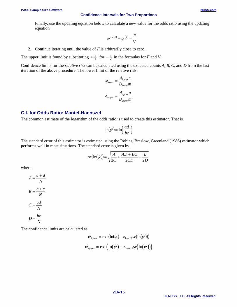
Finally, use the updating equation below to calculate a new value for the odds ratio using the updating equation

( ) ( )VFkk −=+ ψψ 1

2. Continue iterating until the value of F is arbitrarily close to zero.

The upper limit is found by substituting + 12 for − 1

2 in the formulas for F and V.

Confidence limits for the relative risk can be calculated using the expected counts A, B, C, and D from the last iteration of the above procedure. The lower limit of the relative risk

mBnA

lower

lowerlower =φ

mBnA

upper

upperupper =φ

C.I. for Odds Ratio: Mantel-Haenszel The common estimate of the logarithm of the odds ratio is used to create this estimator. That is

( )

=

bcadlnˆlnψ

The standard error of this estimator is estimated using the Robins, Breslow, Greenland (1986) estimator which performs well in most situations. The standard error is given by

( )( )DB

CDBCAD

CA

222ˆlnse +

++=ψ

where

NdaA +

=

NcbB +

=

NadC =

NbcD =

The confidence limits are calculated as

( ) ( )( )( )ψψψ α ˆlnˆlnexpˆ 2/1 sezlower −−=

( ) ( )( )( ) exp ln ln /ψ ψ ψαupper z se= + −1 2




C.I. for Odds Ratio: Simple, Simple + ½, and Logarithm The simple estimate of the odds ratio uses the formula

bcad

qpqp

=

=12

21

ˆˆˆˆ

ψ̂

The standard error of this estimator is estimated by

( )dcba

se 1111ˆˆ +++=ψψ

Problems occur if any one of the quantities a, b, c, or d are zero. To correct this problem, many authors recommend adding one-half to each cell count so that a zero cannot occur. Now, the formulas become

( )( )( )( )5.05.0

5.05.0ˆ++++

=′cbdaψ

and

( )5.0

15.0

15.0

15.0

1ˆˆ+

++

++

++

′=′dcba

se ψψ

The distribution of these direct estimates of the odds ratio do not converge to normality as fast as does their logarithm, so the logarithm of the odds ratio is used to form confidence intervals. The formula for the standard error of the log odds ratio is

( )ψ ′=′ ˆlnL

and

( )5.0

15.0

15.0

15.0

1+

++

++

++

=′dcba

Lse

A ( )%1100 α− confidence interval for the log odds ratio is formed using the standard normal distribution as follows

( )( )LsezLlower ′−′= − 2/1expˆ αψ

( )( )LsezLupper ′+′= − 2/1expˆ αψ

See Fleiss et al (2003) for more details.

Confidence Level The confidence level, 1 – α, has the following interpretation. If thousands of random samples of size n1 and n2 are drawn from populations 1 and 2, respectively, and a confidence interval for the true difference/ratio/odds ratio of proportions is calculated for each pair of samples, the proportion of those intervals that will include the true difference/ratio/odds ratio of proportions is 1 – α.




Procedure Options This section describes the options that are specific to this procedure. These are located on the Design tab. For more information about the options of other tabs, go to the Procedure Window chapter.

Design Tab (Common Options) This chapter covers four procedures, each of which has different options. This section documents options that are common to all four procedures. Following this section, the unique options for each procedure (proportions, differences, ratios, and odds ratios) will be documented.

Solve For

Solve For This option specifies the parameter to be solved for from the other parameters.

One-Sided or Two-Sided Interval

Interval Type Specify whether the interval to be used will be a two-sided confidence interval, an interval that has only an upper limit, or an interval that has only a lower limit.

Confidence

Confidence Level The confidence level, 1 – α, has the following interpretation. If thousands of random samples of size n1 and n2 are drawn from populations 1 and 2, respectively, and a confidence interval for the true difference/ratio/odds ratio of proportions is calculated for each pair of samples, the proportion of those intervals that will include the true difference/ratio/odds ratio of proportions is 1 – α.

Often, the values 0.95 or 0.99 are used. You can enter single values or a range of values such as 0.90, 0.95 or 0.90 to 0.99 by 0.01.

Sample Size (When Solving for Sample Size)

Group Allocation Select the option that describes the constraints on N1 or N2 or both.

The options are

• Equal (N1 = N2) This selection is used when you wish to have equal sample sizes in each group. Since you are solving for both sample sizes at once, no additional sample size parameters need to be entered.

• Enter N1, solve for N2 Select this option when you wish to fix N1 at some value (or values), and then solve only for N2. Please note that for some values of N1, there may not be a value of N2 that is large enough to obtain the desired power.

• Enter N2, solve for N1 Select this option when you wish to fix N2 at some value (or values), and then solve only for N1. Please note that for some values of N2, there may not be a value of N1 that is large enough to obtain the desired power.




• Enter R = N2/N1, solve for N1 and N2 For this choice, you set a value for the ratio of N2 to N1, and then PASS determines the needed N1 and N2, with this ratio, to obtain the desired power. An equivalent representation of the ratio, R, is

N2 = R * N1.

• Enter percentage in Group 1, solve for N1 and N2 For this choice, you set a value for the percentage of the total sample size that is in Group 1, and then PASS determines the needed N1 and N2 with this percentage to obtain the desired power.

N1 (Sample Size, Group 1) This option is displayed if Group Allocation = “Enter N1, solve for N2”

N1 is the number of items or individuals sampled from the Group 1 population.

N1 must be ≥ 2. You can enter a single value or a series of values.

N2 (Sample Size, Group 2) This option is displayed if Group Allocation = “Enter N2, solve for N1”



R (Group Sample Size Ratio) This option is displayed only if Group Allocation = “Enter R = N2/N1, solve for N1 and N2.”

R is the ratio of N2 to N1. That is,

R = N2 / N1.

Use this value to fix the ratio of N2 to N1 while solving for N1 and N2. Only sample size combinations with this ratio are considered.

N2 is related to N1 by the formula:

N2 = [R × N1],

where the value [Y] is the next integer ≥ Y.

For example, setting R = 2.0 results in a Group 2 sample size that is double the sample size in Group 1 (e.g., N1 = 10 and N2 = 20, or N1 = 50 and N2 = 100).

R must be greater than 0. If R < 1, then N2 will be less than N1; if R > 1, then N2 will be greater than N1. You can enter a single or a series of values.

Percent in Group 1 This option is displayed only if Group Allocation = “Enter percentage in Group 1, solve for N1 and N2.”

Use this value to fix the percentage of the total sample size allocated to Group 1 while solving for N1 and N2. Only sample size combinations with this Group 1 percentage are considered. Small variations from the specified percentage may occur due to the discrete nature of sample sizes.

The Percent in Group 1 must be greater than 0 and less than 100. You can enter a single or a series of values.




Sample Size (When Not Solving for Sample Size)

Group Allocation Select the option that describes how individuals in the study will be allocated to Group 1 and to Group 2.

The options are

• Equal (N1 = N2) This selection is used when you wish to have equal sample sizes in each group. A single per group sample size will be entered.

• Enter N1 and N2 individually This choice permits you to enter different values for N1 and N2.

• Enter N1 and R, where N2 = R * N1 Choose this option to specify a value (or values) for N1, and obtain N2 as a ratio (multiple) of N1.

• Enter total sample size and percentage in Group 1 Choose this option to specify a value (or values) for the total sample size (N), obtain N1 as a percentage of N, and then N2 as N - N1.

Sample Size Per Group This option is displayed only if Group Allocation = “Equal (N1 = N2).”

The Sample Size Per Group is the number of items or individuals sampled from each of the Group 1 and Group 2 populations. Since the sample sizes are the same in each group, this value is the value for N1, and also the value for N2.

The Sample Size Per Group must be ≥ 2. You can enter a single value or a series of values.

N1 (Sample Size, Group 1) This option is displayed if Group Allocation = “Enter N1 and N2 individually” or “Enter N1 and R, where N2 = R * N1.”



N2 (Sample Size, Group 2) This option is displayed only if Group Allocation = “Enter N1 and N2 individually.”



R (Group Sample Size Ratio) This option is displayed only if Group Allocation = “Enter N1 and R, where N2 = R * N1.”

R is the ratio of N2 to N1. That is,

R = N2/N1

Use this value to obtain N2 as a multiple (or proportion) of N1.

N2 is calculated from N1 using the formula:

N2=[R x N1],

where the value [Y] is the next integer ≥ Y.




For example, setting R = 2.0 results in a Group 2 sample size that is double the sample size in Group 1.

R must be greater than 0. If R < 1, then N2 will be less than N1; if R > 1, then N2 will be greater than N1. You can enter a single value or a series of values.

Total Sample Size (N) This option is displayed only if Group Allocation = “Enter total sample size and percentage in Group 1.”

This is the total sample size, or the sum of the two group sample sizes. This value, along with the percentage of the total sample size in Group 1, implicitly defines N1 and N2.

The total sample size must be greater than one, but practically, must be greater than 3, since each group sample size needs to be at least 2.

You can enter a single value or a series of values.

Percent in Group 1 This option is displayed only if Group Allocation = “Enter total sample size and percentage in Group 1.”

This value fixes the percentage of the total sample size allocated to Group 1. Small variations from the specified percentage may occur due to the discrete nature of sample sizes.

The Percent in Group 1 must be greater than 0 and less than 100. You can enter a single value or a series of values.

Design Tab (Proportions) This section documents options that are used when the parameterization is in terms of the values of the two sample proportions, P1 and P2. The corresponding procedure is Confidence Intervals for the Difference between Two Proportions using Proportions.

Confidence Interval Method

Confidence Interval Formula Specify the formula to be in used in calculation of confidence intervals.

• Score (Farrington & Manning) This formula is based on inverting Farrington and Manning's score test.

• Score (Miettinen & Nurminen) This formula is based on inverting Miettinen and Nurminen's score test.

• Score w/ Skewness (Gart & Nam) This formula is based on inverting Gart and Nam's score test, with a correction for skewness.

• Score (Wilson) This formula is based on the Wilson score method for a single proportion, without continuity correction.

• Score (Wilson C.C.) This formula is based on the Wilson score method for a single proportion, with continuity correction.

• Chi-Square C.C. (Yates) This is the commonly used simple asymptotic method, with continuity correction.




• Chi-Square (Pearson) This is the commonly used simple asymptotic method, without continuity correction.

Precision

Confidence Interval Width (Two-Sided) This is the distance from the lower confidence limit to the upper confidence limit.

You can enter a single value or a list of values. The value(s) must be greater than zero.

Distance from Diff to Limit (One-Sided) This is the distance from the difference in sample proportions to the lower or upper limit of the confidence interval, depending on whether the Interval Type is set to Lower Limit or Upper Limit.


Proportions (Difference = P1 – P2)

P1 (Proportion Group 1) Enter an estimate of the proportion for group 1. The sample size and width calculations assume that the value entered here is the proportion estimate that is obtained from the sample. If the sample proportion is different from the one specified here, the width may be narrower or wider than specified.

The value(s) must be between 0.0001 and 0.9999.

You can enter a range of values such as .1 .2 .3 or .1 to .5 by .1.




Design Tab (Differences) This section documents options that are used when the parameterization is in terms of the difference in sample proportions and the value of the second sample proportion, P2. The corresponding procedure is Confidence Intervals for the Difference between Two Proportions using Differences.









• Score (Wilson) This formula is based on the Wilson score method for a single proportion, without continuity correction.

• Score (Wilson C.C.) This formula is based on the Wilson score method for a single proportion, with continuity correction.

• Chi-Square C.C. (Yates) This is the commonly used simple asymptotic method, with continuity correction.

• Chi-Square (Pearson) This is the commonly used simple asymptotic method, without continuity correction.

Precision



Distance from Diff to Limit (One-Sided) This is the distance from the difference in sample proportions to the lower or upper limit of the confidence interval, depending on whether the Interval Type is set to Lower Limit or Upper Limit.


Proportions (Difference = P1 – P2)

Difference in Sample Proportions Enter an estimate of the difference between sample proportion 1 and sample proportion 2. The sample size and width calculations assume that the value entered here is the difference estimate that is obtained from the sample. If the sample difference is different from the one specified here, the width may be narrower or wider than specified.

The value(s) must be between -1 and 1, and such that P1 = Difference + P2 is between 0.0001 and 0.9999.





Design Tab (Ratios) This section documents options that are used when the parameterization is in terms of the ratio of sample proportions and the value of the second sample proportion, P2. The corresponding procedure is Confidence Intervals for the Difference between Two Proportions using Ratios.









• Logarithm (Katz) This formula is based on the asymptotic normality of log(P1/P2).

• Logarithm + 1/2 (Walter) This formula is based on the asymptotic normality of log(P1/P2), but 1/2 is used as an adjustment.

• Fleiss This is an iterative method that was developed for the odds ratio and adapted to the proportion ratio.

Precision



Distance from Ratio to Limit (One-Sided) This is the distance from the ratio of sample proportions to the lower or upper limit of the confidence interval, depending on whether the Interval Type is set to Lower Limit or Upper Limit.


Proportions (Ratio = P1/P2)

Ratio of Sample Proportions Enter an estimate of the ratio of sample proportion 1 to sample proportion 2. The sample size and width calculations assume that the value entered here is the ratio estimate that is obtained from the samples. If the sample ratio is different from the one specified here, the width may be narrower or wider than specified.

The value(s) must be greater than 0, and such that P1 = Ratio * P2 is between 0.0001 and 0.9999.








Design Tab (Odds Ratios) This section documents options that are used when the parameterization is in terms of the odds ratio and the value of the second sample proportion, P2. The corresponding procedure is Confidence Intervals for the Difference between Two Proportions using Odds Ratios.



• Exact (Conditional) This conditional exact confidence interval formula is calculated using the non-central hypergeometric distribution.



• Fleiss This iterative method forms the confidence interval as all those value of the odds ratio which would not be rejected by a chi-square hypothesis test.

• Logarithm This formula is similar to SIMPLE + 1/2, but with the logarithm of the odds ratio.

• Mantel- Haenszel This formula is based on the Mantel-Haenszel formula for the odds ratio.

• Simple This uses the simple odds ratio formula and large sample standard error estimate.

• Simple + 1/2 This uses the simple odds ratio formula and large sample standard error estimate, but with 1/2 added to frequencies as a bias reduction device.

Precision



Distance from OR to Limit (One-Sided) This is the distance from the odds ratio to the lower or upper limit of the confidence interval, depending on whether the Interval Type is set to Lower Limit or Upper Limit.





Proportions (OR = O1/O2)

Odds Ratio Enter an estimate of the sample odds ratio (O1/O2). The sample size and width calculations assume that the value entered here is the odds ratio estimate that is obtained from the samples. If the sample odds ratio is different from the one specified here, the width may be narrower or wider than specified.

The value(s) must be greater than 0.





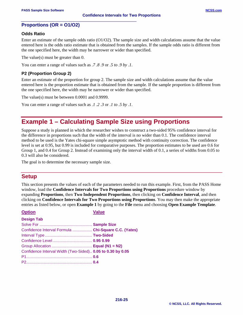
Example 1 – Calculating Sample Size using Proportions Suppose a study is planned in which the researcher wishes to construct a two-sided 95% confidence interval for the difference in proportions such that the width of the interval is no wider than 0.1. The confidence interval method to be used is the Yates chi-square simple asymptotic method with continuity correction. The confidence level is set at 0.95, but 0.99 is included for comparative purposes. The proportion estimates to be used are 0.6 for Group 1, and 0.4 for Group 2. Instead of examining only the interval width of 0.1, a series of widths from 0.05 to 0.3 will also be considered. The goal is to determine the necessary sample size.

Setup This section presents the values of each of the parameters needed to run this example. First, from the PASS Home window, load the Confidence Intervals for Two Proportions using Proportions procedure window by expanding Proportions, then Two Independent Proportions, then clicking on Confidence Interval, and then clicking on Confidence Intervals for Two Proportions using Proportions. You may then make the appropriate entries as listed below, or open Example 1 by going to the File menu and choosing Open Example Template.

Option Value Design Tab Solve For ................................................ Sample Size Confidence Interval Formula .................. Chi-Square C.C. (Yates) Interval Type ........................................... Two-Sided Confidence Level .................................... 0.95 0.99 Group Allocation ..................................... Equal (N1 = N2) Confidence Interval Width (Two-Sided) .. 0.05 to 0.30 by 0.05 P1............................................................ 0.6 P2............................................................ 0.4




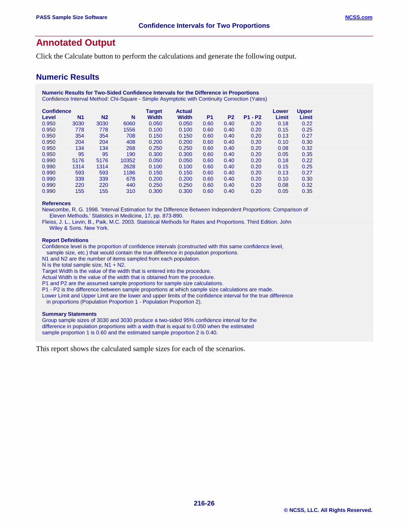
Annotated Output Click the Calculate button to perform the calculations and generate the following output.

Numeric Results

Numeric Results for Two-Sided Confidence Intervals for the Difference in Proportions Confidence Interval Method: Chi-Square - Simple Asymptotic with Continuity Correction (Yates) Confidence Target Actual Lower Upper Level N1 N2 N Width Width P1 P2 P1 - P2 Limit Limit 0.950 3030 3030 6060 0.050 0.050 0.60 0.40 0.20 0.18 0.22 0.950 778 778 1556 0.100 0.100 0.60 0.40 0.20 0.15 0.25 0.950 354 354 708 0.150 0.150 0.60 0.40 0.20 0.13 0.27 0.950 204 204 408 0.200 0.200 0.60 0.40 0.20 0.10 0.30 0.950 134 134 268 0.250 0.250 0.60 0.40 0.20 0.08 0.32 0.950 95 95 190 0.300 0.300 0.60 0.40 0.20 0.05 0.35 0.990 5176 5176 10352 0.050 0.050 0.60 0.40 0.20 0.18 0.22 0.990 1314 1314 2628 0.100 0.100 0.60 0.40 0.20 0.15 0.25 0.990 593 593 1186 0.150 0.150 0.60 0.40 0.20 0.13 0.27 0.990 339 339 678 0.200 0.200 0.60 0.40 0.20 0.10 0.30 0.990 220 220 440 0.250 0.250 0.60 0.40 0.20 0.08 0.32 0.990 155 155 310 0.300 0.300 0.60 0.40 0.20 0.05 0.35 References Newcombe, R. G. 1998. 'Interval Estimation for the Difference Between Independent Proportions: Comparison of Eleven Methods.' Statistics in Medicine, 17, pp. 873-890. Fleiss, J. L., Levin, B., Paik, M.C. 2003. Statistical Methods for Rates and Proportions. Third Edition. John Wiley & Sons. New York. Report Definitions Confidence level is the proportion of confidence intervals (constructed with this same confidence level, sample size, etc.) that would contain the true difference in population proportions. N1 and N2 are the number of items sampled from each population. N is the total sample size, N1 + N2. Target Width is the value of the width that is entered into the procedure. Actual Width is the value of the width that is obtained from the procedure. P1 and P2 are the assumed sample proportions for sample size calculations. P1 - P2 is the difference between sample proportions at which sample size calculations are made. Lower Limit and Upper Limit are the lower and upper limits of the confidence interval for the true difference in proportions (Population Proportion 1 - Population Proportion 2). Summary Statements Group sample sizes of 3030 and 3030 produce a two-sided 95% confidence interval for the difference in population proportions with a width that is equal to 0.050 when the estimated sample proportion 1 is 0.60 and the estimated sample proportion 2 is 0.40.

This report shows the calculated sample sizes for each of the scenarios.




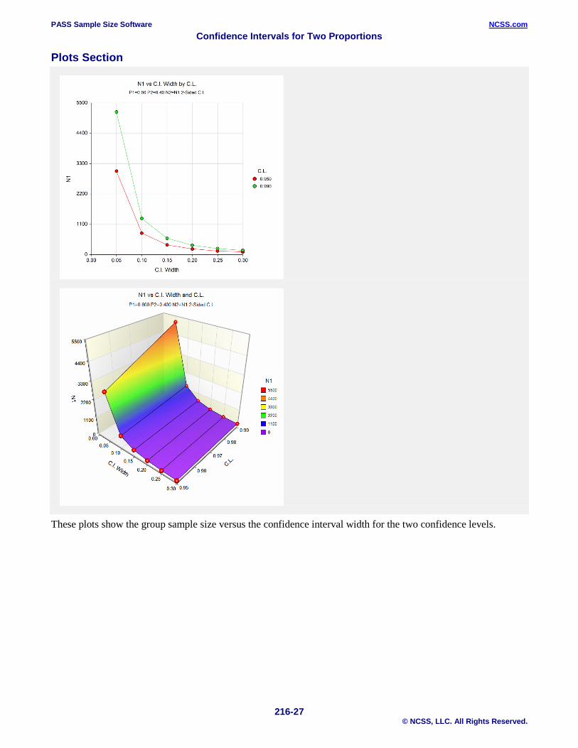
Plots Section

These plots show the group sample size versus the confidence interval width for the two confidence levels.




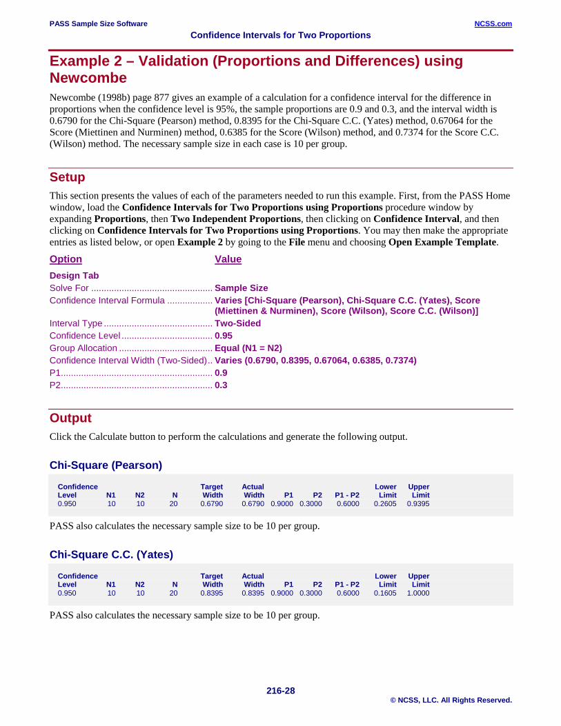
Example 2 – Validation (Proportions and Differences) using Newcombe Newcombe (1998b) page 877 gives an example of a calculation for a confidence interval for the difference in proportions when the confidence level is 95%, the sample proportions are 0.9 and 0.3, and the interval width is 0.6790 for the Chi-Square (Pearson) method, 0.8395 for the Chi-Square C.C. (Yates) method, 0.67064 for the Score (Miettinen and Nurminen) method, 0.6385 for the Score (Wilson) method, and 0.7374 for the Score C.C. (Wilson) method. The necessary sample size in each case is 10 per group.


Option Value Design Tab Solve For ................................................ Sample Size Confidence Interval Formula .................. Varies [Chi-Square (Pearson), Chi-Square C.C. (Yates), Score

(Miettinen & Nurminen), Score (Wilson), Score C.C. (Wilson)] Interval Type ........................................... Two-Sided Confidence Level .................................... 0.95 Group Allocation ..................................... Equal (N1 = N2) Confidence Interval Width (Two-Sided) .. Varies (0.6790, 0.8395, 0.67064, 0.6385, 0.7374) P1............................................................ 0.9 P2............................................................ 0.3

Output Click the Calculate button to perform the calculations and generate the following output.

Chi-Square (Pearson)

Confidence Target Actual Lower Upper Level N1 N2 N Width Width P1 P2 P1 - P2 Limit Limit 0.950 10 10 20 0.6790 0.6790 0.9000 0.3000 0.6000 0.2605 0.9395

PASS also calculates the necessary sample size to be 10 per group.

Chi-Square C.C. (Yates)






Score (Miettinen & Nurminen)



Score (Wilson)



Score C.C. (Wilson)






Example 3 – Validation (Proportions and Differences) using Gart and Nam Gart and Nam (1990) page 640 give an example of a calculation for a confidence interval for the difference in proportions when the confidence level is 95%, the sample proportions are 0.28 and 0.08, and the interval width is 0.4281 for the Score (Gart and Nam) method. The necessary sample size in each case is 25 per group.


Option Value Design Tab Solve For ................................................ Sample Size Confidence Interval Formula .................. Score w/Skewness (Gart & Nam) Interval Type ........................................... Two-Sided Confidence Level .................................... 0.95 Group Allocation ..................................... Equal (N1 = N2) Confidence Interval Width (Two-Sided) .. 0.4281 P1............................................................ 0.28 P2............................................................ 0.08


Numeric Results

Confidence Target Actual Lower Upper Level N1 N2 N Width Width P1 P2 P1 - P2 Limit Limit 0.950 25 25 50 0.4281 0.4281 0.2800 0.0800 0.2000 -0.0143 0.4137





Example 4 – Calculating Sample Size using Differences Suppose a study is planned in which the researcher wishes to construct a two-sided 95% confidence interval for the difference in proportions such that the width of the interval is no wider than 0.1. The confidence interval method to be used is the Yates chi-square simple asymptotic method with continuity correction. The confidence level is set at 0.95, but 0.99 is included for comparative purposes. The difference estimate to be used is 0.05, and the estimate for proportion 2 is 0.3. Instead of examining only the interval width of 0.1, a series of widths from 0.05 to 0.3 will also be considered. The goal is to determine the necessary sample size.

Setup This section presents the values of each of the parameters needed to run this example. First, from the PASS Home window, load the Confidence Intervals for Two Proportions using Differences procedure window by expanding Proportions, then Two Independent Proportions, then clicking on Confidence Interval, and then clicking on Confidence Intervals for Two Proportions using Differences. You may then make the appropriate entries as listed below, or open Example 4 by going to the File menu and choosing Open Example Template.

Option Value Design Tab Solve For ................................................ Sample Size Confidence Interval Formula .................. Chi-Square C.C. (Yates) Interval Type ........................................... Two-Sided Confidence Level .................................... 0.95 0.99 Group Allocation ..................................... Equal (N1 = N2) Confidence Interval Width (Two-Sided) .. 0.05 to 0.30 by 0.05 Difference in Sample Proportions ........... 0.05 P2............................................................ 0.3


Numeric Results

Numeric Results for Two-Sided Confidence Intervals for the Difference in Proportions Confidence Interval Method: Chi-Square - Simple Asymptotic with Continuity Correction (Yates) Confidence Target Actual Lower Upper Level N1 N2 N Width Width P1 P2 P1 - P2 Limit Limit 0.950 2769 2769 5538 0.050 0.050 0.35 0.30 0.05 0.03 0.07 0.950 712 712 1424 0.100 0.100 0.35 0.30 0.05 0.00 0.10 0.950 325 325 650 0.150 0.150 0.35 0.30 0.05 -0.02 0.12 0.950 188 188 376 0.200 0.200 0.35 0.30 0.05 -0.05 0.15 0.950 124 124 248 0.250 0.249 0.35 0.30 0.05 -0.07 0.17 0.950 88 88 176 0.300 0.299 0.35 0.30 0.05 -0.10 0.20 0.990 4725 4725 9450 0.050 0.050 0.35 0.30 0.05 0.03 0.07 0.990 1201 1201 2402 0.100 0.100 0.35 0.30 0.05 0.00 0.10 0.990 543 543 1086 0.150 0.150 0.35 0.30 0.05 -0.02 0.12 0.990 310 310 620 0.200 0.200 0.35 0.30 0.05 -0.05 0.15 0.990 202 202 404 0.250 0.250 0.35 0.30 0.05 -0.07 0.17 0.990 143 143 286 0.300 0.299 0.35 0.30 0.05 -0.10 0.20




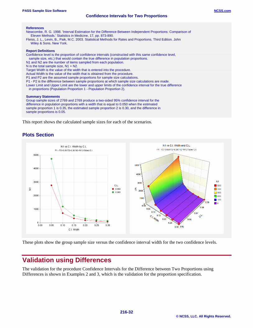
References Newcombe, R. G. 1998. 'Interval Estimation for the Difference Between Independent Proportions: Comparison of Eleven Methods.' Statistics in Medicine, 17, pp. 873-890. Fleiss, J. L., Levin, B., Paik, M.C. 2003. Statistical Methods for Rates and Proportions. Third Edition. John Wiley & Sons. New York. Report Definitions Confidence level is the proportion of confidence intervals (constructed with this same confidence level, sample size, etc.) that would contain the true difference in population proportions. N1 and N2 are the number of items sampled from each population. N is the total sample size, N1 + N2. Target Width is the value of the width that is entered into the procedure. Actual Width is the value of the width that is obtained from the procedure. P1 and P2 are the assumed sample proportions for sample size calculations. P1 - P2 is the difference between sample proportions at which sample size calculations are made. Lower Limit and Upper Limit are the lower and upper limits of the confidence interval for the true difference in proportions (Population Proportion 1 - Population Proportion 2). Summary Statements Group sample sizes of 2769 and 2769 produce a two-sided 95% confidence interval for the difference in population proportions with a width that is equal to 0.050 when the estimated sample proportion 1 is 0.35, the estimated sample proportion 2 is 0.30, and the difference in sample proportions is 0.05.


Plots Section


Validation using Differences The validation for the procedure Confidence Intervals for the Difference between Two Proportions using Differences is shown in Examples 2 and 3, which is the validation for the proportion specification.




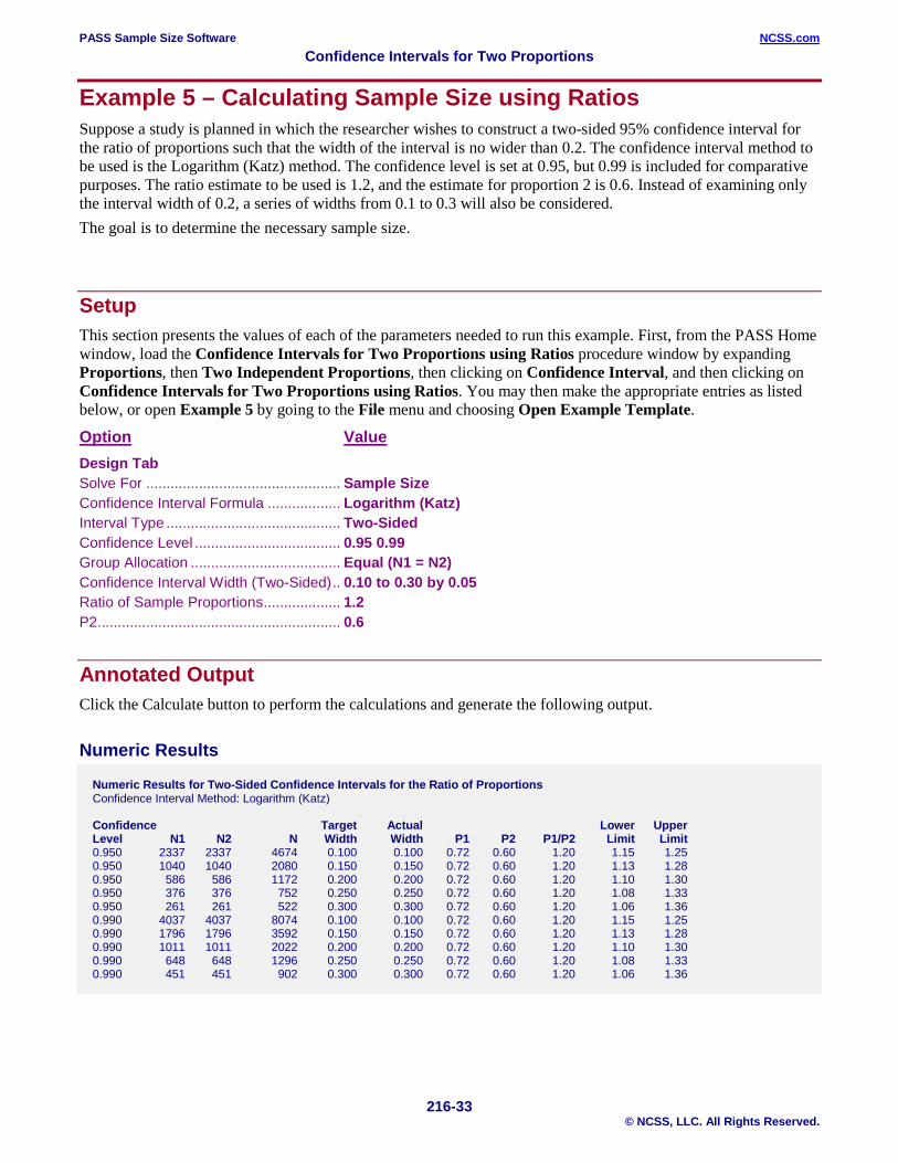
Example 5 – Calculating Sample Size using Ratios Suppose a study is planned in which the researcher wishes to construct a two-sided 95% confidence interval for the ratio of proportions such that the width of the interval is no wider than 0.2. The confidence interval method to be used is the Logarithm (Katz) method. The confidence level is set at 0.95, but 0.99 is included for comparative purposes. The ratio estimate to be used is 1.2, and the estimate for proportion 2 is 0.6. Instead of examining only the interval width of 0.2, a series of widths from 0.1 to 0.3 will also be considered. The goal is to determine the necessary sample size.

Setup This section presents the values of each of the parameters needed to run this example. First, from the PASS Home window, load the Confidence Intervals for Two Proportions using Ratios procedure window by expanding Proportions, then Two Independent Proportions, then clicking on Confidence Interval, and then clicking on Confidence Intervals for Two Proportions using Ratios. You may then make the appropriate entries as listed below, or open Example 5 by going to the File menu and choosing Open Example Template.

Option Value Design Tab Solve For ................................................ Sample Size Confidence Interval Formula .................. Logarithm (Katz) Interval Type ........................................... Two-Sided Confidence Level .................................... 0.95 0.99 Group Allocation ..................................... Equal (N1 = N2) Confidence Interval Width (Two-Sided) .. 0.10 to 0.30 by 0.05 Ratio of Sample Proportions ................... 1.2 P2............................................................ 0.6


Numeric Results

Numeric Results for Two-Sided Confidence Intervals for the Ratio of Proportions Confidence Interval Method: Logarithm (Katz) Confidence Target Actual Lower Upper Level N1 N2 N Width Width P1 P2 P1/P2 Limit Limit 0.950 2337 2337 4674 0.100 0.100 0.72 0.60 1.20 1.15 1.25 0.950 1040 1040 2080 0.150 0.150 0.72 0.60 1.20 1.13 1.28 0.950 586 586 1172 0.200 0.200 0.72 0.60 1.20 1.10 1.30 0.950 376 376 752 0.250 0.250 0.72 0.60 1.20 1.08 1.33 0.950 261 261 522 0.300 0.300 0.72 0.60 1.20 1.06 1.36 0.990 4037 4037 8074 0.100 0.100 0.72 0.60 1.20 1.15 1.25 0.990 1796 1796 3592 0.150 0.150 0.72 0.60 1.20 1.13 1.28 0.990 1011 1011 2022 0.200 0.200 0.72 0.60 1.20 1.10 1.30 0.990 648 648 1296 0.250 0.250 0.72 0.60 1.20 1.08 1.33 0.990 451 451 902 0.300 0.300 0.72 0.60 1.20 1.06 1.36




References Gart, John J. and Nam, Jun-mo. 1988. 'Approximate Interval Estimation of the Ratio of Binomial Parameters: A Review and Corrections for Skewness.' Biometrics, Volume 44, 323-338. Koopman, P. A. R. 1984. 'Confidence Intervals for the Ratio of Two Binomial Proportions.' Biometrics, Volume 40, Issue 2, 513-517. Katz, D., Baptista, J., Azen, S. P., and Pike, M. C. 1978. 'Obtaining Confidence Intervals for the Risk Ratio in Cohort Studies.' Biometrics, Volume 34, 469-474. Report Definitions Confidence level is the proportion of confidence intervals (constructed with this same confidence level, sample size, etc.) that would contain the true ratio of population proportions. N1 and N2 are the number of items sampled from each population. N is the total sample size, N1 + N2. Target Width is the value of the width that is entered into the procedure. Actual Width is the value of the width that is obtained from the procedure. P1 and P2 are the assumed sample proportions for sample size calculations. P1/P2 is the ratio of sample proportions at which sample size calculations are made. Lower Limit and Upper Limit are the lower and upper limits of the confidence interval for the true ratio of proportions (Population Proportion 1 / Population Proportion 2). Summary Statements Group sample sizes of 2337 and 2337 produce a two-sided 95% confidence interval for the ratio of population proportions with a width that is equal to 0.100 when the estimated sample proportion 1 is 0.72, the estimated sample proportion 2 is 0.60, and the ratio of the sample proportions is 1.20.


Plots Section





Example 6 – Validation (Ratios) using Gart and Nam Gart and Nam (1988) page 331 give an example (Example 2) of a calculation for a confidence interval for the ratio of proportions when the confidence level is 95%, the sample proportion ratio is 2 and the sample proportion 2 is 0.3, the sample size for group 2 is 20, and the interval width is 3.437 for the Logarithm + 1/2 (Walter) method, 3.751 for the Score (Farrington and Manning) method, and 4.133 for the Score w/Skewness (Gart and Nam) method. The necessary sample size for group 1 in each case is 10.


Option Value Design Tab Solve For ................................................ Sample Size Confidence Interval Formula .................. Varies [Logarithm + 1/2 (Walter), Score (Farrington and Manning),

Score w/Skewness (Gart and Nam)] Interval Type ........................................... Two-Sided Confidence Level .................................... 0.95 Group Allocation ..................................... Enter N2, solve for N1 N2 ........................................................... 20 Confidence Interval Width (Two-Sided) .. Varies (3.437, 3.751, 4.133) Ratio of Sample Proportions ................... 2 P2............................................................ 0.3


Logarithm + 1/2 (Walter)

Confidence Target Actual Lower Upper Level N1 N2 N Width Width P1 P2 P1/P2 Limit Limit 0.950 10 20 30 3.437 3.431 0.60 0.30 2.00 0.88 4.31

PASS also calculates the necessary sample size for Group 1 to be 10.

Score (Farrington and Manning)






Score w/Skewness (Gart and Nam)



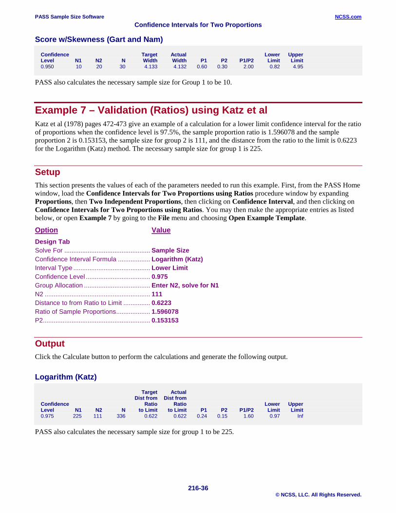
Example 7 – Validation (Ratios) using Katz et al Katz et al (1978) pages 472-473 give an example of a calculation for a lower limit confidence interval for the ratio of proportions when the confidence level is 97.5%, the sample proportion ratio is 1.596078 and the sample proportion 2 is 0.153153, the sample size for group 2 is 111, and the distance from the ratio to the limit is 0.6223 for the Logarithm (Katz) method. The necessary sample size for group 1 is 225.


Option Value Design Tab Solve For ................................................ Sample Size Confidence Interval Formula .................. Logarithm (Katz) Interval Type ........................................... Lower Limit Confidence Level .................................... 0.975 Group Allocation ..................................... Enter N2, solve for N1 N2 ........................................................... 111 Distance to from Ratio to Limit ............... 0.6223 Ratio of Sample Proportions ................... 1.596078 P2............................................................ 0.153153


Logarithm (Katz)

Target Actual Dist from Dist from Confidence Ratio Ratio Lower Upper Level N1 N2 N to Limit to Limit P1 P2 P1/P2 Limit Limit 0.975 225 111 336 0.622 0.622 0.24 0.15 1.60 0.97 Inf

PASS also calculates the necessary sample size for group 1 to be 225.




Example 8 – Calculating Sample Size using Odds Ratios Suppose a study is planned in which the researcher wishes to construct a two-sided 95% confidence interval for the odds ratio such that the width of the interval is no wider than 0.5. The confidence interval method to be used is the Logarithm method. The confidence level is set at 0.95, but 0.99 is included for comparative purposes. The odds ratio estimate to be used is 1.5, and the estimate for proportion 2 is 0.4. Instead of examining only the interval width of 0.5, a series of widths from 0.1 to 1.0 will also be considered. The goal is to determine the necessary sample size.

Setup This section presents the values of each of the parameters needed to run this example. First, from the PASS Home window, load the Confidence Intervals for Two Proportions using Odds Ratios procedure window by expanding Proportions, then Two Independent Proportions, then clicking on Confidence Interval, and then clicking on Confidence Intervals for Two Proportions using Odds Ratios. You may then make the appropriate entries as listed below, or open Example 8 by going to the File menu and choosing Open Example Template.

Option Value Design Tab Solve For ................................................ Sample Size Confidence Interval Formula .................. Logarithm Interval Type ........................................... Two-Sided Confidence Level .................................... 0.95 0.99 Group Allocation ..................................... Equal (N1 = N2) Confidence Interval Width (Two-Sided) .. 0.1 to 1.0 by 0.1 Odds Ratio .............................................. 1.5 P2............................................................ 0.4


Numeric Results

Numeric Results for Two-Sided Confidence Intervals for the Odds Ratio Confidence Interval Method: Logarithm Odds Confidence Target Actual Ratio Lower Upper Level N1 N2 N Width Width P1 P2 O1/O2 Limit Limit 0.950 28244 28244 56488 0.100 0.100 0.50 0.40 1.50 1.45 1.55 0.950 7068 7068 14136 0.200 0.200 0.50 0.40 1.50 1.40 1.60 0.950 3146 3146 6292 0.300 0.300 0.50 0.40 1.50 1.36 1.66 0.950 1774 1774 3548 0.400 0.400 0.50 0.40 1.50 1.31 1.71 0.950 1138 1138 2276 0.500 0.500 0.50 0.40 1.50 1.27 1.77 0.950 793 793 1586 0.600 0.600 0.50 0.40 1.50 1.23 1.83 0.950 585 585 1170 0.700 0.700 0.50 0.40 1.50 1.19 1.89 0.950 450 450 900 0.800 0.800 0.50 0.40 1.50 1.15 1.95 0.950 358 358 716 0.900 0.899 0.50 0.40 1.50 1.11 2.01 0.950 291 291 582 1.000 1.000 0.50 0.40 1.50 1.08 2.08 0.990 48783 48783 97566 0.100 0.100 0.50 0.40 1.50 1.45 1.55 0.990 12208 12208 24416 0.200 0.200 0.50 0.40 1.50 1.40 1.60 0.990 5435 5435 10870 0.300 0.300 0.50 0.40 1.50 1.36 1.66 0.990 3065 3065 6130 0.400 0.400 0.50 0.40 1.50 1.31 1.71 0.990 1967 1967 3934 0.500 0.500 0.50 0.40 1.50 1.27 1.77 0.990 1371 1371 2742 0.600 0.600 0.50 0.40 1.50 1.23 1.83




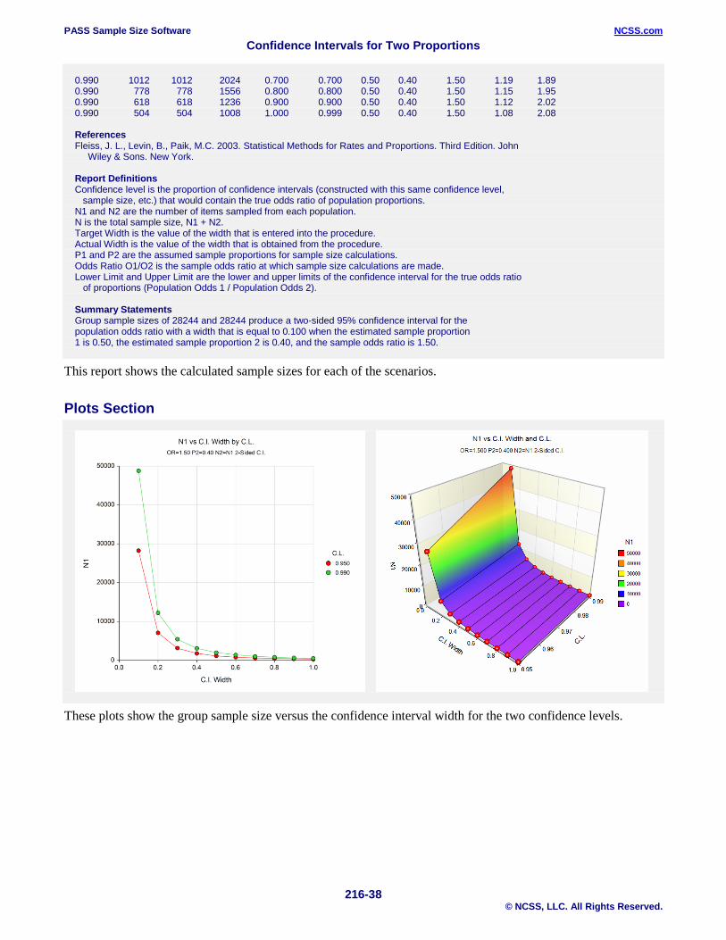
0.990 1012 1012 2024 0.700 0.700 0.50 0.40 1.50 1.19 1.89 0.990 778 778 1556 0.800 0.800 0.50 0.40 1.50 1.15 1.95 0.990 618 618 1236 0.900 0.900 0.50 0.40 1.50 1.12 2.02 0.990 504 504 1008 1.000 0.999 0.50 0.40 1.50 1.08 2.08 References Fleiss, J. L., Levin, B., Paik, M.C. 2003. Statistical Methods for Rates and Proportions. Third Edition. John Wiley & Sons. New York. Report Definitions Confidence level is the proportion of confidence intervals (constructed with this same confidence level, sample size, etc.) that would contain the true odds ratio of population proportions. N1 and N2 are the number of items sampled from each population. N is the total sample size, N1 + N2. Target Width is the value of the width that is entered into the procedure. Actual Width is the value of the width that is obtained from the procedure. P1 and P2 are the assumed sample proportions for sample size calculations. Odds Ratio O1/O2 is the sample odds ratio at which sample size calculations are made. Lower Limit and Upper Limit are the lower and upper limits of the confidence interval for the true odds ratio of proportions (Population Odds 1 / Population Odds 2). Summary Statements Group sample sizes of 28244 and 28244 produce a two-sided 95% confidence interval for the population odds ratio with a width that is equal to 0.100 when the estimated sample proportion 1 is 0.50, the estimated sample proportion 2 is 0.40, and the sample odds ratio is 1.50.


Plots Section





Example 9 – Validation (Odds Ratios) using Fleiss et al Fleiss et al (2003) pages 117, 119 give an example of a calculation for a confidence interval for the odds ratio when the confidence level is 95%, the sample odds ratio is 2.25 and the sample proportion 2 is 0.1, the sample size for group 2 is 150, and the interval width is 4.387 for the Logarithm method, and 4.980 for the Fleiss method. The necessary sample size for group 1 in each case is 50.

Setup This section presents the values of each of the parameters needed to run this example. First, from the PASS Home window, load the Confidence Intervals for Two Proportions using Odds Ratios procedure window by expanding Proportions, then Two Independent Proportions, then clicking on Confidence Interval, and then clicking on Confidence Intervals for Two Proportions using Odds Ratios. You may then make the appropriate entries as listed below, or open Example 9 by going to the File menu and choosing Open Example Template.

Option Value Design Tab Solve For ................................................ Sample Size Confidence Interval Formula .................. Varies [Logarithm, Fleiss] Interval Type ........................................... Two-Sided Confidence Level .................................... 0.95 Group Allocation ..................................... Enter N2, solve for N1 N2 ........................................................... 150 Confidence Interval Width (Two-Sided) .. Varies (4.387, 4.980) Odds Ratio .............................................. 2.25 P2............................................................ 0.1


Logarithm

Odds Confidence Target Actual Ratio Lower Upper Level N1 N2 N Width Width P1 P2 O1/O2 Limit Limit 0.950 50 150 200 4.387 4.387 0.20 0.10 2.25 0.96 5.35


Fleiss

Odds Confidence Target Actual Ratio Lower Upper Level N1 N2 N Width Width P1 P2 O1/O2 Limit Limit 0.950 50 150 200 4.980 4.980 0.20 0.10 2.25 0.86 5.84



confidence intervals for two proportions - ncss.com€¦ · a background of the comparison of two...

Documents