confidence intervals for population forecasts: a case ... reports... · confidence intervals for...

Confidence Intervals for Population Forecasts: A Case Study of Time Series Models for States

Stanley K. Smith, University of Florida

Jeff Tayman, San Diego Association of Governments

Paper presented at the annual meeting of the

Population Association of America, Boston, April 1-3, 2004

2

ABSTRACT

A number of studies have dealt with the use of time series models to develop confidence intervals for population forecasts. Most have focused solely on national-level models and only a few have considered the accuracy of the resulting forecasts. In this study, we take this research in a new direction by constructing time series models for several states in the United States and evaluating the resulting population forecasts. Using annual population estimates from 1900 to 2000, we develop a variety of forecasts and investigate the impact of differences in model specification, state, launch year, length of base period, and length of forecast horizon on the accuracy of point forecasts and the width of confidence intervals. We also evaluate the extent to which predicted confidence intervals encompass future population counts. We conclude with several observations regarding the potential usefulness of time series models for forecasting state populations.

3

INTRODUCTION

A number of studies have considered the use of time series models for developing

confidence intervals to accompany population forecasts (e.g., Alho and Spencer 1997; De Beer

1993; Keilman, Pham, and Hetland 2002; Lee 1974, 1992, 1999; Lee and Tuljapurkar 1994;

McNown and Rogers 1989; Pflaumer 1992). Some have developed models of total population

growth, whereas others have developed models of the individual components of growth—

especially mortality and fertility—by age and sex. Studies of both types have typically focused

on the sources of uncertainty in population forecasts, how to develop models that provide

specific measures of that uncertainty, and how the resulting point forecasts and confidence

intervals compare with those produced by other models. Most of these studies have dealt solely

with national-level models and only a few have considered the accuracy of the resulting

forecasts.

To our knowledge, only one study has developed and evaluated time series models for

states. Voss, Palit, Kale, and Krebs (1981) developed and tested several ARIMA models for

states and chose a single model for their detailed analyses. They used this model to construct

population forecasts for the 48 coterminous states in the United States, using a number of launch

years and forecast horizons. This study evaluated accuracy by comparing the resulting forecasts

with census counts and census-based population estimates. It also compared the accuracy of the

ARIMA forecasts with the accuracy of several other forecasting models and found them to be

roughly the same. The authors briefly discussed the use of ARIMA models for constructing

confidence intervals, but did not pursue that line of research.

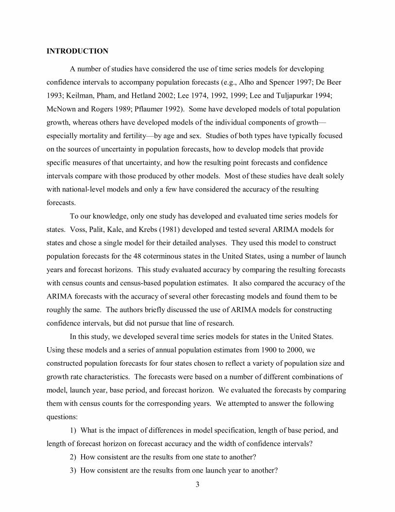
In this study, we developed several time series models for states in the United States.

Using these models and a series of annual population estimates from 1900 to 2000, we

constructed population forecasts for four states chosen to reflect a variety of population size and

growth rate characteristics. The forecasts were based on a number of different combinations of

model, launch year, base period, and forecast horizon. We evaluated the forecasts by comparing

them with census counts for the corresponding years. We attempted to answer the following

questions:

1) What is the impact of differences in model specification, length of base period, and

length of forecast horizon on forecast accuracy and the width of confidence intervals?

2) How consistent are the results from one state to another?

3) How consistent are the results from one launch year to another?

4

4) What proportion of future populations fall with the predicted confidence intervals?

Time series forecasting models are subject to errors in the base data, errors in specifying

the model, errors in estimating the model’s parameters, and structural changes that invalidate the

model’s statistical relationships (Lee 1992). Furthermore, many different models can be

specified, each providing a different set of confidence intervals (e.g., Lee 1974; Cohen 1986;

Sanderson 1995; Keilman, Pham, and Hetland 2002). To date, few studies have investigated the

accuracy of time series population forecasting models or have considered their use for

subnational areas. We believe the present study helps to fill that void.

ARIMA MODELING

A number of different time series models can be used for forecasting purposes. In this

study, we used univariate ARIMA models based on past population values and the dynamic and

stochastic properties of error terms. Like other extrapolation methods, these models do not

require knowledge of the underlying structural relationships; rather, they are based on the

assumption that past population values provide sufficient information for forecasting future

values. The two main advantages of univariate ARIMA models are: 1) they require historical

data only on the total population of the area being forecasted; and 2) their underlying

mathematical and statistical properties provide a basis for developing probabilistic intervals to

accompany point forecasts (Nelson 1973). The methods used for developing ARIMA models,

however, are more complex and subjective in their application than are most extrapolation

methods.

We developed several ARIMA models using the approach and techniques popularized by

Box and Jenkins (1976). The most general ARIMA model is usually expressed as ARIMA

(p,d,q), where p is the order of the autoregressive term, d is the degree of differencing, and q is

the order of the moving average term.1 Identification is the first (and most ambiguous) step in

building ARIMA models (McCleary and Hay 1980). Model identification refers to the process

for determining the values of p, d, and q, which typically range from 0 to 2. The d value must be

determined first because a stationary time series (i.e., one in which the mean and variance are

constant over time) is required to properly identify the values of p and q. When a time series is

not stationary, it can generally be converted into a stationary series by taking first or second

differences (Saboia 1974). Logarithmic, square root, and other transformations can also be used.

The main tools for model identification are the patterns and standard errors of the

autocorrelation function (ACF) and partial autocorrelation function (PACF). A first-order

5

autoregressive model ARIMA (1,0,0), for example, is characterized by an ACF that declines

exponentially and quickly and a PACF that has a statistically significant spike only at the first

lag. Other statistics and criteria such as the Dickey Fuller Test and the Akaike Information

Criterion can also be used to help identify an ARIMA model (Meyler, Kenny, and Quinn 1998).

After the p, d, and q values have been determined, maximum likelihood procedures are used to

estimate the model’s parameters. The final step is model diagnosis. A statistically adequate

ARIMA model will have random residuals, no significant values in the ACF and PACF, and the

smallest possible values for p, d, and q. Because a good statistical fit does not guarantee an

accurate or even a reasonable forecast, it may also be useful to perform an N-step ahead, out-of-

sample evaluation of the accuracy and bias of the model (Granger 1989; Meyler, Kenny, and

Quinn 1998).

We analyzed four ARIMA models that have been used to forecast population growth or

the components of population change. As noted below, we fit each model for each state using 15

different combinations of base period and launch year. Our objective was not to find the “best”

model for each combination, but rather to study the behavior of commonly used specifications

that reflect different assumptions about future growth trajectories. In fact, an examination of the

autocorrelation and partial autocorrelation plots and associated statistics revealed that no single

ARIMA specification provided a reasonable fit across all 60 combinations of base period, launch

year, and state. Moreover, given that some of our base periods contained as few as 10

observations, the identification process did not always clearly suggest a single ARIMA

specification for each of the 60 combinations.2

Models 1 and 3 contain only first-order terms and suggest that future growth will follow a

linear pattern. Model 1 contains a first-order autoregressive term with first differences and no

moving average term; it is identified as ARIMA (1,1,0). This model has been widely used for

population forecasts (e.g., Cohen 1986; Saboia 1974; Smith and Sincich 1992) and some analysts

have found it to outperform more complex time series formulations (e.g., Voss and Kale 1985;

Voss, et al. 1981). Model 3 contains a first-order moving average term with first differences and

no autoregressive term; it is identified as ARIMA (0,1,1). Models of this type have been used by

Alho (1990) and De Beer (1993).3

Models 2 and 4 are nonlinear, containing at least one second-order term. In these models,

population follows a different (most likely faster) growth trajectory than in Models 1 and 3.

Model 2 contains a second-order autoregressive term with second differences and no moving

6

average term; it is identified as ARIMA (2,2,0). Pflaumer (1992) has shown that Model 2 is

equivalent to a parabolic, quadratic trend model. Model 4 contains a first-order moving average

term with second differences and no autoregressive term; it is identified as ARIMA (0,2,1).

Models of this type have been used by Cohen (1986) and Saboia (1974). Some analysts have

suggested that second differences may be best for modeling human populations and have

provided evidence that models containing higher order differences may outperform models using

only first differences (e.g., McKnown and Rogers 1989; Saboia 1974).

DATA

We wanted to test the four ARIMA models in states exhibiting a variety of size and

growth characteristics. Using a set of state population estimates produced by the U.S. Census

Bureau for each year between 1900 and 2000 (U.S. Census Bureau 1956, 1965, 1971, 1984,

1993, and 2002), we chose four states with widely varying size and growth characteristics:

Florida, Maine, Ohio, and Wyoming. Using these states allows us to test the models under a

variety of demographic scenarios.

Wyoming is the smallest state in the nation, with a population of barely half a million in

2003 (U.S. Census Bureau 2003). As shown in Table 1, its growth rates have fluctuated

considerably from one decade to the next, including one decade with negative growth. Maine is

also a small state (1.3 million in 2003), but it exhibited moderate and relatively stable growth

rates throughout the twentieth century. Florida is the 4th largest state in the nation, with just over

17 million residents in 2003. Florida has grown rapidly but unevenly since 1900, with growth

rates ranging between 27% and 78% per decade. Ohio is the 7th largest state, with a population

of 11.4 million in 2003. Ohio has grown much less rapidly than Florida, but its growth rates

have also fluctuated considerably from one decade to the next.

(Table 1 about here)

These four states followed markedly different population growth patterns during the 20th

century. Florida’s population grew by 13.2 million between 1950 and 2000, compared to only

2.3 million between 1900 and 1950. Maine also added more residents during the second half of

the century than the first half: 360,000 compared to 222,000. Growth in Wyoming was about the

same in both time periods, as the state added 197,000 residents between 1900 and 1950 and

204,000 between 1950 and 2000. Ohio was the only state in our sample that added fewer

residents in the second half of the century than the first half, growing by 3.8 million between

1900 and 1950 and by 3.4 million between 1950 and 2000.

7

ANALYSES

We applied each of the four models to each state using three launch years (1950, 1960,

and 1970), base periods of five lengths (10, 20, 30, 40, and 50 years), and forecast horizons of

three lengths (10, 20, and 30 years). This gave a total of 180 point forecasts and associated

confidence intervals for each state. We compared each point forecast to the population count for

the relevant target year. We refer to the resulting percentage differences as forecast errors,

although they may have been caused partly by errors in the population counts themselves.

Following Lee and Tuljapurkar (1994), we express the size of the confidence interval as a half-

width by dividing one-half of the difference between the upper and lower ends of the interval by

the point forecast. We calculated half-widths for both 95% and 68% confidence intervals; in this

paper, we report only the latter.

Trying to analyze errors and half-widths for 720 forecasts is, of course, a difficult task.

To simplify the analysis, we started by lumping together the forecasts from each of the four

states and three launch years, and calculating the average error and average half-width of these

12 forecasts for each combination of model, length of base period, and length of forecast

horizon. Then, we evaluated the results separately for each state and each launch year. Errors

were measured in two ways. The mean absolute percent error (MAPE) is the average when the

direction of error is ignored; it is a measure of precision. The mean algebraic percent error

(MALPE) is the average when the direction of error is accounted for; it is a measure of bias.

Results Averaged Over All States and Launch Years

The results averaged over states and launch years are shown in Tables 2-4. Several

patterns stand out. First, the results for Models 1 and 3 were very similar. For every

combination of base period and forecast horizon, the MAPEs, MALPEs, and half-widths were

almost the same for Model 3 as for Model 1. Both of these are linear models and it appears that

the inclusion or omission of the first-order autoregressive term and the moving average term had

little impact on the resulting forecasts.

(Tables 2-4 about here)

Second, MAPEs and MALPEs for Models 2 and 4 were similar to each other, but the

half-widths were not. For every combination of base period and forecast horizon, half-widths

were much larger for Model 2 than Model 4. Apparently, differences in the specification of the

8

two nonlinear models had little impact on precision and bias but had a substantial impact on the

measurement of uncertainty.

Third, MAPEs and half-widths were generally smaller for Models 1 and 3 than for

Models 2 and 4. This result was found for almost every combination of base period and forecast

horizon. For MAPEs, differences between the two types of models were very large for 10-year

base periods but became steadily smaller as the base period increased; at 50 years, differences

were very small. For half-widths, differences between the two types of models were large for all

base periods, especially for longer forecast horizons. Linear models thus produced more precise

forecasts and narrower confidence intervals than nonlinear models.

Fourth, the impact of the length of the base period on forecast precision varied by model.

For Models 1 and 3, MAPEs increased with increases in the base period, whereas for Models 2

and 4, MAPEs declined with increases in the base period. These results were found for all three

forecast horizons. In this sample, then, 10 years of base data were sufficient to obtain maximum

precision for the two linear models, but for the two nonlinear models precision increased

continuously as more base data were added (although the increases became steadily smaller as

the base period became longer).

Fifth, increasing the length of the base period reduced the size of the half-width for every

model and every length of forecast horizon, indicating that additional base data reduced the

uncertainty associated with population forecasts (or, at least, this measure of uncertainty). The

reductions were particularly great for Models 2 and 4, especially for longer forecast horizons.

Sixth, Models 1 and 3 had a negative bias whereas Models 2 and 4 had a positive bias.

This result was found for every combination of base period and forecast horizon. That is, linear

models tended to produce forecasts that were too low and nonlinear models tended to produce

forecasts that were too high. Furthermore, the absolute value of the MALPEs became larger as

the horizon increased—both when MALPEs were positive and when they were negative—

indicating that the magnitude of the bias increased with the length of the forecast horizon.

Seventh, the impact of the length of the base period on MALPEs varied by model. For

Models 1 and 3, increasing the base period exacerbated the downward bias of the forecasts. For

Models 2 and 4, increasing the base period reduced the upward bias. As we note later in the

paper, these results were not found for all states and launch years.

Finally, both MAPEs and half-widths increased steadily with the length of the forecast

horizon. This result was found for every model and every base period. This is not surprising, of

9

course: Longer horizons create greater uncertainty and larger errors because they provide more

opportunities for growth to deviate from predicted trends. Similar results have been reported in

many previous studies (e.g., Cohen 1986; Smith and Sincich 1992; Voss et al. 1981).

Results by State

Several patterns are apparent when forecasts from the four states and three launch years

are averaged together. Do the same patterns appear when the averages of the three launch years

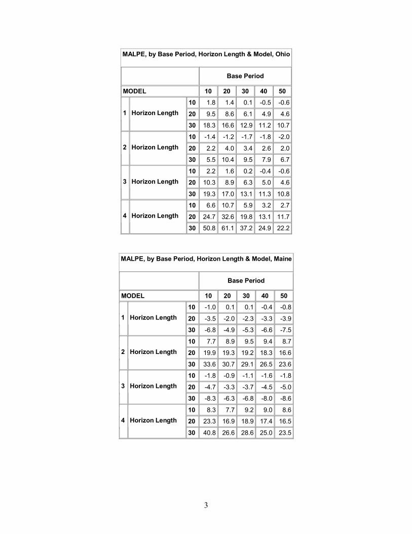
are calculated separately for each state? For the most part, yes (see Appendix A for details).

For every state and all combinations of forecast horizon and base period, MAPEs for

Model 1 were very similar to those for Model 3. In most instances, they were smaller than the

corresponding MAPEs for Models 2 and 4 (especially in Maine and Wyoming). MAPEs for

Models 2 and 4 occasionally were similar to each other, but often differed considerably;

sometimes the MAPE for Model 2 was larger, sometimes the MAPE for Model 4 was larger. In

most instances, MAPEs increased monotonically with the length of the horizon.

For Models 1 and 3, increasing the length of the base period had little impact on MAPEs

in Maine, Wyoming, and Ohio. In Florida, however, increasing the length of the base period

consistently raised MAPEs for both models. For Models 2 and 4, increasing the length of the

base period generally reduced MAPEs, especially for longer horizons. In many instances, the

reductions were fairly large when the base period was raised from 10 to 20 to 30 years, but fairly

small thereafter.

For every state, model, and forecast horizon, MALPEs for Models 1 and 3 were very

similar to each other. For Models 2 and 4, however, MALPEs often differed considerably from

each other. The direction of the bias varied by model and by state. In most instances, MALPEs

for Models 1 and 3 had negative signs for Maine, Wyoming, and Florida and positive signs for

Ohio. For Models 2 and 4, MALPEs generally had positive signs for Maine, Wyoming, and

Ohio and negative signs for Florida.

Bias generally increased with the length of the forecast horizon. If MALPEs were

positive for 10-year horizons, they generally became larger positive numbers as the horizon

increased. If they were negative for 10-year horizons, they generally became larger negative

numbers as the horizon increased. This occurred for almost all combinations of state, model, and

base period. The only exception was when MALPEs for 10-year horizons were close to zero; in

these instances, the impact of increases in length of horizon was inconsistent across states,

models, and base periods.

10

The impact of the length of the base period on MALPEs varied by state and model. For

Florida, increasing the base period increased the negative bias for Models 1, 2, and 3 (sometimes

substantially), but had no consistent effect for Model 4. For Wyoming, it substantially reduced

the upward bias for Models 2 and 4, but had little effect for Models 1 and 3. For Ohio, it

generally reduced the upward bias, but the effects were very small for some models and

horizons. For Maine, it sometimes exacerbated the upward or downward biases, but generally

had little impact. There does not appear to be any consistent relationship between bias and the

length of the base period.

For all states, horizons, and base periods, half-widths for Models 1 and 3 were similar to

each other, but the degree of similarity was not quite as high as it was for MAPEs. In most

instances, half-widths for Models 1 and 3 were considerably smaller than half-widths for Models

2 and 4. Model 2 generally had the largest half-width of all four models. For all states, models,

and base periods, half-widths increased with the length of the horizon; in many instances, the

increases were quite large.

For most combinations of state, model, and horizon, increasing the base period reduced

the half-width (often monotonically). The reductions were especially large for Models 2 and 4,

and were generally greater for longer horizons than for shorter horizons. The only exception was

Model 1 in Florida, where increasing the base period had very little effect on the half-width.

The impact of differences in base period, forecast horizon, and model on forecast errors

and half-widths, then, was much the same for all states. What about the errors and half-widths

themselves? How much did they vary from state to state?

For Models 1 and 3, Maine had substantially smaller MAPEs than any other state and

Florida generally had the largest. For Models 2 and 4, however, no clear patterns were apparent:

In some instances, MAPEs were largest in one state and in other instances they were largest in a

different state. In terms of precision, then, linear models performed best in a state with slow,

steady growth rates and worst in a state with a high, volatile growth rates, but nonlinear models

did not display any consistent effects of state-to-state differences in population size or growth

rate.

MALPEs for Models 1 and 3 generally had negative signs in Florida, Maine, and

Wyoming and positive signs in Ohio. This reflects the fact that the first three states had more

growth in the second half of the century than the first half, whereas Ohio had more growth in the

first half than the second half. MALPEs for Models 2 and 4 generally had positive signs for

11

Maine, Ohio, and Wyoming and negative signs for Florida. In the first three states, the

magnitude of the bias for Models 2 and 4 was greater than that for Models 1 and 3, whereas for

Florida the opposite was true.

In all four states, half-widths for Models 1 and 3 were similar to each other and were

generally much smaller than those observed for Models 2 and 4. For most combinations of

model, base period, and forecast horizon, half-widths for Florida and Ohio were smaller

(sometimes much smaller) than half-widths for Maine and Wyoming. In this sample, then,

forecasts exhibited more uncertainty in small states than large states, even when the small state

had a slow, steady growth rate (Maine) and the large state had high, volatile growth rate

(Florida). In most combinations of model, base period, and forecast horizon, Wyoming—a small

state with volatile growth rates—had the largest half-widths of any state.

Results by Launch Year

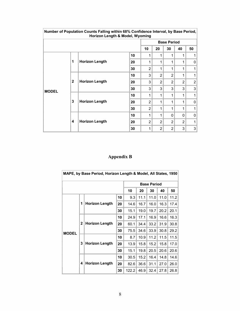
How similar are the results from one launch year to another? To answer this question, we

calculated the average errors and half-widths of the state forecasts for each of the three launch

years, by model, length of base period, and length of forecast horizon. The complete results can

be found in Appendix B; we summarize them here.

In every launch year and for every combination of model, base period, and forecast

horizon, MAPEs for Model 1 were very similar to those for Model 3. For the 1950 and 1960

launch years, MAPEs for Models 1 and 3 were almost always smaller than those for Models 2

and 4. For 1970, however, MAPEs for Models 2 and 4 were often smaller than those for Models

1 and 3, especially for longer base periods. In almost every instance, MAPEs increased with the

forecast horizon in all three launch years. In all launch years, increasing the length of the base

period had little effect on MAPEs for Models 1 and 3 but generally reduced MAPEs for Models

2 and 4.

For Models 1 and 3, MAPEs for 1950 and 1970 were similar to each other and were

consistently larger than MAPEs for 1960. For Models 2 and 4, however, MAPEs were generally

largest for 1950 and smallest for 1970. Differences among launch years were much larger for

Models 2 and 4 than for Models 1 and 3. The linear models thus displayed greater consistency

from one launch year to another than did the nonlinear models.

MALPEs varied considerably from one launch year to another. For Models 1 and 3,

MALPEs were negative for every combination of base period and forecast horizon for launch

years 1950 and 1970, but were positive for a number of combinations for 1960. For Models 2

12

and 4, MALPEs were positive for most base-horizon combinations for 1950 and 1960, but were

negative for a number of combinations for 1970. As has been noted before, bias appears to vary

substantially (and unpredictably) from one launch year to another (e.g., Smith and Sincich 1992).

Lengthening the base period did not have a consistent effect on the results, sometimes increasing

MALPEs and other times reducing them. Lengthening the forecast horizon generally (but not

always) exacerbated upward or downward biases.

In all three launch years, half-widths were similar for Models 1 and 3 for most base-

horizon combinations. In every combination, they were smaller (usually much smaller) than the

corresponding half-widths for Models 2 and 4. There was no consistent relationship between the

launch year and the size of the half-width: Sometimes they were largest for 1950, sometimes for

1960, and sometimes for 1970. For every combination of model, base period, and launch year,

half-widths increased monotonically with the length of the forecast horizon. In most

combinations of model, forecast horizon, and launch year, half-widths declined as the base

period increased.

In most instances, then, the results regarding the effects of differences in base period,

forecast horizon, and model on forecast errors and half-widths were about the same for each

individual launch year as they were when all launch years were lumped together. In many

instances, however, the values of the errors and half-widths themselves differed considerably

from one launch year to another.

A Test of Confidence Intervals

One of the primary motivations of the present research was to evaluate the usefulness of

confidence intervals as measures of uncertainty. Many different time series models can be

constructed using different base periods, launch years, and sets of assumptions; each model

implies a different set of confidence intervals for each forecast horizon. How well do the models

analyzed in this paper perform in terms of predicting the uncertainty of future population

growth?

One way to address this question to calculate the number of population counts falling

within the 68% confidence intervals associated with each set of forecasts analyzed in this study

(e.g., Cohen 1986). Table 5 shows the calculations for each combination of model, base period,

and forecast horizon for forecasts aggregated across all states and launch years. Each cell is

based on 12 forecasts (four states for each of three launch years). If the confidence intervals

13

provide reliable measures of uncertainty, they will encompass approximately eight of the 12 out-

of-sample population counts.

(Table 5 about here)

According to this criterion, the confidence intervals analyzed in this study generally did

not provide reliable measures of uncertainty. The intervals associated with Models 1 and 3 were

too narrow. In no set of forecasts did more than six of the 12 population counts fall within the

predicted interval; in some sets, only two or three fell within the predicted interval. In this study,

then, the two linear models consistently underestimated the uncertainty inherent in population

forecasts. For these models, differences in the length of the forecast horizon did not have much

effect on the number of counts falling within the predicted interval, but reducing the length of the

base period generally led to a larger number falling within the interval.

The confidence intervals associated with Model 2 were too wide. In every set of

forecasts, 10, 11, or all 12 counts fell within the predicted interval. This model consistently

overestimated the uncertainty inherent in population forecasts, especially for longer forecast

horizons.

Model 4 performed better than the other models. For 10-year horizons, between five and

seven forecasts fell within the predicted interval; for 20-year horizons, either eight or nine; and

for 30-year horizons, between eight and eleven. Since the number of counts falling within the

interval generally increased with the forecast horizon for both Models 2 and 4, the results suggest

that nonlinear models may produce confidence intervals that increase too rapidly as the forecast

horizon becomes longer.

CONCLUSIONS

Virtually all the published research on the development and use of time series models to

construct confidence intervals for population forecasts has focused on the national level, where

population change is more stable and predictable than it is at the subnational level. This

research, however, has not lead to a consensus regarding the best models to use for constructing

confidence intervals and generally has not considered the reliability of the resulting confidence

intervals as measures of uncertainty.

In this paper, we extended this research by developing time series models for states and

evaluating the accuracy of the resulting forecasts. Using four models and data for several states,

launch years, and base periods, we constructed 720 point forecasts and sets of confidence

intervals. We evaluated these forecasts by comparing them to population counts for the

14

corresponding target years. Although the evidence was not always clear-cut, a number of

distinct patterns emerged from this analysis. Based on this evidence and the results of other

studies, we have drawn the following tentative conclusions.

The two linear models produced forecasts that differed very little from each other,

leading to MAPEs, MALPEs, and half-widths that were much the same for both models. Similar

results have been reported previously (Alho 1991; Voss, et al. 1981). It appears that first-order

autoregressive and moving average terms do not have much impact on forecasts from linear time

series models.

For the linear models, 10 years of base data were generally sufficient to achieve—or at

least come close to—maximum forecast precision (i.e., the smallest MAPEs). This result was

found for every state and launch year, even for 20- and 30-year forecast horizons. Similar results

for simple extrapolation techniques have been reported before (Smith and Sincich 1990).

Although longer base periods may be desirable for other reasons, they do not appear to be

necessary for improving the precision of forecasts based on linear time series models.

For the nonlinear models, 10 years of base data were not sufficient to achieve—or even

come close to—maximum forecast precision. Rather, MAPEs declined as base periods

increased, albeit generally at a diminishing rate. Typically, the declines were greater for longer

horizons than shorter horizons. Although the linear models produced more precise forecasts than

the nonlinear models when the base periods were relatively short, their superiority diminished as

the base period increased.

Overall, the linear models had a negative bias and the nonlinear models had a positive

bias. However, this result was not found for every state and launch year. Given this finding and

the fact that bias has been found to vary considerably from one time period to another (e.g.,

Smith and Sincich 1988, 1992), we do not believe there is enough evidence to draw any general

conclusions regarding the bias inherent in different types of time series models. We note that

changes in the length of the base period had no consistent impact on bias, either for the linear or

nonlinear models. This result has also been reported before (Smith and Sincich 1990).

Nonlinear models produced forecasts with half-widths that were much larger than those

produced by linear models. This result was found for virtually all combinations of state, launch

year, base period, and forecast horizon. Based on the results shown in Table 5, it appears that

confidence intervals produced by linear models may often be too narrow and those produced by

15

the nonlinear models may often be too wide. The results for the nonlinear models, however,

were not as uniform as those for the linear models.

All of these conclusions must be viewed as tentative. Are the findings reported here

general characteristics of time series models or are they specific to the present study? Would the

results be the same for other states or launch years? What other models might be developed?

What other evaluation criteria might be applied? Further research is needed before we can

answer these questions and draw firm conclusions.

It is clear that confidence intervals based on time series models vary by state, launch

year, model specification, length of base period, and length of forecast horizon. That is, they are

conditional upon the choices made in developing a specific model for a specific forecast. Given

the evidence presented in this paper and the lack of clear decision rules for choosing appropriate

models and base periods, we are not convinced that—at this time—confidence intervals based on

time series models can provide a realistic indication of the degree of uncertainty associated with

state population forecasts. Furthermore, we doubt that it is appropriate to assess uncertainty

based on the results of a single model. We believe a great deal more empirical work must be

done before we can draw such conclusions. We hope the present study is a step in that direction.

16

END NOTES

1. ARIMA models based on time intervals of less than one year may also require seasonal components for p, d, and q. 2. A general guideline is that at least 50 observations are needed for identifying and estimating the parameters of ARIMA models (Box and Jenkins 1970; Meyler, Kenny, and Quinn 1998; Saboia 1974). 3. De Beer’s model is an ARIMA (0,0,1) because the net migration time series for the Netherlands did not require differencing to make it stationary.

Table 1. Population Growth Rates by Decade, 1900-2000:

Florida, Maine, Ohio, and Wyoming

State

1900-1910

1910-1920

1920-1930

1930-1940

1940-1950

1950-1960

1960-1970

1970-1980

1980-1990

1990-2000

Florida 42.6% 27.2% 52.9% 30.2% 46.7% 78.1% 37.9% 42.6% 32.4% 23.2%

Maine 7.2% 3.5% 3.8% 6.1% 8.0% 6.3% 2.9% 12.4% 9.3% 3.7%

Ohio 15.0% 21.2% 14.9% 4.0% 15.2% 22.0% 10.2% 0.7% 0.6% 4.6%

Wyoming 58.1% 34.0% 14.7% 10.6% 16.0% 14.1% 1.5% 41.1% -4.2% 8.8%

Table 2. All States and Launch Years: Mean Absolute Percentage Error (MAPE), by Model, Length of Base Period, and Length of Forecast Horizon

Base Period 10 20 30 40 50

10 9.2 9.9 9.9 9.9 10.1

20 13.7 14.8 14.8 15.1 15.81 Forecast Horizon

30 15.9 17.4 17.7 18.2 18.6

10 19.0 13.3 12.7 12.4 11.9


30 56.0 30.7 28.2 22.7 20.2

10 9.5 9.9 10.1 10.3 10.7


30 16.4 18.0 18.4 18.9 19.4

10 18.7 14.6 13.7 11.9 11.5

20 41.3 26.7 20.3 17.2 16.8

Model

4 Forecast Horizon

30 67.9 41.8 27.9 21.3 19.2

17

Table 3. All States and Launch Years: Mean Algebraic Percentage Error (MALPE), by Model, Length of Base Period, and Length of Forecast Horizon

Base Period 10 20 30 40 50

10 -3.6 -4.3 -5.4 -6.1 -6.3

20 -4.8 -6.0 -7.9 -9.1 -9.51 Forecast Horizon

30 -6.4 -7.7 -10.2 -11.8 -12.4

10 7.3 5.2 4.2 3.6 2.8


30 36.6 26.5 19.9 15.8 12.3

10 -3.6 -4.7 -6.0 -6.9 -7.2

20 -4.9 -6.4 -8.5 -9.8 -10.43 Forecast Horizon

30 -6.5 -8.2 -10.8 -12.5 -13.1

10 7.7 7.3 4.0 1.8 1.0

20 26.5 21.1 12.5 7.4 5.3

Model

4 Forecast Horizon

30 46.7 35.4 20.7 12.0 8.4

Table 4. All States and Launch Years: Average Half-Width of the 68% Confidence Interval, by Model, Length of Base Period, and Length of Forecast Horizon

Base Period 10 20 30 40 50

10 9.1 7.7 7.3 6.6 6.0


30 18.5 14.7 13.5 12.0 10.9

10 35.5 24.8 22.2 18.6 16.4


30 169.6 99.6 90.1 74.3 64.9

10 10.1 6.7 6.0 5.3 4.8


30 21.5 12.4 10.7 9.2 8.2

10 25.1 16.4 13.4 11.4 10.2

20 63.0 36.8 30.3 25.6 22.9

Model

4 Forecast Horizon

30 116.0 57.4 48.4 41.1 36.6

18

Table 5. All States and Launch Years: Number of Population Counts Falling within

68% Confidence Interval, by Model, Length of Base Period, and Length of Forecast Horizon

Base Period 10 20 30 40 50

10 6 5 6 5 4

20 5 3 5 4 21 Forecast Horizon

30 5 4 5 5 5

10 10 10 11 10 10


30 12 12 12 12 12

10 5 5 4 4 4


30 5 4 5 4 3

10 6 6 5 7 7

20 8 9 9 9 9

Model

4 Forecast Horizon

30 8 8 9 11 11

REFERENCES

Alho, Juha M. 1990. “Stochastic Methods in Population Forecasting.” International Journal of Forecasting 6: 521-530.

Alho, Juha M. and Bruce D. Spencer. 1997. “The Practical Specification of the Expected Error of Population Forecasts.” Journal of Official Statistics 13: 203-225.

Box, George and Gwilym Jenkins. 1976. Time Series Analysis: Forecasting and Control. San Francisco: Holden Day.

Cohen, Joel E. 1986. “Population Forecasts and Confidence Intervals for Sweden: A Comparison of Model-based and Empirical Approaches.” Demography 23: 105-126.

De Beer, Joop. 1993. “Forecast Intervals of Net Migration: The Case of the Netherlands.” Journal of Forecasting 12: 585-599.

Granger, Clive, W. 1989. Forecasting in Business and Economics, 2nd Edition. New York: Academic Press.

Keilman, Nico, Dinh Quang Pham, and Arve Hetland. 2002. Demographic Research 6: 409-453.

Lee, Ronald D. 1974. “Forecasting Births in Post-Transition Populations: Stochastic Renewal with Serially Correlated Fertility.” Journal of the American Statistical Association 69: 607-617.

____________. 1992. “Stochastic Demographic Forecasting.” International Journal of Forecasting 8: 315-327.

___________. 1999. “Probabilistic Approaches to Population Forecasting.” Pp. 156-190 in Frontiers of Population Forecasting, edited by Wolfgang Lutz, James W. Vaupel, and

19

Dennis A. Ahlburg. New York: Population Council. Supplement to Vol. 24 of Population and Development Review.

Lee, Ronald D. and Shripad Tuljapurkar. 1994. “Stochastic Population Forecasts for the United States: Beyond High, Medium, and Low.” Journal of the American Statistical Association 89: 1175-1189.

McCleary, Richard and Richard Hay, Jr. 1980. Applied Time Series for the Social Sciences. Beverly Hills: Sage Publications.

McNown, Robert and Andrei Rogers. 1989. “Forecasting Mortality: A Parameterized Time Series Approach.” Demography 26: 645-660.

Meyler, Aidan, Geoff Kenny, and Terry Quinn. 1998. Forecasting Irish Inflation Using ARIMA Models. Technical Paper 3/RT/98. Economic Analysis, Research, and Publication Department. Central Bank of Ireland.

Nelson, Charles. 1973. Applied Time Series Analysis for Managerial Forecasting. Holden Day: San Francisco.

Pflaumer, Peter. 1992. “Forecasting US Population Totals with the Box-Jenkins Approach.” International Journal of Forecasting 8: 329-338.

Saboia, Joao. 1974. “Modeling and Forecasting Populations by Time Series: The Swedish Case.” Demography 11: 483-492.

Sanderson, Warren C. 1995. “Predictability, Complexity, and Catastrophe in a Collapsible Model of Population, Development, and Environmental Interactions.” Mathematical Population Studies 5: 259-279.

Smith, Stanley K. and Terry Sincich. 1988. “Stability over Time in the Distribution of Population Forecast Errors.” Demography 25: 461-474.

_____________________________. 1990. “The Relationship between the Length of the Base Period and Population Forecast Errors.” Journal of the American Statistical Association 85: 367-375.

_____________________________. 1992. “Evaluating the Forecast Accuracy and Bias of Alternative Population Projections for States.” International Journal of Forecasting 8: 495-508.

U.S. Census Bureau. 1956. Estimates of the Population of States: 1900 to 1949. Current Population Reports, Series P-25, No. 139. (Released on the Internet February 1996.)

________________. 1965. Revised Estimates of the Population of States and Components of Population Change 1950 to 1960. Current Population Reports, Series P-25, No. 304. (Released on the Internet April 1995.)

________________. 1971. Preliminary Intercensal Estimates of States and Components of Population Change 1960 to 1970. Current Population Reports, Series P-25, No. 460. (Released on the Internet August 1996.)

________________. 1984. Intercensal Estimates of States and Components of Population Change 1970 to 1980. Current Population Reports, Series P-25, No. 957. (Released on the Internet February 1995.)

________________. 1993. Intercensal Estimates of States and Components of Population Change 1970 to 1980. Current Population Reports, Series P-25, No. 1106. (Released on the Internet August 1996.)

________________. 2002. Table CO-EST2001-12-0 - Series of Intercensal State Population Estimates: April 1, 1990 to April 1, 2000. (Released on the Internet April 2002.)

________________. 2003. Table NST-EST2003-01 - Annual Estimates of the Population for the United States and States, and for Puerto Rico: April 1, 2000 to July 1, 2003. (Released on the Internet December 2003.)

20

Voss, Paul R. and Balkrishna D. Kale. 1985. Refinements to Small-Area Population Projection Models: Results of a Test Based on 128 Wisconsin Communities. Paper presented at the annual meetings of the Population Association of America, Boston, MA.

Voss, Paul R., Charles D. Palit, Balkrishna D. Kale, and Henry C. Krebs. 1981. Forecasting State Populations Using ARIMA Time Series Techniques. Report prepared by the Wisconsin Department of Administration and the University of Wisconsin-Madison.

Appendix A

MAPE, by Base Period, Horizon Length & Model, Florida

Base Period

MODEL 10 20 30 40 50

10 12.1 14.3 17.2 18.6 19.5

20 18.1 23.9 28.6 31.3 33.1 1 Horizon Length

30 25.0 31.5 37.1 40.5 42.7

10 15.4 6.1 7.8 7.0 7.4

20 22.5 3.0 6.4 5.7 7.2 2 Horizon Length

30 32.8 5.5 8.3 10.1 9.9

10 13.2 14.6 18.0 20.4 22.0

20 18.3 24.2 29.2 32.7 35.2 3 Horizon Length

30 25.3 31.7 37.5 41.7 44.5

10 16.3 12.1 13.8 11.8 12.2

20 24.1 14.7 16.3 11.9 12.9 4 Horizon Length

30 34.0 21.0 19.7 14.0 14.5

MAPE, by Base Period, Horizon Length & Model, Ohio

Base Period

MODEL 10 20 30 40 50

10 6.8 9.0 7.3 6.5 6.6

20 13.9 17.7 14.3 12.3 12.41 Horizon Length

30 18.3 22.1 17.0 14.1 14.2

10 8.8 9.1 10.6 10.3 9.6

20 13.9 15.9 20.1 15.9 15.32 Horizon Length

30 17.0 19.7 29.4 19.3 19.2

10 7.2 9.2 7.3 6.4 6.4

20 14.6 17.9 14.4 12.3 12.33 Horizon Length

30 19.3 22.4 17.2 14.1 14.2

10 7.4 10.7 10.0 7.0 6.5

20 24.7 32.6 22.4 14.9 13.04 Horizon Length

30 50.8 61.1 37.2 24.9 22.2

MAPE, by Base Period, Horizon Length & Model, Maine

Base Period

MODEL 10 20 30 40 50

10 5.1 4.7 3.9 3.4 3.3

20 7.9 5.7 4.5 4.5 5.2 1 Horizon Length

30 7.7 4.9 5.3 6.6 7.5

10 17.4 11.7 10.0 10.5 9.6

20 41.6 21.4 19.2 18.7 16.6 2 Horizon Length

30 68.8 30.7 29.1 26.5 23.6

10 4.8 3.7 3.5 3.4 3.4

20 8.1 5.5 4.6 4.8 5.3 3 Horizon Length

30 8.3 6.3 6.8 8.0 8.6

10 18.3 13.3 9.9 10.3 9.8

20 44.5 26.1 18.9 18.5 17.1 4 Horizon Length

30 73.5 36.0 28.6 25.0 23.5

2

MAPE, by Base Period, Horizon Length & Model, Wyoming

Base Period

MODEL 10 20 30 40 50

10 12.9 11.8 11.1 11.1 10.9

20 14.9 11.8 11.7 12.2 12.7 1 Horizon Length

30 12.8 11.1 11.4 11.4 10.0

10 34.5 26.1 22.3 21.9 21.1

20 66.0 43.2 32.2 26.9 22.6 2 Horizon Length

30 105.5 66.9 45.9 35.0 27.9

10 12.7 12.2 11.5 11.1 10.9

20 14.1 11.6 11.4 12.3 12.7 3 Horizon Length

30 12.7 11.7 12.1 11.7 10.3

10 32.7 22.4 20.9 18.7 17.4

20 71.9 33.2 23.4 23.3 24.0 4 Horizon Length

30 113.1 49.1 26.3 21.4 16.8

MALPE, by Base Period, Horizon Length & Model, Florida

Base Period

MODEL 10 20 30 40 50

10 -10.3 -14.3 -17.2 -18.6 -19.5

20 -18.1 -23.9 -28.6 -31.3 -33.1 1 Horizon Length

30 -25.0 -31.5 -37.1 -40.5 -42.7

10 -0.3 -3.6 -4.6 -4.9 -5.4

20 0.7 -2.7 -4.9 -5.7 -7.2 2 Horizon Length

30 1.7 -1.9 -5.0 -6.3 -8.9

10 -10.4 -14.6 -18.0 -20.4 -22.0

20 -18.3 -24.2 -29.2 -32.7 -35.2 3 Horizon Length

30 -25.3 -31.7 -37.5 -41.7 -44.5

10 -8.4 -1.2 -5.9 -6.8 -7.7

20 -14.1 1.5 -7.4 -9.1 -11.0 4 Horizon Length

30 -17.8 4.6 -7.8 -10.2 -13.2

3

MALPE, by Base Period, Horizon Length & Model, Ohio

Base Period

MODEL 10 20 30 40 50

10 1.8 1.4 0.1 -0.5 -0.6

20 9.5 8.6 6.1 4.9 4.6 1 Horizon Length

30 18.3 16.6 12.9 11.2 10.7

10 -1.4 -1.2 -1.7 -1.8 -2.0

20 2.2 4.0 3.4 2.6 2.0 2 Horizon Length

30 5.5 10.4 9.5 7.9 6.7

10 2.2 1.6 0.2 -0.4 -0.6

20 10.3 8.9 6.3 5.0 4.6 3 Horizon Length

30 19.3 17.0 13.1 11.3 10.8

10 6.6 10.7 5.9 3.2 2.7

20 24.7 32.6 19.8 13.1 11.7 4 Horizon Length

30 50.8 61.1 37.2 24.9 22.2

MALPE, by Base Period, Horizon Length & Model, Maine

Base Period

MODEL 10 20 30 40 50

10 -1.0 0.1 0.1 -0.4 -0.8

20 -3.5 -2.0 -2.3 -3.3 -3.9 1 Horizon Length

30 -6.8 -4.9 -5.3 -6.6 -7.5

10 7.7 8.9 9.5 9.4 8.7

20 19.9 19.3 19.2 18.3 16.6 2 Horizon Length

30 33.6 30.7 29.1 26.5 23.6

10 -1.8 -0.9 -1.1 -1.6 -1.8

20 -4.7 -3.3 -3.7 -4.5 -5.0 3 Horizon Length

30 -8.3 -6.3 -6.8 -8.0 -8.6

10 8.3 7.7 9.2 9.0 8.6

20 23.3 16.9 18.9 17.4 16.5 4 Horizon Length

30 40.8 26.6 28.6 25.0 23.5

4

MALPE, by Base Period, Horizon Length & Model, Wyoming

Base Period

MODEL 10 20 30 40 50

10 -4.7 -4.4 -4.7 -4.8 -4.2

20 -7.2 -6.6 -6.8 -6.8 -5.6 1 Horizon Length

30 -12.2 -11.1 -11.4 -11.4 -10.0

10 23.2 16.7 13.5 11.7 10.1

20 66.0 43.2 32.2 26.9 22.6 2 Horizon Length

30 105.5 66.9 45.9 35.0 27.9

10 -4.6 -4.9 -5.2 -5.1 -4.5

20 -6.9 -7.2 -7.4 -7.1 -5.9 3 Horizon Length

30 -11.7 -11.7 -12.1 -11.7 -10.3

10 24.2 12.2 6.7 2.1 0.4

20 71.9 33.2 18.7 8.2 4.0 4 Horizon Length

30 113.1 49.1 24.7 8.2 1.0

Mean 68% Half-width, by Base Period, Horizon Length & Model, Florida

Base Period 10 20 30 40 50

10 8.6 7.8 8.2 8.5 8.3

20 12.3 10.9 11.6 12.3 12.3 1 Horizon Length

30 14.6 12.7 13.6 14.6 14.7

10 37.0 22.8 19.6 17.0 15.2

20 93.5 48.8 41.7 35.8 31.9 2 Horizon Length

30 162.5 71.9 61.4 52.4 46.8

10 7.4 6.5 6.4 6.2 5.8

20 10.3 8.8 8.6 8.3 7.9 3 Horizon Length

30 12.2 10.3 10.0 9.7 9.2

10 30.4 15.0 10.4 9.3 8.4

20 83.1 30.1 20.0 17.7 16.0

MODEL

4 Horizon Length

30 183.2 43.3 28.6 25.1 22.7

5

Mean 68% Half-width, by Base Period, Horizon Length & Model, Ohio

Base Period 10 20 30 40 50

10 7.0 6.5 6.0 5.4 4.7

20 10.9 9.8 8.8 7.8 6.8 1 Horizon Length

30 13.9 12.4 11.0 9.6 8.3

10 36.1 26.1 23.4 19.2 16.7

20 108.9 73.0 64.6 51.9 44.5 2 Horizon Length

30 212.2 134.4 120.9 94.3 80.0

10 6.2 5.8 5.3 4.6 4.1

20 9.6 8.7 7.8 6.6 5.8 3 Horizon Length

30 12.2 10.9 9.6 8.1 7.0

10 22.8 11.9 8.7 8.5 7.7

20 58.5 26.2 18.5 18.8 17.0

MODEL

4 Horizon Length

30 99.7 40.7 29.6 30.4 27.7

Mean 68% Half-width, by Base Period, Horizon Length & Model, Maine

Base Period 10 20 30 40 50

10 8.7 7.9 7.6 6.4 5.7

20 14.7 12.9 12.1 10.1 8.8 1 Horizon Length

30 19.8 16.9 15.7 12.9 11.2

10 32.4 25.4 23.1 19.1 16.7

20 90.3 65.6 59.2 48.3 41.7 2 Horizon Length

30 176.9 110.1 99.3 81.0 69.6

10 6.6 6.1 5.6 4.8 4.3

20 10.7 9.6 8.5 7.2 6.3 3 Horizon Length

30 14.2 12.5 10.9 9.1 8.0

10 22.2 20.9 21.6 18.2 16.0

20 55.6 52.7 54.9 45.9 40.0

MODEL

4 Horizon Length

30 97.7 87.5 91.9 77.2 66.7

6

Mean 68% Half-width, by Base Period, Horizon Length & Model, Wyoming

Base Period

MODEL 10 20 30 40 50

10 12.1 8.8 7.4 6.1 5.5

20 19.5 13.4 10.9 8.8 7.7 1 Horizon Length

30 25.6 16.9 13.6 10.8 9.3

10 36.4 25.0 22.7 19.1 17.2

20 82.4 55.1 51.4 44.0 39.6 2 Horizon Length

30 126.9 81.8 78.9 69.4 63.2

10 20.3 8.3 6.7 5.7 5.1

20 34.4 12.5 9.8 8.1 7.2 3 Horizon Length

30 47.5 15.9 12.2 9.9 8.6

10 24.8 17.6 13.0 9.7 8.9

20 55.0 38.3 28.0 20.1 18.5 4 Horizon Length

30 83.2 58.2 43.5 31.7 29.5

Number of Population Counts Falling within 68% Confidence Interval, by Base Period, Horizon Length & Model, Florida

Base Period 10 20 30 40 50

10 1 1 1 0 0

20 1 0 0 0 01 Horizon Length

30 0 0 0 0 0

10 3 3 3 3 3


30 3 3 3 3 3

10 1 1 0 0 0


30 0 0 0 0 0

10 2 2 1 2 2

20 3 2 2 2 2

MODEL

4 Horizon Length

30 3 2 2 2 2

7

Number of Population Counts Falling within 68% Confidence Interval, by Base Period, Horizon Length & Model, Ohio

Base Period 10 20 30 40 50

10 2 1 1 1 1


30 1 1 1 1 1

10 2 2 3 3 3


30 3 3 3 3 3

10 1 1 1 1 1


30 1 1 1 1 1

10 2 1 1 2 2

20 2 2 2 2 3

MODEL

4 Horizon Length

30 2 1 2 3 3

Number of Population Counts Falling within 68% Confidence Interval, by Base Period, Horizon Length & Model, Maine

Base Period 10 20 30 40 50

10 2 2 3 3 2


30 2 2 3 3 3

10 2 3 3 3 3


30 3 3 3 3 3

10 2 2 2 2 2


30 2 2 3 2 1

10 1 2 3 3 3

20 1 3 3 3 3

MODEL

4 Horizon Length

30 2 3 3 3 3

8

Number of Population Counts Falling within 68% Confidence Interval, by Base Period, Horizon Length & Model, Wyoming

Base Period 10 20 30 40 50

10 1 1 1 1 1


30 2 1 1 1 1

10 3 2 2 1 1


30 3 3 3 3 3

10 1 1 1 1 1


30 2 1 1 1 1

10 1 1 0 0 0

20 2 2 2 2 1

MODEL

4 Horizon Length

30 1 2 2 3 3

Appendix B

MAPE, by Base Period, Horizon Length & Model, All States, 1950

Base Period 10 20 30 40 50

10 9.3 11.1 11.0 11.0 11.2

20 14.6 16.7 16.0 16.3 17.4 1 Horizon Length

30 15.1 19.0 19.7 20.2 20.1

10 24.9 17.1 16.9 16.6 16.3

20 60.1 34.4 33.2 31.9 30.8 2 Horizon Length

30 75.5 34.6 33.9 30.8 29.2

10 8.7 10.9 11.2 11.5 11.5

20 13.9 15.8 15.2 15.8 17.0 3 Horizon Length

30 15.1 19.8 20.5 20.6 20.6

10 30.5 15.2 16.4 14.8 14.6

20 82.6 36.6 31.1 27.0 26.0

MODEL

4 Horizon Length

30 122.2 46.9 32.4 27.8 26.8

9


Base Period 10 20 30 40 50

10 5.6 6.1 5.8 5.9 6.1

20 10.0 11.4 12.0 13.0 13.6 1 Horizon Length

30 13.2 14.1 14.5 15.8 16.5

10 21.1 14.9 13.6 12.9 11.5

20 32.7 18.6 13.3 10.2 9.1 2 Horizon Length

30 67.4 40.6 28.4 21.3 20.6

10 6.4 5.8 5.8 6.1 6.7

20 10.1 12.0 12.9 14.0 14.7 3 Horizon Length

30 13.7 14.7 15.4 16.8 17.5

10 15.8 16.3 15.2 10.6 9.7

20 23.5 23.3 20.3 12.7 13.3

MODEL

4 Horizon Length

30 51.3 46.1 39.5 21.0 17.2


Base Period 10 20 30 40 50

10 12.8 12.6 12.9 12.7 12.9

20 16.6 16.2 16.3 16.1 16.5 1 Horizon Length

30 19.6 19.1 19.0 18.6 19.2

10 11.0 7.8 7.5 7.8 7.9

20 15.2 9.6 12.0 8.3 6.5 2 Horizon Length

30 25.2 16.9 22.1 16.1 10.7

10 13.3 12.9 13.2 13.5 13.9

20 17.2 16.6 16.6 16.8 17.4 3 Horizon Length

30 20.4 19.5 19.3 19.2 20.0

10 9.6 12.4 9.4 10.5 10.2

20 17.8 20.1 9.3 11.8 10.9

MODEL

4 Horizon Length

30 30.1 32.5 11.9 15.2 13.6

10

MALPE, by Base Period, Horizon Length & Model, Launch Year, 1950

Base Period 10 20 30 40 50

10 -7.6 -10.2 -10.5 -11.0 -11.0

20 -5.4 -10.0 -10.7 -11.2 -11.1 1 Horizon Length

30 -13.2 -19.0 -19.7 -20.2 -20.1

10 6.6 3.3 0.9 1.4 0.7

20 36.1 21.7 13.4 14.7 12.5 2 Horizon Length

30 47.9 23.2 9.1 11.8 8.2

10 -8.0 -10.8 -11.2 -11.5 -11.5

20 -6.0 -10.8 -11.5 -11.7 -11.6 3 Horizon Length

30 -13.8 -19.8 -20.5 -20.6 -20.6

10 12.0 5.1 0.8 -0.4 -1.1

20 54.0 26.7 14.3 11.4 9.6

MODEL

4 Horizon Length

30 83.3 34.6 13.5 9.7 7.3

MALPE, by Base Period, Horizon Length & Model, All States, 1960

Base Period 10 20 30 40 50

10 5.6 3.8 1.6 0.9 0.6

20 -0.6 -3.7 -7.7 -8.9 -9.6 1 Horizon Length

30 3.6 -0.4 -5.9 -7.5 -8.3

10 20.1 14.1 12.4 10.9 10.0

20 31.5 18.1 13.3 8.9 7.7 2 Horizon Length

30 62.9 39.5 28.4 19.4 18.1

10 6.4 3.4 0.8 -0.2 -0.7

20 0.4 -4.1 -8.4 -9.9 -10.6 3 Horizon Length

30 4.8 -0.8 -6.5 -8.4 -9.1

10 15.3 16.3 15.2 10.6 9.7

20 23.5 23.3 20.3 10.0 8.0

MODEL

4 Horizon Length

30 51.3 46.1 39.5 21.0 17.2

11

MALPE, by Base Period, Horizon Length & Model, All States, 1970

Base Period 10 20 30 40 50

10 -8.7 -6.5 -7.3 -8.2 -8.4

20 -8.4 -4.2 -5.3 -7.2 -7.8 1 Horizon Length

30 -9.7 -3.8 -5.1 -7.9 -8.7

10 -4.8 -1.9 -0.8 -1.5 -2.2

20 -1.1 8.0 10.8 8.0 5.3 2 Horizon Length

30 -1.2 16.9 22.1 16.1 10.7

10 -9.3 -6.7 -7.7 -9.0 -9.5

20 -9.1 -4.3 -5.6 -7.9 -8.8 3 Horizon Length

30 -10.5 -3.9 -5.3 -8.5 -9.6

10 -4.2 0.6 -4.0 -4.7 -5.5

20 1.9 13.3 2.9 0.8 -1.6

MODEL

4 Horizon Length

30 5.6 25.4 9.0 5.3 0.6

Mean 68% Half-width, by Base Period, Horizon Length & Model, All States, 1950

Base Period 10 20 30 40 50

10 15.0 9.1 7.2 6.4 5.8

20 23.5 13.8 10.7 9.3 8.3 1 Horizon Length

30 30.1 17.5 13.3 11.3 10.1

10 62.6 30.0 22.9 19.2 16.9

20 164.0 73.3 56.5 45.2 39.8 2 Horizon Length

30 285.4 121.5 97.6 73.9 65.0

10 13.6 8.0 6.2 5.6 5.0

20 20.8 11.9 9.0 7.9 7.0 3 Horizon Length

30 26.4 14.9 11.1 9.6 8.5

10 34.8 16.7 13.6 11.1 9.6

20 84.6 35.9 29.8 23.7 20.3

MODEL

4 Horizon Length

30 165.7 54.7 46.8 36.8 31.3

12


Base Period 10 20 30 40 50

10 7.0 8.8 7.8 6.9 6.4

20 10.8 13.1 11.7 10.2 9.4 1 Horizon Length

30 13.6 16.2 14.4 12.6 11.6

10 20.9 29.6 21.9 18.5 16.3

20 49.8 71.7 52.9 44.9 38.8 2 Horizon Length

30 83.3 115.6 85.9 74.6 63.2

10 12.4 7.4 6.1 5.3 4.9

20 20.8 10.7 8.8 7.5 6.8 3 Horizon Length

30 28.5 13.3 10.8 9.1 8.3

10 22.0 16.4 11.3 10.9 10.0

20 55.5 35.4 24.0 24.0 21.8

MODEL

4 Horizon Length

30 92.0 53.7 36.6 37.4 34.0


Base Period 10 20 30 40 50

10 5.3 5.3 6.8 6.5 6.0

20 8.8 8.3 10.1 9.7 8.9 1 Horizon Length

30 11.8 10.5 12.6 12.0 11.0

10 23.0 14.9 21.8 18.2 16.1

20 67.5 37.0 53.3 44.8 39.6 2 Horizon Length

30 140.2 61.5 86.9 74.3 66.4

10 4.5 4.7 5.7 5.1 4.6

20 7.2 7.1 8.3 7.3 6.5 3 Horizon Length

30 9.6 9.0 10.2 8.9 7.9

10 18.4 16.0 15.4 12.2 11.1

20 49.0 39.1 37.2 29.2 26.5

MODEL

4 Horizon Length

30 90.2 63.8 61.8 49.1 44.6

13

Number of Population Counts Falling within 68% Confidence Interval, by Base Period,

Horizon Length & Model, All States, 1950

Base Period 10 20 30 40 50

10 3 2 2 2 2


30 3 2 2 2 2

10 4 3 3 3 3


30 4 4 4 4 4

10 3 2 2 2 2


30 3 2 2 2 2

10 2 2 2 2 2

20 3 2 2 2 2

MODEL

4 Horizon Length

30 3 2 3 3 3

Number of Population Counts Falling within 68% Confidence Interval, by Base Period, Horizon Length & Model, All States, 1960

Base Period 10 20 30 40 50

10 3 3 3 2 2


30 2 2 2 2 2

10 3 4 4 3 3


30 4 4 4 4 4

10 2 3 2 2 2


30 2 2 2 2 1

10 2 2 1 3 3

20 3 3 3 4 3

MODEL

4 Horizon Length

30 2 2 2 4 4

14

Number of Population Counts Falling within 68% Confidence Interval, by Base Period,

Horizon Length & Model, All States, 1970

Base Period 10 20 30 40 50

10 0 0 1 1 0


30 0 0 1 1 1

10 3 3 4 4 4


30 4 4 4 4 4

10 0 0 0 0 0


30 0 0 1 0 0

10 2 2 2 2 2

20 2 4 4 3 4

MODEL

4 Horizon Length

30 3 4 4 4 4

confidence intervals for population forecasts: a case ... reports... · confidence intervals for...

Documents