Conference:

Assessing pathogen fate, transport and risk in natural and engineered water treatment

Banff Alberta, Canada September 26, 2012

Jeff D. Senders &

M. R. Collins University of New Hampshire

Department of Civil & Environmental Engineering Durham, NH USA

1

Acknowledgements

The USEPA and TACnet

Prof. J. P. Malley, Jr.

Prof. P. J. Ramsey

Kellen Sawyer

Damon Burt

Varouna Appiah

Durham NH DWTP Operators:

Wes and Brandon 2

Presentation Outline

I. Overview of slow-rate biofilters

(SRBFs) II. Problem statement III. Research objective &

hypotheses IV. Modeling depth filtration in

SRBFs V. Developing and evaluating a

phenomenological SRBF model

VI. Model calibration and validation VII. Application to multiple

organisms VIII. Conclusions

3

Slow-Rate Biofiltration Systems (SRBFs)

http://jhu.edu

http://megphed.gov.in/gallery/sustainsource/slides/sustain4.htm

http://geosciencewater.com

Slow Sand Filtration (SSF)

Riverbank Filtration (RBF) 4

Artificial Recharge Systems (ARS)

Winthrop, Maine SSF

Pawtuckaway State Park, NH

Problem Statement

Even though these robust SRBF systems are among the oldest drinking water treatment technologies in existence, no model

exists that accurately describes microbial removals within SRBFs.

• Depth filtration models predict microbial transport in

saturated granular media. Unfortunately, these models assume the media is clean solid spheres, uniform in size.

• Slow-rate biofilters (SRBFs) utilize non-uniform granular

media and deposited substances at the fluid/media interface to enhance filtration efficiency; however, current filtration models do not account for this removal mechanism.

5

Research Objective

Develop a model that can be used to predict E. coli removals for drinking water treatment

in SRBFs.

6

Source: http://healthierprograms.com

E. coli modeling parameters:

(treated as constants)

Density (ρp) = 1090 kg/m3 Diameter (dp) = 1 x 10-6 m

Working hypotheses in SRBF model

I: Depth filtration can be modeled by accounting for non-uniform media using a surface area per

unit volume (as) designation.

II: Cake filtration is governed by an interfacial ripening phenomenon that can be

qualified/quantified.

7

Modeling depth filtration

∂C/∂L = λC

Integrated:

C/Co = exp-(λL)

= filter coefficient or impediment modulus (Length-1) L = length or depth of filter C = concentration of colloid

Iwasaki, 1937

8

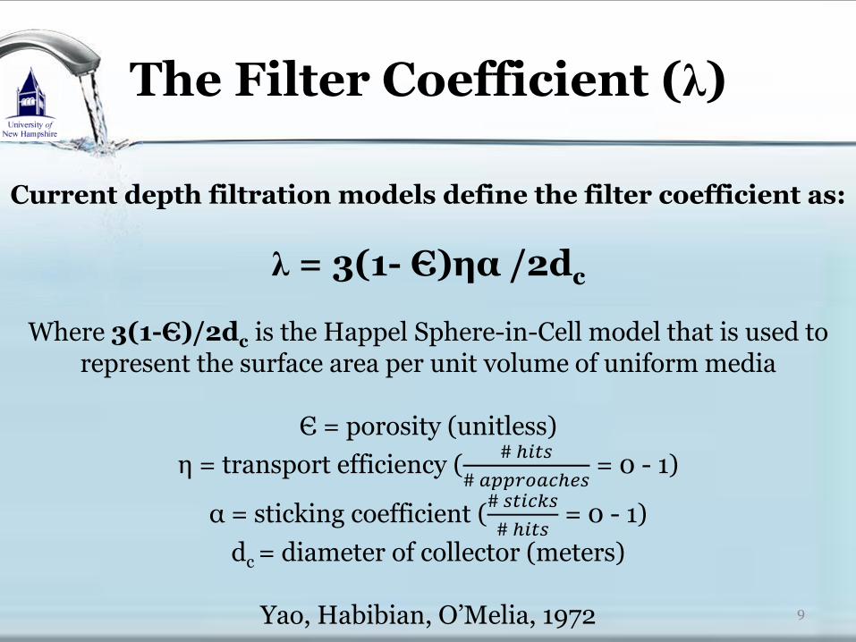
The Filter Coefficient (λ)

Current depth filtration models define the filter coefficient as:

λ = 3(1- Є)ηα /2dc

Where 3(1-Є)/2dc is the Happel Sphere-in-Cell model that is used to represent the surface area per unit volume of uniform media

Є = porosity (unitless)

η = transport efficiency (# ℎ𝑖𝑡𝑠

# 𝑎𝑝𝑝𝑟𝑜𝑎𝑐ℎ𝑒𝑠 = 0 - 1)

α = sticking coefficient (# 𝑠𝑡𝑖𝑐𝑘𝑠

# ℎ𝑖𝑡𝑠 = 0 - 1)

dc = diameter of collector (meters)

Yao, Habibian, O’Melia, 1972

9

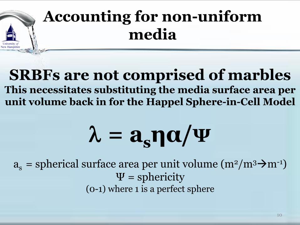
Accounting for non-uniform media

SRBFs are not comprised of marbles This necessitates substituting the media surface area per unit volume back in for the Happel Sphere-in-Cell Model

= asηα/Ψ

as = spherical surface area per unit volume (m2/m3m-1)

Ψ = sphericity (0-1) where 1 is a perfect sphere

10

Estimating the media surface area from a sieve analysis

Calculating the surface area per unit volume (as) from a standard sieve analysis

(Assuming the media is spheres of one size between two sieve pans)

as (meters-1) = [∑(# of grains di)( πdi2)]/[(∑ (# of grains di)( πdi

3/6))(Є/(1- Є) + 1)]

di = median diameter between two sieve sizes (meters) Є = media porosity

11

Comparison of media characteristics and hydraulic loading rate between SSF and RBF data sets

Parameter Units SSF RBF ASR

as m2/m3 6,446.92 10,388.79 9,207.45

das mm 0.53 0.38 0.41

d10 mm 0.32 0.14 0.20

d50 mm 0.57 0.65 0.65

UC d60/d10 2.03 5.93 4.25

Є 0.43 0.34 0.37

Ψ 0.84 0.84 0.84

HLR m/hr 0.175 0.045 0.074

0

10

20

30

40

50

60

70

80

90

100

0.01 0.1 1 10 100

% p

as

sin

g

D, mm

Particle Size Distributions of SRBF Media

RBF

SSF

ASR

dc as a function of as (das)

Total Unit Volume (Vt) = Void Volume (Vv) + Volume of Sand (Vs)

Vv = (Є/(1- Є))Vs Vt = (Є/(1- Є))Vs + Vs = Vs((Є/(1- Є)) + 1)

Substitute the volume of a sphere for the volume of sand (Vs)

Vt = πdas3/6((Є/(1- Є)) + 1)

Then the surface area per unit volume (as) may be expressed as

as = πdas2/ (πdas

3/6(Є/(1- Є)) + 1) = 6/das(Є/(1- Є) + 1)

Some algebra and a quick slide of hand

das= 6(1- Є)/as

12

The modified depth filtration model

C/Co = exp

-(asηαL/Ψ)

Within η, substitute dc for das.

das= 6(1- Є)/as

13

Do the modifications help us?

Pilot-scale SRBFs

Slow Sand Filters (SSF)

Riverbank Filter (RBF)

14

Artificial Recharge System (ARS)

The sticking coefficient (α) of pilot-scale SRBFs

15

Modified

The modified model reduces the sticking coefficient by an order of

magnitude and brings mathematical continuity to modeling with non-

uniform media.

α follows a power based trend that is a function of the empty

bed contact time (EBCT)

y = 0.6035x-1.074 R² = 0.8155

0.001

0.010

0.100

1.000

10.000

0 10 20 30 40 50 60

α

EBCT, hrs

α = -ψln(C/Co)/asηL

y = 2.8736x-1.074 R² = 0.8155

0.001

0.010

0.100

1.000

10.000

100.000

0 10 20 30 40 50 60

α

EBCT, hrs

α = -2dasln(C/Co)/3(1-Є)ηL

Traditional

Accounting for cake filtration

16

Changes observed in the sticking coefficient (α) are correlated to biomass, pH, and deposited substances.

0.001

0.010

0.100

1.000

10.000

100.000

1,000.000

0 5 10 15 20 25 30EBCT, hrs

α nmolPO43-/gdw10000[H+]CEC

17

In 1937, Tomihisa Iwasaki proposed a method to account for deposited

substances (specific deposit) that effect the filtration efficiency. He defined the impediment modulus (λ) with the following relationship:

𝝀 = 𝝀𝟎 + 𝒌𝝈 𝜎 = 𝑠𝑝𝑒𝑐𝑖𝑓𝑖𝑐 𝑑𝑒𝑝𝑜𝑠𝑖𝑡 𝑝𝑒𝑟 𝑏𝑒𝑑 𝑣𝑜𝑙𝑢𝑚𝑒 𝑖𝑛 𝑢𝑛𝑖𝑡𝑠 𝑜𝑓

𝑚𝑎𝑠𝑠

𝑣𝑜𝑙𝑢𝑚𝑒

𝑘 = 𝑟𝑎𝑡𝑒 𝑐𝑜𝑛𝑠𝑡𝑎𝑛𝑡 𝑒𝑓𝑓𝑒𝑐𝑡 𝑜𝑓 𝑠𝑝𝑒𝑐𝑖𝑓𝑖𝑐 𝑑𝑒𝑝𝑜𝑠𝑖𝑡 𝑤𝑖𝑡ℎ 𝑢𝑛𝑖𝑡𝑠 𝑜𝑓 𝜎−1𝑚𝑒𝑡𝑒𝑟𝑠−1

Defining the initial impediment modulus (i.e. depth filtration) as:

𝝀𝟎 =𝒂𝒔𝜼𝜶

𝚿

The proposed generic definition of the impediment modulus for SRBFs then becomes:

𝝀 =𝒂𝒔𝜼𝜶

𝚿+ 𝒌𝝈

Expanding the modified model to account for deposited cake substances:

Phenomenological SRBF Model

Developing a SRBF PhenMod

18

Acknowledging that multiple substances affect filtration efficiency, a generic

form of the impediment modulus can be defined as:

𝝀 = 𝝀𝟎 + 𝒌𝟏𝝈𝟏 + 𝒌𝟐𝝈𝟐 +⋯+ 𝒌𝒏𝝈𝒏

Through some calculus and selecting the concentration of hydrogen ions ([H+]), biomass (Bio), cation exchange capacity (CEC), metal oxides (Mox), and clay/silt (CS)

deposits as modeling parameters, this SRBF PhenMod may be expressed as:

lnC

C0= −

𝑎𝑠𝜂𝛼𝐿

Ψ+ 𝑢

𝑘[𝐻+] 𝜎𝐻+𝑑τ

𝜏

𝜏0+ 𝑘𝐵𝑖𝑜 𝜎𝐵𝑖𝑜𝑑τ

𝜏

𝜏0

+𝑘𝐶𝐸𝐶 𝜎𝐶𝐸𝐶𝑑τ

𝜏

𝜏0

+ 𝑘𝑀𝑜𝑥 𝜎𝑀𝑜𝑥𝑑τ

𝜏

𝜏0

+ 𝑘𝐶𝑆 𝜎𝐶𝑆𝑑τ

𝜏

𝜏0

Where: τ = residence time or empty bed contact time (EBCT, sec)

u = bulk fluid velocity or hydraulic loading rate (HLR, m/sec)

The initial SRBF PhenMod

19

Noting that the specific deposit follows a power-based trend that is a function of residence time or empty bed contact time (EBCT) of the

plug flow reactor, this Phenomenological SRBF Model integrates to:

𝑪

𝑪𝟎= 𝒆−(

𝒂𝒔𝜼𝜶𝑳Ψ

+𝒖𝑲𝒍𝒏𝝉)

τ = EBCT (seconds) u = HLR (m/second)

L (meters) K (meters-1)

A new unknown that might account for surface specific deposit characteristics-

a sight specific parameter.

Initial determination of K

20

Modeling Parameters

Average log removal difference: 0.4

Maximum over estimate: 1.9 log removal There is room for improvement…

1.E-05

1.E-04

1.E-03

1.E-02

1.E-01

1.E+00

0.0 0.5 1.0 1.5 2.0 2.5 3.0

C/C0

Depth, m

ASR 18C

ASR 23C

ASR 22C

ASR 18C obs

ASR 23C obs

ASR 22C obs

1.E-05

1.E-04

1.E-03

1.E-02

1.E-01

1.E+00

0.0 0.1 0.2 0.3 0.4 0.5 0.6 0.7 0.8 0.9 1.0

C/C0

Depth, m

U-SSF 17C

U-SSF 17C obs

1.E-06

1.E-05

1.E-04

1.E-03

1.E-02

1.E-01

1.E+00

0 1 2 3 4 5 6

C/C0

Depth, m

RBF 16C

RBF 17C

RBF 16C obs

RBF 17C obs

ASR RBF SSF Units

η 0.0246-0.0409 0.0167-0.0181 0.0064 N/A

α 0.005 0.005 0.005 N/A

u 0.050 0.074 0.193 m/hr

K 1.20E+04 1.20E+04 1.20E+04 m-1

Now what, calibration?

21

Bench-scale experiments were designed and executed for model calibration.

22

Bench-scale results for the rate constant K

Sums of Squares = 4.97 x 109 F Ratio = 88.35

R2adj = 0.57

𝑲 = −[𝟕. 𝟕𝟓 × 𝟏𝟎𝟒 + 𝟗. 𝟎𝟐 × 𝟏𝟎𝟑𝒍𝒏 𝑯𝑳𝑹 ]

Sums of Squares = 6.09 x 108 F Ratio = 127.38

R2adj = 0.66

HLR, m/s HLR, m/s 𝑲 = 𝒆(𝟗.𝟔𝟑−𝟏.𝟏𝟔×𝟏𝟎

𝟖𝑯𝑳𝑹𝟐)

Selected Regression

K K

Number of observations: 65

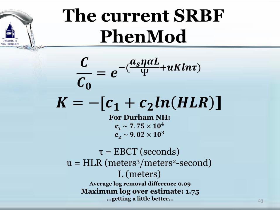
The current SRBF PhenMod

23

𝑪

𝑪𝟎= 𝒆−(

𝒂𝒔𝜼𝜶𝑳Ψ

+𝒖𝑲𝒍𝒏𝝉)

τ = EBCT (seconds) u = HLR (meters3/meters2-second)

L (meters)

𝑲 = −[𝒄𝟏 + 𝒄𝟐𝒍𝒏 𝑯𝑳𝑹 ]

Average log removal difference 0.09

Maximum log over estimate: 1.75 …getting a little better…

For Durham NH:

c1 ~ 𝟕. 𝟕𝟓 × 𝟏𝟎𝟒

c2 ~ 𝟗. 𝟎𝟐 × 𝟏𝟎𝟑

Application to multiple organisms

24

1.E-06

1.E-05

1.E-04

1.E-03

1.E-02

1.E-01

1.E+00

0.0 0.5 1.0 1.5 2.0 2.5 3.0

C/Co

Depth, m

Enterococci PhenMod Enterococci

Depth ModEnterococci

Enterococci obs

1.E-02

1.E-01

1.E+00

0.0 0.5 1.0 1.5 2.0 2.5 3.0 3.5 4.0 4.5 5.0

C/Co

Depth, m

Aerobic Spore Forming Bacteria (ASFB)

PhenMod ASFB

Depth Mod ASFB

1.E-02

1.E-01

1.E+00

0.0 0.5 1.0 1.5 2.0 2.5 3.0 3.5 4.0 4.5 5.0

C/Co

Depth, m

MS2

PhenMod MS2

Depth Mod MS2

MS2 obs1.E-05

1.E-04

1.E-03

1.E-02

1.E-01

1.E+00

0.00 0.25 0.50 0.75 1.00 1.25

C/Co

Depth, m

Bacillus 17.7C PhenMod11.5C PhenMod5C PhenMod5.5C PhenMod12.9C PhenMod21C PhenMod10.6C PhenMod5C PhenMod17.7C obs11.5C obs5C obs5.5C obs12.9C obs21C obs10.6C obs5C obs

Application to multiple organisms

25

𝑪

𝑪𝟎= 𝒆−(

𝒂𝒔𝜼𝜶𝑳Ψ

+𝒖𝑲𝒍𝒏𝝉)

𝑲 = −[𝒄𝟏 + 𝒄𝟐𝒍𝒏 𝑯𝑳𝑹 ]

Diameter (μm) Density (kg/m3) α c1 c2

1.00 1090 0.005 77500.00 9020.00 0.09 1.75

1.00 1090 0.200 15501.42 1803.91 -0.13 2.67

1.00 1090 0.003 15501.42 1803.91 0.06 0.49

0.50 1090 0.005 77500.00 9020.00 -0.37 -0.25

0.20 1090 0.0005 15501.42 1803.91 0.20 0.50

-0.03 1.03

0.22 1.17

Average log

removal

difference

Maximum log removal

over estimate

overall average

overall standard deviation

ASFB

MS2

SRBF Phenomenological Filtration Modeling Parameters

Enterococci

Organism

E. coli

Bacillus

Conclusions

26

Both cake and depth filtration must be accounted for when

modeling microbial removals in SRBFs.

This SRBF PhenMod is an inexpensive way to estimate microbial removals.

The efficacy of this model can help provide safe potable water to

impecunious regions around the world.

Current research is focusing on increasing model resolution by analyzing various substances within the cake filtration layer.

27

Thank You

Contact information Jeff D. Senders

447 Molyneaux Rd. Camden, ME 04843 USA sendersjeff@gmail.com

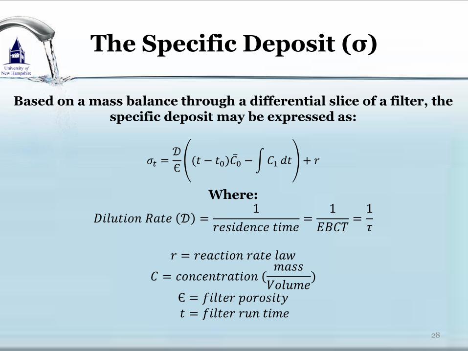
The Specific Deposit (σ)

28

Based on a mass balance through a differential slice of a filter, the specific deposit may be expressed as:

𝜎𝑡 =𝒟

Є(𝑡 − 𝑡0)𝐶 0 − 𝐶1 𝑑𝑡 + 𝑟

Where:

𝐷𝑖𝑙𝑢𝑡𝑖𝑜𝑛 𝑅𝑎𝑡𝑒 𝒟 =1

𝑟𝑒𝑠𝑖𝑑𝑒𝑛𝑐𝑒 𝑡𝑖𝑚𝑒=

1

𝐸𝐵𝐶𝑇=1

𝜏

𝑟 = 𝑟𝑒𝑎𝑐𝑡𝑖𝑜𝑛 𝑟𝑎𝑡𝑒 𝑙𝑎𝑤

𝐶 = 𝑐𝑜𝑛𝑐𝑒𝑛𝑡𝑟𝑎𝑡𝑖𝑜𝑛 (𝑚𝑎𝑠𝑠

𝑉𝑜𝑙𝑢𝑚𝑒)

Є = 𝑓𝑖𝑙𝑡𝑒𝑟 𝑝𝑜𝑟𝑜𝑠𝑖𝑡𝑦

𝑡 = 𝑓𝑖𝑙𝑡𝑒𝑟 𝑟𝑢𝑛 𝑡𝑖𝑚𝑒

Questions?

Experimental Approach

30

Phase I: An Interface Study 22 full factorial designed to evaluate the modeling parameters surface

area (as) and hydraulic loading rate (HLR)

*Also used for measurement systems analysis (MSA)

Phases II - IV: Further Assessment of the Interface

Phase II: 23 factorial experiment assessing clays, CEC, and BDOC

Phase III: HLR follow-up and further assessment of CEC and BDOC

Phase V: Validation Model validation using field observations

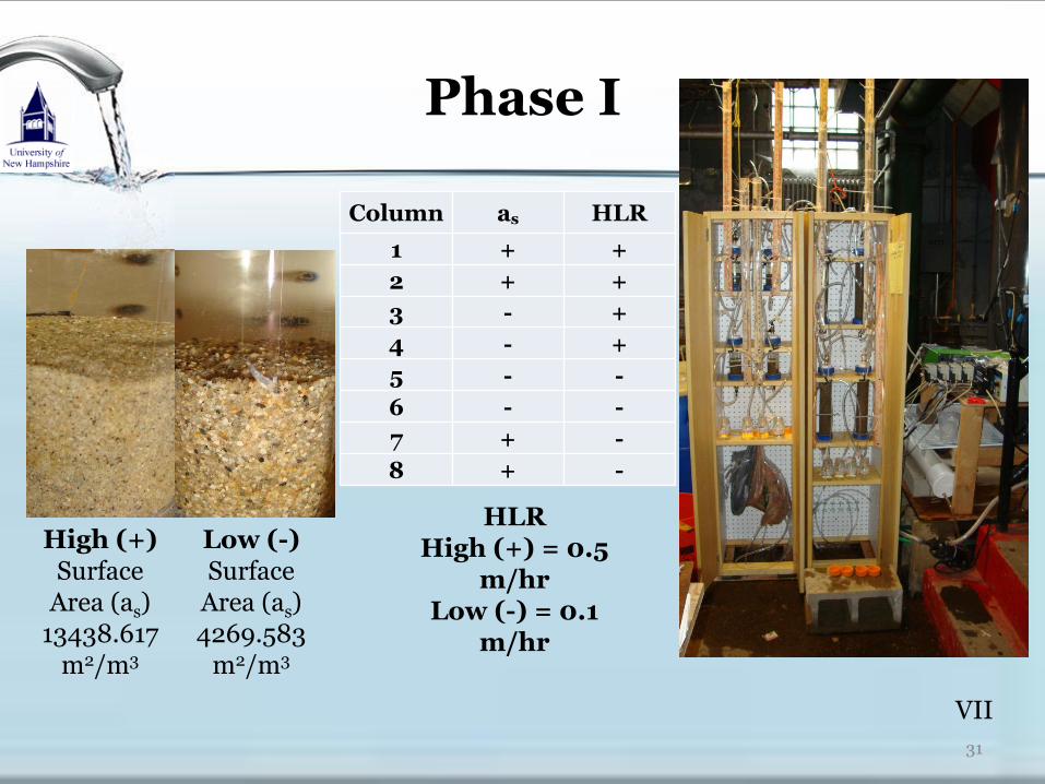
Phase I

31

VII

Column as HLR

1 + +

2 + +

3 - +

4 - +

5 - -

6 - -

7 + -

8 + -

High (+) Surface

Area (as) 13438.617

m2/m3

Low (-) Surface

Area (as) 4269.583

m2/m3

HLR High (+) = 0.5

m/hr Low (-) = 0.1

m/hr

Phase I Results

32

VII

Column As HLR

1 + +

2 + +

3 - +

4 - +

5 - -

6 - -

7 + -

8 + -

Phase I Results: HLR is Significant

33

VII

Column As HLR

1 + +

2 + +

3 - +

4 - +

5 - -

6 - -

7 + -

8 + -

Slow Sand Filtration (SSF)

Headspace

Supernatant Water

Schmutzdecke

Raw water

Filter drain & backfill

Sand media

Support gravel

Drain tile

Adjustable weir

Overflow weir

Vent

Control valve

Effluent Flow Control Structure

34

Comparison of Modeling With Different Diameters of SSF

Media

35

00.10.20.30.40.50.60.70.80.9

1

0 0.1 0.2 0.3 0.4 0.5 0.6 0.7 0.8 0.9 1

C/C

o

Depth, m

TE model predictions using differing diameters representative of

Winthrop media

d50

das

d10

da

dc

dg

dSB

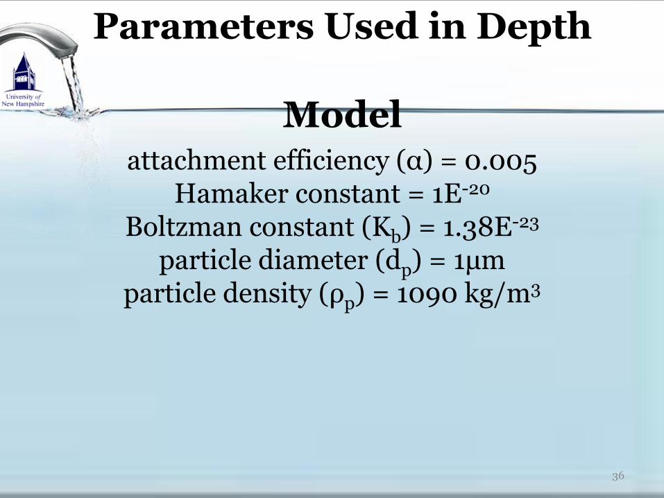
Parameters Used in Depth

Model

36

attachment efficiency (α) = 0.005 Hamaker constant = 1E-20

Boltzman constant (Kb) = 1.38E-23 particle diameter (dp) = 1μm

particle density (ρp) = 1090 kg/m3

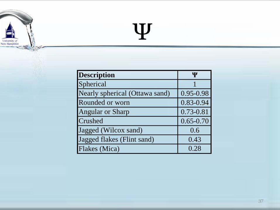
Ψ

37

Ψ

1

0.95-0.98

0.83-0.94

0.73-0.81

0.65-0.70

0.6

0.43

0.28

Crushed

Jagged (Wilcox sand)

Jagged flakes (Flint sand)

Flakes (Mica)

Description

Spherical

Nearly spherical (Ottawa sand)

Rounded or worn

Angular or Sharp

List of Terms

38

filter coefficient (Length-1

)

η total transport or single collector efficiency, dimensionless

α attachment efficiency or sticking coefficient, dimensionless

L depth of filter, meters

C particle concentration at depth L

Co initial particle concentration

as surface area per unit volume (Length-1

, m2/m

3)

Ψ sphericity (0-1)

Є porosity

γ porosity function, dimensionless

As porosity function, dimensionless

Pe Peclet number, dimensionless

dp diameter of particle, meters

ap radius of particle, meters

ρp density of particle (1090 kg/m3 used)

dc diameter of collector as a function of the Happel Cell, meters

ρc density of collector (sand: ρ = 2650 kg/m3)

Kb Boltzmann constant, 1.3805x10-23

J/K (kg*m2/s

2)

T absolute temperature, (oK= 273.15 +

oC)

vf fluid velocity (m/s)

vs Stoke’s settling velocity (m/s)

μ dynamic viscosity (kg/m*s)

g gravity (9.81 m/s2)

NLo London-van der Waals group, dimensionless

Ha Hamaker constant, 3x10-21

- 4x10-20

J (1x10-20

kg*m2/s

2 used)

Nr or R* relative-size group (dp/dc, dimensionless)

Ng transport efficiency due to gravity, dimensionless

di diameter of media retained in sieve #

at total surface area of sieve analysis (m2)

da arithmetic mean collector diameter

d10 effective size (10% passing by mass)

dsb sphere in box collector diameter

das surface area per volume collector diameter

dg geometric mean collector diameter

d50 50% passing by mass

d60 60% passing by mass

filter coefficient (Length-1

)

η total transport or single collector efficiency, dimensionless

α attachment efficiency or sticking coefficient, dimensionless

L depth of filter, meters

C particle concentration at depth L

Co initial particle concentration

as surface area per unit volume (Length-1

, m2/m

3)

Ψ sphericity (0-1)

Є porosity

γ porosity function, dimensionless

As porosity function, dimensionless

Pe Peclet number, dimensionless

dp diameter of particle, meters

ap radius of particle, meters

ρp density of particle (1090 kg/m3 used)

dc diameter of collector as a function of the Happel Cell, meters

ρc density of collector (sand: ρ = 2650 kg/m3)

Kb Boltzmann constant, 1.3805x10-23

J/K (kg*m2/s

2)

T absolute temperature, (oK= 273.15 +

oC)

vf fluid velocity (m/s)

vs Stoke’s settling velocity (m/s)

μ dynamic viscosity (kg/m*s)

g gravity (9.81 m/s2)

NLo London-van der Waals group, dimensionless

Ha Hamaker constant, 3x10-21

- 4x10-20

J (1x10-20

kg*m2/s

2 used)

Nr or R* relative-size group (dp/dc, dimensionless)

Ng transport efficiency due to gravity, dimensionless

di diameter of media retained in sieve #

at total surface area of sieve analysis (m2)

da arithmetic mean collector diameter

d10 effective size (10% passing by mass)

dsb sphere in box collector diameter

das surface area per volume collector diameter

dg geometric mean collector diameter

d50 50% passing by mass

d60 60% passing by mass

η is a function of a collector diameter (dc)

Differences in diameters used for modeling (d10, d50, d60,..etc.) in non-uniform media confounds comparisons

between researchers.

η = 2.4As1/3Nr

-0.081Pe-0.715NvdW

0.052

+ 0.55AsNr1.675NA

0.125 + 0.22Nr

-0.24Ng1.11NvdW

0.053 or

η = 4[2(1-γ5)/(2-3γ+3γ5-2γ6)]1/3(3μπvfdpdc/KbT)-2/3

+ [2(1-γ5)/(2-3γ+3γ5-2γ6)](4Ha/9πμdp2vf

1/8)(dp/dc)15/8

+ 3.38x10-3[2(1-γ5)/(2-3γ+3γ5-2γ6)](g(ρp-ρw)dp2/18μvf)

1.2(dp/dc)-0.4

Tufenkji & Elimelech, 2004

39

Rapid vs. Slow Rate Biofilters

Slow

40

Rapid

Filtration Mechanisms

Media Characteristics

Hydraulic Loading Rate (HLR)

Empty Bed Contact Time (EBCT)

5 – 30 m3/m2-hr

0.05 - 0.4 m3/m2-hr

Non-uniform UC > 2.5

Cake & Depth

Uniform UC < 2

Depth

Hours-days Minutes

But…

The Happel Sphere-in-Cell Model only applies to solid spheres uniform in size

3(1- Є)/2dc = as

as = surface area per unit volume (meters-1) dc = diameter of collector (meters)

Є = porosity (unitless)

John Happel, 1958

41

Accounting for cake filtration

Clay/silt deposits and higher natural organic matter

(NOM) removals in the upper region of SRBFs corresponds to viable biomass, and an increase in the cation exchange capacity (CEC). The increase in CEC

allows for greater retention of metal oxides and cations. This ripening phenomenon then relates to the enhanced

E. coli removals associated with SRBFs.

42