CPT AnalystVersion 6.2

1

QUICK START WITH DEMONSTRATION FILES

DownloadYou need to place all three files (CPT Analyst.CAB, Setup.EXE, Setup.LST) in a separate folder that you can find easily. These three files were sent to you a little earlier using the WhaleMail web site. All three of these files will need to be downloaded. Scroll lower in the email message to get all three of the files. Some places need administrator privileges to install a program on a computer. You will need to check with you network administrator if you have problems with installation. CPT Analyst.CAB is a compressed file with the CPT-Analyst.EXE and other subroutines necessary to run the program. With all three of the files discussed above in one folder, you are ready to being the installation

InstallationClick on the Start button followed by the Run. This will then bring up the Run dialog box. Click the Browse button and go to the directory that contains the files that were distributed for the programs. Click on the Setup program and then the click on the Okay button. This will begin the installation. At this point, simply answer the questions as to where you want to put the programs. It is recommended that you use the default directories.From the Windows Start menu, simply select the CPT-Analyst program and follow the instructions on the screen.

Running CPT-AnalystFrom Windows, click Start and then pick CPT-Analyst from the list of programs that you have installed on your system. The menu is set so that it generally follows the process of working on a project. The sequence to be used is as follows:

1. First, you will need to determine if you want to select layers manually or have the computer make a first cut at identifying the layers. Manual Layer Selection. From the Main Menu, Select Edit and then Edit

Minimum Thickness. Enter a 0 if you want to select the layers manually. When the screen later presents the graphs on the screen, simply place the cursor where you would like a layer and then left click. To delete a layer, move the cursor on top of the layer and left click.

Auto Layer Selection. From the Main Menu, select Edit and then Edit Minimum Thickness. If you enter anything greater than 0, the program will do a first cut of the possible layers. If you want 1 foot to be the thinnest layer, then enter about .8 feet and the program will select the layers using that criteria. You can experiment with this feature to determine your own preferences.

2. Next, you will need to give the program information on the files that contain the measurement data collected in the field. The correct information for reading the data must be entered in the Vendor and Project Data (VPD) file.

2

To begin with, simply use the Demo.VPD file that was provided with the program. Detailed information on the variables and data in this file are contained in Appendix A.

3. Once the VPD data file is selected, you will need to enter the name of the file that contains the soil behavior zones and the data that is associated with the behavior zones. This as a fairly large file and contains a lot of information. To begin with, use the Material8.MBD file that is supplied. Once you understand how the program works, this data can later be modified to meet your specific needs.

4. You will next be asked for the sounding file that contains the field measurements. The information telling the program where the information is contained data file is in the VPD file. If the data is read in correctly, the program will move on and graph the data and information your screen. Add and delete layers as desired in this screen.

5. With the sounding divided into layers, the layers identified and their empirical engineering parameters calculated, the data and information can be viewed, printed or cancelled. Simply click on the desired event. If you Save & Exit, the program will save the layer boundaries that you have and allow you to come back later and look at the same work at another time.

The DEMO files with the .CPT extension are only for demonstration purposes. If you don’t need them, you can delete them using Windows Explorer. It is not recommended that the sample control files (VPD, MBD) be deleted. You can later modify these files to meet the needs of your specific project and not have to build them from scratch.

3

LICENSE AGREEMENT

PrefaceCPT-Analyst and this user's manual are intended to provide practicing geotechnical engineers and engineering geologists with a relatively quick and easy-to-use means of performing data reduction and evaluating liquefaction potential.CPT-Analyst runs on a PC compatible computer with a Pentium processor using the WINDOWS 98 or newer operating system. The essential information needed to provide input and run the program is provided in this user's manual, with numerous paragraph headings to permit reference to specific topic areas.Any CPT-Analyst files may be copied only for legitimate archival or backup purposes for the end user who licensed the program. The CD may not be otherwise duplicated or redistributed in any form to any other party, under penalty of the U.S. copyright laws.Reference citations direct the user to additional information sources. Program assumptions and input-data limitations are explained to help the user determine the suitability of the programs to a particular situation.

AbstractThe CPT-Analyst Program is a WINDOWS compatible, interactive computer program. CPT-Analyst runs on a PC compatible computer with a Pentium processor having at least 64 mb of RAM using the WINDOWS 98 or newer operating system. The program is furnished as executable machine code (.EXE file) on a CD-ROM. CPT-Analyst accesses a CPT sounding file that can contain data for up to 2000 readings and create up to 200 layers. The program creates a report to the printer or disk-data files of tabulated output summaries and graphical plots of the output. A sample file data file and associate files than contain the material classification information are included for use with CPT-Analyst. These files can be modified and used at templates for future projects. In recognition of the potential for differing professional opinions and site specific data than can be developed for a project and what parameters should be assigned to different materials, instructions are given so that the user can generate his own material behavior-data file.

BackgroundThis software was initially developed in 1986 but was not widely distributed. However due to a increased interest and cone penetration test usage and the powerful interactive nature of the Windows Operating System, the software was adapted and update to the Windows environment. If you use the program, then it is only fair that you pay for it. This will also help support future improvements. If you have suggestions for improvements, then please send them to me. If you have a request for changes to the software to meet your specific needs, then an agreed price for making those changes can be worked out. However, if the changes are of a general nature that the program author deems marketable to others, then the changes may be incorporated in normal program updates.

4

End User RestrictionsNed Larson Software Company has granted, and the End User has accepted, upon the terms and conditions set forth herein, a personal nonexclusive license to use the Cone Penetrometer Software developed and owned by Ned Larson Software Company, hereinafter referred to as NLSC.The End User understands that NLSC would be damaged by unauthorized copying, duplication or distribution of the Cone Penetrometer Software and that those practices are prohibited under this agreement except to make archival copies of the Cone Penetrometer Software. The End User may not distribute, sublicense, copyright, or otherwise transfer this license without written consent from NLSC. One copy must be purchased for a given office/location and may be copied for use on multiple computers within that office. However, entities with more than one office/location must purchase copies of the Cone Penetrometer Software for each of the other offices/locations where the user wants to utilize the program.

Limited WarrantyCPT-Analyst, is a Computer Program for the data reduction and liquefaction analysis using the cone penetration test results, WINDOWS 98 and newer Compatible Versions, User's Manual. Copyright 1986-2004 by: Ned B. Larson11223 Minstrel Tune DriveGermantown, MD 20876(301) 916-7951 (voice)nblarson@comcast.netIMPORTANT! The materials are provided to you, the user, on the express condition that you agree to this software license agreement. By using the this program, you agree to the software license agreement provisions. If you do not agree with those provisions, return these materials to Ned Larson Software within three (3) days from receipt, for a refund. All rights reserved. The CPT-Analyst program, its related data files; and the CD on which they are contained (collectively referred to as "Licensed Software") are licensed to you, the end user, for your own use. You do not obtain title to the Licensed Software or any copyrights or proprietary rights in the Licensed Software. You may not sub-license, or disassemble the Licensed Software for any purpose. Reproduction or use of editorial or pictorial content in any manner without the express written permission of the author is prohibited. Although efforts have been made to accurately present the material, the Licensed Software is provided "as-is." No liability is assumed with respect to machine compatibility, program operation, output accuracy, or information contained herein. In no event will NLSC be liable for direct, indirect, special, or consequential damages including but not limited to any loss of business, interruption of service, loss of anticipatory profits, inability to use CPT-Analyst Software or the inability of CPT-Analyst Software to operate with or in conjunction with other products, even if they have been advised of the possibility of such damages. It is assumed that firms that purchase and use CPT-Analyst, and its related data files are familiar with the methods and procedures available for

5

interpreting CPT results, knowledgeable in the procedures for estimating earthquake liquefaction potential, and are qualified to correctly apply them in their design practices. It is the responsibility of the firms using this CPT-Analyst User's Manual and its related program, to verify their accuracy and suitability to a particular design application. The program author shall not be liable for any coincidental or consequential damages in connection with or arising out of furnishing or use of the program or this user's manual. The user accepts and uses this manual and its related program at his own risk, in reliance solely upon his own inspection of the material and without reliance upon any representation or description thereof. If the user detects errors or problems, it would be appreciated if they would be brought to the attention of the author, so that efforts can be made to correct future editions of the program. NLSC’s entire liability hereunder for damages, regardless of the form of action, will not exceed the charges paid by the End User to NLSC for this particular license.Because of the wide variety of sites where the cone penetrometer data may come from and the different uses of the data, the data files that are included only as examples and must be verified by a Professional Engineer to determine their suitability for a site and applicability for the analyses to be performed. NLSC makes no recommendation on the validity or completeness of any of the classification schemes discussed herein or the accuracy of the methods used to determine the different parameters.If the End User cannot live by this agreement, then return the software and you will receive a full refund.

SupportBecause of the limited market under which this software is sold, there is not sufficient volume to have full time support so I still have to work at another job. Much effort has been made to make the software as usable as possible with no support by providing example data files, plotting routines to visually check input parameters, and documentation. This is not a general-purpose computer program where usage can begin with only limited or no reading of the documentation. Instead this program is intended to solve a specific and specialized problem so the documentation and data files must be fully understood before beginning project work. Understanding the documentation and data files will minimized any problems you may encounter running the software. No support is implied or promised. However, you might be able to catch me in the evenings at 301-916-7951. If no one answers, then leave a message and I will get back to you. The best way to contact me is through email. I am out of town often so I may not respond immediately. My email address is nblarson@comcast.net.It is assumed that the End User is already experienced in the use and operation of Windows and reasonably familiar with the computer hardware. Because of my limited time, I cannot solve hardware-related problems.

6

MiscellaneousIf any applicable statute or rule or law invalidates any part of this agreement, the remainder of the agreement shall remain binding upon all parties. The laws of the state of Maryland shall govern this agreement.

TrademarksAll product names mentioned in this manual are trademarks of their producers.

7

Table of Contents

CPT Analyst........................................................................................................................... 1Version 6.1.................................................................................................................. 1

QUICK START WITH DEMONSTRATION FILES..........................................................................2INSTALLATION............................................................................................................. 2

LICENSE AGREEMENT............................................................................................................ 4Preface........................................................................................................................ 4Abstract....................................................................................................................... 4Background................................................................................................................. 4End User Restrictions...................................................................................................4Limited Warranty......................................................................................................... 5Support....................................................................................................................... 6Miscellaneous.............................................................................................................. 6Trademarks................................................................................................................. 6

Chapter 1: INTRODUCTION....................................................................................................9Background................................................................................................................. 9Program Implementation.............................................................................................9

Chapter 2: INSTALLATION & RUNNING THE PROGRAM.........................................................10Installation with Windows..........................................................................................10Running the Program.................................................................................................10Demonstration Files...................................................................................................11

Chapter 3: MAIN SCREEN....................................................................................................12Initial Menu Screen....................................................................................................12File 12

Open Vendor and Project Data (.VPD)..............................................................12Open Material Behavior Data (.MBD)................................................................13Open Cone Data files.......................................................................................14Graphics Printer and Report Printer Setup........................................................15

Edit 16Edit Minimum Thickness for Automatic Layer Selection....................................16Create/Edit VPD Data File.................................................................................17

View 19View Colors......................................................................................................19

Chapter 4: LAYER SELECTION SCREEN................................................................................20Layer Selection..........................................................................................................20Screen Information....................................................................................................21

Liquefaction Information..................................................................................21Depth 21Layer Number..................................................................................................21Depth Below Layer..........................................................................................21Data Point Information at Bottom of the Screen...............................................22Layer Information at the Bottom of the Screen................................................22

Material Behavior Plot for a Layer..............................................................................22Parameters Edited Directly on Screen........................................................................23

Pixels per Point................................................................................................23

8

Points Ignored.................................................................................................23Max Scale for First Plot....................................................................................24Max Scale for Second Plot................................................................................24Max Scale for Third Plot...................................................................................24Max Scale for Fourth Plot.................................................................................24Max Scale for Fifth Plot....................................................................................24

File 24Print Layer Report............................................................................................24Print Layer Graph............................................................................................25Print Layer Report and Graph..........................................................................25Save Layer Report File.....................................................................................25Save Layer Data File........................................................................................26Print Data Point Report....................................................................................26Print Data Point Graph.....................................................................................26Print Data Point Report and Graph...................................................................26Save Data Point Report File.............................................................................26Save Data Point Data File................................................................................26Save & Exit......................................................................................................26

Edit 26Magnitude.......................................................................................................27Acceleration.....................................................................................................27Water Depth for Liquefaction Analysis.............................................................27Water Depth during CPT for Normalization.......................................................28Fit Plot on a Single Page..................................................................................28Set feet per Page.............................................................................................28Select Parameters for Screen Layer Selection..................................................28Select Report Parameters................................................................................29Select Data File Parameters.............................................................................35Select Parameters for Material Behavior Zone Plot...........................................36

VIEW 36View Layer Report...........................................................................................36View Graph......................................................................................................37View Layer Data File........................................................................................38View Data Point Report....................................................................................38View Data Point Graph.....................................................................................39View Data Point Data File.................................................................................39

Clear Layers.............................................................................................................. 40Cancel....................................................................................................................... 40

Appendix A: DATA FILE FORMAT AND CONTENT..................................................................42Data File Layout.........................................................................................................42Vendor Parameter Data.............................................................................................42Material Behavior Type Data......................................................................................45LIQUEFY2................................................................................................................... 49REFERENCES.............................................................................................................51

9

CHAPTER 1: INTRODUCTION

BackgroundOne of the biggest benefits of using the cone penetrometer as a logging tool is that it can give a near continuous profile of soil conditions throughout the entire sounding. The disadvantage is that it can produce huge amounts of data that must be reduced and manipulated before it can be used and interpreted by an engineer. To date, the methods used to interpret the data have been widely varied. Solutions range from coarse visual interpretation to detailed processes using different computer programs that produce huge amounts of printouts.The method that is proposed using this computer code preserves the advantages of the CPT and by making the data interpretation easy. This program allows the engineer to quickly work with the CPT data and make decisions on how the profile is to be broken up into layers that can be used for further analysis. If the data are for a slope stability problem, then small weak layers are very important and the engineer may want to break them out for examination. If the data are to be used for a settlement analysis then the engineer may not want to break out layers that are quite thin to keep the amount of data needed for settlement analyses to reasonable amounts. This computer program allows the engineer quickly decide while allowing the computer to perform the tedious calculations necessary to use the CPT data as desired.

Program ImplementationThe program, as now implemented, is very simple and very interactive. It is based on a simple premise that one of my Professors used to say “If a picture is worth a thousand words, a graph is worth a million numbers.” The program is optimized to be very responsive for the interactive selection and editing of layers. This is done by plotting the sounding results on the screen using colors and symbols to convey a large amount of information to the user that can be quickly interpreted. This allows the engineer to efficiently perform his or her work and then move onto other tasks. Descriptions of the menu and what each option does are discussed later.

10

CHAPTER 2: INSTALLATION & RUNNING THE PROGRAM

Installation with WindowsFrom the Windows Start menu, simply select the CPT-Analyst program and follow the instructions.It is recommend that you create other subdirectories to hold the data files created for different projects. This way files can be easily managed and archived. Also the control files needed to run this program can be created or modified for a specific job and those files can then be stored with the raw data files from the different soundings. This way if there is a question in the future, all data will be present for examination.

Running the ProgramFrom Windows, click Start and then pick off CPT-Analyst from the list of programs that you have loaded on your system. The menu is set so that it generally follows the process of working on a project. The sequence to be used is as follows:

1. First, you will need to give the program information on the files that contain the raw measurement data collected in the field. The correct information for reading the data must be entered in the Vendor Property Data (VPD) file to read the data correctly. To begin with, simply use the VPD file that was provided with the program. Information on the variables and data contained in this file are contained in Appendix A of this manual.

2. Once the VPD data file is selected, you will need to enter the name of the file that contains the soil behavior zones and the data that is associated with the behavior zones. This as a fairly large file and contains a lot of information. To begin with, use the one that is supplied. Once you understand how the program works, this data can later be modified to meet your specific needs.

3. You will next be asked for the sounding file that contains the field measurements. The information telling the program where is find the correct information is contained in the VPD file. If the data is read in correctly, the program will move on and graph the data and information your screen. Manual Layer Selection. To select a layer, simply left click the mouse and

the program will calculate the average values and plot them on the screen. To delete a layer selection, simply move the cursor over the top of the layer and left click and the layer will de deleted.

Auto Layer Selection. From the Main Menu, select Edit and then Edit Minimum thickness. If you enter anything greater than 0, the program will do a first cut of the possible layers. If you enter 0, then no layer selection will be performed

4. With the sounding divided into layers, the results of the layers identified and their empirical engineering parameters can be viewed, printed or cancelled. Simply click on the desired event. If you Save & Exit, the program will save the layer boundaries that you have and allow you to come back later and look at the same work.

11

When you exit the CONE program, it will save the names of the files that you are using and then return control to Windows.

Demonstration FilesThe files that have DEMO in the file name are only for demonstration purposes. If you don’t need them then you can delete them using the windows Explorer. It is not recommended that the sample control files (VPD & MBD) be deleted. You can generally modify these files to meet the needs of your specific project and not have to build them from scratch.

12

CHAPTER 3: MAIN SCREEN

Initial Menu ScreenAt startup, Figure 3.1 is what you will see. Below is a description of what each of the menu options will accomplish.

Figure 3.1 Main Menu Screen

FileThis menu has the following sub items:

Open Vendor and Project Data (.VPD) This allows you to select a file that contains the information needed by the program to read raw data files supplied by the different vendors and to enter data and information that is specific to a project. See Appendix A for a more detailed description of the information needed in this file. This data file must use the “.VPD” extension in its name. The program will look for all files in the directory that have the VPD extension and the file names will be displayed in the box. Follow the instructions on the computer screen to select the file you want to use. Select a file by pressing the regular Windows commands.

13

Because of the wide variety of data format types, information describing the vendor’s data file is needed. This option will take a data file from a vendor, put it on the screen and allow you to make sure the layout is correctly reflected by the information in the vendor parameter data (VPD) file. If the parameters in the VPD file need to be modified, this option will also allow you to make these changes and then save them. If you are using a new vendor and don’t have a vendor parameter data file for the new vendor, simply use one of the existing VPD files, modify it to match the new vendor data that you have. If you have modified the data file, save it with the name of the new vendor (see the Appendix A for more information on the information stored in the VPD file). By modifying information in the VPD file, the program can read many types of file formats ranging from comma, space, or tab delimited records to fixed field formats where the numbers are stored in specific columns. Only one VPD file needs to be created for a group of files that have the same data file layout.Example VPD files are included for different vendors of CPT services. Some file formats may change with time so you will need to check the included VPD files against you actual data.

Open Material Behavior Data (.MBD) This option allows you to identify the name of the file that contains the material behavior zone information needed to classify the sounding data. The method included in this demonstration data file is taken from work done by Peter Robertson (1990) and is shown in Figure 3-2. Instructions for modifying one of these classification schemes or creating your own are discussed in Appendix A (see Appendix A for more information on the format of this data file). This data file must use the “.MBD” extension in its file name. Once this data file is identified, it will be used throughout a session unless changed through this option.The program will look for all files in the directory that have the MBD extension and the file names will be displayed in the box on the computer screen. Follow the instructions on the computer screen to select the file you want to use. Select a file by pressing the <Enter> key while the file name is highlighted or double click on the file you want to select. If you are selecting the file to be used from the list, you may type the first letter of the file name and that file will be highlighted. When there are multiple files with the same first letter then type the first letter of the file name again until the one that you want is highlighted. The lower portion of this data file contains the soil property data for each material behavior type zone and is needed to calculate the indicators and parameters for the selected layers. See Appendix A for more information on the format of this data file

14

Figure 3-2, Material behavior classification zones proposed by Robertson (1990).

Open Cone Data files As the data file is being read, the program will look for several indicators that signal the end of the file being imported has been encountered. These-end-of file indicators vary from vendor to vendor so making sure that every option is included is difficult. However, the following are checked and if encountered, importing will stop:1. End of file is encountered (^Z or control Z)2. If a value greater than or less than 20,000 is encountered in any of the columns.3. If one of the following characters are found in a data column: a, e, I, o, u, !, @, #, $, %, ^, &, *, (, ), _, +, =, |, \, {, }, [, ], <, >, ?, and /.

Because of the wide range of conditions under which the cone penetrometer is used, a value of 0 in the point stress, sleeve stress, or pore pressure is not

15

considered to be end-of-file indicator. A sounding file can contain no more than 3000 data points. Any reading that had a depth of 0 or the same depth reading of the previous point will simply be ignored and skipped overOnce the files have been read, the program will plot the data on the screen for layer selection.

Graphics Printer and Report Printer Setup In some instances, the graphics may need to be sent to a color printer and the report may be sent to a black and white printer, this will allow you to select a different printer for each.

16

EditThe Edit screen from the Main Menu is shown if Figure 3-3.

Figure 3-3 Edit Screen in the Main Menu

Edit Minimum Thickness for Automatic Layer Selection The program provides a method where it will go through the data file and select possible layers for analysis. If you are looking for small layers, then enter a small value and the program will automatically select layers based on that value. Typically this number would be a little smaller than the thinnest layer that you desire. For instance, if the minimum layer thickness that you would like, enter a 0.7 or 0.8. There may be a few layers slightly less than one foot but it most would be near one foot or larger. If a sounding contains a lot of thin layers, then the program has difficulty identifying the layers. If the layers are fairly thick, then the program does a better job selecting the layers. An Engineer or Geologist should check the layers identified by the program using the Layer Selection screen. Therefore, even though the program will make the first cut at identifying the layers, the user should go in and check the layers selected and make adjustments as necessary.If the ground water depth for liquefaction analysis is within the sounding, the

17

program will automatically insert a layer boundary at that depth, even if it is the same material. This is done so when the settlement analysis for liquefaction is calculated, the ground water depth for liquefaction is the break from dry sand settlement to liquefaction settlement.If you do not want the program to make a first cut at the layer selection, simply add a 0 for this value.

Create/Edit VPD Data File More data and information on the format of the VPD data file is contained in Appendix A. Because of the importance of this file, a screen view of the data file to make sure that you can edit the data and information for another file. An example of this would be when you receive data from another vendor, you would take an existing VPD data file, compare it to the VPD file that you currently have and then make the necessary adjustments. After you make the changes, it should be saved with a different name.

In using this option, the first question that the program will ask for is the name of a typical data file from the new vendor or project. The program will read the first 10 lines of the program and then place them in the box at the top of the screen. At the bottom of the box is the number of the columns of data that the program found. You will need to enter this data into the boxes below the data window so the program can find the data that it needs to work. See Appendix A for more information on which each of the data boxes represent.

The VPD file is a project specific file since it contains information like the title, earth quake information, ground water information and such. It is small so it doesn’t take much space if it is duplicated into multiple directories. The material behavior data file is large and is generally the same from project to project.Figure 3-4 shows what the screen looks like to edit/create the VPD data file. The user should be very careful to ensure that the right information is entered in the correct box. Most problems encountered in running the program are a result of not getting the right information into the VPD file.

Using the label information from the data fileFor the project title, the project number, the project identification, the CPT data and time, the cone/rig number, and the sounding number, the user has an option of which to use. Information can be used from the data file or it can be entered directly at this point. To use the information from that data file, the user will need to tell the CPT Analyst where to find that information in the data file. This is done by first entering an & in the first position in the text box. This signals to the program that location information for the data will follow. Next, simply add the line number followed by the beginning column and the ending column for the data and information. Once this is entered, simply click the “See Location Results” button and the program will get the information from the file

18

based on the location data that you have entered. The information in the shaded boxes will be used by the program in the printouts and labeling rather than that location information with the white background.

Entering the label information and by passing the information in the data fileIf you don’t want to use information in the data file, simply type the information that you would like to use in each of the text boxes. This information will over ride any thing that is contained in the CPT data files. If you hit the “See Location Results” button, it will take the information that you have entered and put it in the shaded boxes. As discussed above, the information shown in the shaded areas is what the program uses for printouts and labeling.

Figure 3.4 Main Menu Edit Screen for Create/Edit VPD Files.

All these parameters need to be carefuly filled out. Most problems in operating the program occur from not filling out these parameters correctly.

After a VPD file is edited for another project, simply hit the Save & Exit key. You will be prompted at that point if you want to save the information over the top of the existing file or create a new file.

19

ViewThe primary purpose of the View menu is to allow the user to plot the data and information that is entered in the MBD file. Figure 3-5 shows the choices from the Main Menu, View Screen. By plotting the information on the screen, the user can quick check to see if the data has been entered correctly in the file.

Figure 3-5 Main Menu View Screen

View Colors The colors that are used for the different material type polygons are identified using the combination of numbers for the red, green and blue. Each number can go up to 255. However, it is difficult to visualize the result from looking at the different numbers. This will allow the user to enter the color numbers in the computer and view the resulting color. Currently, this will not change the color numbers in the data file. The user will have to generate the colors, write them down, and then enter them in the MBD file using a text editor such as Notepad.

20

CHAPTER 4: LAYER SELECTION SCREEN

Layer SelectionThis option will allow the viewing of the results of the sounding data file and then allow the selection and editing of different layers. If you want the program to automatically select the layers then see the Main Screen, Edit, Edit Minimum Thickness that was discussed earlier.

Action CommandAdd Layer Boundary Left ClickDelete Layer Boundary Move cursor over the top of boundary and

left clickView layer data on Material Behavior Zone plot

Move cursor to layer and right click

Label a range of layers with a geologic/soil description (i.e. loose fill, etc.).

Move the cursor to the bottom layer of the range and shift-right click. A menu of the descriptions and the layer range will be presented. This should be done after all the layers have been selected. If you want a different description, you will need to go to the MBD file and add the description as desired. See Appendix A for the MBD file layout.

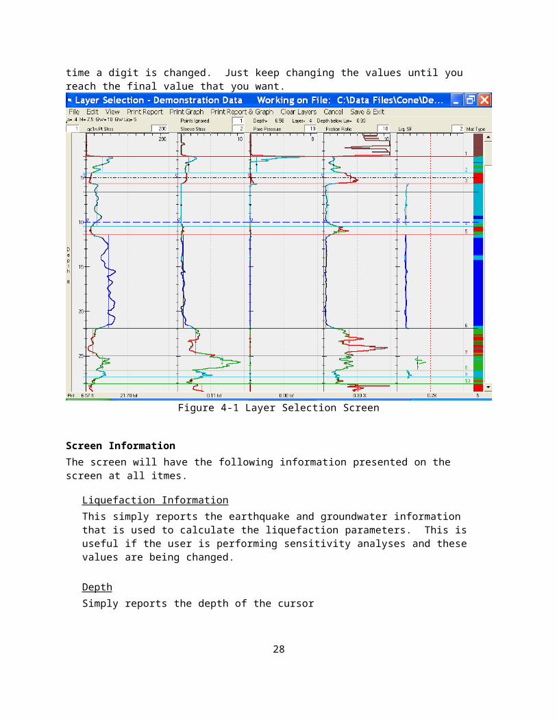
When a file is read, the program will present a screen similar to the one shown in Figure 4-1.

You now have the ability to do numerous sensitivity analyses on the data. Anytime one of the parameters such as the earthquake acceleration, earthquake magnitude or depth to groundwater, the program will re-calculate the all the information and reclassify the data if necessary and then re-plot the results on the screen.

The values in the text boxes at the top of the screen can be changed as desired. When a change is made, the program will automatically modify the screen to reflect the change. It is not necessary to hit the Enter key after the change is made. However, if you the change that you are making involves modifying multiple digits simply keep making the changes in the text box and the screen will change each time a digit is changed. Just keep changing the values until you reach the final value that you want.

21

Figure 4-1 Layer Selection Screen

Screen InformationThe screen will have the following information presented on the screen at all itmes.

Liquefaction Information This simply reports the earthquake and groundwater information that is used to calculate the liquefaction parameters. This is useful if the user is performing sensitivity analyses and these values are being changed.

Depth Simply reports the depth of the cursor

Layer Number When selecting layers, the program will report the layer number where the cursor is located.

22

Depth Below Layer This simply reports the depth that the cursor is below the previous layer boundary. When information is desired on the layer thickness, by putting the cursor on the lower layer boundary, the Depth Below Layer will report that layer thickness. When the user is manually selecting layers, this is especially useful to see that very thin layers are not selected.

Data Point Information at Bottom of the Screen At the bottom of the page, the actual data point values are printed. These values represent the actual data point that is closest to where the cursor is located. The depth value for the point will often be different from the depth value shown at the top of the page. The depth information shown at the top of the page is an interpolation between the pixels and the location of the line while the information at the bottom represents the nearest data point depth value.

Layer Information at the Bottom of the Screen When a layer is selected, the average values for the layer are plotted and the actual calculated values are printed at the bottom of the page. Because these represent the average values for the layer, they will not change until the cursor is moved to another layer. The left most number on the line under the data point depth is the thickness of the layer.

Material Behavior Plot for a LayerWhen a layer is selected by the computer or by the user, the user can check to see the within layer variability of the data points. By right clicking, all the data points in that layer are plotted on the friction ratio vs. point stress plot, which also shows the material zone polygons. This allows the user to see where the data in the layer is falling and the layer number is plotted for the average friction ratio and point stress. Figure 4-2 shows what this might look like. It should be noted that the percentages shown and the Normally Consolidated zone can be eliminated by selecting Edit, Select Parameters for Material Behavior Plots from the Layer Selection screen that is discussed a little later.

23

Figure 4-2 Layer data shown when the mouse is right clicked in the Layer Selection Screen

Parameters Edited Directly on ScreenThe following items can be changed directly from this screen by typing data and information directly into the boxes.

Pixels per Point This is the text box in the upper left portion of the screen. The program will currently plot a pixel for every point. A value of one is typically adequate for soundings where readings are taken every two inches or less. However, if the plot looks squashed and too small, simply increase the number of pixels per data point. Although it stretches out the graph in the depth direction, it does not truly add to the accuracy when the graph it stretched out using a large number of pixels per point.

Points Ignored As a sounding transitions from one material behavior type to another, sometimes the transition can look like it occurs over a depth but in reality, it could be a function of the cone configuration. When the average values of the

24

layers are determined, they could include the information that is not truly representative of the material behavior type. Therefore, this allows the user to eliminate points that could be considered part of the layer transition. For thick layers, this isn’t significant. However, for thin layers, this could have a large impact. If the layer is thin and the distance of the points ignored is more than the layer thickness, the program will take the reading at the center of the layer. Right clicking in a layer will plot the data that is used to determine the average values. When the average values are plotted for the layer. The average lines will extend only over the data that is used to determine the average values.

Max Scale for First Plot Sets the scale of the first plot. When this value is set, it is also used when a hard copy of the plot is produced.

Max Scale for Second Plot Sets the scale of the second plot. When this value is set, it is also used when a hard copy of the plot is produced.

Max Scale for Third Plot Sets the scale of the third plot. When this value is set, it is also used when a hard copy of the plot is produced.

Max Scale for Fourth Plot Sets the scale of the fourth plot. When this value is set, it is also used when a hard copy of the plot is produced.

Max Scale for Fifth Plot Sets the scale of the fifth plot. When this value is set, it is also used when a hard copy of the plot is produced.

When a file has been previously worked on and the layers selected, a data file will be created which stores the layer information using the root file name, but adds the “.OTX” extension to it. Each time a file name is entered to select the soil layers, the program will first check to see if the sounding data file exists and whether a file also exists with that same name but has an OTX extension. If it does, then it will load the sounding data file and the OTX data file so, that previous layer selections and edits can be maintained and/or modified. When a file with the OTX extension exists, all the soil layers will appear on the screen as they existed when the layers were selected the last time the file was worked on.

FileThe program will produce data in two general formats. One is simply allowing the

25

user to present and print the raw data from the sounding. This is always referred to as the Data Point Report, Graph, ets. The second allows the used to select a series of layers for design purposed. This is referred to as the Layer report, Graph, etc.

Print Layer Report When the parameters have been selected in the Edit, Select Layer Report Parameters, you can select this option to send the layer material directly to the printer.

Figure 4-3 View Layer Data from the Layer Selection ScreenIf the user wants to look at the individual data points that are part of a layer, simply highlight the layer and click on the Show Data button. This will then list all the individual data points that were measured in that layer.If the user would like to see all the layers plotted on one chart, simply click on the Select All and all the data for the layers selected will be plotted.

Print Layer Graph When the parameters have been selected in the Edit, Select Layer Parameters for Layer Paper Plots, you can select this option to send the charts directly to the printer.

26

Print Layer Report and Graph This will simply send the layer report and layer graphs discuss above to the printer

Save Layer Report File If you don’t want to send the layer report to the printer and want to create a data file instead, use this option. The file extension is set in the Edit menu when you select the parameters that are to be included in the report.

Save Layer Data File If you would like to create a data file that may be used by another program, this is the option that you would use. First you select the parameters that you want included in the data file using the Edit menu item. Once the parameters are selected, then use this command to save the file. This command differs from above in that this one will not include the headings of the different column in the data file.

The following commands are focused on the data point interpretation. These commands are focused on the data points rather than on the layers and results of the layers.

Print Data Point Report When the parameters have been selected in the Edit, Select Date Point Report Parameters, you can select this option to send the layer material directly to the printer.

Print Data Point Graph When the parameters have been selected in the Edit, Select Data Point Parameters for Data Point Paper Plots, you can select this option to send the charts directly to the printer.

Print Data Point Report and Graph This will simply send the data point report and data point graphs discuss above to the printer

Save Data Point Report File If you don’t want to send the data point report to the printer and want to create a data file instead, use this option. The file extension is set in the Edit menu when you select the parameters that are to be included in the data point report.

Save Data Point Data File If you would like to create a data file that may be used by another program, this is the option that you would use. First you select the parameters that you want

27

included in the data point data file using the Edit menu item. Once the parameters are selected, use this command to save the file. This command differs from above in that this one will not include the headings of the different column in the data file.

Save & Exit When you have identified all the layers and are ready to move on, select this option. The program will create a file that has all the layer data stored in it for future use. The file with the layer information will have an “OTX” extension.

EditWhen Edit is selected, the following menu will be displayed.

Figure 4-5 Edit Options from the Layer Selection Screen

Auto Scale This is a toggle between having the program select the scales that will be used to plot the data. If checked, it will skip the first 8 and the last 8 points and determine the most appropriate scale. It skips the first and last because these are often very hard and will significantly skew the scale that will be used. You

28

will need to be careful because as you are working a project, you are looking similarities and differences within a sounding and between soundings. If the scale is allowed to automatically change, the differences and similarities within the sounding and between the soundings are more difficult to recoginize.

The scales that are selected by the computer can be manually over ridden. Simply go to the scale for the graph and type in the value of the scale that you would like. It will remain that for that sounding. When you read another sounding, it will auto scale the next sounding. If Auto Scale is not checked, the scale will remain the same for all the soundings unless you manually change it.

MagnitudeAlthough a magnitude is entered in the VPD file for the project, this allows the user to quickly change the magnitude for sensitivity analyses. The program will immediately plot the data for the new magnitude.

Acceleration Although the acceleration is entered in the VPD file for the project, this allows the user to quickly change the acceleration for sensitivity analyses. The program will immediately calculate all the parameters and then plot the data for the new acceleration.

Water Depth for Liquefaction Analysis As above, with the ability to change this variable, the user is able to perform sensitivity analyses for a changing water depth. The program will calculate the settlement for earthquake due to liquefaction and just the settlement of dry sand. Therefore, the program must know where the liquefaction would occur. Therefore, the program will automatically insert a layer at the depth of the ground water depth for liquefaction. When the value it changed, it will also delete the old layer boundary were the previous ground water depth for liquefaction was located.

Water Depth during CPT for Normalization A water table depth is needed to normalize the CPT data. If the surface is flat and the water table consistent, then this won’t be used. The ground water depth entered in the VPD file will be used. However, if you need to enter a different ground water depth for a sounding, this it would be done with this option. When doing liquefaction sensitivity analyses, this value should not be changed. The depth of the water table at the time of the sounding should be entered and not modified. This is because the program uses the effective stress in the normalization process which is then used to classify the data points. By changing this value, you could also be altering the material behavior types in the sounding.

29

Fit Plot on a Single Page When the sounding is ready to be printed, selecting this option will place the entire sounding on a single page. If the soundings are not very deep, this option may be used. This is convenient in that you will only have a sounding on a page but the output will probably have different depth scales if they are pushed to different depths so it would be difficult to place the different sounding outputs side by side and compare the results.

Set feet per Page When the sounding is printed, this will set the number of feet that will be plotted on a single page. By setting this option, the same depth scale will be used for all the plots. This could allow easier comparisons

Select Parameters for Screen Layer Selection When identifying the layers, you can select up to five parameters that will be plotted on the screen to make your decisions. When you select this menu, another menu will appear as shown. Figure 4.6 shows the menu for selecting the parameters to be used in the layer selection process. Five parameters and no more than five can be used for this feature. See Figure 4-6.Settlement. Each of the parametersin Figure 4-6 are reasonably self explanatory. However, there is an important explanation for the settlement calcualtions that needs to be understood. When settlement is selected, a cumulative plot of the settlement will appear. Above the plot, two separate settlement values will appear. One is labeled as Inc for each of the incremental readings and the other one is Lyr, based using the agerage values of the layer to calculate settmement. Inc represents the settlement that is calculated for each data point and then summed. The Lyr is for layer settlement. This method uses the average values calculated for the layer and then using the average layer values, the settlement is calculated. If the layers selected closely resemble the data, then the difference between the two values will be small. However, is large groupings of materials is selected, the difference between the two values could be significant.

30

Figure 4-6, Menu for Selecting Graphs to be used for Layer SelectionSelect Parameters for Layer Paper PlotsThis would be to determine the data that you would like printed for a layer report or for an analysis. There are more items to select than for the Layer Selection listed above. Once these are defined, they are stored in the data file so the next the file is examined, these parameters will be selected, regardless of what was selected before this file was read.Select Parameters for Data Point Paper PlotsThis would be to determine the data that you would like printed for a layer report or for an analysis. There are more items to select than for the Layer Selection listed above. Once these are defined, they are stored in the data file so the next the file is examined, these parameters will be selected, regardless of what was selected before this file was read.

Select Report Parameters This is the menu to use when designing the data and information that you want printed. When you select this option, you will be presented with all the parameters than you can have printed. Simply type in the number of the parameter in the large input box and put the parameters in the order that you

31

would like them printed.You also have two other options. If you want the data and information printed to a file, then check the box in the upper left hand corner. You also can enter the name of the extension of the file that will contain the data. If you want, because it will be just an ASCII type of file, Word and other word processing programs recognize a “TXT” extension. See Figure 4-7.

Figure 4-7 Report and Data File Creation options from the Layer Selection Screen

For all parameters, the user should check the references to understand the limitations of the parameter so that it is not used incorrectly.

Table 4-1 Description of Parameter Choices that Could be Included a Report

32

No. Parameter Description

1 Layer Number. Prints the layer number for the selected layers.

2 Depth to Top of Layer. Prints the top depth for the layers.

3 Depth to Middle of Layer. Prints the depth to the middle of each layer.

4 Depth to Bottom of Layer. Prints the bottom depth for the layers.

5 Thickness. Prints the thickness of the layers.

6 Measured Point Stress (qc)

7 Normalized and dimensionless Point Stress for classification. Prints the average normalized point stress for the layers. (Qn)

8 Normalized and dimensionless point stress (qc1n)

9 Normalized and dimensionless clean sand equivalent point stress (qc1ncs)

10 Sleeve Stress. Prints the average sleeve stress for the layers.

11 User defined parameter contained in the data file. Usually this would be the pore pressure. Prints the average user defined parameter or pore pressure for the layers if this data was collected.

12 Friction Ratio. Prints the average friction ratio for the layers.

13 Material Behavior Number. Prints the material behavior zone number for the layer.

14 Soil Description. Prints the soil description for the layers. The CONE program will always use the normalized point stress to determine the soil description.

15 USCS Description. Prints the Unified Soil Classification System (USCS) for the layers. The CONE program will always use the normalized point stress to determine the classification.

33

16 Unit Weight. Prints the unit weight for the layer. The unit weights for each material type are included in the Material Behavior Data file.

17 Number of data points in the layer that were used to calculate the average values.

18 Qc to N Ratio. Prints the corresponding Qc to N ratio each layer. This method of blow count determination is described by Robertson and Campanella and can only be used for their classification scheme.

19 Blow Count from Qc to N Ratio. Prints the blow count for each layer that was determined using the Qc to N ratio from the material behavior zone determined for each layer in the sounding

N=qc1n/(qc1n to N Ratio)

An “Rat” (Ratio) in the column title indicates that the Qc to N ratio was used for the correlation instead of from a chart as indicated below.

20 Reserved

21 Relative Density is calculated using the following equation (Zhang, Robertson and Brachman, 2004)

Dr=-85*76(Log(qc1N))

22 Friction Angle. Prints the friction angle of the layer using the following equation. (Robertson, 1998)

Tan(’)= (1/2.68) * (log(qc/’vo) ) + 0.29)

34

23 Undrained Shear Strength. Prints the undrained shear strength of the layer. This is not printed if the material is identified as a granular material. This value is determined from equation 5.5 in the work done by Robertson and Campanella (1984). The Nk factor is needed for this determination. This equation is shown below.

where:Su = Undrained shear strengthqc1n = Corrected point stresso = Total overburden stressNk = Cone shape factor

24 Over Consolidation Ratio. Prints the Over Consolidation Ratio (OCR) for the layer. By knowing the undrained shear strength that was calculated above, the overburden stress and the ratio of the normally consolidated undrained shear strength to the overburden stress, the over consolidation ratio can be calculated. The form of the equation is shown below:

where:Su= Undrained shear strengthv = Effective overburden stressSu/vNC= Ratio for normally consolidated clays

The ratio of the normally consolidated undrained shear strength to the overburden stress ranges from 0.16 to 0.40 with 0.33 being the most applicable for post-Pleistocene clays. See Schmertman (1978) for a more detailed discussion.

25 Fines content from Ic (Robertson & Wride, 1998, pg 450)FC%=5 if Ic<1.26

FC%=1.75*Ic3.25-3.7

FC%=95 if Ic>3.5

26 Reserved

35

27 D50. The D50 value as input by the user is printed for the layers. The units for this are in millimeters. Because this parameter is determined using the material behavior number, it already takes into account the normalized point stress effects so it will not make any difference if the AN@ is or isn’t included.

28 Nk. This is the cone factor that is used to determine the undrained shear strength.

29 Sigma= (’) at top of Layer. This will print the effective overburden stress at the top of a soil layer.

30 Sigma= (’) at middle of Layer. This will print the effective overburden stress at the middle of the soil layer.

31 Sigma= (’) at the bottom of Layer. This will print the effective overburden stress at the bottom of the soil layer.

32 Sigma Total (o) at top of Layer. This will print the total overburden stress at the top of a soil layer.

33 Sigma Total (o) at middle of Layer. This will print the total overburden stress at the middle of the soil layer.

34 Sigma Total (o) at the bottom of Layer. This will print the total overburden stress at the bottom of the soil layer.

35 Ic material index (Youd et al. 2001, pg. 822, eq 14)

36 Cyclic Stress Ratio (CSR) (Youd et al. 2001, pg. 818, eq. 1)

37 Cyclic Resistance Ratio (CRR) (Youd et al. 2001, pg. 822, eq. 11a & 11b)

38 K correction factor (Youd et al. 2001, pg. 829, fig 15)

36

39 Minimum Liquefaction Factor of Safety in the Layer. This takes all the Factors of Safety for each of the individual points and then determines which one is the lowest. (Youd et al., 2001, pg. 828, eq. 30)

40 Liquefaction Factor of Safety calculated using the average values from the layer (Youd et al., 2001, pg. 828, eq. 30). If the program prints an “*” then it is a soil that is not liquefiable. If it prints “N/A” then is is a soil that is liquefiable but it is above the water table so it will not liquefy.

41 Stress Reduction Factor (Youd et al., 2001, pg. 819, eq 3)

42 Volumetric Strain () %. Zhang et al., 2002, pg. 1171, fig 3 and pg. 1180 below the water table, Pradel (1998) above the water table.

43 Settlement for the layer. (volumetric strain * height of layer). When this parameter is selected, the value that is printed in the table is calculated from the average parameters for the layer. The settlement value shown on the plots is calculated using the values for each individual data point and then summed over the sounding. The closer the layers resemble the data, the closer these values will be. If the layers differ significantly from the data points, then layer settlement value and the continuous settlement value can be significantly different.

44 Dry sand settlement (above the ground water) Pradel (1998)45 Wet sand settlement from liquefaction (Zhang et al., 2002)46 Maximum Cyclic Shear Strain (Zhang, Robertson and Brachman,

2004)47 Lateral Displacement index (Zhang, Robertson and Brachman, 2004)48 Clean sand box. Reports if a layer falls within the clean sand box

reported by Robertson & Wride (1998)49 EQ zone. Reports if a layer falls within one of the earthquake zones

(A, B, or C) as reported by Robertson & Wride (1998)50 Sand/Geologic material description. If during the layer selection

process, you use the shift-right click keys, you can enter the number of the soil/geologic material description for a range of layers. This will print the soil/geologic material description on the report.

37

51 Sand/Geologic material number. As with the previous item, if the soil/geologic numbers were identified in the layer selection screen, this option will print the number associated with the soil/geologic description.

55 Liquefy2 Middle Depth of Layer. See Liquefy2 Users Manual

56 Liquefy2 Bottom Depth of Layer. See Liquefy2 Users Manual

User Defined CorrelationsThe user can define different correlations to be printed that are related to the material behavior type zones

The following are user defined correlations58 In MBD Data file when distributed. This is the flag needed for

Liquefy2 to recognize whether a given layer has the potential for Liquefaction

Select Data File Parameters If you would like a set of data printed in a data file that would be used in another program, this used this option. You select the parameters and order for each layer that you included in the data file. This is similar to the option above except that none of the header information is included in the data file. If you need other data included in the data file besides the layer data, you will need to add this information by using another Text Editor such as NotePad or Word.Even though you have selected the parameters to be contained in the data file, if you want the data file created, you MUST also check the box. If this box is not checked, the file will not be created. You also can enter the name of the extension of the file that will contain the data. If you want other information included in the data file, you will need to go in with another Text Editor and add that information.

Select Parameters for Material Behavior Zone Plot Anytime the Material Behavior Zone Plot is used, there are several overlays or data that can be selected and be shown when this is used. Some of the more common overlays are the Clean Sand Zone, the Earthquake Zones and the Normal Consolidation Zone. All of these zones can be plotted at the same time but it can become a little confusing. The percentages can be calculated for the percent of each data point that falls within the material behavior zone. This is useful in determining how well the classification of the layer matches the various data points the comprise the layer.

38

VIEWThe View menu will provide the user with the following options. See Figure 4-8.

Figure 4-8, View Menu Option

View Layer Report Allows the user to see the report parameters selected and the results for each of the layers.This also allows you to select one or multiple layers that can be plotted in on a Material Behavior Plot format. If you need to examine the individual data points that fall into this layer, you can also select the Show Data button near the bottom of the screen. See Figure 4-9.If the user wants to look at the individual data points that are part of a layer, simply highlight the layer and click on the Show Data button. This will then list all the individual data points that were measured in that layer.If the user would like to see all the layers plotted on one chart, simply click on the Select All and all the data for the layers selected will be plotted.

39

View Graph This will simply plot the parameters on the screen that you have selected. To change these parameters, go to Edit, Select Parameters for Paper Plot. If you want to change the scale, then you need to do this on the Edit, Fit on Page or Set the Feet per Page, which ever you desire.

Figure 4-9 View Layer Report

40

Figure 4-10 View Layer Graphs

View Layer Data File This will provide a view of the data and information that are selected under the Edit menu option. This is very similar to the View Layer Report above but this is the data that will be saved to a data file with out any of the heading information listed above the columns. To create the data file, go to the File menu.

View Data Point Report When the parameters to be saved have been selected in the Edit, Select Data Point Report Parameters, you can select this option and it will show what the report will look like. When this data is saved to file, under the File Menu, this will include heading titles above the listed data columns. See Figure 4-11.

41

Figure 4-11 View Data Point Report

View Data Point Graph Using the parameters that the user has selected to be plotted for the paper printout of the data point graphs, the program will let the user look at what the outcome will look like and give the user to edit/modify different parameters before the graph is sent to a printer. For this option, no layer information will be included on the graph. See Figure 4-12

View Data Point Data File This will provide a view of the data and information that are selected under the Edit menu option. This is very similar to the View Data Point Report above but this is the data that will be saved to a data file with out any of the heading information above the columns. To create the data file, go to the File menu.

42

Figure 4-12 View Data Point Graph

Clear Layers

If a number of layers have been selected and you don’t want them, this will simply clear all the layers that have been selected. If a file has been created during a previous session, you clear the layers and then you then give a Save & Exit command with no layers selected, the program will then ask if you want to also delete the file that contains the layer information.

CancelIf you have done something and you don’t want to save it, this option will not save anything for future work and exit the Layer Selection screen. If a file exists from previous work with the layer data, this option will not delete that file and it will not store anything on top of the file so it will remain as it was when the sounding data file was read.

43

Appendix AInput Data File Format and Content

VPDMBD

44

APPENDIX A: DATA FILE FORMAT AND CONTENT

The following explanation describes in more detail the data files necessary and their structures needed for proper program execution. The two control data files, which are the vendor and project data file (VPD) and the material behavior data (MBD) file. These files must be created with either a text editor such as NotePad. Word processors such as Word can also be used but the data must be saved as a regular text file and NOT as a Word (.doc) file. The data from the soundings will also be used, but those files would have been created by the cone system at the time that the sounding is made. Editing of the sounding files, which contain the sounding data, is typically not required.

Data File LayoutThe data file descriptions provided later follow the same format. The line number is listed, followed by the variable number that should be entered for that line. Sometimes, it is impossible to know what line number is being entered because it depends on what you have defined previously. In those instances, the line will only have “Next” followed by the variables that should be entered on that line. After each variable number is a short description of what each variable represents.

Vendor Parameter DataThis data file is used to describe the file layout and units of measurements used in the vendor’s data file. You can either create a new one using an ASCII editor or under the Main Screen, Edit, Create/Edit VPD File. This will allow you to make sure the VPD data file contains the correct information. The layout of this file is as follows:

Table A-1 Data Description of the VPD Data FileLine

NumberDataNo

.

Data No. Description

1 Project title or location where the project title is found in the CPT data file. To use the information in the data file, first enter an “&” (ampersand) followed by the line number that the information will be found and then the beginning column and then the ending column.

If you do not want to use the information in the data file, simple enter the information that you would like to use and the information in the data file will not be used.

This is the title that will appear at the top of the report and the

45

plot2 Project Name or location where the project name is found in the

CPT data file. To use the information in the data file, first enter an “&” (ampersand) followed by the line number that the information will be found and then the beginning column and then the ending column.

If you do not want to use the information in the data file, simple enter the information that you would like to use and the information in the data file will not be used.

3 Cone/Rig Name or location where the cone/rig name is found in the CPT data file. To use the information in the data file, first enter an “&” (ampersand) followed by the line number that the information will be found and then the beginning column and then the ending column.

If you do not want to use the information in the data file, simple enter the information that you would like to use and the information in the data file will not be used.

4 Project identification or location where the project identification is found in the CPT data file. To use the information in the data file, first enter an “&” (ampersand) followed by the line number that the information will be found and then the beginning column and then the ending column.

If you do not want to use the information in the data file, simple enter the information that you would like to use and the information in the data file will not be used.

4 Sounding identification or location where the sounding identification is found in the CPT data file. To use the information in the data file, first enter an “&” (ampersand) followed by the line number that the information will be found and then the beginning column and then the ending column.

If you do not want to use the information in the data file, simple enter the information that you would like to use and the information in the data file will not be used.

4 CPT data/time or location where the CPT date/time is found in the CPT data file. To use the information in the data file, first enter an “&” (ampersand) followed by the line number that the information

46

will be found and then the beginning column and then the ending column.

If you do not want to use the information in the data file, simple enter the information that you would like to use and the information in the data file will not be used.

5 Blank, reserved for future use6 Blank, reserved for future use7 Blank, reserved for future use8 Blank, reserved for future use

9 1 This is the name of the extension for the sounding data files. This is typically different for each vendor. For example, Fugro uses “OUT”. Gregg uses “.COR” Holguin-Fahan & Assoc. used “CPD for analog rigs and “CPT” for digital rigs.

10 1 Depth in feet of the ground water at the time of the test. The Program uses this info to normalize the data for classification purposes.

2 This is the depth of the ground water for the liquefaction analysis. This value may or may not be the same as the water table depth entered above. It is generally above the ground water depth entered above. If the water table was low when the test was performed and it may rise, then this water table depth will be above the ground water depth at the time of the test.

11 1 This is the value of the acceleration that will be used in the liquefaction analysis (amax / g).

2 This is the value of the earthquake magnitude that will be used in the liquefaction analysis. If you want to perform sensitivity analyses by modifying this number in the LayerSelection Screen.

12 1 This is the value of 1 atmosphere. Currently the program only runs in tons per square foot (TSF) to this value should remain at 1.06. It is anticipated that more units will be added in the future.

47

13 1 Unit weight of water. Currently, this should remain at 62.4. In the future other units will be added and this will change at that point.

2 This paramater is for converting unit weight to the unit that is being used. Typically, this is so unit weights can be entered in pounds per cubic foot and this conversion factor will convert them to tons per cubic foot.

14 1 This is the number of lines in the sounding data file to the first line of data.

15 1 Column of the data file that contains depth2 Depth conversion factor. This is the factor that will be used to

multiply the depth data in the data file to get feet. If the data is already in feet, then 1.0 should be entered. If the depth data is in meters, then 3.28 should be entered.

3 Unit that the depth is in. Currently, this is always in ft. This will be modified in the future.

16 1 Column of the data file that contains the point stress2 Point stress conversion factor. This is the factor that will be used

to multiply the point stress data to get to tsf. If the data is already in tsf, then 1 should be added.

3 Point Stress units. Currently this is tsf but will be modified in the future.

17 1 Column of the data file that contains the sleeve stress2 Sleeve stress conversion factor. This is the factor that will be

used to multiply the sleeve stress data to get to tsf. If the data is already in tsf, then 1 should be added. This would only on rare occasions be different from the point stress conversion factor.

3 Sleeve stress units. Currently this is tsf but will be modified in the future.

18 1 Column of the data file that contains the pore pressure or other data that could be collected on the 4th chanel such as seismic readings and may be contained in the data file. If no data is in the data file for the 4th channel, then a 0 should be entered here. Even though there is no data, the following parameters should still be entered.

2 Pore pressure conversion factor or conversion factor for any other

48

data that may be in the data file. This is the factor that will be used to multiply value in the data file. Because pore is not used in classification, it can be in psi or any other unit desired. It does not need to be the same unit as the point and sleeve stresses.

3 Pore pressure or other unit that represents this data.19 1 Name of the data that is contained in the data file. Typically this

would be pore pressure. If not, then this should be modified to reflect the parameter that is contained in the data file.

20 1 When the report is printed, this is the number of characters wide that the data would take.

2 When the report is printed, this is number of decimal places that will be shown

21 1 This is the first header of the data column for the report. This should not contain more characters than the first variable in line 13 above.

22 1 This is the second header of the data column for the report. This should not contain more characters than the first variable in line 13 above.

Because of the importance of this data file and the fact that it will probably be altered on a regular basis, under the main screen, select Edit, Create/Edit VPD Data File. Once the data is altered for another vendor, it should be saved under another name.

49

Material Behavior Type DataThis data file contains the data describing the different polygons that represent the different material behavior type zones. Sample files are included which contain the material behavior classification zones identified by Robertson (1990). These data files are included to help as a beginning point but the information in the data file must be verified by a Professional Engineer to determine their applicability to the site being investigated and any analyses being performed. References regarding different parameters should also be checked to ensure that they are not used incorrectly.The program will start the classification process by checking to see if a point falls within the first polygon and continue to the next until it falls inside one of the polygons. When a sounding data point falls within a polygon, then the point is classified and the program will go to the next sounding data point. Any polygon can be added that overlaps any of the other polygons but it will only classify it according to the first polygon that the data point falls into. Commas or spaces must separate the variables on a line. The structure of this file is as follows:

Table A-2, Data Description of the MBD Data FileLine No.

Data No.

Data number description

1 1 This variable is the maximum overburden stress correction value that should be used. The NCEER paper recommends 1.7 be used.

2 This variable for this line is the minimum overburden stress correction value that would be used. The NCEER paper recommends 0.4.

2 1 This line variable shows the number of points needed to define a polygon for a given material behavior type zone.

Repeat the following information for each material behavior zone.3 1 The number of X and Y pairs that are used to define this polygon

2 Red, (0 to 255) valued to be used for this material type3 Green, (0 to 255) valued to be used for this material type4 Blue, (0 to 255) valued to be used for this material type5 The last variable on this line is the description or name of the

material behavior zone being defined by the polygon. This last variable must be enclosed with double quotes as shown in the example file.

50

4 1&2 Contains the pairs of X and Y numbers needed to describe the polygon for the material behavior zone described in the previous line. There can be no more than 20 pairs used for each polygon. The pairs can start at any location but MUST be entered sequentially in a clockwise direction. The program uses an efficient point-in-polygon algorithm to determine which material classification polygon a given point stress and friction ratio data point falls into. However, the more points used to define a material classification polygon the slower the program will run, so use points wisely. If a point falls on a line then it is considered to be inside the polygon and the program will go to the next data point. There will be as many pairs of X and Y as are listed in the first variable in the material type record. Only one pair per line should be entered. The first variable on the line is the friction ratio or the X variable and second variable is the point stress or the Y variable.

The X variable is the friction ratio, the Y variable is the point stress.

Once all the pairs are listed for a material behavior polygon, then a new material type record should be started as described in line 3. There should be a material type record for each of the material behavior type polygons described in line 2. After all the data is entered, from the Main Screen, select View Material Behavior Type Zones. If the zones are plotted as desired, then the data has been entered correctly. If not, there will be a problem with the data and program execution. Make sure that the data in the MBD file is entered correctly.

Before a new material behavior data file is created, the program should be run using one of the default files provided to see what data should appear on the screen.

After all the polygons are entered, other parameters for each of the material behavior zones are entered. The following data should be entered.

51

Next Line

1 This identifies the engineering parameters printed out for each material type. For instance, if it equals 1 then the parameters printed out are those of a cohesive material. Relative density will not be printed if a 1 is entered because it is meaningless for a cohesive material. If it equals 3 then the parameters printed out are those of a granular material. In this case, parameters such as unconfined shear strength would not be printed since it is not appropriate for sand. If it equals 2, then the material classification is a mixture somewhere in between a cohesive and a granular material so all parameters are printed out. Caution should be used because these are purely empirical and may not be suitable for some projects. A Professional Engineer must determine the suitability of the data for design purposes. Also, if this variable is set to 2 and all the parameters are calculated and printed, the results can be misleading.

2 The Qc/N ratio for the first material behavior type is then entered. There are two methods to calculate the blow count. One is material behavior zone dependant, which uses this ratio for each behavior type zone as described by Robertson & Campanella (1984). The other method is not material dependent but instead uses a series of curves across the range of point stress and friction ratio, which was developed by Earth Technology Corporation (1991). If the method developed by Robertson & Campanella is desired for the blow count determination, then this value needs to be entered for each material behavior type zone. If this method is not wanted, then a 0 should be entered. A more detailed discussion for the blow count is presented on in the report selection parameters for the blow count for the SPT.

3 The unit weight for that material behavior type in pounds per cubic foot is entered. This is the moist or wet unit weight. No distinction is made in the unit weight above and below the groundwater table. This is used to calculate the overburden stress in a layer.

4 The next value that must be entered is the fines content for the material behavior type zone. As with the blow counts, this can be calculated two different ways. See a more detailed discussion for the fines in the report parameter selection discussion.

52

5 The Nk factor is entered for each material zone. This parameter is used to calculate the undrained shear strength of a soil. Depending on the materials being encountered, you may want to vary this parameter for the different materials.

6 The D50 value is next entered for this material behavior type zone. The units for this are in millimeters.

7 The Unified Soil Classification System (USCS) description for this material type is entered. This variable must be enclosed with double quotes (e.g. “CL-ML”) to be read in properly. Even if a USCS description isn’t desired, a place holder still has to be entered even if it is just a blank (“ “) enclosed with quotes. There cannot be a space in the description or the program will consider the data as two variables rather than only one. If a space is desired between the two descriptions, it must be enclosed with quotes.

Next Line

1 The number of soil/geologic descriptions to be included in the MBD file

Next Line

1 Add as many lines for each soil/geologic description as are listed in the above variable.

Next Line

1 This number represents the number of user defined correlations that are identified for each of the different material type zones. If none are added, then simply enter a 0 on this line and skip the next three lines. However, if a value higher than 0 is entered, then the next three lines should be entered for each user defined correlation that you enter and a value should be entered beginning at material behavior zone 1 and continue for each of the material behavior type zones.

Next Line

1 The width of the correlation in number of characters that the headings and correlations should take in the summary table. In order to have a space between the column headings, this value should be 1 larger than the longest label. For example, if the longest label is APile@, then as a minimum, this value would be 5, four characters and one space. If you prefer more spacing between columns, then simply increase this value as desired.

53

Next Line

1 The first line of the heading that will be used in the report table. The length of this heading should be less than the number of characters identified in the previous line. If you want more than one word, then you must enclose the words with quotes (A).

2 The second line of the heading that will be used in the report table.

3 The third line of the heading that will be used in the report table.

Next Line

1-16

This line should contain a value for each material behavior type zone that this are being used. If there are 9 zones, then 9 values that correlate with each of the material behavior type zones should be entered, all on this line.

Next Line

1 Ratio of the normally consolidated undrained shear strength (Su) to the overburden stress (Su/sigma). This value is typically near 0.33 (Schmertmann, 1978).

54

LIQUEFY2The LIQUEFY2 program performs an empirical estimation of earthquake-induced liquefaction potential. This menu option will allow you to create a file that contains the soil profile information that can be used directly by the LIQUEFY2 computer program. A file will be created using the root file name but it will have an LDT file extension. The parameters that are to be included in the LDT file such as blow counts, the use of normalized data, and other information are calculated using the types of analyses that are requested in the LIQUEFY2.OPD file. The LIQUEFY2 computer program requires that the layers meet certain geometric requirements that are specific to the program. Because of this, a script file could be written but a filter needs to be applied to the layer data so that the layers end on the whole or half foot interval and the blow count depths end on the 0.25 or 0.75 ft interval which are required by LIQUEFY2. In the event that the resulting adjustment would give a layer that is thinner than 0.5 feet, this program will place an * in front of that layer and you will need to go in later and adjust it manually. The CONE program recognizes that a LIQUEFY2 data file is being created when the file extension entered in the OPD file ends with LDT. When the CONE program finds this, the filter is run before the resulting data is stored on disk.The liquefaction flag that is used to determine whether or not a soil is liquefiable or not is entered in the SPD data file as 101 that is the first user definable data. The parameters that are listed are simply estimated and you need to verify that they are correct for your usage.If you have further questions on the LIQUEFY2 software or would like to purchase it, please contact:

Thomas F. Blake759 Paseo Montecito

Newbury Park, CA 91320

Phone: (805)499-5266FAX: (805)499-1249

55

REFERENCES

Earth Technology Corporation, (1991) The Cone Penetration Test (CPT): A Guide to Application, Methodology, and Data Interpretation, Testing Services Group, Huntington Beach, CA

Ladd, C., R. Foot, K. Ishihara, F. Schlosser, and H.G. Poulos(1977), “Stress-Deformation and Strength Characteristics,” proceedings of the 9th International Conference on Soil Mechanics and Foundation Engineering, Tokyo, Vol. 2, pp. 421-494.

Meigh, A.C. (1987), Cone Penetration Testing: Methods and Interpretation, Ground Engineering Report: In-Situ Testing, Construction Industry Research and Information Assoc. (CIRIA), Butterworths, London.

Pradel, Daniel, (1998) “Procedure to Evaluate Earthquake-Induced Settlements in Dry Sandy Soils” Journal of Geotechnical Engineering Division, ASCE, 98(4), 364-368

Robertson, P. K. (1990) “Soil classification using CPT.” Canadian Geotechnical Journal, Ottawa, 27(1), 151-158

Robertson, P. K. and Wride, C. E. (1998) “Evaluating cyclic liquefaction potential using the cone penetration test.” Canadian Geotechnical Journal, Ottawa, 35(3), 442-459.

Robertson, P. K., and Fear, C. E. (1995) “Liquefaction of sands and its evaluation.” Proceedings, First International Conference on Earthquake Geotechnical Engineering,

Robertson, P.K. and R.G. Campanella (1984), Guidelines for Use and Interpretation of the Electronic Cone Penetration Test, Second Edition, Hogentogler & Company, Inc., Columbia, MD

Schmertmann, J.H. (1978) Guidelines for Cone Penetration Testing: Performance and Design, U.S. Department of Transportation, Federal Highway Administration, Offices of Research and Development, Washington, Report Number FHWA-TS-78-209

Seed, H. B. and Idriss, I. M. (1971) “Simplified procedure for evaluating soil liquefaction potential.” Journal of Geotechnical Engineering Division, ASCE, 97(9), 1249-1273

Seed, H. B., Tokimatsu, K., Harder, L. F., and Chung, R. M. (1985) “The influence of SPT procedures in soil liquefaction resistance evaluations.” Journal of Geotechnical Engineering, ASCE, 111(12), 1425-1445

57

Shibata, T and W. Teparaksa (1988), “Evaluation of Liquefaction Potentials of Soils Using Cone Penetration Tests”, Soils and Foundations, Japanese Society of Soil Mechanics and Foundation Engineering, Vol. 28, No. 2, pp 49-60, June 1988, Tokyo

Tokimatsu, E., and Seed, H. B. (1987) “Evaluation of Settlements in sands due to earthquake shaking.” Journal of Geotechnical engineering, ASCE, 113(8), 861-878

Youd, T. L., and Idriss, I. M., Editors. (1997) Proceedings, NCEER Workshop on Evaluation of Liquefaction Resistance of Soils, Technical Report NCEER-97-0022, National Center for Earthquake Engineering, Research, State University of New York at Buffalo, Buffalo, NY

Zhang, G., Robertson, P. K., and Brachman, R. W. I. (2002) “Estimating liquefaction-induced ground settlements from CPT for level ground” Canadian Geotechnical Journal, Ottawa, 39: 1168-1180

Zhang, G. Robertson, P.K. and Brachman, R. W. I. (2004) “Estimating Liquefaction-Induced Lateral Displacements Using the Standard Penetration Test or Cone Penetration Test” Journal of Geotechnical and Geoenvironmental Engineering, ASCE, August, 2004, 861-871

58