conditioning surface-based models to well …pangea.stanford.edu/~jcaers/antoinebertoncello.pdf ·...
TRANSCRIPT

CONDITIONING SURFACE-BASED MODELS TO WELL AND
THICKNESS DATA
A DISSERTATION
SUBMITTED TO THE DEPARTMENT OF ENERGY RESOURCES
ENGINEERING
AND THE COMMITTEE ON GRADUATE STUDIES
OF STANFORD UNIVERSITY
IN PARTIAL FULFILLMENT OF THE REQUIREMENTS
FOR THE DEGREE OF
DOCTOR OF PHILOSOPHY
Antoine Bertoncello
August 2011

http://creativecommons.org/licenses/by-nc/3.0/us/
This dissertation is online at: http://purl.stanford.edu/tr997gp6153
© 2011 by Antoine Bertoncello. All Rights Reserved.
Re-distributed by Stanford University under license with the author.
This work is licensed under a Creative Commons Attribution-Noncommercial 3.0 United States License.
ii

I certify that I have read this dissertation and that, in my opinion, it is fully adequatein scope and quality as a dissertation for the degree of Doctor of Philosophy.
Jef Caers, Primary Adviser
I certify that I have read this dissertation and that, in my opinion, it is fully adequatein scope and quality as a dissertation for the degree of Doctor of Philosophy.
Louis Durlofsky
I certify that I have read this dissertation and that, in my opinion, it is fully adequatein scope and quality as a dissertation for the degree of Doctor of Philosophy.
Hamdi Tchelepi
Approved for the Stanford University Committee on Graduate Studies.
Patricia J. Gumport, Vice Provost Graduate Education
This signature page was generated electronically upon submission of this dissertation in electronic format. An original signed hard copy of the signature page is on file inUniversity Archives.
iii

© Copyright by Antoine Bertoncello 2011
All Rights Reserved
ii

I certify that I have read this dissertation and that, in my opinion, it
is fully adequate in scope and quality as a dissertation for the degree
of Doctor of Philosophy.
(Dr. Jef Caers) Principal Adviser
I certify that I have read this dissertation and that, in my opinion, it
is fully adequate in scope and quality as a dissertation for the degree
of Doctor of Philosophy.
(Dr. Louis Durlofsky)
I certify that I have read this dissertation and that, in my opinion, it
is fully adequate in scope and quality as a dissertation for the degree
of Doctor of Philosophy.
(Dr. Hamdi Tchelepi)
Approved for the University Committee on Graduate Studies.
iii
Abstract
The emergence of sedimentary structures within a reservoir is driven by complex
physical processes that occur both in time and in space. Traditional geostatistics
methods focus only on analyzing and processing the sediment geometry as they
exist at the end of the sedimentation process. By neglecting the time component,
these methods fail at reproducing the complex interactions between topography,
erosion and sedimentation. Accounting for such interactions is critical when the
reservoir has been shaped by series of sedimentary events and data are too scarce
to delineate the reservoir internal structures. This problem occurs commonly when
modeling deep-water turbidite reservoir. Indeed, deep-water turbidite reservoirs
are shaped by episodic flows of sediment and few data are available due to acqui-
sition cost.
A new family of algorithms, named surface-based model, has been developed
to address these issues. Surface-based models mimic the deposition and erosion
processes associated with reservoirs genesis. The strategy employed is to stack
geobodies based on the morphology of the depositional surface. Surface-based
models generate realistic structures. However, their data conditioning remains a
problem. Indeed, surface-based models simulate a reservoir structure from a set of
input parameters (forward modeling). When data are available, it is not possible
to generate a conditional model by deduction or derivation of the observations. In-
stead, conditioning requires inferring the right combinations of parameters match-
ing data. Solving such inverse problem is time-consuming because the models are
complex and highly parameterized. In order to solve this inverse problem effi-
ciently, three complementary approaches are developed. The first approach aims
iv

at identifying the leading uncertainty. The second one is a sensitivity analysis on
the input parameters. The third approach is a re-formulation of the inverse prob-
lem. This methodology is general in the sense that it can be used with any data or
environment of deposition.
Three real datasets are used to validate the proposed conditioning workflow.
The first data-set, named East-Breaks, tests the efficiency of the method on a thick-
ness map and three wells. Accurate fits are obtained in a reasonable computational
time. In the second data set, named MS1, two scales of structures are recorded in
the wells (lobe and lobe-elements). These multiscale structures are reproduced
using a hierarchical modeling workflow. The lobes are simulated first and condi-
tioned to the data by applying our method. The lobe-elements are then embedded
and constrained inside the previously defined lobes by applying our conditioning
method. The generated model is then a multiscale surface-based model matching
data. The last example, originating from the Karoo basin provides a challenging
context in which no simplification of the problem is possible after sensitivity anal-
ysis. To handle the large number of parameters to optimize, a hybrid optimization
algorithm, based on genetic algorithm and Nelder-Mead, is developed. It shows
significant improvement in terms of data-fit quality and speed of convergence. In
addition, the Karoo dataset provides a context for evaluating the prediction accu-
racies of the generated models. The results shows first that integrating data helps
improving predictions. It shows also that our conditioning method tends to nar-
row prediction uncertainties because it simulates models that look-alike.
v

Contents
Abstract iv
Acknowledgement 1
1 Introduction 2
1.1 Property modeling . . . . . . . . . . . . . . . . . . . . . . . . . . . . . 3
1.1.1 Two-point geostatistics . . . . . . . . . . . . . . . . . . . . . . . 3
1.1.2 Multiple-point geostatistics . . . . . . . . . . . . . . . . . . . . 4
1.1.3 Object-based model . . . . . . . . . . . . . . . . . . . . . . . . 4
1.1.4 Process-based model . . . . . . . . . . . . . . . . . . . . . . . . 5
1.2 Surface-based modeling . . . . . . . . . . . . . . . . . . . . . . . . . . 7
1.3 Challenges of conditioning surface-based models to data . . . . . . . 10
1.4 Proposed approach . . . . . . . . . . . . . . . . . . . . . . . . . . . . . 12
1.5 Dissertation outline . . . . . . . . . . . . . . . . . . . . . . . . . . . . . 13
2 Surface-based modeling of lobe deposits 15
2.1 Introduction . . . . . . . . . . . . . . . . . . . . . . . . . . . . . . . . . 15
2.2 Geological background and modeling challenges . . . . . . . . . . . . 15
2.2.1 Turbidite systems . . . . . . . . . . . . . . . . . . . . . . . . . . 15
2.2.2 Characteristics of lobe deposits . . . . . . . . . . . . . . . . . . 16
2.2.3 Limitations of existing modeling approaches . . . . . . . . . . 18
2.3 Concepts of Surface-based models . . . . . . . . . . . . . . . . . . . . 21
2.3.1 Lobe generation . . . . . . . . . . . . . . . . . . . . . . . . . . . 23
2.3.2 Lobe stacking and erosion . . . . . . . . . . . . . . . . . . . . . 27
vi

2.3.3 Petrophysical modeling . . . . . . . . . . . . . . . . . . . . . . 27
2.3.4 Simulation of intermediate layer of shales . . . . . . . . . . . . 30
2.3.5 Input parameters . . . . . . . . . . . . . . . . . . . . . . . . . . 30
2.3.6 Surface-based model output . . . . . . . . . . . . . . . . . . . . 33
2.4 Summary of the chapter . . . . . . . . . . . . . . . . . . . . . . . . . . 33
3 Framework for data conditioning 35
3.1 Motivation . . . . . . . . . . . . . . . . . . . . . . . . . . . . . . . . . . 35
3.1.1 Challenges of conditioning surface-based models to data . . . 36
3.1.2 Sampling approach to inverse modeling . . . . . . . . . . . . . 37
3.1.3 Optimization approach to inverse modeling . . . . . . . . . . 38
3.2 Conditioning of a surface-based model through optimization . . . . . 38
3.2.1 Problem statement . . . . . . . . . . . . . . . . . . . . . . . . . 38
3.2.2 Evaluating parameter uncertainty versus spatial uncertainty . 40
3.2.3 Sensitivity analysis of the input parameters . . . . . . . . . . . 41
3.3 Optimization . . . . . . . . . . . . . . . . . . . . . . . . . . . . . . . . . 42
3.3.1 Choice of the optimization algorithm . . . . . . . . . . . . . . 44
3.3.2 Gaussian noise generation . . . . . . . . . . . . . . . . . . . . . 46
3.3.3 Reformulation of the inverse problem . . . . . . . . . . . . . . 46
3.4 Discussion and conclusion . . . . . . . . . . . . . . . . . . . . . . . . . 52
4 Application to the East-Breaks dataset 54
4.1 Introduction . . . . . . . . . . . . . . . . . . . . . . . . . . . . . . . . . 54
4.2 The data-set . . . . . . . . . . . . . . . . . . . . . . . . . . . . . . . . . 54
4.3 Specification of the input parameters . . . . . . . . . . . . . . . . . . . 55
4.4 Definition of the objective function . . . . . . . . . . . . . . . . . . . . 58
4.5 Weighting input parameter uncertainty versus spatial uncertainty . . 59
4.6 Sensitivity analysis . . . . . . . . . . . . . . . . . . . . . . . . . . . . . 61
4.7 Optimization results . . . . . . . . . . . . . . . . . . . . . . . . . . . . 61
4.7.1 Definition of the number of iterations . . . . . . . . . . . . . . 61
4.7.2 Initial guess . . . . . . . . . . . . . . . . . . . . . . . . . . . . . 64
4.7.3 Optimized model . . . . . . . . . . . . . . . . . . . . . . . . . . 64
vii
4.8 Computational performance of the sequential optimization . . . . . . 65
4.8.1 Problem dimensionality . . . . . . . . . . . . . . . . . . . . . . 65
4.8.2 Benchmark . . . . . . . . . . . . . . . . . . . . . . . . . . . . . 70
4.8.3 Results . . . . . . . . . . . . . . . . . . . . . . . . . . . . . . . . 71
4.9 Summary of the chapter . . . . . . . . . . . . . . . . . . . . . . . . . . 71
5 Hierarchical modeling of lobe structures 74
5.1 Introduction . . . . . . . . . . . . . . . . . . . . . . . . . . . . . . . . . 74
5.2 Motivation for hierarchical modeling . . . . . . . . . . . . . . . . . . . 74
5.3 Proposed hierarchical modeling workflow . . . . . . . . . . . . . . . . 77
5.3.1 First step: Simulation of the lobes . . . . . . . . . . . . . . . . 77
5.3.2 Second step: Simulation of the lobe-elements . . . . . . . . . . 77
5.4 Application to the MS1 dataset . . . . . . . . . . . . . . . . . . . . . . 78
5.4.1 The MS1 data . . . . . . . . . . . . . . . . . . . . . . . . . . . . 78
5.4.2 Lobe modeling . . . . . . . . . . . . . . . . . . . . . . . . . . . 79
5.4.3 Lobe-elements modeling . . . . . . . . . . . . . . . . . . . . . . 86
5.5 Summary of the chapter . . . . . . . . . . . . . . . . . . . . . . . . . . 94
6 Conditioning by means of hybrid optimization 96
6.1 Introduction . . . . . . . . . . . . . . . . . . . . . . . . . . . . . . . . . 96
6.2 Problem statement . . . . . . . . . . . . . . . . . . . . . . . . . . . . . 96
6.3 Optimization background . . . . . . . . . . . . . . . . . . . . . . . . . 97
6.3.1 Hybrid approach . . . . . . . . . . . . . . . . . . . . . . . . . . 98
6.4 Application ot the Karoo data set . . . . . . . . . . . . . . . . . . . . . 99
6.4.1 Presentation of the data set . . . . . . . . . . . . . . . . . . . . 99
6.4.2 Specification of the input parameters . . . . . . . . . . . . . . 100
6.4.3 Objective function . . . . . . . . . . . . . . . . . . . . . . . . . 103
6.4.4 Results of the sensitivity analysis . . . . . . . . . . . . . . . . . 103
6.4.5 Optimization performance . . . . . . . . . . . . . . . . . . . . 106
6.4.6 Results . . . . . . . . . . . . . . . . . . . . . . . . . . . . . . . . 107
6.5 Models prediction accuracy . . . . . . . . . . . . . . . . . . . . . . . . 114
6.5.1 Purpose of fitting models to data . . . . . . . . . . . . . . . . . 114
viii

6.5.2 Cross-validation results . . . . . . . . . . . . . . . . . . . . . . 115
6.5.3 Comparison between optimization and rejection sampling . . 116
6.6 Conclusion of the chapter . . . . . . . . . . . . . . . . . . . . . . . . . 119
7 Conclusion and Future work 126
7.1 Conclusion . . . . . . . . . . . . . . . . . . . . . . . . . . . . . . . . . . 126
7.2 Future work . . . . . . . . . . . . . . . . . . . . . . . . . . . . . . . . . 127
7.2.1 Improvement of the surface-based model . . . . . . . . . . . . 127
7.2.2 Improvement of conditioning workflow . . . . . . . . . . . . . 130
7.2.3 Flow simulation and history matching . . . . . . . . . . . . . . 131
ix

List of Tables
4.1 Probability distributions associated with the input parameters. . . . . 58
5.1 Input parameters required to run a forward simulation and their
associated distributions. . . . . . . . . . . . . . . . . . . . . . . . . . . 82
6.1 Input parameters required to run a forward simulation and their
associated distributions. . . . . . . . . . . . . . . . . . . . . . . . . . . 102
x

List of Figures
1.1 Different techniques exist to model subsurface structures. Two-point
geostatistics, multiple-point geostatistics and object-based approaches
focus on reproducing heterogeneities by matching observed pat-
terns (pure geometric approach), whereas surface-based and process-
based models account for the processes that created the observed
patterns. Therefore, those two methods produce therefore more re-
alistic models. Their conditioning capabilities limit however their
use. . . . . . . . . . . . . . . . . . . . . . . . . . . . . . . . . . . . . . . 8
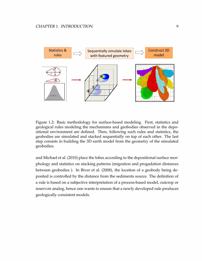
1.2 Basic methodology for surface-based modeling. First, statistics and
geological rules modeling the mechanisms and geobodies observed
in the depositional environment are defined. Then, following such
rules and statistics, the geobodies are simulated and stacked sequen-
tially on top of each other. The last step consists in building the 3D
earth model from the geometry of the simulated geobodies. . . . . . 9
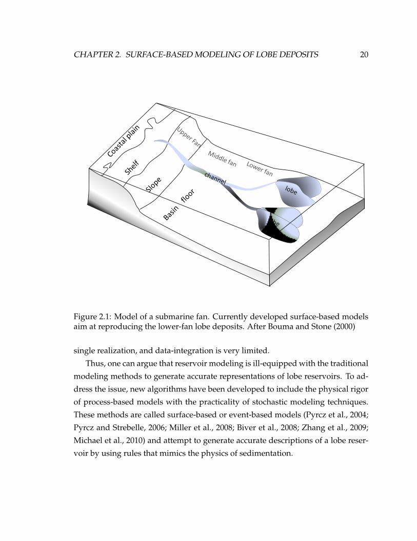
2.1 Model of a submarine fan. Currently developed surface-based mod-
els aim at reproducing the lower-fan lobe deposits. After Bouma
and Stone (2000) . . . . . . . . . . . . . . . . . . . . . . . . . . . . . . . 20
2.2 The fundamental building block of a turbidite lobe system is the
sand bed, which corresponds to a single flow event. A set of sand
beds forms a lobe-element. Lobe-elements form lobes, and lobes
form lobe-complexes. All the structures are embedded and present
similar elongated shapes. From Prelat (2009). . . . . . . . . . . . . . . 21
xi

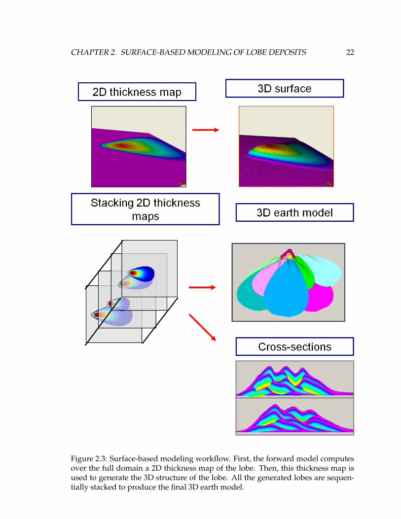
2.3 Surface-based modeling workflow. First, the forward model com-
putes over the full domain a 2D thickness map of the lobe. Then,
this thickness map is used to generate the 3D structure of the lobe.
All the generated lobes are sequentially stacked to produce the final
3D earth model. . . . . . . . . . . . . . . . . . . . . . . . . . . . . . . . 22
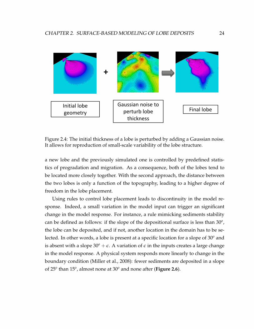
2.4 The initial thickness of a lobe is perturbed by adding a Gaussian
noise. It allows for reproduction of small-scale variability of the lobe
structure. . . . . . . . . . . . . . . . . . . . . . . . . . . . . . . . . . . . 24
2.5 Each of the two depositional models produces a different probabil-
ity map of lobe locations. Using the Tau model, it is possible to com-
bine these two probability maps into a single one (Journel, 2002).
The Tau value controls the relative importance of each model in the
final map. It therefore influences the stacking patterns of the lobes.
(CDF=cumulative distribution function) . . . . . . . . . . . . . . . . . 25
2.6 Due to the instability of sediments, no deposition occurs when the
depositional surface slope is more than 30o. Enforcing such behav-
ior using a rule (figure on the left) would mean that the lobe sedi-
mentation is not modified before the 30o threshold is reached. After
that, the lobe location is shifted to another location, creating discon-
tinuities in the model response. Similar discontinuities do not oc-
cur with process-based models because physical processes respond
smoothly to small changes in the environmental conditions (figure
on the right). . . . . . . . . . . . . . . . . . . . . . . . . . . . . . . . . . 26
xii

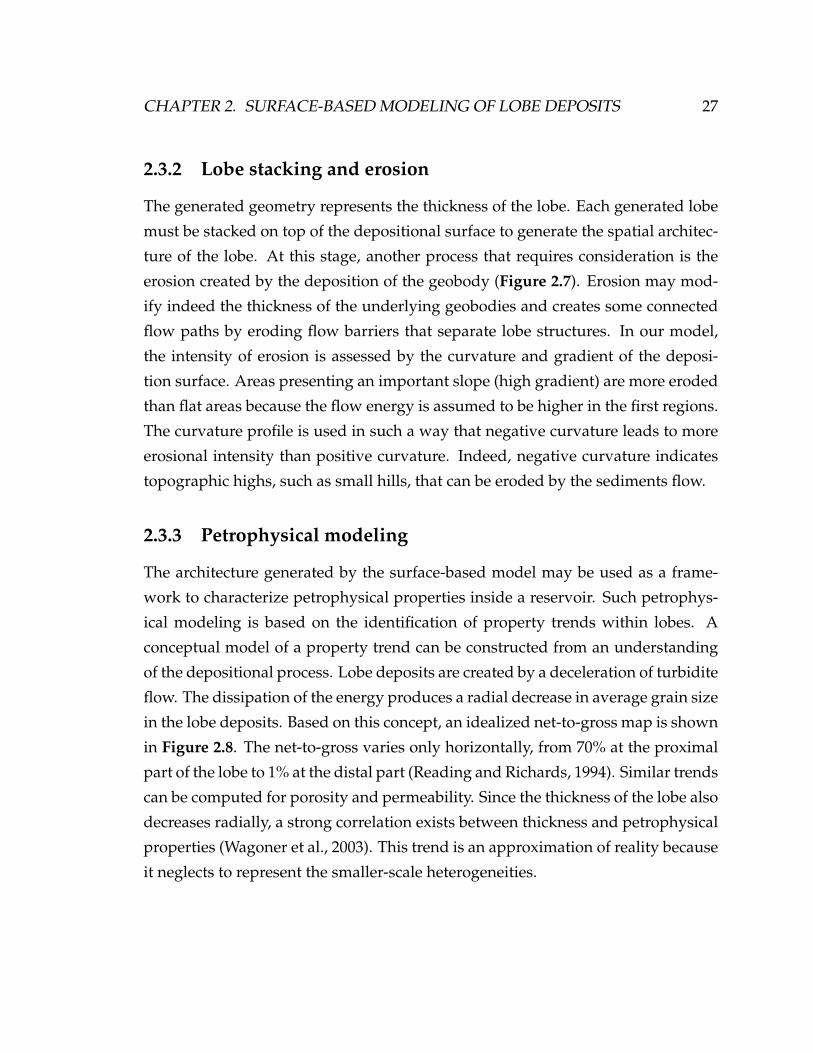
2.7 The erosion process associated with a lobe sedimentation is com-
puted in four steps. The first step consists of delimiting the re-
gion where the geobody is deposited. Then, based on the geological
model, the intensity of erosion is computed. An erosion surface is
then created by modifying the geometry of the underlying geobod-
ies. Lastly, the new lobe is deposited on top of this erosion surface.
In general, the erosion process is more pronounced near the source
of the lobe and where the topography has a positive curvature, a
high slope and a high elevation. . . . . . . . . . . . . . . . . . . . . . . 28
2.8 Net-to-gross trend within a lobe. . . . . . . . . . . . . . . . . . . . . . 29
2.9 Comparison of cross-sections of the process-based model (on the
left) and a surface-based model (on the right) for a small lobe sys-
tem. The top pictures represent the entire sedimentary structure.
The bottom one shows only the shale layers. We observe that surface-
based models can reproduce sedimentary structures that are realis-
tic when compared to process-based models, but at a fraction of the
CPU-costs. Courtesy from Li (Li et al., 2008) . . . . . . . . . . . . . . . 31
2.10 Summary of the rules and parameters needed to run a simulation
(see also Michael et al. (2010)). The parameters are highly uncertain
because they are difficult to infer. They are represented in the form
of probability distributions. To generate a realization, the parameter
values are drawn from these probability distributions. (CDF=cumulative
density function). . . . . . . . . . . . . . . . . . . . . . . . . . . . . . . 32
2.11 Gridding of a lobe. Stratigraphic grids can be built from the sur-
faces generated by the surface-based algorithm. This grid serves as
a support for properties characterization. . . . . . . . . . . . . . . . . 33
xiii
3.1 Surface-based models present two stochastic processes. The first
one is due to input parameter uncertainty. To run a simulation,
input values are randomly drawn from probability distributions.
Some of these parameters are then used to define a probability map
of lobe locations. This represents the spatial uncertainty; a set of in-
put parameters only narrows the possible locations of a lobe over
the domain, and the exact location is randomly selected from this
probability map. Both of those stochastic processes control the out-
put variability. . . . . . . . . . . . . . . . . . . . . . . . . . . . . . . . . 39
3.2 Workflow for sensitivity analysis. First, a distance matrix is com-
puted between the generated models. The models are then mapped
in the Euclidian space and from the Euclidian space to the feature
one. A clustering is achieved in the feature space, and based on how
parameters relate to the clusters, a sensitivity analysis is performed. . 43
3.3 Possible modifications of a simplex applied to a problem in two di-
mensions. . . . . . . . . . . . . . . . . . . . . . . . . . . . . . . . . . . 45
3.4 Traditionally, a Gaussian noise is generated by defining a variance,
covariance and seed. This seed controls the stochastic component
of the algorithm. In terms of optimization, generating a noise using
this approach is not convenient because a small perturbation of the
seed completely changes the noise structure, inducing discontinu-
ities in the objective function. Generating a Gaussian noise using the
gradual deformation method avoids this issue (Hu, 2000). Thanks
to this method, the stochastic process is controlled by a continuous
parameter and not a random seed; a small change in this parameter
generates a slight deformation of the noise, thus causing a smooth
variation in the objective function in terms of perturbing the Gaus-
sian noise. . . . . . . . . . . . . . . . . . . . . . . . . . . . . . . . . . . 47
xiv

3.5 Optimization workflow. The main inverse problem is solved se-
quentially. General parameters are first optimized; then, the opti-
mization focuses on the geometry and location of the first lobe. Each
step requires optimizing a relatively small number of parameters. . . 51
4.1 a) Bottom surface. b) Top surface. c) Sediment thickness. Sedimen-
tation occurs mainly around the sediment source, which is assumed
to be unique and located inside the red window. . . . . . . . . . . . . 56
4.2 1) Histogram representing the mismatch with data when the param-
eters uncertainty only is considered. The variance is 3.2. 2) His-
togram representing the mismatch with data when the spatial un-
certainty only is considered. The variance in mismatch is 0.83. . . . . 60
4.3 Pareto plot showing the importance of each parameter on the data-fit. 62
4.4 The lobe n is perturbed with two different noises. The first noise
creates a low topography on the right of the lobe. The following
lobe logically fills it (left pictures). The second noise creates a low
topography on the left of the lobe, generating sedimentation in this
location (right pictures). This example shows the importance of the
noise in the placement of the lobes . . . . . . . . . . . . . . . . . . . . 63
4.5 Result of the optimization method. The larger errors in terms of
misfit with data are located near the sources, where the erosion is
very pronounced. . . . . . . . . . . . . . . . . . . . . . . . . . . . . . . 66
4.6 Well log data recorded in the optimized model and data. . . . . . . . 67
4.7 Cross-section of the model at different steps of the optimization pro-
cess. Each lobe is represented by a different colored zone. . . . . . . . 68
4.8 Three matching models generated from different initial guesses. . . . 69
4.9 Performance results of the different optimization approaches. At
the top, the evaluation is based on the number of iterations. At the
bottom, the evaluation is based on the computational time (hours). . 72
5.1 Different scales of structures are present inside a lobe system (Prelat
et al., 2009). . . . . . . . . . . . . . . . . . . . . . . . . . . . . . . . . . . 76
xv

5.2 Hierarchical workflow for modeling lobe-elements within lobes. The
larger-scale elements, the lobes, are simulated first. Lobe-elements
are then embedded inside them using our conditioning methodology. 77
5.3 Top and bottom surfaces of the MS1 reservoir. . . . . . . . . . . . . . 79
5.4 MS1 wells data. Each well offers information on the lobes and lobe-
elements thickness, a lobe being composed of a set of lobe-elements.
. . . . . . . . . . . . . . . . . . . . . . . . . . . . . . . . . . . . . . . . 80
5.5 The input parameters are inferred from a physical-based model pre-
senting similar depositional settings. A process-based model con-
tains a continuous succession of sediments. Identifying sedimentary
objects from the model requires a subjective interpretation, which
leads to uncertain input parameters. . . . . . . . . . . . . . . . . . . . 83
5.6 1) Histogram representing the mismatch with data when only the
parameter uncertainty is considered. The variance is 3.7. 2) His-
togram representing the mismatch with data when only the spatial
uncertainty is considered. The variance in mismatch is 1.4. . . . . . . 84
5.7 Pareto plot showing the importance of each parameter on the data-fit. 85
5.8 In the first picture above, the reservoir top surface as defined in the
data. In the middle, the top surface of the reservoir as generated
by the surface-based model. At the bottom, the corresponding error
map is presented. . . . . . . . . . . . . . . . . . . . . . . . . . . . . . . 87
5.9 The internal layering of the reservoir at the lobe-element scale. . . . . 88
5.10 1) Histogram representing the mismatch with data when only the
parameter uncertainty is considered. The variance is 4.3. 2) His-
togram representing the mismatch with data when only the spatial
uncertainty is considered. The variance in mismatch is 1.9. . . . . . . 90
5.11 Pareto plot showing the importance of each parameter on the data-fit. 91
5.12 The internal layering of the reservoir at the lobe-element scale. . . . . 93
xvi

5.13 A) Top surface of the lobe simulated with the surface-based model.
B) Top surface of the stack of lobe-elements embedded in the lobe.
The match between the two structures is very strong. The higher
roughness of the surface B is caused by the stacking of distinct geo-
bodies. . . . . . . . . . . . . . . . . . . . . . . . . . . . . . . . . . . . . 94
5.14 A) Bottom and top surfaces of lobe B) Internal layering of lobe-
elements inside a lobe. . . . . . . . . . . . . . . . . . . . . . . . . . . . 95
6.1 The presented conditioning workflow consists of dividing the full
optimization problem into smaller ones that are easier to solve. Each
sequence is solved using a hybrid optimization. A population of in-
dividuals is first optimized with a genetic algorithm. The best so-
lution obtained from the genetic algorithm is then optimized with
Nelder-Mead. . . . . . . . . . . . . . . . . . . . . . . . . . . . . . . . . 99
6.2 Location of the Tanqua Fan Complex fan in South Africa . . . . . . . 100
6.3 Locations of the wells in the domain. Two flow events originat-
ing from the South-East and the South-West of the domain created
the observed structures. The sources of sediments are not exactly
known, but they are assumed to be located inside the two windows. 101
6.4 On the right, the histogram representing the mismatch with data
when only the parameters uncertainty is considered. The variance
is 2.5. On the left, the histogram representing the mismatch with
data when only the spatial uncertainty is considered. The variance
in mismatch is 2.6 . . . . . . . . . . . . . . . . . . . . . . . . . . . . . . 104
6.5 Pareto plot showing the importance of each parameter or combina-
tion of parameters on the data-fit. None of the parameters statis-
tically impact the model response (the level of significance is not
reached). One of the possible reasons is the spatial stochasticity that
can alter the sensitivity analysis results, making it difficult to iden-
tify the leading parameters. . . . . . . . . . . . . . . . . . . . . . . . . 105
xvii
6.6 Performance results of the different hybrid schemes. GA stands for
genetic algorithms and NM for Nelder-Mead. The specified per-
centage indicates the proportion of forward simulations (function
evaluations) allocated to GA and NM. . . . . . . . . . . . . . . . . . . 108
6.7 Model generated by the hybrid optimization approach. A) Initial
depositional surface. B) Top surface of the sediments package. C)
Lateral section of the model. D) Longitudinal section of the model. . 110
6.8 Sequence of deposition for the lobes for the model generated with
the hybrid optimization. . . . . . . . . . . . . . . . . . . . . . . . . . . 111
6.9 Model generated with the hybrid approach method and correspond-
ing match with the well data. . . . . . . . . . . . . . . . . . . . . . . . 112
6.10 Model generated with the Nelder-Mead method and corresponding
match with the well data. . . . . . . . . . . . . . . . . . . . . . . . . . 113
6.11 Left: Cross-plot between measured lobe thicknesses in the data and
the mismatches of the model after a hybrid optimization. Right:
Cross-plot between measured net-to-gross in the data and mismatches
of the model after a hybrid optimization. . . . . . . . . . . . . . . . . 114
6.12 To study the model predictions, a wells is removed from the data-
set. When models are conditioned to the remaining wells, the struc-
tures generated at the removed wells location are extracted and com-
pared to the real ones. This method allows therefore the predictive
accuracy of the surface-based models. . . . . . . . . . . . . . . . . . . 119
6.13 On top: cross-plot between computational time and data-fit accu-
racy. Bars represent the spread from worst to best data-fit given a
computational time. At bottom: cross-plot between computational
time and model predictions. Bars represent the spread from worst
to best prediction given a computational time. . . . . . . . . . . . . . 120
6.14 Example of two gaussian likelihood functions. A low variance means
that the rejection algorithm is very selective and accepts only mod-
els with small misfit. . . . . . . . . . . . . . . . . . . . . . . . . . . . . 121
xviii

6.15 Comparison between predictions generated with the optimization
method and a rejection sampling algorithm. For the optimization,
the predictions are calculated with increasing computational time
(hence increasing matching accuracy). For the rejection sampling,
the predictions are computed with increasing likelihood selectivity
(increasing matching accuracy as well). The location of the red bar is
chosen so that, at this location, the average data-fit of the population
generated by optimization and by sampling are similar. . . . . . . . 122
6.16 Comparison between lobes thicknesses generated by rejection sam-
pling and our optimization approach. . . . . . . . . . . . . . . . . . . 123
6.17 Cross-sections of our model: the bottom lobes tend to be thicker
than the top ones. This bias is introduced by our sequential opti-
mization. . . . . . . . . . . . . . . . . . . . . . . . . . . . . . . . . . . 124
xix

Acknowledgement
Pursuing a PhD is a long journey. It tests your endurance and tenacity as much as
your academic prowess. Yet, when it comes to the end, what remain in my mind
are pride and happiness. Such journey would not have been possible without the
help and support of many people. First of all, I would like to express my utmost
gratitude towards my advisor, Prof. Jef Caers for his guidance, encouragement,
critical feedback. During my four years in Stanford, I learned tremendously from
Jef, not only in research, but also in many others aspects that will be beneficial to
all my life, such as how to write in an efficient way, how to face technical difficul-
ties or how to communicate with people. All his inputs and advices are, and will
remain, invaluable to me. Thanks are also due to Hamdi Tchelepi, Louis Durlofsky,
Roalnd Horne and Gary Mavko for serving on my PhD committee . Two advisors
from my internships at Exxon also deserve special recognition for their support:
Tao Sun and Hongmei Li. Without their precious inputs, applying my PhD ideas
to real-world problem would have impossible. It was a delight to work with such
a smart and knowledgeable team. The next thanks go to my fellow Stanford col-
leagues and friends: Guillaume, Cedric, Matthieu, Sebastien, Bruno, Danny, Ce-
line, Mehrdad, Markus, Gregoire, Emmanuel and many others... Thanks to them,
my stay in Stanford was fun and entertaining, creating timeless memories. I also
would like to thank my family. They gave me their love and support through ev-
ery stage of my education and my life. I am forever grateful to them. Last, but
by no means least, I thank Lisa for her daily support and the happiness she has
brought to my life.
1
Chapter 1
Introduction
Oil exploration and production involves finding hydrocarbon deposits and devel-
oping them for commercial use. Various data acquisition techniques are employed
to understand the structures and properties of a reservoir. The generated data pro-
vide information at different scales. Log measurements record properties locally
around the well. Seismic surveys cover large volumes, but their accuracy is low
(meters vertically, tens of meters horizontally) compared to well-log data. There-
fore, geologic interpretations, based on available information and understanding
of sedimentary processes, are used to interpolate or extrapolate the measured data
in order to yield complete reservoir descriptions. This step is called reservoir mod-
eling. Given the different scales of geological structures existing in the reservoir
and the difference in data accuracy, the reservoir model is built hierarchically. First,
the architecture of elements interpreted at the seismic scale is included determin-
istically in the reservoir model. These structures can indeed be identified or inter-
preted from seismic data and well markers. The defined structures are in general
stratigraphic horizons and faults. A stratigraphic horizon corresponds to a change
in the nature of the deposited sediments (fluvial then deltaic sediments, for ex-
ample). Each specific sediment package, which is bounded by two stratigraphic
horizons, is called a layer. The sedimentary structures present inside a layer are
2

CHAPTER 1. INTRODUCTION 3
too small to be explicitly identified in the seismic data. Instead, their characteriza-
tion is achieved using stochastic modeling approaches. Developing and improv-
ing those stochastic modeling approaches have always been a focus of petroleum
studies because these subseismic scale elements may impose a significant control
on the reservoir flow response.
1.1 Property modeling
The spatial organization of sediments inside a layer is driven by deposition and
erosion processes. In such physical systems, self-organized structures emerge from
the interactions between fluid motion and geomorphological processes (Madej,
2001). For example, coarse sediments flowing with high energy from a source
to a flat land are not randomly deposited. First, the high energy flow generates
channels with a straight path. Then, due to the instability of the flow, perturba-
tions in the channels path are introduced, producing increasing channels curva-
tures. The coarse sediments are ultimately gathered in the form of typical curvi-
linear patterns (Hallet, 1990; Grant et al., 1990). Depending on the characteristics of
the depositional environment and the scale of the physical process, different self-
organized patterns emerge from the sediments transport: dunes from the wind,
delta from the decharge of a river in the ocean, etc.
A self-patterning phenomenon create a spatial continuity in the reservoir, mak-
ing prediction possible: when a well intersects a lobe structure, another well drilled
a couple a meters away will have a high probability of intersecting the lobe too.
Consequently, models of spatial continuity can be used to assess the properties val-
ues within the reservoir. The next section reviews the existing models and presents
their corresponding advantages and limitations (Figure 1.1).
1.1.1 Two-point geostatistics
With two-point geostatistics, the estimation of a value at an unsampled location is
performed by linear combination of the measured data. The weight assigned to
CHAPTER 1. INTRODUCTION 4
each data is based on the degree of correlation between the data and the unsam-
pled location. This degree of correlation is provided by the variogram (Goovaerts,
1997). Such model of spatial continuity, by only incorporating the correlation be-
tween two points in space at a time, fails to capture the geometrical complexity
of sediments structures. Curvilinear channels, for instance, cannot be reproduced.
The popularity of such methods is due to their computation and data-integration
efficiency.
1.1.2 Multiple-point geostatistics
Since the heterogeneities present inside a reservoir are too complex to be rep-
resented only by a two-point correlation model, multiple-point statistical (MPS)
techniques (Strebelle, 2002; Zhang et al., 2006; Arpart and Caers, 2007) have been
developed to provide a value at an unstamped location based on the configuration
of more than two points. This allows simulating complex, non-linear spatial rela-
tionships. Inferring directly the multiple-point statistics from the subsurface data
is impossible because data are too sparse. Instead, the statistics are inferred from
a training image, which is a representation of the assumed subsurface structures.
The training image can be built from physical-based models, geologists drawings,
pictures of on outcrop etc. Multiple-point geostatistics have been successfully ap-
plied to complex sedimentary environments, such as fluvial systems (Strebelle and
Zhang, 2004), turbidite reservoirs (Strebelle et al., 2003) and carbonate plateforms
(Levy et al., 2008). Like two-point statistics, MPS models are easily conditioned to
data, though simulations on large grids can be computationally intensive.
1.1.3 Object-based model
Object-based methods consist of placing stochastically pre-defined geobodies within
a domain until some constraints (such as net-to-gross ratios) are met (Shmaryan
and Deutsch, 1999; Deutsch and Wang, 1996). One advantage of the method is the
realism and accuracy of the generated objects. A channel can be defined by mul-
tiple parameters: width, length, amplitude, thickness, or presence of a sand bar;

CHAPTER 1. INTRODUCTION 5
a carbonate mound by its shape (conical or ring shape), size or facies distribution
and so on. The nature of the relationship between objects can also be specified
as a model input. Channels can be forced to be positioned close to each others (at-
traction) in order to reproduce the channels amalgamation observed in deep-water
systems. Although object-based simulation is fast, data conditioning is challeng-
ing. It often must proceed as a trial-and-error fashion, significantly increasing CPU
times . Consequently, a common application for object-based methods is to gen-
erate training images for multiple-point statistics; complex sedimentary structures
can be easily generated without any need for data conditioning.
1.1.4 Process-based model
The methods previously presented focus on analyzing and processing the geom-
etry of the sedimentary structures. Two-point geostatistics model heterogeneities
based on a variogram, which defines the correlation between a pair of points as a
function of their distance. Multiple-point statistics reproduce the geometric pat-
terns observed in a layer of sediments. Object-based methods generate sedimen-
tary structures from a template geometry.
However, the emergence of specific sedimentary structures is driven by com-
plex physical processes that occur both in space and in time. By neglecting the
temporal dimension, traditional modeling methods fail to reproduce the complex
interactions of topography, flow, deposition and erosion. Yet, representing these
interactions accurately is crucial to model realistically the reservoir heterogeneities
when (1) the reservoir structures and compartmentalization have been shaped by a
series (in time) of sedimentation and erosion events; and (2) few data are available
to help to delineate the reservoir heterogeneities and discontinuities.
This situation occurs commonly in deep offshore turbidite reservoirs develop-
ment. Turbidite reservoirs are indeed created by large and episodic sedimentary
events, and the key factors controlling the distribution of sand and shale are the
seafloor morphology and the supply of sediments (Bouma et al., 1985; Mutti and
Tinterri, 1991). Furthermore, available data are limited at any stage of development

CHAPTER 1. INTRODUCTION 6
due to the high cost of acquisition. Traditional modeling methods can capture
some of the heterogeneities. The shape of the channels or lobes can be reproduced
using multiple-point statistics or object-based models. However, such methods fail
to reproducing how a channel erodes the underlying sediments and modifies the
spatial continuity of existing flow barriers, or how this channel becomes eroded by
ulterior geobodies. Properly considering erosion and deposition patterns requires
a model that can reproduce a sequence of sedimentary events.
Process-based models (also called physical-based models), by reproducing the
reservoir genesis, can provide a highly realistic representation of the subsurface
structures. The models simulate over-time the physical processes that formed the
sediments architecture. However, such simulation may require days, sometimes
weeks, of computation time because it involves solving complex differential equa-
tions: conservation of flow momentum, conservation of fluid, conservation of sed-
iments and balance of turbulent kinetic energy (Miller et al., 2008). Hence, the use
of these models in reservoir characterization is limited by the associated computa-
tion cost. The problem is especially acute for data integration since iterations on
the model require a tremendous amount of CPU power (Miller et al., 2008).

CHAPTER 1. INTRODUCTION 7
1.2 Surface-based modeling
Although building reservoir models with respect to data using process-based mod-
els is almost impossible, unconditional realizations are highly informative on the
sediments architecture and their spatial continuity (Miller et al., 2008; Michael
et al., 2010). Based on such information, a new family of stochastic models, termed
surface-based models or event-based models, has recently been developed (Fig-
ure 1.2). They do not fully reproduce the sedimentary processes but mimic them
with considerable realism using geological rules, producing key geological fea-
tures at a fraction of the process-based models CPU (Pyrcz et al., 2004; Pyrcz and
Strebelle, 2006; Miller et al., 2008; Biver et al., 2008; Zhang et al., 2009; Michael
et al., 2010). Such surface-based models have been primarily developed for tur-
bidite lobe systems, but the approach is general, and can be applied to other envi-
ronments of deposition as well as geometries other than lobes.
The existing models are based on a similar geobody stacking workflow. First
the model starts by specifying the geometry of the geobody being deposited. Then,
its location of sedimentation is selected according to certain geological rules. The
rules aim at mimicking the sedimentary processes that occur in the environment of
deposition. The new geobody is stacked on top of the current depositional surface,
which can be locally eroded in the process. The geobody top surface is merged
with this topography. This new surface then becomes the current depositional sur-
face. The stacking is repeated until a stopping criterion is reached. Such models
are stochastic because the parameters values used to perform a forward simula-
tion (size of the geobodies, location of the source, etc.) are uncertain and therefore
randomly drawn from probability distributions.
All existing surface-based models use a similar geobody-stacking workflow.
They differ, however, by the geological rules they employ. Pyrcz et al. (2004), Pyrcz
and Strebelle (2006) and Zhang et al. (2009) apply rules that are based on the eleva-
tion of the depositional surface; geobodies are more likely to fill topographic lows
and bypass high elevation areas. The methods presented by Miller et al. (2008)

CHAPTER 1. INTRODUCTION 8
Process based
Two points geostat.
Multi points geostat
Object based
Surface based
Figure 1.1: Different techniques exist to model subsurface structures. Two-pointgeostatistics, multiple-point geostatistics and object-based approaches focus onreproducing heterogeneities by matching observed patterns (pure geometric ap-proach), whereas surface-based and process-based models account for the pro-cesses that created the observed patterns. Therefore, those two methods producetherefore more realistic models. Their conditioning capabilities limit however theiruse.
CHAPTER 1. INTRODUCTION 9
Statistics & rules
Statistics & rules
Sequentially simulate lobes Sequentially simulate lobes with featured geometry
Construct 3D Construct 3D model
Figure 1.2: Basic methodology for surface-based modeling. First, statistics andgeological rules modeling the mechanisms and geobodies observed in the depo-sitional environment are defined. Then, following such rules and statistics, thegeobodies are simulated and stacked sequentially on top of each other. The laststep consists in building the 3D earth model from the geometry of the simulatedgeobodies.
and Michael et al. (2010) place the lobes according to the depositional surface mor-
phology and statistics on stacking patterns (migration and progadation distances
between geobodies ). In Biver et al. (2008), the location of a geobody being de-
posited is controlled by the distance from the sediments source. The definition of
a rule is based on a subjective interpretation of a process-based model, outcrop or
reservoir analog, hence one wants to ensure that a newly developed rule produces
geologically consistent models.
CHAPTER 1. INTRODUCTION 10
1.3 Challenges of conditioning surface-based models
to data
The end goal of reservoir modeling is to predict the flow performance of a field
or to select drilling locations that may improve hydrocarbon recovery. However,
an exhaustive sampling of the reservoir is impossible, and the true structure of the
reservoir remains unknown. Yet, a prior geological knowledge exists: nature of
the sediments (channels, lobes), processes of sedimentation (fluvial or deep water
systems) , etc. This knowledge can be interpreted, for instance, from the regional
geological setting of the reservoir. Some data also illumanate the reservoir struc-
ture: well-log measurements, seismic survey and production history. In order to
model a reservoir accurately, one needs to take into account both the prior geolog-
ical knowledge and the data. In the context of surface-based modeling, this means
generating a series of geobodies that fit the available data.
Surface-based models are forward-models in the sense that they predict the
nature of deposits given a set of initial parameters. It is not known a priori what
the deposits will look like and a matching model cannot be directly derived from
the data. Surface-based models are therefore difficult to directly constrain to data,
as many geostatistical methods do by construction. Since the input parameters
are uncertain, a possible solution for conditioning is to use an iterative approach,
where the output model is compared with the data and the input parameters by
trial-and-error methods updated in accordance to the mismatch. However, solving
this inverse problem is challenging. First, the inverse problem is commonly ill-
posed; the solution may not exist and, if a solution does exist, it may be non-unique
and not continuously dependent on the data. Secondly, the number of parameters
to perturbed is very large. Thirdly, the model may respond discontinuously to
changes in certain input parameters. In addition, the diversity in data available in
reservoir modeling (geological, geophysical and flow data) makes the conditioning
process even more complex.
Conditioning of surface-based modeling has not been extensively investigated
since most existing research has focused on developing the forward model itself.

CHAPTER 1. INTRODUCTION 11
The existing approaches are limited to well-data integration. The first approach,
developed by Pyrcz et al. (2004), is based on a local adjustment of the lobe sur-
face to fit the neighboring well data. When the surface geometry contradicts data
outside a tolerance, the geometry is rejected. The main limitation is the simula-
tion time associated with the rejection method. The second approach presented by
Zhang et al. (2009) is based on direct interpolation between logs. It necessitates a
large amount of wells, which is unrealistic in deep offshore development. The last
method, developed by Michael et al. (2010), achieves a match with well-data con-
ditioning using well correlation. Each of the depositional units must be identified
in well data and ordered according to the different depositional periods. However,
interpreting wells in such a detailed fashion is time-consuming and subject to un-
certainty. In addition, the interpretation correlation needs to be consistent with the
forward stratigraphic model.
Integration of data through inverse modeling has been investigated in quantita-
tive dynamic stratigraphy (Lessenger and Cross, 1996; Cross and Lessenger, 1999;
Charvin et al., 2009). Similarly to surface-based techniques, quantitative strati-
graphic methods predict geological structures by reproducing sedimentation pro-
cesses. Their main difference are found on the scale of interest (reservoir versus
basin), and the purpose of the study (assessing uncertainty for reservoir develop-
ment versus extracting stratigraphic parameters from data). The inverse methods
developed in quantitative dynamic stratigraphy are extremely costly to carry out
and mainly applied to 2D synthetic data (Lessenger and Cross, 1996; Charvin et al.,
2009). Applying them to real-world 3D problem would be extremely challenging
and too CPU-demanding. Alternatively to traditional inverse modeling, optimiza-
tion of the input parameters can provide an effective way to solve the conditioning
problem. However, the possibly large number of parameters to optimize makes
this approach problematic as well, especially since the model response may be dis-
continuous and efficient gradient-based techniques cannot be employed.

CHAPTER 1. INTRODUCTION 12
1.4 Proposed approach
In this context, we propose a new optimization methodology. The key idea behind
the method is to decrease the dimensionality of the optimization problem being
solved. Three complementary approaches are developed for this purpose:
1. Identification of the leading uncertainty. Surface-based models can account for
two types of uncertainties. The first uncertainty is on the input parameters,
such as geobodies sizes, locations of the sediments source or average inten-
sity of erosion, etc. The input parameters inference requires a subjective inter-
pretation of reservoir data, physical-based models or outcrops. The obtained
values are therefore subject to uncertainty and must be described with prob-
ability distributions.
The second uncertainty is the geobodies locations. For a given set of input
parameter values, the area where a geobody can be deposited is reduced to
a subpart of the domain but not to a unique location. In other words, a lobe
can have different locations for a specific set of input parameter values. The
uncertainty about the geobody location is called spatial uncertainty.
By performing two series of runs - one with only the input parameters uncer-
tainty considered, and the other with only the spatial uncertainty accounted
for - it is possible to determine which of the two uncertainties impact the
model output. Once the dominant uncertainty has been identified, only the
associated parameters require to be optimized, thus decreasing the dimen-
sionality of the conditioning problem.
2. Sensitivity analysis on the input parameters. A sensitivity analysis of the in-
put parameters can be performed to identify those that make the greatest
impact. The optimization can then focus only on a subset of parameters. Per-
forming a sensitivity analysis in the context of a high spatial uncertainty is
challenging because the spatial stochasticity alters the relationship input pa-
rameters/model outputs, making the sensitivity analysis results difficult to
analyze.

CHAPTER 1. INTRODUCTION 13
3. Re-formulation of the full optimization problem. Even when the two previous
steps are successful in simplifying the model, a significant number of param-
eters may remain. The parameters have to be optimized using derivative-
free algorithms since the model does not respond continuously to parame-
ters variations. The problem with derivative-free methods is their slowness
of convergence when a large numbermust be optimized. To circumvent this
issue, a divide-and-conquer approach is developed to solve sequentially the
optimization problem.
1.5 Dissertation outline
This conditioning methodology is general in the sense that it can be used with
any type of data and environments of deposition. We choose to focus our work
on turbidite lobe deposits and static data. As part of the validation and quality
control of the developed approach, the conditioning method is tested against three
real datasets composed of wells measurements and thickness maps. The forward
model used in this work was developed by Michael et al. (2010) and Leiva (2009).
The dissertation consists of seven chapters.
Chapter 2: Surface-based modeling . In the first part, a review of lobe deposits and
their associated modeling challenges is provided. We will also explain why tradi-
tional geostatistics methods present severe limitations for lobes modeling. The last
part describes the surface-based algorithm used to reproduce lobe deposits.
Chapter 3: Approach to data conditioning. This chapter provides a general opti-
mization framework used to fit surface-based models to data. The first part intro-
duces the possible methods of data integration for surface-based modeling. The
advantages of optimization for data conditioning are discussed. Finally, a condi-
tioning framework tailored for surface-based models is proposed.

CHAPTER 1. INTRODUCTION 14
Chapter 4: Application to the East-Breaks data set. The chapter presents an ap-
plication of the conditioning methodology to the East-Breaks data, a real data set
composed of three wells and a thickness map. The case study aims to demonstrate
the applicability and efficiency of the method.
Chapter 5: Hierarchical modeling workflow. In this chapter, the conditioning ap-
proach is applied in a specific way to generate multi-scale lobe structures. In-
deed, lobes do not form homogeneous sand bodies, and they are composed of
sub-elements, called lobe-elements. The lobe-elements are important to consider
because they may impact the flow inside a reservoir. To model such multi-scale
structures, we propose integrating our conditioning methodology with a hierar-
chical modeling workflow. The method is applied to a real dataset containing a
thickness map and wells. The wells in the data-set inform about both lobes and
lobe-elements thicknesses.
Chapter 6: Application to the Karoo dataset. The first part of the chapter presents
a challenging example in which the uncertainty and sensitivity analysis do not
lead to a simplification of the model. In order to handle the large number of pa-
rameters, a hybridization optimization algorithm is presented. The algorithm is
tested on a real data-set originating from the Karoo Basin. The second part of the
chapter highlights the drawbacks of optimization in term of uncertainty modeling.
Chapter 7: Conclusion and future work. The chapter discusses the contributions
and limitations of the presented work. Suggestions for future research investiga-
tions are also presented. They are divided in three parts. The first part provides
insights on how to enhance the surface-based model. The second part proposes
some ideas for improving the data-conditioning workflow. The last part exposes
the research needs required to develop a robust history-matching workflow.

Chapter 2
Surface-based modeling of lobe
deposits
2.1 Introduction
Chapter 2 provides an overview of surface-based modeling applied to turbidite
lobe systems. The first part of the chapter presents the characteristics and modeling
challenges of lobe deposits. Then, the second section describes the surface-based
algorithm used in this work to model the lobe deposits.
2.2 Geological background and modeling challenges
2.2.1 Turbidite systems
Turbidite systems are deposited over hundreds of thousands of years by series of
submarine gravity flows, which transport almost instantaneously sediments from
a shelf down a slope and onto a basin floor (Mutti and Normak, 1987). A turbidite
system is commonly divided into three parts called the upper, middle and lower
fans (Figure 2.1 Bouma et al. (1985)). The upper fan presents major channel fea-
tures and submarine canyons. The channels serve as conduits to transport the sed-
iments from the continental shelf to the basin floor. They are the last features to be
15
CHAPTER 2. SURFACE-BASED MODELING OF LOBE DEPOSITS 16
filled since all the sediments tend to be deposited further away in the basin. At the
base of the slope, which corresponds to the transition between the upper and mid-
dle fan, the flattening of the seafloor forces the gravity flow to start deposition in
this area. The type of deposition in the middle fan area consists of well-developed
channels filled with coarse grain sediments. However, a major part of the sedi-
ments bypasses the middle fan and ends up as lobes, corresponding to the lower
fan area.
The major sedimentary structures forming turbidite reservoirs are channels and
lobes (Mutti and Tinterri, 1991; Chapin et al., 1994). Both structures present very
different characteristics: their geometry, the processes of sedimentation, the corre-
sponding petrophysical properties. Surface-based models are general in fashion
and can be used with both families of objects. However, for illustrative purpose,
our work focuses on lobe deposits only.
2.2.2 Characteristics of lobe deposits
Lobes are created when the channels become too shallow and narrow to contain
the sediments. The sediments overflow from the channel and fan out, forming an
elongated sheet of sand. As different studies have shown, lobe deposits are not
an homogenous body of sand (Charvin et al., 1995; Garland et al., 1999) and a hi-
erarchy scheme can be developed to identify the different architecture elements
that build a lobe (Figure 2.2 Prelat et al. (2009)). The fundamental building block
is the sand bed, which represents a single depositional event. Their thickness is
in general less than 3 meters and their length a couple of hundred meters. When
stacked, beds form a lobe-element. Their lengths are around 4-5 km, with a width
of 2-3 km. Lobe-elements are usually less than 5 meters thick and do not contain
any fine grain units. However, they are separated from one another by fine grain
units (less than 5 cm thick) that can be eroded due to the amalgamation between
the lobe-elements. One or more lobe-elements stack to form a lobe. Lobes are typ-
ically 4 to 10 meters thick and with 3 to 10 lobe-elements (25 km x 15 km). They
are bounded by fine grain units, 0.2 to 2 meters thick units, which can be eroded

CHAPTER 2. SURFACE-BASED MODELING OF LOBE DEPOSITS 17
when new lobes are deposited. Lastly, lobes stack in lobe complexes (40 km x 30
km x 50m), which are bounded by thick fine grain units (2-20m). The shapes of all
these embedded structures are alike because they are created by a similar depo-
sitional flow type. Wagoner et al. (2003) proposed that the dominant mechanism
controlling the geometry of the deposits (lobe complex, lobe, lobe-element and
sand bed) is the deceleration associated with the transition from confined flow (in-
side a channel) to expanding flows (basin floor). The resulting structures present
a shape of an elongated leaf, with the thickness and grain size decreasing toward
the extremity of the deposits (Figure 2.8). The sedimentation of lobe-related de-
posits is controlled by the morphology of the depositional surface. Early lobes fill
topographic lows and create locally topographic highs. The subsequent lobes are
deposited in lows next to the previously deposited lobes, causing compensating
stacking patterns (Groenenberg et al., 2010).
Turbidite lobes form high-quality reservoirs. They present large areal extent
and lateral continuity (McLean, 1981). Porosity in lobes ranges from 20 to 35%,
and permeability from 100 to 2000 md. The average net-to-gross varies from 40%
to 60% (Fugitt et al., 2000; Saller et al., 2008). Turbidite fields with hydrocarbon
accumulations in lobes are ubiquitous: Balder in the North Sea (Bergslien, 2002),
Bullwinkle (Holman and Robertson, 1994), Lobster (Edman and Burk, 1998), Diana
(Sullivan et al., 2000), and Auger (McGee et al., 1994) in the Gulf of Mexico, or
Marlim offshore Brazil (Santos et al., 2000), etc. Lobe systems constitute therefore
major hydrocarbon reserves throughout the world.
In terms of reservoir characterization, modeling the lobes geometries as realisti-
cally as possible is critical because by being draped in shales, the lobes geometries
control the fluid flow through the reservoir (Fugitt et al., 2000; Li et al., 2008). De-
pending on the final extension of the shales layer, individual lobes can even act
as separate flow units. Shales occurring at smaller scales, especially at the lobe-
elements level, may impact the flow as well. In such cases, modeling them may be
desirable (Charvin et al., 1995). One factor controlling shale continuity is erosion
originating from the deposition of overlaying lobes.

CHAPTER 2. SURFACE-BASED MODELING OF LOBE DEPOSITS 18
2.2.3 Limitations of existing modeling approaches
A problem inherent to deepwater reservoir modeling is the scarcity of the data.
Only sparse wells and a seismic survey are usually available.
In general, the internal architecture of a deep-water lobe reservoir cannot be re-
solved using 3D seismic data because of limitations in seismic accuracy. Saller et al.
(2008) provides an example of a high-frequency (50Hz) seismic survey performed
on a shallow buried lobe reservoir. At 50Hz, the accuracy of the seismic image al-
lows for identification of the lobes inside the reservoir. When the seismic data are
filtered to remove the high frequency components, decreasing consequently the
image frequency content (i-e decreasing the resolution) to 40Hz, the lack of res-
olution prevents the geophysicists from distinguishing between the lobes clearly.
Most of the seismic data at exploration depth have frequency content of 30Hz-
40Hz at best (Steffens et al., 2006). Hence, deterministically modeling lobes from
seismic data is, in most cases, impossible. Notwithstanding, seismic data may in-
form the overall shape and thickness of the reservoir.
Wells are too sparse to inform precisely the reservoir internal architecture, espe-
cially during initial field development. Consequently, delineating lobes geometry
from the data is most of the time impossible and a model that can produce realistic
lobe geometry without relying on data is required. This disqualifies two-points
geostatistics since they can only produce Gaussian-like fields.
The use of multiple-point statistics would also present some limitations. In
multiple-point statistics, a requirement on the training image is the number of
pattern replicates; the training image should present enough pattern variability
in order to generate realistic structures. Lobe systems exhibit non-stationarity:
the system diverges from proximal to distal, and the lobes can present prograd-
ing stacking patterns. Accounting for non-stationarity in the training image is not
straightforward because it requires subdividing the image into smaller stationary
ones (Boucher, 2009; Honarkhah, 2011). The smaller images must be large enough
to contain sufficient patterns repetitions. This requires the initial training image to
be extremely large. Secondly, a particularity of lobe systems is that they contain

CHAPTER 2. SURFACE-BASED MODELING OF LOBE DEPOSITS 19
large objects, the lobes, but these are few in number (Prelat et al., 2009). It means
that a training image reproducing a lobe system may not contain enough patterns
replicates for efficient use. In addition, multiple-point statistics are not as efficient
in 3D as in 2D. Working with 3D templates is CPU-costly and the template size
is limited. Smaller templates yield realizations that do not reproduce accurately
the sedimentary objects observed in the training images. In our case, it means that
the shape of the lobes will not be reproduced, or that the spatial continuity of the
shales will be altered. Lastly, the lobe facies is simulated as a whole and there is no
knowledge of the individual objects. Identifying single lobes from multiple-point
statistics realizations may be difficult due to lobes crosscutting each other. This is
important since some of the objects may behave as separate flow units. One poten-
tial solution is coding the different lobes with different indicators such that distinct
objects and their boundaries can be identified. However, this requires extremely
large training images for patterns with similar indicators to be repeated frequently
enough.
A possible solution for modeling lobes is to use object-based methods because
they allow for the accurate characterization of large-scale objects. Object-based
models have been applied successfully to capture complex non-linear connectiv-
ities in channelized reservoirs (Deutsch and Wang, 1996). However, data condi-
tioning is extremely difficult. It is usually done by an inefficient trial-and-error
approach. Newer optimization-based approaches (Shmaryan and Deutsch, 1999)
are not yet able to achieve a match in a reasonable number of iterations. A sec-
ond issue relies on the object placement strategy. Lobes deposition is driven by
the morphology of the depositional surface, hence the previously deposited sedi-
ments. Object-based methods randomly place the object in a domain. They do not
track the evolution of the depositional surface after a sedimentary event. Thus, the
method cannot reproduce accurately the lobes stacking patterns.
Unlike multiple-point and object-based techniques, process-based methods can
generate geologically consistent lobe reservoirs by simulating the fundamental
physical processes of sedimentation. However, severe limitations exist due to the
associated computation costs. Days, sometimes weeks, are needed to perform a
CHAPTER 2. SURFACE-BASED MODELING OF LOBE DEPOSITS 20
Figure 2.1: Model of a submarine fan. Currently developed surface-based modelsaim at reproducing the lower-fan lobe deposits. After Bouma and Stone (2000)
single realization, and data-integration is very limited.
Thus, one can argue that reservoir modeling is ill-equipped with the traditional
modeling methods to generate accurate representations of lobe reservoirs. To ad-
dress the issue, new algorithms have been developed to include the physical rigor
of process-based models with the practicality of stochastic modeling techniques.
These methods are called surface-based or event-based models (Pyrcz et al., 2004;
Pyrcz and Strebelle, 2006; Miller et al., 2008; Biver et al., 2008; Zhang et al., 2009;
Michael et al., 2010) and attempt to generate accurate descriptions of a lobe reser-
voir by using rules that mimics the physics of sedimentation.

CHAPTER 2. SURFACE-BASED MODELING OF LOBE DEPOSITS 21
Figure 2.2: The fundamental building block of a turbidite lobe system is the sandbed, which corresponds to a single flow event. A set of sand beds forms a lobe-element. Lobe-elements form lobes, and lobes form lobe-complexes. All the struc-tures are embedded and present similar elongated shapes. From Prelat (2009).
2.3 Concepts of Surface-based models
From the previous chapter, we have seen that (a), lobes have a typical elongated
shape, (b) the location of deposition is partially controlled by the morphology of
the depositional surface, and (c) the sedimentation of a lobe, by modifying the mor-
phology of the depositional surface, influences the sedimentation of the following
lobes.
The algorithm used in the following work, based on Michael’s research (Leiva,
2009; Michael et al., 2010), mimics these deposition characteristics. For a given
topography, the model starts by generating a new lobe based on a geometry tem-
plate with lobe length, width and height drawn for probability distributions (a).
The lobe location is selected according to deposition rules that process the mor-
phology of the depositional surface (b). The new lobe is stacked on top of the
current topography. The lobe’s top surface is merged with this topography. This
new surface then becomes the current topography (c). The process is repeated until
the reservoir is filled (Figure 2.3). Note that, in surface-based modeling, the term
event refers to the deposition of a geobody (a lobe here) and should not be con-
fused with a turbidity event, which corresponds to a single gravity flow. Several
gravity flows are required to produce a single lobe.
CHAPTER 2. SURFACE-BASED MODELING OF LOBE DEPOSITS 22
Figure 2.3: Surface-based modeling workflow. First, the forward model computesover the full domain a 2D thickness map of the lobe. Then, this thickness map isused to generate the 3D structure of the lobe. All the generated lobes are sequen-tially stacked to produce the final 3D earth model.

CHAPTER 2. SURFACE-BASED MODELING OF LOBE DEPOSITS 23
2.3.1 Lobe generation
Geometry definition
In a surface-based approach, the goal is not to reproduce the objects with high de-
tails but rather to replicate their general structures. Therefore, lobes are simulated
using a predefined geometry template. The shape of the lobes is described by the
following equation:
R = Lcos(2θ), x = Rcos(θ), y = Wsin(θ) (2.1)
where L is the length of the lobe, W the width, and θ ∈ [0− 2π]. The actual
size of a lobe is drawn from probability distributions. Based on this shape, a 2D
thickness property is defined such that the center of the lobe reaches a maximum
thickness, creating a 3D structure. This parameterization reproduces the overall
shape of the lobe. This idealized thickness map is then stochastically perturbed by
adding a Gaussian-correlated noise generated with a Sequential Gaussian Simula-
tion, (SGS, Goovaerts (1997)). The noise models the smaller scale variability of the
lobe’s structure (Figure 2.4).
Lobe placement
The location of a lobe is randomly drawn from a probability map (Figure 2.5). Two
sets of rules are used to compute the map. Both rules aim at reproducing the ten-
dency of geobodies to fill topographic lows. The first approach computes proba-
bilities based on topographic elevation and distance between lobes. Such rules are
obtained from an existing process-based model representing a typical lobe system
(Michael et al., 2010). The second approach is only based on topographic features.
Both approaches produce a different probability map. These two maps are then
combined into a single one, using the Tau model (Journel, 2002). The variation
between 0 and 1 of the tau value emphasizes more or less one of the probabilities,
hence one of the depositional rules. With the first approach, the distance between
CHAPTER 2. SURFACE-BASED MODELING OF LOBE DEPOSITS 24
+
Initial lobe geometry
Gaussian noise to perturb lobe
thickness
Final lobe
Figure 2.4: The initial thickness of a lobe is perturbed by adding a Gaussian noise.It allows for reproduction of small-scale variability of the lobe structure.
a new lobe and the previously simulated one is controlled by predefined statis-
tics of progradation and migration. As a consequence, both of the lobes tend to
be located more closely together. With the second approach, the distance between
the two lobes is only a function of the topography, leading to a higher degree of
freedom in the lobe placement.
Using rules to control lobe placement leads to discontinuity in the model re-
sponse. Indeed, a small variation in the model input can trigger an significant
change in the model response. For instance, a rule mimicking sediments stability
can be defined as follows: if the slope of the depositional surface is less than 30o,
the lobe can be deposited, and if not, another location in the domain has to be se-
lected. In other words, a lobe is present at a specific location for a slope of 30o and
is absent with a slope 30o + ε. A variation of ε in the inputs creates a large change
in the model response. A physical system responds more linearly to change in the
boundary condition (Miller et al., 2008): fewer sediments are deposited in a slope
of 25o than 15o, almost none at 30o and none after (Figure 2.6).

CHAPTER 2. SURFACE-BASED MODELING OF LOBE DEPOSITS 25
Tau = 0
Tau = 1
Topographic approach- Curvature- Gradient- Elevation
Tau = 1/3
Tau = 2/3
Statistics approach- Migration cdf- Progradation cdf- Elevation
Probability map Example of lobe placement
20 40 60 80 100
10
20
30
40
50
60
70
80
90
100 0
0.5
1
1.5
2
2.5
3
3.5
x 10-3
Figure 2.5: Each of the two depositional models produces a different probabilitymap of lobe locations. Using the Tau model, it is possible to combine these twoprobability maps into a single one (Journel, 2002). The Tau value controls the rela-tive importance of each model in the final map. It therefore influences the stackingpatterns of the lobes. (CDF=cumulative distribution function)
CHAPTER 2. SURFACE-BASED MODELING OF LOBE DEPOSITS 26
Physic-based modelsSurface-based models
α = 0⁰
α = 15⁰
α = 30⁰
α = 30⁰+ε
α = 0⁰
α = 15⁰
α = 30⁰
α = 30⁰+ε
Lobe Lobe
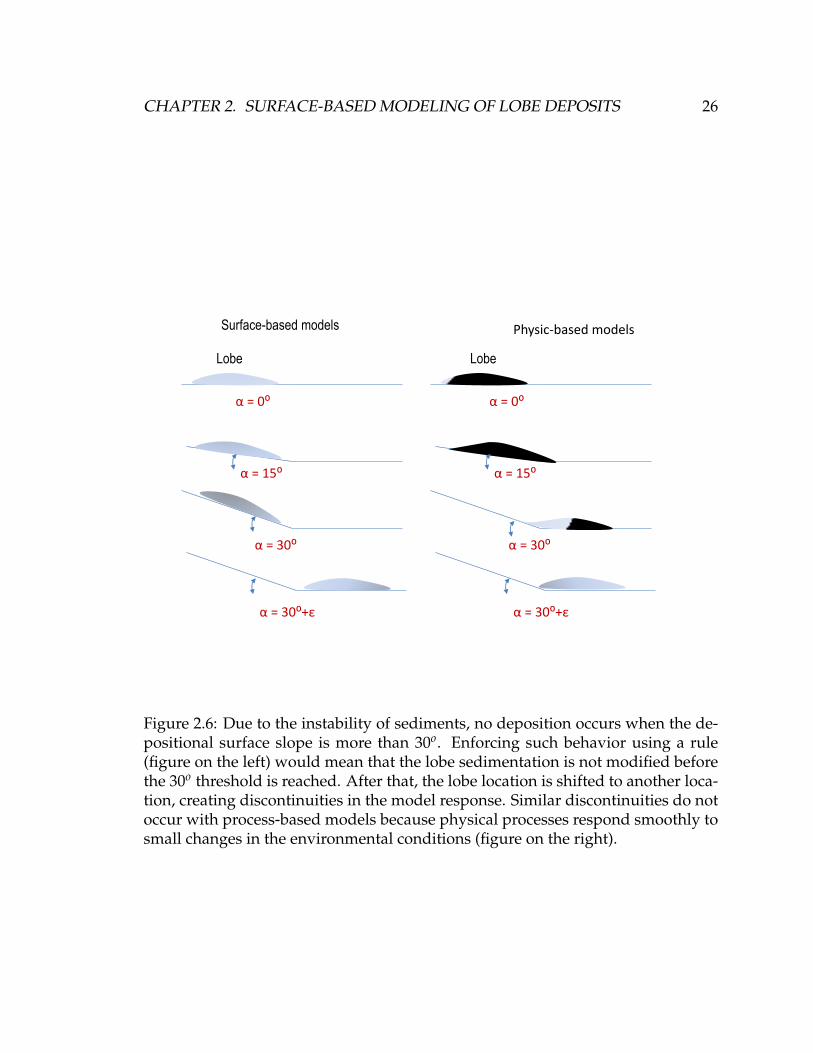
Figure 2.6: Due to the instability of sediments, no deposition occurs when the de-positional surface slope is more than 30o. Enforcing such behavior using a rule(figure on the left) would mean that the lobe sedimentation is not modified beforethe 30o threshold is reached. After that, the lobe location is shifted to another loca-tion, creating discontinuities in the model response. Similar discontinuities do notoccur with process-based models because physical processes respond smoothly tosmall changes in the environmental conditions (figure on the right).
CHAPTER 2. SURFACE-BASED MODELING OF LOBE DEPOSITS 27
2.3.2 Lobe stacking and erosion
The generated geometry represents the thickness of the lobe. Each generated lobe
must be stacked on top of the depositional surface to generate the spatial architec-
ture of the lobe. At this stage, another process that requires consideration is the
erosion created by the deposition of the geobody (Figure 2.7). Erosion may mod-
ify indeed the thickness of the underlying geobodies and creates some connected
flow paths by eroding flow barriers that separate lobe structures. In our model,
the intensity of erosion is assessed by the curvature and gradient of the deposi-
tion surface. Areas presenting an important slope (high gradient) are more eroded
than flat areas because the flow energy is assumed to be higher in the first regions.
The curvature profile is used in such a way that negative curvature leads to more
erosional intensity than positive curvature. Indeed, negative curvature indicates
topographic highs, such as small hills, that can be eroded by the sediments flow.
2.3.3 Petrophysical modeling
The architecture generated by the surface-based model may be used as a frame-
work to characterize petrophysical properties inside a reservoir. Such petrophys-
ical modeling is based on the identification of property trends within lobes. A
conceptual model of a property trend can be constructed from an understanding
of the depositional process. Lobe deposits are created by a deceleration of turbidite
flow. The dissipation of the energy produces a radial decrease in average grain size
in the lobe deposits. Based on this concept, an idealized net-to-gross map is shown
in Figure 2.8. The net-to-gross varies only horizontally, from 70% at the proximal
part of the lobe to 1% at the distal part (Reading and Richards, 1994). Similar trends
can be computed for porosity and permeability. Since the thickness of the lobe also
decreases radially, a strong correlation exists between thickness and petrophysical
properties (Wagoner et al., 2003). This trend is an approximation of reality because
it neglects to represent the smaller-scale heterogeneities.
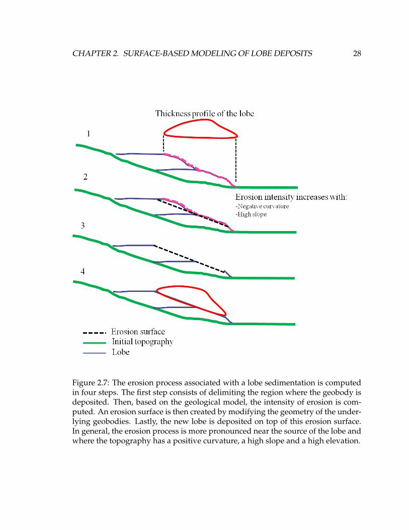
CHAPTER 2. SURFACE-BASED MODELING OF LOBE DEPOSITS 28
Figure 2.7: The erosion process associated with a lobe sedimentation is computedin four steps. The first step consists of delimiting the region where the geobody isdeposited. Then, based on the geological model, the intensity of erosion is com-puted. An erosion surface is then created by modifying the geometry of the under-lying geobodies. Lastly, the new lobe is deposited on top of this erosion surface.In general, the erosion process is more pronounced near the source of the lobe andwhere the topography has a positive curvature, a high slope and a high elevation.
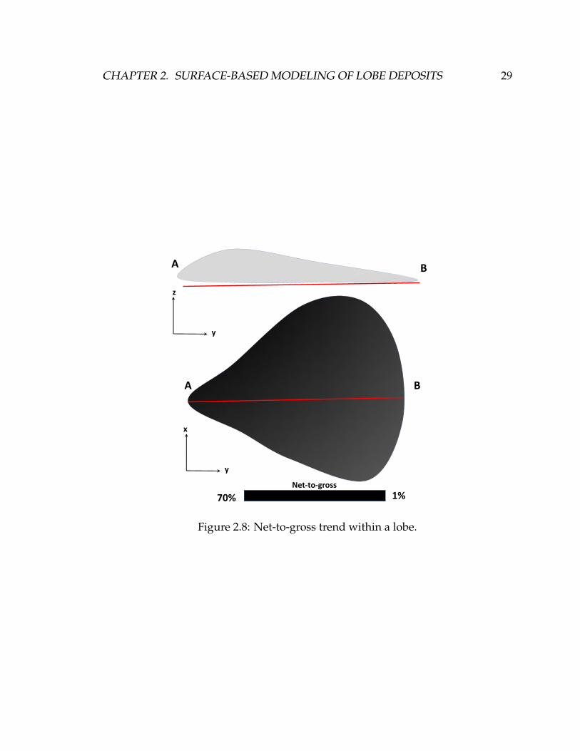
CHAPTER 2. SURFACE-BASED MODELING OF LOBE DEPOSITS 29
A B
A B
Net-to-gross
70% 1%
y
x
y
z
Figure 2.8: Net-to-gross trend within a lobe.
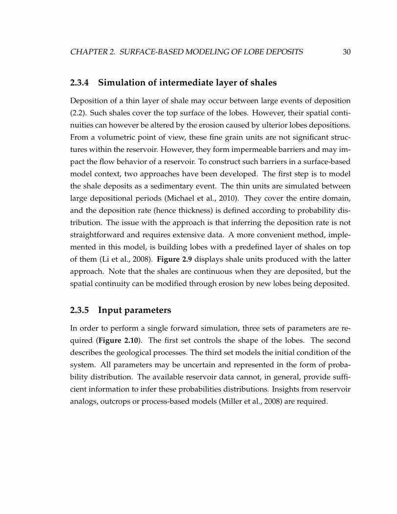
CHAPTER 2. SURFACE-BASED MODELING OF LOBE DEPOSITS 30
2.3.4 Simulation of intermediate layer of shales
Deposition of a thin layer of shale may occur between large events of deposition
(2.2). Such shales cover the top surface of the lobes. However, their spatial conti-
nuities can however be altered by the erosion caused by ulterior lobes depositions.
From a volumetric point of view, these fine grain units are not significant struc-
tures within the reservoir. However, they form impermeable barriers and may im-
pact the flow behavior of a reservoir. To construct such barriers in a surface-based
model context, two approaches have been developed. The first step is to model
the shale deposits as a sedimentary event. The thin units are simulated between
large depositional periods (Michael et al., 2010). They cover the entire domain,
and the deposition rate (hence thickness) is defined according to probability dis-
tribution. The issue with the approach is that inferring the deposition rate is not
straightforward and requires extensive data. A more convenient method, imple-
mented in this model, is building lobes with a predefined layer of shales on top
of them (Li et al., 2008). Figure 2.9 displays shale units produced with the latter
approach. Note that the shales are continuous when they are deposited, but the
spatial continuity can be modified through erosion by new lobes being deposited.
2.3.5 Input parameters
In order to perform a single forward simulation, three sets of parameters are re-
quired (Figure 2.10). The first set controls the shape of the lobes. The second
describes the geological processes. The third set models the initial condition of the
system. All parameters may be uncertain and represented in the form of proba-
bility distribution. The available reservoir data cannot, in general, provide suffi-
cient information to infer these probabilities distributions. Insights from reservoir
analogs, outcrops or process-based models (Miller et al., 2008) are required.

CHAPTER 2. SURFACE-BASED MODELING OF LOBE DEPOSITS 31
Proximal
Distal
J=76J=88
J=102
Process-based model Surface-based model
Figure 2.9: Comparison of cross-sections of the process-based model (on the left)and a surface-based model (on the right) for a small lobe system. The top picturesrepresent the entire sedimentary structure. The bottom one shows only the shalelayers. We observe that surface-based models can reproduce sedimentary struc-tures that are realistic when compared to process-based models, but at a fractionof the CPU-costs. Courtesy from Li (Li et al., 2008)

CHAPTER 2. SURFACE-BASED MODELING OF LOBE DEPOSITS 32
Parameters and rules Representation Uncertainty
Lobe
geometry
-Template geometry Deterministic
equation
Uncertain because inferred
from analog models and/or
data. The lobe geometry is
modified by an erosion process
that is difficult to quantify.
-Width CDF
-Length CDF
-Thickness CDF
-Variance/Covariance of the
perturbation
CDF
Geological
process
-Progradation intensity CDF
Abstraction of complex
physical processes into
simplified rules leads to an
additional error or
uncertainty. The statistics are
inferred from process-based
models analysis.
-Migration intensity CDF
- Influence of topography on
deposition
Deterministic
set of rules
-Tau value CDF
-Frequency of intermediate shale Deterministic
set of rules
-Erosion intensity
Deterministic
set of rules
-Number of lobes CDF
Initial
condition
-Coordinates X Y of the
sediments source
CDF
Uncertain because this location
is not recorded in any
geological structures, there can
be multiple sources including
those outside the domain of
study
Figure 2.10: Summary of the rules and parameters needed to run a simulation (seealso Michael et al. (2010)). The parameters are highly uncertain because they aredifficult to infer. They are represented in the form of probability distributions.To generate a realization, the parameter values are drawn from these probabilitydistributions. (CDF=cumulative density function).

CHAPTER 2. SURFACE-BASED MODELING OF LOBE DEPOSITS 33
Figure 2.11: Gridding of a lobe. Stratigraphic grids can be built from the surfacesgenerated by the surface-based algorithm. This grid serves as a support for prop-erties characterization.
2.3.6 Surface-based model output
At the end of a forward simulation, the algorithm outputs a thickness map of each
deposited lobe. By stacking them on top of each others, a 3D model of the reservoir
discontinuities is created. These surfaces are used to build a stratigraphic grid
(Figure 2.11). The petrophysical properties defined during the forward simulation
can then be mapped onto this grid.
2.4 Summary of the chapter
Surface-based models generate reservoir geometries and heterogeneities by mim-
icking sedimentary processes. A critical step after developing such a model is
to validate the geological consistency of the generated realizations. In this case,
their realism has been evaluated by Michael et al. (2010). Reservoir geometries
generated by the surface-based model were compared with reservoir geometries
generated by a process-based model. The process-based heterogeneities, because

CHAPTER 2. SURFACE-BASED MODELING OF LOBE DEPOSITS 34
they are highly detailed, were considered as a reference. The study showed that the
features produced by the surface-based model compare well with those of process-
based ones. Such analysis proves that our algorithm can produce realistic reservoir
structures. However, in order to predict accurately the structures of a particular
reservoir, the surface-based model, in addition to being geologically consistent,
should also account for any available data.

Chapter 3
Framework for data conditioning
3.1 Motivation
Models are used as input in flow simulators to obtain, for example, cumulative
oil productions under a given field development scenario. Drilling wells is costly
in the deep-water environment, and engineers need models to represent what the
reservoir can look like to optimize a well path. Hence, building an accurate repre-
sentation of the reservoir is primordial. However, the exact reservoir architecture
is unknown because exhaustively sampling the reservoir is impossible. Yet, some
knowledge of the structure is available. First, measurements of the reservoir struc-
ture exist: geophysics survey, well logs, production history, well test... Secondly,
the model of continuity inside the reservoir is generally known: type of sedimen-
tary structures, their relationship, etc. Such prior geological knowledge is obtained
by linking the regional geological setting with reservoir analogs, outcrop studies or
process-based models. In order to model as accurately as possible the reservoir un-
der assessment, one must take the prior geological knowledge into account. In the
case of lobe deposits, surface-based models provide a tool for generating models
that honor such prior geological knowledge. The models should also account for
the information extracted from the reservoir data. However, a randomly selected
surface-based model has few chances to match the actual observations. Hence, one
should find a way to create surface-based models that match the available data.
35

CHAPTER 3. FRAMEWORK FOR DATA CONDITIONING 36
3.1.1 Challenges of conditioning surface-based models to data
The actual approaches developed for matching data are based on a direct (non-
iterative) constraint to the data. The first approach, developed by Pyrcz et al.
(2004), fits the neighboring well data by locally adjusting the lobe surface. When
the surface geometry contradicts data outside a tolerance, the location of the lobe
is modified to achieve a match. The second approach proposed by Zhang et al.
(2009) achieves a a match with wells by direct interpolation between logs. A large
amount of wells is required, which is unrealistic in deep offshore development.
Furthermore, using interpolation to match well data entails the risk of modifying
in an unrealistic way the shape of the lobes. The generated surface-based model
may not be consistent with the prior geological knowledge that has been defined.
The last method, developed by Michael et al. (2010), obtains a match with well
data conditioning using well correlation. Each of the depositional units needs to
be identified in well data and ordered according to the different depositional peri-
ods. However, interpreting wells in such a detailed fashion is time-consuming and
subject to uncertainty.
A general conditioning method is to identify the model parameters that pro-
duces numerical simulations matching the data. The problem can be handled us-
ing inverse theory (Tarantola, 2005). Inversion is a rigorous method to system-
atically search for numerical simulations that match the data by iterating on the
model input. Since the numerical simulations are not artificially modified to match
the data, the model geological consistency is preserved. By matching data and be-
ing geologically consistent, one hopes the model has some predictability abilities.
Obtaining a set of matching models provides a model of uncertainty. The ability
to assess uncertainty and risks makes inverse modeling particularly suitable for
reservoir modeling. In earth-modeling, the concept of data integration through
inverse modeling is tackled either via sampling (Bayesian framework) or via opti-
mization.
CHAPTER 3. FRAMEWORK FOR DATA CONDITIONING 37
3.1.2 Sampling approach to inverse modeling
To determine the population of models that match data, one approach is to exhaus-
tively sample the parameters distributions in order to generate a large number of
models, and to reject the models that do not honor the data. This approach, termed
rejection sampling (von Neumann, 1951) allows modeling realistically the uncer-
tainty for the future predictions. However, this requires an enormous amount of
iterations, making it impossible to use in practice. Other more efficient, but less ac-
curate sampling techniques exist. One widely used technique is the Markov Chain
Monte Carlo technique, a stochastic sampling-based approach (MCMC, Gilks et al.
(1996) ). MCMC algorithms aim at constructing a random walk to sample the
parameter space. The difference with a rejection sampler is that the sampling of
a new model is not random but conditional on where the sampler was the step
before (Markov Chain). Using a sampling technique has not been investigated
in surface-based modeling. The methods, however, have been applied in inverse
stratigraphic modeling (Bornholdt et al., 1999; Cross and Lessenger, 1999; Charvin
et al., 2009). Inverse stratigraphic modeling is similar in nature to reservoir model-
ing, except the subject of interest is a basin and not a reservoir, and the purpose of
the study is not evaluating the risks of developing a field, but extracting some geo-
logical parameters, such as sea level change, sediment supply or basin topography
from stratigraphic data. The computational-costs associated with these methods
,however, remains a problem . In Charvin et al. (2009), the study aims to quantify
the full ranges of sediment supply and sea level variation that have generated sed-
imentary structures observed in 6 wells. The inverse modeling is handled using
a MCMC approach. To minimize the computational costs, the inverse model is
combined with a simple 2D forward model, controlled by 15 parameters. The data
were not real and simulated with the same forward model used to solve the prob-
lem. Despite the apparent simplicity of the inverse problem, 65000 iterations are
required to define accurately the posterior distribution. In the context of surface-
based modeling , the model is 3D, the data are of different nature, and the number
of parameters to update can be up to one hundred. Hence, solving the full inverse
CHAPTER 3. FRAMEWORK FOR DATA CONDITIONING 38
problem rigorously, even by using an efficient sampler, is not convenient.
3.1.3 Optimization approach to inverse modeling
Alternatively to rigorously solving the inverse problem by sampling, one can look
to optimization techniques to find sets of matched models. However, Such tech-
nique do not guarantee the full exploration of the parameter-space; the algorithms
can indeed favor some particular combinations of parameters because they are
easiest to find. Indeed, optimization approaches typically produce a set of models
that have much smaller uncertainty than the one obtained from sampling. In other
words, the generated models resemble each other more closely.
Yet, optimization may be the only way to find models that match the data with a
reasonable CPU-time. Optimization has been investigated in inverse stratigraphic
modeling. Bornholdt et al. (1999) propose a method based on genetic algorithms.
The case study presented in the paper is relatively simple: a 2D forward model,
2 synthetic wells and 7 parameters to optimize. Still, at least 1000 forward model
runs were required to generate a model having a fair resemblance to the data.
In the context of surface-based modeling, the problems are too complex and the
model too highly parameterized to be applied successfully within traditional opti-
mization approaches. Thus, we propose a new optimization framework, based on
a divide-and-conquer approach.
3.2 Conditioning of a surface-based model through op-
timization
3.2.1 Problem statement
Surface-based models contain two stochastic components (Figure 3.2). The first
one randomly selects the input parameters values from probability distributions:
size of the lobes, source locations, etc. It models the uncertainty of the input pa-
rameters values. Additionally, some of these input parameters define the model

CHAPTER 3. FRAMEWORK FOR DATA CONDITIONING 39
Spatial uncertaintyParameters uncertainty Output variability
Possible lobe locations for a
same set of parameters
?
Figure 3.1: Surface-based models present two stochastic processes. The first oneis due to input parameter uncertainty. To run a simulation, input values are ran-domly drawn from probability distributions. Some of these parameters are thenused to define a probability map of lobe locations. This represents the spatial un-certainty; a set of input parameters only narrows the possible locations of a lobeover the domain, and the exact location is randomly selected from this probabilitymap. Both of those stochastic processes control the output variability.
CHAPTER 3. FRAMEWORK FOR DATA CONDITIONING 40
of deposition and are used to compute a probability map of lobe locations. The
exact locations of the lobes are then drawn from this probability map. This second
stochastic process models the spatial uncertainty, which is the uncertainty on lobes
locations given a specific set of input parameters values.
In inverse modeling, one attempts to create 3D models that match the data
by varying both the input parameters and the spatial locations of the geological
structures. Solving such inverse problem by means of optimization is not straight-
forward. Since the deposition of each geobody requires defining a new set of pa-
rameters values and spatial locations, the total number of parameters to optimize
becomes rapidly prohibitive. For a simple model containing ten lobes, each lobe
being specified by three parameters, the optimization problem involves thirty pa-
rameters. This number does not yet account for the parameters controlling the
geological process and the parameters setting the initial condition of the system.
Decreasing the number of parameters is therefore vital to develop an efficient op-
timization scheme. Three complementary approaches are investigated to address
this challenge: an evaluation of the impact of spatial uncertainty versus parameter
uncertainty, a sensitivity analysis of the input parameters and a reformulation of
the optimization problem.
3.2.2 Evaluating parameter uncertainty versus spatial uncertainty
Determining the parameters impacting the data-fit is essential because, once iden-
tified, one can focus on optimizing them and ignore the less impacting ones. Such
model simplification makes the computational burden of optimization more sup-
portable.
The first step is then to study the sensitivity of the model to families of pa-
rameters. In our surface-based model, two families of parameters exist. The first
family contains the model input parameters: lobe size, source location, etc. The
second family contains the spatial parameters, which are the lobes locations. For
both families, the parameter values are uncertain: hence, one refers to parame-
ter uncertainty and spatial uncertainty. The first step of the sensitivity analysis is
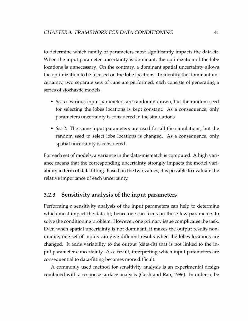
CHAPTER 3. FRAMEWORK FOR DATA CONDITIONING 41
to determine which family of parameters most significantly impacts the data-fit.
When the input parameter uncertainty is dominant, the optimization of the lobe
locations is unnecessary. On the contrary, a dominant spatial uncertainty allows
the optimization to be focused on the lobe locations. To identify the dominant un-
certainty, two separate sets of runs are performed; each consists of generating a
series of stochastic models.
• Set 1: Various input parameters are randomly drawn, but the random seed
for selecting the lobes locations is kept constant. As a consequence, only
parameters uncertainty is considered in the simulations.
• Set 2: The same input parameters are used for all the simulations, but the
random seed to select lobe locations is changed. As a consequence, only
spatial uncertainty is considered.
For each set of models, a variance in the data-mismatch is computed. A high vari-
ance means that the corresponding uncertainty strongly impacts the model vari-
ability in term of data fitting. Based on the two values, it is possible to evaluate the
relative importance of each uncertainty.
3.2.3 Sensitivity analysis of the input parameters
Performing a sensitivity analysis of the input parameters can help to determine
which most impact the data-fit; hence one can focus on those few parameters to
solve the conditioning problem. However, one primary issue complicates the task.
Even when spatial uncertainty is not dominant, it makes the output results non-
unique; one set of inputs can give different results when the lobes locations are
changed. It adds variability to the output (data-fit) that is not linked to the in-
put parameters uncertainty. As a result, interpreting which input parameters are
consequential to data-fitting becomes more difficult.
A commonly used method for sensitivity analysis is an experimental design
combined with a response surface analysis (Gosh and Rao, 1996). In order to be

CHAPTER 3. FRAMEWORK FOR DATA CONDITIONING 42
efficient, such methods requires models that vary relatively smoothly with regard
to the input parameters, which is not the cased of surface-based models.
Instead, a distance-based model selection and sensitivity analysis is applied.
This method has been successfully applied by Scheidt and Caers (2009) to study
the sensitivity of a reservoir flow behavior in term of channel characteristics. The
key idea behind this method is to define a dissimilarity distance between simu-
lated models. This distance indicates how similar two models are in terms of the
response of interest (in our case, the data-fit). Based on these dissimilarities, the
models are mapped in a low dimensional space, where clustering is applied. Such
mapping facilitates extraction of the underlying structure and relations between
models. Each cluster consists, therefore, of models with similar characteristics. For
each cluster, one can define the subset of parameters values used to generate the
models. By studying how these subsets compare to each other, it is possible to
identify the most influential parameters.
Algorithm 3.2.1 Distance-based sensitivity analysis1) Simulate a set of surface-based models by varying the input parameters (parameteruncertainty) and, for each set of input parameters, the location of the geobodies (spatialuncertainty).2) Compute the distance between each generated models. If n models have been gener-ated, the dimension of the matrix is n*n. The distance is based on the mismatch with thedata.3) Using the distance, the surface-based models are projected in the MDS space.4) The points are mapped in the kernel space, using kernel transformation.5) K-means clustering is applied to the set models; each cluster gathers models withsimilar misfit.6) Select the surface-based models closest to the cluster centers.7) Evaluate the joint variation of parameters within a cluster and between clusters toidentify the leading parameters.
3.3 Optimization
Once the sensitive parameters have been identified, the following step consists of
optimizing them. To perform this step efficiently, three issues must be addressed.
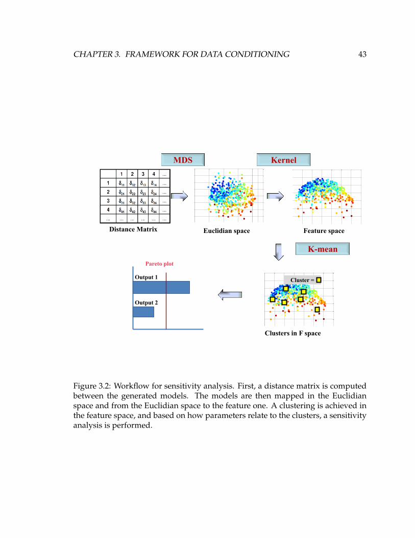
CHAPTER 3. FRAMEWORK FOR DATA CONDITIONING 43
-10 -5 0 5 10-10010
-8
-6
-4
-2
0
2
4
6
8
Distance Matrix
MDS
0.1413
0.1413
0.1413
0.1413
0.1413
0.1413
0.1413
0.1413
-0.4-0.3-0.2-0.100.10.20.3
0.1413
0.1413
0.1413
0.1413
0.1413
0.1413
0.1413
0.1413
-0.4-0.3-0.2-0.100.10.20.3
K-mean
Pareto plot
Output 1
Output 2
Kernel
Euclidian space Feature space
Clusters in F space
Cluster =
Figure 3.2: Workflow for sensitivity analysis. First, a distance matrix is computedbetween the generated models. The models are then mapped in the Euclidianspace and from the Euclidian space to the feature one. A clustering is achieved inthe feature space, and based on how parameters relate to the clusters, a sensitivityanalysis is performed.

CHAPTER 3. FRAMEWORK FOR DATA CONDITIONING 44
First, the model response is non-smooth to input variations. Secondly, the Gaus-
sian noise perturbing the lobes thicknesses must respond smoothly to input pa-
rameters changes. Lastly, the number of parameters to be optimized can be signif-
icant, resulting in prohibitive computational-costs. Each problem is addressed in
the following paragraphs.
3.3.1 Choice of the optimization algorithm
The aim of an optimization approach is to find efficiently parameters (input pa-
rameters and/or lobes locations) that generate matched models. Surface-based
models do not respond smoothly to small variations in the parameters. Conse-
quently, discontinuities in the response function exist. Gradient-based optimiza-
tion techniques are inefficient to solve this conditioning problem. Instead, find-
ing a solution requires a direct-search optimization techniques that do not need to
compute the response function gradient (Hooke and Jeeves, 1961). Direct-search
methods optimize a problem by iteratively sampling the search-space. The sam-
pling is not random but based on a strategy that determines the new sample from
results of the previous iterations. Several strategies exist to explore efficiently the
parameter-space: Genetic Algorithm, Particle Swarm, Simulating Annealing, etc.
In this work, the Nelder-Mead approach (polytope method) is chosen due to its
simplicity and its robustness for problems with discontinuities (Nelder and Mead,
1965).
The Nelder-Mead algorithm uses n + 1 point in Rn. These points create a poly-
tope, which is a generalization of a polygon in an n dimensional space: a triangle
in R2, a tetrahedron in R3, etc. The goal of Nelder-Mead optimization is to replace
the worst vertex of the simplex, which is the candidate having the worst data-fit,
with a better one. As a consequence, the vertices of the simplex are modified in an
intelligent manner so that the simplex can converge to a minimum (Figure 3.3).

CHAPTER 3. FRAMEWORK FOR DATA CONDITIONING 45
Algorithm 3.3.1 Nelder-Mead1) Creation of a sample of n + 1 points in Rn .2) The n + 1 points are ordered according to their corresponding objective values, fromthe best F[0] to the worst F[n].3) The center m of the n best points is computed.4) A new point r is obtained from reflecting the worst point F[n] through m.5) If the new point r is neither better than F[0] or not as worse as F[n], F[n] is replacedby m.6) If the new point r is better than the best solution candidate F[0], the simplex isexpanded to this promising region.7) If the new point r is worst than F[n], the simplex is contracted by creating a pointbetween r and m.
F[1]
F[2]F[0]
R
M
F[1]
F[2]F[0]
M
R
E
F[1]
F[0]
R
M
C
F[2]
F[1]
F[0] F[2]F[2’]
F[1’]
Reflection Expansion Contraction Shrinking
Figure 3.3: Possible modifications of a simplex applied to a problem in two dimen-sions.
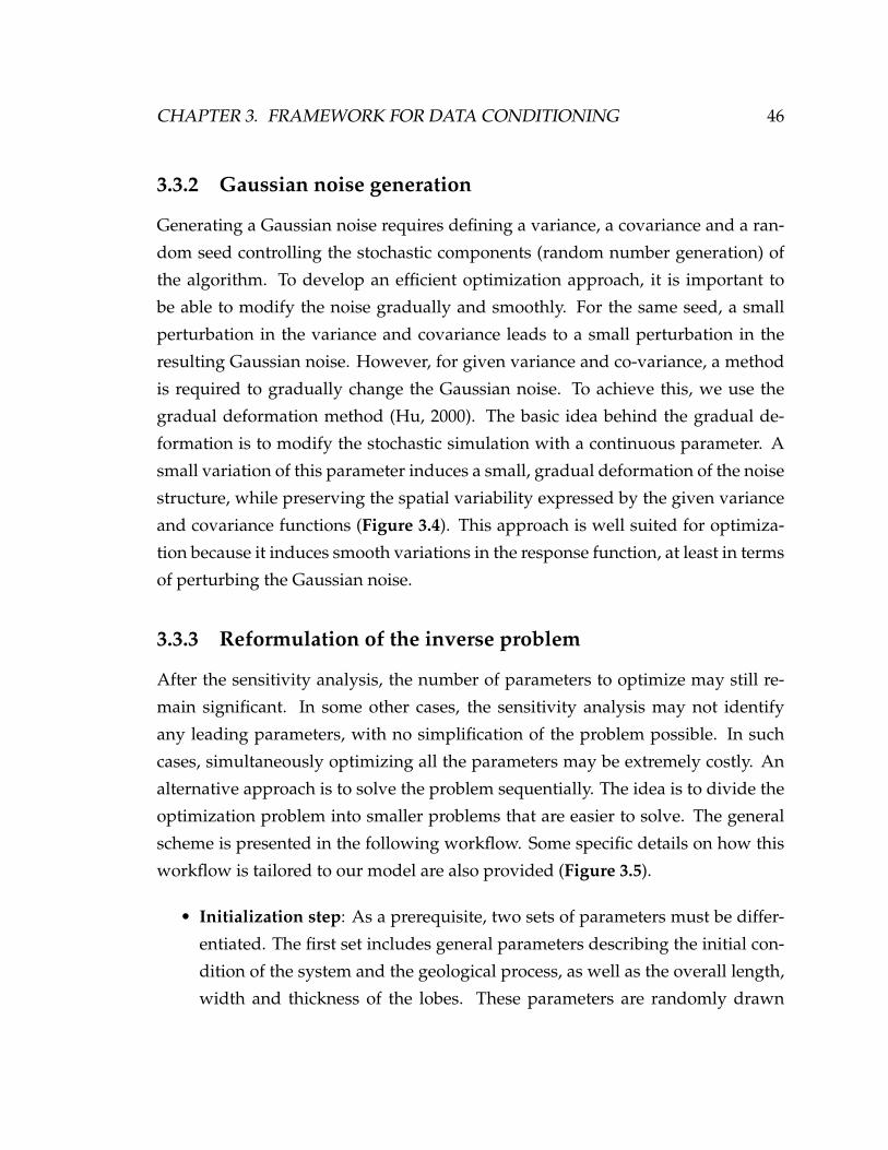
CHAPTER 3. FRAMEWORK FOR DATA CONDITIONING 46
3.3.2 Gaussian noise generation
Generating a Gaussian noise requires defining a variance, a covariance and a ran-
dom seed controlling the stochastic components (random number generation) of
the algorithm. To develop an efficient optimization approach, it is important to
be able to modify the noise gradually and smoothly. For the same seed, a small
perturbation in the variance and covariance leads to a small perturbation in the
resulting Gaussian noise. However, for given variance and co-variance, a method
is required to gradually change the Gaussian noise. To achieve this, we use the
gradual deformation method (Hu, 2000). The basic idea behind the gradual de-
formation is to modify the stochastic simulation with a continuous parameter. A
small variation of this parameter induces a small, gradual deformation of the noise
structure, while preserving the spatial variability expressed by the given variance
and covariance functions (Figure 3.4). This approach is well suited for optimiza-
tion because it induces smooth variations in the response function, at least in terms
of perturbing the Gaussian noise.
3.3.3 Reformulation of the inverse problem
After the sensitivity analysis, the number of parameters to optimize may still re-
main significant. In some other cases, the sensitivity analysis may not identify
any leading parameters, with no simplification of the problem possible. In such
cases, simultaneously optimizing all the parameters may be extremely costly. An
alternative approach is to solve the problem sequentially. The idea is to divide the
optimization problem into smaller problems that are easier to solve. The general
scheme is presented in the following workflow. Some specific details on how this
workflow is tailored to our model are also provided (Figure 3.5).
• Initialization step: As a prerequisite, two sets of parameters must be differ-
entiated. The first set includes general parameters describing the initial con-
dition of the system and the geological process, as well as the overall length,
width and thickness of the lobes. These parameters are randomly drawn

CHAPTER 3. FRAMEWORK FOR DATA CONDITIONING 47
10 20 30 40 50 60 70 80 90 100
10
20
30
40
50
60
70
80
90
100
10 20 30 40 50 60 70 80 90 100
10
20
30
40
50
60
70
80
90
100
10 20 30 40 50 60 70 80 90 100
10
20
30
40
50
60
70
80
90
100
Co
effi
cie
nt
for
the
gra
du
al d
efo
rmat
ion
T=1
T=2
T=3
Figure 3.4: Traditionally, a Gaussian noise is generated by defining a variance,covariance and seed. This seed controls the stochastic component of the algorithm.In terms of optimization, generating a noise using this approach is not convenientbecause a small perturbation of the seed completely changes the noise structure,inducing discontinuities in the objective function. Generating a Gaussian noiseusing the gradual deformation method avoids this issue (Hu, 2000). Thanks to thismethod, the stochastic process is controlled by a continuous parameter and nota random seed; a small change in this parameter generates a slight deformationof the noise, thus causing a smooth variation in the objective function in terms ofperturbing the Gaussian noise.
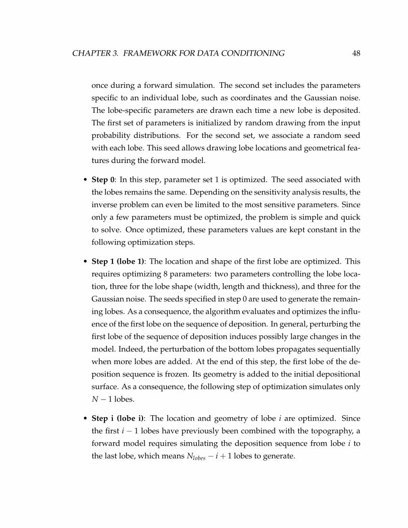
CHAPTER 3. FRAMEWORK FOR DATA CONDITIONING 48
once during a forward simulation. The second set includes the parameters
specific to an individual lobe, such as coordinates and the Gaussian noise.
The lobe-specific parameters are drawn each time a new lobe is deposited.
The first set of parameters is initialized by random drawing from the input
probability distributions. For the second set, we associate a random seed
with each lobe. This seed allows drawing lobe locations and geometrical fea-
tures during the forward model.
• Step 0: In this step, parameter set 1 is optimized. The seed associated with
the lobes remains the same. Depending on the sensitivity analysis results, the
inverse problem can even be limited to the most sensitive parameters. Since
only a few parameters must be optimized, the problem is simple and quick
to solve. Once optimized, these parameters values are kept constant in the
following optimization steps.
• Step 1 (lobe 1): The location and shape of the first lobe are optimized. This
requires optimizing 8 parameters: two parameters controlling the lobe loca-
tion, three for the lobe shape (width, length and thickness), and three for the
Gaussian noise. The seeds specified in step 0 are used to generate the remain-
ing lobes. As a consequence, the algorithm evaluates and optimizes the influ-
ence of the first lobe on the sequence of deposition. In general, perturbing the
first lobe of the sequence of deposition induces possibly large changes in the
model. Indeed, the perturbation of the bottom lobes propagates sequentially
when more lobes are added. At the end of this step, the first lobe of the de-
position sequence is frozen. Its geometry is added to the initial depositional
surface. As a consequence, the following step of optimization simulates only
N − 1 lobes.
• Step i (lobe i): The location and geometry of lobe i are optimized. Since
the first i − 1 lobes have previously been combined with the topography, a
forward model requires simulating the deposition sequence from lobe i to
the last lobe, which means Nlobes − i + 1 lobes to generate.
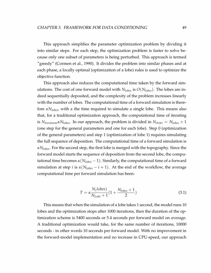
CHAPTER 3. FRAMEWORK FOR DATA CONDITIONING 49
This approach simplifies the parameter optimization problem by dividing it
into similar steps. For each step, the optimization problem is faster to solve be-
cause only one subset of parameters is being perturbed. This approach is termed
”greedy” (Cormen et al., 1990). It divides the problem into similar phases and at
each phase, a locally optimal (optimization of a lobe) rules is used to optimize the
objective function.
This approach also reduces the computational time taken by the forward sim-
ulations. The cost of one forward model with Nlobes is O(Nlobes). The lobes are in-
deed sequentially deposited, and the complexity of the problem increases linearly
with the number of lobes. The computational time of a forward simulation is there-
fore αNlobes, with α the time required to simulate a single lobe. This means also
that, for a traditional optimization approach, the computational time of iterating
is NiterationsαNlobes. In our approach, the problem is divided in Nsteps = Nlobes + 1
(one step for the general parameters and one for each lobe). Step 0 (optimization
of the general parameters) and step 1 (optimization of lobe 1) requires simulating
the full sequence of deposition. The computational time of a forward simulation is
αNlobes. For the second step, the first lobe is merged with the topography. Since the
forward model starts the sequence of deposition from the second lobe, the compu-
tational time becomes α(Nlobes− 1). Similarly, the computational time of a forward
simulation at step i is α(Nlobes − i + 1). At the end of the workflow, the average
computational time per forward simulation has been:
T = αN(lobes)NLobe + 1
(1 +Nlobes + 1
2) (3.1)
This means that when the simulation of a lobe takes 1 second, the model runs 10
lobes and the optimization stops after 1000 iterations, then the duration of the op-
timization scheme is 5400 seconds or 5.4 seconds per forward model on average.
A traditional optimization would take, for the same number of iterations, 10000
seconds - in other words 10 seconds per forward model. With no improvement in
the forward-model implementation and no increase in CPU-speed, our approach

CHAPTER 3. FRAMEWORK FOR DATA CONDITIONING 50
allows performing almost twice as many forward simulations as a typical opti-
mization approach does during the exact same computational time.
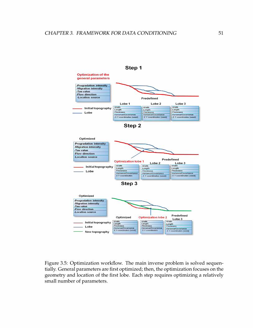
CHAPTER 3. FRAMEWORK FOR DATA CONDITIONING 51
Figure 3.5: Optimization workflow. The main inverse problem is solved sequen-tially. General parameters are first optimized; then, the optimization focuses on thegeometry and location of the first lobe. Each step requires optimizing a relativelysmall number of parameters.
CHAPTER 3. FRAMEWORK FOR DATA CONDITIONING 52
3.4 Discussion and conclusion
In this chapter, we presented a workflow that allows for the generation of surface-
based models conditioned to data. The workflow is based on an optimization of
the model parameters. Since solving such optimization problems is computation-
ally costly, the key idea behind the method is to decrease the dimensionality of
the problem. To this end, three complementary approaches are developed. The
first one identifies the leading uncertainty. The second one is a sensitivity analy-
sis of the input parameters. The third one is a reformulation of the optimization
problem. The problem is then solved sequentially and not simultaneously. This re-
formulation, by decreasing the number of lobes to simulate after each optimization
sequence, also reduces the cost of running the model. The workflow is general in
the sense that it can be applied in theory to any type of data and environments of
deposition. However, this conditioning methodology raises two main limitations.
The first problem to consider is the possible difficulty of finding matching mod-
els when a large amount of data is available. If data are too constraining, finding
solutions may indeed be an extremely slow process. The presented conditioning
method is therefore more suitable for problems with few data, a common situation
in the early stage of reservoir development. Since surface-based models have been
primarily developed for early stage reservoir development too, the limitations of
the conditioning method do not affect its applicability for real-world problems.
A second problem to consider is the relevance of the optimization approach
when assessing uncertainties. Conditional models are generated for their predic-
tive abilities. With surface-based models, the conditioning problem is ill-posed.
This means that different matched models can be generated, and uncertainty in
the model predictions exists. When making decisions, it is critical to account for
all the possible predictions. This requires an extremely costly sampling of the pa-
rameters distributions. With an optimization approach, matched models are gen-
erated more efficiently. However, the parameters space may not be exhaustively
explored, and some matched models may be ignored, which can bias the decisions
made in terms of reservoir development. This problem is investigated at the end

CHAPTER 3. FRAMEWORK FOR DATA CONDITIONING 53
of Chapter 6.

Chapter 4
Application to the East-Breaks dataset
4.1 Introduction
In the previous chapter, an approach for conditioning surface-based models to
reservoir data was described. In this chapter, the approach is tested on a real
dataset named East-Breaks, composed of a thickness map and wells data. East-
Breaks provides an excellent scenario for evaluating the method applicability in
early stage reservoir development; a seismic survey is available, but few wells
have been drilled and no production data exists. The focus of the test case is to
evaluate the method applicability and computational efficiency. In other words,
the end goal is not to show that a perfect data-fit can be obtained regardless of the
computational cost, but rather to demonstrate that a good mach can be achieved
in a reasonable time frame.
4.2 The data-set
The workflow is applied to a real data set originating from a Pleistocene turbidite
system in the East Breaks mini-basin, West of Gulf of Mexico (Miller et al., 2008).
This mini-basin is 8 km wide by 16 km long and is filled with lobe deposits Fig-
ure 4.1. The data are composed of 3 well logs and 2 surfaces (the bottom and top
surfaces of the mini-basin). The log data provides information about thicknesses of
54
CHAPTER 4. APPLICATION TO THE EAST-BREAKS DATASET 55
individual lobes at the wells locations. Because the mini-basin is very shallow, we
assume that the morphology of the surfaces does not need any restoration. As a
consequence, the bottom surface is used directly as the paleo-seafloor on which the
simulated lobes are deposited. The top surface is then used to compute the thick-
ness map of the sediments. The log data and thickness map are consistent with
each other in the sense that the sum of all the lobes thicknesses recorded in a well
matches the corresponding thickness defined in the map. In a traditional reser-
voir study, surfaces, also called horizons, are derived from a seismic survey, and
individual lobes thicknesses are deduced from well logging measurements. The
data used in the case study are not raw seismic data but have been processed and
interpreted; they are therefore subject to uncertainty. The data uncertainty plays
a critical role in problems where risks in exploration, development or production
of reservoirs must be assessed (Thore et al., 2002). In general, such uncertainty is
handled by working on different alternative data sets. In other words, considering
data uncertainty in our particular optimization scheme would require generating
top surface models for each of the alternative data sets. In our study, we assume
we are dealing with one such top surface, or one alternative thickness data set.
The case study is twofold. First, the workflow is applied to generate a surface-
based model that fits the East-Breaks wells and thickness data. Next, the compu-
tational performance of the method is evaluated. The main challenge brought by
East-Breaks is caused by the different types of data: matching the thickness map
means reproducing the overall shape of the sediments package. Matching log data
requires reproducing a precise internal layering at the well locations.
4.3 Specification of the input parameters
In our model, the geological process and the initial condition of the system are de-
fined by seven parameters, such as source location or progradation intensity, etc.
Each lobe is, in addition, defined by eight parameters: three for the lobe shape
(length, thickness and width), two for the lobe location, and three for the Gaussian
noise generation. These parameters are uncertain and represented with probability
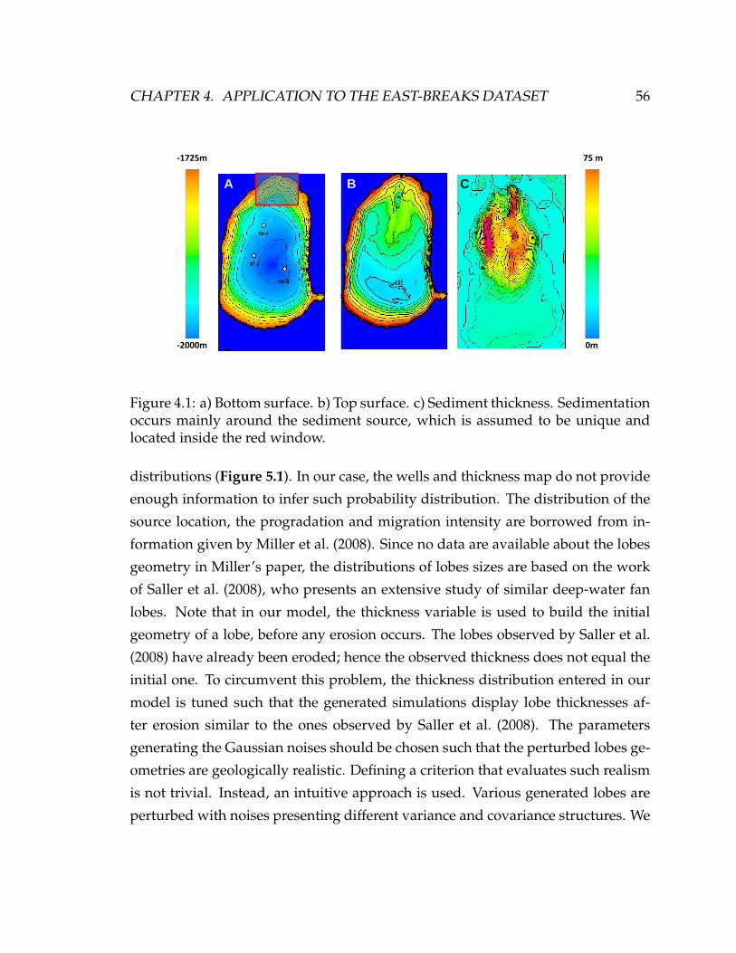
CHAPTER 4. APPLICATION TO THE EAST-BREAKS DATASET 56
-2000m
-1725m
0m
75 m
A B C
Figure 4.1: a) Bottom surface. b) Top surface. c) Sediment thickness. Sedimentationoccurs mainly around the sediment source, which is assumed to be unique andlocated inside the red window.
distributions (Figure 5.1). In our case, the wells and thickness map do not provide
enough information to infer such probability distribution. The distribution of the
source location, the progradation and migration intensity are borrowed from in-
formation given by Miller et al. (2008). Since no data are available about the lobes
geometry in Miller’s paper, the distributions of lobes sizes are based on the work
of Saller et al. (2008), who presents an extensive study of similar deep-water fan
lobes. Note that in our model, the thickness variable is used to build the initial
geometry of a lobe, before any erosion occurs. The lobes observed by Saller et al.
(2008) have already been eroded; hence the observed thickness does not equal the
initial one. To circumvent this problem, the thickness distribution entered in our
model is tuned such that the generated simulations display lobe thicknesses af-
ter erosion similar to the ones observed by Saller et al. (2008). The parameters
generating the Gaussian noises should be chosen such that the perturbed lobes ge-
ometries are geologically realistic. Defining a criterion that evaluates such realism
is not trivial. Instead, an intuitive approach is used. Various generated lobes are
perturbed with noises presenting different variance and covariance structures. We

CHAPTER 4. APPLICATION TO THE EAST-BREAKS DATASET 57
reject then the lobes whose shapes are not recognizable anymore after perturba-
tion. As a result, we estimate that the noise correlation length should be between
1000m and 7000m for all lobes. The variance is more critical because it defines the
roughness of the perturbed surface and has a larger impact on the lobe overall ge-
ometry, hence consistency. The maximum variance is defined such that the created
perturbation does not exceed (in thickness units) one third of the maximum lobe
thickness.
Running the above-defined forward model also requires defining the number
of lobes present in the system. This number is important because it functions as a
stopping criterion for the model; the forward simulation ends when the specified
number of deposited lobes is reached. In our case study, we decide to use a differ-
ent stopping criterion. Indeed, the thickness map gives information on the volume
of deposited sediments, not the number of lobes. Therefore, a forward simulation
stops when the volume of deposited lobes matches the reference volume. Defin-
ing the number of lobes is thus unnecessary. Due to the lack of data describing
the East-Breaks system, the input parameters are highly uncertain and their asso-
ciated probability distributions present a large range of variability. This may result
in a slower convergence towards matching the well and thickness data since the
search-space is relatively large.

CHAPTER 4. APPLICATION TO THE EAST-BREAKS DATASET 58
Parameters Distribution
Lobe
Geometry
Width Uniform [1000m 3000m]
Length Uniform [2000m 7000m]
Thickness Uniform [5m 35m]
Variance of the noise Uniform [0 x]
x depending on the maximum lobe thickness
Covariance of the noise Uniform [1000m 7000m]
Geological
process
Progradation intensity Uniform [500m 1000m]
Migration intensity Uniform [200m 700m]
Tau value Uniform [0 1]
Initial
condition
Coordinates X Y of the
sediments source
Unique and uniformly distributed in a window of
3kms by 3kms situated at the top of the domain.
Table 4.1: Probability distributions associated with the input parameters.
4.4 Definition of the objective function
An objective function determines how close a model is in reaching the objective of
the optimization. In the case study, a matched model should fit the thickness map
and the log data simultaneously. This corresponds to two sub-objectives. Similarly,
matching the log data requires matching the lobes thicknesses recorded in each of
the three logs.
Ewelli =a
Nlobes data
Nlobes data
∑1
(thick data lobei − thick sim lobei)2 (4.1)
The result is a mean square error of the mismatch in terms of lobe thickness.
The errors associated with each well are then averaged to obtain a combined wells
error Ewells.

CHAPTER 4. APPLICATION TO THE EAST-BREAKS DATASET 59
Ewells =13
3
∑1
Ewelli (4.2)
The mismatch between the two thickness maps, Emap, is obtained by computing
the mean square error of both surfaces discretized on a 2D grid. The final objective
function is then defined as:
Etotal =Ewells
Ewells initial+
Eseismic
Eseismic initial(4.3)
Ewells initial and Eseismic initial are the mismatch values of the initial guess.
4.5 Weighting input parameter uncertainty versus spa-
tial uncertainty
Two sets of model realizations (200 realizations each) are generated: one with con-
stant parameter input and varying random seed for lobe location selection, and
one with varying parameter input and constant random seed. As a criterion for
deciding the number of realizations to generate, we use the histogram of the misfit
with the data calculated for each set of models. After 200 realizations, the two his-
tograms remain stable when new observations are added to them. We assume then
that a set of 200 models is relevant to compare both uncertainties. The two series
of runs shows that the parameter uncertainty is the leading uncertainty because
the corresponding histograms of misfit have the largest variance Figure 4.2). This
makes sense in the East-Breaks case; the lack of available prior geological knowl-
edge to characterize the system results in a large uncertainty in input parameters
(see Table 2). This high uncertainty strongly impacts the model output variability
in term of data fitting.
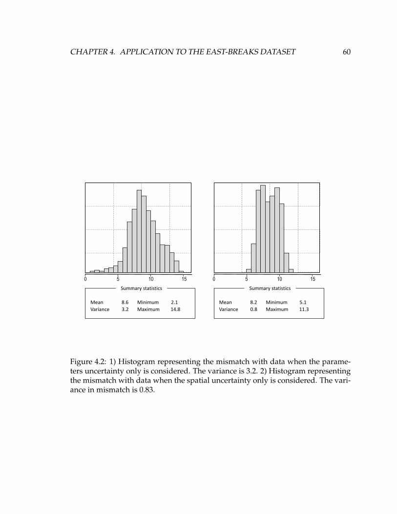
CHAPTER 4. APPLICATION TO THE EAST-BREAKS DATASET 60
0 5 10 15
Summary statistics
Mean 8.6
Variance 3.2
Minimum 2.1
Maximum 14.8
0 5 10 15
Summary statistics
Mean 8.2
Variance 0.8
Minimum 5.1
Maximum 11.3
Figure 4.2: 1) Histogram representing the mismatch with data when the parame-ters uncertainty only is considered. The variance is 3.2. 2) Histogram representingthe mismatch with data when the spatial uncertainty only is considered. The vari-ance in mismatch is 0.83.

CHAPTER 4. APPLICATION TO THE EAST-BREAKS DATASET 61
4.6 Sensitivity analysis
The input parameters considered in the study are presented in Table 2. The same
ranges of variability are used. Our sensitivity analysis is based on 200 realizations.
Only linear interactions between two parameters are considered. We assume that
the other interactions are one order of magnitude less important. Figure 4.3 shows
the importance of each parameter in terms of data-fit through a Pareto plot. The
red line corresponds to the significance level, meaning that the parameter values
that cross the line are statically influential to the model data-fit. The results show
that the Tau parameter, the variance and covariance of the noise are the most influ-
encing parameters in term of data fitting. The Tau parameter is important because
it modifies the probability maps used to draw lobe locations. Therefore, it directly
impacts the lobes stacking patterns. Two reasons explain the importance of the
Gaussian noise. First, perturbing the geometry of the lobes changes the internal
layering of the model. The second reason is related to the shape of the deposition
surfaces. The placement of the lobes is primarily controlled by the topography.
The added noise modifies this topography; thus influencing the placement of the
lobes Figure 4.4.
4.7 Optimization results
4.7.1 Definition of the number of iterations
The Tau value and the Gaussian noises added on top of the lobes are optimized
by using the sequential (step-by-step) optimization. To validate the efficiency of
this approach, one must ensure that the computational time carried out by the
optimization process is not too large. This is even more critical in our case study
since the analysis of the model spatial uncertainty and the parameters sensitivity
already requires considerable CPU time. In the runs performed in the sensitivity
analysis, we observed that the number of lobes in the models varies from 10 to
15. To control the total CPU time, each optimization sequence of the conditioning

CHAPTER 4. APPLICATION TO THE EAST-BREAKS DATASET 62
Figure 4.3: Pareto plot showing the importance of each parameter on the data-fit.

CHAPTER 4. APPLICATION TO THE EAST-BREAKS DATASET 63
Perturbation Perturbation
Lobe n+1Lobe n+1
Lobe nLobe n
Figure 4.4: The lobe n is perturbed with two different noises. The first noise createsa low topography on the right of the lobe. The following lobe logically fills it(left pictures). The second noise creates a low topography on the left of the lobe,generating sedimentation in this location (right pictures). This example shows theimportance of the noise in the placement of the lobes

CHAPTER 4. APPLICATION TO THE EAST-BREAKS DATASET 64
approach is stopped after 50 iterations. The associated computational time for
the full optimization scheme (approximatively 1.5h) is assumed to be reasonable
enough for the method to be integrated in a real modeling workflow. However,
better matches would be obtained with longer optimization runs.
4.7.2 Initial guess
The initial parameter values are randomly drawn from the prior distributions. As
expected, the initial model does not match the data set: the sediment package is
thinner and covers a larger area of the domain (Figure 4.5, Figure 4.7) and the lobes
thicknesses are not reproduced at the well location (Figure 4.6).
4.7.3 Optimized model
The optimized model is composed of 12 lobes and displays the main features
present in the East-Breaks data (Figure 4.5). Most of the deposited lobes are gath-
ered around the proximal part of the basin (near the source), and no deposition
occurs in the distal part. The high and low sedimentation areas are therefore accu-
rately reproduced. The similarity between the thickness maps extracted from the
data and the simulated one confirms the quality of the match. From the error map,
we can see that most of the mismatch is located near the sediment source area. At
this location, the environment of deposition is, in general, high energy, and the as-
sociated erosion process is intense. A source of residual misfit might be the model
of erosion, which is probably not accurate enough.
The simulated lobes compare well with the ones recorded in the log data. How-
ever, the surface-based model produces slightly less variability in terms of lobe
thicknesses (Figure 4.6). This is probably due to the use of lobe thickness proba-
bility distributions that poorly reproduce the actual thickness variability. Another
reason could be the erosion model, which may be too simplistic. High variability
in the recorded thickness can indeed mean high variability in erosion intensities.
Figure 4.7 displays the internal layering of the geological model at different
stages of the optimization process. The initial guess presents a poor match with
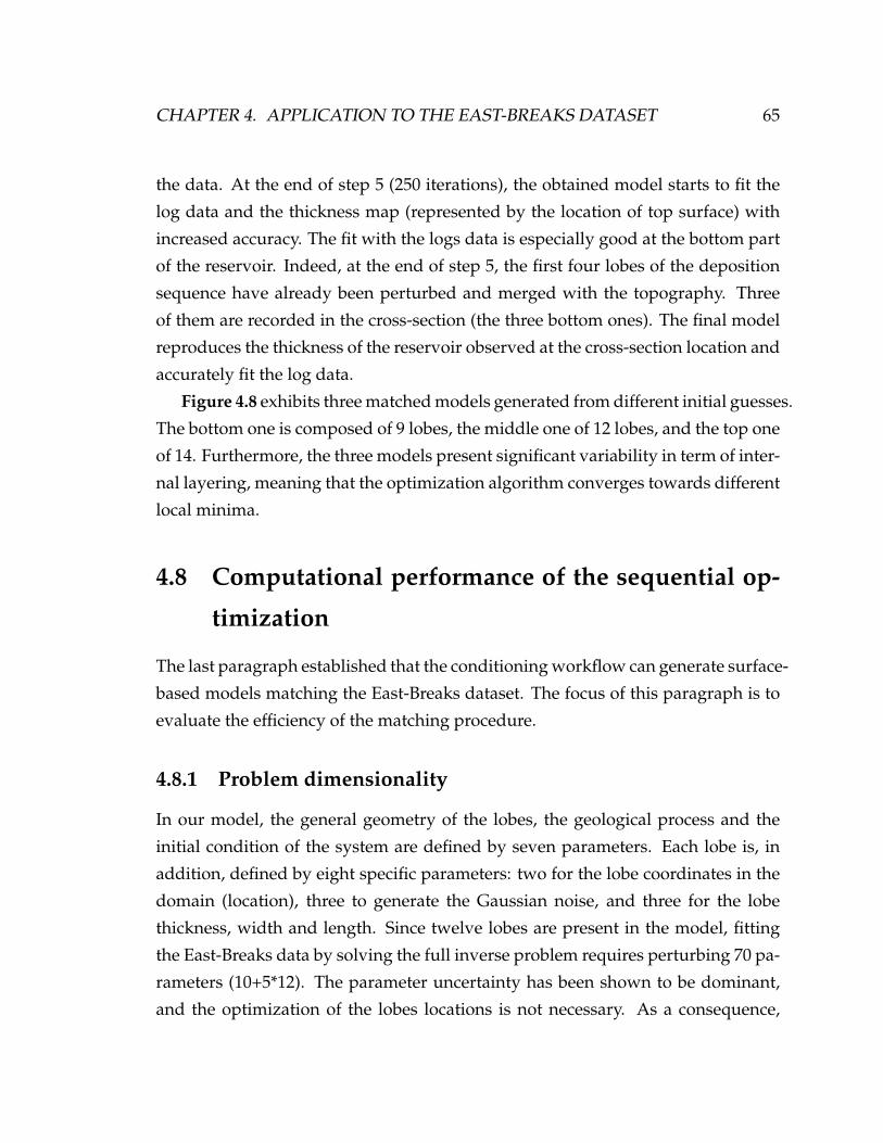
CHAPTER 4. APPLICATION TO THE EAST-BREAKS DATASET 65
the data. At the end of step 5 (250 iterations), the obtained model starts to fit the
log data and the thickness map (represented by the location of top surface) with
increased accuracy. The fit with the logs data is especially good at the bottom part
of the reservoir. Indeed, at the end of step 5, the first four lobes of the deposition
sequence have already been perturbed and merged with the topography. Three
of them are recorded in the cross-section (the three bottom ones). The final model
reproduces the thickness of the reservoir observed at the cross-section location and
accurately fit the log data.
Figure 4.8 exhibits three matched models generated from different initial guesses.
The bottom one is composed of 9 lobes, the middle one of 12 lobes, and the top one
of 14. Furthermore, the three models present significant variability in term of inter-
nal layering, meaning that the optimization algorithm converges towards different
local minima.
4.8 Computational performance of the sequential op-
timization
The last paragraph established that the conditioning workflow can generate surface-
based models matching the East-Breaks dataset. The focus of this paragraph is to
evaluate the efficiency of the matching procedure.
4.8.1 Problem dimensionality
In our model, the general geometry of the lobes, the geological process and the
initial condition of the system are defined by seven parameters. Each lobe is, in
addition, defined by eight specific parameters: two for the lobe coordinates in the
domain (location), three to generate the Gaussian noise, and three for the lobe
thickness, width and length. Since twelve lobes are present in the model, fitting
the East-Breaks data by solving the full inverse problem requires perturbing 70 pa-
rameters (10+5*12). The parameter uncertainty has been shown to be dominant,
and the optimization of the lobes locations is not necessary. As a consequence,
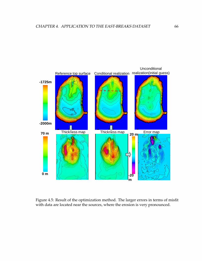
CHAPTER 4. APPLICATION TO THE EAST-BREAKS DATASET 66
-1725m
-2000m
Reference top surface
Unconditional
realization(initial guess)Conditional realization
Thickness map Error mapThickness map70 m
0 m
20 m
-20
m
Figure 4.5: Result of the optimization method. The larger errors in terms of misfitwith data are located near the sources, where the erosion is very pronounced.
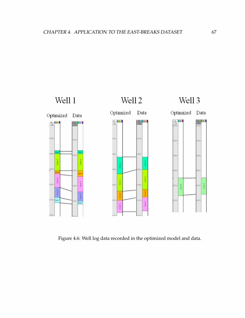
CHAPTER 4. APPLICATION TO THE EAST-BREAKS DATASET 67
Figure 4.6: Well log data recorded in the optimized model and data.

CHAPTER 4. APPLICATION TO THE EAST-BREAKS DATASET 68
Figure 4.7: Cross-section of the model at different steps of the optimization process.Each lobe is represented by a different colored zone.

CHAPTER 4. APPLICATION TO THE EAST-BREAKS DATASET 69
Figure 4.8: Three matching models generated from different initial guesses.
CHAPTER 4. APPLICATION TO THE EAST-BREAKS DATASET 70
the number of parameters to optimize was reduced to 46 (10+3*12). The sensitiv-
ity analysis shows that the Tau parameter and the parameters generating the lobe
noises are the most influential. Retaining only those influential parameters results
in a subset of 37 parameters (1+3*12). By using the developed sequential optimiza-
tion, the problem is then divided into 13 different steps: an initial one to optimize
the Tau value and one for each lobe’s noise optimization. In other words, the initial
70-dimensional problem is handled by solving one 1D optimization problem and
twelve 3D problems.
4.8.2 Benchmark
Several runs are generated using our step-by-step optimization approach. Those
runs start from different initial guesses. Each optimization sequence is set to stop
after 50 model evaluations. The total number of iterations varies therefore from
600 iterations (for 11 lobes) to 800 iterations (for 15 lobes). To evaluate the effi-
ciency of the method, we must first to verify that the generated data-fit is one of
the best fits that the forward model can produce. This requires evaluating what
is a ”good fit.” To address this issue, our approach is compared with a random
sampling approach. The 70 parameters are randomized and 10000 realizations are
generated (performing a larger number of simulations is difficult due to compu-
tational costs). The minimal mismatch is set as a reference. This value gives a
reasonable indication of what a ”good fit” can be. All the 70 parameters (and not
only the most influential 37) are randomized to ensure that the full variability of
the model is captured. We must also evaluate the speed of convergence of the de-
veloped method. The comparison is done with a brute-force approach, where the
37 parameters are optimized simultaneously. The Nelder-Mead method is chosen
as the optimization algorithm. The total number of iterations is also set to 700.

CHAPTER 4. APPLICATION TO THE EAST-BREAKS DATASET 71
4.8.3 Results
Our conditioning workflow achieves a better match than a random sampling of
10000 iterations (Figure 6.6). It also outperforms the brute-force optimization ap-
proach in terms of speed of convergence and quality of fit, which tends to be over-
whelmed by the amount of parameters (37 at once). The mismatch generated by
our method dramatically decreases during the first 100 iterations. These 100 iter-
ations correspond to the two first steps of the optimization scheme. During these
two steps, the depositional model (Tau parameter) and the geometry of the first
lobe are perturbed, inducing large model changes that may create significant im-
provement of data-fit. The efficiency of the method is even more evident when the
evaluation is based on computational time and not on the number of iterations;
650 iterations (12 lobes) of the traditional method take 2.7 hours (2 hrs 42mn). The
computational time of a forward simulation is 14.9 seconds for 12 lobes. With our
conditioning workflow; 650 iterations require 1.38 hours (1 hr 23mn). The aver-
age computational time of a forward simulation is 7.6 seconds in average for 12
lobes. The reason for such improvement is that the simulation time of one forward
model decreases after each optimization sequence. Indeed, the initial lobe of the
sequence is combined with the topography and does not need to be resimulated in
the following steps (3.5). The improvement in computational time of 48% is con-
sistent with the theoretically calculated improvement (2.3). The efficiency of the
method can also be assessed by comparing the computational time necessary to
reach the 0.5 mismatch threshold (considered as a ’good fit’). With brute-force op-
timization, only one run reaches the threshold, in 1.25 hours. With our method, all
the optimization runs reach the threshold, in 0.4 to 0.6 hours (100 to 200 iterations).
4.9 Summary of the chapter
In this chapter, the developed conditioning framework was successfully applied
to a real data set composed of a thickness map and wells data. The first step of
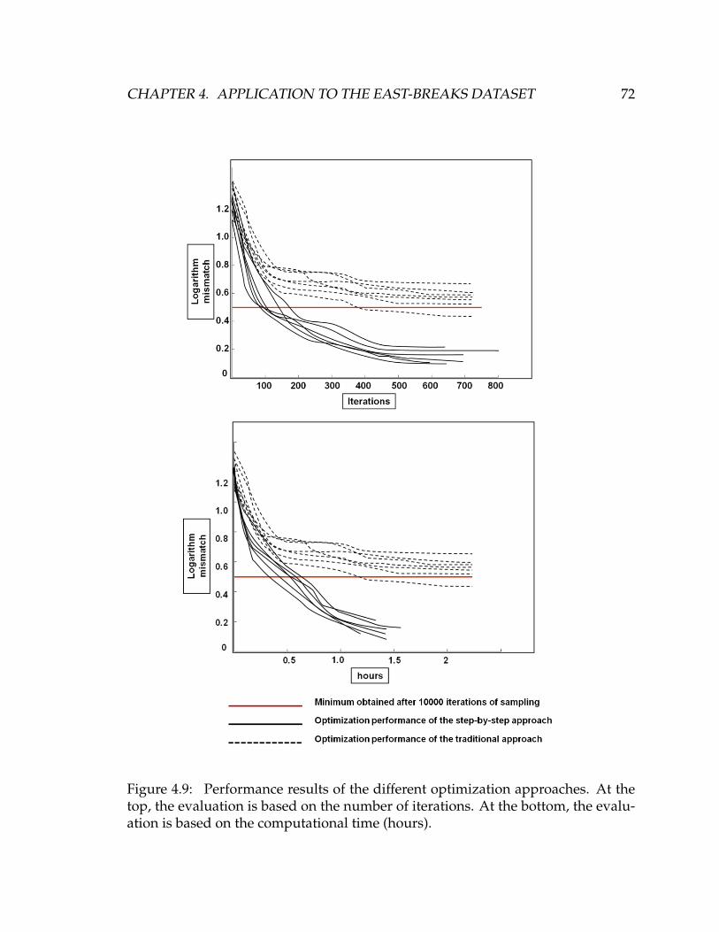
CHAPTER 4. APPLICATION TO THE EAST-BREAKS DATASET 72
Figure 4.9: Performance results of the different optimization approaches. At thetop, the evaluation is based on the number of iterations. At the bottom, the evalu-ation is based on the computational time (hours).

CHAPTER 4. APPLICATION TO THE EAST-BREAKS DATASET 73
the method identified the input parameter uncertainty as the leading one. The
second step, which is the sensitivity analysis of the input parameters, filtered the
Tau parameter (from the depositional model) and the parameters controlling the
noise added on top of each lobe as the most influencing parameters. The sequential
optimization of the remaining parameters achieves an accurate and efficient match
with the data.

Chapter 5
Hierarchical modeling of lobe
structures
5.1 Introduction
In this chapter, the conditioning approach previously presented is used to generate
multi-scales lobes structures, and more precisely lobes and lobe-elements. The key
idea relies on using the conditioning methodology within a hierarchical modeling
workflow. In such workflow, the large scale objects (the lobes) are simulated first.
The smaller lobe-elements are then embedded inside the lobes using our condition-
ing approach. This approach is tested on a real data-set named MS1 (Multi-Scale
1).
5.2 Motivation for hierarchical modeling
Sedimentation processes occur at a vast range of spatial and temporal scales. As
a consequence, several scales of structures are observed inside sediments pack-
ages (Charvin et al., 1995; Garland et al., 1999). For lobe systems, the scales of
these elements vary from meters with sand beds, to tens of kilometers with lobes
complexes (2.2). Two structures are however most likely to impact the reservoir
74

CHAPTER 5. HIERARCHICAL MODELING OF LOBE STRUCTURES 75
flow response: the lobes and lobe-elements. Lobe-elements are elongated sheets
of sand, up to 5 km in length and a few meters thick (Gervais et al., 2006) When
stacked, lobe-elements form a lobe. Lobes and lobe-elements may be bounded by
significant layers of shales, hence controlling reservoir connectivity (Saller et al.,
2008).
In surface-based modeling, a possible approach to reproduce such multi-scale
heterogeneities is to model the multi-scale deposition and erosion processes that
generate such structures. It requires a surface-based model that can mimic differ-
ent scales of sedimentation processes and integrate them all together. For lobes
and lobe-element deposits, a multi-scale model should reproduce two different
processes: one that allows forming a lobe by stacking lobe-elements, and another
one that switches the deposition of lobe-elements to distinct areas of the domain,
such that different lobes are generated.
An alternative idea, commonly employed in geological modeling, is using a
hierarchical modeling approach (Deutsch and Wang, 1996; Li and Caers, 2011).
The lobes (the largest elements) are generated first, with a surface-based model.
The smaller lobes-elements are then simulated (by surface-based modeling), and
embedded inside the previously generated lobes by applying the conditioning ap-
proach. Thus, the final model presents a hierarchy of depositional bodies, with
small stacks of lobe-elements forming lobes. In this chapter, this hierarchical mod-
eling approach is applied to a real data-set that provides information on both lobes
and lobe-elements thicknesses.
Developing a method for modeling multiscale structures in a surface-based
model framework is important because (1) surface-based models are tailored for
turbidite reservoirs, (2) turbidite reservoirs present a hierarchy of structures that
impact flows and (3) one must to rely on an accurate model to generate these struc-
tures because few data are available.
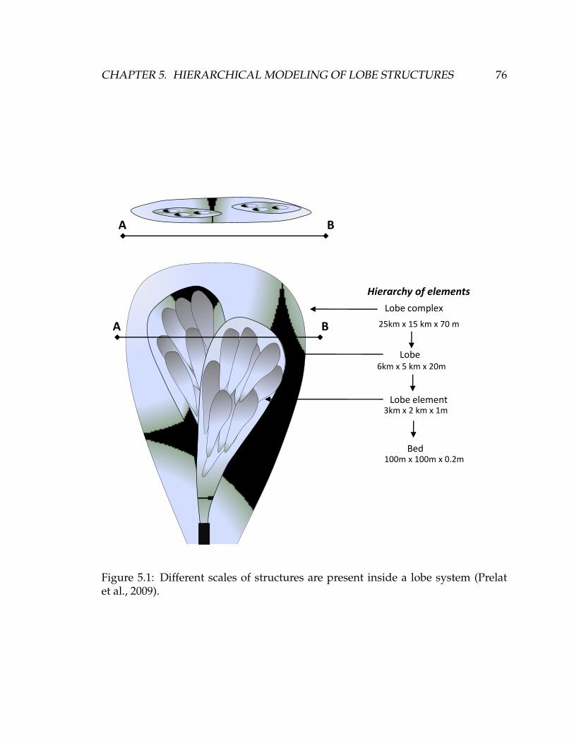
CHAPTER 5. HIERARCHICAL MODELING OF LOBE STRUCTURES 76
A B
A B
Hierarchy of elements
Lobe complex
Lobe
Lobe element
Bed
6km x 5 km x 20m
25km x 15 km x 70 m
3km x 2 km x 1m
100m x 100m x 0.2m
Figure 5.1: Different scales of structures are present inside a lobe system (Prelatet al., 2009).
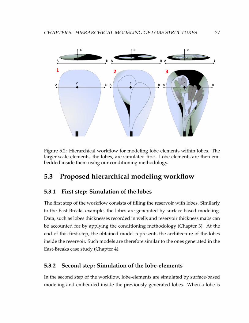
CHAPTER 5. HIERARCHICAL MODELING OF LOBE STRUCTURES 77
A
A B
A
A B
A
A B
B B BC CC
C C C
1 2 3
Figure 5.2: Hierarchical workflow for modeling lobe-elements within lobes. Thelarger-scale elements, the lobes, are simulated first. Lobe-elements are then em-bedded inside them using our conditioning methodology.
5.3 Proposed hierarchical modeling workflow
5.3.1 First step: Simulation of the lobes
The first step of the workflow consists of filling the reservoir with lobes. Similarly
to the East-Breaks example, the lobes are generated by surface-based modeling.
Data, such as lobes thicknesses recorded in wells and reservoir thickness maps can
be accounted for by applying the conditioning methodology (Chapter 3). At the
end of this first step, the obtained model represents the architecture of the lobes
inside the reservoir. Such models are therefore similar to the ones generated in the
East-Breaks case study (Chapter 4).
5.3.2 Second step: Simulation of the lobe-elements
In the second step of the workflow, lobe-elements are simulated by surface-based
modeling and embedded inside the previously generated lobes. When a lobe is

CHAPTER 5. HIERARCHICAL MODELING OF LOBE STRUCTURES 78
filled with lobe-elements, these lobe-elements are deposited from lobe bottom to
top. The forward simulation stops when the volume of deposited lobe-elements
equals the lobe volume. Our conditioning approach is used to optimize the lobe-
elements location and shape such that the thickness of the generated deposit matches
the lobe thickness (i-e shape). Well-data informing on the lobe-elements thick-
nesses can also be accounted for when applying the conditioning methodology.
Therefore, filling each lobe requires the solution of an optimization problem.
At the end of this second step, the final model is a set of surfaces representing
(1) the lobes geometries and, inside each lobe, (2) the lobe-elements. The multi-
scale structures are therefore reproduced.
5.4 Application to the MS1 dataset
5.4.1 The MS1 data
The hierarchical modeling workflow is tested on a real data-set , called MS1 (Multi-
Scale 1) and composed of four wells, a top and a bottom surface. The reservoir is
18 km wide by 30 km long (Figure 5.3) and filled with turbidite lobes. Since the
geological system has not be deformed by tectonics, no structural restoration is re-
quired. The bottom surface is used directly as the deposition surface on which the
geobodies are stacked. The thickness map of the sediments is then computed from
the top surface. The wells record individual thicknesses for both lobes and lobe-
elements (Figure 5.4). The two surfaces and the log measurements are interpreted
from raw data and are therefore uncertain. Usually, uncertainty is handled by em-
ploying different alternatives datasets. In our study, MS1 is considered to be one of
these alternatives datasets. The following MS1 example is similar to many early-
development studies of turbidite reservoirs, with few available data and possibly
different scales of heterogeneities impacting the flow (R.Slatt and Weimer, 1999).

CHAPTER 5. HIERARCHICAL MODELING OF LOBE STRUCTURES 79
Well 1
Well 2
Well 3
Well 4
Bottom surface Top surface
Figure 5.3: Top and bottom surfaces of the MS1 reservoir.
5.4.2 Lobe modeling
Input parameters
The lobes are simulated using the surface-based model presented in Chapter 2.
Sedimentation and erosion processes are specified by seven parameters (5.1). In
addition, each deposited lobe is defined by eight specific parameters: three pa-
rameters for the lobe shape (width, length, thickness), two parameters for the lobe
locations, and three parameters for the Gaussian noise generation. Since these
parameters are uncertain, they are represented by probability distributions. Un-
fortunately, the MS1 data do not provide enough information to accurately infer
these distributions.
To address this issue, an analog of the reservoir is generated by process-based
modeling (Tao Sun and Hongmei Li, personal communications). The MS1 bottom
surface is used as an initial topography on which the sediments deposition is sim-
ulated. The initial conditions of the process-based model, such as average grain
size, input flow and sediments discharge are defined to be representative of tur-
bidite lobe systems (Miller et al., 2008). Although the process-based simulation
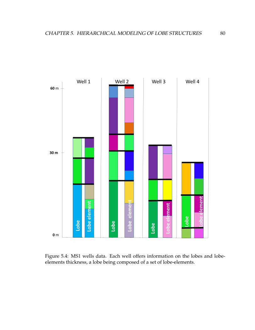
CHAPTER 5. HIERARCHICAL MODELING OF LOBE STRUCTURES 80
Well 1 Well 2 Well 3 Well 4Lo
be
Lob
e e
lem
en
t
Lob
e
Lob
e e
lem
en
t
Lob
e
Lob
e e
lem
en
t
0 m
60 m
30 m
Lob
e
Lob
e e
lem
ent
Figure 5.4: MS1 wells data. Each well offers information on the lobes and lobe-elements thickness, a lobe being composed of a set of lobe-elements.

CHAPTER 5. HIERARCHICAL MODELING OF LOBE STRUCTURES 81
result is not conditioned to the MS1 data, its geological realism provides informa-
tion on the general deposition patterns (Figure 5.5), information that can be used
to define the parameters probability distributions. However, inferring such statis-
tics is difficult because it implies delineating different geobodies in a continuous
sequence of sediments, with no clear boundaries between objects. For instance, it
necessiates identifying the thin layer of shale bounding the lobes and then extract-
ing the associated geobodies characteristics. Since the shale layers present some
areas of non-deposition or erosion and are not continuous, their designation is te-
dious (Michael et al., 2010). The difficulty of extracting lobe geometries precisely
leads to a large variability in the inferred probability distributions.
Another issue to consider when interpreting a process-based model is that the
locations and intensity of erosion that occurs during the simulation are not re-
tained. Extracting the original lobes thicknesses before erosion is therefore not
possible. Instead, the statistics are defined so that the generated surface-based sim-
ulations display thicknesses after erosion similar to those present in the process-
based model. The stopping criterion for a simulation is the volume of deposited
sediments, the target volume being defined by the MS1 thickness map. The ob-
tained probability distributions are presented in table 5.1.
Definition of the objective function
In the MS1 case-study, generating a conditional model means reproducing a spe-
cific thickness map and wells measurements. The nature of the data to match in
the MS1 and East-Breaks case studies is therefore similar (4.4). As a consequence,
the same objective function is used.
Weighting spatial uncertainty versus parameter uncertainty
When conditioning the MS1 data, the first step of the methodology is to evalu-
ate which of the two uncertainties (parameter or spatial) impacts the data-fit. To
this end, two sets of 200 realizations are generated: one with constant input pa-
rameters, and varying spatial parameters and the other one with varying input

CHAPTER 5. HIERARCHICAL MODELING OF LOBE STRUCTURES 82
Parameters Distribution
Lobe
element
Geometry
Width Uniform [500m 2000m]
Length Uniform [1000m 4000m]
Thickness Uniform [2m 10m]
Variance of the noise Uniform [0 x]
x depending on the maximum lobe thickness
Covariance of the noise Uniform [500m 4000m]
Geological
process
Progradation intensity Uniform [300m 800m]
Migration intensity Uniform [200m 700m]
Tau value Uniform [0 1]
Parameters Distribution
Lobe
Geometry
Width Uniform [2000m 5000m]
Length Uniform [3000m 6000m]
Thickness Uniform [5m 35m]
Variance of the noise Uniform [0 x]
x depending on the maximum lobe thickness
Covariance of the noise Uniform [1000m 6000m]
Geological
process
Progradation intensity Uniform [1000m 2000m]
Migration intensity Uniform [600m 1200m]
Tau value Uniform [0 1]
Table 5.1: Input parameters required to run a forward simulation and their asso-ciated distributions.
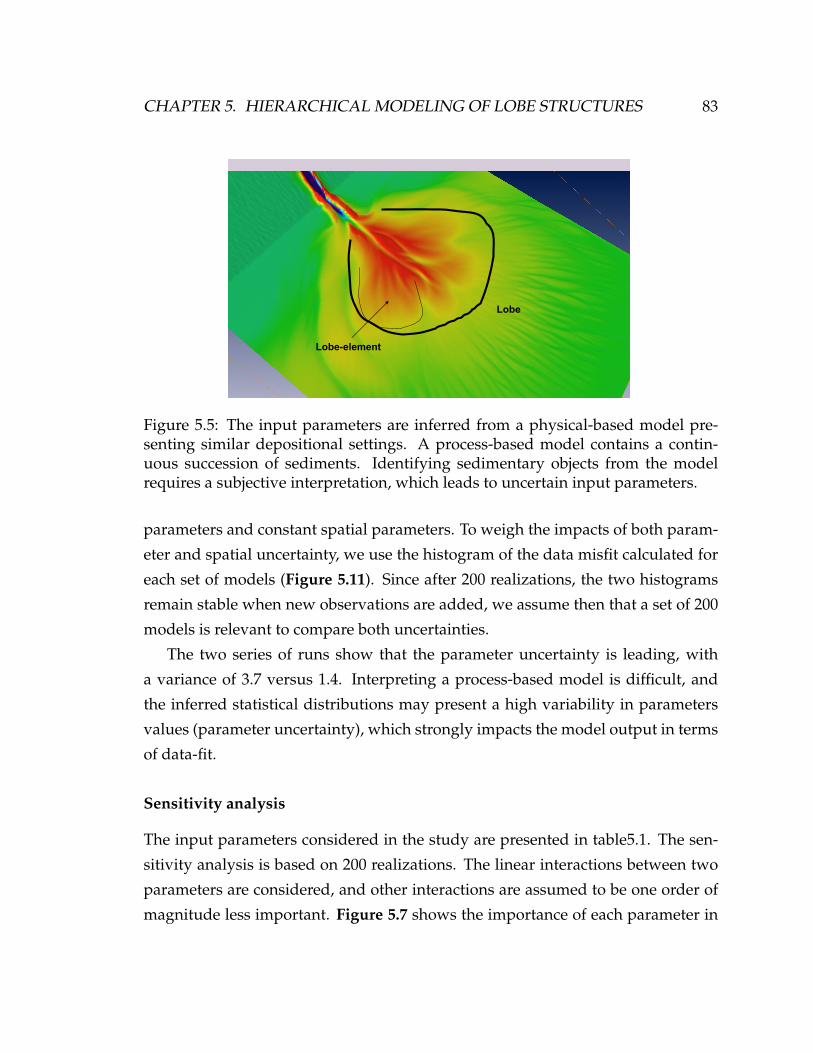
CHAPTER 5. HIERARCHICAL MODELING OF LOBE STRUCTURES 83
Lobe-element
Lobe
Figure 5.5: The input parameters are inferred from a physical-based model pre-senting similar depositional settings. A process-based model contains a contin-uous succession of sediments. Identifying sedimentary objects from the modelrequires a subjective interpretation, which leads to uncertain input parameters.
parameters and constant spatial parameters. To weigh the impacts of both param-
eter and spatial uncertainty, we use the histogram of the data misfit calculated for
each set of models (Figure 5.11). Since after 200 realizations, the two histograms
remain stable when new observations are added, we assume then that a set of 200
models is relevant to compare both uncertainties.
The two series of runs show that the parameter uncertainty is leading, with
a variance of 3.7 versus 1.4. Interpreting a process-based model is difficult, and
the inferred statistical distributions may present a high variability in parameters
values (parameter uncertainty), which strongly impacts the model output in terms
of data-fit.
Sensitivity analysis
The input parameters considered in the study are presented in table5.1. The sen-
sitivity analysis is based on 200 realizations. The linear interactions between two
parameters are considered, and other interactions are assumed to be one order of
magnitude less important. Figure 5.7 shows the importance of each parameter in

CHAPTER 5. HIERARCHICAL MODELING OF LOBE STRUCTURES 84
200
180 1
500
Figure 5.6: 1) Histogram representing the mismatch with data when only the pa-rameter uncertainty is considered. The variance is 3.7. 2) Histogram representingthe mismatch with data when only the spatial uncertainty is considered. The vari-ance in mismatch is 1.4.

CHAPTER 5. HIERARCHICAL MODELING OF LOBE STRUCTURES 85
4 6 8 10 12 14 16
1
2
3
4
5
6
7
8
9
10Tau
Variance
Covariance
Migration:progradation
Length
Width: Length
Thickness
Progradation
Tau:variance
Migration
Figure 5.7: Pareto plot showing the importance of each parameter on the data-fit.
terms of data-fit through a Pareto plot. The results show that the Tau parameter
controlling the model of deposition, the lobe thickness, the variance and covari-
ance of the noise are the most influencing parameters in term of data-fit. The be-
havior of the model is globally similar to the one observed in the East-Breaks case
study, which is logical because the data and the simulated geobodies are of the
same nature.
Optimization and resulting conditioned model
In this step, the parameters identified as influential are optimized sequentially. The
first sequence consists of optimizing the Tau value controlling the model of depo-
sition (general parameters). In the following sequences, starting from the bottom
lobe, the parameters controlling the thickness and Gaussian noise are optimized
(lobe-specific parameters). One should ensure that the computational time carried

CHAPTER 5. HIERARCHICAL MODELING OF LOBE STRUCTURES 86
out by the optimization process is not too high since another series of optimiza-
tions is also needed to fill the lobes with lobe-elements. As a consequence, each
optimization step is set to stop after 200 model evaluations. The matched model
is composed of 6 lobes generated after 1200 iterations (6*200) or two hours. When
compared to the well data, the simulated model accurately fits the recorded struc-
tures (Figure 5.9). All the lobes are deposited in the north part of the domain, and
the sediments thickness matches the MS1 thickness map (Figure 5.8). From the
error map, we can see that most of the mismatch is located near the channel car-
rying the sediments to the system (Figure 5.8). Indeed, the surface-based model
is tailored to reproduce the deposition associated with unconfined sediments flow
typical of lobe systems. The model is however not able to reproduce structures
generated by a confined flow of sediments within a channel. It would indeed re-
quire different sedimentation and erosion models.
5.4.3 Lobe-elements modeling
In the previous step of the workflow, the reservoir was filled with lobes. In or-
der to reproduce the multi-scale structures, these lobes must now be filled with
lobe-elements. For each lobe, the lobe elements are deposited on the lobe bottom
surface. In order to precisely embed the lobe-elements inside the lobe, the lobe
thickness map is used as a constraint, and the lobe-elements are placed using the
optimization approach. Filling the 6 lobes generated in the previous step means
solving 6 optimizations problems. Each optimization problem is handled in the
same way the lobe conditioning is handled: evaluation of the leading uncertainty,
analysis of sensitivity, and reformulation of the optimization problem.
Regarding geological characteristics, lobe-elements present similar shapes and
stacking patterns compared with lobes 2.3.1, but on a smaller scale. It is indeed
common in sedimentology that small-scale structures mimic the spatial organiza-
tion of larger ones (Stow and King, 2000; Wagoner et al., 2003). Such behavior can
be observed in the process-based model (Figure 5.5).
Because of these geological similarities between lobes and lobe-elements, the
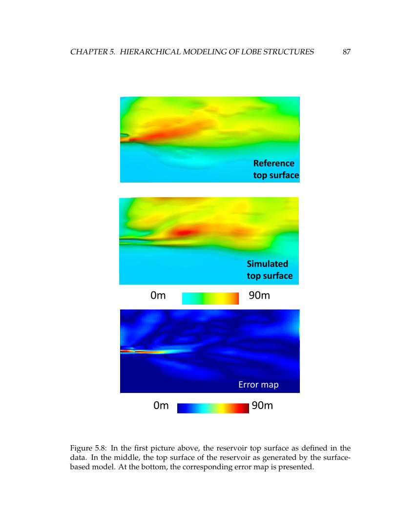
CHAPTER 5. HIERARCHICAL MODELING OF LOBE STRUCTURES 87
10
20
30
40
50
60
70
80
90
100
102030405060708090100
10 20 30 40 50 60 70 80
0m
Reference top surface
Simulated top surface
Error map
90m
0m 90m
Figure 5.8: In the first picture above, the reservoir top surface as defined in thedata. In the middle, the top surface of the reservoir as generated by the surface-based model. At the bottom, the corresponding error map is presented.

CHAPTER 5. HIERARCHICAL MODELING OF LOBE STRUCTURES 88
w1 w1
w2 w2
w3 w3
w4 w4
Figure 5.9: The internal layering of the reservoir at the lobe-element scale.

CHAPTER 5. HIERARCHICAL MODELING OF LOBE STRUCTURES 89
surface-based model that has been used for lobes simulation is also used for the
lobe-elements; the input parameters values describe , however, smaller-scale pro-
cesses: smaller geobodies sizes, smaller migration and progradation ranges, smaller
erosion intensity, etc.
Specification of the input parameters
The parameters required to simulate lobe-elements deposition are uncertain and
should be represented with probability distributions. The lobe-elements thick-
nesses recorded in the four wells are, however, not informative enough to prop-
erly infer such statistics. Instead, the probability distributions are inferred from
the same process-based model that has been used to determine lobes characteris-
tics (Figure 5.5). In the first step of the workflow, the process-based model was
divided into lobes. For each lobe, it is now possible to identify the embedded
lobe-elements. It consists on finding the bounding layers of shale and any changes
in grain-sizes. The obtained probability distributions are presented in 5.1. Such
interpretation is possible because process-based models simulate sedimentation
processes at the grain -size level, thus generating the different scales of structures
present in the reservoir.
Definition of the objective function
Since the generated lobe-elements should also reproduce a thickness map and the
well measurements, the objective function used in this step is similar to the previ-
ously used.
Weighting spatial uncertainty
When constraining lobe-elements inside lobes, the first step of the methodology is
to evaluate which of uncertainty -parameter or spatial- is leading. This step should
be performed for each of the six lobes filling, because each filling is a different
optimization problem. However, in order to speed up the process, the evaluation is
performed only for the filling of the bottom lobe. We assume then that the obtained
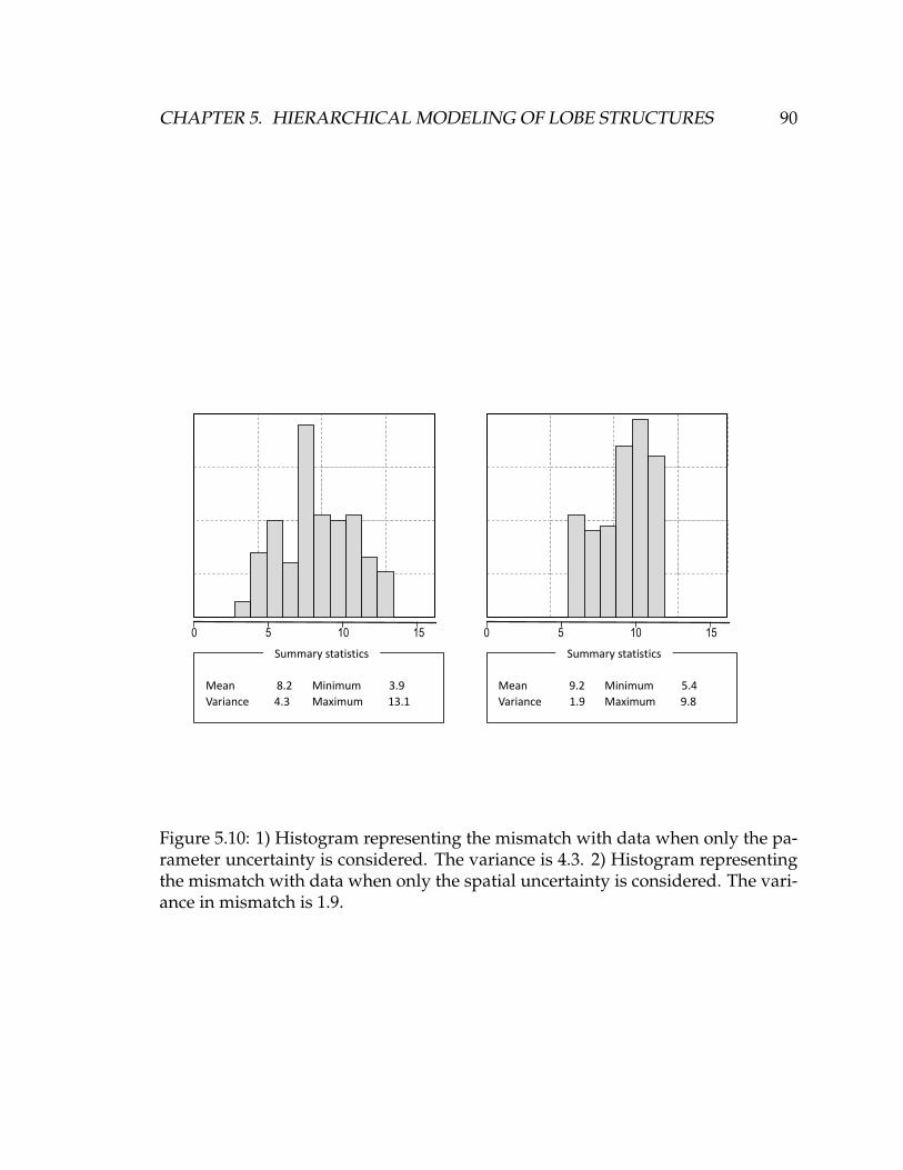
CHAPTER 5. HIERARCHICAL MODELING OF LOBE STRUCTURES 90
0 5 10 15
Summary statistics
Mean 8.2
Variance 4.3
Minimum 3.9
Maximum 13.1
0 5 10 15
Summary statistics
Mean 9.2
Variance 1.9
Minimum 5.4
Maximum 9.8
Figure 5.10: 1) Histogram representing the mismatch with data when only the pa-rameter uncertainty is considered. The variance is 4.3. 2) Histogram representingthe mismatch with data when only the spatial uncertainty is considered. The vari-ance in mismatch is 1.9.
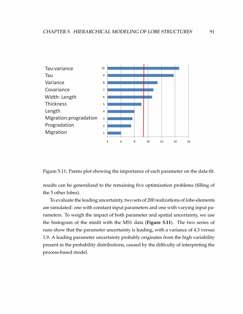
CHAPTER 5. HIERARCHICAL MODELING OF LOBE STRUCTURES 91
4 6 8 10 12 14 16
1
2
3
4
5
6
7
8
9
10
Tau
Variance
Covariance
Migration:progradation
Length
Width: LengthThickness
Progradation
Tau:variance
Migration
Figure 5.11: Pareto plot showing the importance of each parameter on the data-fit.
results can be generalized to the remaining five optimization problems (filling of
the 5 other lobes).
To evaluate the leading uncertainty, two sets of 200 realizations of lobe-elements
are simulated: one with constant input parameters and one with varying input pa-
rameters. To weigh the impact of both parameter and spatial uncertainty, we use
the histogram of the misfit with the MS1 data (Figure 5.11). The two series of
runs show that the parameter uncertainty is leading, with a variance of 4.3 versus
1.9. A leading parameter uncertainty probably originates from the high variability
present in the probability distributions, caused by the difficulty of interpreting the
process-based model.

CHAPTER 5. HIERARCHICAL MODELING OF LOBE STRUCTURES 92
Sensitivity analysis
The second step, when constraining the lobe-elements inside a lobe, is to perform a
sensitivity analysis of the input parameters. This step should be repeated six times,
once for each lobe being filled. However, this may incur high computational costs.
To avoid this issue, the sensitivity analysis is performed only on the filling of the
first lobe, and the results are generalized to all the lobes. Our sensitivity analysis
is based on 200 realizations. The input parameters considered in the study are
presented in Table 5.1, and the same ranges of variability are used.
The result of the sensitivity analysis (Figure 5.7) shows that the Tau parame-
ter, the lobe width, length, the variance and covariance of the noise are the most
influential parameters in terms of data fitting.
Resulting model
In this step, the six conditioning problems are solved by optimizing the most in-
fluential parameters. For each conditioning problem (each lobe being filled), the
optimization is divided into sequences. The first sequence optimizes the Tau value
(general parameter) and the following sequences, one for each lobe-element, opti-
mize the geobodies noise, width and length.
The final surface-based model is composed of 6 lobes and 37 lobe-elements,
with an average of five lobe-elements per lobe. Since the lobe-elements are placed
inside the lobes, the natural hierarchy observed in sedimentary systems is modeled
(Figure 5.13 and Figure 5.14). The average computation time required to embed
the lobe-elements inside a single lobe is 1 hour.
Since the lobes match the thickness map and well measurements and the gen-
erated lobe-elements fit the thicknesses measured in the four wells Figure 5.12, the
final model is therefore a conditional multi-scale surface-based model. It is gen-
erated in less than 8 hours (Matlab code): 2 hours for the lobe simulations and
6 hours for the lobe-elements modeling (6*1 hour). The relatively high computa-
tional cost is caused by the complexity of the data-set.
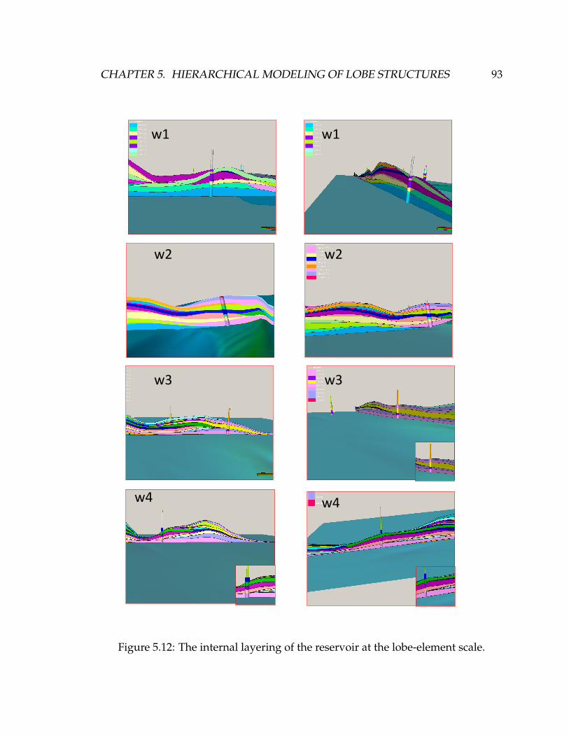
CHAPTER 5. HIERARCHICAL MODELING OF LOBE STRUCTURES 93
w1 w1
w2 w2
w3 w3
w4 w4
Figure 5.12: The internal layering of the reservoir at the lobe-element scale.

CHAPTER 5. HIERARCHICAL MODELING OF LOBE STRUCTURES 94
a b
Figure 5.13: A) Top surface of the lobe simulated with the surface-based model.B) Top surface of the stack of lobe-elements embedded in the lobe. The matchbetween the two structures is very strong. The higher roughness of the surface Bis caused by the stacking of distinct geobodies.
5.5 Summary of the chapter
In the previous chapter, lobes were simulated and matched to real reservoir data:
a realistic representation of the lobes structure inside the reservoir was generated.
Yet, representing the lobes may be insufficient to model realistically the flow re-
sponse of the reservoir. Indeed, different scales of structures typically control the
connectivity of turbidite reservoirs (Li and Caers, 2011). Consequently, in this
chapter, a new application of the conditioning workflow is proposed to gener-
ate multi-scale structures. The key idea of the method is to simulate the largest
elements first and to constrain the smaller ones by applying our developed condi-
tioning workflow. The method has been successfully tested on the real and com-
plex MS1 data-set.

CHAPTER 5. HIERARCHICAL MODELING OF LOBE STRUCTURES 95
a
b
Figure 5.14: A) Bottom and top surfaces of lobe B) Internal layering of lobe-elements inside a lobe.

Chapter 6
Conditioning by means of hybrid
optimization
6.1 Introduction
The key goal of the presented conditioning method is to decrease the dimension-
ality of the optimization problem. For this purpose, three methods have been pro-
posed: an assessment of the leading uncertainty, a sensitivity analysis, and a re-
formulation of the optimization problem. The two previous examples, East-Breaks
and MS1, provide a context in which the parameter uncertainty is dominant and
few parameters are identified as leading, significantly simplifying the optimization
problem. In this chapter, the conditioning approach is improved to handle cases
where sensitivity analysis and uncertainty assessment do not lead to model sim-
plifications. The improved algorithm is tested on a real data set originated from
the Karoo Basin.
6.2 Problem statement
Once the optimization problem has been divided into sequences, a critical step
is selecting the algorithm used to solve each optimization sequence. Since the
96
CHAPTER 6. CONDITIONING BY MEANS OF HYBRID OPTIMIZATION 97
model does not respond continuously to small variations in the input parame-
ters, a derivative-free optimization is required. In order to be efficient, the selected
method must also be able to identify efficiently within the search space the promis-
ing regions that can lead to matching models. This step is called exploration or
global search. Once one of these regions has been identified, the method must then
be able to converge rapidly to a local minimum. This step is called exploitation
or local search. Our conditioning workflow has been successfully applied using
the Nelder-Mead (NM) simplex method, an optimization algorithm more tailored
for exploitation than exploration (Nelder & Mead, 1965). In the case studies, the
models were constrained to a thickness map and logs data. The sensitivity anal-
ysis identified the noise added on top of each lobe and the Tau value controlling
the model of deposition as the most influential parameters in term of data-fit. As a
consequence, decreasing the number of parameters to optimize is possible, leading
to an important reduction of the search-space size. Its exploration is therefore rela-
tively easy, which explains the strong performance of the Nelder-Mead algorithm.
However, reducing the number of parameters may not always be possible. Indeed,
the spatial uncertainty can be too influential to obtain meaningful sensitivity anal-
ysis results. In such a case, the search space (at each sequence of optimization) is
very large. Threrefore, it becomes critical to develop an optimization algorithm
that is robust in term of exploration and exploitation.
6.3 Optimization background
Optimization approaches called global are very good by nature at performing ex-
ploration (Horst et al., 2000). They are, however, not efficient when it comes to ex-
ploitation. On the contrary, local search techniques (such Nelder-Mead) are good
at exploitation but not efficient for exploration. These complementary strengths in-
spired the development of the hybrid approach. Hybrid algorithms employ global
search methods for exploration and local search techniques for exploitation, and
they perform better than the individual algorithms independently. This research
explores the possibility of improving the Nelder-Mead algorithm by hybridizing it

CHAPTER 6. CONDITIONING BY MEANS OF HYBRID OPTIMIZATION 98
with the Genetic Algorithm, a global search approach.
6.3.1 Hybrid approach
Genetic Algorithm (GA) is a robust global search method based on analogies to
biology and genetics (Goldeberg, 1989). Survival of the best among a population
of individuals, selection criteria, and reproduction strategies is a concept copied
from natural life. The search algorithm starts from an initial population of param-
eters realizations and performs the following cycle of operations until a stopping
criterion is reached.
Two important features need to be assessed in order to develop a hybrid scheme
between GA and NM. The first one is to define when to switch between global
optimization and local optimization when searching for a solution. The adopted
approach is applying the genetic algorithm to a population of individuals first.
The best solution among the optimized population is further improved using the
Nelder-Mead algorithm (Figure 6.1). The number of function evaluations per-
formed by each algorithm is defined as input. The second feature to investigate
is the creation of the initial simplex used by the Nelder-Mead approach. The local
search is indeed extremely sensitive to the shape of the simplex because it gives
information about the landscape of the function being optimized. In this work, we
choose to construct the simplex using the closest individuals from the best one in
terms of parameter values (within the optimized population of individuals). The
hybrid algorithm is applied for each sequence of optimization.
Algorithm 6.3.1 Hybrid Optimization Algorithm1) Randomly initialize a population of individuals.2) Perform the Genetic Algorithm optimization for n iterations or t seconds.3) Identify the best individual.4) Construct the simplex with the best individual and the nd closest individuals ( nddimension of the problem).5) Perform the Nelder-Mead optimization for n iterations or t seconds.
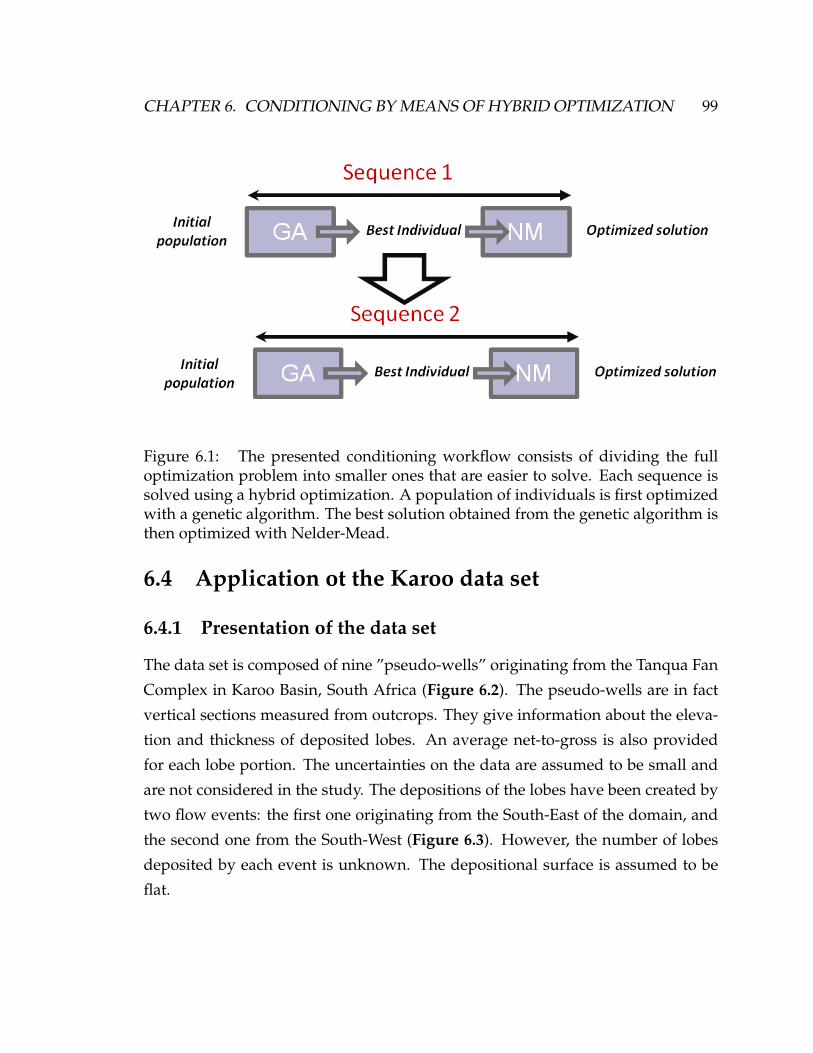
CHAPTER 6. CONDITIONING BY MEANS OF HYBRID OPTIMIZATION 99
Figure 6.1: The presented conditioning workflow consists of dividing the fulloptimization problem into smaller ones that are easier to solve. Each sequence issolved using a hybrid optimization. A population of individuals is first optimizedwith a genetic algorithm. The best solution obtained from the genetic algorithm isthen optimized with Nelder-Mead.
6.4 Application ot the Karoo data set
6.4.1 Presentation of the data set
The data set is composed of nine ”pseudo-wells” originating from the Tanqua Fan
Complex in Karoo Basin, South Africa (Figure 6.2). The pseudo-wells are in fact
vertical sections measured from outcrops. They give information about the eleva-
tion and thickness of deposited lobes. An average net-to-gross is also provided
for each lobe portion. The uncertainties on the data are assumed to be small and
are not considered in the study. The depositions of the lobes have been created by
two flow events: the first one originating from the South-East of the domain, and
the second one from the South-West (Figure 6.3). However, the number of lobes
deposited by each event is unknown. The depositional surface is assumed to be
flat.
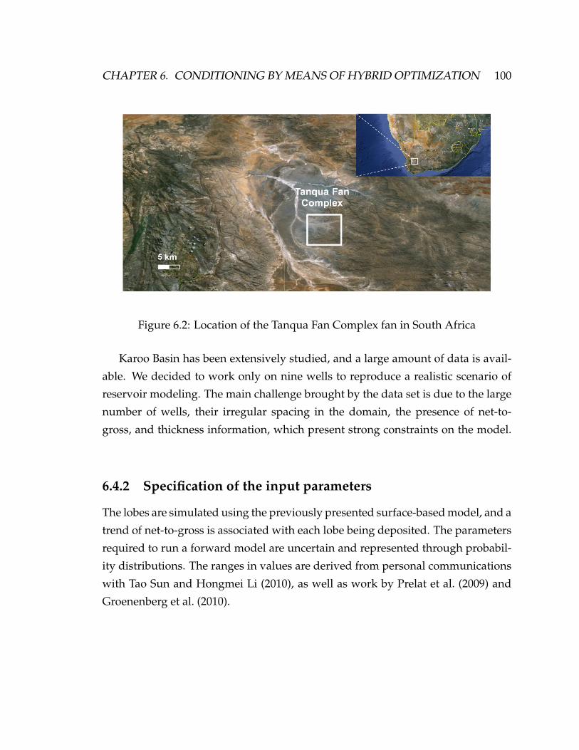
CHAPTER 6. CONDITIONING BY MEANS OF HYBRID OPTIMIZATION 100
Figure 6.2: Location of the Tanqua Fan Complex fan in South Africa
Karoo Basin has been extensively studied, and a large amount of data is avail-
able. We decided to work only on nine wells to reproduce a realistic scenario of
reservoir modeling. The main challenge brought by the data set is due to the large
number of wells, their irregular spacing in the domain, the presence of net-to-
gross, and thickness information, which present strong constraints on the model.
6.4.2 Specification of the input parameters
The lobes are simulated using the previously presented surface-based model, and a
trend of net-to-gross is associated with each lobe being deposited. The parameters
required to run a forward model are uncertain and represented through probabil-
ity distributions. The ranges in values are derived from personal communications
with Tao Sun and Hongmei Li (2010), as well as work by Prelat et al. (2009) and
Groenenberg et al. (2010).

CHAPTER 6. CONDITIONING BY MEANS OF HYBRID OPTIMIZATION 101
Figure 6.3: Locations of the wells in the domain. Two flow events originating fromthe South-East and the South-West of the domain created the observed structures.The sources of sediments are not exactly known, but they are assumed to be locatedinside the two windows.

CHAPTER 6. CONDITIONING BY MEANS OF HYBRID OPTIMIZATION 102
Parameters Distribution
Lobe
Geometry
Width Uniform [2000m 4000m]
Length Uniform [5000m 10000m]
Thickness Uniform [5m 20m]
Variance of the noise Uniform [0 4]
Covariance of the noise Uniform [1000m 6000m]
Geological
process
Progradation intensity Uniform [500m 1000m]
Migration intensity Uniform [200m 700m]
Tau value Uniform [0 1]
Number of lobes source 1 Uniform [0-10]
Number of lobes source 2 Uniform [0-10]
Initial
condition
Coordinates X Y of the
sediments source 1
Unique and uniformly distributed in a window of
4km by 4km situated at the right of the domain ().
Flow direction source 1
Uniform [-40 0]
Coordinates X Y of the
sediments source 2
Unique and uniformly distributed in a window of
4km by 4km situated at the left of the domain
Flow direction source 2
Uniform [0 40]
Table 6.1: Input parameters required to run a forward simulation and their asso-ciated distributions.

CHAPTER 6. CONDITIONING BY MEANS OF HYBRID OPTIMIZATION 103
6.4.3 Objective function
In the case study, a matched model should fit, for each well, the recorded lobe
thickness and net-to-gross. The mismatch at a single well location is computed as
follows:
Ewelli = Ethickness + ENTG (6.1)
Ethickness is the value of the mismatch in terms of lobe thicknesses :
Ethickness =1
NLobesdata
NLobesdata
∑1
|Thick data lobei− Thick simulated lobei|Thick data lobei
(6.2)
E(ntg) is the penalty created by the mismatch in net-to-gross, defined as
Entg =1
NLobesdata
NLobesdata
∑1
|NTG data lobei− NTG simulated lobei|NTG data lobei
(6.3)
The final objective function is then computed as follows:
Etotal =9
∑1
Ewelli (6.4)
6.4.4 Results of the sensitivity analysis
Two sets of model realizations (200 realizations each) are generated, one with con-
stant input parameters and one with varying input parameters. As a criterion, we
use the histogram of the data misfit calculated for each set of models.
As a result, we observe that spatial uncertainty and parameter uncertainty have
similar impacts on the model output (Figure 6.4). This means that once a set of
input parameters values have been selected, the final choice in the lobe location
strongly impacts the data-fit. In this situation, identifying the most influential in-
put parameters with a sensitivity analysis is challenging because the relationship

CHAPTER 6. CONDITIONING BY MEANS OF HYBRID OPTIMIZATION 104
0 4 8 12
Summary statistics
Mean 7.7
Variance 2.5
Minimum 1.7
Maximum 11.9
0 4 8 12
Summary statistics
Mean 7.5
Variance 2.6
Minimum 1.1
Maximum 12.3
Figure 6.4: On the right, the histogram representing the mismatch with data whenonly the parameters uncertainty is considered. The variance is 2.5. On the left, thehistogram representing the mismatch with data when only the spatial uncertaintyis considered. The variance in mismatch is 2.6

CHAPTER 6. CONDITIONING BY MEANS OF HYBRID OPTIMIZATION 105
Figure 6.5: Pareto plot showing the importance of each parameter or combinationof parameters on the data-fit. None of the parameters statistically impact the modelresponse (the level of significance is not reached). One of the possible reasons is thespatial stochasticity that can alter the sensitivity analysis results, making it difficultto identify the leading parameters.
input parameters/output is altered by the spatial stochasticity of the model. When
performing a sensitivity analysis (Figure 6.5), the results show that none of the pa-
rameters or parameter combinations has been identified as having a statistically
significant effect on the model output; they do not reach the level of significance
(level of significance p=0.01; Scheidt and Caers (2009). In order to achieve a match
with the data, all the input parameters and lobe locations must therefore be opti-
mized; the model cannot be simplified.
CHAPTER 6. CONDITIONING BY MEANS OF HYBRID OPTIMIZATION 106
6.4.5 Optimization performance
The first sequence of optimization perturbs the general parameters. General means
that the values of these parameters are randomly selected before starting the simu-
lation, and they don’t need to be redrawn during the process. The Tau parameter,
migration and progradation intensity, location and flow orientations of the sources,
numbers of deposited lobes belong to this family. The total number of parameters
to optimize in this sequence is then 11. The following optimization sequences fo-
cus on optimizing the lobe-specific parameters. Lobe-specific means that the value
of these parameters must be randomly drawn for each lobe being deposited: lo-
cation, width, length and thickness of the lobe, as well as the Gaussian noise pa-
rameters. For each of these sequences, the total number of parameters to optimize
was 8. The initial population used by the Genetic Algorithm is composed of 20
individuals. We assume this number is a good compromise between computation-
ally efficiency and population diversity. We should also notice that the efficiency
of Genetic Algorithm is greatly dependent on its tuning parameters (probability of
mutation and crossover, population size, (Goldeberg, 1989). However, the purpose
of this work is not to evaluate how the tuning parameters impact the efficiency of
the approach. As a consequence, all the optimization runs are generated using the
default values defined in Matlab (2009). For each sequence, the total number of
forward simulations (function evaluations) is set to 500. This includes the evalua-
tions performed by the Genetic Algorithm and the Nelder-Mead Algorithm. Since
each forward simulation lasts for 3 seconds, 500 iterations can be executed in 25
minutes. The proportion of function evaluations performed respectively by the
Genetic Algorithm and the Nelder-Mead method can be specified before starting
an optimization run. GA80%NM20% (Figure 6.6) means 400 function evaluations
have been performed by the Genetic Algorithm (20 generations of GA) and 100
by the Nelder-Mead approach. Different runs are performed with hybridization
ratios varying from 100% (pure global optimization using exclusively the GA) to
0% (pure local optimization using exclusively NM). This approach allows for the

CHAPTER 6. CONDITIONING BY MEANS OF HYBRID OPTIMIZATION 107
identification of which method or hybrid scheme is best suited to obtain an accu-
rate match.
6.4.6 Results
The results indicate that the Nelder-Mead approach achieves the worst match (Fig-
ure 6.6). Hybrid schemes with a relatively high ratio of global optimization (com-
pared to local optimization) perform the best. Those results stress the importance
of exploration for finding solutions to the optimization problem. The poor perfor-
mance of Nelder-Mead alone can indeed originate from the algorithm having con-
verged to a local minimum and failed at exploring the search space for better solu-
tions. It should also be noticed that global optimization is not sufficient to generate
accurate matching models. A step of local search is also required. The best results
are indeed observed for GA70%NM30%, GA60%NM40% and GA50%NM50%. A
ratio of global optimization higher than 70% tends to reduce the quality of the
match. Performing all the runs and identifying the best hybridization ratio is time-
consuming tasks. However, we observe that the first hundred iterations are al-
ready informative about the ratio efficiency. Hence, an efficient ratio can be se-
lected before the optimizations are carried to the end.
The surface-based model generated with the GA70%NM30% hybrid scheme
is presented in Figure 6.7. Ten lobes have been deposited, five originating from
the first source and five from the second one (Figure 6.8). The model presents a
complex internal layering caused by the amalgamation of the lobes (Figure 6.7).
The average sediments thickness is 20 meters. At the wells locations (Figure 6.9),
the number of lobes simulated by the forward model always matches the number
observed in the data. In terms of lobe thicknesses, the produced mismatch is, on
average, 0.42 meter per lobe. Since the average lobe thickness measured in the
data is 9.5 meters, the misfit is less than 5% of the total lobe thickness. Figure 6.11
shows that the variability of the mismatch is slightly higher for thicker lobes. It
originates from the definition of the objective function; the function computes a
relative error between the real thickness observed in the wells and the simulated
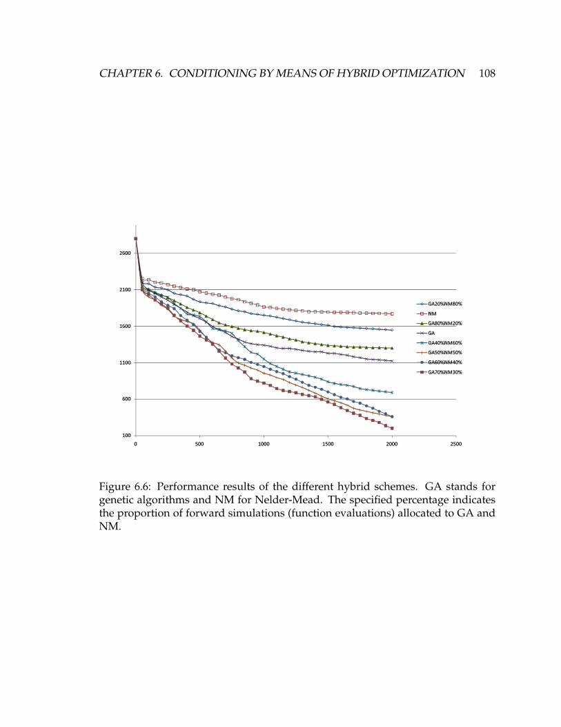
CHAPTER 6. CONDITIONING BY MEANS OF HYBRID OPTIMIZATION 108
Figure 6.6: Performance results of the different hybrid schemes. GA stands forgenetic algorithms and NM for Nelder-Mead. The specified percentage indicatesthe proportion of forward simulations (function evaluations) allocated to GA andNM.

CHAPTER 6. CONDITIONING BY MEANS OF HYBRID OPTIMIZATION 109
one. One percent error for a thick lobe means a larger mismatch in thickness units
than 1% error for a thin lobe.
In terms of net-to-gross, the match is not as good. The average misfit is 0.12
for an average net-to-gross of 0.43 (27% of error). Figure 6.11 shows that the mis-
match is more pronounced for low net-to-gross (shale) measurements. Such errors
can be observed in wells 3, 2 and 8, where thick shale sections are not reproduced
by the model (Figure 6.7). The conceptual net-to-gross trend limits the shale de-
posits to the extremities of the lobe, where lobe thickness tends to be the thinnest.
The model therefore cannot produce thick deposits of shale similar to the ones
observed in the data. This means that our conceptual model on radial decrease
in thickness and net-to-gross is too simplistic (it does not account for small-scale
heterogeneities) or that the quantity of shale in the lobes is underestimated.
The model generated with the Nelder-Mead approach alone is presented in
Figure 6.10. The accuracy of the data-fit is not as good. First, the number of lobes
simulated by the surface-based model in wells 3 and 9 does not match the number
observed in the data. Secondly, the produced mismatch is, on average, 1.7 meters
per lobe, (20%). In term of net-to-gross, the average misfit is 0.23 (50 % error).
From Figure 6.10, we observe again the model’s difficulty with producing thick
shale deposits (wells 1, 2, 4 and 8). We also notice that the quality of the fit is very
different from one well to another. A good match in terms of thickness and net-to-
gross is achieved for wells 4 and 5, whereas wells 3 and 9 are not matched at all.
The fact that some wells are accurately fitted while others are totally mismatched
confirms that the Nelder-Mead algorithm is trapped in a local minimum. Indeed,
in this example, obtaining a better match would require modifying the sequence
of optimization so that more sedimentation occurs at the location of wells 3 and
9. This calls for large updates in the model, hence exploring new regions of the
search space. The Nelder-Mead is not able to perform this global search. Instead,
the algorithm improves the fit by locally searchings new solutions, creating small
perturbations in the model and improving the fit only for some of the wells. This
shows the importance of using a hybrid approach because it performs a robust ex-
ploration of the search space, avoids being trapped in a local minimum, and can

CHAPTER 6. CONDITIONING BY MEANS OF HYBRID OPTIMIZATION 110
Figure 6.7: Model generated by the hybrid optimization approach. A) Initial depo-sitional surface. B) Top surface of the sediments package. C) Lateral section of themodel. D) Longitudinal section of the model.
also perform smaller updates in the models to achieve a precise match with the
data. Using a hybrid optimization approach would have been therefore prefer-
able in the East-Breaks and MS1 case-studies, even though good results have been
obtained with Nelder-Mead
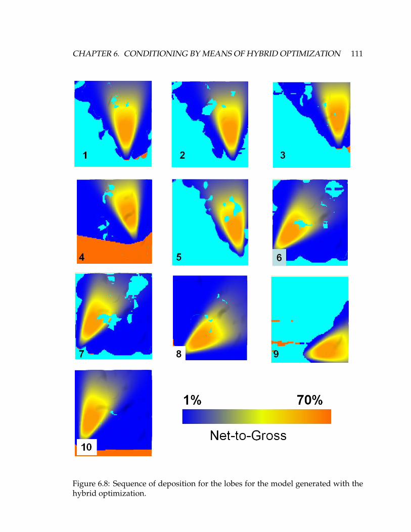
CHAPTER 6. CONDITIONING BY MEANS OF HYBRID OPTIMIZATION 111
Figure 6.8: Sequence of deposition for the lobes for the model generated with thehybrid optimization.
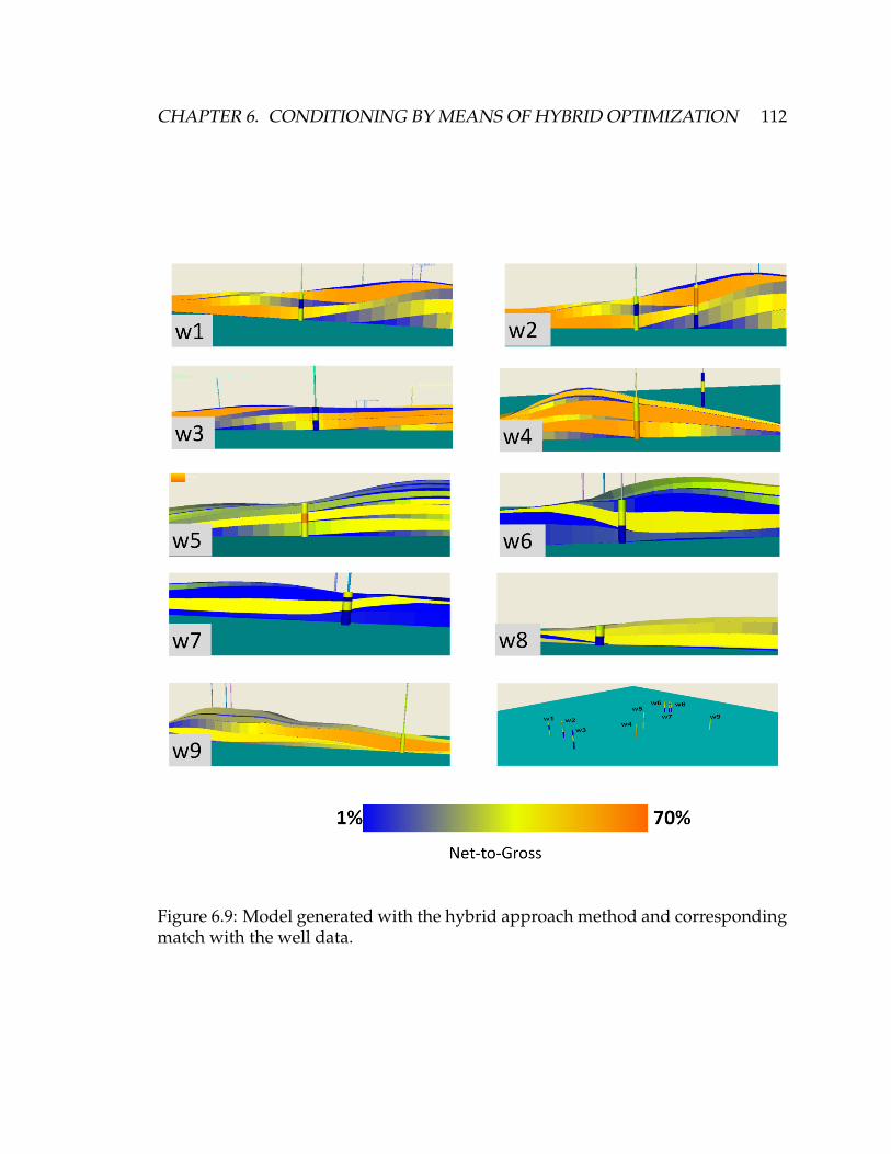
CHAPTER 6. CONDITIONING BY MEANS OF HYBRID OPTIMIZATION 112
Figure 6.9: Model generated with the hybrid approach method and correspondingmatch with the well data.
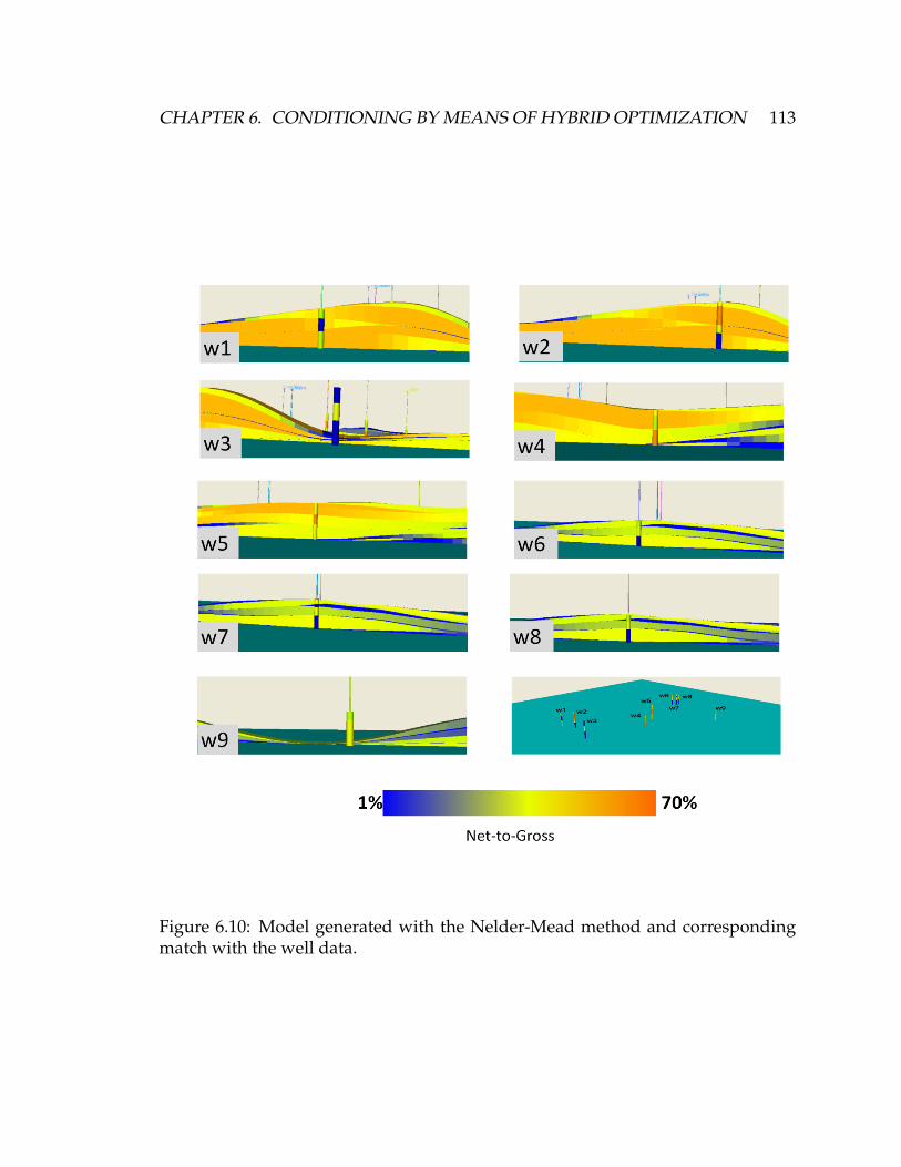
CHAPTER 6. CONDITIONING BY MEANS OF HYBRID OPTIMIZATION 113
Figure 6.10: Model generated with the Nelder-Mead method and correspondingmatch with the well data.

CHAPTER 6. CONDITIONING BY MEANS OF HYBRID OPTIMIZATION 114
Figure 6.11: Left: Cross-plot between measured lobe thicknesses in the data andthe mismatches of the model after a hybrid optimization. Right: Cross-plot be-tween measured net-to-gross in the data and mismatches of the model after a hy-brid optimization.
6.5 Models prediction accuracy
6.5.1 Purpose of fitting models to data
The aim of reservoir modeling is to predict the reservoir structures where data
are not available or not informative enough. The obtained model is then used to
make decisions about the field development and management. The underlying
assumption behind reservoir modeling is that, by matching the available data, the
prediction accuracy of the model is improved. The model integrates specific in-
formation about the reservoir. However, any prediction is uncertain. The model
is an approximation of reality, the data contains various types of errors and may
be insufficient to constrain a single model, and the model parameters values may
not be precisely known. Decisions therefore should be based on a population of
models that accounts for this uncertainty and not just on a single model.
To study how the prediction performances are improved by data-conditioning,
a cross-validation based on the Karoo dataset is performed. Well 9 is first removed
from the data (Figure 6.12). One hundred models are then generated and con-
strained to the eight remaining wells. At the well 9 location, the simulated struc-
tures are extracted and compared to the real ones. This test enables one to evaluate
CHAPTER 6. CONDITIONING BY MEANS OF HYBRID OPTIMIZATION 115
how accurate a population of models is in terms of prediction. Well 9 has been
chosen because it is located away from the other data, hence it is more difficult to
predict. The case-study can then be regarded as a real exploration scenario where
the structures at well 9 have to be forecasted for future drilling. Correctly predict-
ing the geological structures in such a case is critical because, first, one wants to
reach a reservoir layer and not drill a dry well, and secondly, an optimized well
path may be developed from the generated model. Any difference between the
model and the real reservoir structures may lead to additional drilling costs.
6.5.2 Cross-validation results
The prediction of optimizations runs are evaluated at five different computational-
times (0, 1, 3, 6, and 9 hours), meaning five different levels of accuracy of fit to the
data. Figure 6.12 displays these results. For each computational time, a bar repre-
senting the spread between best and worst match and best and worst prediction of
the generated models is plotted.
We see logically that the longer the computational time (more iterations), the
better the data-fit is. However, when plotting computational time versus predic-
tions accuracy, the obtained trend is different. The accuracy increases for the first
six hours; the variability between models is reduced due to data constraints, and
these models tend to better predict the structure of well 9 because they integrate
the information present in the data. After six hours, however, the predictive ac-
curacy worsens; additional optimization iterations increase the model mismatch
with the real well 9 structures.
Different reasons can explain such trends. First, the data present errors. The
models are constrained to erroneous information, so the forecasts are incorrect too.
In the Karoo study, we assumed that data errors are minimal since a precise obser-
vation of the outcrop (from where the data are extracted) is possible. Nonetheless,
mistakes in interpretations may still exist.
The second problem can originate from the surface-based model itself. Because
CHAPTER 6. CONDITIONING BY MEANS OF HYBRID OPTIMIZATION 116
the model simplifies reality, it may not be able to reproduce the geological com-
plexity observed in the data. Perfectly matching the eight wells does not guarantee
that the structures at well 9 will be correctly forecasted.
The third problem can be caused by the way matched models are generated.
Indeed, errors in model predictions are partially caused by uncertainty surround-
ing the input parameters. For example, we don’t know the exact locations of the
sediments sources or the true thickness of the lobes. To correctly account for such
uncertainty, an exhaustive sampling of the model parameters must be completed.
However, sampling approaches are CPU-costly and optimization techniques are
generally preferred. When a population of matched models is generated by op-
timization, initial guesses are randomly selected such that different areas of the
search space can be explored. However, such approach does not guarantee that
all the possible matching models have been considered; the algorithms may fa-
vor some particular combinations of parameters, generating only models that look
alike. Other matching models that have better predictive abilities are ignored.
6.5.3 Comparison between optimization and rejection sampling
To verify wether the optimization approach alters the predictive abilities of the
generated models, two sets of matched models are compared. The first set is gen-
erated using our optimization approach. The second set is produced by a rejection
sampling algorithm (von Neumann, 1951) .
Rejection sampling
In rejection sampling, a pool of matching models is generated by randomly sam-
pling the parameters distributions. Once a model is generated, its probability to
be accepted in the pool depends on the quality of the data-fit. The function defin-
ing the quality of the fit, from a mismatch value defined by the objective function,
is called likelihood. In our case, the likelihood is a half-Gaussian function (Fig-
ure 6.14). Its expected value is 0 and its variance ranges from 0.007 and 6. A low
variance (small spread of the function) means that the sampling algorithm is very
CHAPTER 6. CONDITIONING BY MEANS OF HYBRID OPTIMIZATION 117
selective and accepts only models with small misfit; a slight mismatch indicates
significant chances of rejecting the model.
Since the rejection-sampling approach is based on a brute-force sampling of the
original distributions, it allows modeling accurately the variability in the models
predictions caused by the parameter uncertainty. A difference between rejection-
sampling and optimization results means therefore that the optimization approach
creates an artificially low variability between generated models, providing an in-
correct model of uncertainty.
Results of the comparison
50000 models are initially simulated (simulating a larger number of model would
have incurred a prohibitive CPU-cost). From this initial population, populations
of matching models are created using different likelihoods. For each population,
the best and worst predictions are plotted (Figure 6.15).
From the previous optimization runs, five sets of matched models have also
been generated (0, 1, 3, 6 and 9 hours). The best and worst predictions of each
optimized population are added to the graph (Figure 6.15). The horizontal coordi-
nate of each line is chosen so that, at this particular location, the average mismatch
of the population generated by optimization is similar to the average mismatch of
the population generated by rejection sampling. This allows for the comparison of
the predictive performance of two populations having the same average data-fit.
From the graph, we see that the prediction accuracy of models generated with
the rejection algorithm improves when the variance of the likelihood decreases
from 6 to 0.06. Information provided by the dataset are integrated in the model,
leading to better predictions. However, predictive accuracy worsens when the
variance is less than 0.06. This can be due to some geological inaccuracy in the
model or errors in the data. For a likelihood variance superior to 0.02, populations
generated by optimization and rejection sampling present similar prediction accu-
racy. It means that the optimization approach is consistent with rejection sampling
in term of uncertainty modeling. For a likelihood variance of 0.02 however, the

CHAPTER 6. CONDITIONING BY MEANS OF HYBRID OPTIMIZATION 118
equivalent population generated by optimization (9 hours) presents worse predic-
tions and lower variability between models. To explain this difference, a problem
to consider is the number of models in each population. A higher number may
indeed mean more variability in predictions. However, in our example, the pop-
ulation generated via optimization (low prediction variability) is composed of 100
models, whereas the population generated via sampling (high prediction variabil-
ity) is composed of 49 models. This means that the optimization approach may
create models that tend to look alike, and that are not representative of all the ex-
isting conditioning models.
Bias introduced by the optimization approach
A visual examination of the optimized models shows that the bottom lobes tend
to be larger than the top lobes (Figure 6.17). For the 100 generated models, the
volume of each lobe is computed (Figure 6.16). The figure shows the average vol-
ume of a lobe according to its place in the deposition sequence (1 being the initial
one). It appears clearly that the bottom lobes are larger than the top ones. When
the same calculus is performed on the model generated by the sampling approach,
such trend does not exist. The conditioning approach tends to create models with
artificially larger lobes at the bottom and small ones at the top. The bias originates
from the reformulation of the optimization problem. Indeed, the bottom lobe is op-
timized first, then the second one, etc. Initially updating larger bottom lobes pro-
duces important changes in the model, which allows for significant improvement
in the data-fit. Such behavior does not occur with small bottoms lobes because
their modifications slightly change the models, hence the data-fit. At the end of
the series of optimization, only models with large bottom lobes are simulated, and
the generated populations present a low variability.
Conclusion of cross-validation
This specific example shows how using an optimization versus sampling approach
can lead to bias in uncertainty modeling. It produces a set of models that look
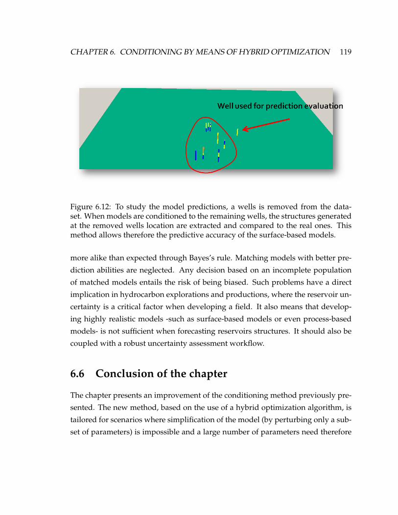
CHAPTER 6. CONDITIONING BY MEANS OF HYBRID OPTIMIZATION 119
Figure 6.12: To study the model predictions, a wells is removed from the data-set. When models are conditioned to the remaining wells, the structures generatedat the removed wells location are extracted and compared to the real ones. Thismethod allows therefore the predictive accuracy of the surface-based models.
more alike than expected through Bayes’s rule. Matching models with better pre-
diction abilities are neglected. Any decision based on an incomplete population
of matched models entails the risk of being biased. Such problems have a direct
implication in hydrocarbon explorations and productions, where the reservoir un-
certainty is a critical factor when developing a field. It also means that develop-
ing highly realistic models -such as surface-based models or even process-based
models- is not sufficient when forecasting reservoirs structures. It should also be
coupled with a robust uncertainty assessment workflow.
6.6 Conclusion of the chapter
The chapter presents an improvement of the conditioning method previously pre-
sented. The new method, based on the use of a hybrid optimization algorithm, is
tailored for scenarios where simplification of the model (by perturbing only a sub-
set of parameters) is impossible and a large number of parameters need therefore

CHAPTER 6. CONDITIONING BY MEANS OF HYBRID OPTIMIZATION 120
Figure 6.13: On top: cross-plot between computational time and data-fit accuracy.Bars represent the spread from worst to best data-fit given a computational time.At bottom: cross-plot between computational time and model predictions. Barsrepresent the spread from worst to best prediction given a computational time.

CHAPTER 6. CONDITIONING BY MEANS OF HYBRID OPTIMIZATION 121
reject
accept
reject
accept
Variance of the gaussian likelihood functions
σ> σ
Likelihood
Figure 6.14: Example of two gaussian likelihood functions. A low variance meansthat the rejection algorithm is very selective and accepts only models with smallmisfit.

CHAPTER 6. CONDITIONING BY MEANS OF HYBRID OPTIMIZATION 122
Figure 6.15: Comparison between predictions generated with the optimizationmethod and a rejection sampling algorithm. For the optimization, the predictionsare calculated with increasing computational time (hence increasing matching ac-curacy). For the rejection sampling, the predictions are computed with increasinglikelihood selectivity (increasing matching accuracy as well). The location of thered bar is chosen so that, at this location, the average data-fit of the populationgenerated by optimization and by sampling are similar.
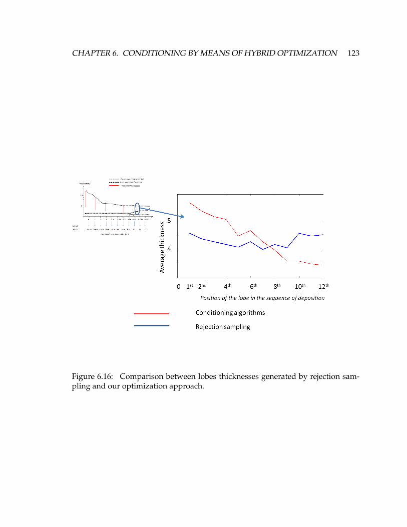
CHAPTER 6. CONDITIONING BY MEANS OF HYBRID OPTIMIZATION 123
Figure 6.16: Comparison between lobes thicknesses generated by rejection sam-pling and our optimization approach.
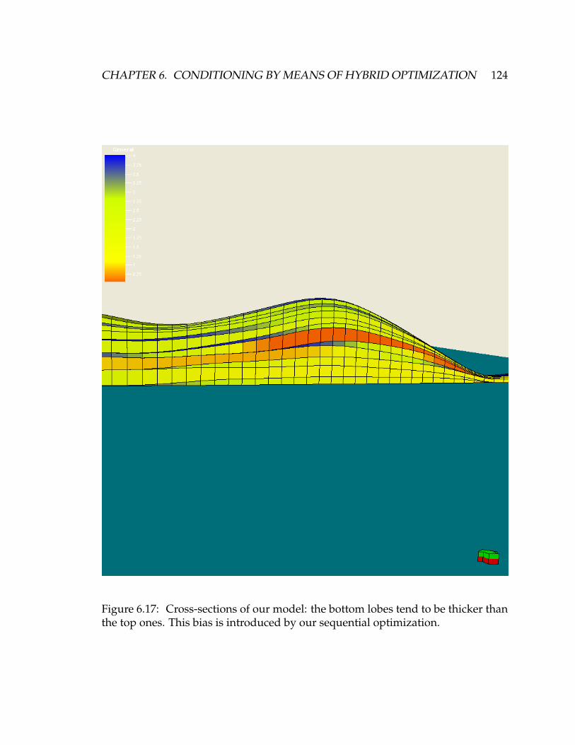
CHAPTER 6. CONDITIONING BY MEANS OF HYBRID OPTIMIZATION 124
Figure 6.17: Cross-sections of our model: the bottom lobes tend to be thicker thanthe top ones. This bias is introduced by our sequential optimization.

CHAPTER 6. CONDITIONING BY MEANS OF HYBRID OPTIMIZATION 125
to be optimized. The method is applied to real vertical measurements from the Ka-
roo Basin. Hybridization shows significant improvement compared to the original
approach. The models achieve an accurate fit with the data in terms of lobe thick-
ness as well as net-to-gross. Most of the residual mismatch originates from the
incapability of the forward model to generate thick sections of shale similar to the
one recorded in the data. The second part shows the drawbacks of optimization in
terms of model predictions. When evaluated on a real-data set, the optimization
approach produces significant biases in predictions. The generated models present
artificially low variability between themselves. This is a critical problem because
the case study proposed in this work can be seen as a real drilling exploration
scenario and with important financial risks at stake.

Chapter 7
Conclusion and Future work
7.1 Conclusion
In this study, we have presented a workflow that allows conditioning surface-
based models to data. Since solving such conditioning problems through optimiza-
tion is CPU-expensive, the key idea behind the proposed workflow is to decrease
the dimensionality of the problem. To this end, three complementary approaches
are developed. The first approach identifies the leading uncertainty. The second
approach is a sensitivity analysis of the input parameters. The third one is a re-
formulation of the optimization problem in order to solve it sequentially and not
simultaneously. This reformulation, by decreasing the number of lobes to simu-
late after each optimization sequence, also reduces the cost of running the forward
model; it is the most novel aspect of the conditioning workflow.
The approach is general in fashion. It can be applied to any data and envi-
ronments of deposition. However, for illustrative purposes, our work focuses on
lobe deposits and static data (more precisely, thickness map and wells). Three real
dataset have been used to evaluate the method’s efficiency and applicability.
The first data-set, named East-Breaks, is composed of a thickness map and three
wells. The case study showed that, first, the conditioning method was able to fit
surface-based models to the data and, secondly, the reformulation of the optimiza-
tion problem was an efficient way to solve the conditioning problem.
126

CHAPTER 7. CONCLUSION AND FUTURE WORK 127
The second data-set named MS1, also composed of a thickness map and well
data, presents the particularity of having two scales of heterogeneity recorded in
the logs. As a consequence, a hierarchical modeling workflow is combined with
our conditioning methodology to generate multi-scale structures. The lobes are
simulated first, and the smaller lobe-elements are then constrained within them
using our conditioning technique.
The third data-set, originating from the Karoo Basin in South Africa, is exclu-
sively composed of wells. It provides a context in which sensitivity analysis and
uncertainty assessment don’t lead to a simplification of the conditioning problem.
To handle the large number of parameters to optimize, a hybrid optimization algo-
rithm is developed. The hybridization scheme presents significant improvements
in speed of convergence. The Karoo dataset provides an opportunity to test the
prediction accuracy of models generated by optimization. From this study, we
conclude that the conditioning methodology is tailored to find efficiently match-
ing models, but is not adequate for uncertainty modeling.
7.2 Future work
The development of surface-based models being relatively recent, tremendous amount
of research is still required to overcome some current limitations. The following
paragraph presents new research ideas classified in three categories: improve-
ments of the surface-based model, improvements of the conditioning methodol-
ogy, and research needs for developing a history-matching workflow. The ideas
are motivated by problems encountered while applying the method to the real
case studies.
7.2.1 Improvement of the surface-based model
Development of a more realistic model
Even though surface-based models generate realistic reservoir structures, the struc-
tures remain a simplification of the actual ones. As a consequence, the model may

CHAPTER 7. CONCLUSION AND FUTURE WORK 128
not be able to reproduce the structure complexity observed in the data. The misfits
observed in the three case studies give insights on the model limitations (in term
of geological realism) and on which features to improve.
• East-Breaks: This case study shows some issues with regards to erosion mod-
eling. In the real structure, the region near the sediments source was shaped
by intense erosion, creating channels-like features that are observable in the
thickness map. However, the surface-based model cannot recreate those
structures because the erosion rules we use are only based on morphologic
features: slope, curvature of the depositional surface, etc. The morphologic
features do affect the erosion, but work in conjunction with the sediments
flow. Hence, an approach based on a dynamic representation of the physical
process is required to produce realistic erosion patterns. Xu (Xu and Mukerji,
2011), for example, is developing a method based on the diffusion equation
to model the erosion process.
• MS1: We have seen in the MS1 case study, that the surface-based model
generates heterogeneities one scale at a time. As a consequence, modeling
multi-scale structures requires the use of a hierarchical modeling workflow,
a time-consuming approach since it requires solving mutiple conditioning
problems. In order to generate multi-scale structures in a forward manner,
deposition and erosion rules should be extended to include a broader ranges
of sedimentary processes that are appropriate for each scale. An example
would be deposition rules that switch the sedimentation to different areas to
the domain, so that distinct lobes can be created from stacking lobe-elements.
• Karoo: A problem encountered in the Karoo case study is reproducing thick
layers of shales. Indeed, our model assumes that shales (low net-to-gross) are
deposited only at the extremity of the lobe, where the lobe thickness is min-
imum. Only thin layer of shales can therefore be generated. However, thick
sections of shale are present in the data. To overcome this problem, two solu-
tions are possible. The first one is increasing the quantity of shales presents in
the lobe. The actual net-to-gross trend is defined between 70% to 1% , which

CHAPTER 7. CONCLUSION AND FUTURE WORK 129
corresponds to 30% to 99% of shales. An updated one would be, for example,
to define the net-to-gross from 50% to 1% (50% to 99% of shale). The second
solutions is to add a stochastic component to the net-to-gross trend so that
the shales deposits are not only confined to the thin extremity of the lobe.
Yet another solution would be to consider the smaller-scale heterogeneities.
Lobe and lobe-elements are generated, and the petrophysical modeling is ap-
plied to the lobe-elements. At the well locations, the mismatch is computed
by averaging the lobe-elements net-to-gross along the vertical section and
comparing it with the data value (which is already the vertical average).
Integration to a structural restoration framework
Surface-based models generate structures as they exist in modern sedimentary sys-
tems. Before hosting hydrocarbons, the sedimentary structures are buried, faulted,
folded and compacted due to tectonic constraints. In order to reproduce a real
reservoir geometry, the deformations that have modified the initial geometry should
also be considered. Restoration methods provides a framework to address this is-
sue (Cobbold, 1978; Durand-Riard et al., 2010). Restoring means that the structural
constraints on the reservoir are relaxed; the sedimentary structures are restored to
their initial geometry. By doing so, a direct link is established between the sedi-
mentary systems, as produced by surface-based models, for instance, and the final
reservoir geometry (Mallet, 2004). In a context of surface-based model condition-
ing, the workflow would to simulate the sedimentary structures, deforms them
according to different tectonic scenarios assessed using the restoration methods,
and then compute the mismatch with the data (data record the actual reservoir
geometry).
Developing an user-friendly interface
An issue with surface-based models is their difficulties in use. Indeed, any slight
modification of the model requires hard coding them in the algorithm: updated
geological rules, the presence of several sediments sources, different geometries
CHAPTER 7. CONCLUSION AND FUTURE WORK 130
for the geobodies, etc. We can imagine, for example, an interface where different
features of the topography are computed, and the user can define deposition rules
based on the features, choosing the ones that enforce some desired sedimentary
behaviors.
7.2.2 Improvement of conditioning workflow
Conditioning with a large amount data
It seems that the proposed method would work better for fields with lower amounts
of data and with a high degree of uncertainty in the reservoir structure (early de-
velopment). Indeed, the method has the ability to modify drastically the geometry
of the model, changing the locations of the lobes and the thickness of the reser-
voir for example. In later stages of exploration, where a large amount of data is
available, the model may not able to reproduce the high complexity present in the
data. A solution is to relax the constraint on the models by modifying locally the
generated structures so that the data are matched. One example would be a field
with a large amount of wells in the center of the domain and none around it. The
structures generated at the center are built using a mix of a forward model and
interpolation. Outside this area, however, the structures are simulated exclusively
by the forward model. In our case, locally modifying the lobe geometry is possible
by generating conditional Gaussian noise; the modification in lobe thickness al-
lows the lobe to match exactly the lobe thickness at the well location. The problem
with this approach is generalizing it for data of different natures, such as seismic
data or thickness mao. The second problem is controlling the local modifications
so that the generated models are always geologically consistent.
Assessing uncertainties
The purpose of the presented methodology is efficiently fitting surface-based mod-
els to data. However, the method fails at modeling uncertainties because it creates

CHAPTER 7. CONCLUSION AND FUTURE WORK 131
only models with large bottom lobes and thin top lobes, which are not represen-
tative of all the models that can match data. On the other hand, methods for as-
sessing uncertainty are based on an exhaustive sampling of the search space and
are extremely costly to use. Addressing this issue requires the development of a
framework that can match efficiently data (which bans traditional sampling ap-
proaches) while assessing uncertainties.
7.2.3 Flow simulation and history matching
One important purpose of a reservoir model is to forecast its flow behavior based
on its production history. In the context of surface-based model, this requires per-
forming flow simulations on extremely complex geometries. The associated chal-
lenges in terms of reservoir simulation are presented in this paragraph.
Impact of geological structures on the flow
Surface-based models enable highly accurate representations of reservoir struc-
tures. The approach is flexible in the sense that it can only produce key geological
features without accounting for the less important ones. A main problem lies then
in identifying those key features. When predicting the flow behavior of a reser-
voir, the important structures are those that impact the reservoir conductivities.
Yet, identifying the important structures is not straightforward because their na-
ture and scale may change with the flow regime (presence of gas, mobility of the
water and oil, etc.). The method adopted by Li and Caers (2011), is to perform a
sensitivity analysis of the reservoir flow behavior to determine the most influential
features. An approach would be to perform a flow simulation on a highly detailed
process-based model and then observing the behavior of the flow within the struc-
tures and try to visually identify the heterogeneities that drive the flow within the
reservoir. This requires a tedious approach where all the structures, discontinuities
or heterogeneities presents in a reservoir are consistently evaluated.
CHAPTER 7. CONCLUSION AND FUTURE WORK 132
Gridding
In a surface-based model, each lobe or geobody is defined between two surfaces,
representing the boundaries of the object. When a stratigraphic grid is constructed
from all the outputted surfaces, each geobody corresponds to one layer of the grid.
The advantage of using stratigraphic grid is that is allows for the reproduction
of the geometry of pinching surfaces with a low number of cells. This creates
reservoir model grids that accurately reflect the geologic architecture. However,
such approach presents limitations in terms of history matching. One major issue
is that during history matching, the stratigraphic grid must be automatically up-
dated when the model is perturbed. However, the gridding is not robust enough
to make this step automatic.
Flow modeling
Surface-based models provide a highly detailed description of the reservoir het-
erogeneities. The obtained grids are, as a consequence, large (millions of cells),
and feature complex geometries (multiple pinchouts, shale barriers). This leads
to computationally prohibitive flow simulations: performing an upscaling step is
required to decrease the model size. Due to the complexity of the heterogeneities
being upscaled and the presence of small-scale flow barriers, the generated perme-
ability tensor will probably be anisotropic. Such complex permeability tensors re-
quire specific discretization schemes that are not implemented in traditional reser-
voir simulators (Lee et al., 2001).
History matching
By using our conditioning workflow, both dynamic and static data can be inte-
grated at the same time. A model is generated and the misfit with flow data, wells
and thicknesses is then computed. However, contrary to static data, computing
the misfit with dynamic data requires costly flow simulations. One can also as-
sume that a model that completely misfits the static data, will likely not match

CHAPTER 7. CONCLUSION AND FUTURE WORK 133
the dynamic data and regardless, is probably not a good model to consider. Per-
forming a flow simulation is unnecessary in such cases. An approach would be
therefore to start by matching the static data, and once a relatively accurate fit has
been obtained, evaluating the flow performance of the model would be allowed.
This avoids performing unnecessary reservoir simulations.

Bibliography
Arpart, G., Caers, J., 2007. Conditional simulation with patterns. Mathematical ge-
ology 38 2, 177–203.
Bergslien, D., 2002. Balder and jotun two sides of the same coin? a comparison
of two tertiary oil fields in the norwegian north sea. Petroleum Geoscience 8,
349363.
Biver, P., d’or, D., Walgenwitz, A., 2008. Random genetic simulation of lobes: in-
ternal architecture construction and gridding . . AAPG international conference
and exhibition Cape Town.
Bornholdt, S., Nordlund, U., Westphal, H., 1999. Inverse stratigraphic modelling
using genetic algorithms. in: Numerical experiments in stratigraphy: Recent ad-
vances in stratigraphic and sedimentologic computer simulations. SEPM (Soci-
ety for Sedimentary Geology) 62, 85–90.
Boucher, A., 2009. Considering complex training images with search tree partition-
ing. Computers and Geosciences 35, 1151–1158.
Bouma, A., Normak, R., N, B., 1985. Submarine fans and related turbidite systems.
New York Springer.
Bouma, A., Stone, C., 2000. Fine-grained turbidite systems, AAPG memoir. : Amer-
ican Association of Petroleum Geologists.
Chapin, M., Davies, P., Gipson, J., Pettingill, H., 1994. Reservoir achitecture of tur-
bidite sheet sandstones in laterally extensive outcrops, ross formation, western
134

BIBLIOGRAPHY 135
ireland. In: Submarine fan and turbidite systems. Gulf Coast Section SEPM 15th
Annual Research Conference.
Charvin, K., Gallagher, K., Hamspon, G., Labourdette, R., 1995. Characterisation
of deep-marine clastic sediments from foreland basins. Ph.D. thesis, University
of Technology at Delft, The Netherlands.
Charvin, K., Gallagher, K., Hamspon, G., Labourdette, R., 2009. A bayesian ap-
proach to inverse modeling stratigraphy part1: method. Basin research 21, 5–25.
Cobbold, P., 1978. Removal of finite deformation using strain trajectories. Journal
of structural geology 1, 67–72.
Cormen, T., Leiserson, C., Rivest, R., 1990. Introduction to Algorithms. The MIT
Press Cambridge.
Cross, T., Lessenger, M., 1999. Cobstruction and application of a stratigraphic in-
verse model. SEPM (Society for Sedimentary Geology) 62, 69–83.
Deutsch, C., Wang, L., 1996. Hierachical object-based stochastic modeling of fluvial
reservoirs. Mathematical Geology 28, 857–880.
Durand-Riard, P., Caumon, G., Muron, P., 2010. Balanced restoration of geological
volumes with relaxed meshing constraints. Computers and Geosciences 36, 441–
452.
Edman, J., Burk, M., 1998. An integrated study of reservoir compartmentalization
at ewing bank 873, off-shore gulf of mexico. New Orleans, p. 653668.
Fugitt, D., Florstedt, J., Herricks, G., Wise, M., STelting, C., Schweller, W., 2000.
Production characteristics of sheet and channelized turbidite reservoirs, garden
banks 191, gulf of mexico. The Leading Edge 19, 356–369.
Garland, C., Haughton, P., King, R., T., M., 1999. Capturing resrvoir heterogeinty
in a sand rich submarine fan, milel field. In: Fleet and Boldy edition. Petroleum
Geology of northwestern Europe: Proceedings of the 5th Conference.

BIBLIOGRAPHY 136
Gervais, A., Mudler, T., Savoye, T., Gonthier, B., 2006. Sediment distribution and
evolution of sedimentary processes in a small and sandy turbidte system: impli-
cation for various geometries based on core framework. Geo-Marine Letters 26,
373–395.
Gilks, W., Richardson, S., Spiegelhalter, D., 1996. Markov Chain Monte Carlo in
Practice. London: Chapmadn and Hall.
Goldeberg, D., 1989. Genetic Algorithms in search, optimization and machine
learning. Boston: Kluwer Academic Publishers.
Goovaerts, P., 1997. Geostatitics for natural resources evaluation. New york: Ox-
ford university Press.
Gosh, S., Rao, C., 1996. Design and Analysis of Experiments. Handbook of Statis-
tics.
Grant, G., Swanson, J., Wolman, G., 1990. Pattern and origin of stepped-bed mor-
phology in high-gradient streams, western cascades oregon. Geological Societe
of America Bulletin 102, 340–352.
Groenenberg, R., Hodgson, D., Prelat, A., Luthi, S., Flint, S., 2010. Flow-deposit
interaction in submarine lobes: insights from outcrop observations and realiza-
tions of a process-based numerical model. Journal of Sedimentary Research 80,
252–267.
Hallet, B., 1990. Spatial self organzation in geomorphology: from periodic bed-
forms and patterned ground to scale-invariant topography. Earth Sciences Re-
vue 29, 57–75.
Holman, W., Robertson, S., 1994. Field development, depositional model and pro-
duction performance of the turbiditic j sands at prospect bullwinkle, green-
canyon 65 field, outer shelf gulf of mexico. Submarine fans and turbidite sys-
tems: Gulf Coast SectionSEPM, 425437.

BIBLIOGRAPHY 137
Honarkhah, M., 2011. Stochastic simulation of patterns using distance-based pat-
tern modeling. Ph.D. thesis, Stanford University.
Hooke, R., Jeeves, T., 1961. Direct search solution of and statistical problems. Jour-
nal of Associtation for Computing Machinery 8, 212–229.
Horst, H., Pardalos, P., Thoai, N., 2000. Introduction to Global Optimization.
Boston: Kluwer Academic Publishers.
Hu, L., 2000. Gradual deformation and iterative calibration of gaussian related
stochastic models. Mathematical Geology 32, 82–108.
Journel, A., 2002. Combining knowledge from diverse sources: an altenative to
traditional data independance hypotheses. Mathematical Geology 34, 573–596.
Lee, S., Jenny, P., Tchelepi, H., 2001. A finite-volume method with hexahedral
multiblock grids for modeling flow in porous media. Computational Geo-
sciences 6, 353–379.
Leiva, A., 2009. Construction of hybrid geostatistical models combining surface
based methods with object-based simulation: Use of flow direction and drainage
area. Master’s thesis, Stanford.
Lessenger, M., Cross, T., 1996. An inverse stratigraphic simulationmodel-Is strati-
graphic inversion possible? Energy exporation and exploitation 14, 627–637.
Levy, M., Harris, P., Strebelle, S., Rankey, E., 2008. Geomorphology of carbonate
systems and reservoir modeling: Carbonate training images, fdm cubes, and
mps simulations. Long Beach CA.
Li, H., Caers, J., 2011. Geological modelling and history matching of multi-
scale flow barriers in channelized reservoirs: methodology and application.
Petroleum geoscience 17, 17–34.
Li, H., Genty, C., Sun, T., Miller, J., 2008. Modeling flow barriers and baffles in
distributary systems using a numerical analog from process-based. San Antonio
TX.
BIBLIOGRAPHY 138
Madej, M. A., 2001. Development of channel organizatuib and roughness follow-
ing sediment pulses in single thread, gravel bed rivers. Water Resources Re-
search 37, 2259–2272.
Mallet, J., 2004. Space-time mathematical framework for sedimentary geology.
Mathematical Geology 36, 1–32.
McGee, D., Bilinski, P., Gary, P., Pfeiffer, D., Sheiman, J., 1994. Models and reservoir
geometries of auger field, deep-water gulf of mexico. pp. 245–256.
McLean, H., 1981. Reservoir properties of submarine-fan facie: Great valley se-
quence, california. Journal of Sedimentary Petrology 51, 865–872.
Michael, H., Gorelick, S., Sun, T., Li, H., Caers, J., Boucher, A., 2010. Combining
geologic process models and geostatistics for conditional simulation of 3-D sub-
surface heterogeneity. Water Resources Research.
Miller, J., Sun, T., Li., H., Stewart, J., Genty, C., Li, D., 2008. Direct modeling of
reservoirs through forward process-based models: Can we get there? . IPTC
Malaysia.
Mutti, E., Normak, W., 1987. Comparing example of modern and ancient turbidites
systems: problems and concepts. New York Springer.
Mutti, E., Tinterri, R., 1991. Seismic Facies and Sedeimntary processes of Modern
and Ancient Submarine Fans. Springer Verlag, New York, pp. 75–106.
Nelder, A., Mead, R., 1965. A simplex method for function minimzation. Computer
journal 7, 308–313.
Prelat, A., Hodgson, D., Flint, S., 2009. Evolution, architecture and hierarchy of dis-
tributary deep-water deposits: a high-resolution outcrop investigation of sub-
marine lobe deposits from the permian karoo basin, south africa. Sedimentology
56, 2132–2154.

BIBLIOGRAPHY 139
Pyrcz, M., Catuneanu, O., Deutsch, C., 2004. Stochastic surface-based modeling of
turbidite lobes. AAPG bulletin 89, 177–191.
Pyrcz, M., Strebelle, S., 2006. Event-based geostatistical modeling of deepwater
systems. Gulf Coast Section SEPM 26th Bob F. Perkins Research Conference.
Reading, H., Richards, M., 1994. Turbidite systems in deep-water basin margins
classified by grain size and feeder system. Bull. Am. Ass. Petrol. Geol. 78, 792–
822.
R.Slatt, Weimer, P., 1999. Turbidte systems: Part 2: Subseismic-scale reservoir char-
acteristics. The Leading Edge 18, 562–567.
Saller, A., Werner, K., Sugiaman, F., Cebastiant, A., R. May, D. G., Barker, C.,
2008. Characteristics of pleistocene deep-water fan lobes and their application
to an upper miocene reservoir model, offshore east kalimantan. Geophysics 92-
7, 8919–949.
Santos, R., Lopes, M., Cora, C., Bruhn, C., 2000. Adaptive visualization of deep-
water turbidite systems in the campos basin using 3-d seismic. The Leading
Edge 19, 512517.
Scheidt, C., Caers, J., 2009. A new method for uncertainty quantification using
distances and kernel methods. application to a deepwater turbidite reservoir.
SPE Journal 14, 680–692.
Shmaryan, L., Deutsch, C., 1999. Object-based modeling of fluvial-deepwater
reservoirs with fast data conditioning: Methodology and case studies. Mathe-
matical Geology 30, 877–886.
Steffens, G., Shipp, R., Prather, B., Nott, J., Gibson, J., Winker, C., 2006. The use
of near-seafloor 3D seismic data in deep water exploration and production. The
geological Society of London, pp. 35–43.
Stow, D., King, M., 2000. Deep-water sedimentary systems: New models for the
21st century. Marine and Petroleum Geology 17, 125–213.

BIBLIOGRAPHY 140
Strebelle, S., 2002. Conditional simulation of complex geostatitical structures using
multiple-point statistics. Mathematical geology 34, 1–21.
Strebelle, S., Payrazyan, K., Caers, J., 2003. Modeling of a deepwater turbidite
reservoir conditional to seismic data using principal component analysis and
multiple-point geostatistics. SPE Journal 8, 227–235.
Strebelle, S., Zhang, T., 2004. Non-stationary multiple-point geostatistical models.
Banff Canada.
Sullivan, M., Jensen, G., Goulding, F., Jennette, D., Foreman, L., Stern, D., 2000.
Architectural analysis of deep-water outcrops: Implications for exploration and
development of the diana sub-basin, western gulf of mexico. pp. 1010–1031.
Tarantola, A., 2005. Inverse problem theory ad methods for model parameter esti-
mation. SIAM.
Thore, P., Shtuka, A., Ait-Ettajer, T., Cognot, R., 2002. Structural uncertainties: De-
termination, management, and applications. Geophysics 67, 840–852.
von Neumann, J., 1951. Various techniques used in connection with random digits.
monte carlo methods. Nat. Bureau Standards 12, 36–38.
Wagoner, J. V., Beaubeouf, R., Hoyal, D., Adair, P., Adair, N., Abreu, V., Li, D.,
Wellner, R., Awwiller, D., Sun, T., 2003. Energy dissipation and the fundamen-
tal shape of siliciclastic sedimentary bodies. American Association of Petroleum
Geologists Official Program 12.
Xu, S., Mukerji, T., 2011. Modeling erosion by turbidity current: an approach using
diffusion equation in ca framework. SCRF meeting, California, USA.
Zhang, K., Pyrcz, M., Deutsch, C., 2009. Stochastic surface based modeling for in-
tegration of geological Information in turbidite reservoir. Petroleum Geoscience
and Engineering 78, 118–134.

BIBLIOGRAPHY 141
Zhang, T., Switzer, P., Journel, A., 2006. Filter-Based Classification of training im-
age patterns for spatial simulation. Mathematical geology 38, 63–80.