Concrete abstract algebra in Python

John Kerl

January 9, 2013

Abstract

Many group-theoretic properties from elementary abstract algebra lend themselves to simple, easilyautomated algorithms for small finite groups. A basic software system which implements such algorithmsis presented. As well, we attempt to tantalize the reader into further explorations into the Pythonlanguage.

1

Contents

Contents 2

1 History 3

2 Python 3

2.1 Basics . . . . . . . . . . . . . . . . . . . . . . . . . . . . . . . . . . . . . . . . . . . . . . . . . 3

2.2 Lists . . . . . . . . . . . . . . . . . . . . . . . . . . . . . . . . . . . . . . . . . . . . . . . . . . 4

2.3 Operator overloading . . . . . . . . . . . . . . . . . . . . . . . . . . . . . . . . . . . . . . . . . 6

2.4 Run-time binding . . . . . . . . . . . . . . . . . . . . . . . . . . . . . . . . . . . . . . . . . . . 8

2.5 Modules . . . . . . . . . . . . . . . . . . . . . . . . . . . . . . . . . . . . . . . . . . . . . . . . 8

3 Concrete groups 9

3.1 V4 and Q8 . . . . . . . . . . . . . . . . . . . . . . . . . . . . . . . . . . . . . . . . . . . . . . . 9

3.2 Metacyclic, dihedral, and generalized-quaternion groups . . . . . . . . . . . . . . . . . . . . . 11

3.3 Sn and An . . . . . . . . . . . . . . . . . . . . . . . . . . . . . . . . . . . . . . . . . . . . . . 12

3.4 Fill routines . . . . . . . . . . . . . . . . . . . . . . . . . . . . . . . . . . . . . . . . . . . . . . 13

4 Algorithms for abstract groups 14

4.1 Data structures . . . . . . . . . . . . . . . . . . . . . . . . . . . . . . . . . . . . . . . . . . . . 14

4.2 Set routines . . . . . . . . . . . . . . . . . . . . . . . . . . . . . . . . . . . . . . . . . . . . . . 14

4.3 Group axioms . . . . . . . . . . . . . . . . . . . . . . . . . . . . . . . . . . . . . . . . . . . . . 15

4.4 Orders . . . . . . . . . . . . . . . . . . . . . . . . . . . . . . . . . . . . . . . . . . . . . . . . . 16

4.5 Cayley table . . . . . . . . . . . . . . . . . . . . . . . . . . . . . . . . . . . . . . . . . . . . . . 16

4.6 Cosets . . . . . . . . . . . . . . . . . . . . . . . . . . . . . . . . . . . . . . . . . . . . . . . . . 16

4.7 Direct products . . . . . . . . . . . . . . . . . . . . . . . . . . . . . . . . . . . . . . . . . . . . 17

4.8 Nilpotency and solvability . . . . . . . . . . . . . . . . . . . . . . . . . . . . . . . . . . . . . . 17

5 Examples 19

6 Further directions 21

References 22

2

1 History

The software described in this document is called SACK. This stands for simple algebra calculator ; the K isautoeponymous and serves to form a complete English word.

The source code is available at https://github.com/johnkerl/sack.

A preliminary version of SACK was written in C by the author several years ago during and immediatelyafter a senior-level undergraduate course in abstract algebra; most of it has recently been ported to Python.The feature list is intentionally short: SACK is not a powerful research-level computer-algebra package(such as, say, GAP). This means that it is short and simple, its features are elementary (as appropriate forelementary abstract algebra), and its algorithms are naive.

The original design goal was to have a simple command-line program for computing in small finite groups,similar to the Unix bc command. That is, if one can ask one’s computer for the product of the integers10981765243 and 76452183109, then ought to just as easily as for the composition of the permutations(10 9 8)(1 7)(6 5 2)(4 3) and (7 6)(4 5)(2 1 8 3)(10 9). In particular, one should not need to wait for amonolithic computer-algebra system to start up, nor should need to overcome a steep learning curve.

Another design goal was to automate certain repetitive tasks in elementary abstract algebra, such as brute-force associativity checking.

The third design goal became apparent during development: one learns far more from writing one’s ownsoftware than from using someone else’s. Joseph Joubert famously said “To teach is to learn twice.” Thesame is true for computer programming: one’s understanding of a concept may be tested by one’s ability toinstruct a machine to work with that concept. Thus, I intentionally wrote SACK from scratch, rather thanprogramming within an existing computer algebra system.

2 Python

Python is an object-oriented scripting language. The term object-oriented will be illustrated by examplethroughout this paper; scripting language means, for us, that one types up some program statements in thePython language and then runs the program, without first needing to compile the program, as would be thecase with C, C++, Java, etc. For more information, see [Lut], or www.python.org.

2.1 Basics

Python may be run either interactively or scripted. That is, either type python at the command promptand enter Python statements, or put such statements in a file and give the Python interpreter the file name.

For an example of the former, here I type python, at which point the Python interpreter starts and printsits banner. Then I type 1+2, at which point the interpreter prints the value 3. Then I type control-D, andthe interpreter exits.

kerl@gila:pyaa% python

Python 2.2.2 (#1, Feb 24 2003, 19:13:11)

[GCC 3.2.2 20030222 (Red Hat Linux 3.2.2-4)] on linux2

Type "help", "copyright", "credits" or "license" for more information.

>>> 1+2

3

3

For an example of the latter, I could put the statement print 1+2 into a file named program1.py, then typepython program1.py. Only a 3 is printed; the banner is not.

For a better example of the latter, I could put the following into a file named factorial.py:

def fact(n): # Here is how you write a comment in Python.

if (n < 0):

return 0

elif (n <= 1):

return 1

else:

return n * fact(n-1)

Then I can type python -i factorial.py. The -i tells the interpreter to read the file and remember thedefinition of the function I just created, and then give me a prompt. There, I type fact(10), then control-Dto exit.

kerl@gila:pyaa% python -i factorial.py

>>> fact(10)

3628800

>>>

Alternatively, I could add the statement print fact(10) as the last line of the file, then type python

factorial.py.

For this brief paper, I will let this example suffice for my description of the basics of the Python language.Here are some key points illustrated by this example:

• One does not need to declare variables before using them.

• Control structures, e.g. if-statements, while-loops, for-loops, etc are indicated purely by indentation,rather than by curly braces or end-statements as in most other languages.

• Due largely to these two facts, Python reads like pseudocode: Python programs often do just whatthey look like they do, with little syntactical overhead.

There are four language features which make Python ideal for abstract algebra: lists, operator overloading,run-time binding, and modules.

2.2 Lists

Python has a flexible list type with the following features:

• Lists may be indexed, e.g. they can be treated as arrays. (Note that indices start at 0, as is commonin software, rather than at 1 as is more common in math.)

• Lists may be nested, e.g. they can be used for matrices, or higher-dimensional arrays. This is usefulfor representing cosets, direct products, etc.

4

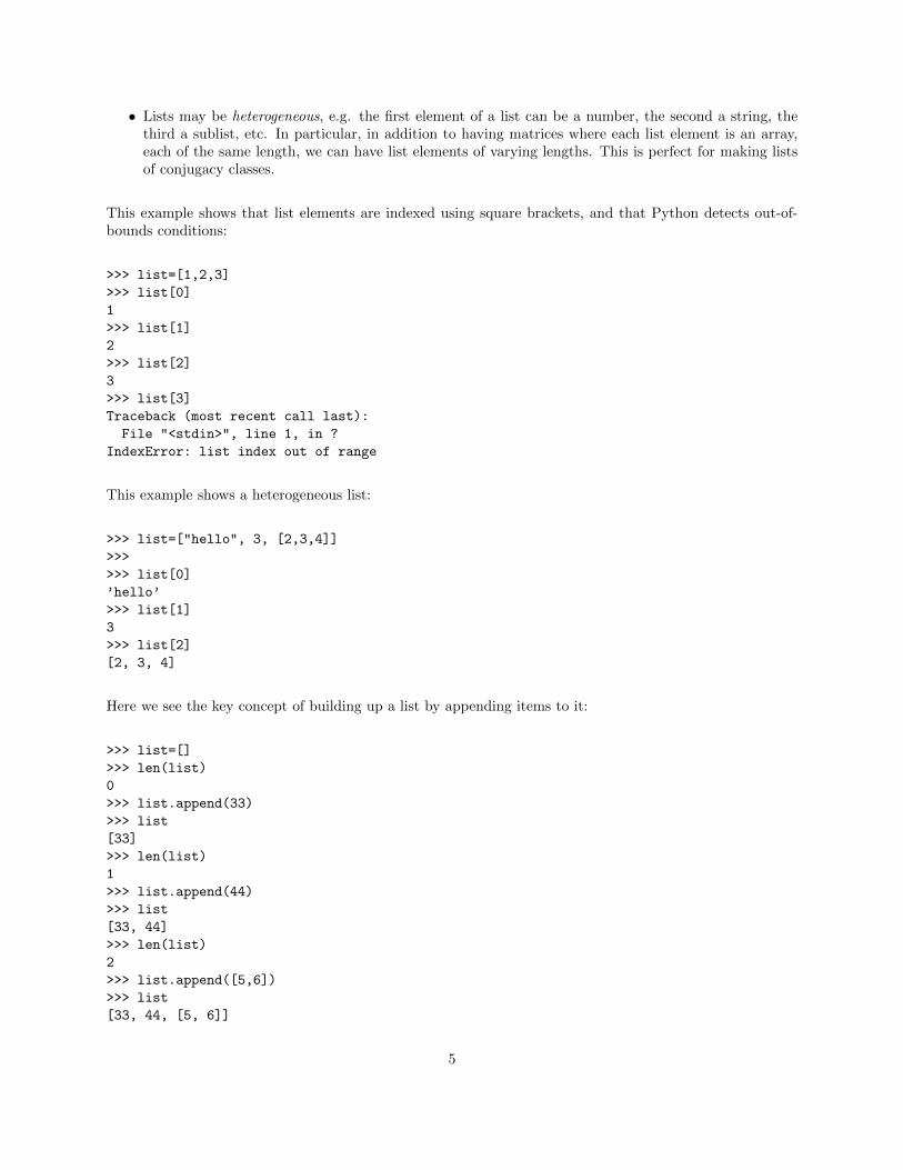
• Lists may be heterogeneous, e.g. the first element of a list can be a number, the second a string, thethird a sublist, etc. In particular, in addition to having matrices where each list element is an array,each of the same length, we can have list elements of varying lengths. This is perfect for making listsof conjugacy classes.

This example shows that list elements are indexed using square brackets, and that Python detects out-of-bounds conditions:

>>> list=[1,2,3]

>>> list[0]

1

>>> list[1]

2

>>> list[2]

3

>>> list[3]

Traceback (most recent call last):

File "<stdin>", line 1, in ?

IndexError: list index out of range

This example shows a heterogeneous list:

>>> list=["hello", 3, [2,3,4]]

>>>

>>> list[0]

’hello’

>>> list[1]

3

>>> list[2]

[2, 3, 4]

Here we see the key concept of building up a list by appending items to it:

>>> list=[]

>>> len(list)

0

>>> list.append(33)

>>> list

[33]

>>> len(list)

1

>>> list.append(44)

>>> list

[33, 44]

>>> len(list)

2

>>> list.append([5,6])

>>> list

[33, 44, [5, 6]]

5

>>> len(list)

3

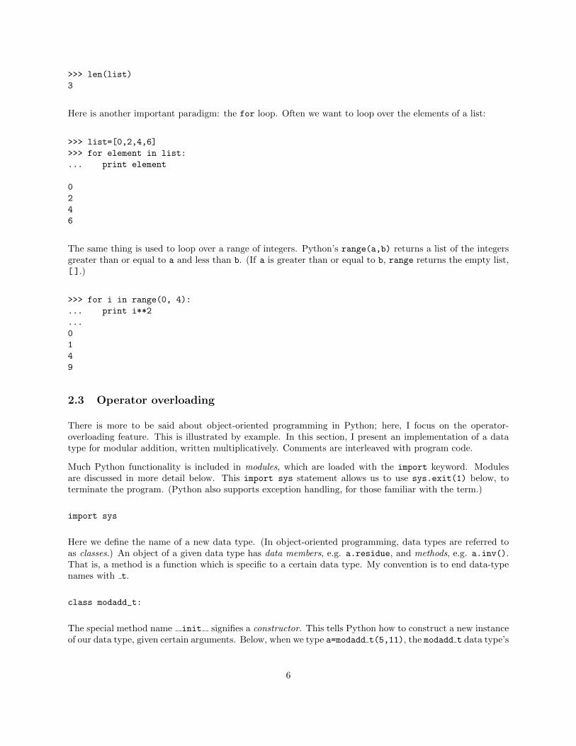
Here is another important paradigm: the for loop. Often we want to loop over the elements of a list:

>>> list=[0,2,4,6]

>>> for element in list:

... print element

0

2

4

6

The same thing is used to loop over a range of integers. Python’s range(a,b) returns a list of the integersgreater than or equal to a and less than b. (If a is greater than or equal to b, range returns the empty list,[ ].)

>>> for i in range(0, 4):

... print i**2

...

0

1

4

9

2.3 Operator overloading

There is more to be said about object-oriented programming in Python; here, I focus on the operator-overloading feature. This is illustrated by example. In this section, I present an implementation of a datatype for modular addition, written multiplicatively. Comments are interleaved with program code.

Much Python functionality is included in modules, which are loaded with the import keyword. Modulesare discussed in more detail below. This import sys statement allows us to use sys.exit(1) below, toterminate the program. (Python also supports exception handling, for those familiar with the term.)

import sys

Here we define the name of a new data type. (In object-oriented programming, data types are referred toas classes.) An object of a given data type has data members, e.g. a.residue, and methods, e.g. a.inv().That is, a method is a function which is specific to a certain data type. My convention is to end data-typenames with t.

class modadd_t:

The special method name init signifies a constructor. This tells Python how to construct a new instanceof our data type, given certain arguments. Below, when we type a=modadd t(5,11), the modadd t data type’s

6

init method will be invoked with 5 and 11 as the residue and modulus arguments, respectively. Thekeyword self is used by all methods. This is a technical detail.

More important is the statement with the percent sign. This is the modulus or remainder operator. What wedo here is reduce the residue mod n to a canonical representative, at the moment an object is constructed.This enables us to test for exact equality below.

def __init__(self, residue, modulus):

self.residue = residue % modulus

self.modulus = modulus

By defining a method with the special name mul , we instruct the Python interpreter what to do when itencounters statements of the form a * b, where a and b are instances of this data type.

# Use "*" for addition. Seems weird, but groups are abstracted

# multiplicatively in SACK.

def __mul__(a,b):

if (a.modulus != b.modulus):

print "Mixed moduli %d, %d" % (a, b)

sys.exit(1)

c = modadd_t(a.residue + b.residue, a.modulus)

return c

Likewise for eq and ne , which tell the Python interpreter what to do for a == b and a != b, whichis Python’s way of saying a = b and a 6= b respectively.

def __eq__(a,b):

if (a.residue != b.residue):

return 0

return 1

def __ne__(a,b):

return not (a == b)

The str method is another special one which tells the Python interpreter how to turn our objects intostrings, in particular for printing.

def __str__(self):

return str(self.residue)

Unlike mul , the name inv has no special significance to Python. However, all our data types will havean inv method, so we will be able to invert any element b by writing b.inv(), regardless of the data typeof b. Like the trailing t for data-type names, this is a SACK convention.

def inv(a):

c = modadd_t(-a.residue, a.modulus)

return c

Here is a little test routine. It prints 2 when invoked. The first and second lines result in the init

method being called; the third results in the mul method being called.

7

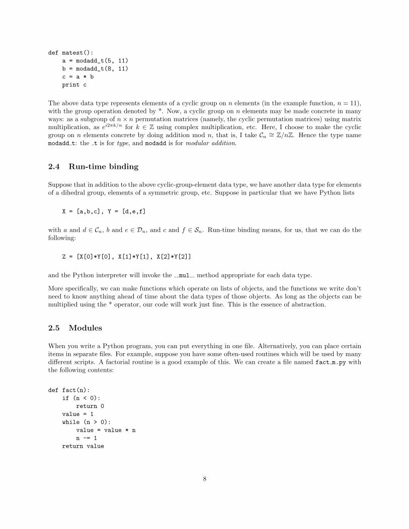
def matest():

a = modadd_t(5, 11)

b = modadd_t(8, 11)

c = a * b

print c

The above data type represents elements of a cyclic group on n elements (in the example function, n = 11),with the group operation denoted by *. Now, a cyclic group on n elements may be made concrete in manyways: as a subgroup of n× n permutation matrices (namely, the cyclic permutation matrices) using matrixmultiplication, as ei2πk/n for k ∈ Z using complex multiplication, etc. Here, I choose to make the cyclicgroup on n elements concrete by doing addition mod n, that is, I take Cn ∼= Z/nZ. Hence the type namemodadd t: the t is for type, and modadd is for modular addition.

2.4 Run-time binding

Suppose that in addition to the above cyclic-group-element data type, we have another data type for elementsof a dihedral group, elements of a symmetric group, etc. Suppose in particular that we have Python lists

X = [a,b,c], Y = [d,e,f]

with a and d ∈ Cn, b and e ∈ Dn, and c and f ∈ Sn. Run-time binding means, for us, that we can do thefollowing:

Z = [X[0]*Y[0], X[1]*Y[1], X[2]*Y[2]]

and the Python interpreter will invoke the mul method appropriate for each data type.

More specifically, we can make functions which operate on lists of objects, and the functions we write don’tneed to know anything ahead of time about the data types of those objects. As long as the objects can bemultiplied using the * operator, our code will work just fine. This is the essence of abstraction.

2.5 Modules

When you write a Python program, you can put everything in one file. Alternatively, you can place certainitems in separate files. For example, suppose you have some often-used routines which will be used by manydifferent scripts. A factorial routine is a good example of this. We can create a file named fact m.py withthe following contents:

def fact(n):

if (n < 0):

return 0

value = 1

while (n > 0):

value = value * n

n -= 1

return value

8

The trailing m is, again, my convention: it stands for module. Another program can use this routine bydoing two things: (1) import the module; (2) call the routine with module name, dot, function name. Forexample:

import fact_m

x = fact_m.fact(20)

Side note: The implementation of fact shown at the beginning of this document was recursive, since itcalled itself. The implementation shown just above is iterative, since it loops. This is akin to the differencebetween defining n! recursively via

n! =

{n · (n− 1)!, n > 01 n = 0

versus iteratively by

n! =

n∏k=1

k.

Above I noted that the inv() method is spelled the same for all data types, so that I can invert any elementa of any group using a.inv(). Likewise, for group-fill functions below, several modules will have a functionnamed get elements(). This way, we can put the name of a desired group into a variable called, say,group name, then get the contents by invoking group name.get elements().

3 Concrete groups

In this section, a few concrete groups are introduced, in addition to the cyclic group already examined.The key point is that for each concrete type, the operations idiosyncratic to that type are defined by theprogrammer. Then, in section 4, general-purpose code will be used to take care of group-theoretic operationswhich are independent of data type.

The data types to be discussed here include:

• Klein-four and unit-quaternion groups

• Metacyclic, dihedral, and generalized-quaternion groups

• Symmetric and alternating groups

Note that dihedral groups (symmetries of plane n-gons) could have been implemented as subgroups of Sn.In fact, all these small finite groups could be done this way. The point is that by implementing specific datatypes, we obtain more user-friendly input-output representations. For example, for V4, we will have elementsprinted simply as e, a, b, and c.

There are two levels of software needed for each group: (1) routines to deal with individual group elements,and (2) routines to construct a list of all the elements of a group.

3.1 V4 and Q8

For the Klein-four group, we observe that V4 ∼= Z2×Z2. It takes two bits to represent a Klein-four element.Addition mod 2 is done using the XOR operation, which is written with a caret.

9

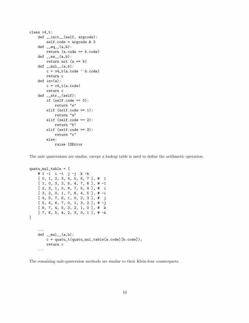
class v4_t:

def __init__(self, argcode):

self.code = argcode & 3

def __eq__(a,b):

return (a.code == b.code)

def __ne__(a,b):

return not (a == b)

def __mul__(a,b):

c = v4_t(a.code ^ b.code)

return c

def inv(a):

c = v4_t(a.code)

return c

def __str__(self):

if (self.code == 0):

return "e"

elif (self.code == 1):

return "a"

elif (self.code == 2):

return "b"

elif (self.code == 3):

return "c"

else:

raise IOError

The unit quaternions are similar, except a lookup table is used to define the arithmetic operation.

quatu_mul_table = [

# 1 -1 i -i j -j k -k

[ 0, 1, 2, 3, 4, 5, 6, 7 ], # 1

[ 1, 0, 3, 2, 5, 4, 7, 6 ], # -1

[ 2, 3, 1, 0, 6, 7, 5, 4 ], # i

[ 3, 2, 0, 1, 7, 6, 4, 5 ], # -i

[ 4, 5, 7, 6, 1, 0, 2, 3 ], # j

[ 5, 4, 6, 7, 0, 1, 3, 2 ], # -j

[ 6, 7, 4, 5, 3, 2, 1, 0 ], # k

[ 7, 6, 5, 4, 2, 3, 0, 1 ], # -k

]

...

def __mul__(a,b):

c = quatu_t(quatu_mul_table[a.code][b.code]);

return c

...

The remaining unit-quaternion methods are similar to their Klein-four counterparts.

10

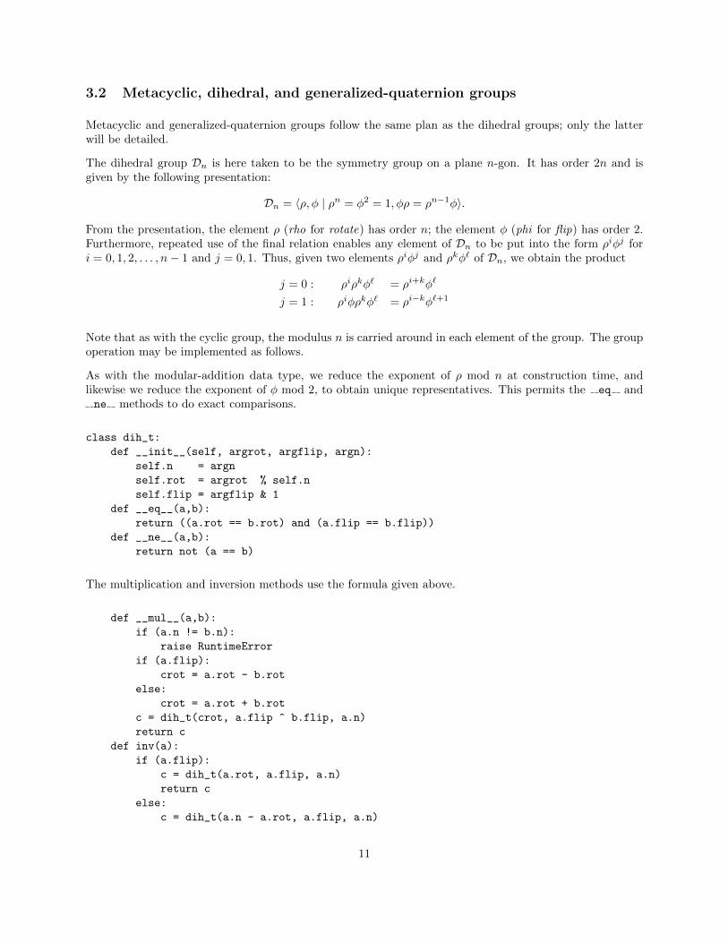
3.2 Metacyclic, dihedral, and generalized-quaternion groups

Metacyclic and generalized-quaternion groups follow the same plan as the dihedral groups; only the latterwill be detailed.

The dihedral group Dn is here taken to be the symmetry group on a plane n-gon. It has order 2n and isgiven by the following presentation:

Dn = 〈ρ, φ | ρn = φ2 = 1, φρ = ρn−1φ〉.

From the presentation, the element ρ (rho for rotate) has order n; the element φ (phi for flip) has order 2.Furthermore, repeated use of the final relation enables any element of Dn to be put into the form ρiφj fori = 0, 1, 2, . . . , n− 1 and j = 0, 1. Thus, given two elements ρiφj and ρkφ` of Dn, we obtain the product

j = 0 : ρiρkφ` = ρi+kφ`

j = 1 : ρiφρkφ` = ρi−kφ`+1

Note that as with the cyclic group, the modulus n is carried around in each element of the group. The groupoperation may be implemented as follows.

As with the modular-addition data type, we reduce the exponent of ρ mod n at construction time, andlikewise we reduce the exponent of φ mod 2, to obtain unique representatives. This permits the eq andne methods to do exact comparisons.

class dih_t:

def __init__(self, argrot, argflip, argn):

self.n = argn

self.rot = argrot % self.n

self.flip = argflip & 1

def __eq__(a,b):

return ((a.rot == b.rot) and (a.flip == b.flip))

def __ne__(a,b):

return not (a == b)

The multiplication and inversion methods use the formula given above.

def __mul__(a,b):

if (a.n != b.n):

raise RuntimeError

if (a.flip):

crot = a.rot - b.rot

else:

crot = a.rot + b.rot

c = dih_t(crot, a.flip ^ b.flip, a.n)

return c

def inv(a):

if (a.flip):

c = dih_t(a.rot, a.flip, a.n)

return c

else:

c = dih_t(a.n - a.rot, a.flip, a.n)

11

return c

def __str__(self):

return str(self.rot) + "," + str(self.flip)

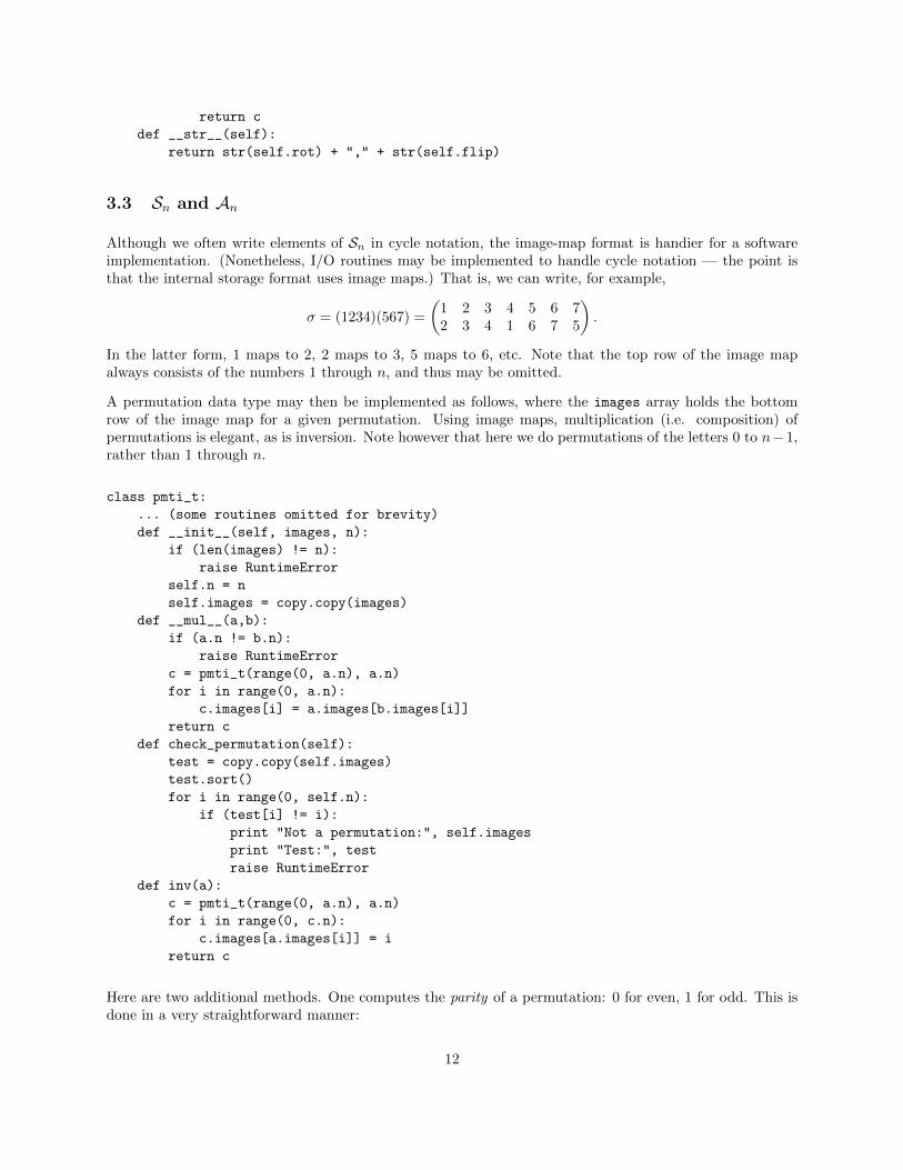
3.3 Sn and An

Although we often write elements of Sn in cycle notation, the image-map format is handier for a softwareimplementation. (Nonetheless, I/O routines may be implemented to handle cycle notation — the point isthat the internal storage format uses image maps.) That is, we can write, for example,

σ = (1234)(567) =

(1 2 3 4 5 6 72 3 4 1 6 7 5

).

In the latter form, 1 maps to 2, 2 maps to 3, 5 maps to 6, etc. Note that the top row of the image mapalways consists of the numbers 1 through n, and thus may be omitted.

A permutation data type may then be implemented as follows, where the images array holds the bottomrow of the image map for a given permutation. Using image maps, multiplication (i.e. composition) ofpermutations is elegant, as is inversion. Note however that here we do permutations of the letters 0 to n−1,rather than 1 through n.

class pmti_t:

... (some routines omitted for brevity)

def __init__(self, images, n):

if (len(images) != n):

raise RuntimeError

self.n = n

self.images = copy.copy(images)

def __mul__(a,b):

if (a.n != b.n):

raise RuntimeError

c = pmti_t(range(0, a.n), a.n)

for i in range(0, a.n):

c.images[i] = a.images[b.images[i]]

return c

def check_permutation(self):

test = copy.copy(self.images)

test.sort()

for i in range(0, self.n):

if (test[i] != i):

print "Not a permutation:", self.images

print "Test:", test

raise RuntimeError

def inv(a):

c = pmti_t(range(0, a.n), a.n)

for i in range(0, c.n):

c.images[a.images[i]] = i

return c

Here are two additional methods. One computes the parity of a permutation: 0 for even, 1 for odd. This isdone in a very straightforward manner:

12

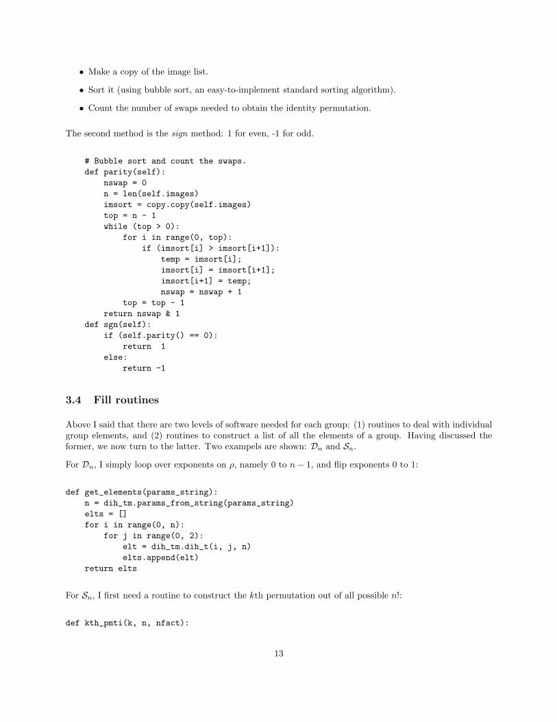
• Make a copy of the image list.

• Sort it (using bubble sort, an easy-to-implement standard sorting algorithm).

• Count the number of swaps needed to obtain the identity permutation.

The second method is the sign method: 1 for even, -1 for odd.

# Bubble sort and count the swaps.

def parity(self):

nswap = 0

n = len(self.images)

imsort = copy.copy(self.images)

top = n - 1

while (top > 0):

for i in range(0, top):

if (imsort[i] > imsort[i+1]):

temp = imsort[i];

imsort[i] = imsort[i+1];

imsort[i+1] = temp;

nswap = nswap + 1

top = top - 1

return nswap & 1

def sgn(self):

if (self.parity() == 0):

return 1

else:

return -1

3.4 Fill routines

Above I said that there are two levels of software needed for each group: (1) routines to deal with individualgroup elements, and (2) routines to construct a list of all the elements of a group. Having discussed theformer, we now turn to the latter. Two exampels are shown: Dn and Sn.

For Dn, I simply loop over exponents on ρ, namely 0 to n− 1, and flip exponents 0 to 1:

def get_elements(params_string):

n = dih_tm.params_from_string(params_string)

elts = []

for i in range(0, n):

for j in range(0, 2):

elt = dih_tm.dih_t(i, j, n)

elts.append(elt)

return elts

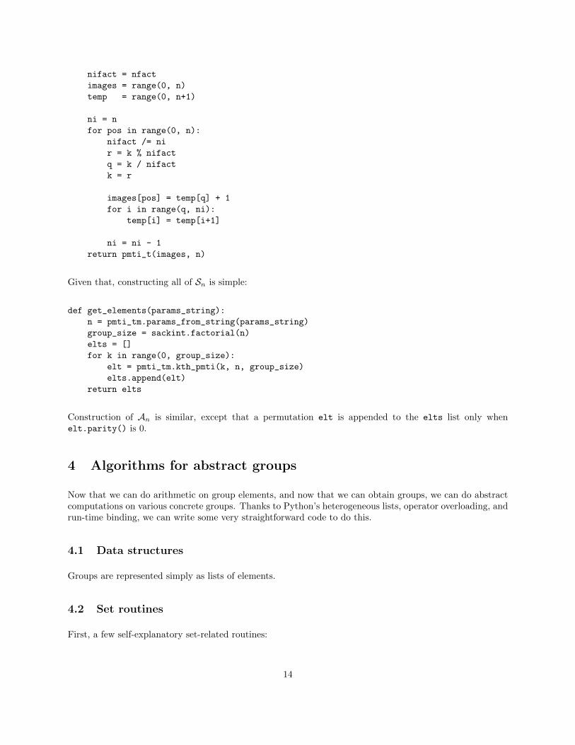
For Sn, I first need a routine to construct the kth permutation out of all possible n!:

def kth_pmti(k, n, nfact):

13

nifact = nfact

images = range(0, n)

temp = range(0, n+1)

ni = n

for pos in range(0, n):

nifact /= ni

r = k % nifact

q = k / nifact

k = r

images[pos] = temp[q] + 1

for i in range(q, ni):

temp[i] = temp[i+1]

ni = ni - 1

return pmti_t(images, n)

Given that, constructing all of Sn is simple:

def get_elements(params_string):

n = pmti_tm.params_from_string(params_string)

group_size = sackint.factorial(n)

elts = []

for k in range(0, group_size):

elt = pmti_tm.kth_pmti(k, n, group_size)

elts.append(elt)

return elts

Construction of An is similar, except that a permutation elt is appended to the elts list only whenelt.parity() is 0.

4 Algorithms for abstract groups

Now that we can do arithmetic on group elements, and now that we can obtain groups, we can do abstractcomputations on various concrete groups. Thanks to Python’s heterogeneous lists, operator overloading, andrun-time binding, we can write some very straightforward code to do this.

4.1 Data structures

Groups are represented simply as lists of elements.

4.2 Set routines

First, a few self-explanatory set-related routines:

14

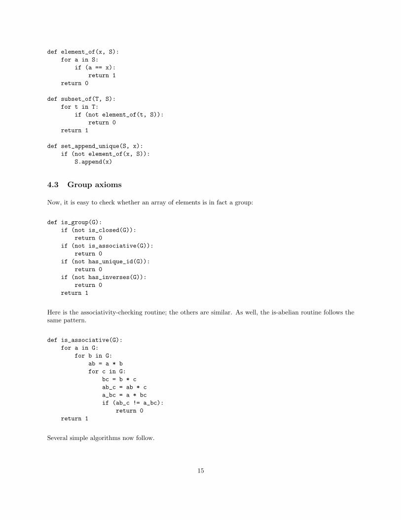
def element_of(x, S):

for a in S:

if (a == x):

return 1

return 0

def subset_of(T, S):

for t in T:

if (not element_of(t, S)):

return 0

return 1

def set_append_unique(S, x):

if (not element_of(x, S)):

S.append(x)

4.3 Group axioms

Now, it is easy to check whether an array of elements is in fact a group:

def is_group(G):

if (not is_closed(G)):

return 0

if (not is_associative(G)):

return 0

if (not has_unique_id(G)):

return 0

if (not has_inverses(G)):

return 0

return 1

Here is the associativity-checking routine; the others are similar. As well, the is-abelian routine follows thesame pattern.

def is_associative(G):

for a in G:

for b in G:

ab = a * b

for c in G:

bc = b * c

ab_c = ab * c

a_bc = a * bc

if (ab_c != a_bc):

return 0

return 1

Several simple algorithms now follow.

15

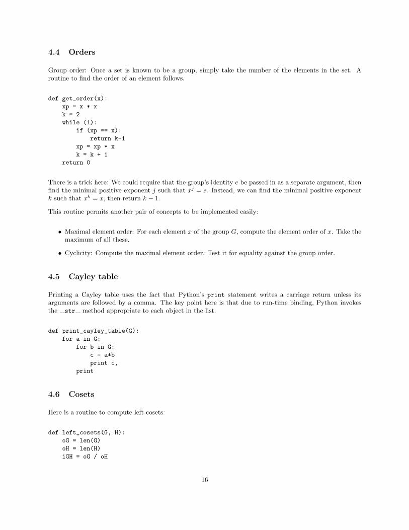
4.4 Orders

Group order: Once a set is known to be a group, simply take the number of the elements in the set. Aroutine to find the order of an element follows.

def get_order(x):

xp = x * x

k = 2

while (1):

if (xp == x):

return k-1

xp = xp * x

k = k + 1

return 0

There is a trick here: We could require that the group’s identity e be passed in as a separate argument, thenfind the minimal positive exponent j such that xj = e. Instead, we can find the minimal positive exponentk such that xk = x, then return k − 1.

This routine permits another pair of concepts to be implemented easily:

• Maximal element order: For each element x of the group G, compute the element order of x. Take themaximum of all these.

• Cyclicity: Compute the maximal element order. Test it for equality against the group order.

4.5 Cayley table

Printing a Cayley table uses the fact that Python’s print statement writes a carriage return unless itsarguments are followed by a comma. The key point here is that due to run-time binding, Python invokesthe str method appropriate to each object in the list.

def print_cayley_table(G):

for a in G:

for b in G:

c = a*b

print c,

print

4.6 Cosets

Here is a routine to compute left cosets:

def left_cosets(G, H):

oG = len(G)

oH = len(H)

iGH = oG / oH

16

... (error-checking here to make sure order of H divides order of G)

GH = []

for g in G:

gHe = range(0, oH)

for j in range(0, oH):

gHe[j] = g * H[j]

gH = coset(gHe)

set_append_unique(GH, gH)

return GH

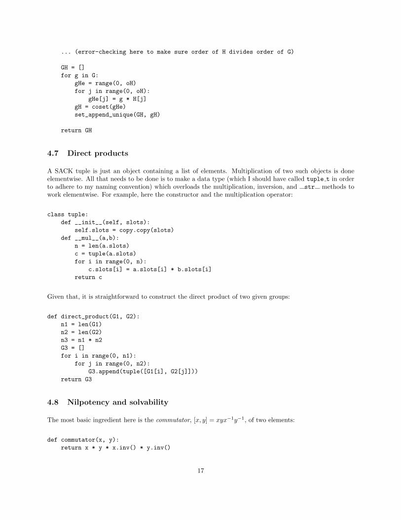
4.7 Direct products

A SACK tuple is just an object containing a list of elements. Multiplication of two such objects is doneelementwise. All that needs to be done is to make a data type (which I should have called tuple t in orderto adhere to my naming convention) which overloads the multiplication, inversion, and str methods towork elementwise. For example, here the constructor and the multiplication operator:

class tuple:

def __init__(self, slots):

self.slots = copy.copy(slots)

def __mul__(a,b):

n = len(a.slots)

c = tuple(a.slots)

for i in range(0, n):

c.slots[i] = a.slots[i] * b.slots[i]

return c

Given that, it is straightforward to construct the direct product of two given groups:

def direct_product(G1, G2):

n1 = len(G1)

n2 = len(G2)

n3 = n1 * n2

G3 = []

for i in range(0, n1):

for j in range(0, n2):

G3.append(tuple([G1[i], G2[j]]))

return G3

4.8 Nilpotency and solvability

The most basic ingredient here is the commutator, [x, y] = xyx−1y−1, of two elements:

def commutator(x, y):

return x * y * x.inv() * y.inv()

17

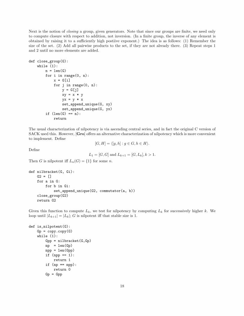
Next is the notion of closing a group, given generators. Note that since our groups are finite, we need onlyto compute closure with respect to addition, not inversion. (In a finite group, the inverse of any element isobtained by raising it to a sufficiently high postiive exponent.) The idea is as follows: (1) Remember thesize of the set. (2) Add all pairwise products to the set, if they are not already there. (3) Repeat steps 1and 2 until no more elements are added.

def close_group(G):

while (1):

n = len(G)

for i in range(0, n):

x = G[i]

for j in range(0, n):

y = G[j]

xy = x * y

yx = y * x

set_append_unique(G, xy)

set_append_unique(G, yx)

if (len(G) == n):

return

The usual characterization of nilpotency is via ascending central series, and in fact the original C version ofSACK used this. However, [Gro] offers an alternative characterization of nilpotency which is more convenientto implement. Define

[G,H] = 〈[g, h] : g ∈ G, h ∈ H〉.Define

L1 = [G,G] and Lk+1 = [G,Lk], k > 1.

Then G is nilpotent iff Ln(G) = {1} for some n.

def nilbracket(G, Gi):

G2 = []

for a in G:

for b in Gi:

set_append_unique(G2, commutator(a, b))

close_group(G2)

return G2

Given this function to compute Lk, we test for nilpotency by computing Lk for successively higher k. Weloop until |Lk+1| = |Lk|; G is nilpotent iff that stable size is 1.

def is_nilpotent(G):

Gp = copy.copy(G)

while (1):

Gpp = nilbracket(G,Gp)

np = len(Gp)

npp = len(Gpp)

if (npp == 1):

return 1

if (np == npp):

return 0

Gp = Gpp

18

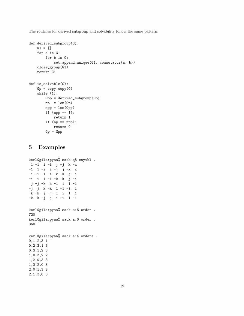
The routines for derived subgroup and solvability follow the same pattern:

def derived_subgroup(G):

G1 = []

for a in G:

for b in G:

set_append_unique(G1, commutator(a, b))

close_group(G1)

return G1

def is_solvable(G):

Gp = copy.copy(G)

while (1):

Gpp = derived_subgroup(Gp)

np = len(Gp)

npp = len(Gpp)

if (npp == 1):

return 1

if (np == npp):

return 0

Gp = Gpp

5 Examples

kerl@gila:pyaa% sack q8 caytbl .

1 -1 i -i j -j k -k

-1 1 -i i -j j -k k

i -i -1 1 k -k -j j

-i i 1 -1 -k k j -j

j -j -k k -1 1 i -i

-j j k -k 1 -1 -i i

k -k j -j -i i -1 1

-k k -j j i -i 1 -1

kerl@gila:pyaa% sack s:6 order .

720

kerl@gila:pyaa% sack a:6 order .

360

kerl@gila:pyaa% sack a:4 orders .

0,1,2,3 1

0,2,3,1 3

0,3,1,2 3

1,0,3,2 2

1,2,0,3 3

1,3,2,0 3

2,0,1,3 3

2,1,3,0 3

19

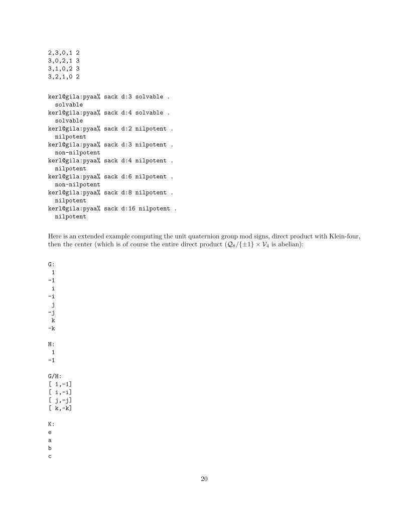
2,3,0,1 2

3,0,2,1 3

3,1,0,2 3

3,2,1,0 2

kerl@gila:pyaa% sack d:3 solvable .

solvable

kerl@gila:pyaa% sack d:4 solvable .

solvable

kerl@gila:pyaa% sack d:2 nilpotent .

nilpotent

kerl@gila:pyaa% sack d:3 nilpotent .

non-nilpotent

kerl@gila:pyaa% sack d:4 nilpotent .

nilpotent

kerl@gila:pyaa% sack d:6 nilpotent .

non-nilpotent

kerl@gila:pyaa% sack d:8 nilpotent .

nilpotent

kerl@gila:pyaa% sack d:16 nilpotent .

nilpotent

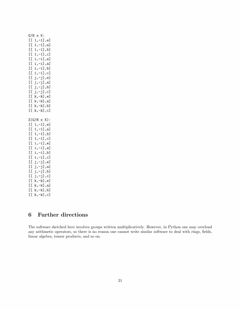
Here is an extended example computing the unit quaternion group mod signs, direct product with Klein-four,then the center (which is of course the entire direct product (Q8/{±1} × V4 is abelian):

G:

1

-1

i

-i

j

-j

k

-k

H:

1

-1

G/H:

[ 1,-1]

[ i,-i]

[ j,-j]

[ k,-k]

K:

e

a

b

c

20

G/H x K:

[[ 1,-1],e]

[[ 1,-1],a]

[[ 1,-1],b]

[[ 1,-1],c]

[[ i,-i],e]

[[ i,-i],a]

[[ i,-i],b]

[[ i,-i],c]

[[ j,-j],e]

[[ j,-j],a]

[[ j,-j],b]

[[ j,-j],c]

[[ k,-k],e]

[[ k,-k],a]

[[ k,-k],b]

[[ k,-k],c]

Z(G/H x K):

[[ 1,-1],e]

[[ 1,-1],a]

[[ 1,-1],b]

[[ 1,-1],c]

[[ i,-i],e]

[[ i,-i],a]

[[ i,-i],b]

[[ i,-i],c]

[[ j,-j],e]

[[ j,-j],a]

[[ j,-j],b]

[[ j,-j],c]

[[ k,-k],e]

[[ k,-k],a]

[[ k,-k],b]

[[ k,-k],c]

6 Further directions

The software sketched here involves groups written multiplicatively. However, in Python one may overloadany arithmetic operators, so there is no reason one cannot write similar software to deal with rings, fields,linear algebra, tensor products, and so on.

21

References

[Gro] L.C. Grove. Algebra Dover, 2004.

[Lut] Lutz, M. and Ascher, D. Learning Python (2nd ed.). O’Reilly, 2004.

22