Computer Graphics

Shi-Min Hu

Tsinghua University

Bézier Curves and Surfaces

• Parametric curves and surface: Some

Concepts

• Bézier Cuvres: Concept and properties

• Bézier surfaces: Rectangular and

Triangular

• Conversion of Rectangular and Triangular

Bézier surfaces

Parametric curves and surface

• In Graphics, we usually design a scene and

then generate realistic image by using

rendering equation.

• It’s necessary to introduce geometric

modeling for scene design.

• How to represent 3D shapes (models) in

computer?

History of Geometric Modeling

• Surface Modeling :

– In 1962, Pierre Bézier, an engineer of French

Renault Car company, propose a new kind of

curve representation, and finally developed a

system UNISURF for car surface design in 1972.

• Pierre Etienne Bezier was born on September 1, 1910 in

Paris. Son and grandson of engineers

• He entered the Ecole Superieure d'Electricite and earnt a

second degree in electrical engineering in 1931. In 1977,

46 years later, he received his DSc degree in mathematics

from the University of Paris.

• In 1933, aged 23, Bezier entered Renault and worked for

this company for 42 years.

• Bezier's academic career began in 1968 when he became

Professor of Production Engineering at the Conservatoire

National des Arts et Metiers. He held this position until

1979.

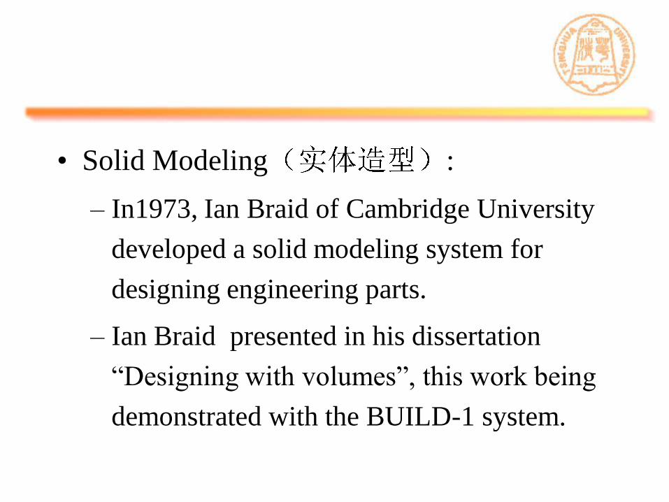
• Solid Modeling :

– In1973, Ian Braid of Cambridge University

developed a solid modeling system for

designing engineering parts.

– Ian Braid presented in his dissertation

“Designing with volumes”, this work being

demonstrated with the BUILD-1 system.

How to represent a curve?

• There are three major types of object

representation:

– Explicit representation: the explicit form of a

curve in 2D gives the value of one variable,

the dependent variable, in terms of the other,

the independent variable. In x, y space, we

may write

– For the line, we usually write

( )y f x

y mx h

– Implicit representation: In two dimensions, an

implicit curve can be represented by the equation

– For the line

– For the circle

2 2 2 0x y r

( , ) 0f x y

0ax by c

– Parametric form: The parametric form of a curve

expresses the value of each spatial variable for

points on the curve in terms of an independent

variable , the parameter.

– In 3D, we have three explicit functions

t

( )

( )

( )

x x t

y y t

z z t

– One of the advantages of the parametric form is

that it is the same in two and three dimensions. In

the former case, we simply drop the equation for

z.

– A useful representation of the parametric form is

to visualize the locus of points

( )

being drawn as t varies.

( ) [ ( ), ( ), ( )]TP t x t y t z t

– We can think of the derivative

As the velocity with which the curve is traced out

and points in direction tangent to the curve.

( )

( ) ( )

( )

dx t

dt

dP t dy t

dt dt

dz t

dt

Parametric polynomial curves

• Parametric curves are not unique. A given curve or

surface can be represented in many ways, but we

shall find that parametric forms in which the

functions are polynomials in t.

• A polynomial parametric curve of degree 3 is of

form

• It was known as Ferguson curve, and was used for

airplane design in earlier in USA.

3 2( )P t at bt ct d

• But Ferguson curve is not straightforward,

even the coefficients a, b, c, d are given, it’s

still hard to imagine the shape of the curve.

Bézier Cuvres: Concept and

properties

• Pierre Bézier proposed a method to represent

a curve in terms of connected vectors.

,

0

1 1,

1

( ) ( )

1, 0,

( ) ( ) (1 ) 1

( 1)!

n

i n i

i

i i ni n

i

V t f t A

i

f t t d t

i dt t

• Curve can be designed interactively?

– Curve are generated according to the control

net (those connected vectors)

– We may change vectors to modify the curve

– See demo: curvesystem.exe

• However, such a definition is unintelligible

• 1972, Forrest published his famous paper in

Computer Aided Design journal,

– he pointed out that, Bézier curve can be defined

in terms of points with help of Bernstein

Polynomials.

– Liang Youdong, Chang Gengzhe, Liu Dingyuan

– P Bézier was passed away in 1999, CAGD

published a Special issue for him in 2001

CAGD special issue

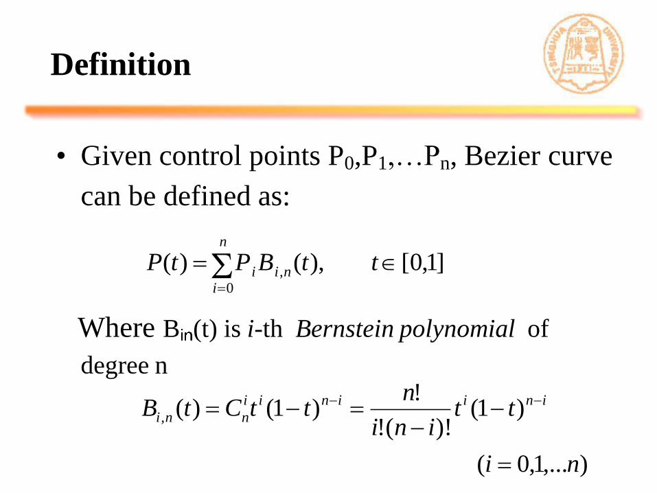
Definition

• Given control points P0,P1,…Pn, Bezier curve

can be defined as:

Where B (t) is i-th Bernstein polynomial of

degree n

]1,0[),()( ,0

ttBPtP nii

n

i

),...1,0(

)1()!(!

!)1()(,

ni

ttini

nttCtB iniinii

nni

Three Bezier curves

Degree two Degree three

Degree four

Property of Bernstein polynomial

• Non-negative ( )

• End point

,

0 0,1( )

0 (0,1), 1,2, , 1;i n

tB t

t i n

otherswise

niB

otherswise

iB

ni

ni

0

)(1)1(

0

)0(1)0(

,

,

• Unity

– Proof: According to Binomial

Theorem( ), we have

,

0

( ) 1 (0,1)n

i n

i

B t t

n

i

n

i

ninii

nni ttttCtB0 0

, 1])1[()1()(

• Symmetry ( )

– Proof:

, ,(1 ) ( )i n n i nB t B t

)1()1(

)1()]1(1[)(

,

)(

,

tBttC

ttCtB

ni

inii

n

ininnin

nnin

• Recursive ( )

– This means that Bernstein Polynomial of degree

n is a linear combination of two Bernstein

Polynomial of degree n-1.

),...,1,0(

),()()1()( 1,11,,

ni

ttBtBttB ninini

)()()1(

)1()1()1(

)1()()1()(

1,11,

)1()1(11

1

)1(

1

1

11,

ttBtBt

tttCttCt

ttCCttCtB

nini

inii

n

inii

n

inii

n

i

n

inii

nni

• Derivation ( )

• Maximum

– has a unique local maximum on the

interval [0,1] at x = i/n

;,,1,0

)],()([)( 1,1,1,

ni

tBtBntB ninini

B ti n, ( )

• degree raising formula

)(1

1)()

11()(

)(1

1)(

)()1

1()()1(

1,11,,

1,1,

1,,

tBn

itB

n

itB

tBn

ittB

tBn

itBt

ninini

nini

nini

• Integral

1

0,

1

1)(

ntB ni

Property of Bezier curve

• End point properties

– Position of end point

• According to the end position’s property of

Bernstein polynomial, We have

• So the start point and end point of Bezier curve

coincide with start point and end point of the

control polygon.

0(0) , (1) ,nP P P P

– Tangent Vector

• Since

• We have

• This implies the tangent vector of the curve at the

start and end points is the same with the direction

of the first and last edges of the control polygon

1

0

1,1,1

' )]()([)(n

i

ninii tBtBPntP

1 0 1'(0) ( ), '(1) ( )n nP n P P P n P P

– Second Derivative

So we have

By the Curvature formula, we have

2''

2 1 , 2

0

( ) ( 1) ( 2 ) ( )n

i i i i n

i

P t n n P P P B t

)2)(1()0( 012

" PPPnnP

)2)(1()1( 21

"

nnn PPPnnP

3

01

1201 )()(1)0(

PP

PPPP

n

nk

3

1

121 )()(1)1(

nn

nnnn

PP

PPPP

n

nk

– Difference form of k-th Derivative

• The high-order forward difference vector is

recursively defined by low-order forward

difference vector:

]1,0[)()!(

!)(

0

,

ttBPkn

ntP

kn

i

knii

kk

i

k

i

k

i

k PPP 1

1

1

ii PP 0

• Symmetry( )

– The curve with control points

remain the shape of the curve P(t), but with

opposite direction.

* , ( 0,1,..., )i n iP P i n

*

, , ,

0 0 0

,

0

*( ) ( ) ( ) (1 )

(1 ), [0,1]

n n n

i i n n i i n n i n i n

i i i

n

i i n

i

C t P B t P B t P B t

PB t t

• Convex hull ( ) Property

– By

and

– The curve P(t) is inside the convex hull of the

control polygon

n

i

ni tB0

, 1)(

),,1,0,10(1)(0 , nittB ni

• Geometric invariance ( )

– It means that some geometry property doesn’t

change with Coordinates varying.

– The position and shape of Bezier curve are

dependent on vertex Pi of control polygon, but

not the Coordinates.

de Casteljau Algorithm

• In industry application, it’s required to

evaluate a point on the curve at parameter t.

• We didn’t evaluate the value by the Bezier

Curve Equation, but use a recursive

algorithm, which is

numerical stable.

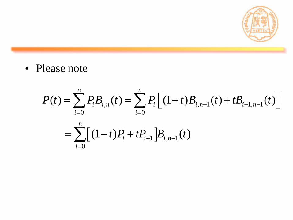
• Please note

, , 1 1, 1

0 0

1 , 1

0

( ) ( ) (1 ) ( ) ( )

(1 ) ( )

n n

i i n i i n i n

i i

n

i i i n

i

P t PB t P t B t tB t

t P tP B t

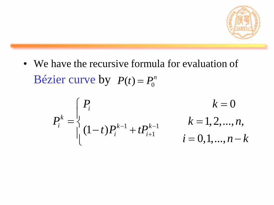
• We have the recursive formula for evaluation of

Bézier curve by

1 1

1

0

1,2,..., ,(1 )

0,1,...,

i

k

i k k

i i

P k

P k nt P tP

i n k

0( ) nP t P

• When n = 3, the recursive procedure is

illustrated by the following figure:

0P

1P

2P

3P

1

0P

1

1P

1

2P

2

0P

2

1P 3

0P

n

iP

)3/1(3

0 PP

0P

1P2P

3P

1

0P

1

1P1

2P2

0P

2

1P

Geometric continuity

• In CAD applications, it’s not encouraged to design

a curve by high degree Bézier curve.

• It’s common to use lower degree Bézier curves with

smooth connections.

• Can we use traditional concept of continuity?

1 00

1 0 1 00

, 0 1 3

( )2( )

1 , 1 23 3

V VV t t

tV V V V

V t t

• Please note

• This means the function is not continuous.

• But the function is actually a straight line.

• Such a fact implies traditional concept of

continuous is not suitable for describing smoothness

of shapes in CAD and Graphics.

• This is why we use “Geometric continuity”

• Liu and Liang ( )

013

1)1( VV 01

3

2)1( VV

• Given two Bezier Curves defined by control points

and respectively

• Two curves share an end point, and :

11, jjjiii QQbPPa

b

PP

P

P

a

a P

Q

Q

bQ

Q(t)

( 0,1, , )iP i n ( 0,1, , )jQ j m

– continuous

– continuous

and Pn-1 Pn = Q0, Q1 are collinear,

– continuous (curvature continuous )

)1()1()0( '"2" PPQ

)( 110 nn PPQQ

2

2

1

22

21

2211

2

nnn PP

nP

nQ

0G 0nP Q

1G

2G

Degree raising/elevation

• Degree raising means that adding control

points to raise the degree of the Bézier curves,

but the shape and direction of the curve remain

unchanged.

– Degree raising increases the flexibility of shape

control.

– After degree raising, control points are changed.

– How to raising the degree of a polynomial? Bézier

curves?

• Please note

• We have the degree raising formula

, ,

0 0

1

1 , 1

0

( ) ( ) (1 ) ( )

1( )

1 1

n n

i i n i i n

i i

n

i i i n

i

P t PB t P t t B t

n i iP P B t

n n

)1,,1,0(1

11

1

*

niP

n

iP

n

iP iii

• The above formula illustrates

– The new control points are linear combination of

the old control points with Coefficient i/(n+1).

– The new control polygon is inside the convex

hull of old control polygon.

– The new control polygon is nearer to the curve.

• Demo: curve-system

Degree reduction

• Degree reduction is the opposite of degree

raising

– Can we reduce the degree of a polynomial without

change of shapes?

– Degree reduction is to find a curve defined by new

control points with minimum error

)1,,1,0(* niPi

– Suppose Pi is result of degree raising Pi*:

– We can get two recursive formula

*

1

*

iii Pn

iP

n

inP

## 1 0,1, , 1i i

i

nP iPP i n

n i

1,,1,)( *

*

1

nnii

PinnPP ii

i

• Then we have two kinds of degree reduction

schemes

– Forrest (1972)

– Farin (1983)

1,,12

1,

2

1,,1,0,

ˆ*

#

nn

iP

niP

P

i

i

i

*#

1)

11(ˆ

iii Pn

iP

n

iP

• Reference for accurate degree reduction

– M. A. Watkins and A. J. Worsey, Degree reduction of

Bézier curves, Computer Aided Design, 20(7), 1988, 398-

405

– Approximate degree

reduction of Bezier curves, Tsinghua Science and

Technology, No.2, 1998, 997-1000. (was reported in

national CAGD conference, 1993)

– Degree reduction of B-

spline curves, Computer Aided Geometric Design, 2001,

Vol. 13, NO. 2, 2001, 117-127.

Bezier surface

• Rectangular Bézier Surface

– Suppose is

control points, a degree rectangular Bezier

surface can be defined in the form of tensor

product

where and are

Bernstein polynomial.

),,1,0;,,1,0( mjnPij )1()1( mnnm

]1,0[,)()(),(0 0

,,

vuvBuBPvuPm

i

n

j

njmiij

imii

mmi uuCuB )1()(,

jnjj

nni vvCvB )1()(,

– Bézier Surfaces by matrix representation

)(

)(

)(

)(,),(),(),(

,

,1

,0

10

11110

00100

,,1,0

vB

vB

vB

PPP

PPP

PPP

uBuBuBvuP

mn

m

m

nmnn

m

m

nmnn

• Properties of rectangular

– Bézier Surface hold similar properties of Bézier

curves :

• The four corners of control net are also the corners

of the Bézier surface.

• The triangles

give tangent plane at 4 corners.

101000 PPP1,01 nnon PPP nmnmmn PPP ,11, 10,10 mmm PPP

00)0,0( PP 0)0,1( mPP nPP 0)1,0( mnPP )1,1(

– Geometric invariance

– Symmetry

– Convex hull

10P20P

01P

11P21P

31P

02P 22P12P

32P

13P23P

00)0,0( PP

30)0,1( PP

03)1,0( PP 33)1,1( PP

)0,(uP

)1,(uP

),0( vP

),1( vP

• Geometric continuity

– Given two degree m*n Bézier surfaces with

control points Pij and Qij:

)()(),(

)()(),(

,

0 0

,

0 0

,,

vBuBQvuQ

vBuBPvuP

nj

m

i

n

j

miij

m

i

n

j

njmiij

]1,0[, vu

),( vuP

),( vuQ

)0,0(P

)1,0(P

)0,1(Q

)1,1(Q

)0,0()0,1( QP

)1,0()1,1( QP

– Conditions of G0 continuous:

i.e.,

– Conditions of G1 continuous:

),0(),1( vQvP

),,1,0(,0 miQP ini

),1()(),1()(),0( vPvvPvvQ vuu

• de Casteljau algorithm

– De Casteljau algorithm of Bézier curves can be

extended for surfaces. Given control points

and parameter (u,v).

we have

),,1,0;,,1,0( njmiPij

, .

, , , 00

0 0

( , ) ( ) ( )

, [0,1]

m k n lk l m n

i j i m j n

i j

P u v P B u B v P

u v

are defined by following recursive formulas

Or

);,,2,1()1(

),,2,1;0()1(

)0(

,1

0,1

,1

0

1,0

1,

1,0,

nlmkuPPu

nlkvPPv

lkP

Pnk

i

nk

i

l

ji

l

ij

ij

lk

ij

),,2,1,()1(

)0;,,2,1()1(

)0(

1,

1,0

1,

,0

0,1

,1

0,1,

,

nlmkvPPv

lmkuPPu

lkP

Plm

j

lm

j

k

ji

k

ij

ij

lk

ji

,

,

k l

i jP

• Straightforward interpretation of de Casteljau

algorithm

m

i

mi

n

j

njij

m

i

n

j

njmiij

uBvBP

vBuBPvuP

0

,

0

,

0 0

,,

)()(

)()(),(

• Triangular Bézier surfaces

– Triangular Bézier surfaces are defined over

triangles, not squares.

– Barycentric coordinates (u,v,w) are used for the

definition of triangular Bézier surfaces .

iu

jv),( ji vuP

)0,(uP

)1,(uP

),0( vP),1( vP

),,0( wvP

),0,( wuP

)0,,( vuP),,( kji wvuP

),,( kji wvu

• Bernstein Base Function:

Where i+j+k=1 and i,j,k>=0.

– There are degree n Bernstein Base

functions.

]1,0[,,!!!

!),,(,, wvuwvu

kji

nwvuB kji

kji

)2)(1(2

1 nn

22

020 vB

vwB 22

011 uvB 22

110

22

002 wB uwB 22

101 22

200 uB

– Properties of non-negative and unity

– Recursive:

, ,

, ,

( , , ) 0

( , , ) 1

n

i j k

n

i j k

i j k n

B u v w

B u v w

),,(

),,(),,(),,(

1

1,,

1

,1,

1

,,1,,

wvuwB

wvuvBwvuuBwvuB

n

kji

n

kji

n

kji

n

kji

• Definition of triangular Bézier surfaces

, , , ,

, , , ,

0 0

( , , ) ( , , )

( , , )

, , 0, 1

n

i j k i j k

i j k n

n n in

i j k i j k

i j

P u v w P B u v w

P B u v w

u v w u v w

• de Casteljau Algorithm

1,,,1,,,1,, kjikjikjikji wPvPuPP

Conversion of Rectangular and

Triangular Bézier surfaces

• Because the rectangular and the triangular

patches use different base function, When

they are used in the same CAD system,

there will be some problem. So we

introduce the conversion between them.

• A triangular surface can be represented as

one degenerate rectangular surfaces or three

non-degenerate rectangular surfaces

• To a degenerate rectangular surface

,,,1,0,

,

1

0

21

1

0

ni

T

T

T

AAA

P

P

P

ini

i

i

i

in

i

i

is a degree raising operator:),1,0( niAi

kk

k

knkn

kn

kn

kn

kn

kn

kn

kn

A

)1(100001

1

1000

001

1

1

20

00011

100001

Shi-Min, Hu Conversion between triangular and rectangular Bezier

patches, Computer Aided Geometric Design, 2001, 18(7), 667-671.

• To three rectangular surfaces

– Domain decomposition

1P2P

3P

P1D

2D

3D

)1,0(

),0(1 dP

)0,0(O )0,(3 bP

),( caP

2P

U

V

1D

3D

2D

)0,1(

• some operator

– Identiy operator:

– Shifting operator:

– Difference operator:

• With help of those operators, we can rewrite

triangular Bézier surfaces as

ijij TITI :

1,2,11 ,: jiijjiiji TTETTEE

ijjiijijjiiji TTTTTT 1,2,11 ,:

1 2 00

1 2 00

( , ) ( (1 ) )

( )

n

n

T u v uE vE u v I T

u v I T

• The control points defined over can be

obtained by1D

CAGD 1996

ACM SIGGRAPH

• Popup: Automatic Paper Architectures from

3D Models ( )

– Given a 3D architectural model with user-specified

backdrop and ground (left), our algorithm automatically

creates a paper architecture approximating the model

(mid-right, with the planar layout in mid-left), which

can be physically engineered and popped-up (right).

• Finding Approximately Repeated Scene

Elements for Image Editing

– We propose a novel framework where simple

user input in the form of 8 scribbles are used to

guide detection and extraction of such repeated

9 elements

Thank You!