computational modeling of thermodynamic effects...
TRANSCRIPT
COMPUTATIONAL MODELING OF THERMODYNAMIC EFFECTS IN
CRYOGENIC CAVITATION
By
YOGEN UTTURKAR
A DISSERTATION PRESENTED TO THE GRADUATE SCHOOL OF THE UNIVERSITY OF FLORIDA IN PARTIAL FULFILLMENT
OF THE REQUIREMENTS FOR THE DEGREE OF DOCTOR OF PHILOSOPHY
UNIVERSITY OF FLORIDA
2005

Copyright 2005
by
Yogen Utturkar

To my wife and parents

iv
ACKNOWLEDGMENTS
I am grateful to several individuals for their support in my dissertation work. The
greater part of this work was made possible by the instruction of my teachers, and the
love and support of my family and friends. It is with my heartfelt gratitude that I
acknowledge each of them.
Firstly, I would like to express sincere thanks and appreciation to my advisor, Dr.
Wei Shyy, for his excellent guidance, support, trust, and patience throughout my doctoral
studies. I am very grateful for his remarkable wisdom, thought-provoking ideas, and
critical questions during the course of my research work. I thank him for encouraging,
motivating, and always prodding me to perform beyond my own limits. Secondly, I
would like to express sincere gratitude towards my co-advisor, Dr. Nagaraj Arakere, for
his firm support and caring attitude during some difficult times in my graduate studies. I
also would like to express my appreciation to the members of my dissertation committee
Dr. Louis Cattafesta, Dr. James Klausner, and Dr. Don Slinn, for their valuable
comments and expertise to better my work. I deeply thank Dr. Siddharth Thakur (ST) for
providing me substantial assistance with the STREAM code and for his cordial
suggestions on research work and career planning.
My thanks go to all the members of our lab, with whom I have had the privilege to
work. Due to the presence of all these wonderful people, work is more enjoyable. In
particular, it was a delightful experience to collaborate with Jiongyang Wu, Tushar Goel,
and Baoning Zhang on various research topics.
v
I would like to express my deepest gratitude towards my family members. My
parents have always provided me unconditional love. They have always given top
priority to my education, which made it possible for me to pursue graduate studies in the
United States. I would like to thank my grandparents for their selfless affection and
loving attitude during my early years. My wife’s parents and her sister’s family have
been extremely supportive throughout my graduate education. I greatly appreciate their
trust in my abilities.
Last but never least, I am thankful beyond words to my wife, Neeti Pathare.
Together, we have walked through this memorable, cherishable, and joyful journey of
graduate education. Her honest and unfaltering love has been my most precious
possession all these times. I thank her for standing besides me every time and every
where. To Neeti and my parents, I dedicate this thesis!
vi
TABLE OF CONTENTS page
ACKNOWLEDGMENTS ................................................................................................. iv
LIST OF TABLES............................................................................................................. ix
LIST OF FIGURES .............................................................................................................x
LIST OF SYMBOLS ....................................................................................................... xiv
ABSTRACT................................................................................................................... xviii
CHAPTER
1 INTRODUCTION AND RESEARCH SCOPE ...........................................................1
1.1 Types of Cavitation............................................................................................2 1.2 Cavitation in Cryogenic Fluids – Thermal Effect..............................................4 1.3 Contributions of the Current Study....................................................................8
2 LITERATURE REVIEW .............................................................................................9
2.1 General Review of Recent Studies .........................................................................9 2.2 Modeling Thermal Effects of Cavitation..............................................................19
2.2.1 Scaling Laws ..............................................................................................19 2.2.2 Experimental Studies..................................................................................24 2.2.3 Numerical Modeling of Thermal Effects ...................................................27
3 STEADY STATE COMPUTATIONS.......................................................................33
3.1 Governing Equations ............................................................................................33 3.1.1. Cavitation Modeling..................................................................................35
3.1.1.1 Merkle et al. Model ..........................................................................35 3.1.1.2 Sharp Interfacial Dynamics Model (IDM) .......................................35 3.1.1.3 Mushy Interfacial Dynamics Model (IDM) .....................................37
3.1.2 Turbulence Modeling .................................................................................40 3.1.3 Speed of Sound (SoS) Modeling ................................................................41 3.1.4 Thermal Modeling ......................................................................................42
3.1.4.1 Fluid property update .......................................................................42 3.1.4.2 Evaporative cooling effects ..............................................................43
vii
3.1.5 Boundary Conditions..................................................................................44 3.2 Results and Discussion .........................................................................................45
3.2.1 Cavitation in Non-cryogenic Fluids ...........................................................45 3.2.2 Cavitation in Cryogenic Fluids...................................................................50
3.2.2.1 Sensitivity analyses ..........................................................................52 3.2.2.2 Assessment of cryogenic cavitation models over a wide range of
conditions................................................................................................58
4 TIME-DEPENDENT COMPUTATIONS FOR FLOWS INVOLVING PHASE CHANGE....................................................................................................................69
4.1 Gallium Fusion .....................................................................................................71 4.1.1 Governing Equations ..................................................................................72 4.1.2 Numerical Algorithm..................................................................................73 4.1.3 Results ........................................................................................................78
4.1.3.1 Accuracy and grid dependence ........................................................79 4.1.3.2 Stability ............................................................................................82 4.1.3.3 Data analysis by reduced-order description .....................................83
4.2 Turbulent Cavitating Flow under Cryogenic Conditions .....................................88 4.2.1 Governing Equations ..................................................................................88
4.2.1.1 Speed of sound modeling .................................................................89 4.2.1.2 Turbulence modeling........................................................................89 4.2.1.3 Interfacial velocity model.................................................................89 4.2.1.4 Boundary conditions ........................................................................91
4.2.2 Numerical Algorithm..................................................................................91 4.2.3 Results ........................................................................................................94
5 SUMMARY AND FUTURE WORK .......................................................................101
5.1. Summary............................................................................................................101 5.2 Future Work........................................................................................................103
APPENDIX
A BACKGROUND OF GLOBAL SENSITIVITY ANALYSIS.................................105
B REVIEW AND IMPLEMENTATION OF POD......................................................107
B.1 Review ...............................................................................................................107 B.2 Mathematical Background .................................................................................110 B.3 Numerical Implementation ................................................................................112
B.3.1 Singular Value Decomposition (SVD) ....................................................112 B.3.2 Post-processing the SVD Output .............................................................113
B.4 Flowchart ...........................................................................................................114 B.5 Computing Efforts..............................................................................................114

viii
LIST OF REFERENCES.................................................................................................116
BIOGRAPHICAL SKETCH ...........................................................................................126
ix
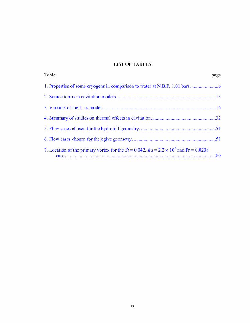
LIST OF TABLES
Table page 1. Properties of some cryogens in comparison to water at N.B.P, 1.01 bars .......................6
2. Source terms in cavitation models .................................................................................13
3. Variants of the k - ε model.............................................................................................16
4. Summary of studies on thermal effects in cavitation.....................................................32
5. Flow cases chosen for the hydrofoil geometry. .............................................................51
6. Flow cases chosen for the ogive geometry. ...................................................................51
7. Location of the primary vortex for the St = 0.042, Ra = 2.2 × 10⁵ and Pr = 0.0208 case ...........................................................................................................................80
x
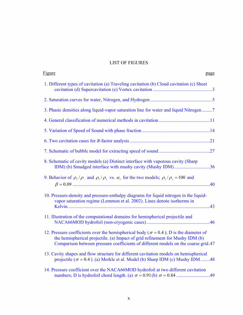
LIST OF FIGURES
Figure page 1. Different types of cavitation (a) Traveling cavitation (b) Cloud cavitation (c) Sheet
cavitation (d) Supercavitation (e) Vortex cavitation ..................................................3
2. Saturation curves for water, Nitrogen, and Hydrogen ....................................................5
3. Phasic densities along liquid-vapor saturation line for water and liquid Nitrogen.........7
4. General classification of numerical methods in cavitation ...........................................11
5. Variation of Speed of Sound with phase fraction .........................................................14
6. Two cavitation cases for B-factor analysis ...................................................................21
7. Schematic of bubble model for extracting speed of sound ...........................................27
8. Schematic of cavity models (a) Distinct interface with vaporous cavity (Sharp IDM) (b) Smudged interface with mushy cavity (Mushy IDM)..............................36
9. Behavior of /lρ ρ− and /lρ ρ+ vs. lα for the two models; / 100l vρ ρ = and 0.09β = ...................................................................................................................40
10. Pressure-density and pressure-enthalpy diagrams for liquid nitrogen in the liquid-vapor saturation regime (Lemmon et al. 2002). Lines denote isotherms in Kelvin. ......................................................................................................................43
11. Illustration of the computational domains for hemispherical projectile and NACA66MOD hydrofoil (non-cryogenic cases) .....................................................46
12. Pressure coefficients over the hemispherical body ( 0.4σ = ); D is the diameter of the hemispherical projectile. (a) Impact of grid refinement for Mushy IDM (b) Comparison between pressure coefficients of different models on the coarse grid.47
13. Cavity shapes and flow structure for different cavitation models on hemispherical projectile ( 0.4σ = ). (a) Merkle et al. Model (b) Sharp IDM (c) Mushy IDM........48
14. Pressure coefficient over the NACA66MOD hydrofoil at two different cavitation numbers; D is hydrofoil chord length. (a) 0.91σ = (b) 0.84σ = ............................49
xi
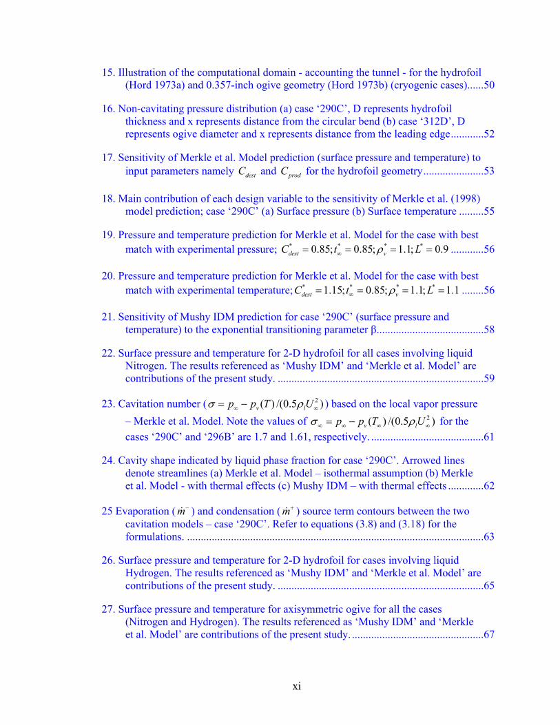
15. Illustration of the computational domain - accounting the tunnel - for the hydrofoil (Hord 1973a) and 0.357-inch ogive geometry (Hord 1973b) (cryogenic cases)......50
16. Non-cavitating pressure distribution (a) case ‘290C’, D represents hydrofoil thickness and x represents distance from the circular bend (b) case ‘312D’, D represents ogive diameter and x represents distance from the leading edge............52
17. Sensitivity of Merkle et al. Model prediction (surface pressure and temperature) to input parameters namely destC and prodC for the hydrofoil geometry......................53
18. Main contribution of each design variable to the sensitivity of Merkle et al. (1998) model prediction; case ‘290C’ (a) Surface pressure (b) Surface temperature .........55
19. Pressure and temperature prediction for Merkle et al. Model for the case with best match with experimental pressure; * * * *0.85; 0.85; 1.1; 0.9dest vC t Lρ∞= = = = ............56
20. Pressure and temperature prediction for Merkle et al. Model for the case with best match with experimental temperature; * * * *1.15; 0.85; 1.1; 1.1dest vC t Lρ∞= = = = ........56
21. Sensitivity of Mushy IDM prediction for case ‘290C’ (surface pressure and temperature) to the exponential transitioning parameter β.......................................58
22. Surface pressure and temperature for 2-D hydrofoil for all cases involving liquid Nitrogen. The results referenced as ‘Mushy IDM’ and ‘Merkle et al. Model’ are contributions of the present study. ...........................................................................59
23. Cavitation number ( 2( ) /(0.5 )v lp p T Uσ ρ∞ ∞= − ) based on the local vapor pressure – Merkle et al. Model. Note the values of 2( ) /(0.5 )v lp p T Uσ ρ∞ ∞ ∞ ∞= − for the cases ‘290C’ and ‘296B’ are 1.7 and 1.61, respectively. .........................................61
24. Cavity shape indicated by liquid phase fraction for case ‘290C’. Arrowed lines denote streamlines (a) Merkle et al. Model – isothermal assumption (b) Merkle et al. Model - with thermal effects (c) Mushy IDM – with thermal effects .............62
25 Evaporation ( m−& ) and condensation ( m+& ) source term contours between the two cavitation models – case ‘290C’. Refer to equations (3.8) and (3.18) for the formulations. ............................................................................................................63
26. Surface pressure and temperature for 2-D hydrofoil for cases involving liquid Hydrogen. The results referenced as ‘Mushy IDM’ and ‘Merkle et al. Model’ are contributions of the present study. ...........................................................................65
27. Surface pressure and temperature for axisymmetric ogive for all the cases (Nitrogen and Hydrogen). The results referenced as ‘Mushy IDM’ and ‘Merkle et al. Model’ are contributions of the present study. ................................................67
xii
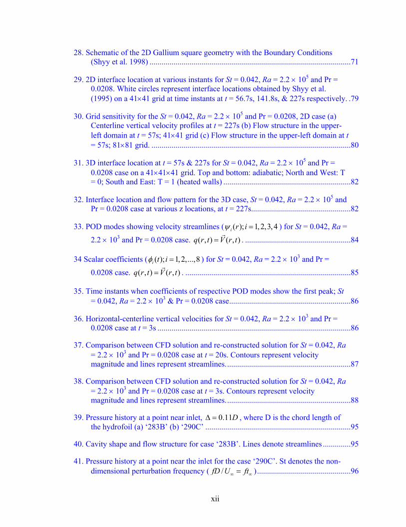
28. Schematic of the 2D Gallium square geometry with the Boundary Conditions (Shyy et al. 1998) .....................................................................................................71
29. 2D interface location at various instants for St = 0.042, Ra = 2.2 × 10⁵ and Pr = 0.0208. White circles represent interface locations obtained by Shyy et al. (1995) on a 41×41 grid at time instants at t = 56.7s, 141.8s, & 227s respectively. .79
30. Grid sensitivity for the St = 0.042, Ra = 2.2 × 10⁵ and Pr = 0.0208, 2D case (a) Centerline vertical velocity profiles at t = 227s (b) Flow structure in the upper-left domain at t = 57s; 41×41 grid (c) Flow structure in the upper-left domain at t = 57s; 81×81 grid. ....................................................................................................80
31. 3D interface location at t = 57s & 227s for St = 0.042, Ra = 2.2 × 10⁵ and Pr = 0.0208 case on a 41×41×41 grid. Top and bottom: adiabatic; North and West: T = 0; South and East: T = 1 (heated walls) ................................................................82
32. Interface location and flow pattern for the 3D case, St = 0.042, Ra = 2.2 × 10⁵ and Pr = 0.0208 case at various z locations, at t = 227s..................................................82
33. POD modes showing velocity streamlines ( ( ); 1,2,3,4i r iψ = ) for St = 0.042, Ra =
2.2 × 10³ and Pr = 0.0208 case. ( , ) ( , )q r t V r t=r
. .....................................................84
34 Scalar coefficients ( ( ); 1,2,...,8i t iφ = ) for St = 0.042, Ra = 2.2 × 10³ and Pr =
0.0208 case. ( , ) ( , )q r t V r t=r
. ...................................................................................85
35. Time instants when coefficients of respective POD modes show the first peak; St = 0.042, Ra = 2.2 × 10³ & Pr = 0.0208 case.............................................................86
36. Horizontal-centerline vertical velocities for St = 0.042, Ra = 2.2 × 10³ and Pr = 0.0208 case at t = 3s .................................................................................................86
37. Comparison between CFD solution and re-constructed solution for St = 0.042, Ra = 2.2 × 10³ and Pr = 0.0208 case at t = 20s. Contours represent velocity magnitude and lines represent streamlines...............................................................87
38. Comparison between CFD solution and re-constructed solution for St = 0.042, Ra = 2.2 × 10³ and Pr = 0.0208 case at t = 3s. Contours represent velocity magnitude and lines represent streamlines...............................................................88
39. Pressure history at a point near inlet, 0.11D∆ = , where D is the chord length of the hydrofoil (a) ‘283B’ (b) ‘290C’ .........................................................................95
40. Cavity shape and flow structure for case ‘283B’. Lines denote streamlines ..............95
41. Pressure history at a point near the inlet for the case ‘290C’. St denotes the non-dimensional perturbation frequency ( /fD U ft∞ ∞= )...............................................96
xiii
42. Pressure history at a point near the inlet for the cases ‘296B’ and ‘290C’. The non-dimensional perturbation frequency ( /fD U ft∞ ∞= ) is 1.0..............................97
43 POD modes for the velocity field; ( ); 1,2,3i r iψ = ; ( , ) ( , )q r t V r t=r
...........................98
44 POD modes for the velocity field; ( ); 1,2,3i r iψ = ; ( , ) ( , )q r t V r t=r
...........................98
xiv
LIST OF SYMBOLS
:σ cavitation number
:δ boundary layer/cavity thickness
L: length (of cavity or cavitating object)
q: heat flux; generalized flow variable in POD representation
V: total volume
t: time
x, y, z: coordinate axes
r: position vector
:ξ streamwise direction in the curvilinear co-ordinate system
i, j, k, n: indices
, , :u v w velocity components
p: pressure
T: temperature
:ρ density
:α volume fraction
f: mass fraction
h: sensible enthalpy
s: entropy

xv
c: speed of sound
:γ ratio of the two specific heats for gases
:τ stress tensor
P: production of turbulent energy
1 2, , , , , :kC C C Cε ε ε µσ σ constants
Q: total kinetic energy (inclusive of turbulent fluctuations)
k: turbulent kinetic energy
ε : turbulent dissipation
F: filter function for filter-based modeling
µ : dynamic viscosity
K: thermal conductivity
:υ volume flow rate
L: latent heat
:PC specific heat
:pC pressure coefficient
a: thermal diffusivity
m& : volume conversion rate
B: B-factor to gauge thermal effect
:Σ dimensional parameter to assess thermal effect
:β control parameter in the Mushy IDM; coefficient of thermal expansion
g: gravitational acceleration
U: velocity scale
D: length scale (such as hydrofoil chord length or ogive diameter)

xvi
R: bubble radius
CFL: Courant, Freidricks, and Levy Number
St: Stefan Number
Ra: Rayleigh Number
Pr: Prandtl Number
Re: Reynolds Number
:∆ difference; filter size in filter-based turbulence modeling
∇ : gradient or divergence operator
:ψ POD mode
:φ time-dependent coefficient in the POD series
:η energy content in the respective POD mode
Subscripts:
:∞ reference value (typically inlet conditions at the tunnel)
0: initial conditions
s: solid
l: liquid
v: vapor
m: mixture
f: friction
Q: discharge
c: cavity
L: laminar
t: turbulent
xvii
I: interfacial
n: normal to local gradient of phase fraction
sat: saturation conditions
dest: destruction of the phase
prod: production of the phase
+: condensation
-: evaporation
A, H, S, M, G, B: terms in a discretized equation
nb: neighboring nodes
P: at the cell of interest
Superscripts/Overhead symbols:
+: condensation
-: evaporation
‘: fluctuating component
*: normalized value; updated value in the context of PISO algorithm
→ : vector
-: average
~: Favre-averaged
n: time step level
k: iteration level
xviii
Abstract of Dissertation Presented to the Graduate School of the University of Florida in Partial Fulfillment of the Requirements for the Degree of Doctor of Philosophy
COMPUTATIONAL MODELING OF THERMODYNAMIC EFFECTS IN CRYOGENIC CAVITATION
By
Yogen Utturkar
August 2005
Chair: Wei Shyy Cochair: Nagaraj Arakere Major Department: Mechanical and Aerospace Engineering
Thermal effects substantially impact the cavitation dynamics of cryogenic fluids.
The present study strives towards developing an effective computational strategy to
simulate cryogenic cavitation aimed at liquid rocket propulsion applications. We employ
previously developed cavitation and compressibility models, and incorporate the thermal
effects via solving the enthalpy equation and dynamically updating the fluid physical
properties. The physical implications of an existing cavitation model are reexamined
from the standpoint of cryogenic fluids, to incorporate a mushy formulation, to better
reflect the observed “frosty” appearance within the cavity. Performance of the revised
cavitation model is assessed against the existing cavitation models and experimental data,
under non-cryogenic and cryogenic conditions.
Steady state computations are performed over a 2D hydrofoil and an axisymmetric
ogive by employing real fluid properties of liquid nitrogen and hydrogen. The
thermodynamic effect is demonstrated under consistent conditions via the reduction in
xix
the cavity length as the reference temperature tends towards the critical point. Justifiable
agreement between the computed surface pressure and temperature, and experimental
data is obtained. Specifically, the predictions of both the models are better; for the
pressure field than the temperature field, and for liquid nitrogen than liquid hydrogen.
Global sensitivity analysis is performed to examine the sensitivity of the computations to
changes in model parameters and uncertainties in material properties.
The pressure-based operator splitting method, PISO, is adapted towards typical
challenges in multiphase computations such as multiple, coupled, and non-linear
equations, and sudden changes in flow variables across phase boundaries. Performance of
the multiphase variant of PISO is examined firstly for the problem of gallium fusion. A
good balance between accuracy and stability is observed. Time-dependent computations
for various cases of cryogenic cavitation are further performed with the algorithm. The
results show reasonable agreement with the experimental data. Impact of the cryogenic
environment and inflow perturbations on the flow structure and instabilities is explained
via the simulated flow fields and the reduced order strategy of Proper Orthogonal
Decomposition (POD).
1
CHAPTER 1 INTRODUCTION AND RESEARCH SCOPE
The phenomenon by which a liquid forms gas-filled or vapor-filled cavities under
the effect of tensile stress produced by a pressure drop below its vapor pressure is termed
cavitation (Batchelor 1967). Cavitation is rife in fluid machinery such as inducers,
pumps, turbines, nozzles, marine propellers, hydrofoils, journal bearings, squeeze film
dampers etc. due to wide ranging pressure variations along the flow. This phenomenon is
largely undesirable due to its negative effects namely noise, vibration, material erosion
etc. Detailed description of these effects can be readily obtained from literature. It is
however noteworthy that the cavitation phenomenon is also associated with useful
applications. Besides drag reduction efforts (Lecoffre 1999), biomedical applications in
drug delivery (Ohl et al. 2003) and shock wave lithotripsy (Tanguay and Colonuis 2003),
environmental applications for decomposing organic compounds (Kakegawa and
Kawamura 2003) and water disinfection (Kalamuck et al. 2003), and manufacturing and
material processing applications (Soyama and Macodiyo 2003) are headed towards
receiving an impetus from cavitation. Comprehensive studies on variety of fluids such as
water, cryogens, and lubricants have provided significant insights on the dual impact of
cavitation. Experimental research methods including some mentioned above have relied
on shock waves (Ohl et al. 2003), acoustic waves (Chavanne et al. 2002), and laser pulses
(Sato et al. 1996), in addition to hydrodynamic pressure changes, for triggering
cavitation. Clearly, research potential in terms of understanding the mechanisms and
characteristics of cavitation in different fluids, and their applications and innovation is
2
tremendous. The applicability and contributions of the present study within the above-
mentioned framework are described later in this chapter.
1.1 Types of Cavitation
Different types of cavitation are observed depending on the flow conditions and
fluid properties. Each of them has distinct characteristics as compared to others. Five
major types of cavitation have been described in literature. They are as follows:
(a) Traveling cavitation
It is characterized by individual transient cavities or bubbles that form in the liquid,
expand or shrink, and move downstream (Knapp et al. 1970). Typically, it is observed on
hydrofoils at small angles of attack. The density of nuclei present in the upstream flow
highly affects the geometries of the bubbles (Lecoffre 1999). Traveling cavitation is
illustrated in Figure 1(a).
(b) Cloud cavitation
It is produced by vortex shedding in the flow field and is associated with strong
vibration, noise, and erosion (Kawanami et al. 1997). A re-entrant jet is usually the
causative mechanism for this type of cavitation (Figure 1(b)).
(c) Sheet cavitation
It is also known as fixed, attached cavity, or pocket cavitation (Figure 1(c)). Sheet
cavitation is stable in quasi-steady sense (Knapp et al. 1970). Though the liquid-vapor
interface is dependent on the nature of flow, the closure region is usually characterized by
sharp density gradients and bubble clusters (Gopalan and Katz 2000).
(d) Supercavitation
Supercavitation can be considered as an extremity of sheet cavitation wherein a
substantial fraction of the body surface is engulfed by the cavity (Figure 1(d)). It is
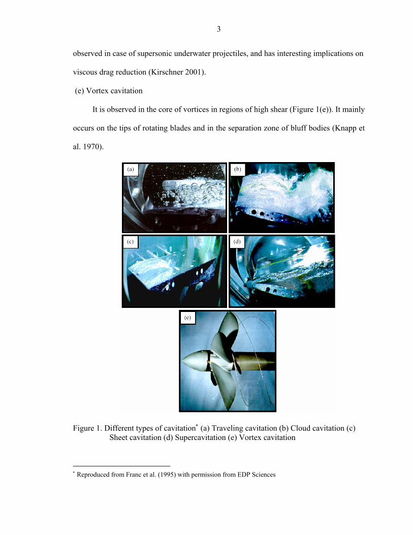
3
observed in case of supersonic underwater projectiles, and has interesting implications on
viscous drag reduction (Kirschner 2001).
(e) Vortex cavitation
It is observed in the core of vortices in regions of high shear (Figure 1(e)). It mainly
occurs on the tips of rotating blades and in the separation zone of bluff bodies (Knapp et
al. 1970).
Figure 1. Different types of cavitation∗ (a) Traveling cavitation (b) Cloud cavitation (c) Sheet cavitation (d) Supercavitation (e) Vortex cavitation
∗ Reproduced from Franc et al. (1995) with permission from EDP Sciences

4
1.2 Cavitation in Cryogenic Fluids – Thermal Effect
Cryogens serve as popular fuels for the commercial launch vehicles while
petroleum, hypergolic propellants, and solids are other options. Typically, a combination
of liquid oxygen (LOX) and liquid hydrogen (LH2) is used as rocket propellant mixture.
The boiling points of LOX and LH2 under standard conditions are -183 F and -423 F,
respectively. By cooling and compressing these gases from regular conditions, they are
stored into smaller storage tanks. The combustion of LOX and LH2 is clean since it
produces water vapor as a by-product. Furthermore, the power/gallon ratio of LH2 is high
as compared to other alternatives. Though storage, safety, and extreme low temperature
limits are foremost concerns for any cryogenic application, rewards of mastering the use
of cryogens as rocket propellants are substantial (NASA Online Facts 1991).
A turbopump is employed to supply the low temperature propellants to the
combustion chamber which is under extremely high pressure. An inducer is attached to
the turbopump to increase its efficiency. Design of any space vehicle component is
always guided by minimum size and weight criteria. Consequently, the size constraint on
the turbopump solicits high impellor speeds. Such high speeds likely result in a zone of
negative static pressure (pressure drop below vapor pressure) causing the propellant to
cavitate around the inducer blades (Tokumasu et al. 2002). In view of the dire
consequences, investigation of cavitation characteristics in cryogens, specifically LOX
and LH2, is an imperative task.
Intuitively, physical and thermal properties of a fluid are expected to significantly
affect the nature of cavitation. For example, Helium-4 shows anomalous cavitation
properties especially past the λ-point temperature mainly due to its transition to
superfluidity (Daney 1988). Besides, quantum tunneling also attributes to cavity
5
formation in Helium-4 (Lambare et al. 1998). Cavitation of Helium-4 in the presence of a
glass plate (heterogenous cavitation) has lately produced some unexpected results
(Chavanne et al. 2002), which are in contrast to its regular cavitating pattern observed
under homogenous conditions (without a foreign body). Undoubtedly, a multitude of
characteristics and research avenues are offered by different types of cryogenic fluids.
The focus of the current study is, however, restricted to cryogenic fluids such as LOX,
LH2, and liquid Nitrogen due to their aforesaid strong relevance in space applications. It
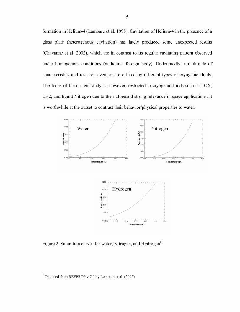
is worthwhile at the outset to contrast their behavior/physical properties to water.
Figure 2. Saturation curves for water, Nitrogen, and Hydrogen£
£ Obtained from REFPROP v 7.0 by Lemmon et al. (2002)
Water Nitrogen
Hydrogen
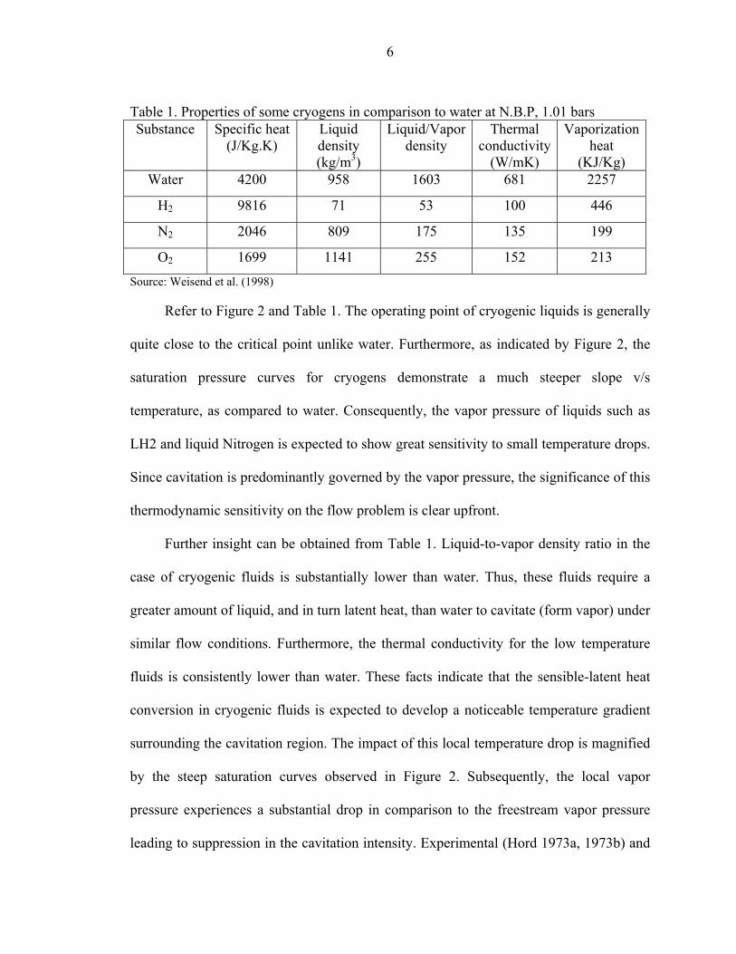
6
Table 1. Properties of some cryogens in comparison to water at N.B.P, 1.01 bars Substance Specific heat
(J/Kg.K) Liquid density (kg/m3)
Liquid/Vapor density
Thermal conductivity
(W/mK)
Vaporization heat
(KJ/Kg) Water 4200 958 1603 681 2257
H2 9816 71 53 100 446
N2 2046 809 175 135 199
O2 1699 1141 255 152 213 Source: Weisend et al. (1998)
Refer to Figure 2 and Table 1. The operating point of cryogenic liquids is generally
quite close to the critical point unlike water. Furthermore, as indicated by Figure 2, the
saturation pressure curves for cryogens demonstrate a much steeper slope v/s
temperature, as compared to water. Consequently, the vapor pressure of liquids such as
LH2 and liquid Nitrogen is expected to show great sensitivity to small temperature drops.
Since cavitation is predominantly governed by the vapor pressure, the significance of this
thermodynamic sensitivity on the flow problem is clear upfront.
Further insight can be obtained from Table 1. Liquid-to-vapor density ratio in the
case of cryogenic fluids is substantially lower than water. Thus, these fluids require a
greater amount of liquid, and in turn latent heat, than water to cavitate (form vapor) under
similar flow conditions. Furthermore, the thermal conductivity for the low temperature
fluids is consistently lower than water. These facts indicate that the sensible-latent heat
conversion in cryogenic fluids is expected to develop a noticeable temperature gradient
surrounding the cavitation region. The impact of this local temperature drop is magnified
by the steep saturation curves observed in Figure 2. Subsequently, the local vapor
pressure experiences a substantial drop in comparison to the freestream vapor pressure
leading to suppression in the cavitation intensity. Experimental (Hord 1973a, 1973b) and

7
numerical results (Deshpande et al. 1997) on sheet cavitation have shown a 20-40%
reduction in cavity length due to the thermodynamic effects in cryogenic fluids.
Figure 3. Phasic densities along liquid-vapor saturation line for water and liquid
Nitrogen¥
Additionally, the physical properties of cryogenic fluids, other than vapor pressure, are
also thermo-sensible, as illustrated in Figure 3. Thus, from a standpoint of numerical
computations, simulating cryogenic cavitation implies a tight coupling between the non-
linear energy equation, momentum equations, and the cavitation model, via the iterative
update of fluid properties (such as vapor pressure, densities, specific heat, thermal
conductivity, viscosity etc.) with changes in the local temperature. Encountering these
difficulties is expected to yield a numerical methodology specifically well-suited for
cryogenic cavitation, and forms the key emphasis of the present study.
¥ Obtained from REFPROP v 7.0 by Lemmon et al. (2002)
Water Liq. N2
8
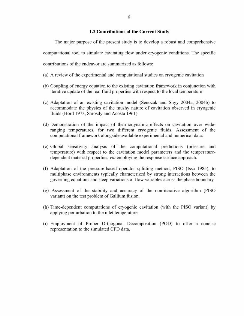
1.3 Contributions of the Current Study
The major purpose of the present study is to develop a robust and comprehensive
computational tool to simulate cavitating flow under cryogenic conditions. The specific
contributions of the endeavor are summarized as follows:
(a) A review of the experimental and computational studies on cryogenic cavitation (b) Coupling of energy equation to the existing cavitation framework in conjunction with
iterative update of the real fluid properties with respect to the local temperature (c) Adaptation of an existing cavitation model (Senocak and Shyy 2004a, 2004b) to
accommodate the physics of the mushy nature of cavitation observed in cryogenic fluids (Hord 1973, Sarosdy and Acosta 1961)
(d) Demonstration of the impact of thermodynamic effects on cavitation over wide-
ranging temperatures, for two different cryogenic fluids. Assessment of the computational framework alongside available experimental and numerical data.
(e) Global sensitivity analysis of the computational predictions (pressure and
temperature) with respect to the cavitation model parameters and the temperature-dependent material properties, via employing the response surface approach.
(f) Adaptation of the pressure-based operator splitting method, PISO (Issa 1985), to
multiphase environments typically characterized by strong interactions between the governing equations and steep variations of flow variables across the phase boundary
(g) Assessment of the stability and accuracy of the non-iterative algorithm (PISO
variant) on the test problem of Gallium fusion. (h) Time-dependent computations of cryogenic cavitation (with the PISO variant) by
applying perturbation to the inlet temperature (i) Employment of Proper Orthogonal Decomposition (POD) to offer a concise
representation to the simulated CFD data.
9
CHAPTER 2 LITERATURE REVIEW
Cavitation has been the focal point of numerous experimental and numerical
studies in the area of fluid dynamics. A review of these studies is presented in this
chapter. Since cryogenic cavitation remains the primary interest of this study, the general
review on cavitation studies is purely restricted according to relevance. Specifically, the
numerical approaches in terms of cavitation, compressibility, and turbulence modeling
are briefly reviewed in the earlier section with reference to pertinent experiments. The
later section mainly delves into the issues of thermal effects of cavitation. Current status
of numerical strategies in modeling cryogenic cavitation, and their merits and limitations
are reported to underscore the gap bridged by the current research study.
2.1 General Review of Recent Studies
Computational modeling of cavitation has complemented experimental research on
this topic for a long time. Some earlier studies (Reboud et al. 1990, Deshpande et al.
1994) relied on potential flow assumption (Euler equations) to simulate flow around the
cavitating body. However, simulation strategies by solving the Navier-Stokes equations
have gained momentum only in the last decade. Studies in this regard can be broadly
classified based on their interface capturing method. Chen and Heister (1996) and
Deshpande et al. (1997) adopted the interface tracking Marker and Cell approach in their
respective studies, which were characterized by time-wise grid regeneration and the
constant cavity-pressure assumption. The liquid-vapor interface in these studies was
explicitly updated at each time step by monitoring the surface pressure, followed by its
10
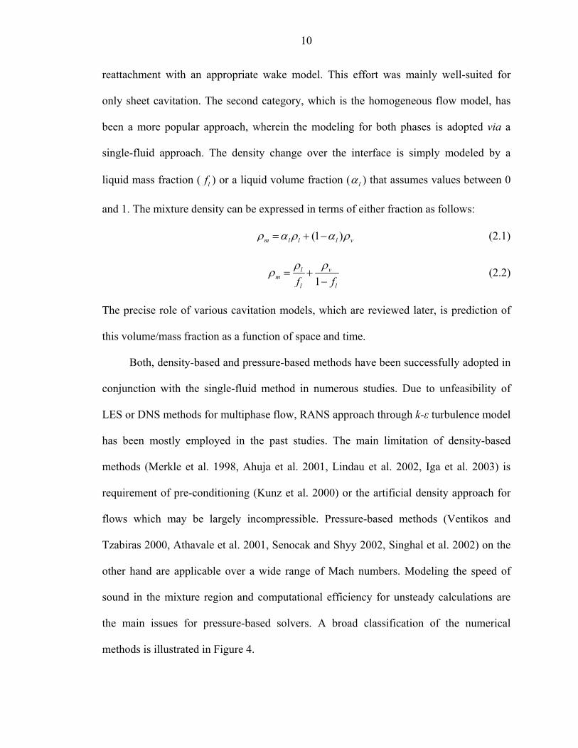
reattachment with an appropriate wake model. This effort was mainly well-suited for
only sheet cavitation. The second category, which is the homogeneous flow model, has
been a more popular approach, wherein the modeling for both phases is adopted via a
single-fluid approach. The density change over the interface is simply modeled by a
liquid mass fraction ( lf ) or a liquid volume fraction ( lα ) that assumes values between 0
and 1. The mixture density can be expressed in terms of either fraction as follows:
(1 )m l l l vρ α ρ α ρ= + − (2.1)
1l v
ml lf fρ ρρ = +
− (2.2)
The precise role of various cavitation models, which are reviewed later, is prediction of
this volume/mass fraction as a function of space and time.
Both, density-based and pressure-based methods have been successfully adopted in
conjunction with the single-fluid method in numerous studies. Due to unfeasibility of
LES or DNS methods for multiphase flow, RANS approach through k-ε turbulence model
has been mostly employed in the past studies. The main limitation of density-based
methods (Merkle et al. 1998, Ahuja et al. 2001, Lindau et al. 2002, Iga et al. 2003) is
requirement of pre-conditioning (Kunz et al. 2000) or the artificial density approach for
flows which may be largely incompressible. Pressure-based methods (Ventikos and
Tzabiras 2000, Athavale et al. 2001, Senocak and Shyy 2002, Singhal et al. 2002) on the
other hand are applicable over a wide range of Mach numbers. Modeling the speed of
sound in the mixture region and computational efficiency for unsteady calculations are
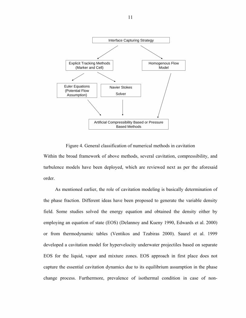
the main issues for pressure-based solvers. A broad classification of the numerical
methods is illustrated in Figure 4.
11
Interface Capturing Strategy
Explicit Tracking Methods (Marker and Cell)
Homogenous Flow Model
Euler Equations (Potential Flow Assumption)
Navier Stokes
Solver
Artificial Compressibility Based or Pressure Based Methods
Figure 4. General classification of numerical methods in cavitation
Within the broad framework of above methods, several cavitation, compressibility, and
turbulence models have been deployed, which are reviewed next as per the aforesaid
order.
As mentioned earlier, the role of cavitation modeling is basically determination of
the phase fraction. Different ideas have been proposed to generate the variable density
field. Some studies solved the energy equation and obtained the density either by
employing an equation of state (EOS) (Delannoy and Kueny 1990, Edwards et al. 2000)
or from thermodynamic tables (Ventikos and Tzabiras 2000). Saurel et al. 1999
developed a cavitation model for hypervelocity underwater projectiles based on separate
EOS for the liquid, vapor and mixture zones. EOS approach in first place does not
capture the essential cavitation dynamics due to its equilibrium assumption in the phase
change process. Furthermore, prevalence of isothermal condition in case of non-
12
thermosensible fluids such as water imparts a barotropic form, ( )m f pρ = , to the EOS.
Thus, cavitation modeling via employing the EOS is devoid of the capability to capture
barotropic vorticity generation in the wake region as demonstrated by Gopalan and Katz
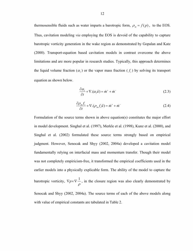
(2000). Transport-equation based cavitation models in contrast overcome the above
limitations and are more popular in research studies. Typically, this approach determines
the liquid volume fraction ( lα ) or the vapor mass fraction ( vf ) by solving its transport
equation as shown below.
.( )llu m m
tα α + −∂
+∇ = +∂
r& & (2.3)
.( )m vm v
f f u m mt
ρ ρ + −∂+∇ = +
∂r
& & (2.4)
Formulation of the source terms shown in above equation(s) constitutes the major effort
in model development. Singhal et al. (1997), Merkle et al. (1998), Kunz et al. (2000), and
Singhal et al. (2002) formulated these source terms strongly based on empirical
judgment. However, Senocak and Shyy (2002, 2004a) developed a cavitation model
fundamentally relying on interfacial mass and momentum transfer. Though their model
was not completely empiricism-free, it transformed the empirical coefficients used in the
earlier models into a physically explicable form. The ability of the model to capture the
barotropic vorticity, 1pρ
∇ ×∇ , in the closure region was also clearly demonstrated by
Senocak and Shyy (2002, 2004a). The source terms of each of the above models along
with value of empirical constants are tabulated in Table 2.
13
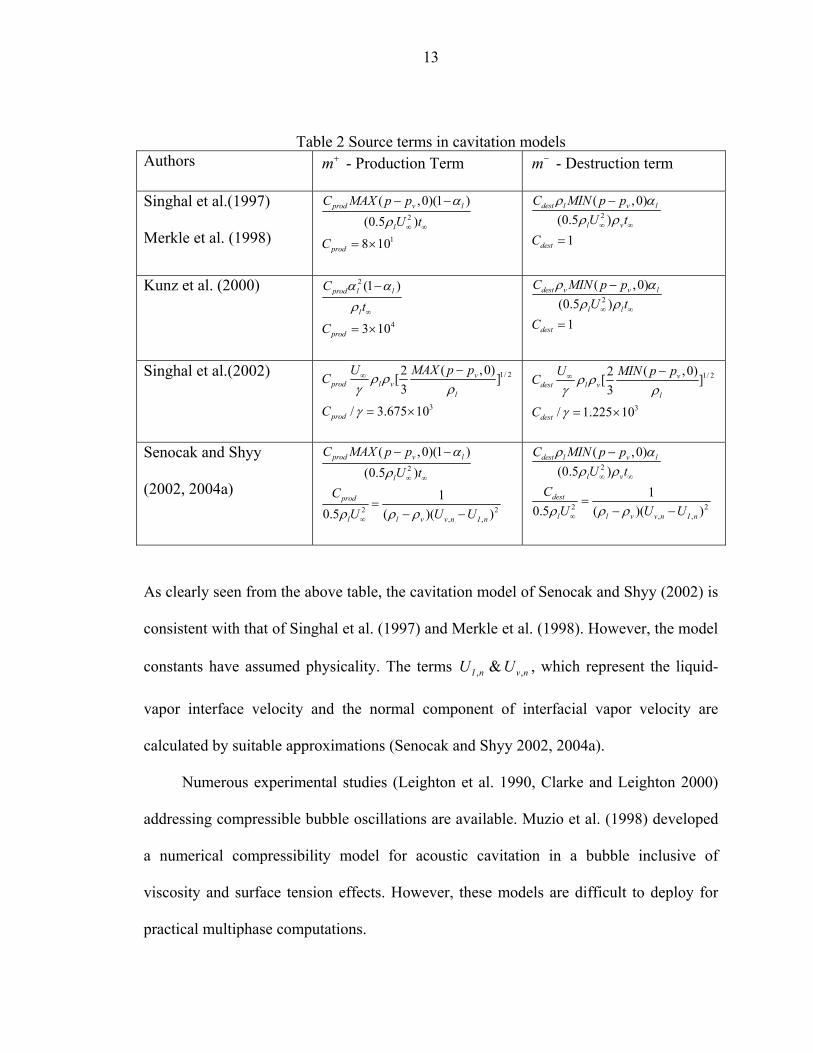
Table 2 Source terms in cavitation models Authors m+ - Production Term m− - Destruction term
Singhal et al.(1997)
Merkle et al. (1998) 2
1
( ,0)(1 )(0.5 )
8 10
prod v l
l
prod
C MAX p pU t
C
αρ ∞ ∞
− −
= ×
2
( ,0)(0.5 )
1
dest l v l
l v
dest
C MIN p pU t
C
ρ αρ ρ∞ ∞
−
=
Kunz et al. (2000) 2
4
(1 )
3 10
prod l l
l
prod
Ct
C
α αρ ∞
−
= ×
2
( ,0)(0.5 )
1
dest v v l
l l
dest
C MIN p pU t
C
ρ αρ ρ∞ ∞
−
=
Singhal et al.(2002) 1/ 2
3
( ,0)2[ ]3
/ 3.675 10
vprod l v
l
prod
MAX p pUC
C
ρ ργ ρ
γ
∞ −
= ×
1/ 2
3
( ,0)2[ ]3
/ 1.225 10
vdest l v
l
dest
MIN p pUC
C
ρ ργ ρ
γ
∞ −
= ×
Senocak and Shyy
(2002, 2004a) 2
2 2, ,
( ,0)(1 )(0.5 )
10.5 ( )( )
prod v l
l
prod
l l v v n I n
C MAX p pU t
CU U U
αρ
ρ ρ ρ
∞ ∞
∞
− −
=− −
2
2 2, ,
( ,0)(0.5 )
10.5 ( )( )
dest l v l
l v
dest
l l v v n I n
C MIN p pU t
CU U U
ρ αρ ρ
ρ ρ ρ
∞ ∞
∞
−
=− −
As clearly seen from the above table, the cavitation model of Senocak and Shyy (2002) is
consistent with that of Singhal et al. (1997) and Merkle et al. (1998). However, the model
constants have assumed physicality. The terms , ,&I n v nU U , which represent the liquid-
vapor interface velocity and the normal component of interfacial vapor velocity are
calculated by suitable approximations (Senocak and Shyy 2002, 2004a).
Numerous experimental studies (Leighton et al. 1990, Clarke and Leighton 2000)
addressing compressible bubble oscillations are available. Muzio et al. (1998) developed
a numerical compressibility model for acoustic cavitation in a bubble inclusive of
viscosity and surface tension effects. However, these models are difficult to deploy for
practical multiphase computations.
14
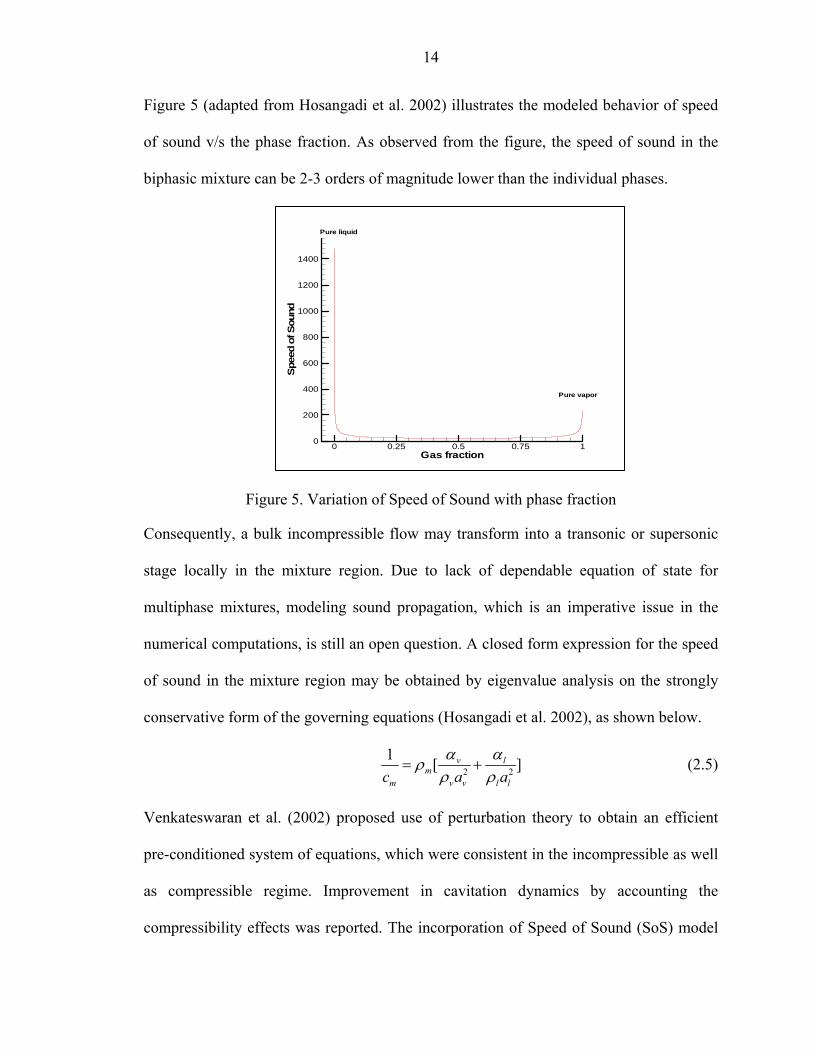
Figure 5 (adapted from Hosangadi et al. 2002) illustrates the modeled behavior of speed
of sound v/s the phase fraction. As observed from the figure, the speed of sound in the
biphasic mixture can be 2-3 orders of magnitude lower than the individual phases.
Figure 5. Variation of Speed of Sound with phase fraction
Consequently, a bulk incompressible flow may transform into a transonic or supersonic
stage locally in the mixture region. Due to lack of dependable equation of state for
multiphase mixtures, modeling sound propagation, which is an imperative issue in the
numerical computations, is still an open question. A closed form expression for the speed
of sound in the mixture region may be obtained by eigenvalue analysis on the strongly
conservative form of the governing equations (Hosangadi et al. 2002), as shown below.
2 2
1 [ ]v lm
m v v l lc a aα αρρ ρ
= + (2.5)
Venkateswaran et al. (2002) proposed use of perturbation theory to obtain an efficient
pre-conditioned system of equations, which were consistent in the incompressible as well
as compressible regime. Improvement in cavitation dynamics by accounting the
compressibility effects was reported. The incorporation of Speed of Sound (SoS) model
Gas fraction
Spe
edof
Sou
nd
0 0.25 0.5 0.75 10
200
400
600
800
1000
1200
1400
Pure liquid
Pure vapor
15
into pressure-based cavitation computations was significantly advanced by Senocak and
Shyy (2002, 2003). In pressure-based solvers, the SoS model affects the solution mainly
through the pressure correction equation. The following relationship is adopted between
the density correction and the pressure correction terms, while enforcing the mass-
conservation treatment through the pressure correction equation:
' 'm C pρρ = (2.6)
The implementation of equation (2.6) imparts a convective-diffusive form to the pressure
equation. Two SoS models were proposed by Senocak and Shyy (2003, 2004a, 2004b).
SoS-1: ( ) (1 )s lC Cpρρ α∂
= = −∂
(2.7)
1 1
1 1
SoS-2 : ( ) ( ) i is
i i
Cp p p pρ ξ
ρ ρρ ρ + −
+ −
−∆ ∂= = =
∆ ∂ − (2.8)
While SoS-1 is a suitable approximation to the curve shown in Figure 5, SoS-2
approximates the fundamental definition of speed of sound by adopting a central-
difference spatial derivative along the streamline direction (ξ) instead of differentiating
along the isentropic curve. Computations by Senocak and Shyy (2003) on convergent-
divergent nozzle demonstrated far better capability of SoS-2 to mimic the transient
behavior observed in experiments. Wu et al. (2003b) extended the model assessment by
pointing out the dramatic time scale differences between the two models. This points the
fact that compressibility modeling is a sensitivity issue and must be handled carefully.
RANS-based approaches in form of two-equation k - ε models have been actively
pursued to model turbulent cavitating flows. The k and ε transport equations along with
the definition of turbulent viscosity are summarized below.
16
( )( ) P [( ) ]m jm tt m
j j k j
u kk kt x x x
ρρ µρ ε µσ
∂∂ ∂ ∂+ = − + +∂ ∂ ∂ ∂
% (2.9)
2
1 1
( )( ) P [( ) ]m jm tt m
j j j
uC C
t x k k x xε εε
ρ ερ ε µε ε ερ µσ
∂∂ ∂ ∂+ = − + +∂ ∂ ∂ ∂
% (2.10)
The production of turbulent kinetic energy (Pt) is defined as:
P R it ij
j
ux
τ ∂=
∂%
(2.11)
while, the turbulent viscosity is defined as: 2
mt
C kµρµ
ε= (2.12)
The model coefficients, namely, 1 2, , and kC Cε ε εσ σ have three known non-trivial variants which have been summarized in Table 3.
Table 3. Variants of the k - ε model Authors 1Cε and Relevant Details 2Cε kσ εσ
Launder and
Spalding (1974)
1.44 1.92 1.3 1.0
Shyy et al. (1997) P1.15 0.25 t
ε+ ⋅ 1.9 1.15 0.89
Younis (2003)
(personal
communication)
P(1.15 0.25 ) (1 0.38 | | / )t k Q Q
tε ε∂
+ × + ⋅ ⋅∂
where 2/)( 222 wvukQ +++=
1.9 1.15 0.89
Johansen et al.
(2004)
1.44
2
, 0.09mt
C kF Cµ
µ
ρµ
ε= = , 3/ 2Min[1, ]F C
kε
∆
∆=
1.92 1.3 1.0
While the Launder and Spalding (1974) model is calibrated for equilibrium shear flows,
the model by Shyy et al. (1997) accommodates non-equilibrium effects by introducing a

17
subtle turbulent time scale into 1Cε . The RANS model of Younis (2003, personal
communication), in comparison, accounts for the time history effects of the flow. Wu et
al. (2003a, 2003b) assessed the above RANS models on turbulent cavitating flow in a
valve. Experimental visuals of the valve flow (Wang 1999) have demonstrated cavitation
instability in form of periodic cavity detachment and shedding. However, Wu et al.
(2003b) reported that the k - ε model over predicts the turbulent viscosity and damps such
instabilities. Consequently, the RANS computations were unable to capture the shedding
phenomenon, and also showed restrained sensitivity to the above variants of the k - ε
model. From standpoint of an alternate approach, the impact of filter-based turbulence
modeling on cavitating flow around a hydrofoil was reported (Wu et al. 2003c). The
filter-based model relies on the two-equation formulation and uses identical coefficient
values as proposed by Launder and Spalding (1974), but imposes a filter on the turbulent
viscosity as seen below.
2
, 0.09mt
C kF Cµ
µ
ρµ
ε= = (2.13)
The filter function (F) is defined in terms of filter size (∆ ) as:
3/ 2Min[1, ]; 1F C Ckε
∆ ∆
∆= = (2.14)
Note that the forms of viscosity in equations (2.12) and (2.13) are comparable barring the
filter function. The proposed model recovers the Launder and Spalding (1974) model for
coarse filter sizes. Furthermore, at near-wall regions, the imposed filter value F = 1
enables the use of wall functions to model the shear layer. However, in the far field zone
if the filter size is able address the turbulent length scale 3/ 2kε
, the solution is computed
18
directly ( 0tµ ≈ ). The filter-based model is also characterized by the independence of the
filter size from the grid size. This model enhanced the prediction of flow structure for
single-phase flow across a solid cylinder (Johansen et al. 2004). Wu et al. (2003c)
reported substantial unsteady characteristics for cavitating flow around a hydrofoil
because of this newly developed model. Furthermore, the time-averaged results of Wu et
al. (2003c) (surface pressure, cavity morphology, lift, drag etc.) are consistent to those
obtained by alternate studies (Kunz et al. 2003, Coutier-Delgosha et al. 2003, Qin et al.
2003). Further examination in the context of filter-based modeling and cavitating flows
was performed over the Clark-Y aerofoil and a convergent-divergent nozzle (Wu et al.
2004, 2005). The filter-based model produced pronounced time-dependent behavior in
either case due to significantly low levels of eddy viscosity. While the time-averaged
results showed consistency to experimental data, they were unable to capture the essence
of unsteady phenomena in the flow-field such as wave propagation. In addition to
implementing the two-equation model for turbulent viscosity, Athavale et al. (2000) also
accounted for turbulent pressure fluctuations. Thus, the threshold cavitation pressure (Pv)
was modified as:
' / 2v v tp p p= + (2.15)
The turbulent pressure fluctuations were modeled as follows:
0.39t mp kρ= (2.16)
Though their computations produced consistent results, the precise effect of incorporating
the turbulent pressure fluctuations was not discerned.
19
In addition to the above review, Wang et al. (2001), Senocak and Shyy (2002,
2004a, 2004b), Ahuja et al. (2001), Venkateswaran et al. (2002), and Preston et al. (2001)
have also reviewed the recent efforts made in computational and modeling aspects.
2.2 Modeling Thermal Effects of Cavitation
Majority of studies on cavitation have made the assumption of isothermal
conditions since they focused on water. However, as explained earlier, these assumptions
are not suitable under cryogenic conditions because of their low liquid-vapor density
ratios, low thermal conductivities, and steep slope of pressure-temperature saturation
curves. Efforts on experimental and numerical investigation of cryogenic cavitation are
dated as back as 1969. Though the number of experimental studies on this front is
restricted due to the low temperature conditions, sufficient benchmark data for the
purpose of numerical validation is available. However, there is a dearth of robust
numerical techniques to tackle this problem numerically. The following sub-sections
provide fundamental insight into the phenomenon in addition to a literature review.
2.2.1 Scaling Laws
Similarity of cavitation dynamics is dictated primarily by the cavitation number (σ)
defined as (Brennen 1994, 1995):
2
( )0.5
v
l
p p TU
σρ
∞ ∞
∞
−= (2.17)
Under cryogenic conditions, however, cavitation occurs at the local vapor pressure
dominated by the temperature depression. Thus, the cavitation number for cryogenic
fluids is modified as:
2
( )0.5
v cc
l
p p TU
σρ
∞
∞
−= (2.18)
20
where, Tc is the local temperature in the cavity. The two cavitation numbers can be
related by a first-order approximation as follows:
21 ( ) ( )2
vl c c
dpU T TdT
ρ σ σ∞ ∞− = − (2.19)
Clearly, the local temperature depression ( cT T∞− ) causes an increase in the effective
cavitation number, consequently reducing the cavitation intensity. Furthermore, equation
(2.19) underscores the effect of the steep pressure-temperature curves shown in Chapter
1.
Quantification of the temperature drop in cryogenic cavitation has been
traditionally assessed in terms of a non-dimensional temperature drop termed as B-factor
(Ruggeri and Moore 1969). A simple heat balance between the two phases can estimate
the scale of temperature difference caused by thermal effect.
v v l l PlL C Tρ υ ρυ= ∆ (2.20)
Here, vυ and lυ are volume flow rates for the vapor and liquid phase respectively. The B-
factor can then be estimated as:
** ;v v
l l Pl
LTB TT C
υ ρυ ρ
∆= = ∆ =
∆ (2.21)
Consider the following two flow scenarios for estimating B, as shown in Figure 6
(adapted from Franc et al. 2003).
21
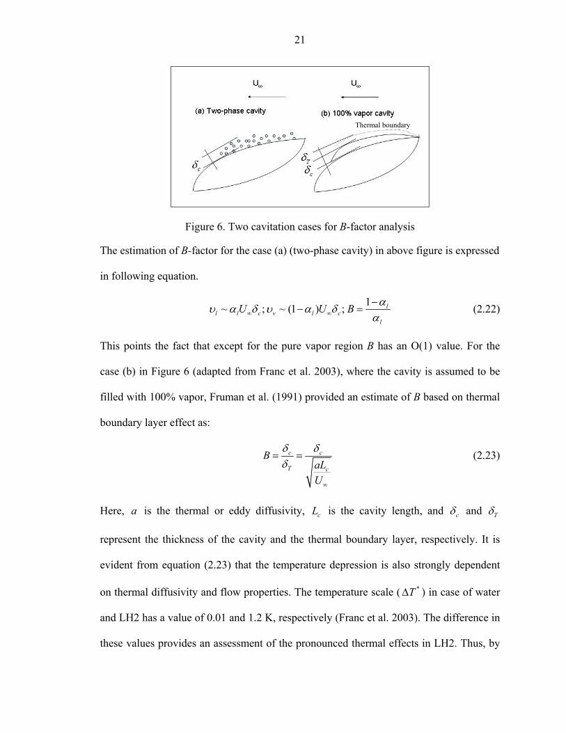
Figure 6. Two cavitation cases for B-factor analysis
The estimation of B-factor for the case (a) (two-phase cavity) in above figure is expressed
in following equation.
1~ ; ~ (1 ) ; ll l c v l c
l
U U B αυ α δ υ α δα∞ ∞
−− = (2.22)
This points the fact that except for the pure vapor region B has an O(1) value. For the
case (b) in Figure 6 (adapted from Franc et al. 2003), where the cavity is assumed to be
filled with 100% vapor, Fruman et al. (1991) provided an estimate of B based on thermal
boundary layer effect as:
c c
T c
BaLU
δ δδ
∞
= = (2.23)
Here, a is the thermal or eddy diffusivity, cL is the cavity length, and cδ and Tδ
represent the thickness of the cavity and the thermal boundary layer, respectively. It is
evident from equation (2.23) that the temperature depression is also strongly dependent
on thermal diffusivity and flow properties. The temperature scale ( *T∆ ) in case of water
and LH2 has a value of 0.01 and 1.2 K, respectively (Franc et al. 2003). The difference in
these values provides an assessment of the pronounced thermal effects in LH2. Thus, by
Thermal boundary
22
knowing the values of *T∆ and B (from equations (2.22) and (2.23)), the actual
temperature drop can be estimated. The B-factor, however, fails to consider time-
dependent or transient thermal effects due to its dependence on a steady heat balance
equation. Furthermore, the sensitivity of vapor pressure to the temperature drop, which is
largely responsible in altering cavity morphology (Deshpande et al. 1997), is not
accounted by it. As a result, though the B-factor may estimate the temperature drop
reasonably, it is inadequate to evaluate the impact of the thermal drop on the cavity
structure and the overall flow.
Brennen (1994, 1995) developed a more appropriate parameter to assess the
thermodynamic effect by incorporating it into the Rayleigh-Plesset equation
(equation(2.24)) for bubble dynamics.
22
2
3[ ( ) ] ( )2l v c
d R dRR p T pdt dt
ρ ∞+ = − (2.24)
With help of equation(2.19), we can re-write above equation as:
22
2
3[ ( ) ] ( )2
vl v
dpd R dRR T p T pdt dt dT
ρ ∞ ∞+ + ∆ = − (2.25)
From standpoint of a transiently evolving bubble, the heat flux q at any time t can be
expressed as:
Tq Kat∆
= (2.26)
The denominator in equation(2.26), at , represents the thickness of the evolving
thermal boundary layer at time t. The heat balance across the bubble interface is
expressed as follows.
2 344 [ ]3v
dq R L Rdt
π ρ π= (2.27)
23
Combining equations (2.26) and (2.27) we obtain:
v
l Pl
LR tTCaρρ
∆ ≈&
(2.28)
Introducing this temperature difference into equation(2.25) we obtain:
22
2
( )3[ ( ) ]2
v
l
p T pd R dRR R tdt dt ρ
∞ ∞−+ +Σ =& (2.29)
A close observation yields the fact that the impact of thermal effect on bubble dynamics
depends on Σ which is defined as:
2v v
l Pl
L dPdTC a
ρρ
Σ = (2.30)
The units of Σ are m/s3/2 and it proposes a criterion to determine if cavitation process is
thermally controlled or not.
Franc et al. (2003) have recently extended the above analysis to pose a criterion for
dynamic similarity between two thermally controlled cavitating flows. They replaced the
time dependency in equation(2.29) by spatial-dependency through a simple
transformation x U t∞= . Here, x is the distance traversed by a bubble in the flow-field in
time t. If D is chosen as a characteristic length scale of the problem, the Rayleigh-Plesset
equation can be recast in the following form:
23
3[ ]2 2
pCDRR R R tU
σ
∞
++ + Σ = −&& & & (2.31)
In equation (2.31), all the quantities with a bar are non-dimensional, and Cp is the
pressure coefficient. All the derivatives are with respect to /x x D= . The above equation
points out the fact that, besides σ∞ , two thermally dominated flows can be dynamically
24
similar if they have a consistent value of the non-dimensional quantity 3/D U∞Σ . It is
important to note the important role of velocity scale U∞ in the quantification of thermal
effect at this juncture. Franc et al. (2003) suggested that though thorough scaling laws for
thermosensible cavitation are difficult to develop, a rough assessment may be gained
from above equation. However, it is imperative to highlight that all the above scaling
laws have been developed using either steady-state heat balance or single bubble
dynamics. As a consequence, their applicability to general engineering environments and
complex flow cases is questionable.
The following sections will discuss the experimental and numerical investigations
of cavitation with thermal consideration. Particularly, emphasis is laid on the limitations
of currently known numerical techniques. Experimental studies are cited solely according
to their relevance to the current study.
2.2.2 Experimental Studies
Sarosdy and Acosta (1961) detected significant difference between water cavitation
and Freon cavitation. Their apparatus comprised a hydraulic loop with an investigative
window. While water cavitation was clear and more intense, they reported that cavitation
in Freon, under similar conditions, was frothy with greater entrainment rates and lower
intensity. Though their observations clearly unveiled the dominance of thermal effects in
Freon, they were not corroborated with physical understanding or numerical data. The
thermodynamic effects in cavitation were experimentally quantified as early as 1969.
Ruggeri et al. (1969) investigated methods to predict performance of pumps under
cavitating conditions for different temperatures, fluids, and operating conditions.
Typically, strategies to predict the Net Positive Suction Head (NPSH) were developed.
25
The slope of pressure-temperature saturation curve was approximated by the Clausius-
Clapeyron equation. Pump performance under various flow conditions such as discharge
coefficient and impellor frequency was assessed for variety of fluids such as water, LH2,
and butane. Hord (1973a, 1973b) published comprehensive experimental data on
cryogenic cavitation in ogives and hydrofoils. These geometries were mounted inside a
tunnel with a glass window to capture visuals of the cavitation zone. Pressure and
temperature were measured at five probe location over the geometries. Several
experiments were performed under varying inlet conditions and their results were
documented along with the instrumentation error. As a result, Hord’s data are considered
benchmark results for validating numerical techniques for thermodynamic effects in
cavitation.
From standpoint of latest investigations, Fruman et al. (1991) proposed that thermal
effect of cavitation can be estimated by attributing a rough wall behavior to the cavity
interface. Thus, heat transfer equations for a boundary layer flow over a flat plate were
applied to the problem. The volume flow rate in the cavity was estimated by producing an
air-ventilated cavity of similar shape and size. An intrinsic limitation of the above method
is its applicability to only sheet-type cavitation. Larrarte et al. (1995) used high-speed
photography and video imaging to observe natural as well as ventilated cavities on a
hydrofoil. They also examined the effect of buoyancy on interfacial stability by
conducting experiments at negative and positive AOA. They reported that vapor
production rate for a growing cavity may differ substantially from the vapor production
rate of a steady cavity. Furthermore, there may not be any vapor production during the
detachment stage of the cavity. They also noticed that cavity interface under the effect of
26
gravity may demonstrate greater stability. Fruman et al. (1999) investigated cavitation in
R-114 on a venturi section employing assumptions similar to their previous work
(Fruman et al. 1991). The temperature on the cavity surface was estimated using the
following flat plate equation.
0.1
2.1[1 (1 Pr)]0.5 Replate
l Pl f x
qT TC U Cρ∞
∞
= + − − (2.32)
Note that fC is the coefficient of friction and plateT is assumed to be equal to the local
cavity surface temperature. The heat flux q on cavity surface was estimated as:
v Qq LU Cρ ∞= − (2.33)
The discharge coefficient QC was obtained from an air-ventilated cavity of similar size.
They estimated the temperature drop via the flat plate equation and measured it
experimentally as well. These two corresponding results showed reasonable agreement.
Franc et al. (2001) employed pressure spectra to investigate R-114 cavitation on inducer
blades. The impact of thermodynamic effect was examined at three reference fluid
temperatures. They reported a delay in the onset of blade cavitation at higher reference
fluid temperatures, which was attributed to suppression of cavitation by thermal effects.
Franc et al. (2003) further investigated thermal effects in a cavitating inducer. By
employing pressure spectra they observed shift in nature of cavitation from alternate
blade cavitation to rotating cavitation with decrease in cavitation number. The earlier is
characterized by a frequency 2fb (fb is the rotor frequency with 4 blades) while the later is
characterized by a resonant frequency fb. Furthermore, R-114 was employed as the test
fluid with the view of extending its results to predicting cavitating in LH2. The scaling
27
analysis provided in section 2.2.1 was developed by Franc et al. (2003) mainly to ensure
dynamic similarity of cavitation in their experiments.
2.2.3 Numerical Modeling of Thermal Effects
Numerical modeling has been implemented in cavitation studies broadly for two
thermodynamic aspects. Firstly, attempts to model the compressible/pressure work in
bubble oscillations have been made. Lertnuwat et al. (2001) modeled bubble oscillations
by applying thermodynamic considerations to the Rayleigh-Plesset equation, and
compared the solutions to full DNS calculations. The bubble model showed good
agreement with the DNS results. The modeled behavior, however, deviated from the
DNS solutions under isothermal and adiabatic assumptions.
bubble
liquid
(1 )v vVε−
v vVε
l lVε (1 )l lVε−
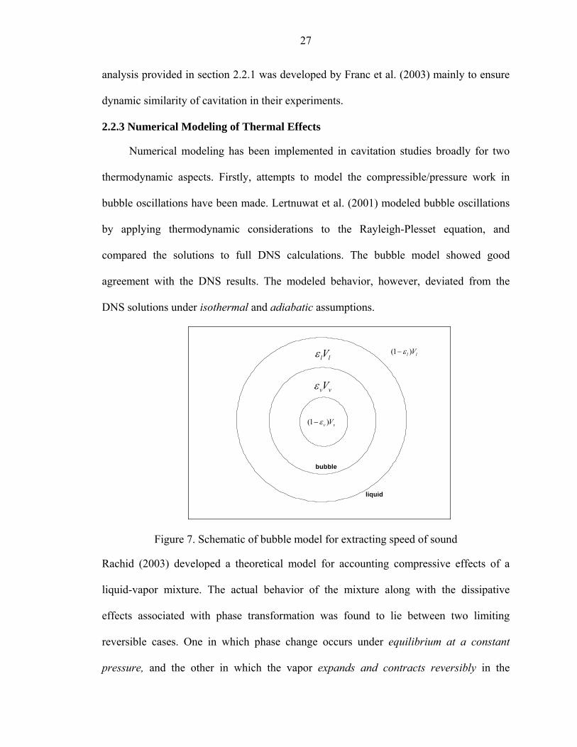
Figure 7. Schematic of bubble model for extracting speed of sound
Rachid (2003) developed a theoretical model for accounting compressive effects of a
liquid-vapor mixture. The actual behavior of the mixture along with the dissipative
effects associated with phase transformation was found to lie between two limiting
reversible cases. One in which phase change occurs under equilibrium at a constant
pressure, and the other in which the vapor expands and contracts reversibly in the
28
mixture without undergoing phase change. Rapposelli and Agostino (2003) recently
extracted the speed of sound for various fluids such as water, LOX, LH2 etc. employing a
bubble model and rigorous thermodynamic relationships. The control volume (V) of the
bubble is illustrated in Figure 7 (adapted from Rapposelli and Agostino 2003), and can be
expressed as:
(1 ) ( ) (1 ) ( )l l l l v v v vV V V V Vε ε ε ε= − + + − + (2.34)
The model assumed that thermodynamic equilibrium between the two phases is only
achieved amidst fractions lε and vε of the total volume. Subsequently, the remaining
fractions of the two phases were assumed to behave isentropically. If ml and mv are
masses associated with the respective phases, the differential volume change dV can be
expressed as:
(1 ) ( ) (1 ) ( )
( ) ( ) ( ) ( )
( )
l v
l l v vl s v s
l v
l l v vl sat v sat
l v
v l
v l
d ddVV dp dp
d ddp dp
dmm m
α ρ α ρε ερ ρ
α ρ α ρε ερ ρα α
= − − − −
− −
+ −
(2.35)
A close observation of above equation yields that the modeling extremities of
, 0 and , 1l v l vε ε ε ε= = also correspond to the thermodynamic extremities mentioned in
above-mentioned analyses by Lertnuwat et al. (2001) and Rachid (2003) (italicized in the
above description). Finally, substitution of various thermodynamic relations into equation
(2.35) yields a thermally consistent speed of sound in the medium. Rapposelli and
Agostino (2003) reported that their developed model was able to capture most features of
bubble dynamics reasonably well.
29
The second thermodynamic aspect of cavitation, which also forms the focal point
of this study, is the effect of latent heat transfer. The number of numerical studies, at least
in open literature, in this regard is highly restricted. Reboud et al. (1990) proposed a
partial cavitation model for cryogenic cavitation. The model comprised three steps, which
were closely adapted for sheet cavitation, in form of an iterative loop.
(a) Potential flow equations were utilized to compute the liquid flow field. The
pressure distribution on the hydrofoil surface was imposed as a boundary condition
based on the experimental data. Actually, this fact led to the model being called
‘partial’. The interface was tracked explicitly based on the local pressure. The wake
was represented by imposing a reattachment law.
(b) The vapor flow inside the cavity was solved by parabolized Navier Stokes
equations. The change in cavity thickness yielded the increase in vapor volume and
thus the heat flux at each section.
(c) The temperature drop over the cavity was evaluated with the following equation:
|t cTq Ky
∂=
∂ (2.36)
The value of turbulent diffusivity Kt in the computations was arbitrarily chosen to
yield best agreement to the experimental results, and q was calculated from step (b).
The iterative implementation of steps (a) – (c) yielded the appropriate cavity shape in
conjunction with the thermal effect. Similar 3-step approach was adopted by Delannoy
(1993) to numerically reproduce the test data with R-113 on a convergent-divergent
tunnel section. The main drawback of both the above methods is their predictive
capability is severely limited. This is mainly because these studies do not solve the

30
energy equation and depend greatly on simplistic assumptions for calculating heat
transfer rates.
Deshpande et al. (1997) developed an improved methodology for cryogenic
cavitation. A pre-conditioned density-based formulation was employed along with
adequate modeling assumptions for the vapor flow inside the cavity and the boundary
conditions for temperature. The interface was captured with explicit tracking strategies.
The temperature equation was solved only in the liquid domain by applying Neumann
boundary conditions on the cavity surface. The temperature gradient on the cavity surface
was derived from a local heat balance similar to equation(2.36). The bulk velocity inside
the vapor cavity was assumed equal to the free stream velocity. Tokumasu et al. (2002,
2003) effectively enhanced the model of Deshpande et al. (1997) by improving the
modeling of vapor flow inside the cavity. Despite the improvements in the original
approach (Deshpande et al. 1997), it is important to underscore the limitation that both
the above studies did not solve the energy equation inside the cavity region.
Hosangadi and Ahuja (2003, 2005), and Hosangadi et al. (2003) recently reported
numerical studies on cavitation using LOX, LH2, and liquid nitrogen. Their numerical
approach was primarily density-based. Their pressure and temperature predictions over a
hydrofoil geometry (Hord 1973a) showed inconsistent agreement with the experimental
data, especially (Hord 1973a) at the cavity closure region. Furthermore, Hosangadi and
Ahuja (2005), who employed the Merkle et al. (1998) model in their computations,
suggested significantly lower values of the cavitation model parameters for the cryogenic
cases as compared to their previous calibrations (Ahuja et al. 2001) for non-cryogenic
fluids.

31
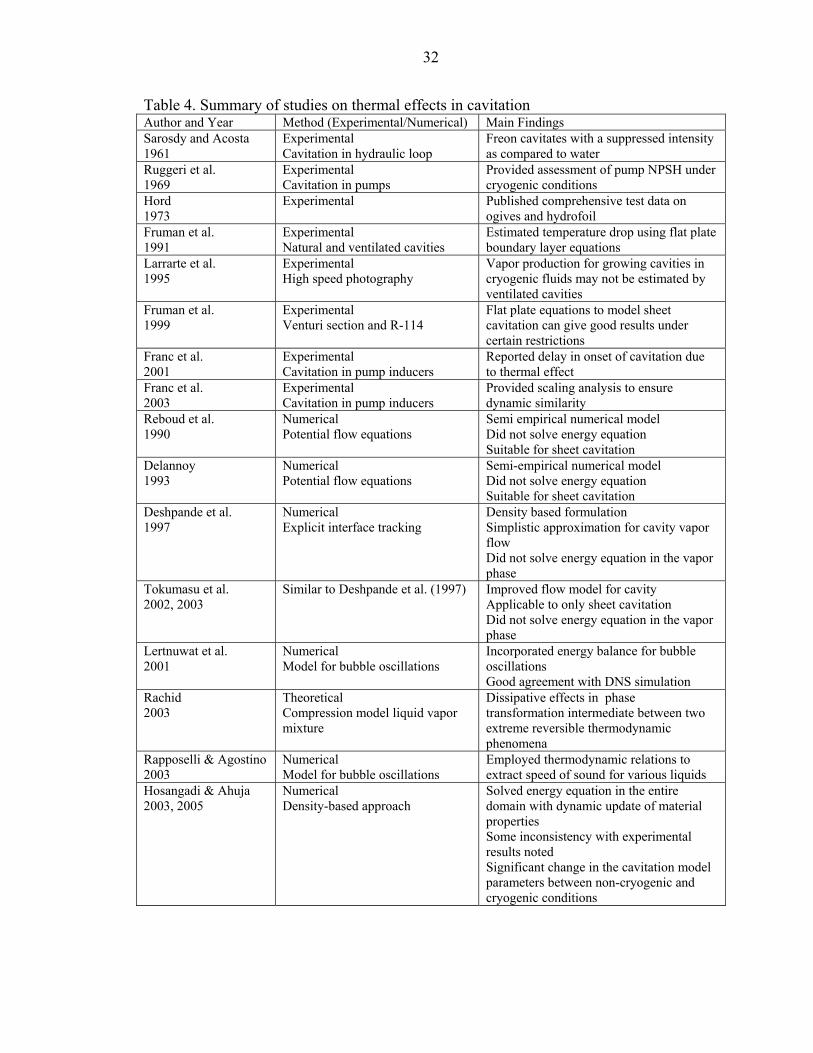
The above review (summarized in Table 4) points out the limited effort and the
wide scope for improving numerical modeling of thermal effects in cryogenic cavitation.
A broadly applicable and more robust numerical methodology is expected to be a
significant asset to prediction and critical investigation of cryogenic cavitation.
32
Table 4. Summary of studies on thermal effects in cavitation Author and Year Method (Experimental/Numerical) Main Findings Sarosdy and Acosta 1961
Experimental Cavitation in hydraulic loop
Freon cavitates with a suppressed intensity as compared to water
Ruggeri et al. 1969
Experimental Cavitation in pumps
Provided assessment of pump NPSH under cryogenic conditions
Hord 1973
Experimental Published comprehensive test data on ogives and hydrofoil
Fruman et al. 1991
Experimental Natural and ventilated cavities
Estimated temperature drop using flat plate boundary layer equations
Larrarte et al. 1995
Experimental High speed photography
Vapor production for growing cavities in cryogenic fluids may not be estimated by ventilated cavities
Fruman et al. 1999
Experimental Venturi section and R-114
Flat plate equations to model sheet cavitation can give good results under certain restrictions
Franc et al. 2001
Experimental Cavitation in pump inducers
Reported delay in onset of cavitation due to thermal effect
Franc et al. 2003
Experimental Cavitation in pump inducers
Provided scaling analysis to ensure dynamic similarity
Reboud et al. 1990
Numerical Potential flow equations
Semi empirical numerical model Did not solve energy equation Suitable for sheet cavitation
Delannoy 1993
Numerical Potential flow equations
Semi-empirical numerical model Did not solve energy equation Suitable for sheet cavitation
Deshpande et al. 1997
Numerical Explicit interface tracking
Density based formulation Simplistic approximation for cavity vapor flow Did not solve energy equation in the vapor phase
Tokumasu et al. 2002, 2003
Similar to Deshpande et al. (1997) Improved flow model for cavity Applicable to only sheet cavitation Did not solve energy equation in the vapor phase
Lertnuwat et al. 2001
Numerical Model for bubble oscillations
Incorporated energy balance for bubble oscillations Good agreement with DNS simulation
Rachid 2003
Theoretical Compression model liquid vapor mixture
Dissipative effects in phase transformation intermediate between two extreme reversible thermodynamic phenomena
Rapposelli & Agostino 2003
Numerical Model for bubble oscillations
Employed thermodynamic relations to extract speed of sound for various liquids
Hosangadi & Ahuja 2003, 2005
Numerical Density-based approach
Solved energy equation in the entire domain with dynamic update of material properties Some inconsistency with experimental results noted Significant change in the cavitation model parameters between non-cryogenic and cryogenic conditions

33
CHAPTER 3 STEADY STATE COMPUTATIONS
This chapter firstly delineates the governing equations that are employed in
obtaining steady-state solutions to various cases on cryogenic cavitation. Theoretical
formulation/derivation and computational implementation of various models, namely
cavitation, turbulence, compressibility, and thermal modeling aspects, are further
highlighted. The boundary conditions and steady-state results yielded by the
computational procedure are discussed in detail following the description of the basic
framework.
3.1 Governing Equations
The set of governing equations for cryogenic cavitation under the single-fluid
modeling strategy comprises the conservative form of the Favre-averaged Navier-Stokes
equations, the enthalpy equation, the k ε− two-equation turbulence closure, and a
transport equation for the liquid volume fraction. The mass-continuity, momentum,
enthalpy, and cavitation model equations are given below:
( )0m jm
j
ut x
ρρ ∂∂+ =
∂ ∂ (3.1)
( )( ) 2[( )( )]3
m i j jm i i kt ij
j i j j i k
u u uu u upt x x x x x x
ρρ µ µ δ∂ ∂∂ ∂ ∂∂ ∂
+ = − + + + −∂ ∂ ∂ ∂ ∂ ∂ ∂
(3.2)
[ ( )] [ ( )] [( ) ]Pr Pr
tm v m j v
j j L t j
hh f L u h f Lt x x x
µµρ ρ∂ ∂ ∂ ∂+ + + = +
∂ ∂ ∂ ∂ (3.3)
34
( )l jl
j
um m
t xαα + −∂∂
+ = +∂ ∂
& & (3.4)
We neglect the effects of compressible work and viscous dissipation from the energy
equation because the temperature field in cryogenic cavitation is mainly dictated by the
phenomenon of evaporative cooling. Here, the mixture density, sensible enthalpy, and the
vapor mass fraction are respectively expressed as:
(1 )m l l v lρ ρ α ρ α= + − (3.5)
Ph C T= (3.6)
(1 )v lv
m
f ρ αρ−
= (3.7)
The general framework of the Navier-Stokes solver (Senocak and Shyy 2002,
Thakur et al. 2002) employs a pressure-based algorithm and the finite-volume approach.
The governing equations are solved on multi-block, structured, curvilinear grids. The
viscous terms are discretized by second-order accurate central differencing while the
convective terms are approximated by the second-order accurate Controlled Variations
Scheme (CVS) (Shyy and Thakur 1994). The use of CVS scheme prevents oscillations
under shock-like expansion caused by the evaporation source term in the cavitation
model, while retaining second order of formal accuracy.
Steady-state computations are performed by discounting the time-derivative terms
in the governing equations and relaxing each equation to ensure a stable convergence to a
steady state. The pressure-velocity coupling is implemented through the SIMPLEC
(Versteeg and Malalasekera 1995) type of algorithm, cast in a combined Cartesian-
contravariant formulation (Thakur et al. 2002) for the dependent and flux variables,
respectively, followed by adequate relaxation for each governing equation, to obtain
35
steady-state results. The physical properties are updated, as explained earlier, after every
iteration.
3.1.1. Cavitation Modeling
Physically, the cavitation process is governed by thermodynamics and kinetics of
the phase change process. The liquid-vapor conversion associated with the cavitation
process is modeled through m+& and m−& terms in Eq. (3.4), which respectively represent,
condensation and evaporation. The particular form of these phase transformation rates,
which in case of cryogenic fluids also dictates the heat transfer process, forms the basis of
the cavitation model. Given below are the three modeling approaches probed in the
present study.
3.1.1.1 Merkle et al. Model
The liquid-vapor condensation rates for this particular model are given as (Merkle
et al. 1998):
2
2
Min(0, )(0.5 )
Max(0, )(1 )(0.5 )
dest l v l
v l
prod v l
l
C p pmU t
C p pm
U t
ρ αρ ρ
αρ
−
∞ ∞
+
∞ ∞
−=
− −=
&
&
(3.8)
Here, 1.0destC = and 80.0prodC = are empirical constants tuned by validating the
numerical results with experimental data. The time scale ( t∞ ) in the equation is defined as
the ratio of the characteristic length scale to the reference velocity scale ( /t D U∞ ∞= ).
3.1.1.2 Sharp Interfacial Dynamics Model (IDM)
The source terms of this model are derived by applying mass and momentum
balance across the cavity interface and appropriately eliminating the unquantifiable terms
(Senocak and Shyy 2002, 2004a, 2004b).
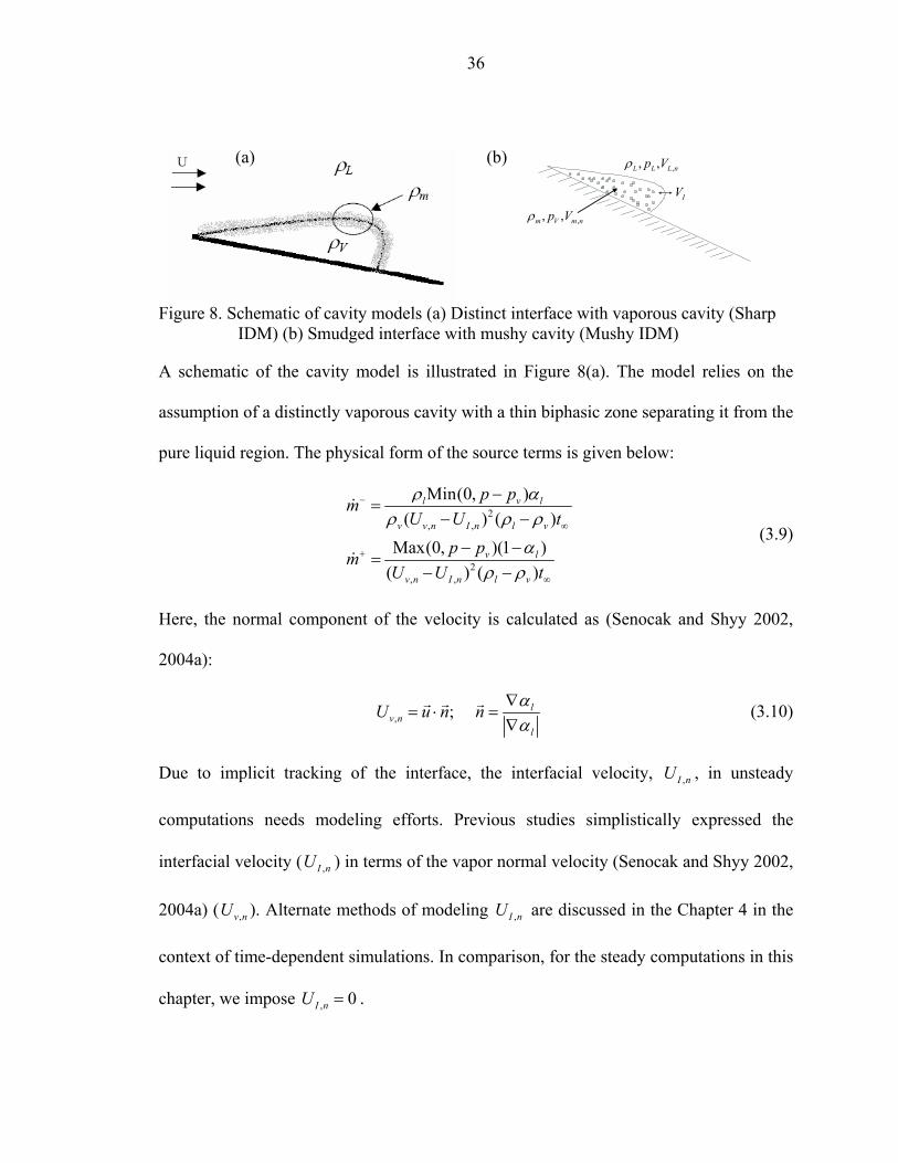
36
Figure 8. Schematic of cavity models (a) Distinct interface with vaporous cavity (Sharp
IDM) (b) Smudged interface with mushy cavity (Mushy IDM)
A schematic of the cavity model is illustrated in Figure 8(a). The model relies on the
assumption of a distinctly vaporous cavity with a thin biphasic zone separating it from the
pure liquid region. The physical form of the source terms is given below:
2, ,
2, ,
Min(0, )( ) ( )
Max(0, )(1 )( ) ( )
l v l
v v n I n l v
v l
v n I n l v
p pmU U t
p pmU U t
ρ αρ ρ ρ
αρ ρ
−
∞
+
∞
−=
− −
− −=
− −
&
&
(3.9)
Here, the normal component of the velocity is calculated as (Senocak and Shyy 2002,
2004a):
, ; lv n
l
U u n n αα
∇= ⋅ =
∇r r r (3.10)
Due to implicit tracking of the interface, the interfacial velocity, ,I nU , in unsteady
computations needs modeling efforts. Previous studies simplistically expressed the
interfacial velocity ( ,I nU ) in terms of the vapor normal velocity (Senocak and Shyy 2002,
2004a) ( ,v nU ). Alternate methods of modeling ,I nU are discussed in the Chapter 4 in the
context of time-dependent simulations. In comparison, for the steady computations in this
chapter, we impose , 0I nU = .
,, ,m V m np Vρ
,, ,L L L np Vρ
IV
(a) (b)
37
3.1.1.3 Mushy Interfacial Dynamics Model (IDM)
Experimental visualizations of cryogenic cavitation (Sarosdy and Acosta 1961;
Hord 1973a, 1973b) have clearly indicated a mushy nature of the cavity. This salient
characteristic of cryogenic cavitation solicits an adaptation of the existing cavitation
model to reflect the same. We choose the Sharp IDM (Senocak and Shyy 2004a) in our
analysis because of its stronger physical reasoning. The following discussion serves to
revise the above cavitation model by re-examining its derivation and assumptions, to
appropriately accommodate the features of cryogenic cavitation. Although we refer the
reader to literature (Senocak and Shyy 2004a) for the detailed derivation of the earlier
model, we underscore the differences between the two approaches in the proceeding
description.
Figure 8(b) – representing Mushy IDM - depicts a cavity where the vapor pressure
is a function of the local temperature, and the nature of cavitation demonstrates a weak
intensity and consequently less probability for existence of pure vapor phase inside the
cavitation zone. In comparison, Figure 8(a) – representing Sharp IDM - depicts a cavity
typically produced under regular conditions (no temperature effects), characterized by a
thin biphasic region separating the two phases. We initiate our approach similar to
Senocak and Shyy (2004a) by formulating the mass and momentum balance condition at
the cavity interface, which is assumed to separate the liquid and mixture regions. We
neglect the viscous terms and surface tension effects from equation (3.12) assuming high
Re flows and large cavity sizes respectively.
, , , ,( ) ( )l l n I n m m n I nU U U Uρ ρ− = − (3.11)
2 2, , , ,( ) ( )l v m m n I n l l n I np p U V U Vρ ρ− = − − − (3.12)
38
It is noteworthy that Senocak and Shyy (2004a) formulated the above equations midst the
pure vapor and mixture regions while hypothesizing an interface between the two. The
two models differ in terms of their interpretation of the cavity attributes, namely, the
density and the velocity field within the cavitation zone, while adhering to the
fundamental idea of mass/momentum balance. Since we attribute a “frothy” nature to the
cavity, the term .u nr r is largely expected to represent the mixture normal velocity.
Accounting for this fact, we eliminate the ,l nU term from equation (3.12) using equation
(3.11) as shown below.
22 2
, , , ,( ) ( )ml v m m n I n m n I n
l
p p U U U Uρρρ
− = − − − (3.13)
Further re-arrangement progressively yields the following equations:
2 2, , , ,( ) [1 ] ( )m l v
l v m m n I n m m n I n vl l
p p U U U Uρ ρ ρρ ρ αρ ρ
−− = − − = − (3.14)
2 2, , , ,
( ) ( ) ( )( )( ) ( )( )
l l v l l vv v l
m l v m n I n m l v m n I n
p p p pU U U U
ρ ρα α αρ ρ ρ ρ ρ ρ
− −= = +
− − − − (3.15)
2 2, , , ,
( ) ( )(1 )( )( ) ( )( )
l l v l l l v lv
m l v m n I n m l v m n I n
p p p pU U U U
ρ α ρ ααρ ρ ρ ρ ρ ρ
− − −= +
− − − − (3.16)
From standpoint of formulating source terms for the lα transport equation, we firstly
normalize the above equation by the overall convective timescale ( /t D U∞ ∞= ).
Secondly, we apply conditional statements on the pressure terms to invoke either
evaporation or condensation depending on the local pressure and vapor pressure (refer to
Senocak and Shyy 2002 & 2004a). Lastly, we assume that the volume rates for the
individual phases are interchangeable barring the sign convention. For instance, the

39
evaporation term, m−& , in the equationlα − or equationvα − would bear the same
magnitude, but negative or positive sign, respectively. We thus obtain the following
source terms from the above analysis:
2, ,
2, ,
Min(0, )( ) ( )Max(0, )(1 )
( ) ( )
l v l
m m n I n l v
l v l
m m n I n l v
p pmU U t
p pmU U t
ρ αρ ρ ρ
ρ αρ ρ ρ
−
∞
+
∞
−=
− −
− −=
− −
&
&
(3.17)
The normal component of the mixture velocity is expressed as shown in equation (3.10)
and consistent with the normal component of the vapor velocity employed by the Sharp
IDM.
A comparison with equation (3.9) shows that a factor of /v mρ ρ weakens the
evaporation term while a factor of /l mρ ρ strengthens the condensation term of the Sharp
IDM to yield the Mushy IDM. For instance, at a nominal density ratio of 100 and
0.5lα = , the value of /v mρ ρ and /l mρ ρ is 21.82 10−× and 1.82, respectively. In terms of
order of magnitude, the difference between the evaporation terms of the two models is
relatively more pronounced than the condensation terms, especially for high liquid-vapor
density ratios. Given this fact, we attempt to make the Mushy IDM consistent with the
Sharp IDM by providing an exponential transition of the evaporation source term from
one model to the other as a function of the phase fraction ( lα ). Specifically, we employ
the evaporation term from equation (3.17) as we get closer to the liquid region, and that
from equation (3.9) as we get farther from the liquid region. In comparison, the
condensation term from equation (3.17), which is mainly expected to be active in the
region outlining the ‘vaporous’ portion of the cavity, is unaltered. In summary, the
Mushy IDM is eventually formulated as shown below.
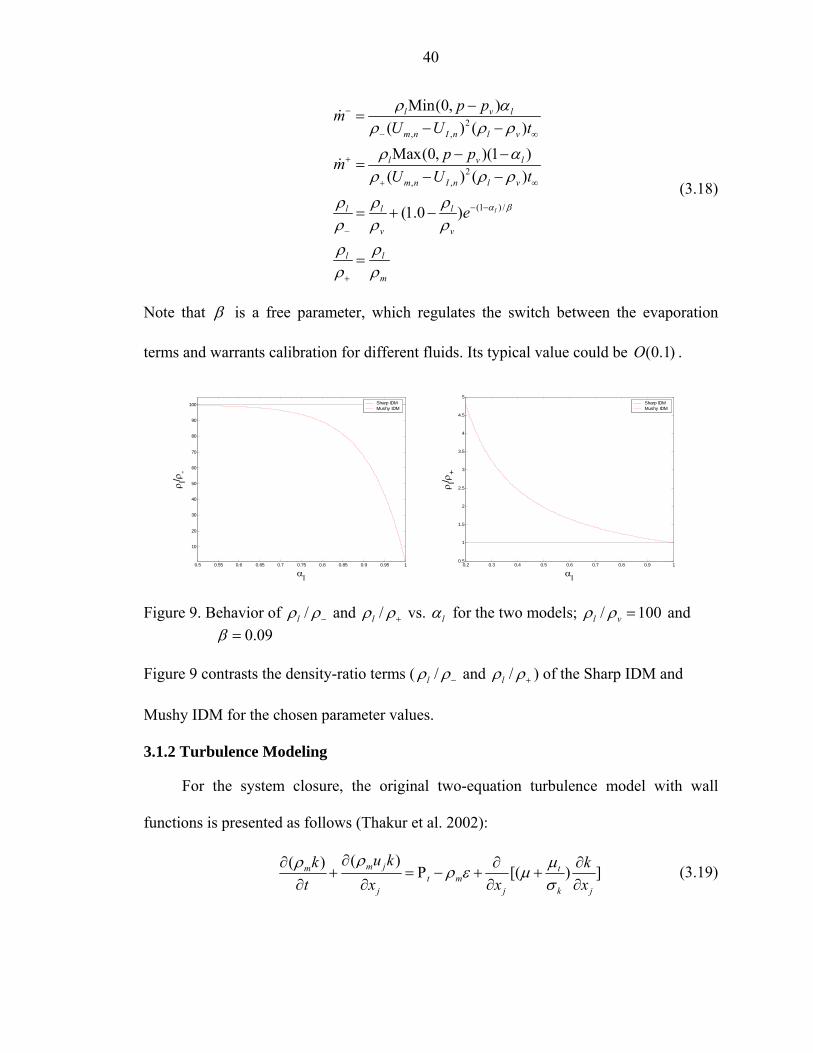
40
2, ,
2, ,
(1 ) /
Min(0, )( ) ( )Max(0, )(1 )
( ) ( )
(1.0 ) l
l v l
m n I n l v
l v l
m n I n l v
l l l
v v
l l
m
p pmU U t
p pmU U t
e α β
ρ αρ ρ ρ
ρ αρ ρ ρ
ρ ρ ρρ ρ ρρ ρρ ρ
−
− ∞
+
+ ∞
− −
−
+
−=
− −
− −=
− −
= + −
=
&
&
(3.18)
Note that β is a free parameter, which regulates the switch between the evaporation
terms and warrants calibration for different fluids. Its typical value could be (0.1)O .
0.5 0.55 0.6 0.65 0.7 0.75 0.8 0.85 0.9 0.95 1
10
20
30
40
50
60
70
80
90
100
αl
ρ l/ ρ-
Sharp IDMMushy IDM
0.2 0.3 0.4 0.5 0.6 0.7 0.8 0.9 10.5
1
1.5
2
2.5
3
3.5
4
4.5
5
αl
ρ l/ ρ+
Sharp IDMMushy IDM
Figure 9. Behavior of /lρ ρ− and /lρ ρ+ vs. lα for the two models; / 100l vρ ρ = and 0.09β =
Figure 9 contrasts the density-ratio terms ( /lρ ρ− and /lρ ρ+ ) of the Sharp IDM and
Mushy IDM for the chosen parameter values.
3.1.2 Turbulence Modeling
For the system closure, the original two-equation turbulence model with wall
functions is presented as follows (Thakur et al. 2002):
( )( ) [( ) ]m jm tt m
j j k j
u kk kt x x x
ρρ µρ ε µσ
∂∂ ∂ ∂+ = Ρ − + +
∂ ∂ ∂ ∂ (3.19)
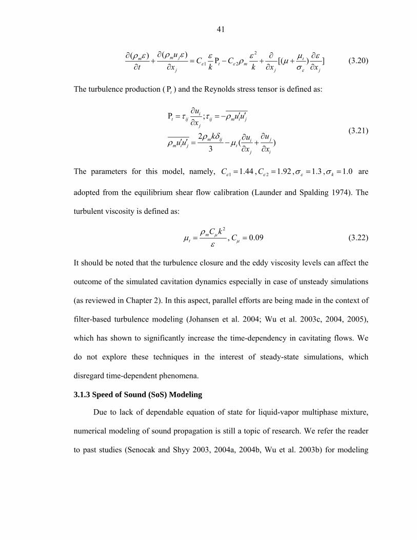
41
2
1 2
( )( ) P [( ) ]m jm tt m
j j j
uC C
t x k k x xε εε
ρ ερ ε µε ε ερ µσ
∂∂ ∂ ∂+ = − + +
∂ ∂ ∂ ∂ (3.20)
The turbulence production ( Pt ) and the Reynolds stress tensor is defined as:
P ;
2( )
3
it ij ij m i j
j
m ij jim i j t
j i
u u ux
k uuu ux x
τ τ ρ
ρ δρ µ
∂ ′ ′= = −∂
∂∂′ ′ = − +∂ ∂
(3.21)
The parameters for this model, namely, 1 1.44Cε = , 2 1.92Cε = , 1.3εσ = , 1.0kσ = are
adopted from the equilibrium shear flow calibration (Launder and Spalding 1974). The
turbulent viscosity is defined as:
2
, 0.09mt
C kCµ
µ
ρµ
ε= = (3.22)
It should be noted that the turbulence closure and the eddy viscosity levels can affect the
outcome of the simulated cavitation dynamics especially in case of unsteady simulations
(as reviewed in Chapter 2). In this aspect, parallel efforts are being made in the context of
filter-based turbulence modeling (Johansen et al. 2004; Wu et al. 2003c, 2004, 2005),
which has shown to significantly increase the time-dependency in cavitating flows. We
do not explore these techniques in the interest of steady-state simulations, which
disregard time-dependent phenomena.
3.1.3 Speed of Sound (SoS) Modeling
Due to lack of dependable equation of state for liquid-vapor multiphase mixture,
numerical modeling of sound propagation is still a topic of research. We refer the reader
to past studies (Senocak and Shyy 2003, 2004a, 2004b, Wu et al. 2003b) for modeling

42
options, their impact and issues, and just outline the currently employed SoS model
below.
SoS (1 )lC Cρ α= = − (3.23)
The density correction term in the continuity equation is thus coupled to the pressure
correction term as shown below.
' 'm C pρρ = (3.24)
Senocak and Shyy (2002 & 2004a) suggested an O(1) value for the constant C to
expedite the convergence of the iterative computational algorithm. However, their
recommendation is valid under normalized values for inlet velocity and liquid density.
Since we employ dimensional form of equations for cryogenic fluids, we suggest an
O( 21/U∞ ) value for C, which is consistent with the above suggestion in terms of the Mach
number regime. The speed of sound affects the numerical calculation via the pressure
correction equation by conditionally endowing it with a convective-diffusive form in the
mixture region. In the pure liquid region, we recover the diffusive form of the pressure
equation.
3.1.4 Thermal Modeling
The thermal effects are mainly regulated by the evaporative cooling process, which
is further manifested by the temperature dependence of physical properties and vapor
pressure.
3.1.4.1 Fluid property update
In the present study, we subject all the physical properties, namely,
, , , , , , and l v v Pp C K Lρ ρ µ to temperature dependence.
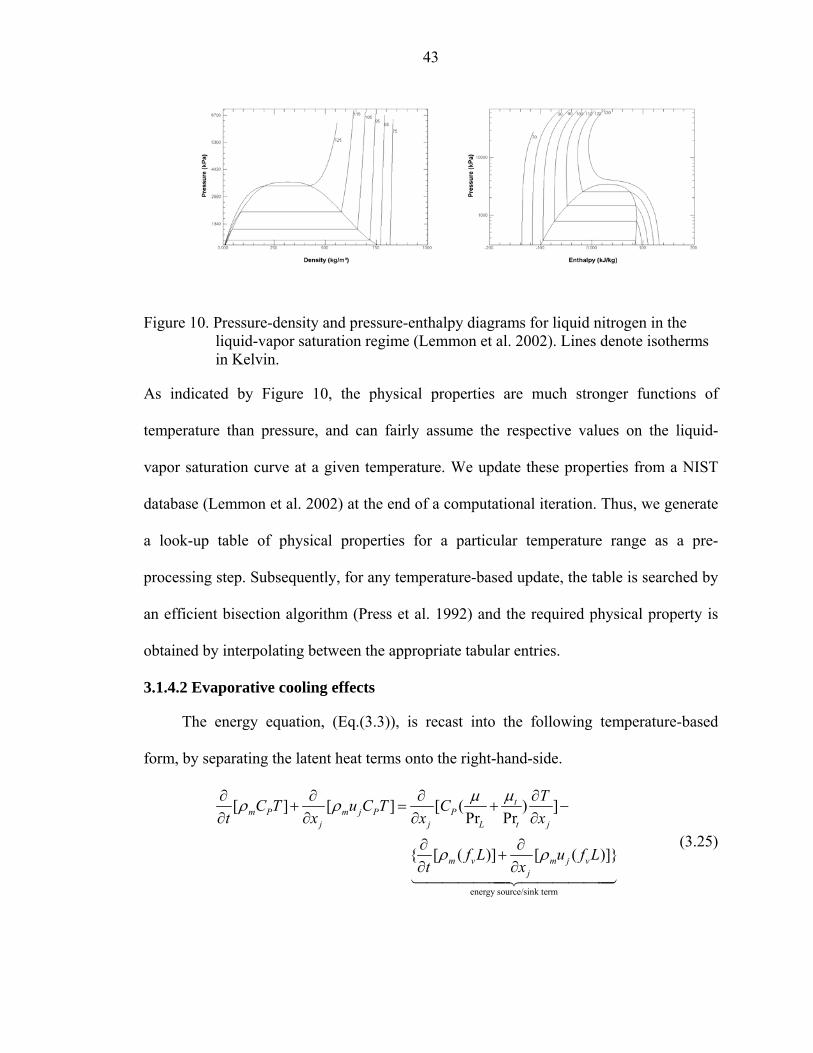
43
Figure 10. Pressure-density and pressure-enthalpy diagrams for liquid nitrogen in the liquid-vapor saturation regime (Lemmon et al. 2002). Lines denote isotherms in Kelvin.
As indicated by Figure 10, the physical properties are much stronger functions of
temperature than pressure, and can fairly assume the respective values on the liquid-
vapor saturation curve at a given temperature. We update these properties from a NIST
database (Lemmon et al. 2002) at the end of a computational iteration. Thus, we generate
a look-up table of physical properties for a particular temperature range as a pre-
processing step. Subsequently, for any temperature-based update, the table is searched by
an efficient bisection algorithm (Press et al. 1992) and the required physical property is
obtained by interpolating between the appropriate tabular entries.
3.1.4.2 Evaporative cooling effects
The energy equation, (Eq.(3.3)), is recast into the following temperature-based
form, by separating the latent heat terms onto the right-hand-side.
energy source/sink term
[ ] [ ] [ ( ) ]Pr Pr
[ ( )] [ ( )]
tm P m j P P
j j L t j
m v m j vj
TC T u C T Ct x x x
f L u f Lt x
µµρ ρ
ρ ρ
∂ ∂ ∂ ∂+ = + −
∂ ∂ ∂ ∂
∂ ∂+
∂ ∂144444424444443
(3.25)
44
As seen from equation (3.25), the ‘lumped’ latent heat terms manifest as a non-linear
source term into the energy equation and physically represent the latent heat transfer rate.
The spatial variation of thermodynamic properties and the evaporative cooling effect are
intrinsically embedded into this transport-based source term. We calculate the source
term by discretizing the associated derivatives in concert with the numerical schemes
applied to the terms on the left-hand-side of the equation.
3.1.5 Boundary Conditions
The boundary conditions are implemented by stipulating the values of the velocity
components (obtained from the experimental data), phase fraction, temperature, and
turbulence quantities at the inlet. Furthermore, at the walls, pressure, phase fraction, and
turbulence quantities are extrapolated, along with applying the no-slip and adiabatic
condition on the velocity and temperature, respectively. Pressure and other variables are
extrapolated at the outlet boundaries, while enforcing global mass conservation by
rectifying of the outlet velocity components. In addition, we also hold the pressure at the
reference pressure point constantly at the reference value (specified by the experiments).
This is simply done by adjusting the linear coefficients of the pressure correction
equation at that point, to yield zero correction, at every iteration. Symbolically, this is
achieved by substituting 1, 0p p pP nb PA A B= = = into the following linear equation at the
point of interest:
' 'p pP P nb nb PA p A p B= +∑ (3.26)
We observe that this adjustment imparts robustness and stability to the computation.
45
3.2 Results and Discussion
In this section, we firstly observe the nuances of the Mushy IDM on non-cryogenic
cases. The purpose is to distill the impact solely caused due to the source term change
between the Sharp and Mushy IDM, and contrast it against commonly referred
experimental and computational results. Later, we extend our computations to the
variable temperature environment of cryogenic fluids. Specifically, we observe the effect
of the temperature field on the nature of cavitation under similar conditions. Furthermore,
we assess the Mushy IDM with available experimental data (pressure and temperature)
and compare it with the alternative cavitation models. In the process of calibrating the
cavitation models for cryogenic fluids, we perform a global sensitivity analysis to
evaluate the sensitivity of the prediction to changes in material properties and model
parameters. We offer discussion about optimizing the model performance based on our
sensitivity study.
3.2.1 Cavitation in Non-cryogenic Fluids
As mentioned above, we register first the impact of the Mushy IDM on non-
cryogenic cases. In this initial exercise, we consider the influence of the mushy
formulation only to the liquid boundary layer encompassing the cavity. Symbolically, we
implement the following formulation for the non-cryogenic cases.
2, ,
2, ,
Min(0, )( ) ( )Max(0, )(1 )
( ) ( )
if 0.99 else
if 0.99 1 else
l v l
m n I n l v
l v l
m n I n l v
l l l ll
v m
l l ll
m
p pmU U t
p pmU U t
ρ αρ ρ ρ
ρ αρ ρ ρ
ρ ρ ρ ραρ ρ ρ ρρ ρ ραρ ρ ρ
−
− ∞
+
+ ∞
− −
+ +
−=
− −
− −=
− −
≤ = =
≤ = =
&
&
(3.27)
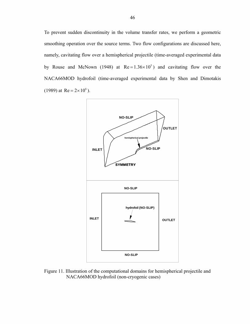
46
To prevent sudden discontinuity in the volume transfer rates, we perform a geometric
smoothing operation over the source terms. Two flow configurations are discussed here,
namely, cavitating flow over a hemispherical projectile (time-averaged experimental data
by Rouse and McNown (1948) at 5Re 1.36 10= × ) and cavitating flow over the
NACA66MOD hydrofoil (time-averaged experimental data by Shen and Dimotakis
(1989) at 6Re 2 10= × ).
NO-SLIP
OUTLET
INLET
SYMMETRYSYMMETRY
NO-SLIP
hemispherical projectile
INLET OUTLET
NO-SLIP
NO-SLIP
hydrofoil (NO-SLIP)
Figure 11. Illustration of the computational domains for hemispherical projectile and NACA66MOD hydrofoil (non-cryogenic cases)

47
The computational domains for the two geometries are depicted in Figure 11. We
consider two grids with 158 66× and 292 121× points for the hemispherical geometry,
which is axisymmetric. In case of the NACA66MOD hydrofoil, we defer to the judgment
of a previous study (Senocak and Shyy 2004a), and employ the finer grid from that study.
s/D
Cp
0 1 2 3 4
-0.5
0
0.5
1
Mushy IDM - 158 x 66 gridMushy IDM - 292 x 121 gridExp. data
s/D
Cp
0 1 2 3 4
-0.5
0
0.5
1
Sharp IDMMerkle et al. ModelMushy IDMExp. data
Figure 12. Pressure coefficients over the hemispherical body ( 0.4σ = ); D is the diameter of the hemispherical projectile. (a) Impact of grid refinement for Mushy IDM (b) Comparison between pressure coefficients of different models on the coarse grid
We investigate the sensitivity of Mushy IDM to grid refinement for the two
hemispherical body grids through the surface pressure plots in Figure 12. Note that the
refinement factor in the vicinity of cavitating region is roughly 2.5-3. Figure 12(a)
indicates a noticeable, though modest, effect of the grid refinement on the surface
pressure. This can be mainly attributed to the grid-dependent geometric smoothing
operation, which smears the mushy formulation over a larger portion in the coarser grid.
Nonetheless, both the grids produce solutions that match the experimental data
reasonably well. Furthermore, it is important to mention that the near-wall nodes of the
coarser grid lie in the log-layer of the turbulent boundary layer enabling appropriate use
of the wall function (Versteeg and Malalasekera 1995), while the fine grid is over-refined
(a) (b)
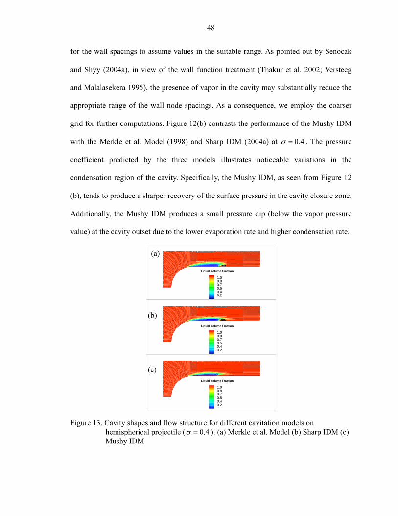
48
for the wall spacings to assume values in the suitable range. As pointed out by Senocak
and Shyy (2004a), in view of the wall function treatment (Thakur et al. 2002; Versteeg
and Malalasekera 1995), the presence of vapor in the cavity may substantially reduce the
appropriate range of the wall node spacings. As a consequence, we employ the coarser
grid for further computations. Figure 12(b) contrasts the performance of the Mushy IDM
with the Merkle et al. Model (1998) and Sharp IDM (2004a) at 0.4σ = . The pressure
coefficient predicted by the three models illustrates noticeable variations in the
condensation region of the cavity. Specifically, the Mushy IDM, as seen from Figure 12
(b), tends to produce a sharper recovery of the surface pressure in the cavity closure zone.
Additionally, the Mushy IDM produces a small pressure dip (below the vapor pressure
value) at the cavity outset due to the lower evaporation rate and higher condensation rate.
1.00.80.70.50.40.2
Liquid Volume Fraction
1.00.80.70.50.40.2
Liquid Volume Fraction
1.00.80.70.50.40.2
Liquid Volume Fraction
Figure 13. Cavity shapes and flow structure for different cavitation models on hemispherical projectile ( 0.4σ = ). (a) Merkle et al. Model (b) Sharp IDM (c) Mushy IDM
(a)
(b)
(c)
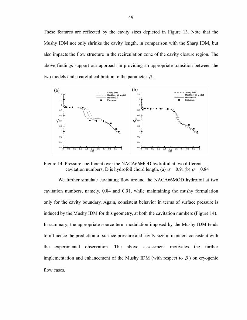
49
These features are reflected by the cavity sizes depicted in Figure 13. Note that the
Mushy IDM not only shrinks the cavity length, in comparison with the Sharp IDM, but
also impacts the flow structure in the recirculation zone of the cavity closure region. The
above findings support our approach in providing an appropriate transition between the
two models and a careful calibration to the parameter β .
x/D
-Cp
0 0.1 0.2 0.3 0.4 0.5 0.6 0.7 0.8 0.9 1-0.6
-0.4
-0.2
0
0.2
0.4
0.6
0.8
1
1.2
1.4Sharp IDMMerkle et al. ModelMushy IDMExp. data
x/D
-Cp
0 0.1 0.2 0.3 0.4 0.5 0.6 0.7 0.8 0.9 1-0.6
-0.4
-0.2
0
0.2
0.4
0.6
0.8
1
1.2
1.4Sharp IDMMerkle et al. ModelMushy IDMExp. data
Figure 14. Pressure coefficient over the NACA66MOD hydrofoil at two different cavitation numbers; D is hydrofoil chord length. (a) 0.91σ = (b) 0.84σ =
We further simulate cavitating flow around the NACA66MOD hydrofoil at two
cavitation numbers, namely, 0.84 and 0.91, while maintaining the mushy formulation
only for the cavity boundary. Again, consistent behavior in terms of surface pressure is
induced by the Mushy IDM for this geometry, at both the cavitation numbers (Figure 14).
In summary, the appropriate source term modulation imposed by the Mushy IDM tends
to influence the prediction of surface pressure and cavity size in manners consistent with
the experimental observation. The above assessment motivates the further
implementation and enhancement of the Mushy IDM (with respect to β ) on cryogenic
flow cases.
(a) (b)
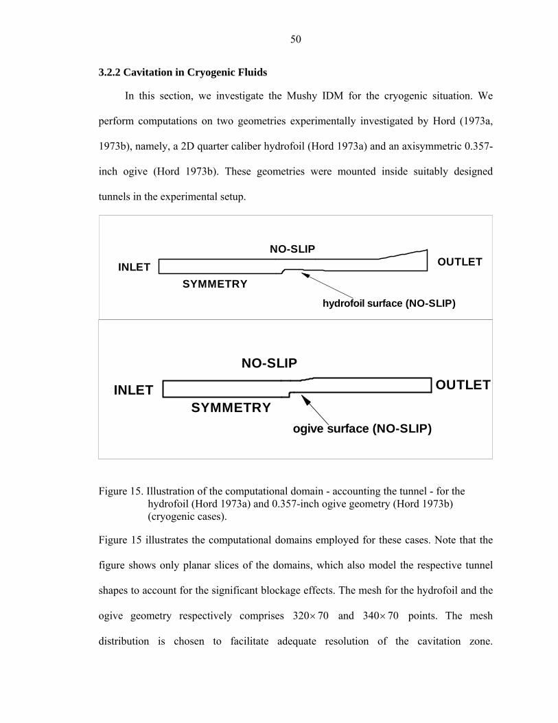
50
3.2.2 Cavitation in Cryogenic Fluids
In this section, we investigate the Mushy IDM for the cryogenic situation. We
perform computations on two geometries experimentally investigated by Hord (1973a,
1973b), namely, a 2D quarter caliber hydrofoil (Hord 1973a) and an axisymmetric 0.357-
inch ogive (Hord 1973b). These geometries were mounted inside suitably designed
tunnels in the experimental setup.
INLET OUTLETNO-SLIP
SYMMETRY
hydrofoil surface (NO-SLIP)
INLET OUTLETSYMMETRY
NO-SLIP
ogive surface (NO-SLIP)
Figure 15. Illustration of the computational domain - accounting the tunnel - for the hydrofoil (Hord 1973a) and 0.357-inch ogive geometry (Hord 1973b) (cryogenic cases).
Figure 15 illustrates the computational domains employed for these cases. Note that the
figure shows only planar slices of the domains, which also model the respective tunnel
shapes to account for the significant blockage effects. The mesh for the hydrofoil and the
ogive geometry respectively comprises 320 70× and 340 70× points. The mesh
distribution is chosen to facilitate adequate resolution of the cavitation zone.
51
Furthermore, the near-wall resolution over all the no-slip planes (cavitating geometries
and tunnel walls) accounts for deployment of wall functions (Thakur et al. 2002;
Versteeg and Malalasekera 1995).
Table 5. Flow cases chosen for the hydrofoil geometry. Fluid: Case name: Inlet temperature: Freestream Re: Cav. No. (σ∞ ):
Liq. N2 283B 77.65 K 64.7 10× 1.73
Liq. N2 290C 83.06 K 69.1 10× 1.70
Liq. N2 296B 88.54 K 71.1 10× 1.61
Liq. H2 248C 20.46 K 71.8 10× 1.60
Liq. H2 249D 20.70 K 72.0 10× 1.57
Liq. H2 255C 22.20 K 72.5 10× 1.49
Source: Hord (1973a)
Table 6. Flow cases chosen for the ogive geometry. Fluid: Case name: Inlet temperature: Freestream Re: Cav. No. (σ∞ ):
Liq. N2 312D 83.00 K 69.0 10× 0.46
Liq. N2 322E 88.56 K 71.2 10× 0.44
Liq. H2 349B 21.33 K 72.3 10× 0.38
Source: Hord (1973b)
Statistically-averaged pressure and temperature data are available for the two geometries
at five probe locations over the body surfaces. The experimental findings report varying
amounts of unsteady behavior in the cavity closure regions, although no case-specific
information or data/visuals are available in that context. Hord conducted a series of
experiments over both the geometries, using liquid nitrogen and hydrogen, by varying the
inlet velocity, temperature, and pressure. In our computations, we have selected several

52
cases, referenced alphanumerically in the reports by Hord (1973a, 1973b), with different
freestream temperatures and cavitation numbers (see Table 5 and Table 6).
x/D
Cp
-1 0 1 2 3 4 5-3
-2.5
-2
-1.5
-1
-0.5
0
0.5
1Computed pressureHord, 1973 (incipient data)
x/D
Cp
0 2 4-2
-1.5
-1
-0.5
0
0.5
1
1.5Computed pressureHord, 1973 (incipient data)
Figure 16. Non-cavitating pressure distribution (a) case ‘290C’, D represents hydrofoil thickness and x represents distance from the circular bend (b) case ‘312D’, D represents ogive diameter and x represents distance from the leading edge
To validate the use of real fluid properties, we obtain the single-phase flow
solution to cases ‘290C’ (hydrofoil; Re= 69.1 10× , 1.7σ∞ = ) and ‘312D’ (ogive;
Re= 69.0 10× , 0.46σ∞ = ), and compare the computed surface pressure with the
experimentally measured pressure under incipient (virtually non-cavitating) conditions.
Figure 16 demonstrates good agreement between the numerical and experimental data for
both the geometries, and corroborates the correct input of physical properties.
3.2.2.1 Sensitivity analyses
In general, cryogenic computations are prone to uncertainty due to a multitude of
inputs, in contrast to the non-cryogenic conditions. The cavitation model parameters,
namely, , , and dest prodC C t∞ , have been selected largely based on the non-cryogenic
conditions. Furthermore, the solutions can exhibit substantial sensitivity with respect to
minor changes in the flow environment. For example, the uncertainties involved in the
(a) (b)
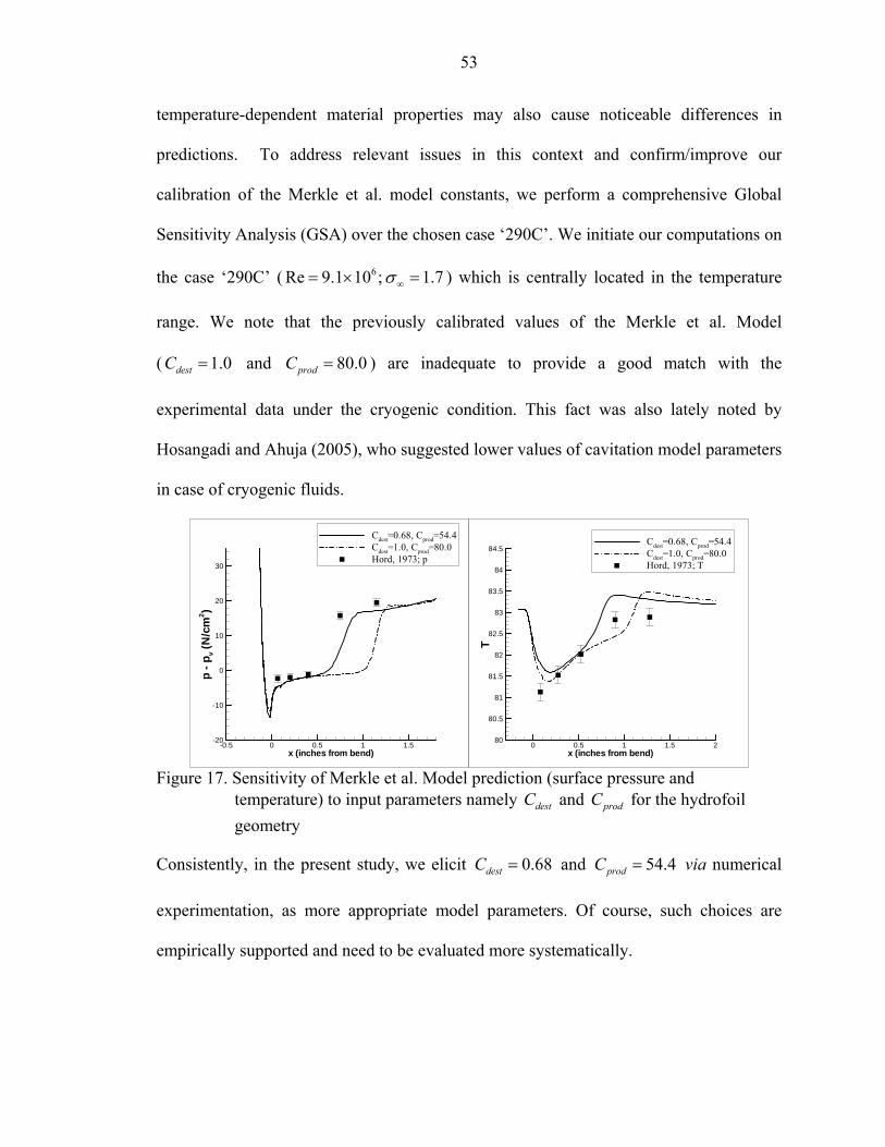
53
temperature-dependent material properties may also cause noticeable differences in
predictions. To address relevant issues in this context and confirm/improve our
calibration of the Merkle et al. model constants, we perform a comprehensive Global
Sensitivity Analysis (GSA) over the chosen case ‘290C’. We initiate our computations on
the case ‘290C’ ( 6Re 9.1 10 ; 1.7σ∞= × = ) which is centrally located in the temperature
range. We note that the previously calibrated values of the Merkle et al. Model
( 1.0=destC and 80.0=prodC ) are inadequate to provide a good match with the
experimental data under the cryogenic condition. This fact was also lately noted by
Hosangadi and Ahuja (2005), who suggested lower values of cavitation model parameters
in case of cryogenic fluids.
x (inches from bend)
p-p
v(N
/cm
2 )
-0.5 0 0.5 1 1.5-20
-10
0
10
20
30
Cdest=0.68, Cprod=54.4Cdest=1.0, Cprod=80.0Hord, 1973; p
x (inches from bend)
T
0 0.5 1 1.5 280
80.5
81
81.5
82
82.5
83
83.5
84
84.5Cdest=0.68, Cprod=54.4Cdest=1.0, Cprod=80.0Hord, 1973; T
Figure 17. Sensitivity of Merkle et al. Model prediction (surface pressure and
temperature) to input parameters namely destC and prodC for the hydrofoil geometry
Consistently, in the present study, we elicit 0.68destC = and 54.4prodC = via numerical
experimentation, as more appropriate model parameters. Of course, such choices are
empirically supported and need to be evaluated more systematically.
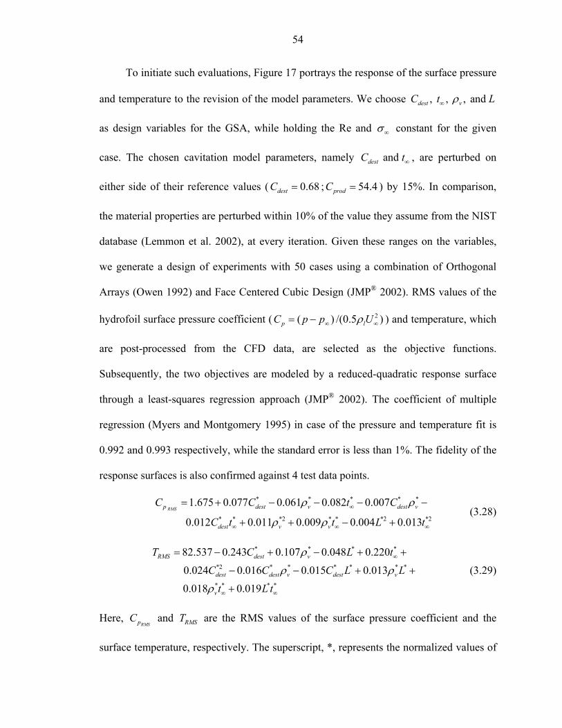
54
To initiate such evaluations, Figure 17 portrays the response of the surface pressure
and temperature to the revision of the model parameters. We choose , , , and dest vC t Lρ∞
as design variables for the GSA, while holding the Re and σ∞ constant for the given
case. The chosen cavitation model parameters, namely and destC t∞ , are perturbed on
either side of their reference values ( 0.68destC = ; 54.4prodC = ) by 15%. In comparison,
the material properties are perturbed within 10% of the value they assume from the NIST
database (Lemmon et al. 2002), at every iteration. Given these ranges on the variables,
we generate a design of experiments with 50 cases using a combination of Orthogonal
Arrays (Owen 1992) and Face Centered Cubic Design (JMP® 2002). RMS values of the
hydrofoil surface pressure coefficient ( 2( ) /(0.5 )p lC p p Uρ∞ ∞= − ) and temperature, which
are post-processed from the CFD data, are selected as the objective functions.
Subsequently, the two objectives are modeled by a reduced-quadratic response surface
through a least-squares regression approach (JMP® 2002). The coefficient of multiple
regression (Myers and Montgomery 1995) in case of the pressure and temperature fit is
0.992 and 0.993 respectively, while the standard error is less than 1%. The fidelity of the
response surfaces is also confirmed against 4 test data points.
* * * * *
* * *2 * * *2 *2
1.675 0.077 0.061 0.082 0.007
0.012 0.011 0.009 0.004 0.013RMSp dest v dest v
dest v v
C C t C
C t t L t
ρ ρ
ρ ρ∞
∞ ∞ ∞
= + − − − −
+ + − + (3.28)
* * * *
*2 * * * * * *
* * * *
82.537 0.243 0.107 0.048 0.220
0.024 0.016 0.015 0.013
0.018 0.019
RMS dest v
dest dest v dest v
v
T C L t
C C C L L
t L t
ρ
ρ ρ
ρ
∞
∞ ∞
= − + − + +
− − + +
+
(3.29)
Here, RMSpC and RMST are the RMS values of the surface pressure coefficient and the
surface temperature, respectively. The superscript, *, represents the normalized values of
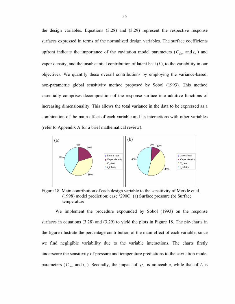
55
the design variables. Equations (3.28) and (3.29) represent the respective response
surfaces expressed in terms of the normalized design variables. The surface coefficients
upfront indicate the importance of the cavitation model parameters ( and destC t∞ ) and
vapor density, and the insubstantial contribution of latent heat (L), to the variability in our
objectives. We quantify these overall contributions by employing the variance-based,
non-parametric global sensitivity method proposed by Sobol (1993). This method
essentially comprises decomposition of the response surface into additive functions of
increasing dimensionality. This allows the total variance in the data to be expressed as a
combination of the main effect of each variable and its interactions with other variables
(refer to Appendix A for a brief mathematical review).
0%20%
38%
42%Latent heatVapor densityC_destt_infinity
1% 10%
43%
46%Latent heatVapor densityC_destt_infinity
Figure 18. Main contribution of each design variable to the sensitivity of Merkle et al.
(1998) model prediction; case ‘290C’ (a) Surface pressure (b) Surface temperature
We implement the procedure expounded by Sobol (1993) on the response
surfaces in equations (3.28) and (3.29) to yield the plots in Figure 18. The pie-charts in
the figure illustrate the percentage contribution of the main effect of each variable; since
we find negligible variability due to the variable interactions. The charts firstly
underscore the sensitivity of pressure and temperature predictions to the cavitation model
parameters ( and destC t∞ ). Secondly, the impact of vρ is noticeable, while that of L is
(a) (b)
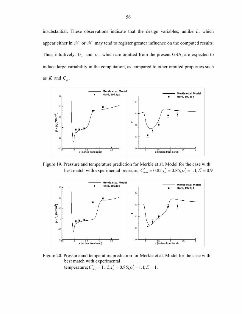
56
insubstantial. These observations indicate that the design variables, unlike L, which
appear either in m−& or m+& may tend to register greater influence on the computed results.
Thus, intuitively, U∞ and lρ , which are omitted from the present GSA, are expected to
induce large variability in the computation, as compared to other omitted properties such
as K and pC .
x (inches from bend)
p-p
v(N
/cm
2 )
-0.5 0 0.5 1 1.5-20
-10
0
10
20
30
Merkle et al. ModelHord, 1973; p
x (inches from bend)
T
0 0.5 1 1.5 280
81
82
83
84
Merkle et al. ModelHord, 1973; T
Figure 19. Pressure and temperature prediction for Merkle et al. Model for the case with best match with experimental pressure; * * * *0.85; 0.85; 1.1; 0.9dest vC t Lρ∞= = = =
x (inches from bend)
p-p
v(N
/cm
2 )
-0.5 0 0.5 1 1.5-20
-10
0
10
20
30
Merkle et al. ModelHord, 1973; p
x (inches from bend)
T
0 0.5 1 1.5 280
81
82
83
84
Merkle et al. ModelHord, 1973; T
Figure 20. Pressure and temperature prediction for Merkle et al. Model for the case with best match with experimental temperature; * * * *1.15; 0.85; 1.1; 1.1dest vC t Lρ∞= = = =
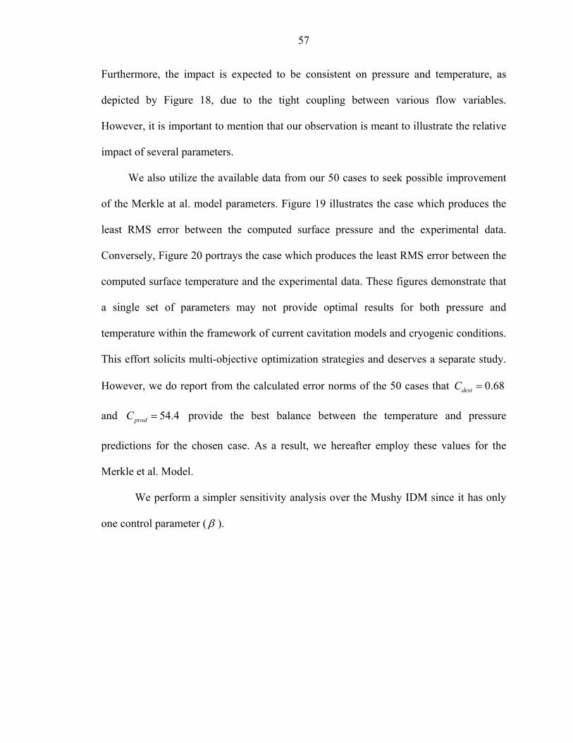
57
Furthermore, the impact is expected to be consistent on pressure and temperature, as
depicted by Figure 18, due to the tight coupling between various flow variables.
However, it is important to mention that our observation is meant to illustrate the relative
impact of several parameters.
We also utilize the available data from our 50 cases to seek possible improvement
of the Merkle at al. model parameters. Figure 19 illustrates the case which produces the
least RMS error between the computed surface pressure and the experimental data.
Conversely, Figure 20 portrays the case which produces the least RMS error between the
computed surface temperature and the experimental data. These figures demonstrate that
a single set of parameters may not provide optimal results for both pressure and
temperature within the framework of current cavitation models and cryogenic conditions.
This effort solicits multi-objective optimization strategies and deserves a separate study.
However, we do report from the calculated error norms of the 50 cases that 0.68destC =
and 54.4prodC = provide the best balance between the temperature and pressure
predictions for the chosen case. As a result, we hereafter employ these values for the
Merkle et al. Model.
We perform a simpler sensitivity analysis over the Mushy IDM since it has only
one control parameter (β ).
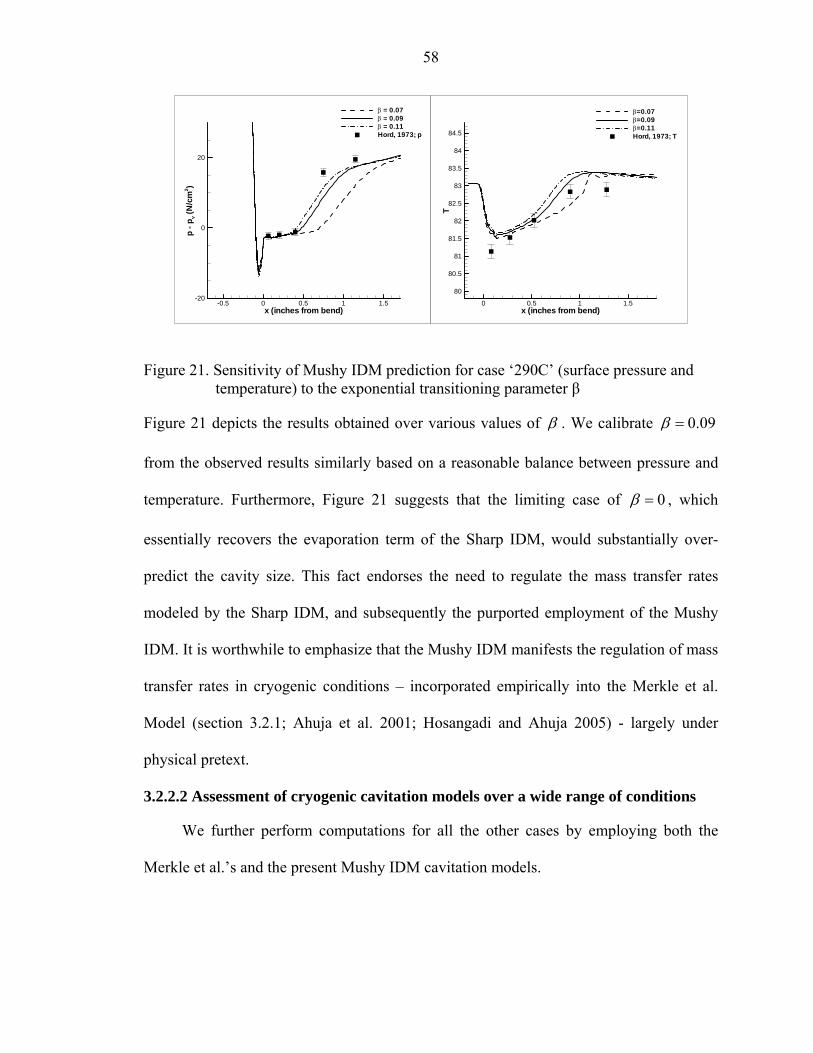
58
x (inches from bend)
p-p
v(N
/cm
2 )
-0.5 0 0.5 1 1.5-20
0
20
β = 0.07β = 0.09β = 0.11Hord, 1973; p
x (inches from bend)
T
0 0.5 1 1.5
80
80.5
81
81.5
82
82.5
83
83.5
84
84.5
β=0.07β=0.09β=0.11Hord, 1973; T
Figure 21. Sensitivity of Mushy IDM prediction for case ‘290C’ (surface pressure and temperature) to the exponential transitioning parameter β
Figure 21 depicts the results obtained over various values of β . We calibrate 0.09=β
from the observed results similarly based on a reasonable balance between pressure and
temperature. Furthermore, Figure 21 suggests that the limiting case of 0β = , which
essentially recovers the evaporation term of the Sharp IDM, would substantially over-
predict the cavity size. This fact endorses the need to regulate the mass transfer rates
modeled by the Sharp IDM, and subsequently the purported employment of the Mushy
IDM. It is worthwhile to emphasize that the Mushy IDM manifests the regulation of mass
transfer rates in cryogenic conditions – incorporated empirically into the Merkle et al.
Model (section 3.2.1; Ahuja et al. 2001; Hosangadi and Ahuja 2005) - largely under
physical pretext.
3.2.2.2 Assessment of cryogenic cavitation models over a wide range of conditions
We further perform computations for all the other cases by employing both the
Merkle et al.’s and the present Mushy IDM cavitation models.
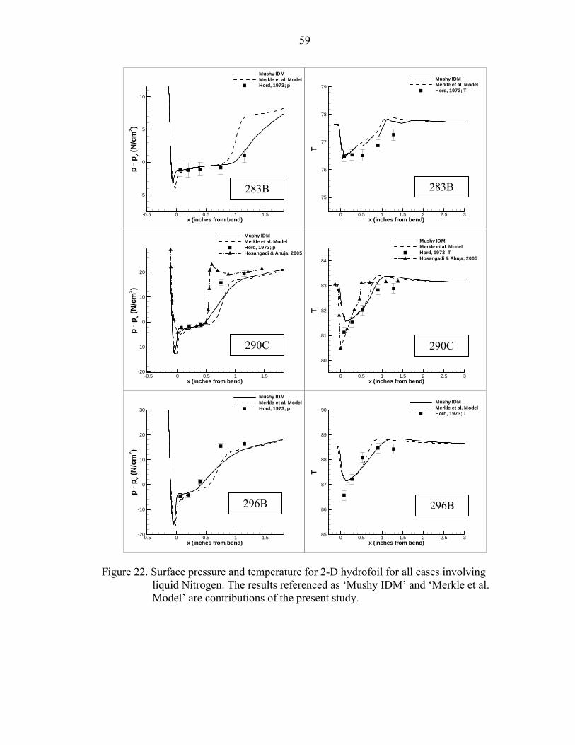
59
x (inches from bend)
p-p
v(N
/cm
2 )
-0.5 0 0.5 1 1.5
-5
0
5
10
Mushy IDMMerkle et al. ModelHord, 1973; p
x (inches from bend)
T
0 0.5 1 1.5 2 2.5 3
75
76
77
78
79
Mushy IDMMerkle et al. ModelHord, 1973; T
x (inches from bend)
p-p
v(N
/cm
2 )
-0.5 0 0.5 1 1.5-20
-10
0
10
20
Mushy IDMMerkle et al. ModelHord, 1973; pHosangadi & Ahuja, 2005
x (inches from bend)
T
0 0.5 1 1.5 2 2.5 3
80
81
82
83
84
Mushy IDMMerkle et al. ModelHord, 1973; THosangadi & Ahuja, 2005
x (inches from bend)
p-p
v(N
/cm
2 )
-0.5 0 0.5 1 1.5-20
-10
0
10
20
30
Mushy IDMMerkle et al. ModelHord, 1973; p
x (inches from bend)
T
0 0.5 1 1.5 2 2.5 385
86
87
88
89
90
Mushy IDMMerkle et al. ModelHord, 1973; T
Figure 22. Surface pressure and temperature for 2-D hydrofoil for all cases involving liquid Nitrogen. The results referenced as ‘Mushy IDM’ and ‘Merkle et al. Model’ are contributions of the present study.
283B 283B
290C 290C
296B 296B
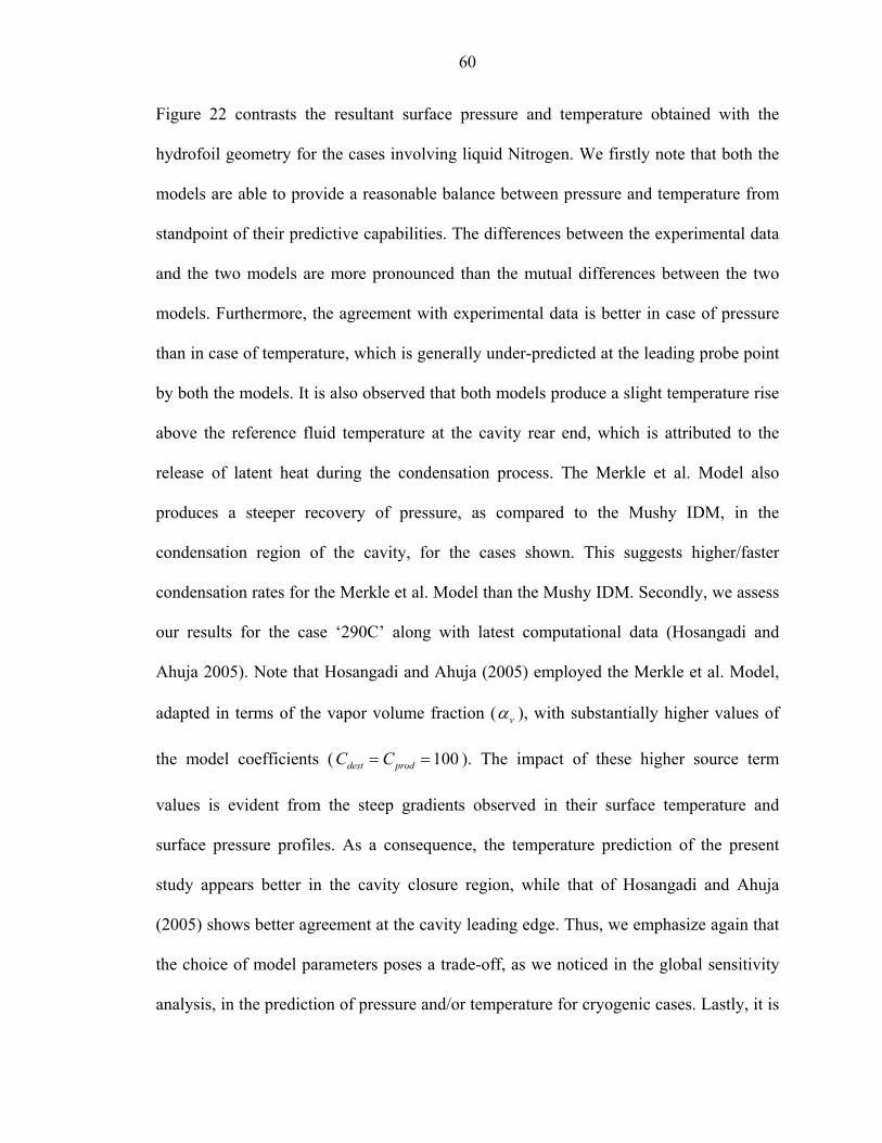
60
Figure 22 contrasts the resultant surface pressure and temperature obtained with the
hydrofoil geometry for the cases involving liquid Nitrogen. We firstly note that both the
models are able to provide a reasonable balance between pressure and temperature from
standpoint of their predictive capabilities. The differences between the experimental data
and the two models are more pronounced than the mutual differences between the two
models. Furthermore, the agreement with experimental data is better in case of pressure
than in case of temperature, which is generally under-predicted at the leading probe point
by both the models. It is also observed that both models produce a slight temperature rise
above the reference fluid temperature at the cavity rear end, which is attributed to the
release of latent heat during the condensation process. The Merkle et al. Model also
produces a steeper recovery of pressure, as compared to the Mushy IDM, in the
condensation region of the cavity, for the cases shown. This suggests higher/faster
condensation rates for the Merkle et al. Model than the Mushy IDM. Secondly, we assess
our results for the case ‘290C’ along with latest computational data (Hosangadi and
Ahuja 2005). Note that Hosangadi and Ahuja (2005) employed the Merkle et al. Model,
adapted in terms of the vapor volume fraction ( vα ), with substantially higher values of
the model coefficients ( 100dest prodC C= = ). The impact of these higher source term
values is evident from the steep gradients observed in their surface temperature and
surface pressure profiles. As a consequence, the temperature prediction of the present
study appears better in the cavity closure region, while that of Hosangadi and Ahuja
(2005) shows better agreement at the cavity leading edge. Thus, we emphasize again that
the choice of model parameters poses a trade-off, as we noticed in the global sensitivity
analysis, in the prediction of pressure and/or temperature for cryogenic cases. Lastly, it is
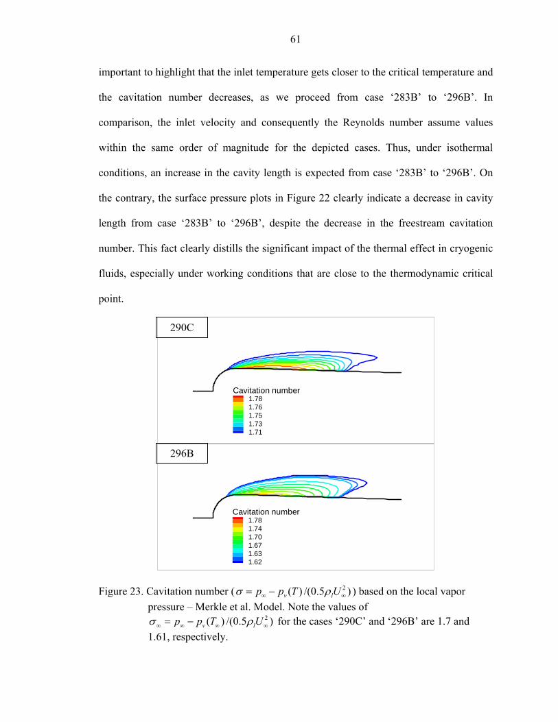
61
important to highlight that the inlet temperature gets closer to the critical temperature and
the cavitation number decreases, as we proceed from case ‘283B’ to ‘296B’. In
comparison, the inlet velocity and consequently the Reynolds number assume values
within the same order of magnitude for the depicted cases. Thus, under isothermal
conditions, an increase in the cavity length is expected from case ‘283B’ to ‘296B’. On
the contrary, the surface pressure plots in Figure 22 clearly indicate a decrease in cavity
length from case ‘283B’ to ‘296B’, despite the decrease in the freestream cavitation
number. This fact clearly distills the significant impact of the thermal effect in cryogenic
fluids, especially under working conditions that are close to the thermodynamic critical
point.
Cavitation number1.781.761.751.731.71
Cavitation number1.781.741.701.671.631.62
Figure 23. Cavitation number ( 2( ) /(0.5 )v lp p T Uσ ρ∞ ∞= − ) based on the local vapor
pressure – Merkle et al. Model. Note the values of 2( ) /(0.5 )v lp p T Uσ ρ∞ ∞ ∞ ∞= − for the cases ‘290C’ and ‘296B’ are 1.7 and
1.61, respectively.
296B
290C
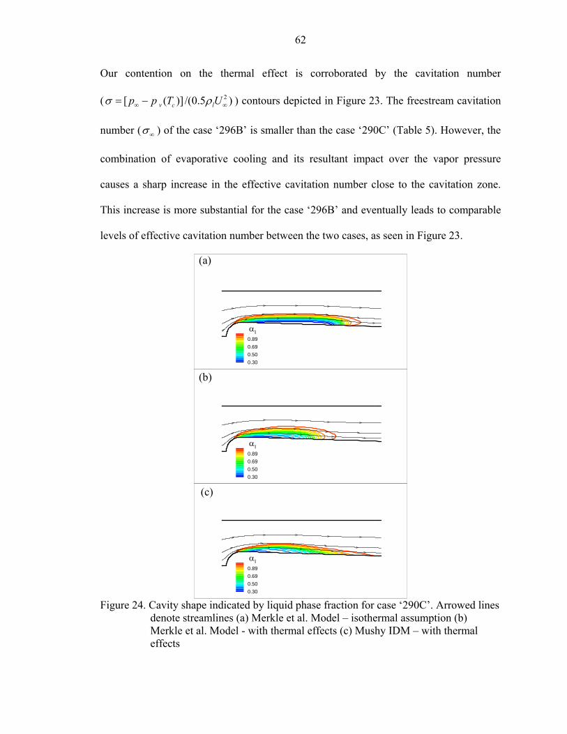
62
Our contention on the thermal effect is corroborated by the cavitation number
( 2[ ( )] /(0.5 )v c lp p T Uσ ρ∞ ∞= − ) contours depicted in Figure 23. The freestream cavitation
number (σ∞ ) of the case ‘296B’ is smaller than the case ‘290C’ (Table 5). However, the
combination of evaporative cooling and its resultant impact over the vapor pressure
causes a sharp increase in the effective cavitation number close to the cavitation zone.
This increase is more substantial for the case ‘296B’ and eventually leads to comparable
levels of effective cavitation number between the two cases, as seen in Figure 23.
αl0.890.690.500.30
αl0.890.690.500.30
αl0.890.690.500.30
Figure 24. Cavity shape indicated by liquid phase fraction for case ‘290C’. Arrowed lines denote streamlines (a) Merkle et al. Model – isothermal assumption (b) Merkle et al. Model - with thermal effects (c) Mushy IDM – with thermal effects
(a)
(b)
(c)
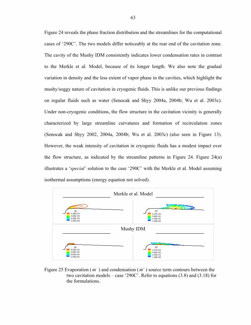
63
Figure 24 reveals the phase fraction distribution and the streamlines for the computational
cases of ‘290C’. The two models differ noticeably at the rear end of the cavitation zone.
The cavity of the Mushy IDM consistently indicates lower condensation rates in contrast
to the Merkle et al. Model, because of its longer length. We also note the gradual
variation in density and the less extent of vapor phase in the cavities, which highlight the
mushy/soggy nature of cavitation in cryogenic fluids. This is unlike our previous findings
on regular fluids such as water (Senocak and Shyy 2004a, 2004b; Wu et al. 2003c).
Under non-cryogenic conditions, the flow structure in the cavitation vicinity is generally
characterized by large streamline curvatures and formation of recirculation zones
(Senocak and Shyy 2002, 2004a, 2004b; Wu et al. 2003c) (also seen in Figure 13).
However, the weak intensity of cavitation in cryogenic fluids has a modest impact over
the flow structure, as indicated by the streamline patterns in Figure 24. Figure 24(a)
illustrates a ‘special’ solution to the case ‘290C’ with the Merkle et al. Model assuming
isothermal assumptions (energy equation not solved).
m-
-5.36E+02-3.69E+03-6.85E+03-1.00E+04
m+
2.37E+033.95E+022.50E+011.36E+00
m-
-5.36E+02-3.69E+03-6.85E+03-1.00E+04
m+
2.37E+033.95E+022.50E+011.36E+00
Figure 25 Evaporation ( m−& ) and condensation ( m+& ) source term contours between the
two cavitation models – case ‘290C’. Refer to equations (3.8) and (3.18) for the formulations.
Merkle et al. Model
Mushy IDM
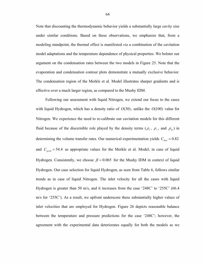
64
Note that discounting the thermodynamic behavior yields a substantially large cavity size
under similar conditions. Based on these observations, we emphasize that, from a
modeling standpoint, the thermal effect is manifested via a combination of the cavitation
model adaptations and the temperature dependence of physical properties. We bolster our
argument on the condensation rates between the two models in Figure 25. Note that the
evaporation and condensation contour plots demonstrate a mutually exclusive behavior.
The condensation region of the Merkle et al. Model illustrates sharper gradients and is
effective over a much larger region, as compared to the Mushy IDM.
Following our assessment with liquid Nitrogen, we extend our focus to the cases
with liquid Hydrogen, which has a density ratio of (30)O , unlike the (100)O value for
Nitrogen. We experience the need to re-calibrate our cavitation models for this different
fluid because of the discernible role played by the density terms ( lρ , vρ , and mρ ) in
determining the volume transfer rates. Our numerical experimentation yields 0.82destC =
and 54.4prodC = as appropriate values for the Merkle et al. Model, in case of liquid
Hydrogen. Consistently, we choose 0.065β = for the Mushy IDM in context of liquid
Hydrogen. Our case selection for liquid Hydrogen, as seen from Table 6, follows similar
trends as in case of liquid Nitrogen. The inlet velocity for all the cases with liquid
Hydrogen is greater than 50 m/s, and it increases from the case ‘248C’ to ‘255C’ (66.4
m/s for ‘255C’). As a result, we upfront underscore these substantially higher values of
inlet velocities that are employed for Hydrogen. Figure 26 depicts reasonable balance
between the temperature and pressure predictions for the case ‘248C’; however, the
agreement with the experimental data deteriorates equally for both the models as we
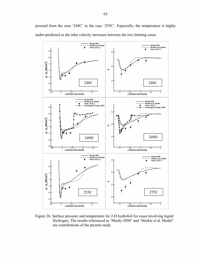
65
proceed from the case ‘248C’ to the case ‘255C’. Especially, the temperature is highly
under-predicted as the inlet velocity increases between the two limiting cases.
x (inches from bend)
p-p
v(N
/cm
2 )
-0.5 0 0.5 1 1.5-15
-10
-5
0
5
10
15
Mushy IDMMerkle et al. ModelHord, 1973; p
x (inches from bend)
T
0 0.5 1 1.5 2
19
20
21
Mushy IDMMerkle et al. ModelHord, 1973; T
x (inches from bend)
p-p
v(N
/cm
2 )
-0.5 0 0.5 1 1.5-15
-10
-5
0
5
10
15
Mushy IDMMerkle et al. ModelHord, 1973; pHosangadi & Ahuja, 2005
x (inches from bend)
T
0 0.5 1 1.5 2
19
20
21
Mushy IDMMerkle et al. ModelHord, 1973; THosangadi & Ahuja, 2005
x (inches from bend)
p-p
v(N
/cm
2 )
-0.5 0 0.5 1 1.5
-15
-10
-5
0
5
10
Mushy IDMMerkle et al. ModelHord, 1973; p
x (inches from bend)
T
0 0.5 1 1.5 2
20
21
22
23
Mushy IDMMerkle et al. ModelHord, 1973; T
Figure 26. Surface pressure and temperature for 2-D hydrofoil for cases involving liquid Hydrogen. The results referenced as ‘Mushy IDM’ and ‘Merkle et al. Model’ are contributions of the present study.
249D 249D
255C 255C
248C 248C
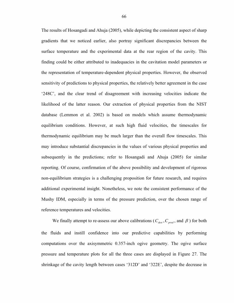
66
The results of Hosangadi and Ahuja (2005), while depicting the consistent aspect of sharp
gradients that we noticed earlier, also portray significant discrepancies between the
surface temperature and the experimental data at the rear region of the cavity. This
finding could be either attributed to inadequacies in the cavitation model parameters or
the representation of temperature-dependent physical properties. However, the observed
sensitivity of predictions to physical properties, the relatively better agreement in the case
‘248C’, and the clear trend of disagreement with increasing velocities indicate the
likelihood of the latter reason. Our extraction of physical properties from the NIST
database (Lemmon et al. 2002) is based on models which assume thermodynamic
equilibrium conditions. However, at such high fluid velocities, the timescales for
thermodynamic equilibrium may be much larger than the overall flow timescales. This
may introduce substantial discrepancies in the values of various physical properties and
subsequently in the predictions; refer to Hosangadi and Ahuja (2005) for similar
reporting. Of course, confirmation of the above possibility and development of rigorous
non-equilibrium strategies is a challenging proposition for future research, and requires
additional experimental insight. Nonetheless, we note the consistent performance of the
Mushy IDM, especially in terms of the pressure prediction, over the chosen range of
reference temperatures and velocities.
We finally attempt to re-assess our above calibrations ( destC , prodC , and β ) for both
the fluids and instill confidence into our predictive capabilities by performing
computations over the axisymmetric 0.357-inch ogive geometry. The ogive surface
pressure and temperature plots for all the three cases are displayed in Figure 27. The
shrinkage of the cavity length between cases ‘312D’ and ‘322E’, despite the decrease in
67
the reference cavitation number, unequivocally re-emphasizes the influence of the
thermo-sensible working conditions.
x in inches from bend
p-p
v(N
/cm
2 )
0 0.5 1 1.5-10
-5
0
5
10
15
20
Mushy IDMMerkle et al. ModelHord, 1973; p
x in inches from bend
Tin
K
0 0.5 1 1.580
81
82
83
84
Mushy IDMMerkle et al. ModelHord, 1973; T
x in inches from bend
p-p
v(N
/cm
2 )
0 0.2 0.4 0.6 0.8 1 1.2 1.4-15
-10
-5
0
5
10
15
20
25
Mushy IDMMerkle et al. ModelHord, 1973; p
x in inches from bend
Tin
K
0 0.5 1 1.585
86
87
88
89
90
Mushy IDMMerkle et al. ModelHord, 1973; T
x in inches from bend
p-p
v(N
/cm
2 )
0 0.2 0.4 0.6 0.8 1 1.2 1.4-15
-10
-5
0
5
10
15
20
25
Mushy IDMMerkle et al. ModelHord, 1973; p
x in inches from bend
Tin
K
0 0.5 1 1.519
19.5
20
20.5
21
21.5
22
Mushy IDMMerkle et al. ModelHord, 1973; T
Figure 27. Surface pressure and temperature for axisymmetric ogive for all the cases (Nitrogen and Hydrogen). The results referenced as ‘Mushy IDM’ and ‘Merkle et al. Model’ are contributions of the present study.
312D 312D
322E 322E
349B 349B
68
Furthermore, the discrepancy in our predictions for liquid Hydrogen, when subjected to
higher velocities, is also evidenced by the plots for the case ‘349B’. Overall, the
agreement with experimental data in all the cases is better in terms of the surface pressure
than temperature. But, unlike the hydrofoil geometry, the temperature at the first
(leading) probe point is over-predicted for all the ogive cases. As expected, this
discrepancy is most in the liquid Hydrogen case (‘349B’). Thus, the two geometries do
not produce a consistent pattern of disagreement midst the surface temperature and the
experimental measurements. This inconsistent behavior warrants further experimental
and numerical probing from a standpoint of developing more precise cavitation models
for cryogenic cavitation. Nonetheless, we observe that our analyses/calibrations are able
to yield a justifiable range of results for the ogive geometry as well.
69
CHAPTER 4 TIME-DEPENDENT COMPUTATIONS FOR FLOWS INVOLVING PHASE
CHANGE
Researchers have striven to develop efficient and accurate methodologies to
simulate time-dependent cavitating flows. The multiphase nature of the flow
accompanied by complex flow physics yields a system of tightly-coupled governing
equations. Furthermore, interfacial dynamics, compressibility effects in mixture region,
and turbulence entail deployment of numerical models to represent these physical
phenomena. The formulation of these models substantially impacts the solution
procedure. As a result, evolving efficient algorithms for unsteady cavitating flows is
certainly a non-trivial task.
Formulation of implicit procedures for pressure-based methods is impeded mainly
by the strong linkage between the flow variables such as velocity and pressure.
Furthermore, the dynamics of the variable density field in cavitating flows imposes
supplementary equations on the existing system, which add to the computational
challenges. As a result, iterative algorithms such as SIMPLE, SIMPLER, and SIMPLEC
(Versteeg and Malalasekera 1995), which are commonly employed for a wide variety of
problems, may be computationally expensive for solution of cavitating flows with
pronounced unsteady behavior. Senocak and Shyy (2002, 2004b) circumvented this
difficulty by incorporating the Pressure Implicit with Splitting of Operators (PISO)
algorithm suitably with the model equation of cavitation dynamics and the sound
propagation model for the mixture region. This endeavor resulted in a non-iterative
70
methodology for time-dependent computation of cavitating flow through a series of
predictor-corrector steps. Senocak and Shyy (2002, 2004b) demonstrated the merits of
this efficient approach with a series of cavitating flow computations on geometries such
as Convergent-Divergent Nozzle and hemispherical solids.
However, all the past efforts were in the context of isothermal cavitation sans the
energy implications and real fluid properties. From standpoint of formulating a non-
iterative algorithm for cryogenic cases, the inclusion of the non-linear energy equation
and temperature dependence of physical properties into the existing methodology is
expected to pose multitude of adversities to the solution efficiency and accuracy. Direct
development of an algorithm for cryogenic cavitation may be a presumptuous
preliminary approach. As a result, we initiate a multiphase non-iterative procedure on a
simpler test problem with similar nature of challenges, and, with an objective of
monitoring the accuracy and stability of the computations.
In this chapter, we elucidate the newly initiated algorithm and illustrate its results
on a chosen test case. The truly unsteady problem of Gallium fusion (with natural
convection effects) is adopted for the purpose of validation. Discussion on the grid
sensitivity, accuracy of results, and the stability criterion is provided. The above primary
objective is complimented by a reduced-order description of the gallium fusion problem
by Proper Orthogonal Decomposition (POD). The flowfield in the problem is
characterized by a solid-liquid front movement with a continuous change in the overall
flow length scale. The ability of POD, to accommodate these varying flow scales, is
mainly emphasized.
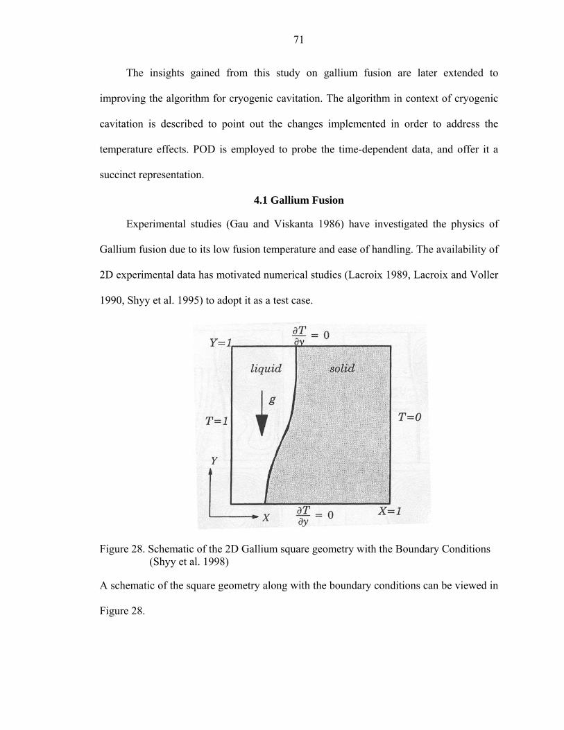
71
The insights gained from this study on gallium fusion are later extended to
improving the algorithm for cryogenic cavitation. The algorithm in context of cryogenic
cavitation is described to point out the changes implemented in order to address the
temperature effects. POD is employed to probe the time-dependent data, and offer it a
succinct representation.
4.1 Gallium Fusion
Experimental studies (Gau and Viskanta 1986) have investigated the physics of
Gallium fusion due to its low fusion temperature and ease of handling. The availability of
2D experimental data has motivated numerical studies (Lacroix 1989, Lacroix and Voller
1990, Shyy et al. 1995) to adopt it as a test case.
Figure 28. Schematic of the 2D Gallium square geometry with the Boundary Conditions (Shyy et al. 1998)
A schematic of the square geometry along with the boundary conditions can be viewed in
Figure 28.
72
4.1.1 Governing Equations
The single-fluid modeling approach is adopted by employing a liquid phase
fraction f. The density is assumed constant through the Buossinesq approximation. The
governing equations for the problem are as follows.
0i
i
ux∂
=∂
(4.1)
2
0 23
( )( ) 1( ) ( ) ( )j ii ii i
j i j j
u uu up fC u g T Tt x x x x f q
ρρ µ ρβ δ∂∂ ∂∂ ∂ −
+ = − + − + −∂ ∂ ∂ ∂ ∂ +
(4.2)
( ) ( ) ( )jj j j
h Tu h kt x x xρ ρ∂ ∂ ∂ ∂
+ =∂ ∂ ∂ ∂
(4.3)
Here, β represents the coefficient of thermal expansion for the fluid. The term
2
3
1( ) ifC u
f q−+
in the momentum equations is the Darcy source term (Shyy et al. 1998).
Through their functional dependence on f, they are modeled to retard the velocity to
insignificant values in solid region. The constants C and q, in compliance, are tuned to
yield a negative source term, which is at least seven orders of magnitude higher than
other terms, in the solid region (f = 0). The enthalpy in equation (4.3) is expressed as:
Ph C T fL= + (4.4)
The phase fraction f is modeled computationally by the h-based method (Shyy et al.
1998). The enthalpy at any given iteration is computed as shown below followed by an
update of f (explained in a later section).
1k k kPh C T f L−= + (4.5)
Note that f is always bounded by 0 and 1. Thus, equation (4.5) can be recast into a
temperature equation as shown.
73
( ) ( )( ) ( ) [ ( )]PP j j
j j j j
C T T LfC u T k Lu ft x x x t x
ρ ρρ ρ∂ ∂ ∂ ∂ ∂ ∂+ = − +
∂ ∂ ∂ ∂ ∂ ∂ (4.6)
The iterative update of the liquid phase fraction, as mentioned above, renders the
energy/temperature equation non-linear. Furthermore, the buoyancy term in equation
(4.2) leads to a pressure-velocity-temperature coupling. The non-linearity in the energy
equation and the strong coupling between various flow variables justify the use of the
gallium fusion problem as a test case preceding the cryogenic problem. The physical
properties such as viscosity, latent heat, thermal conductivity, and specific heat are,
however, assumed to be constant during the fusion process.
4.1.2 Numerical Algorithm
The previous computations on similar multiphase problems employed an iterative
solution strategy (Chuan et al. 1991, Khodadadi and Zhang 2001). Conversely, the PISO
method (Issa 1985, Thakur et al. 2002, Thakur and Wright 2004), which forms the
backbone of the current algorithm, essentially is a series of predictor corrector steps to
yield a non-iterative solution of flow equations through operator splitting procedure. The
present methodology, however, closely follows a slightly modified version of PISO
designed for buoyancy driven single-phase flows (Oliveira and Issa 2001). Kim et al.
(2000) proposed a series of steps to accelerate the simple heat conduction equation with a
solid-liquid phase boundary. The following methodology attempts to blend the merits of
the modified PISO (Oliveira and Issa 2001) with the propositions of Kim et al. (2000), to
design an efficient and accurate algorithm for phase change problems. The sequence of
calculations for the algorithm, based on the above governing equations, is expounded
below.
74
The strongly implicit form of the discretized governing equations with a finite
volume formulation, at any node P, is as follows:
1
1 1 1 1
1 1 1 1
1
1 1 1
( ) 0
( ) ( )
( ) ( )
( )
( ) ( )
ni i
u n u n n u n u nP P nb nb u p P P
v n v n n v n v nP P nb nb v p P P
v nP
T n T n T n f n nP P nb nb P P P P
u
A u A u p H u S u
A v A v p H v S v
B T
A T A T H T H f M f
ρ +
+ + + +
+ + + +
+
+ + +
∆ =
= −∆ + +
= − ∆ + +
+
= + + +
∑∑
∑
(4.7)
Here, A represents the terms at the current time level, H represents the terms at older time
step, M represents the terms involving the phase fraction f, B represents the buoyancy
term, and S represents the Darcy source term. The Darcy source terms can be absorbed
into the left hand side term to yield to following equations.
1
1 1 1
1 1 1 1
1 1 1
( ) 0
( )
( ) ( )
( ) ( )
ni i
u n u n n u nP P nb nb u p P
v n v n n v n v nP P nb nb v p P P
T n T n T n f n nP P nb nb P P P P
u
G u A u p H u
G v A v p H v B T
A T A T H T H f M f
ρ +
+ + +
+ + + +
+ + +
∆ =
= − ∆ +
= −∆ + +
= + + +
∑∑∑
(4.8)
Here, u u uP P PG A S= + and so on. The sequence of steps to solve equation (4.8) non-
iteratively is elaborated next.
(a) Momentum predictor
* *
* *
( )
( ) ( )
u u n u nP P nb nb u p P
v v n v n v nP P nb nb v p P P
G u A u p H u
G v A v p H v B T
= −∆ +
= −∆ + +
∑∑
(4.9)
These velocities - *u and *v - are obtained by using the pressure value at the previous
time step and hence are not divergence free.
75
(b) First pressure corrector
**
*
( ) 0
( ') ( )i
i i
i i i iuP
u
p uG
ρρ ρ
∆ =
∆ ∆ = ∆ (4.10)
Here, *'p p p= − is calculated. The pressure field *p can now be employed for
correcting the divergence error in velocity. Note that the pressure correction at this stage
is limited by several approximations and is not adequate to produce an accurate velocity
field.
(c) First momentum corrector
** * *
** * *
( )
( ) ( )
u u u nP P nb nb u p P
v v v n nP P nb nb v p P v
G u A u p H u
G v A v p H v B T
= −∆ +
= −∆ + +
∑∑
(4.11)
The velocities are corrected to yield **u and **v explicitly using the intermediate pressure
field obtained in the previous step.
(d) First temperature corrector
* * *( ) ( )T T T n f nP P nb nb P P P PA T A T H T H f M f= + + +∑ (4.12)
The above temperature equation utilizes the latest value of f. However, in view of a non-
iterative strategy, solution of temperature, merely by the above equation, may not be
sufficient for rapid convergence due to the delayed update of f. As a remedy, a series of
explicit steps are implemented following the above equation to significantly improve the
prediction of temperature and, subsequently, f. These steps are adapted from the
algorithm proposed by Kim et al. (2000) for pure conduction equation. They are enlisted
below.
(i) Update f by h-based method as shown.
76
1 1
1 1
1 1
11
0 if
1 if
elsewhere
where, ,
k k kP P P Pk k
P p s
k kP p l
kk P s
Pl s
s P m l P m
h C T f L
f h h
f h h
h hfh hh C T h C T L
+ +
+ +
+ +
++
= +
= <
= >
−=
−= = +
(4.13)
Note that at the outset 1 *kP PT T+ = .
(ii) If 1k kP Pf f+ ≠ , correct temperature using the explicit form of equation (4.12)
with updated coefficients. This step yields the new temperature field 2kPT + .
(iii) Compute residual of the temperature equation as shown further.
2 2 1( ) ( )T k T k T n f n kP P nb nb P P P PA T A T H T H f M f+ + +Φ = − + + +∑ (4.14)
The above residual equation can be further employed to improve temperature
prediction by Newton-Raphson approach as follows (Kim et al. 2000):
3 2
2
k kP p
kP
T T
T
+ +
+
Φ= −
∂Φ∂
(4.15)
where, the Jacobian is approximated as 2TPk
p
AT +
∂Φ≈
∂.
In summary, steps (i) – (iii) are performed at least 10-12 times following the equation
(4.12). Let the temperature and phase fraction field at the end of this stage be denoted as
* * and T f .
77
(e) Second pressure corrector
***
** *
** *
* **
( ) 0
( ") ( ( ) ( )
[( ) ( )] )
i i
i i
v v ni i i P Pu u
P Pi inb nb
i iP P P
u
p B T B TG G
A u A u
S S u
ρρ ρ
∆ =
∆ ∆ = ∆ − +
− −
−∑ ∑
(4.16)
This step is a powerful characteristic of the PISO algorithm. The ‘differential Darcy
term’, * **( ) ( )i iP P PS S u− , is an addition to the terms already suggested by Issa (1985) and
Oliveira and Issa (2001). This term arises out of the update of iuPG after the first
temperature corrector. Note that the coefficient iuPG , unlike single-phase flow cases, also
includes the implicit coefficient of the Darcy term (refer to the discussion in step (a)).
The Darcy term undergoes a sudden change over several orders of magnitude between
the liquid and the solid region. Since the first temperature corrector tends to change the
phase fraction distribution, it is imperative to update the coefficient iuPG post that step.
The second pressure corrector, which is obtained via subtracting equation (4.11) from
(4.17), is thus able to account for phase front movement because of the ‘differential
Darcy term’. In summary, the second pressure corrector attempts to couple the non-linear
terms in the momentum equations, the temperature field, and the phase front movement
to the pressure field.
(f) Second momentum corrector
* *** ** **
* *** ** ** *
( )
( ) ( )
u u u np P nb nb u p P
v v v n vp P nb nb v p P P
G u A u p H u
G v A v p H v B T
= −∆ +
= −∆ + +
∑∑
(4.17)
The velocity field at this stage is derived from the more accurate prediction of pressure
**p obtained from the previous step.
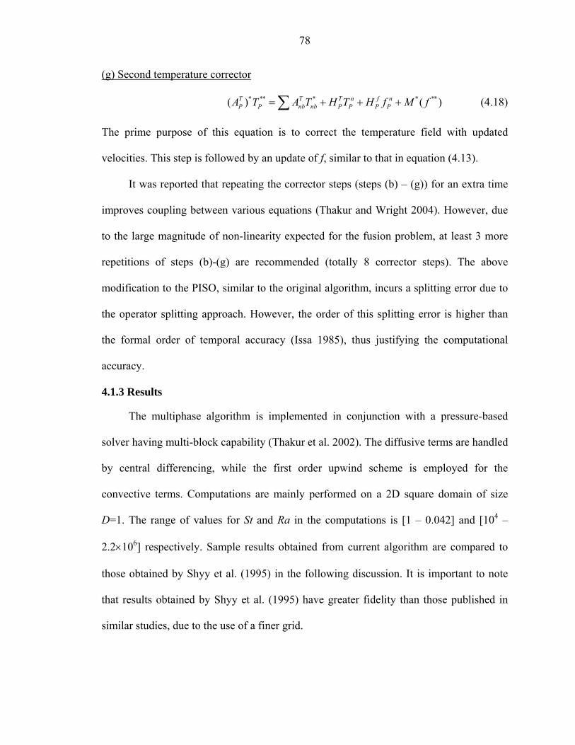
78
(g) Second temperature corrector
* ** * * **( ) ( )T T T n f nP P nb nb P P P PA T A T H T H f M f= + + +∑ (4.18)
The prime purpose of this equation is to correct the temperature field with updated
velocities. This step is followed by an update of f, similar to that in equation (4.13).
It was reported that repeating the corrector steps (steps (b) – (g)) for an extra time
improves coupling between various equations (Thakur and Wright 2004). However, due
to the large magnitude of non-linearity expected for the fusion problem, at least 3 more
repetitions of steps (b)-(g) are recommended (totally 8 corrector steps). The above
modification to the PISO, similar to the original algorithm, incurs a splitting error due to
the operator splitting approach. However, the order of this splitting error is higher than
the formal order of temporal accuracy (Issa 1985), thus justifying the computational
accuracy.
4.1.3 Results
The multiphase algorithm is implemented in conjunction with a pressure-based
solver having multi-block capability (Thakur et al. 2002). The diffusive terms are handled
by central differencing, while the first order upwind scheme is employed for the
convective terms. Computations are mainly performed on a 2D square domain of size
D=1. The range of values for St and Ra in the computations is [1 – 0.042] and [104 –
2.2×10⁶] respectively. Sample results obtained from current algorithm are compared to
those obtained by Shyy et al. (1995) in the following discussion. It is important to note
that results obtained by Shyy et al. (1995) have greater fidelity than those published in
similar studies, due to the use of a finer grid.

79
4.1.3.1 Accuracy and grid dependence
X
Y
0 0.5 10
0.2
0.4
0.6
0.8
1
X
Y
0 0.5 10
0.2
0.4
0.6
0.8
1
X
Y
0 0.5 10
0.2
0.4
0.6
0.8
1
X
Y
0 0.5 10
0.2
0.4
0.6
0.8
1
X
Y
0 0.5 10
0.2
0.4
0.6
0.8
1
X
Y
0 0.5 10
0.2
0.4
0.6
0.8
1
X
Y
0 0.5 10
0.2
0.4
0.6
0.8
1
X
Y
0 0.5 10
0.2
0.4
0.6
0.8
1
X
Y
0 0.5 10
0.2
0.4
0.6
0.8
1
Figure 29. 2D interface location at various instants for St = 0.042, Ra = 2.2 × 10⁵ and Pr = 0.0208. White circles represent interface locations obtained by Shyy et al. (1995) on a 41×41 grid at time instants at t = 56.7s, 141.8s, & 227s respectively.
Figure 29 illustrates the 2D interface locations obtained with the current algorithm,
with three different grid resolutions, for the parameters shown. Note that some results by
Shyy et al. (1995) are at a slightly earlier time instant. This contributes to the modest
difference observed in the interface location, especially during the early stages, when the
interface velocity is significantly higher. Considering this fact, the present results show
reasonable agreement with the earlier computation. Furthermore, the time-dependent
movement of the interface is consistent on all the three grids, although there is a
qualitative impact of the resolution on the interface profile.
21×21 grid
81×81 grid
41×41 grid
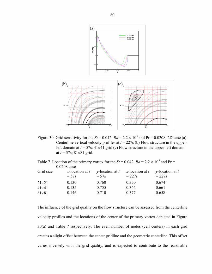
80
X
v(x,
0.5
)
0 0.25 0.5 0.75 1
-0.25
0
0.25
0.5
21x21 grid41x41 grid81x81 grid
X
Y
0 0.1 0.20.8
0.9
1
X
Y
0 0.1 0.20.8
0.9
1
Figure 30. Grid sensitivity for the St = 0.042, Ra = 2.2 × 10⁵ and Pr = 0.0208, 2D case (a) Centerline vertical velocity profiles at t = 227s (b) Flow structure in the upper-left domain at t = 57s; 41×41 grid (c) Flow structure in the upper-left domain at t = 57s; 81×81 grid.
Table 7. Location of the primary vortex for the St = 0.042, Ra = 2.2 × 10⁵ and Pr = 0.0208 case
Grid size x-location at t = 57s
y-location at t = 57s
x-location at t = 227s
y-location at t = 227s
21×21 0.130 0.760 0.350 0.674 41×41 0.135 0.755 0.365 0.661 81×81 0.146 0.710 0.377 0.658
The influence of the grid quality on the flow structure can be assessed from the centerline
velocity profiles and the locations of the center of the primary vortex depicted in Figure
30(a) and Table 7 respectively. The even number of nodes (cell centers) in each grid
creates a slight offset between the center gridline and the geometric centerline. This offset
varies inversely with the grid quality, and is expected to contribute to the reasonable
(a)
(c) (b)
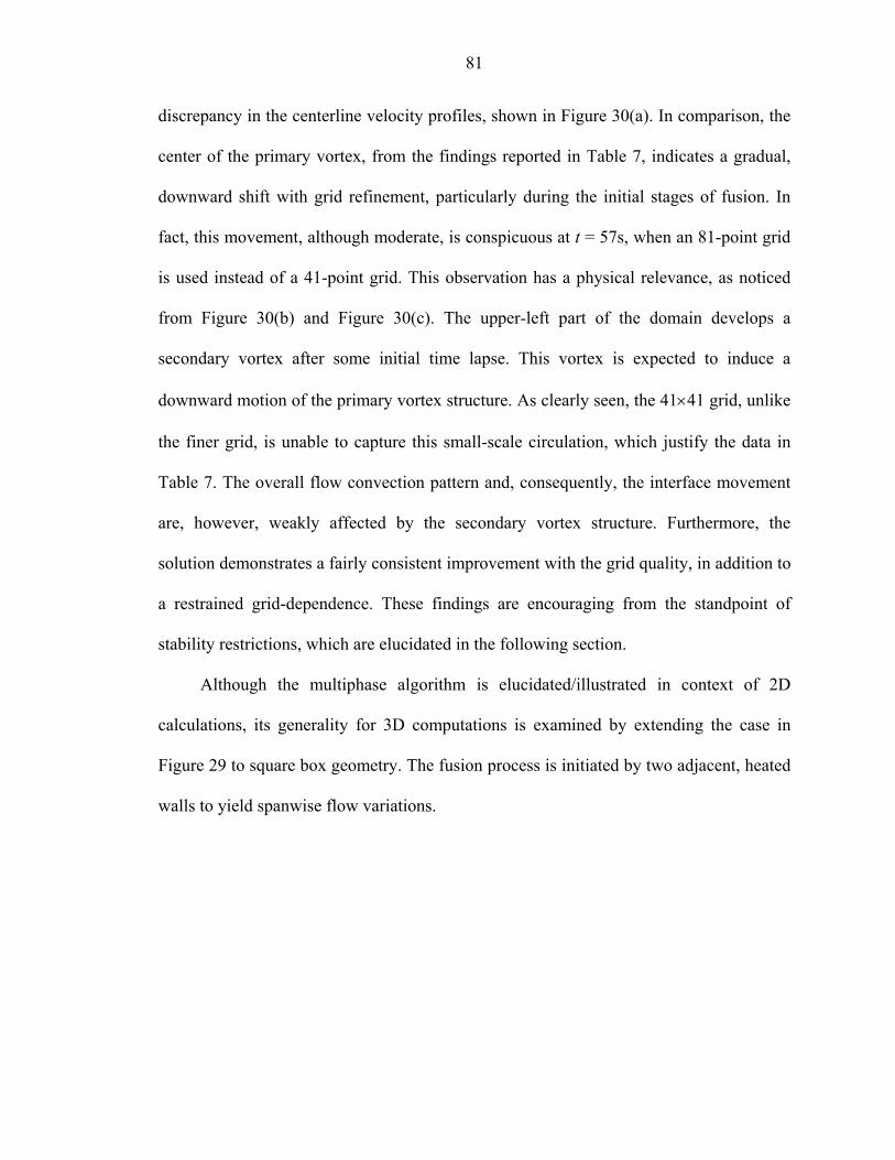
81
discrepancy in the centerline velocity profiles, shown in Figure 30(a). In comparison, the
center of the primary vortex, from the findings reported in Table 7, indicates a gradual,
downward shift with grid refinement, particularly during the initial stages of fusion. In
fact, this movement, although moderate, is conspicuous at t = 57s, when an 81-point grid
is used instead of a 41-point grid. This observation has a physical relevance, as noticed
from Figure 30(b) and Figure 30(c). The upper-left part of the domain develops a
secondary vortex after some initial time lapse. This vortex is expected to induce a
downward motion of the primary vortex structure. As clearly seen, the 41×41 grid, unlike
the finer grid, is unable to capture this small-scale circulation, which justify the data in
Table 7. The overall flow convection pattern and, consequently, the interface movement
are, however, weakly affected by the secondary vortex structure. Furthermore, the
solution demonstrates a fairly consistent improvement with the grid quality, in addition to
a restrained grid-dependence. These findings are encouraging from the standpoint of
stability restrictions, which are elucidated in the following section.
Although the multiphase algorithm is elucidated/illustrated in context of 2D
calculations, its generality for 3D computations is examined by extending the case in
Figure 29 to square box geometry. The fusion process is initiated by two adjacent, heated
walls to yield spanwise flow variations.
82
Figure 31. 3D interface location at t = 57s & 227s fo0.0208 case on a 41×41×41 grid. Top anT = 0; South and East: T = 1 (heated wal
X
Y
0 0.5 10
0.1
0.2
0.3
0.4
0.5
0.6
0.7
0.8
0.9
1z = 0.24
X
Y
0 0.50
0.1
0.2
0.3
0.4
0.5
0.6
0.7
0.8
0.9
1z = 0.5
Figure 32. Interface location and flow pattern for the
and Pr = 0.0208 case at various z locatio
Figure 31 and Figure 32 depict the interface movem
flow structure respectively. Note that the time-step s
41×41 2D grid. Accounting the dual heating su
consistent to those in Figure 29 and instill c
methodology.
4.1.3.2 Stability
As seen clearly, the basic framework of
corrector steps. As a result, the stable performance
inevitable restriction on the time-step size. N
Z
r St = 0.042, Ra = 2.2 × 10⁵ and Pr = d bottom: adiabatic; North and West: ls)
1X
Y
0 0.5 10
0.1
0.2
0.3
0.4
0.5
0.6
0.7
0.8
0.9
1z = 0.75
3D case, St = 0.042, Ra = 2.2 × 10⁵ ns, at t = 227s
ent and spanwise dependence of the
ize for the 3D case is equal to that for
rfaces, the results are qualitatively
onfidence in 3D capability of the
PISO incorporates several explicit
of the algorithm is restrained by an
umerical experimentation over the
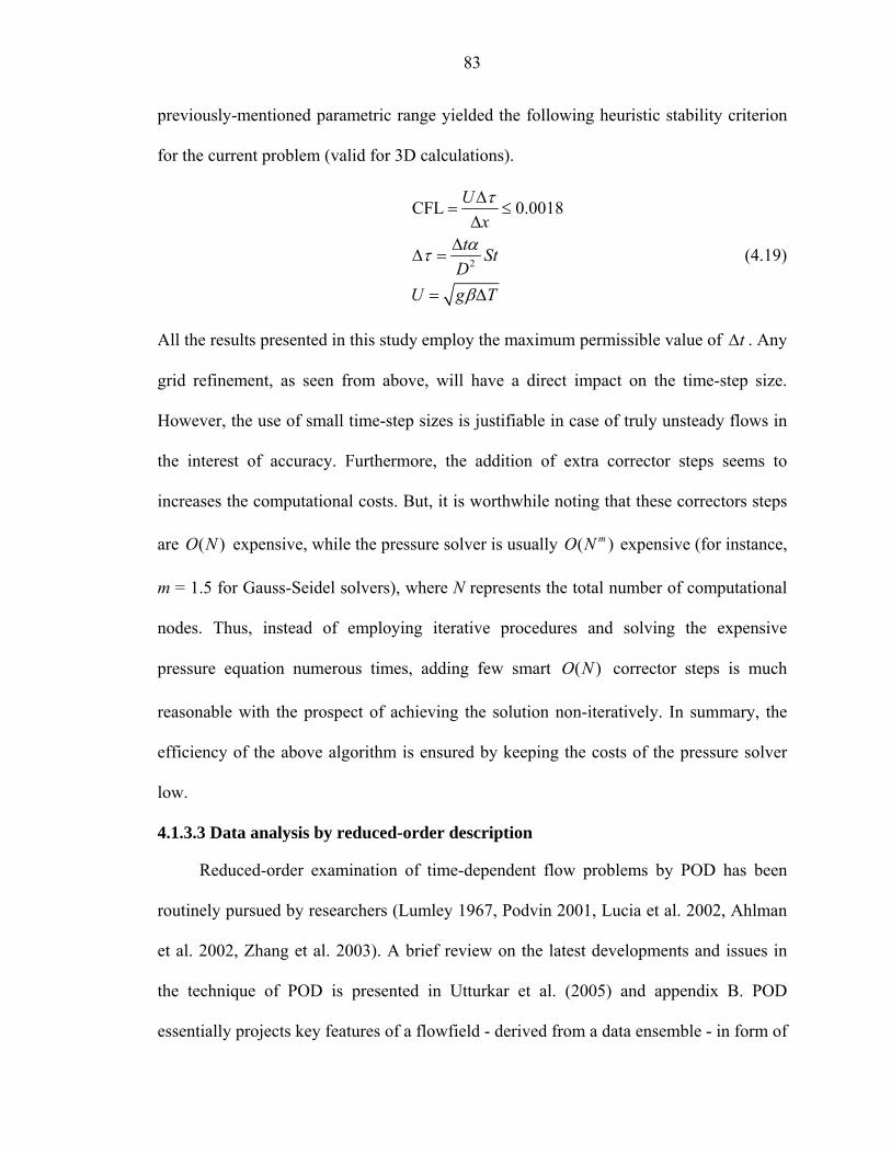
83
previously-mentioned parametric range yielded the following heuristic stability criterion
for the current problem (valid for 3D calculations).
2
CFL 0.0018Ux
t StD
U g T
τ
ατ
β
∆= ≤
∆∆
∆ =
= ∆
(4.19)
All the results presented in this study employ the maximum permissible value of t∆ . Any
grid refinement, as seen from above, will have a direct impact on the time-step size.
However, the use of small time-step sizes is justifiable in case of truly unsteady flows in
the interest of accuracy. Furthermore, the addition of extra corrector steps seems to
increases the computational costs. But, it is worthwhile noting that these correctors steps
are ( )O N expensive, while the pressure solver is usually ( )mO N expensive (for instance,
m = 1.5 for Gauss-Seidel solvers), where N represents the total number of computational
nodes. Thus, instead of employing iterative procedures and solving the expensive
pressure equation numerous times, adding few smart ( )O N corrector steps is much
reasonable with the prospect of achieving the solution non-iteratively. In summary, the
efficiency of the above algorithm is ensured by keeping the costs of the pressure solver
low.
4.1.3.3 Data analysis by reduced-order description
Reduced-order examination of time-dependent flow problems by POD has been
routinely pursued by researchers (Lumley 1967, Podvin 2001, Lucia et al. 2002, Ahlman
et al. 2002, Zhang et al. 2003). A brief review on the latest developments and issues in
the technique of POD is presented in Utturkar et al. (2005) and appendix B. POD
essentially projects key features of a flowfield - derived from a data ensemble - in form of
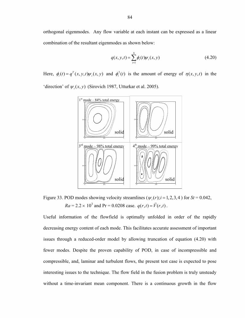
84
orthogonal eigenmodes. Any flow variable at each instant can be expressed as a linear
combination of the resultant eigenmodes as shown below:
1( , , ) ( ) ( , )
N
i ii
q x y t t x yφ ψ=
=∑ (4.20)
Here, ( ) ( , , ) ( , )Ti it q x y t x yφ ψ= and 2 ( )i tφ is the amount of energy of ( , , )x y tη in the
‘direction’ of ( , )i x yψ (Sirovich 1987, Utturkar et al. 2005).
0 0.5 10
0.5
1
0 0.5 10
0.5
1
0 0.5 10
0.5
1
0 0.5 10
0.5
1
Figure 33. POD modes showing velocity streamlines ( ( ); 1, 2,3,4i r iψ = ) for St = 0.042,
Ra = 2.2 × 10³ and Pr = 0.0208 case. ( , ) ( , )q r t V r t=r
.
Useful information of the flowfield is optimally unfolded in order of the rapidly
decreasing energy content of each mode. This facilitates accurate assessment of important
issues through a reduced-order model by allowing truncation of equation (4.20) with
fewer modes. Despite the proven capability of POD, in case of incompressible and
compressible, and, laminar and turbulent flows, the present test case is expected to pose
interesting issues to the technique. The flow field in the fusion problem is truly unsteady
without a time-invariant mean component. There is a continuous growth in the flow
4th mode – 99% total energy 3rd mode – 98% total energy
solid
solid
solid
solid
1st mode – 84% total energy
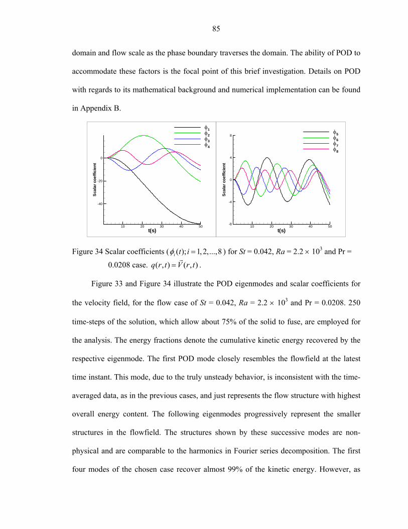
85
domain and flow scale as the phase boundary traverses the domain. The ability of POD to
accommodate these factors is the focal point of this brief investigation. Details on POD
with regards to its mathematical background and numerical implementation can be found
in Appendix B.
t(s)
Sca
larc
oeffi
cien
t
10 20 30 40 50
-40
-20
0
φ1φ2φ3φ4
t(s)S
cala
rcoe
ffici
ent
10 20 30 40 50-8
-4
0
4
8φ5φ6φ7φ8
Figure 34 Scalar coefficients ( ( ); 1, 2,...,8i t iφ = ) for St = 0.042, Ra = 2.2 × 10³ and Pr =
0.0208 case. ( , ) ( , )q r t V r t=r
.
Figure 33 and Figure 34 illustrate the POD eigenmodes and scalar coefficients for
the velocity field, for the flow case of St = 0.042, Ra = 2.2 × 10³ and Pr = 0.0208. 250
time-steps of the solution, which allow about 75% of the solid to fuse, are employed for
the analysis. The energy fractions denote the cumulative kinetic energy recovered by the
respective eigenmode. The first POD mode closely resembles the flowfield at the latest
time instant. This mode, due to the truly unsteady behavior, is inconsistent with the time-
averaged data, as in the previous cases, and just represents the flow structure with highest
overall energy content. The following eigenmodes progressively represent the smaller
structures in the flowfield. The structures shown by these successive modes are non-
physical and are comparable to the harmonics in Fourier series decomposition. The first
four modes of the chosen case recover almost 99% of the kinetic energy. However, as
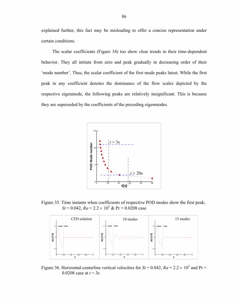
86
explained further, this fact may be misleading to offer a concise representation under
certain conditions.
The scalar coefficients (Figure 34) too show clear trends in their time-dependent
behavior. They all initiate from zero and peak gradually in decreasing order of their
‘mode number’. Thus, the scalar coefficient of the first mode peaks latest. While the first
peak in any coefficient denotes the dominance of the flow scales depicted by the
respective eigenmode, the following peaks are relatively insignificant. This is because
they are superseded by the coefficients of the preceding eigenmodes.
t(s)
PO
DM
ode
num
ber
0 10 20 30 40 500
5
10
15
Figure 35. Time instants when coefficients of respective POD modes show the first peak; St = 0.042, Ra = 2.2 × 10³ & Pr = 0.0208 case
x
v(x,
0.5)
0 0.2 0.4 0.6 0.8 1
-0.1
0
0.1 SolidLiquid
x
v(x,
0.5)
0 0.2 0.4 0.6 0.8 1
-0.1
0
0.1 SolidLiquid
x
v(x,
0.5)
0 0.2 0.4 0.6 0.8 1
-0.1
0
0.1 SolidLiquid
Figure 36. Horizontal-centerline vertical velocities for St = 0.042, Ra = 2.2 × 10³ and Pr = 0.0208 case at t = 3s
CFD solution 10 modes 15 modes
t > 3s
t > 20s
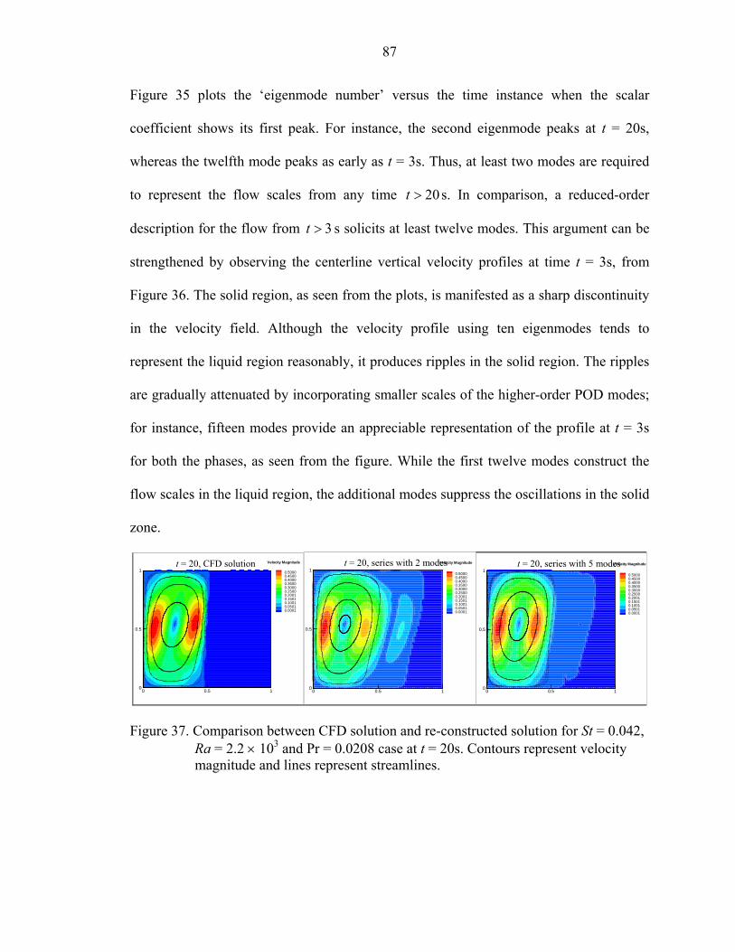
87
Figure 35 plots the ‘eigenmode number’ versus the time instance when the scalar
coefficient shows its first peak. For instance, the second eigenmode peaks at t = 20s,
whereas the twelfth mode peaks as early as t = 3s. Thus, at least two modes are required
to represent the flow scales from any time 20t > s. In comparison, a reduced-order
description for the flow from 3t > s solicits at least twelve modes. This argument can be
strengthened by observing the centerline vertical velocity profiles at time t = 3s, from
Figure 36. The solid region, as seen from the plots, is manifested as a sharp discontinuity
in the velocity field. Although the velocity profile using ten eigenmodes tends to
represent the liquid region reasonably, it produces ripples in the solid region. The ripples
are gradually attenuated by incorporating smaller scales of the higher-order POD modes;
for instance, fifteen modes provide an appreciable representation of the profile at t = 3s
for both the phases, as seen from the figure. While the first twelve modes construct the
flow scales in the liquid region, the additional modes suppress the oscillations in the solid
zone.
0 0.5 10
0.5
1 0.50000.45000.40000.35000.30000.25000.20010.15010.10010.05010.0001
Velocity Magnitude
0 0.5 10
0.5
10.50000.45000.40000.35000.30000.25000.20010.15010.10010.05010.0001
Velocity Magnitude
0 0.5 10
0.5
10.50000.45000.40000.35000.30000.25000.20010.15010.10010.05010.0001
Velocity Magnitude
Figure 37. Comparison between CFD solution and re-constructed solution for St = 0.042, Ra = 2.2 × 10³ and Pr = 0.0208 case at t = 20s. Contours represent velocity magnitude and lines represent streamlines.
t = 20, CFD solution t = 20, series with 2 modes t = 20, series with 5 modes
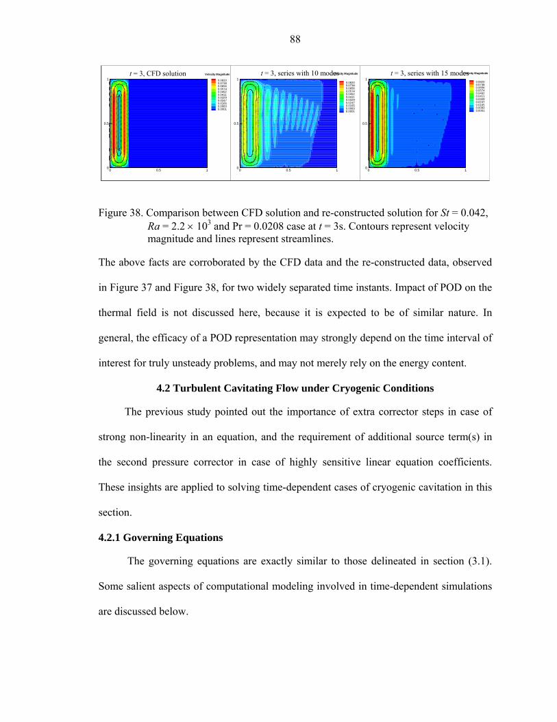
88
0 0.5 10
0.5
1 0.08200.07380.06560.05740.04920.04110.03290.02470.01650.00830.0001
Velocity Magnitude
0 0.5 10
0.5
10.08200.07380.06560.05740.04920.04110.03290.02470.01650.00830.0001
Velocity Magnitude
0 0.5 10
0.5
10.08200.07380.06560.05740.04920.04110.03290.02470.01650.00830.0001
Velocity Magnitude
Figure 38. Comparison between CFD solution and re-constructed solution for St = 0.042, Ra = 2.2 × 10³ and Pr = 0.0208 case at t = 3s. Contours represent velocity magnitude and lines represent streamlines.
The above facts are corroborated by the CFD data and the re-constructed data, observed
in Figure 37 and Figure 38, for two widely separated time instants. Impact of POD on the
thermal field is not discussed here, because it is expected to be of similar nature. In
general, the efficacy of a POD representation may strongly depend on the time interval of
interest for truly unsteady problems, and may not merely rely on the energy content.
4.2 Turbulent Cavitating Flow under Cryogenic Conditions
The previous study pointed out the importance of extra corrector steps in case of
strong non-linearity in an equation, and the requirement of additional source term(s) in
the second pressure corrector in case of highly sensitive linear equation coefficients.
These insights are applied to solving time-dependent cases of cryogenic cavitation in this
section.
4.2.1 Governing Equations
The governing equations are exactly similar to those delineated in section (3.1).
Some salient aspects of computational modeling involved in time-dependent simulations
are discussed below.
t = 3, CFD solution t = 3, series with 10 modes t = 3, series with 15 modes
89
4.2.1.1 Speed of sound modeling
While the speed of sound model in case of steady-state computations is chosen
based on the criterion of fast convergence, for time-dependent computations we employ
the following form (Senocak and Shyy 2002, 2004b; also reviewed in chapter 2).
1 1
1 1
SoS-2 : ( ) ( ) i is
i i
Cp p p pρ ξ
ρ ρρ ρ + −
+ −
−∆ ∂= = =
∆ ∂ − (4.21)
The ability of the above formulation to produce a time-dependent behavior in close
agreement with experimental observations has been previously demonstrated (Senocak
and Shyy 2004b).
4.2.1.2 Turbulence modeling
Similar to the steady-state part, the two-equation based turbulence closure is
adopted for time-dependent computations. In addition to the Launder and Spalding
(1974) approach, we also employ the filter-based modeling (Johansen et al. 2004, Wu et
al. 2004, Wu et al. 2005; also reviewed in chapter 2). The objective is to distill the impact
of the turbulent viscosity field over the unsteady tendencies in the flow. For ease of
reading, the filter-based formulation of eddy viscosity is again mention below.
2
, 0.09mt
C kF Cµ
µ
ρµ
ε= = (4.22)
where, the filter function, F, is expressed in terms of a filter size (∆ ) as:
3/ 2Min[1, ]; 1F C Ckε
∆ ∆
∆= = (4.23)
4.2.1.3 Interfacial velocity model
In the context of either Sharp IDM or Mushy IDM, the interfacial velocity ( ,I nU ) in
time-dependent computations is non-zero, unlike steady-state cases, and needs modeling
90
efforts. Senocak and Shyy (2004b) simply correlated the interfacial velocity ( ,I nU ) to the
vapor normal velocity ( ,v nU ) using the mass conservation formulation at the cavity
interface. In the present study, we seek improvement to the modeling of ,I nU . Consider
the volume integral of the cavitation equation over the entire volume of the cavity, as
shown:
cavity (cavity) cavity
[( ). ] ( )lldV V n da m m dV
tα α + −
∂
∂+ = +
∂∫ ∫ ∫r r
& & (4.24)
The second term on the left-hand-side represents the total flux of the liquid phase fraction
over the cavity interface. In terms of the computational domain and a finite volume
formulation, the above integral can be cast as:
, ,all cells interface area
all cells
( * cell volume) ( )*interfacial area
[( )* cell volume]
ll v n I nU U
tm m
α α
+ −
∂+ − =
∂
+
∑ ∑
∑ & & (4.25)
At this juncture, we defer to an assumption that the unsteadiness of lα is solely due to the
movement of the interface. Thus, if there were no interface movement, we would get:
,interface area all cells
( )*interfacial area [( )* cell volume]l v nU m mα + −= +∑ ∑ & & (4.26)
Subtracting equation (4.26) from (4.25) and discounting the summation, we obtain a
formulation for calculating the interfacial velocity at every node as follows:
,
( * cell volume)
*interfacial area
l
I nl
tU
α
α
∂∂= (4.27)
91
The interfacial area at every cell is computed based on the areas of the cell faces and
local normal direction ( / | |l ln α α= ∇ ∇r rr ). Note that the above formulation yields , 0I nU =
when / 0l tα∂ ∂ = , and is thus consistent with steady-state behavior.
4.2.1.4 Boundary conditions
The boundary conditions for time-dependent cavitating computations are similar to
those in the steady-state part barring the outlet condition. In case of unsteady
calculations, the global mass conservation condition needs to account for the time-
dependent mass accumulation inside the domain. This treatment may render the
computation unstable, especially in context of the PISO algorithm. To circumvent this
numerical difficulty, we impose a ‘mean’ (averaged over outlet plane) value for the
pressure at the outlet plane in our simulations. Thus, the pressure correction is imposed
zero at the outlet boundary. This condition is reasonable given the fact that the tunnels in
the experimental setup (Hord 1973a, 1973b) were mounted between two cryogenic
reservoirs (large Dewars).
4.2.2 Numerical Algorithm
The PISO algorithm is similarly adapted in case of cryogenic cavitation to handle
the large density jumps (due to cavitation), the strong linkage between the temperature
and lα equations, and the temperature-dependence of physical properties. The key steps
of the algorithm in context of cryogenic cavitation are mentioned below. The changes
made in the present context are specifically underscored while the identical steps are
referred to the section (4.1.2).
92
The strongly implicit forms of the continuity, momentum, cavitation, and
temperature equations are as follows (discretized forms of the &k ε equations are
omitted due to their straightforward nature):
11
1 1 1
1 1 1
1 1
1 1
( ) 0
( )
( )
( )
( )
n nn
i i
u n u n n u nP P nb nb u p P
v n v n n v nP P nb nb v p P
n n nP P P nb nb p P P
T n T n T n TP P nb nb P P P
ut
A u A u p H u
A v A v p H v
A G A H S
A T A T H T S
α α α α α
ρ ρ ρ
α α α
++
+ + +
+ + +
+ +
+ +
−+ ∆ =
∆= − ∆ +
= −∆ +
+ = + +
= + +
∑∑
∑∑
(4.28)
Here, PS denotes the explicitly treated source terms in the cavitation and energy
equation, while PGα represents the implicitly treated source term of the cavitation
equation.
(a) Momentum predictor
Logically identical to previous study
(b) First pressure corrector
This step is also similar to previous study except for the convective-diffusive form of the
pressure corrector, as shown below (Cρ is modeled via the speed of sound).
***( ') ( ) ( ')
i i
n nin
i i i i iu uP P
C up u p
t A Aρρ ρ ρ ρ−
+ ∆ ∆ = ∆ + ∆∆
(4.29)
(c) First momentum corrector
Logically identical to previous study
(d) First scalar predictor
93
This step constitutes the prediction of , , , and l T kα ε . Note that the temperature and
cavitation source terms are highly inter-linked. As a result, we resort to adding explicit
corrector steps, as we implemented for the gallium problem. The phase fraction and
temperature is firstly predicted as:
* *
* *
( )
( )
nP P P nb nb p P P
T T T n TP P nb nb p P P
A G A H S
A T A T H T S
α α α α αα α α+ = + +
= + +
∑∑
(4.30)
Following this prediction, we perform the following series of steps 2-5 times.
(i) Update physical properties, namely, , , and l v vpρ ρ based on the predicted
temperature (T*).
(ii) Correct lα explicitly by the pseudo Newton-Raphson technique, as per the
previous study.
(iii) Correct temperature based on the corrected value of lα obtained from (ii)
We note that as many as 5 repetitions are needed for cryogenic cases closer to the critical
point, because of the steep variation of physical properties in that regime. However, 1-2
iterations of the above series may suffice for working conditions (temperature) away
from the critical point.
(e) Update of physical properties
Values of all the physical properties, density, turbulent viscosity ( tµ ), and Cρ are
updated at this point. Since cavitation is characterized by large changes in the density
field, we also update the coefficients and u vP PA A in the momentum equations to account
these changes.
(f) Second pressure corrector
94
*** ** * *'* ** * **
* * *( ") ( [ ] [ ]) ( ")i
i i i
iui ii i i nb nb P iu u u
P P P
C up A u A u A u p
t A A Aρρ ρ ρ ρ−
+ ∆ ∆ = ∆ − − + ∆∆ ∑ ∑ (4.31)
Due to the update on and u vP PA A in the previous step, the derivation of the second
pressure corrector entails the inclusion of an extra term ( ' *** **( )i i iu u uP P PA u A A u= − ) into its
source terms. This term relates to the ‘differential Darcy term’ of the previous study, and
couples the modifications/corrections in the density effects to the pressure field.
(g) Second momentum corrector
Logically identical to previous study
(h) First scalar corrector
Here, all the scalar equations ( , , , and l T kα ε ) undergo explicit corrections, as shown
previously.
(i) Update of physical properties
Identical to step (e)
To enhance the coupling between various flow variables, we repeat all the above
steps ((a) – (i)) one more time.
4.2.3 Results
Time-dependent experimental data in form of pressure signals and/or cavity
snapshots are unavailable for cavitation in cryogenic fluids. As a consequence, we
perform time-dependent computations over the 2D hydrofoil (Hord 1973a) that we
employed for our steady-state cases. The details about the geometry and grid can be
referred from chapter 3. Specifically, cases ‘283B’ and ‘290C’ are selected in conjunction
with the filter-based model to preclude any undesirable dampening effects (filter size,
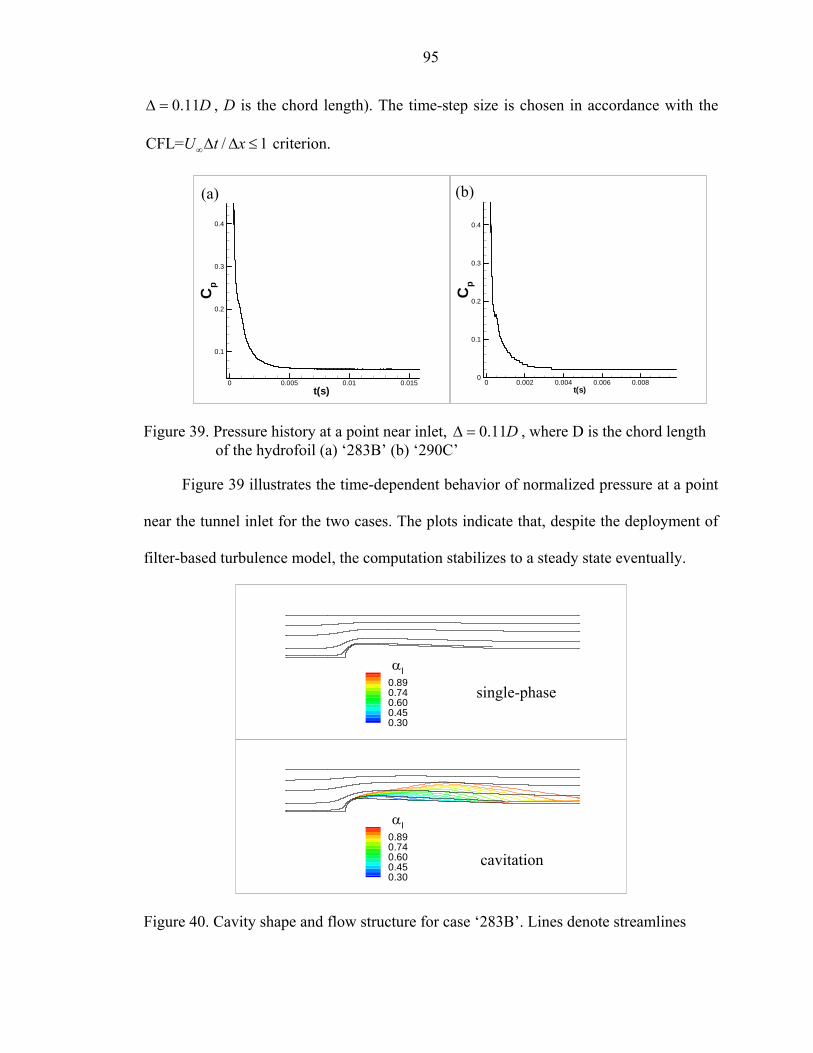
95
0.11D∆ = , D is the chord length). The time-step size is chosen in accordance with the
CFL= / 1U t x∞∆ ∆ ≤ criterion.
t(s)
Cp
0 0.005 0.01 0.015
0.1
0.2
0.3
0.4
t(s)
Cp
0 0.002 0.004 0.006 0.0080
0.1
0.2
0.3
0.4
Figure 39. Pressure history at a point near inlet, 0.11D∆ = , where D is the chord length of the hydrofoil (a) ‘283B’ (b) ‘290C’
Figure 39 illustrates the time-dependent behavior of normalized pressure at a point
near the tunnel inlet for the two cases. The plots indicate that, despite the deployment of
filter-based turbulence model, the computation stabilizes to a steady state eventually.
αl0.890.740.600.450.30
αl0.890.740.600.450.30
Figure 40. Cavity shape and flow structure for case ‘283B’. Lines denote streamlines
(a) (b)
single-phase
cavitation
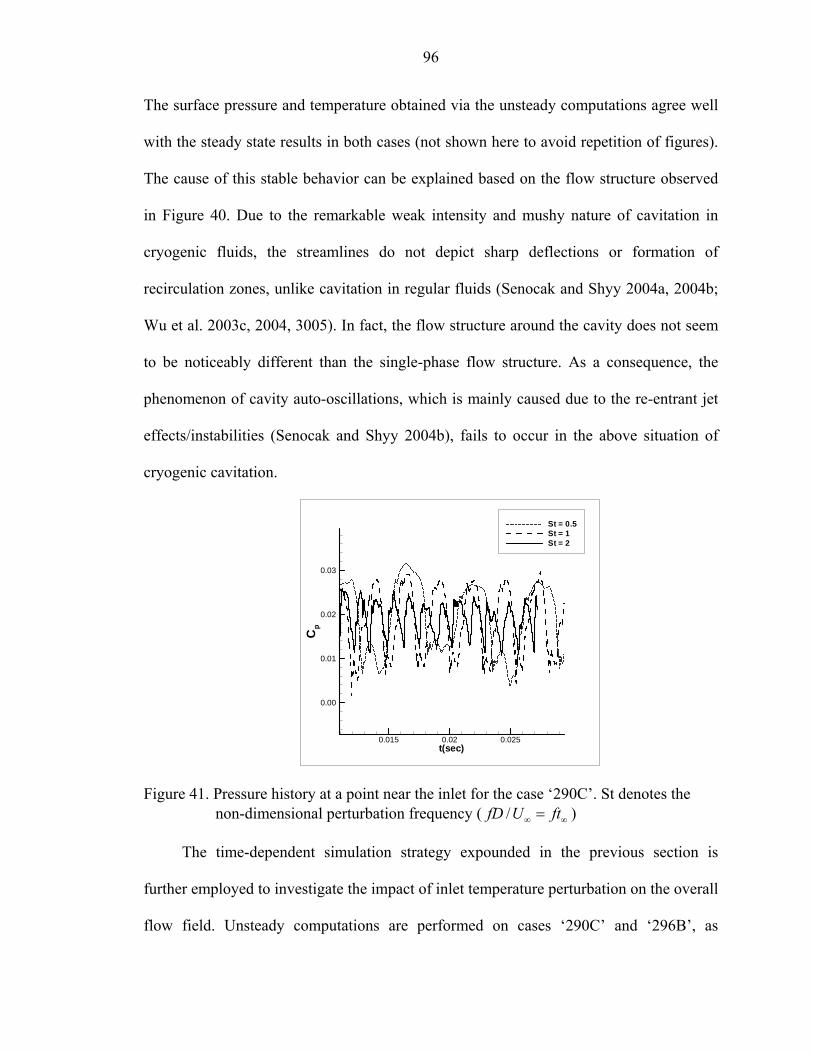
96
The surface pressure and temperature obtained via the unsteady computations agree well
with the steady state results in both cases (not shown here to avoid repetition of figures).
The cause of this stable behavior can be explained based on the flow structure observed
in Figure 40. Due to the remarkable weak intensity and mushy nature of cavitation in
cryogenic fluids, the streamlines do not depict sharp deflections or formation of
recirculation zones, unlike cavitation in regular fluids (Senocak and Shyy 2004a, 2004b;
Wu et al. 2003c, 2004, 3005). In fact, the flow structure around the cavity does not seem
to be noticeably different than the single-phase flow structure. As a consequence, the
phenomenon of cavity auto-oscillations, which is mainly caused due to the re-entrant jet
effects/instabilities (Senocak and Shyy 2004b), fails to occur in the above situation of
cryogenic cavitation.
t(sec)
Cp
0.015 0.02 0.025
0.00
0.01
0.02
0.03
St = 0.5St = 1St = 2
Figure 41. Pressure history at a point near the inlet for the case ‘290C’. St denotes the non-dimensional perturbation frequency ( /fD U ft∞ ∞= )
The time-dependent simulation strategy expounded in the previous section is
further employed to investigate the impact of inlet temperature perturbation on the overall
flow field. Unsteady computations are performed on cases ‘290C’ and ‘296B’, as
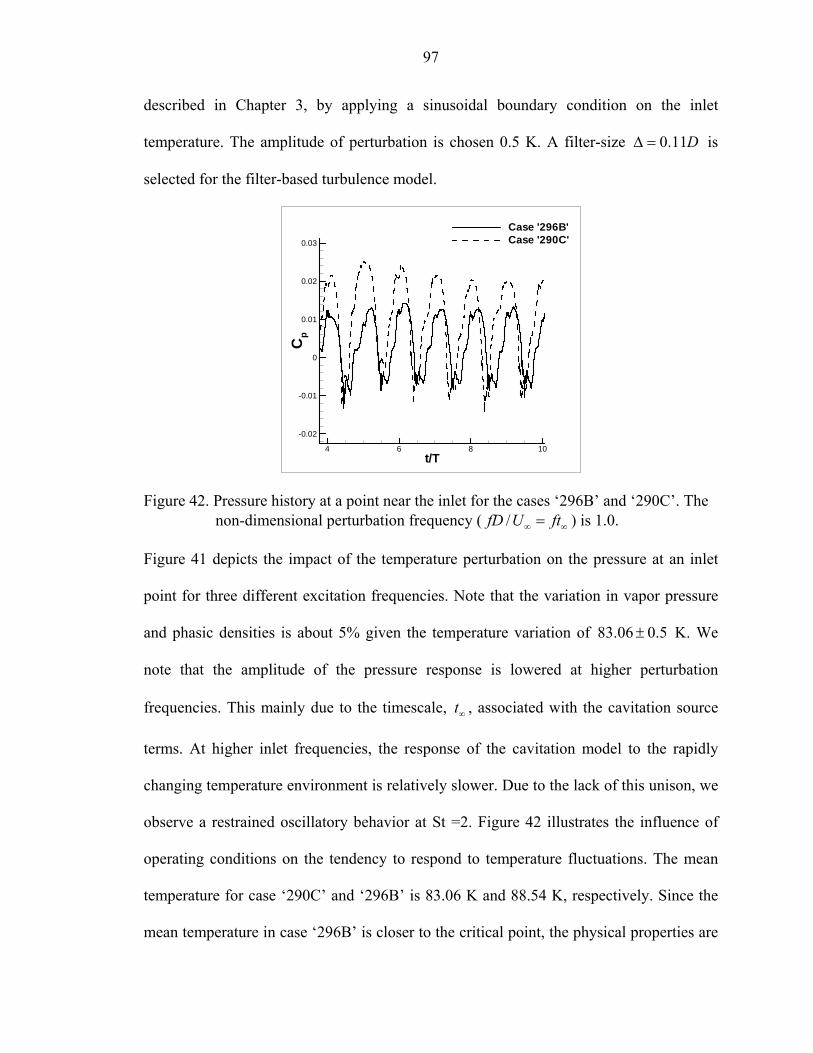
97
described in Chapter 3, by applying a sinusoidal boundary condition on the inlet
temperature. The amplitude of perturbation is chosen 0.5 K. A filter-size 0.11D∆ = is
selected for the filter-based turbulence model.
t/T
Cp
4 6 8 10
-0.02
-0.01
0
0.01
0.02
0.03
Case '296B'Case '290C'
Figure 42. Pressure history at a point near the inlet for the cases ‘296B’ and ‘290C’. The non-dimensional perturbation frequency ( /fD U ft∞ ∞= ) is 1.0.
Figure 41 depicts the impact of the temperature perturbation on the pressure at an inlet
point for three different excitation frequencies. Note that the variation in vapor pressure
and phasic densities is about 5% given the temperature variation of 83.06 0.5± K. We
note that the amplitude of the pressure response is lowered at higher perturbation
frequencies. This mainly due to the timescale, t∞ , associated with the cavitation source
terms. At higher inlet frequencies, the response of the cavitation model to the rapidly
changing temperature environment is relatively slower. Due to the lack of this unison, we
observe a restrained oscillatory behavior at St =2. Figure 42 illustrates the influence of
operating conditions on the tendency to respond to temperature fluctuations. The mean
temperature for case ‘290C’ and ‘296B’ is 83.06 K and 88.54 K, respectively. Since the
mean temperature in case ‘296B’ is closer to the critical point, the physical properties are
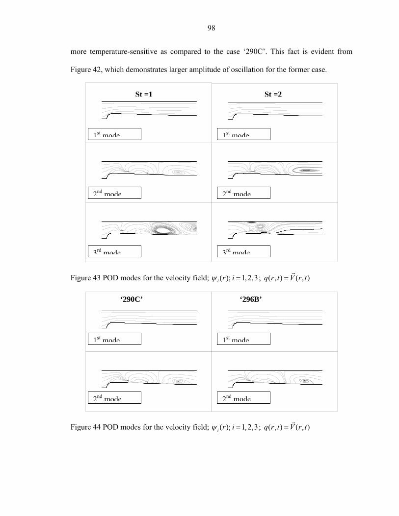
98
more temperature-sensitive as compared to the case ‘290C’. This fact is evident from
Figure 42, which demonstrates larger amplitude of oscillation for the former case.
Figure 43 POD modes for the velocity field; ( ); 1, 2,3i r iψ = ; ( , ) ( , )q r t V r t=r
Figure 44 POD modes for the velocity field; ( ); 1, 2,3i r iψ = ; ( , ) ( , )q r t V r t=r
1st mode 1st mode
2nd mode 2nd mode
3rd mode 3rd mode
St =1 St =2
1st mode 1st mode
2nd mode 2nd mode
‘290C’ ‘296B’
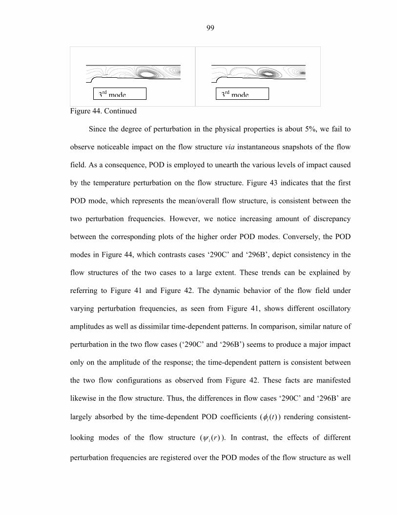
99
Figure 44. Continued
Since the degree of perturbation in the physical properties is about 5%, we fail to
observe noticeable impact on the flow structure via instantaneous snapshots of the flow
field. As a consequence, POD is employed to unearth the various levels of impact caused
by the temperature perturbation on the flow structure. Figure 43 indicates that the first
POD mode, which represents the mean/overall flow structure, is consistent between the
two perturbation frequencies. However, we notice increasing amount of discrepancy
between the corresponding plots of the higher order POD modes. Conversely, the POD
modes in Figure 44, which contrasts cases ‘290C’ and ‘296B’, depict consistency in the
flow structures of the two cases to a large extent. These trends can be explained by
referring to Figure 41 and Figure 42. The dynamic behavior of the flow field under
varying perturbation frequencies, as seen from Figure 41, shows different oscillatory
amplitudes as well as dissimilar time-dependent patterns. In comparison, similar nature of
perturbation in the two flow cases (‘290C’ and ‘296B’) seems to produce a major impact
only on the amplitude of the response; the time-dependent pattern is consistent between
the two flow configurations as observed from Figure 42. These facts are manifested
likewise in the flow structure. Thus, the differences in flow cases ‘290C’ and ‘296B’ are
largely absorbed by the time-dependent POD coefficients ( ( )i tφ ) rendering consistent-
looking modes of the flow structure ( ( )i rψ ). In contrast, the effects of different
perturbation frequencies are registered over the POD modes of the flow structure as well
3rd mode 3rd mode
100
as the POD coefficients. The above observations may tend to vary at higher amplitudes of
the temperature perturbation, a phenomenon which may not be predicted upfront by the
above investigation. Nevertheless, the POD analysis serves to effectively discern the
effects of varying inlet temperature on the flow field by offering a succinct representation
to the time-dependent CFD data.
101
CHAPTER 5 SUMMARY AND FUTURE WORK
5.1. Summary
An effective computational procedure is formulated for simulating turbulent
cavitating flow under cryogenic conditions. The existing framework of equations for
turbulent cavitating flows is coupled with the energy equation to account for the
evaporative cooling effect. The material properties are dynamically updated, as functions
of temperature, to induce the thermo-sensible behavior into the cavitation characteristics.
The derivation of the interfacial dynamics-based cavitation model is revised to
accommodate the mushy features of cavitation typically observed for cryogenic fluids.
The resultant model causes a non-linear decrease and increase in the evaporation and
condensation source term of the original model, respectively.
The cavitation model parameters, which seem to be dependent on the fluid type, in
the newly revised model (referred to as the Mushy IDM) and the Merkle et al. model are
calibrated for liquid Nitrogen and Hydrogen via numerical experimentation. The
sensitivity of predictions to these empirical choices and the uncertainties in material
properties is systematically investigated through a global sensitivity analysis. The results
indicate that the parameters and physical properties, which especially occur in the
cavitation model source terms ( ,, , , , , , , and dest prod v l v mC C t U pβ ρ ρ ρ∞ ∞ ), are more likely
to have a significant impact on the results than others ( , , , and PL K Cµ ). Furthermore, the
pressure and temperature fields pose a trade-off in terms of optimizing their prediction,
102
which is achieved by balancing their agreement with the experimental data. In
comparison with the Merkle et al. Model, the Mushy IDM offers ease in calibration due
to the presence of a single control parameter (β ).
The performance and tendencies of the Mushy IDM depict consistency to the
alternate models in context of the non-cryogenic cases. Subsequently, cryogenic
computations are performed over two geometries (2D hydrofoil and axisymmetric ogive)
with liquid Nitrogen and Hydrogen to extensively assess the framework over wide-
ranging combinations of flow conditions and geometries. The thermodynamic effect is
demonstrated under consistent conditions via the reduction in cavity length and the
increase in effective cavitation number as the working conditions tend towards the critical
point. Reasonable agreement between the computed surface pressure and temperature,
and experimental data is obtained. Specifically, the agreement between the two models is
closer than their respective agreement with the experimental data. In addition, the
predictions of both the models are better; for the pressure field than the temperature field,
and for liquid Nitrogen than liquid Hydrogen. The Hydrogen cases are characterized by
very high inlet velocities, which seemingly have an adverse effect on the predictions. The
deviation of temperature from the experimental values is not consistent between the
hydrofoil and ogive geometry. This inconsistent behavior and the above-mentioned high
velocity conditions for liquid Hydrogen warrant further experimental and numerical
investigation for developing more precise models. Nevertheless, the Mushy IDM, whose
derivation is based on the physical interpretation of cryogenic cavities, is able to offer
reasonable results over all the flow cases.

103
A non-iterative algorithm for pressure-based calculation of multiphase flows is
initiated from the viewpoint of simulating cryogenic cavitation. The Gallium fusion
problem, which is characterized by a non-linear energy equation and strong pressure-
velocity-temperature coupling, is employed as a test case. The algorithm adopts the
framework of the operator splitting strategy (PISO) and incorporates steps to couple the
phase front movement to velocity and pressure fields, and accelerate the convergence of
the non-linear energy equation. Accurate and fairly grid-independent results over a wide-
ranging parameter space are obtained. For inherently unsteady flow problems, the non-
iterative formulation of the algorithm provides substantial computational benefit over the
iterative approach, when accurate and time-dependent information is of interest.
The newly varied PISO algorithm is further adopted for time-dependent
computations of cavitating flow in cryogenic fluids. Impact of perturbing the inlet
temperature on the flow field is investigated via the time-dependent simulations. A stable
performance of the algorithm is observed for all the cases. The weak nature of cavitation
in cryogenic fluids has a modest influence over the flow structure, and thus tends to
reduce the possibility of flow instabilities caused due to re-entrant jet effects. POD is
employed to offer a succinct representation to the time-dependent data. POD is
effectively able to distill dominant flow structures from the voluminous CFD data, and
reveal the impact of the temperature perturbations and flow conditions on the unsteady
behavior of the flow field.
5.2 Future Work
The present study may be extended in the following manner:
(a) Optimization of the cryogenic cavitation models via multi-objective strategies (namely Pareto Front analyses)
104
(b) Systematic experimental probing of the phase transformation rates involved in cavitation to enable development of more precise cavitation models
(c) Critical investigation of various assumptions in the case of liquid Hydrogen to reveal
the cause of the observed discrepancies (d) Investigation of compressibility and turbulence characteristics in cryogenic fluids (e) Deployment/extension of the cryogenic cavitation framework in turbo-machinery
applications
105
APPENDIX A BACKGROUND OF GLOBAL SENSITIVITY ANALYSIS
The surrogate model (response surfaces in our case), g(x), is decomposed as the
sum of functions of increasing dimensionality as:
( ) ( ) ( ) ( )0 12 1 2, , , ,i i ij i j n ni i j
g g g x g x x g x x x<
= + + + +∑ ∑x KL K (A.1)
Equation (A.1) is subjected to the following constraint:
1 1
1
... ...0
0s si i i ig dx =∫ (A.2)
Note that x denotes normalized values of the design variables scaled between 0 and 1,
and 0g represents the mean value ( 0 ( )g g d= ∫ x x ). The constraint in equation (A.2)
renders the decomposition shown in equation (A.1) unique (Sobol 1993). Consequently,
the total variance (V) in the data can be decomposed as:
11 1
( )n
i ij ni i j n
V y V V V= ≤ ≤ ≤
= + + +∑ ∑ KL (A.3)
The partial variances, as shown in equation (A.3), are computed as follows:
( [ | ])( [ | , ])
( [ | , , ])
i i
ij i j i j
ijk i j j ij ik jk i j k
V V E y xV V E y x x V V
V V E y x x x V V V V V V
== − −
= − − − − − −
(A.4)
Here, V and E represent the variance and expected value respectively, and i, j, k, s, and n
are the indices. Thus, the total contribution of a variable ( totaliV ) to the variance in the data
106
can be expressed as the sum of the main effect of the variable and its interactions with
other variables, as shown below.
, , ,main effect
interactions
...totali i ij ijk
j j i j j i k k iV V V V
≠ ≠ ≠
= + + +∑ ∑ ∑14444244443
(A.5)
107
APPENDIX B REVIEW AND IMPLEMENTATION OF POD
B.1 Review
POD was first introduced by Lumley (1967) to investigate coherency of turbulent
flow structures. Since this seminal contribution, POD has been a popular tool to extract
systematically hidden, but deterministic, structures in turbulent flows and can be
extensively found in literature. Gradual progress in this area has established the
application of this technique to laminar flows, as well as to flows under incompressible
and compressible conditions. The latest studies and relevant issues of POD
implementation are reviewed hereafter. Aubry et al. (1988) built a five-mode, reduced-
order model for the wall region of a fully turbulent channel. Their effort was extended by
Podvin (2001), who provided numerical validation of a ten-dimensional model for the
wall layer. The ability of the ten-dimensional model to produce intermittent features,
which are reminiscent of bursting process in a wall layer, was also demonstrated.
Comprehensive POD studies on turbulent mixing layers are available (Delville et al.
1999; Ukeiley et al. 2001), which not only identify the large-scaled structures in the
layer, but also model the dynamic behavior of the lower-order modes. Prabhu et al.
(2001) explored the effect of various flow control mechanisms in a turbulent channel, on
the flow structure in POD modes. The POD modes of various flow control mechanisms
showed significant differences close to the wall but were similar in the channel core.
Similarly, while Liberzon et al. (2001) employed POD to study vorticity characterization
in a turbulent boundary layer, Kostas et al. (2002) adopted the approach to probe PIV
108
data for the backward-facing step flow. Picard and Delville (2000) investigated the effect
of longitudinal pressure distribution on velocity fluctuations in the turbulent shear layer
of a subsonic round jet, using POD. Annaswamy et al. (2002) examined ‘edge-tones’ of
an aircraft nozzle by analyzing the POD modes of azimuthal pressure distribution of a
circular jet. Cizmas and Palacios (2003) gained insight on the turbine rotor-stator
interaction with a lower-order POD investigation. They effectively utilized the time
history and phase-plane plots of the POD coefficients to unravel the key dynamics in the
flow behavior. POD-based investigations on pulsed jet flow field (Bera et al. 2001),
temperature field in flow over heated waves (Gunther and Rohr 2002), and many such
flow cases provide further evidence on the wide applicability of the technique. As
mentioned earlier, POD has been successfully extended to laminar flow cases for
extracting the principle features from time-dependent flow data (Ahlman et al. 2002).
Despite the ongoing progress in POD, several issues of its applicability to variable
density and compressible flows are lately being examined. As indicated before, POD
essentially yields a series, which rapidly converges towards the norm of a variable
( , )q r t . Several past studies intuitively adopted scalar-valued norms for the convergence
criterion. For example, each flow variable namely pressure, density, or any velocity
component was separately decomposed into POD modes. However, Lumley and Poje
(1997) observed that for variable density flows, such as buoyancy-driven flows, an
independent POD analysis may decouple the physical relationship between the flow
variables. They suggested that the norm selection should incorporate the density
variations into the velocity field, to achieve the convergence of a physically relevant
quantity – mass rather than mere velocities - through the POD procedure. However,

109
simultaneous use of two flow variables also poses an important issue of deciding the
significance of each variable in convergence process. Lumley and Poje (1997) suggested
a vector form to ( , )q r t as 1 1 1 2( , ) [ , , , ']q r t C u C v C w C ρ= . In addition, they provided a
mathematical analysis to optimize the values of the weighing factors for expediting the
convergence. Colonius et al. (2002) extended the above argument by examining the
impact of the norm selection on POD analysis of compressible flow over a cavity. POD
modes independently obtained by scalar-valued norms of pressure and velocity were
compared to those derived by vector-based norms. The choice of the vector,
2( , ) [ , , , ]1
q r t u v w cγ
=−
, was chosen with ingenuity so as to yield a norm as shown
below:
12 2 2 2 3 22|| ( , ) || [ ( ) ]
1q r t u v w c dr
γΩ
= + + +−∫ (B.1)
The above norm effectively yielded a linear series that converged towards the stagnation
enthalpy instead of mere kinetic energy. Colonius et al. (2002) further reported that
scalar-valued POD modes were unable to capture key processes such as acoustic
radiation, which heavily rely on coupling mechanisms between the variables. In
comparison, the vector-valued POD modes were in cohort with the compressible flow
dynamics. Ukeiley et al. (2002) employed 0
( , ) [ , , , , ]T Tu v wq r tU U U T T
ρρ
∞
∞ ∞ ∞ ∞ ∞
−=
− to perform
POD on numerical data of compressible mixing layer. The variables, as shown above,
were normalized by their freestream values to ensure a rational weighing of their
fluctuations. A slow convergence towards the multi-variable norm was reported. POD
implementation was also shown to face serious issues in case of supersonic flows due to
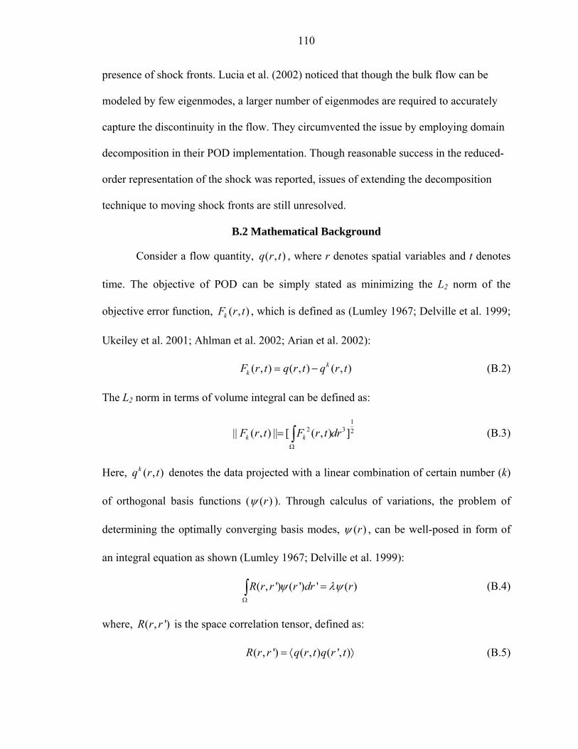
110
presence of shock fronts. Lucia et al. (2002) noticed that though the bulk flow can be
modeled by few eigenmodes, a larger number of eigenmodes are required to accurately
capture the discontinuity in the flow. They circumvented the issue by employing domain
decomposition in their POD implementation. Though reasonable success in the reduced-
order representation of the shock was reported, issues of extending the decomposition
technique to moving shock fronts are still unresolved.
B.2 Mathematical Background
Consider a flow quantity, ( , )q r t , where r denotes spatial variables and t denotes
time. The objective of POD can be simply stated as minimizing the L2 norm of the
objective error function, ( , )kF r t , which is defined as (Lumley 1967; Delville et al. 1999;
Ukeiley et al. 2001; Ahlman et al. 2002; Arian et al. 2002):
( , ) ( , ) ( , )kkF r t q r t q r t= − (B.2)
The L2 norm in terms of volume integral can be defined as:
12 3 2|| ( , ) || [ ( , ) ]k kF r t F r t dr
Ω
= ∫ (B.3)
Here, ( , )kq r t denotes the data projected with a linear combination of certain number (k)
of orthogonal basis functions ( ( )rψ ). Through calculus of variations, the problem of
determining the optimally converging basis modes, ( )rψ , can be well-posed in form of
an integral equation as shown (Lumley 1967; Delville et al. 1999):
( , ') ( ') ' ( )R r r r dr rψ λψΩ
=∫ (B.4)
where, ( , ')R r r is the space correlation tensor, defined as:
( , ') ( , ) ( ', )R r r q r t q r t= ⟨ ⟩ (B.5)

111
In the context of classical application of POD to turbulent structures, the angular brackets
denote ensemble average of statistically stationary turbulent flow data. However, the
angular brackets in context of the present study interchangeably represent time-averaging
of either unsteady RANS or laminar solutions. This approach is often referred in
literature as the ‘snapshot POD approach’ (Sirovich 1987; Zhang et al. 2003), where
every instantaneous solution is considered as a ‘snapshot’ of the data. Solution of
equation (B.4), which is also subjected to a constraint of unitary norm || ( ) || 1rψ = , yields
the orthogonal eigenmodes ( )n rψ with corresponding eigenvalues nλ . Consequently,
solution of the flow quantity at each time step can be exactly expressed as a linear
combination of the eigenmodes (also known as POD modes) in the following form.
1( , ) ( ) ( )
N
n nn
q r t t rφ ψ=
=∑ (B.6)
The time-dependent multipliers or scalar coefficients, ( )n tφ , are obtained by projecting
the solution at each time step on the basis functions as shown.
3( ) ( , ) ( )n nt q r t r d rφ ψΩ
= ∫ (B.7)
Merely, from a standpoint of equation (B.6), infinite choices for the basis functions
( )n rψ are available. But, the basis functions determined in conjunction with the minima
of || ( , ) ||kF r t ensure optimal and sequential extraction of key features from the data
ensemble, enabling truncation of the series (B.6) with fewer POD modes. Thus, succinct
expression of a voluminous data ensemble, with focus on its salient aspects is facilitated
through the lower-order modes.
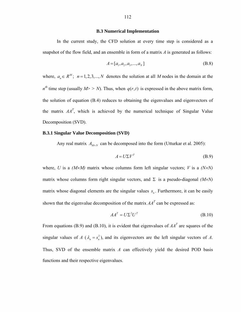
112
B.3 Numerical Implementation
In the current study, the CFD solution at every time step is considered as a
snapshot of the flow field, and an ensemble in form of a matrix A is generated as follows:
1 2 3[ , , ,..., ]NA a a a a= (B.8)
where, ; 1, 2,3,...,Mna R n N∈ = denotes the solution at all M nodes in the domain at the
nth time step (usually M> > N). Thus, when ( , )q r t is expressed in the above matrix form,
the solution of equation (B.4) reduces to obtaining the eigenvalues and eigenvectors of
the matrix AAT, which is achieved by the numerical technique of Singular Value
Decomposition (SVD).
B.3.1 Singular Value Decomposition (SVD)
Any real matrix M NA × can be decomposed into the form (Utturkar et al. 2005):
TA U V= Σ (B.9)
where, U is a (M×M) matrix whose columns form left singular vectors; V is a (N×N)
matrix whose columns form right singular vectors, and Σ is a pseudo-diagonal (M×N)
matrix whose diagonal elements are the singular values ns . Furthermore, it can be easily
shown that the eigenvalue decomposition of the matrix AAT can be expressed as:
2T TAA U U= Σ (B.10)
From equations (B.9) and (B.10), it is evident that eigenvalues of AAT are squares of the
singular values of A ( 2n nsλ = ), and its eigenvectors are the left singular vectors of A.
Thus, SVD of the ensemble matrix A can effectively yield the desired POD basis
functions and their respective eigenvalues.
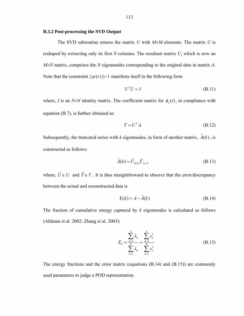
113
B.3.2 Post-processing the SVD Output
The SVD subroutine returns the matrix U with M×M elements. The matrix U is
reshaped by extracting only its first N columns. The resultant matrix U, which is now an
M×N matrix, comprises the N eigenmodes corresponding to the original data in matrix A.
Note that the constraint || ( ) || 1rψ = manifests itself in the following form
TU U I= (B.11)
where, I is an N×N identity matrix. The coefficient matrix for ( )n tφ , in compliance with
equation (B.7), is further obtained as:
TU AΓ = (B.12)
Subsequently, the truncated series with k eigenmodes, in form of another matrix, ˆ( )A k , is
constructed as follows:
ˆ ˆ ˆ( ) M k k NA k U × ×= Γ (B.13)
where, U U∈ and Γ∈Γ . It is thus straightforward to observe that the error/discrepancy
between the actual and reconstructed data is
ˆ( ) ( )k A A kΕ = − (B.14)
The fraction of cumulative energy captured by k eigenmodes is calculated as follows
(Ahlman et al. 2002; Zhang et al. 2003):
2
1 1
2
1 1
k k
n nn n
k N N
n nn n
sE
s
λ
λ
= =
= =
= =∑ ∑
∑ ∑ (B.15)
The energy fractions and the error matrix (equations (B.14) and (B.15)) are commonly
used parameters to judge a POD representation.
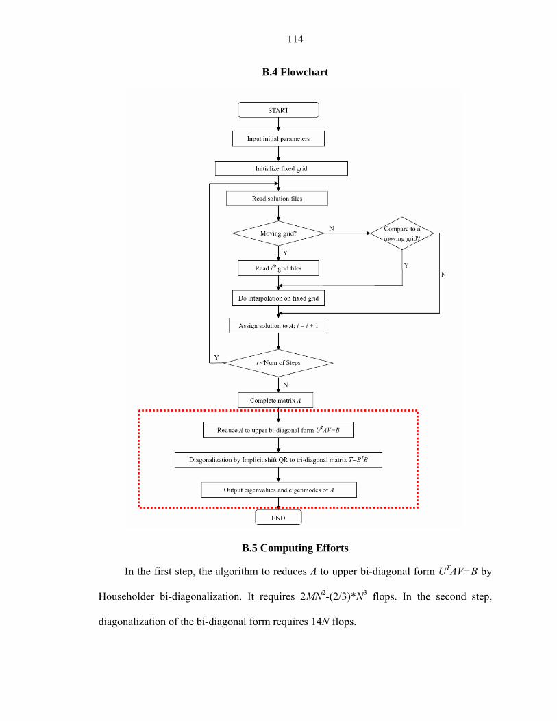
114
B.4 Flowchart
B.5 Computing Efforts
In the first step, the algorithm to reduces A to upper bi-diagonal form UTAV=B by
Householder bi-diagonalization. It requires 2MN2-(2/3)*N3 flops. In the second step,
diagonalization of the bi-diagonal form requires 14N flops.

115
The SVD subroutine (shown in dotted rectangle) is adopted from Press et al. (1992)
which is essentially a Fortran-90 code. Creating subroutines to read the CFD data into
matrix A, determine the coefficient matrix, reconstruct the truncated series, perform
various error estimates and output the solution, constitutes a major part of the present
effort. The Fast Fourier Transform (FFT) and least square analyses are performed on
MATLAB and MATHCAD.
116
LIST OF REFERENCES
Ahlman, D., Soderlund, F., Jackson, J., Kurdilla, A. and Shyy, W., 2002, “Proper Orthogonal Decomposition for Time-dependent Lid-driven Cavity Flows,” Numerical Heat Transfer, Part B, vol. 42, pp. 285-306.
Ahuja, V., Hosangadi, A. and Arunajatesan, S., 2001, “Simulations of Cavitating Flows Using Hybrid Unstructured Meshes,” Journal of Fluids Engineering, vol. 123, pp. 331-340.
Annaswamy, A., Choi, J.J., Sahoo, D., Alvi, F.S. and Lou, H., 2002, “Active Closed Loop Control of Supersonic Impinging jet Flows Using POD models,” Proc. 41st IEEE Conference on Decision and Control, pp. 3294-3299, Las Vegas, NV.
Arian, E., Fahl, M. and Sachs, E.W., 2002, “Managing POD Models by Optimization Methods,” Proc. 41st IEEE Conference on Decision and Control, pp. 3300-3305, Las Vegas, NV.
Athavale, M.M., Li, H.Y., Jiang, Y. and Singhal, A.K., 2000, “Application of Full Cavitation Model to Pumps and Inducers,” Presented at 8th International Symposium on Transport Phenomenon and Dynamics, Honolulu, HI.
Athavale, M.M. and Singhal, A.K., 2001, “Numerical Analysis of Cavitating Flows in Rocket Turbopump Elements,” AIAA Paper 2001-3400.
Aubry, N., Holmes, P., Lumley, J.L. and Stone, E., 1988, “The Dynamics of Coherent Structures in the Wall Region of the Wall Boundary Layer,” J. Fluid Mech., vol. 192, no. 15, pp. 115-173.
Batchelor, G.K., 1967, An Introduction to Fluid Dynamics, Cambridge University Press, New York.
Bera, J.C., Michard, M., Grosjean, N. and Comte-Bellot, G., 2001, “Flow Analysis of Two-Dimensional Pulsed Jets by Particle Image Velocimetry,” Experiments in Fluids, vol. 31, pp. 519-532.
Brennen, C.E., 1994, Hydrodynamics of Pumps, Oxford University Press, New York
Brennen, C.E., 1995, Cavitation and Bubble Dynamics, Oxford University Press, New York.
117
Chavanne, X., Balibar, S. and Caupin, F., 2002, “Heterogeneous Cavitation in liquid Helium-4 near a Glass Plate,” Journal of Low Temperature Physics, vol. 126, no. 1, pp. 615-620.
Chen, Y. and Heister, S.D., 1996, “Modeling Hydrodynamic Non-equilibrium in Cavitation Flows,” Journal of Fluids Engineering, vol. 118, pp. 172-178.
Chuan, C.H., Schreiber, W.C., Kuo, C.H. and Ganesh, S., 1991, “The Effect of Convection on the Interface Location between Solid and Liquid Aluminum,” Proc. ASME HTD, vol. 163, pp. 79-84.
Cizmas, P.G.A. and Palacios, A., 2003, “Proper Orthogonal Decomposition of Turbine Rotor-Stator Interaction”, J. Propulsion and Power, vol. 19, no. 2, pp. 268-281.
Clarke, J.W.L. and Leighton, T.G., 2000, “A Method for Estimating Time-dependent Acoustic cross-sections of Bubbles and Bubble clouds prior to the Steady State,” J. Acoust. Soc. Am., vol. 107, no. 4, pp. 1922-1929.
Colonius, T., Rowley, C.W., Freund, J.B. and Murray, R., 2002, “On the Choice of Norm for Modeling Compressible Flow Dynamics at Reduced-order Using the POD,” Proc. 41st IEEE Conference on Decision and Control, pp. 3273-3278, Las Vegas, NV.
Coutier-Delgosha, O. and Astolfi, J.A., 2003, “Numerical Prediction of the Cavitating Flow on a Two-Dimensional Symmetrical Hydrofoil With a Single Fluid Model,” Presented at Fifth International Symposium on Cavitation, Osaka, Japan.
Daney, D.E., 1988, “Cavitation in flowing Superfluid Helium,” Cryogenics, vol. 28, pp. 132-136.
Delannoy, Y. and Kueny, J.L., 1990, “Cavity Flow Predictions Based on the Euler Equations,” ASME Cavitation and Multiphase Flow Forum, Toronto, Canada.
Delannoy, Y. and Reboud, J.L., 1993, “Heat and Mass Transfer on a Vapor Cavity,” Proc. ASME Fluids Engineering Conference, Washington, DC, vol. 165, pp. 209-214.
Delville, J., Ukeiley, L., Cordier, L., Bonnet, J.P. and Glauser, M., 1999, “Examination of Large-scale Structures in a Turbulent Plane Mixing Layer: Part 1 - Proper Orthogonal Decomposition,” J. Fluid Mech., vol. 391, pp. 91-122.
Deshpande, M., Feng, J. and Merkle, C.L., 1994, “Cavity Flow Predictions Based on the Euler Equations,” Journal of Fluids Engineering, vol. 116, pp. 36-44.
Deshpande, M., Feng, J. and Merkle, C.L., 1997, “Numerical Modeling of the Thermodynamic Effects of Cavitation,” Journal of Fluids Engineering, vol. 119, pp. 420-427.
118
Edwards, J.R., Franklin, R.K. and Liou, M.S., 2000, “Low-Diffusion Flux Splitting Methods for Real Fluid Flows with Phase Transitions,” AIAA Journal, vol. 38, no. 9, pp. 1624-1633.
Franc, J.P., Avellan, F., Belahadji, B., Billard, J.Y., Briancon, L., Marjollet, Frechou, D., Fruman, D. H., Karimi, A., Kueny, J.L., and Michel, J. M., 1995, La Cavitation: Mecanismes Physiques et Aspects Industriels, Presses Universitaires de Grenoble, Grenoble (EDP Sciences), pp. 28, 141, 142, 144, 449, France.
Franc, J.P., Janson, E., Morel, P., Rebattet, C. and Riondet, M., 2001, “Visualizations of Leading Edge Cavitation in an Inducer at Different Temperatures,” Presented at Fourth International Symposium on Cavitation, Pasadena, Canada.
Franc, J.P., Rebattet, C. and Coulon, A., 2003, “An Experimental Investigation of Thermal Effects in a Cavitating Inducer,” Presented at Fifth International Symposium on Cavitation, Osaka, Japan.
Fruman, D.H., Benmansour, I. and Sery, R., 1991, “Estimation of the Thermal Effects on Cavitation of Cryogenic Liquids,” Proc. Cavitation and Multiphase Forum, pp. 93-96.
Fruman, D.H., Reboud, J.L. and Stutz, B., 1999, “Estimation of Thermal Effects in Cavitation of Thermosensible Liquids,” Int. J. Heat and Mass Transfer, vol. 42, pp. 3195-3204.
Gau, C. and Viskanta, R., 1986, “Melting and Solidification of a Pure Metal on a Vertical Wall,” J. Heat Transfer, vol. 108, pp. 174-181.
Gopalan, S. and Katz, J., 2000, “Flow Structure and Modeling Issues in the Closure Region of Attached Cavitation,” Phys. Fluids, vol. 12, no. 4, pp. 895-911.
Gunther, A. and Rohr, P.R., 2002, “Structure of Temperature Field in a Flow over Heated Waves,” Experiments in Fluids, vol. 33, pp. 920-930.
Hord, J., 1973a, “Cavitation in Liquid Cryogens, II – Hydrofoil,” NASA Contractor Report, NASA CR – 2156.
Hord, J., 1973b, “Cavitation in Liquid Cryogens, III – Ogives,” NASA Contractor Report, NASA CR – 2242.
Hosangadi, A., Ahuja, V. and Ungewitter, R.J., 2002, “Simulations of Cavitating Inducer Flowfields,” JANNAF 38th Combustion Subcommittee Meeting, Sandestin, FL.
Hosangadi, A. and Ahuja, V., 2003, “A Generalized Multi-phase Framework for Modeling Cavitation in Cryogenic Fluids,” AIAA Paper 2003-4000.
Hosangadi, A., Ahuja, V. and Ungewitter, R.J., 2003, “Generalized Numerical Framework for Cavitation in Inducers,” ASME Paper FEDSM2003-45408.

119
Hosangadi, A. and Ahuja, V., 2005, “Numerical Study of Cavitation in Cryogenic Fluids,” J. Fluids Engineering, vol. 127, pp. 267-281.
Iga, Y., Nohmi, M., Goto, A., Shin, B.R. and Ikohagi, T., 2003, “Numerical Study of Sheet Breakoff Phenomenon on a Cascade Hydrofoil,” Journal of Fluids Engineering, vol. 125, pp. 643-651.
Issa, R.I., 1985, “Solution of the Implicitly Discretized Fluid Flow Equations by Operator Splitting,” J. Comp. Phys., vol. 62, pp. 40-65.
JMP®, 2002, The Statistical Discovery SoftwareTM, version 5.0, SAS Institute Inc., Cary, NC, U.S.A.
Johansen, S., Wu, J. and Shyy, W., 2004, “Filter-based Unsteady RANS Computations,” Int. J. Heat and Fluid Flow, vol. 25, pp. 10-21.
Kakegawa, A. and Kawamura, T., 2003, “An Experimental Study on Oxidation of Organic Compounds by Cavitating Water-Jet,” Presented at Fifth International Symposium on Cavitation, Osaka, Japan.
Kalamuck, K.M., Chahine, G.L., Hsiao, C.T. and Choi, J.K., 2003, “Remediation and Disinfection of Water Using Jet Generated Cavitation,” Presented at Fifth International Symposium on Cavitation, Osaka, Japan.
Kawanami, Y., Kato, H., Tanimura, M. and Tagaya, Y., 1997, “Mechanism and Control of Cloud Cavitation,” Journal of Fluids Engineering, vol. 119, pp. 788-794.
Khodadadi, J.M. and Zhang, Y., 2001, “Effects of Buoyancy-driven convection on melting with Spherical Containers,” Int. J. Heat and Mass Transfer, vol. 44, pp. 1605-1618.
Kim, S., Lee, B. and Cho, S., 2000, “A Front Layer Predictor-Corrector Algorithm with pseudo Newton-Raphson Method for the Phase Change Heat Conduction Problems,” Int. Comm. Heat Mass Transfer, vol. 27, no. 7, pp. 1003 – 1012.
Kirschner, I.N., 2001, “Results of Selected Experiments Involving Supercavitating Flow,” VKI Lecture Series on Supercavitating Flow, VKI Press, Brussels, Belgium.
Knapp, R.T., Daily, J.W. and Hammitt, F.G., 1970, Cavitation, McGraw-Hill, New York.
Kostas, J., Soria, J. and Chong, M.S., 2002, “Particle Image Velocimetry Measurements of a Backward-facing Step Flow,” Experiments in Fluids, vol. 33, pp. 838-853.
Kunz, R.F., Boger, D.A., Stinebring, D.R., Chyczewski, T.S., Lindau, J.W. and Gibeling, H.J., 2000, “A Preconditioned Navier-Stokes Method for Two-phase Flows with Application to Cavitation,” Comput. Fluids, vol. 29, pp. 849-875.
120
Kunz, R.F., Lindau, J.W., Kaday, T.A. and Peltier, L.J., 2003, “Unsteady RANS and Detached Eddy Simulations of Cavitating Flow over a Hydrofoil,” Presented at Fifth International Symposium on Cavitation, Osaka, Japan.
Lacroix, M., 1989, “Computation of Heat Transfer During Melting of a Pure Substance from an Isothermal Wall,” Num. Heat Transfer, Part B, vol. 15, pp. 191-210.
Lacroix, M. and Voller, V.R., 1990, “Finite Difference Solutions of Solidification Phase Change Problems: Transformed Versus Fixed Grids,” Num. Heat Transfer, Part B, vol. 17, pp. 25-41.
Lambare, H., Roche, P., Balibar, S., Maris, H.J., Andreeva, O.A., Guthmann, C., Keshishev, K.O. and Rolley, E., 1998, “Cavitation in superfluid Helium-4 at Low Temperature,” Eur. Phys. Jou., B 2, pp. 381-391.
Larrarte, F., Pauchet, A., Bousquet, P.H. and Fruman, D.H., 1995, “On Morphology of Natural and Ventilated Cavities,” Proc. Cavitation and Multiphase Flow, vol. 210, pp. 31-38.
Launder, B.E. and Spalding, D.B., 1974, “The Numerical Computation of Turbulent Flows,” Comp. Meth. Appl. Mech. Eng., vol. 3, pp. 269-289.
Lecoffre, Y., 1999, Cavitation Bubble Trackers, A.A. Balkema, Brookfield, VT.
Leighton, T.G., Wilkinson, M., Walton, A.J. and Field, J.E., 1990, “Studies of non-linear Bubble Oscillations in a Simulated Acoustic Field,” Eur. J. Phys., vol. 11, pp. 352-358.
Lemmon, E.W., McLinden, M.O., and Huber, M.L., 2002, REFPROP: Reference Fluid Thermodynamic and Transport Properties, NIST Standard Database 23, version 7.0.
Lertnuwat, B., Sugiyama, K. and Matsumoto, Y., 2001, “Modeling of Thermal Behavior inside a Bubble,” Presented at Fourth International Symposium on Cavitation, Pasadena, Canada.
Liberzon, A., Gurka, R. and Hetsroni, G., 2001, “Vorticity Characterization in a Turbulent Boundary Layer using PIV and POD Analysis,” 4th International Symposium on Particle Image Velocimetry, Gottingen, Germany, Paper 1184.
Lindau, J.W., Kunz, R.F., Boger, D.A., Stinebring, D.R. and Gibeling, H.J., 2002, “High Reynolds Number Unsteady, Multiphase CFD Modeling of Cavitating Flows,” Journal of Fluids Engineering, vol. 124, pp. 607-616.
Lucia, D.J., King, P.I. and Beran, P.S., 2002, “Domain Decomposition for Reduced-order Modeling of a Flow with Moving Shocks,” AIAA Journal, Tech. Notes, vol. 40, no. 11, pp. 2360-2362.
121
Lumley, J.L., 1967, “The Structure of Inhomogeneous Turbulent Flows,” Atmospheric Turbulence and Radio Wave Propagation, pp. 166-178.
Lumley, J.L. and Poje, A., 1997, “Low Dimensional Models for Flows with Variable Density,” Phys. Fluids, vol. 9, no. 7, pp. 2023-2031.
Merkle, C.L., Feng, J. and Buelow, P.E.O., 1998, “Computational Modeling of Dynamics of Sheet Cavitation,” Proc. 3rd International Symposium on Cavitation, Grenoble, France.
Muzio, G., Alippi, A., Bettucci, A., Farrelly, F. and Germano, M., 1998, “A Numerical method for studying non-linear Bubble Oscillations in Acoustic Cavitation,” Ultrasonics, vol. 36, pp. 553-557.
Myers, R.H. and Montgomery, D.C., 1995, Response Surface Methodology, John Wiley and Sons, Inc., New York.
National Aeronautics and Space Administration (NASA) Online Facts, 1991, http://www-pao.ksc.nasa.gov/kscpao/nasafact/count2.htm (last access: July 12, 2005)
Ohl, C.D., Arora, M., Ikink, R., Delius, M. and Wolfrum, B., 2003, “Drug Delivery Following Shock Wave Induced Cavitation,” Presented at Fifth International Symposium on Cavitation, Osaka, Japan.
Oliveira, P.J. and Issa, R.I., 2001, “Improved PISO Algorithm for the Computation of Buoyancy-driven Flows,” Numerical Heat Transfer, Part B, vol. 40, pp. 473-493.
Owen, A., 1992, “Orthogonal Arrays for: Computer Experiments, Integration and Visualization,” Statistica Sinica, vol. 2, no. 2, pp. 439-452.
Picard, C. and Delville, J., 2000, “Pressure Velocity Coupling in A Subsonic Round Jet,” Int. J. of Heat and Fluid Flow, vol. 21, pp. 359-364.
Podvin, B., 2001, “On the Adequacy of the Ten-dimensional Model for the Wall Layer,” Phys. Fluids, vol. 13, no. 1, pp. 210-224.
Prabhu, R.D., Collis, S.S. and Chang, Y., 2001, “The Influence of Control on Proper Orthogonal Decomposition of Wall-bounded Turbulent Flow,” Phys. Fluids, vol. 13, no. 2, pp. 520-537.
Press, W.H., Teukolsky, S.A., Vetterling, W.T. and Flannery, B.P., 1992, Numerical Recipes in Fortran – The Art in Scientific Computing, Cambridge University Press, New York.
122
Preston, A., Colonius, T. and Brennen, C.E., 2001, “Towards Efficient Computation of Heat and Mass Transfer Effects in the Continuum Model for Bubbly Cavitating Flows,” Presented at Fourth International Symposium on Cavitation, Pasadena, California.
Qin, Q., Song, C.C.S. and Arndt, R.E.A., 2003, “A Virtual Single-Phase Natural Cavitation Model and its Application to Cav2003 Hydrofoil,” Presented at Fifth International Symposium on Cavitation, Osaka, Japan.
Rachid, F.B.F., 2003, “A Thermodynamically consistent Model for Cavitating Flows of Compressible Fluids,” Int. J. Non-linear Mechanics, vol. 38, pp. 1007-1018.
Rapposelli, E. and Agostino, L.D., 2003, “A Barotropic Cavitation Model with Thermodynamic Effects,” Presented at Fifth International Symposium on Cavitation, Osaka, Japan.
Reboud, J.L., Sauvage-Boutar, E. and Desclaux, J., 1990, “Partial Cavitation Model for Cryogenic Fluids,” Cavitation and Multiphase Flow Forum, Toronto, Canada.
Rouse, H. and McNown, J.S., 1948, “Cavitation and Pressure Distribution, Head Forms at Zero Angle of Yaw,” Studies in Engineering, vol. 32, State University of Iowa, Aemes, Iowa.
Ruggeri, R.S. and Moore, R.D., 1969, “Method of Prediction of Pump Cavitation Performance for Various Liquids, Liquid Temperatures and Rotation Speeds,” NASA Technical Note, NASA TN D-5292.
Sarosdy, L.R. and Acosta, A.J., 1961, “Note on Observations of Cavitation in Different Fluids,” Paper 60-WA-83, ASME Winter Annual Meeting, New York.
Sato, H., Sun, X.W., Odagawa, M., Maeno, K. and Honma, H., 1996, “An Investigation on the Behavior of Laser Induced Bubble in Cryogenic Liquid Nitrogen,” Journal of Fluids Engineering, vol. 118, pp. 850-856.
Saurel, R., Cocchi, J.P. and Butler, P.B., 1999, “Numerical Study of Cavitation in the wake of a Hypervelocity under water Projectile,” J. Propulsion and Power, vol. 15, no. 4, pp. 513-522.
Senocak, I. and Shyy, W., 2002, “A Pressure-based Method for Turbulent Cavitating Flow Computations,” J. Comp. Phys., vol. 176, pp. 363-383.
Senocak, I. and Shyy, W., 2003, “Computations of Unsteady Cavitation with a Pressure-based Method,” ASME Paper FEDSM2003-45009.
Senocak, I. and Shyy, W., 2004a, “Interfacial Dynamics-Based Modeling of Turbulent Cavitating Flows, Part-1: Model Development and Steady-State Computations,” Int. J. for Num. Methods in Fluids, vol. 44, pp. 975-995.

123
Senocak, I. and Shyy, W., 2004b, “Interfacial Dynamics-Based Modeling of Turbulent Cavitating Flows, Part-2: Time-Dependant Computations,” Int. J. for Num. Methods in Fluids, vol. 44, pp. 997-1016.
Shen, Y. and Dimotakis, P., 1989, “The Influence of Surface Cavitation on Hydrodynamic Forces,” Proc. 22nd ATTC, St. Johns, pp. 44-53.
Shyy, W., Rao, M.M. and Udaykumar, H.S., 1995, “Scaling Procedure and Finite Volume Computations of Phase-change problems with Convection,” Engg. Analysis with Boundary Elements, vol. 16, pp. 123-147.
Shyy, W. and Thakur, S.S., 1994, “A Controlled Variation Scheme in a Sequential Solver for Recirculating Flows. Part I. Theory and Formulation,” Numerical Heat Transfer B-Fund, vol. 25, no. 3, pp. 245-272.
Shyy, W., Thakur, S.S., Ouyang, H., Liu, J. and Blosch, E., 1997, Computational Techniques for Complex Transport Phenomenon, Cambridge University Press, NewYork.
Shyy, W., Udaykumar, H.S., Rao, M.M. and Smith, R., 1998, Computational Fluids Dynamics with Moving Boundaries, Taylor and Francis Press, Philadelphia, PA.
Singhal, A.K., Vaidya, N. and Leonard, A.D., 1997, “Multi-dimensional Simulation of Cavitating Flows Using a PDF Model for Phase Change,” ASME Paper FEDSM97-3272.
Singhal, A.K., Athavale, M.M., Li, H. and Jiang, Y., 2002, “Mathematical Basis and Validation of the Full Cavitation Model,” Journal of Fluids Engineering, vol. 124, pp. 617-624.
Sirovich, L., 1987, “Turbulence and the Dynamics of Coherent Structures: Part I-III,” Quart. Appl. Math., vol. 45, pp. 561-590.
Sobol, I.M., 1993, “Sensitivity Analysis for Nonlinear Mathematical Models,” Mathematical Modeling & Computational Experiment, vol. 1, no. 4, pp. 407-414.
Soyama, H. and Macodiyo, D., 2003, “Improvement of Fatigue Strength on Stainless Steel by Cavitating Jet in Air,” Presented at Fifth International Symposium on Cavitation, Osaka, Japan.
Tanguay, M. and Colonius, T., 2003, “Progress in Modeling and Simulation of Shock Wave Lithotripsy (SWL),” Presented at Fifth International Symposium on Cavitation, Osaka, Japan.
Thakur, S. and Wright, J., 2004, “A Multiblock Operator-Splitting Algorithm for Unsteady Flows at All Speeds in Complex Geometries,” Int. J. Num. Meth. Fluids, vol. 46, pp. 383-413.
124
Thakur, S.S., Wright, J. and Shyy, W., 2002, “STREAM: A Computational Fluid Dynamics and Heat Transfer Navier-Stokes Solver,” Streamline Numerics Inc. and Computational Thermo-Fluids Laboratory, Department of Mechanical and Aerospace Engineering Technical Report, University of Florida, Gainesville, FL.
Tokumasu, T., Kamijo, K. and Matsumoto, Y., 2002, “A Numerical Study of Thermodynamic Effects of Sheet Cavitation,” Proceedings of ASME FEDSM’02, Montreal, Quebec, Canada.
Tokumasu, T., Sekino, Y. and Kamijo, K., 2003, “A new Modeling of Sheet Cavitation Considering the Thermodynamic Effects,” Presented at Fifth International Symposium on Cavitation, Osaka, Japan.
Ukeiley, L., Cordier, L., Manceau, R., Delville, J., Glauser, M. and Bonnet, J.P., 2001, “Examination of Large-scale Structures in a Turbulent Plane Mixing Layer: Part 2 - Dynamical Systems Model,” J. Fluid Mech., vol. 441, pp. 67-108.
Ukeiley, L., Kannepalli, C. and Arunajatesan, S., 2002, “Development of Low dimensional Models for Control of Compressible Flows,” Proc. 41st IEEE Conference on Decision and Control, pp. 3282-3287, Las Vegas, NV.
Utturkar, Y., Zhang, B., and Shyy, W., 2005, “Reduced-order Description of Fluid Flow with Moving Boundaries by Proper Orthogonal Decomposition,” Int. J. Heat and Fluid Flow, vol. 26, pp. 276-288.
Venkateswaran, S., Lindau, J.W., Kunz, R.F. and Merkle, C., 2002, “Computation of Multiphase Mixture Flows with Compressiblity Effects,” J. Comp. Phys., vol. 180, pp. 54-77.
Ventikos, Y. and Tzabiras, G., 2000, “A Numerical methods for Simulation of Steady and Unsteady Cavitating Flows,” Comput. Fluids, vol. 29, pp. 63-88.
Versteeg, H.K. and Malalasekera, W., 1995, An Introduction to Computational Fluid Dynamics: The Finite Volume Method, Pearson Education Limited, England.
Wang, G., 1999, “A Study on Safety assessment of a Hollow Jet Valve accompanied by Cavitation,” Ph.D. Dissertation, Tohuku University, Sendai, Japan.
Wang, G., Senocak, I., Shyy, W., Ikohagi, T. and Cao, S., 2001, “Dynamics of Attached Turbulent Cavitating Flows,” Prog. Aero. Sci., vol. 37, pp. 551-581.
Weisend, J.G., 1998, Handbook of Cryogenic Engineering, Taylor and Francis, Philadelphia, PA.
Wu, J., Senocak, I., Wang, G., Wu, Y. and Shyy, W., 2003a, “Three-Dimensional Simulation of Turbulent Cavitating Flows in a Hollow-Jet Valve,” Journal of Comp. Modeling in Eng. & Sci., vol. 4, no. 6, pp. 679-690.
125
Wu, J., Utturkar, Y., Senocak, I., Shyy, W. and Arakere, N., 2003b, “Impact of Turbulence and Compressibility Modeling on Three-Dimensional Cavitating Flow Computations,” AIAA Paper 2003-4264.
Wu, J., Utturkar, Y. and Shyy, W., 2003c, “Assessment of Modeling Strategies for Cavitating Flow around a Hydrofoil,” Presented at Fifth International Symposium on Cavitation, Osaka, Japan.
Wu, J., Shyy, W., and Johansen, S., 2004, “Filter-based Unsteady RANS Computations for Single-Phase and Cavitating Flows,” ASME Paper HT-FED2004-56181.
Wu, J., Wang, G., and Shyy, W., 2005, “Time-dependent Turbulent Cavitating Flow Computations with Interfacial Transport and Filter-based Models, accepted for publication, Int. J. Num. Meth. Fluids.
Zhang, B., Lian, Y. and Shyy, W., 2003, “Proper Orthogonal Decomposition for Three-dimensional Membrane Wing Aerodynamics,” AIAA Paper 2003-3917.
126
BIOGRAPHICAL SKETCH
Yogen Utturkar was born in Mumbai (formerly Bombay), India, on June 12, 1977.
He obtained his B.E. (Bachelor of Engineering) degree in mechanical engineering from
the University of Mumbai in May 1999. He worked as a software engineer from 1999-
2000 before proceeding to pursue graduate studies in the United States. Yogen obtained
his master’s degree in mechanical engineering (minor in engineering sciences) at the
University of Florida in April 2002. He investigated synthetic jet flow fields for his M.S.
thesis under the tutelage of Dr. Rajat Mittal.
Yogen worked towards his doctoral dissertation under the guidance of Dr. Wei
Shyy (chair) and Dr. Nagaraj Arakere (cochair). His research interests comprised
numerical modeling of thermodynamic effects in cryogenic cavitation, reduced-order
description of simulated data by Proper Orthogonal Decomposition (POD), and
development of efficient algorithms for problems involving phase change.
Yogen met his wife, Neeti Pathare, during his graduate years. They married in May
2002 and completed their Ph.D. degree from the same institution (University of Florida).