thermodynamic modeling and mechanical properties …
TRANSCRIPT

The Pennsylvania State University
The Graduate School
THERMODYNAMIC MODELING AND MECHANICAL PROPERTIES MODELING
OF LONG PERIODIC STACKING ORDERED (LPSO) PHASES
A Dissertation in
Materials Science and Engineering
by
Hongyeun Kim
© 2019 Hongyeun Kim
Submitted in Partial Fulfillment
of the Requirements
for the Degree of
Doctor of Philosophy
August 2019

ii
The dissertation of Hongyeun Kim was reviewed and approved* by the following:
Zi-Kui Liu
Distinguished Professor of Materials Science and Engineering
Dissertation Advisor
Chair of Committee
Ismaila Dabo
Assistant Professor of Materials Science and Engineering
Hojong Kim
Assistant Professor of Materials Science and Engineering
Adri van Duin
Professor of Department of Mechanical & Nuclear Engineering
Laszlo Kecskes
Special Member,
Adjunct Associate Research Scholar, Johns Hopkins University
Suzanne Mohney
Professor of Materials Science and Engineering
Administrative
*Signatures are on file in the Graduate School

iii
ABSTRACT
Recently, there has been an increasing interest in long periodic stacking ordered (LPSO)
phases in Mg alloys due to their lightweight, high elastic and mechanical properties. The Vickers
indentation hardness and Young’s modulus of LPSO phases have reached 470% and 140%,
respectively, of that of pure Mg. Although theoretical and experimental studies have revealed the
phase constitutions and crystal structures of LPSO phases including the formation of the noble
solute atom clusters, which is also known as L12-type clusters, their phase stabilities and the origin
of their enhanced mechanical properties are not yet solved. To further improve the properties and
design the alloys, a thorough understanding of the phase equilibria and the origin of the mechanical
properties of LPSO phases are therefore needed.
In this dissertation, the elastic properties of LPSO phases in the Mg-Al-Gd system were
studied using first-principles calculations. Since LPSO phases have been reported to enhance the
strength and ductility of Mg alloys due to their high elastic properties, the effects of atomic
arrangements in terms of Gd-Al L12-type clusters on LPSOs’ elastic properties in the Mg-Al-Gd
system were studied using first-principles calculations. Four types of LPSO phases (10H, 18R,
14H, and 24R) were investigated with and without an interstitial atom in the center of the L12-type
clusters. Furthermore, the calculated Poisson’s ratios of each LPSO phases from this study is also
used as an important parameter for obtaining thermodynamic properties.
Thermodynamic modelling of the four LPSO phases, i.e., 10H, 18R, 14H, and 24R, in the
Mg-Al-Gd system was performed using the CALPHAD (calculation of phase diagram) approach
with input from the present first-principles calculations and experimental data in the literature.
Sublattice models were developed to describe these LPSO phases. Especially, an L12-type clusters
in the FCC stacking layers of LPSO phases and the atomic occupancy in the center of L12 cluster
were considered based on experimental observations and energetics from first-principles

iv
calculations. The calculated phase equilibrium results are in good agreement with experiments
about the phase stability of 14H and 18R and the mole fraction of Gd and Al in these LPSO phases.
The present modeling provides a new approach to describe the thermodynamic properties of LPSO
phases that can be applied to other alloy systems.
Material hardness is a good indicator of mechanical properties. However, since there is no
hardness model that can be used for LPSO phases, a large portion of the effort in this dissertation
is devoted to developing a suite of hardness models, which can be divided into three categories:
hardness model for both brittle and ductile materials, temperature-dependent hardness model and
hardness model for layered structures. In turn, the hardness of the LPSO phases is
obtained/modeled, based on these hardness models that were developed.
Hardness, defined as the resistance of a material to deformation, is a quick and efficient
measure of mechanical performance of materials. However, to date no comprehensive predictive
models exist for both metals and ceramics. We present a physics-based model that is capable of
predicting Vickers indentation hardness of both brittle and ductile materials with model inputs from
either first-principles calculations or experiments. Particularly, we go beyond the elastic properties
of materials commonly used in the literature and introduce the plastic properties of materials in
terms of active slip systems, including the Peierls-Nabarro flow stress, Burgers vector and slip
plane spacing into the model. It is demonstrated that this model can predict hardness values from
below 0.1 GPa of pure aluminum to above 100 GPa of diamond. The predictive power of the new
model has the potential to significantly advance the computational discovery and design of new
materials with enhanced performance.
Furthermore, a new temperature dependent hardness model is also proposed based on the
thermally activated dislocation width in combination with our previous Vickers hardness model.
The thermally activated dislocation width, a basic building block for the temperature dependent
Peierls-Nabarro flow stress in the hardness model, captures dislocation-diffusion mechanisms

v
during the materials’ deformation. In the proposed model, the material hardness is determined by
(a) diffusion mechanisms, (b) slip systems, (c) diffusing species, and (d) phase transformations.
The model has been calibrated for and agrees well with experimental hot hardness results of 16
materials, which were available from the public domain, including metals and ceramics.
The hardness model for layered structures is also modeled in order to investigate the origin
of the Hall-Petch relation in structures with twinned, tilt and twist boundaries, especially, hardness
enhancement of these structures based on material’s active slip systems of the structure as well as
the elastic properties since the slip systems are crucial to understanding the deformation of
materials. The active slip systems in this model are modulated by the relaxation of atomic positions
near the boundaries. This proposed model explains the flow stress and the hardness changes as the
twin or grain size in the structure changes, that is previously considered as an outcome of the Hall-
Petch relation.

vi
TABLE OF CONTENTS
List of Figures .......................................................................................................................... viii
List of Tables ........................................................................................................................... xiii
Acknowledgements .................................................................................................................. xiv
Chapter 1 Introduction ............................................................................................................. 1
1.1 Motivation .................................................................................................................. 1 1.2 Overview .................................................................................................................... 2
Chapter 2 Elastic Properties of Long Periodic Stacking Ordered Phases in Mg-Al-Gd
Alloys: A First-Principles Study ...................................................................................... 4
2.1 Introduction ................................................................................................................. 4 2.2 Computational Methods .............................................................................................. 6 2.3 Results and Discussion ............................................................................................... 8
2.3.1 Structural Analysis of the LPSO Phases ......................................................... 8 2.3.2 Elastic Properties of the LPSO Phases ............................................................ 12 2.3.3 Electronic Properties of the LPSOs ................................................................. 21
Chapter 3 First-Principles Calculations and Thermodynamic Modelling of Long Periodic
Stacking Ordered (LPSO) Phases in Mg-Al-Gd .............................................................. 25
3.1 Introduction ................................................................................................................ 25 3.2 First-Principles Calculations ...................................................................................... 26 3.3 CALPHAD Modeling of Phase Equilibria ................................................................. 30 3.4 Results and Discussion ............................................................................................... 34
Chapter 4 Predictive Modeling of Hardness of Brittle and Ductile Materials ......................... 46
4.1 Introduction ................................................................................................................ 46 4.2 Presentation of the New Model .................................................................................. 48 4.3 Validation and Prediction ........................................................................................... 49 4.4 Discussion .................................................................................................................. 56 4.5 Full Derivation of the Hardness Model ...................................................................... 60
4.5.1 Derivation of the Hardness Equation .............................................................. 60 4.5.2 Evaluation of Model Parameters ..................................................................... 63 4.5.2.1 hT/hp Ratio ................................................................................................. 63 4.5.2.2 Parameter c ................................................................................................... 70
Chapter 5 Temperature Dependent Hardness Model: the Study of Thermally Activated
Dislocation Width ............................................................................................................ 85
5.1 Introduction ................................................................................................................ 85

vii
5.2 Results and Discussion ............................................................................................... 87 5.2.1 Change of Diffusion Mechanism .................................................................... 88 5.2.2 Change of the Active Slip System ................................................................... 91 5.2.3 Phase Transformation at Finite Temperature .................................................. 92 5.2.4 Change of the Diffusion Species ..................................................................... 95 5.2.5 Phase Transformations During Indentation ..................................................... 98
5.3 Modeling Procedure ................................................................................................... 98 5.3.1 Derivation ........................................................................................................ 98 5.3.2 Temperature-Dependent Elastic Properties ..................................................... 105
Chapter 6 Hardness Modeling for Layered Structures: The Origin of Hall-Petch Relation .... 110
6.1 Introduction ................................................................................................................ 110 6.2 Methodology .............................................................................................................. 113
6.2.1 Derivation of Peierls-Nabarro Flow Stress for Twinned Structures ............... 113 6.2.2 First-Principles Calculations ........................................................................... 119
6.3 Results and Discussion ............................................................................................... 119
Chapter 7 Hardness Modeling of LPSO Phases....................................................................... 127
7.1 Methodology .............................................................................................................. 127 7.2 Results and Discussion ............................................................................................... 128
Chapter 8 Conclusions and Future Work ................................................................................. 131
8.1 Conclusions ................................................................................................................ 131 8.2 Future Work ............................................................................................................... 133
Appendix A Complete Elastic Stiffness Matrixes of 10H, 18R and 24R LPSO Phases .......... 134
Appendix B Thermo-Calc Mg-Al-Gd Database ...................................................................... 136
Bibliography ............................................................................................................................ 166

viii
LIST OF FIGURES
Figure 2.1 The LPSO structures of 10H (a), 18R (b), 14H (c), and 24R (d) together with
the in-plane L12 cluster ordering (e) and the Gd8Al6 L12 cluster with an interstitial
(int.) atom Gd, Mg or Al (f). Blue box stands for the unit cell of each LPSO
structures and the red bracket with SB stands for structural block for each LPSO
structure. 𝑑𝑖𝑛𝑡𝑟𝑎𝑐𝑙𝑢𝑠𝑡𝑒𝑟 and 𝑑𝑖𝑛𝑡𝑒𝑟𝑐𝑙𝑠𝑡𝑒𝑟 stands for the 2NN RE-RE intracluster
and intercluster distances, 𝑤clusterand ℎcluster stands for the L12 cluster width and
height. ............................................................................................................................... 10
Figure 2.2 Calculated bulk moduli of the LPSO phases with respect to number of layers
in structural block; (a) bulk modulus from EOS fitting and (b) bulk modulus from
VRH approach. Red dash lines indicate the bulk and shear moduli of HCP Mg. ........... 15
Figure 2.3 (a) comparison of bulk moduli both from VRH and EOS fitting as a function
of formation energies of LPSOs, and (b) Young’s modulus along [0001] direction
trend as a function of volumetric formation energies (𝐸𝑓/𝑉) of LPSOs. ........................ 17
Figure 2.4 Changes in (a) C11, (b) C33, (c) C44 and (d) C66 elastic constants as a function
of the number of layers in structural blocks. .................................................................... 18
Figure 2.5 Comparison between C11 and the energy contribution of interstitial atom in
L12 cluster. ....................................................................................................................... 19
Figure 2.6 Relationship of L12 cluster width with (a) C11, and (b) C66 elastic constants. ........ 20
Figure 2.7 Crystallographic orientation dependence of the Young’s and Shear modulus of
10H, 18R, 14H and 24R LPSO phase at 0K, between [0001] and <1120> 𝜃 is the
angle from <1120>. The orientation dependencies of the Young’s modulus and
shear modulus of HCP Mg are shown for comparison. ................................................... 21
Figure 2.8 Differential charge density plots of the LPSOs with or without interstitial
atoms. Differential charge density plots of (a) 10H, (b) 18R, (c) 14H, and (d) 24R
LPSO. The reference states used in this study are (e) 2H and (f) 14H LPSO with Mg
only; (g), (h), and (i) are the 14H LPSO with Al-int., Gd-int., and Mg-int. Red
arrows indicate the charge density connections between the {0001] planes.
Isosurfaces are 0.0021 (e/Å 3) and the Mg atom sizes are exaggerated for better
visualization. .................................................................................................................... 23
Figure 3.1 Experimentally observed LPSO phase compositions of 14H (a) and 18R (b)
LPSO phases[8], [19], [23], [65], [91]–[101]. Dash lines refer to the composition
ranges of this model. ........................................................................................................ 31
Figure 3.2. (a) Phonon dispersion curves of HCP Mg with experimental data[105] (red
circles), and b) phonon DOS curves of HCP Mg and Mg LPSO phases of 10H, 18R,
14H, and 24R. .................................................................................................................. 35

ix
Figure 3.3 Comparison of (a) heat capacity of HCP Mg with experimental data from
SGTE[82], (b) heat capacities of Mg-only LPSO phases, and (c) Gibbs energy
differences of various pure Mg LPSO phases with respect to HCP Mg. ......................... 37
Figure 3.4 Formation energies of endmembers of the 10H, 18R, 14H, and 24R LPSO
phases at 0 K. The data sets of GdIIAlIIIMgIV-Saal (×) were taken from the
literature[14]. .................................................................................................................... 39
Figure 3.5 (a) Composition ranges of GdIIAlIII(Mg, Gd, Al, and Va)IV endmembers of the
10H(o), 18R(⟡), 14H(x), and 24R(∇) LPSOs, (b) formation energies (in kJ/mole-
atom) of the GdIIAlIII(Mg(x), Gd(∇), Al(⟡), and Va(o))IV endmembers at 0 K in
compositional space. ........................................................................................................ 40
Figure 3.6 Isothermal sections of the Mg-Al-Gd system at 673 K (a) and 798 K (b). All
experiment data (the thick lines and the symbols) at 673 K were measured by De
Negri et al.[110] (∇ : Al3Mg2 + FCC Al + Lav C36, ∆: GdMg + GdMg3, □: MgGd,
⟡: GdMg + AlGd2, ⧖:GdMg + Lav C15 + GdMg3), those at 798.15K were taken
from Kishida et al.[6], [109], including HCP Mg + Al2Gd (Laves C15) + 18R LPSO
(○[109]) and HCP Mg + Mg5Gd + 18R LPSO (∇[6] and ⟡[6]) phases. ........................ 41
Figure 3.7 Mg-corner of the isothermal sections of the Mg-Al-Gd system at (a) 838.15 K,
(b) 823.15 K, (c) 798.15 K, (d) 773.15 K, (e) 723.15 K, and (f) 673.15 K, with
experimental compositions from Lu et al.[111] at 838.15 K (∇) with HCP Mg +
Al2Gd (Laves C15) + 18R LPSO phases in equilibrium, at 823.15 K from Dai et
al.[112] (*) with 18R LPSO phase composition of Mg–7.9 at.% Al–10.9 at.%
(Gd+Y), at 798.15 K from Kishida et al. with HCP Mg + Al2Gd (Lav C15) + 18R
LPSO (○[109]) and HCP Mg + Mg5Gd + 18R LPSO (∇[6] and ⟡[6]) phases in
equilibrium, and at 773.15 K from Gu et al.[113] with 18R LPSO, respectively. The
small triangles represent the composition ranges of GdIIAlIII(Mg, Gd and Al)IV
endmembers. .................................................................................................................... 43
Figure 3.8 An enlarged view of the isothermal section of the Mg-Al-Gd system at 798.15
K, showing the composition homogeneity range of the 18R LPSO phase. Blue
triangle indicates the composition ranges of GdIIAlIII(Mg, Gd, Al, and Va)IV
endmembers as the same triangle as Figure 3.5. .............................................................. 44
Figure 3.9 Isopleth sections of the Mg-Al-Gd phase diagram with the molar ratio of
Al:Gd being 0.7 (a) and an enlarged view of the Mg-rich region (b), with
experimental compositions from Lu et al.[111] at 838.15 K (+) with HCP Mg, Lav
C15 and LPSO (18R) phases in equilibrium, and from Kishida et al.[17] at 673.15K
(*) with HCP Mg, Mg5Gd and LPSO (14H + 18R) phases, respectively. ....................... 45
Figure 4.1 Schematics of (a) Vickers tip geometry, (b) geometry changes during
indentation, and (c) a side view of indentation. ............................................................... 48
Figure 4.2 Hardness comparisons of (a) FCC, (b) BCC, and (c) HCP materials with
respect to experimental data. Solid and open symbols represent the predicted values
using elastic properties from experiments and first-principles calculations. Red
x
dashed lines indicate value equality, vertical dotted lines connect the hardness
between the slip systems. ................................................................................................. 53
Figure 4.3 Hardness comparisons of ceramic materials with respect to experimental data.
Solid and open symbols represent the predicted values using elastic properties from
experiments and first-principles calculations. Red dashed lines indicate value
equality, vertical dotted lines show the differences between glide edge and shuffle
screw slip systems. ........................................................................................................... 56
Figure 4.4 Hardness comparisons of all tested materials with respect to experimental data.
Solid and open symbols represent the predicted values using elastic properties from
experiments and first-principles calculations. The experiments for all materials both
hardness and elastic properties data from Table 4.6. Red dashed lines indicate value
equality. ............................................................................................................................ 57
Figure 4.5 Comparison of Peierls-Nabarro flow stress at 0 K with experimental yield
stress at low temperatures (4~77K) as a function of dislocation width. Data and
references are listed in Table 4.3. ..................................................................................... 58
Figure 4.6 Indentation ductility index as a function of dislocation width at room
temperature....................................................................................................................... 60
Figure 4.7 (a) Stress(𝜏)-strain(𝛾) curve during shear deformation. (b) typical Load(F)-
displacement(h) curve during indentation process. .......................................................... 62
Figure 4.8 Typical Load-displacement curves (a) F-h curve and (b) 𝐹-h curve. Red lines
are loading curves and blue lines are unloading curves, and green dot line represents
only the plastic contribution from Equation 4.16. ............................................................ 65
Figure 4.9 Peierls-Nabarro flow stress (𝜏𝑃𝑁) and ideal shear stress (𝜏𝑇) at 4.7 K and 7 K
in terms of dislocation width (𝑤0) from Refs.[206]–[209] shown in Table 4.3 and
Table 4.5........................................................................................................................... 68
Figure 4.10 Comparison of ℎ𝑇/ℎ𝑝 ratio between experiment from Table 4.4 and the
present model. .................................................................................................................. 70
Figure 4.11 Exponential relationship of the scaling factor c (from Equation 4.31) for FCC
metals with data from Table 4.4. ...................................................................................... 72
Figure 4.12 Plots of parameter c from experimental data (Equation 4.31) with data from
Table 4.4 (a) with respect to 𝑏/𝑠2 and (b) with respect to the model (Equation 4.36). ... 73
Figure 4.13 Comparison of experimental and calculated (VRH averaged) shear moduli
with elastic stiffness constant data from Shang et al.[42]. ............................................... 83
Figure 4.14 Comparison of experimental and calculated (VRH averaged) bulk moduli
with elastic stiffness constant data from Shang et al.[42]. ............................................... 84

xi
Figure 5.1 Activation energy for self-diffusion modeling. All the data and references are
in Table 5.3. ..................................................................................................................... 88
Figure 5.2 Predicted temperature dependent hardness of FCC metals. All the
experimental data is from Lozinskii[313]. ....................................................................... 90
Figure 5.3 Predicted temperature dependent hardness of FCC Rh (a) and Ir (b), and BCC
Mo (c) and W (d) metals. All the experimental data is from Lozinskii[313](■) and
Stephens et al.[316](▲). .................................................................................................. 92
Figure 5.4 Predicted temperature dependent hardness of HCP metals. All the
experimental data is from Lozinskii[313]. ....................................................................... 94
Figure 5.5 (a) Predicted temperature dependent flow stress of TiC comparison with
experiment results from Kurishita et al.[320] and (b) Predicted temperature
dependent hardness of TiC comparison with single crystal micro-Vickers hardness
(■, Expt.1) from Kumashiro et al.[321], single crystals of Vickers hardness (●,
Expt.2), equivalent x-cylinder hardness (▲, Expt.3), polycrystalline TiC equivalent
x-cylinder hardness (▼, Expt.4), and equivalent x-wedge hardness (◆, Expt.5),
experiment results from Atkins et al.[299], Vickers hardness of TiC0.94 (▶, Expt.6)
from Samsonov et al.[322] and Vickers hardness of TiC0.96 (★, Expt.7) from
Kohlstedt et al.[323] and predicted temperature dependent hardness of Si (c) and Ge
(d). The grey region in (c) is the phase transformation region from Domnich et
al.[159]. Experimental data of Si and Ge is from Atkins et al.[299]................................ 97
Figure 5.6 Validation of the hardness model from this work. (a) hT/hp and (b) hardness
between this model and experimental results. .................................................................. 104
Figure 5.7 Comparison of temperature-dependent hardness of BCC W between a) using
temperature-dependent elastic properties and b) using fixed elastic properties at 0 K.
the temperature-dependent elastic properties of BCC W is from Hu et al.[348]. ............ 105
Figure 6.1. Grain size dependent hardness of FCC Cu. Grain size (G) dependent hardness
(solid shapes) are from Chen et al.,[406] Sanders et al.,[407] Jiang et al.,[408]
Agnew et al.,[409] Gray et al.,[410] Valiev et al.,[411] Haouaoui et al.[412], and
Suryanarayanan et al.[413] twin size(T) dependent hardness are from You et
al.[403], Lu et al.[404] and Anderoglu et al.[405]. .......................................................... 112
Figure 6.2 The slip direction (plane) angles(𝜃𝑖) generated by twin boundaries in (a)
twinned FCC Cu and (b) twinned carbon diamond cubic. ............................................... 115
Figure 6.3 The slip direction (plane) angles(𝜃𝑝) of full and partial dislocations in FCC
and diamond cubic. .......................................................................................................... 116
Figure 6.4 Normalized 𝑏𝑖/𝑠𝑖 (with respect to that of each structures) changes of each
layers in (a) twinned carbon diamond cubic and (b) FCC Cu. ......................................... 117

xii
Figure 6.5 Schematics of the method of modeling of b/s in twinned structures. ..................... 118
Figure 6.6 Differential charge density plots of (a) carbon diamond cubic (reference state),
(b) FCC Cu (reference state), (c) twinned carbon diamond cubic and (d) twinned
FCC Cu structures. Red arrows indicate the close-up view of twin boundary area.
Isosurfaces are 0.0065 (e/Å 3) and the atom sizes are exaggerated for better
visualization. .................................................................................................................... 121
Figure 6.7 𝑏𝑠𝑑/𝑠𝑠𝑑 changes by the various twin layer distances in (a) twinned carbon
diamond cubic and (b) FCC Cu. ...................................................................................... 123
Figure 6.8 Hardness of diamond carbon as a function of twin bilayer distance. Expt.1 and
2 are from Huang et al.[426] and Irifune et al.[427], respectively. Open blue
triangles are obtained from relaxed structures calculated from first-principles
calculations....................................................................................................................... 124
Figure 6.9 Hardness of FCC (a) Cu and (b) Ag as a function of twin bilayer distance. For
(a) FCC Cu, Expt.1 from You et al.[403], Expt.2 from Lu et al.[404] and Expt.3
from Anderoglu et al.[405] are included. For (b) FCC Ag, Expt.1 from Bufford et
al.[428], Expt.2 from Bufford et al.[429] and Expt.3 from Furnish et al.[430] are
included. Red dash line is the hardness of their bulk state. .............................................. 124
Figure 6.10 Hall-Petch relationship in hardness of (a) carbon diamond, (b) FCC Cu and
(c) FCC Ag as a function of twin bilayer distance. References are from those in
Figure 6.8 and Figure 6.9. ★ in the plots are the hardness of bulk state, and these are
from Teter[117] for carbon diamond, from Samsonov[274] for FCC Cu and Ag. Red
dash lines are the slope for Hall-Petch relation. ............................................................... 126
Figure 7.1 Slip systems of (a) 18R and (b) 14H LPSOs. Thin solid lines are the pyramidal
slip, black thick lines are the slip direction within FCC layers, red thick lines are the
basal slip, and dash lines are the L12 cluster. .................................................................. 128
Figure 7.2 𝑏𝑖/𝑠𝑖 changes of (a) 18R and (b) 14H LPSOs. Pyramidal slip on {1108} for
18R and prismatic slip on {1100} for 14H are applied. .................................................. 129
Figure 7.3 Hardness prediction of 18R and 14H LPSO phases. Expt. 1 to Expt. 6 are from
[432] (Expt. 1), [433] (Expt. 2), [434] (Expt. 3), [435] (Expt. 4), [436] (Expt. 5),
[437] (Expt. 6), and the hardness of polycrystalline Mg as a reference[274] (Expt. 7),
respectively. ..................................................................................................................... 130

xiii
LIST OF TABLES
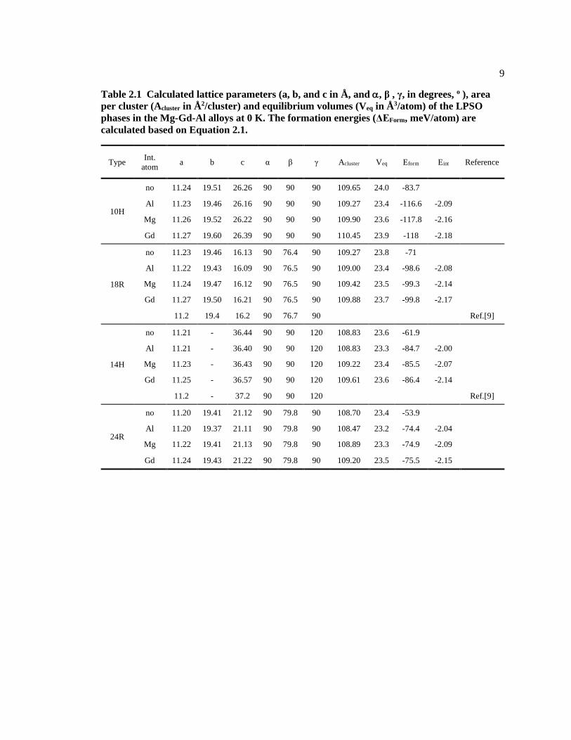
Table 2.1 Calculated lattice parameters (a, b, and c in Å , and , β , γ, in degrees, o ), area
per cluster (Acluster in Å 2/cluster) and equilibrium volumes (Veq in Å 3/atom) of the
LPSO phases in the Mg-Gd-Al alloys at 0 K. The formation energies (ΔEForm,
meV/atom) are calculated based on Equation 2.1. ........................................................... 9
Table 2.2 Calculated lattice features of LPSO structures. 𝑑𝑖𝑛𝑡𝑟𝑎𝑐𝑙𝑢𝑠𝑡𝑒𝑟(Å ) and
𝑑𝑖𝑛𝑡𝑒𝑟𝑐𝑙𝑢𝑠𝑡𝑒𝑟 (Å ) are the 2NN RE-RE intracluster and intercluster
distances, 𝑤cluster(Å ) and ℎcluster(Å ) are the L12 cluster width and height. ............... 11
Table 2.3 Calculated elastic properties of LPSO structures of the Mg-Gd-Al alloys at 0
K, including elastic stiffness constants (Cij's), Young's modulus (E), bulk modulus
(B) from both VRH approach and EOS fitting, and shear modulus (G) from the VRH
approach. The unit for each elastic property is GPa. ....................................................... 13
Table 3.1 Gibbs energies of LPSO end-members obtained from the Debye model, defined
as 𝐺𝐿𝑃𝑆𝑂 − 𝐻𝑆𝐸𝑅 = 𝑎 + 𝑏𝑇 + 𝑐𝑇ln𝑇 + 𝑑𝑇2 + 𝑒𝑇 − 1 + 𝑓𝑇3(J/mole-atom),
where HSER is reference state from SGTE[82]. ................................................................ 32
Table 3.2 Interaction parameters in individual sublattices (kJ/mol-atom). .............................. 34
Table 3.3 Calculated lattice parameters of pure elements in comparison with
computational and experimental data in the literature. .................................................... 35
Table 3.4 Formation energies (Eform in kJ/mole-atom) at 0 K and the scaling factors (s) of
the endmembers, see Equation 3.12, with the elastic constants from Kim et al.[81]. ...... 36
Table 4.1 Slip systems of different crystal structures. ............................................................. 50
Table 4.2 Slip systems at room temperature in BCC metals. ................................................... 53
Table 4.3 Comparison of PN flow stress at 0K with experimental yield stress (𝜏𝑌𝐺) at
low temperatures (4~77 K) as a function of dislocation width. ....................................... 58
Table 4.4 Experimental and calculated ℎ𝑇/ℎ𝑝 and parameter c for various materials. .......... 64
Table 4.5 Comparison of 𝜏𝑃𝑁𝐺 and 𝜏𝑇𝐺 ................................................................................ 68
Table 4.6 Hardness comparison between the present and previous models with slip
systems and elastic properties with S for screw dislocation. ........................................... 74
Table 5.1 The materials’ information used in Figure 5.2 to Figure 5.5. .................................. 95
Table 5.2 Crystal structures and their slip systems. ................................................................. 104
Table 5.3 Self-diffusion activation energy modeling. .............................................................. 106
Table 6.1 The angle (𝜃𝑝) of full and partial dislocations in structures. ................................... 115

xiv
ACKNOWLEDGEMENTS
There are many people that I would like to express my appreciation. More specifically, I
would like to thank four groups of people, without whom this dissertation would not have been
possible: my advisor, my thesis committee members, my lab mates, and my family.
I would like to express thanks to my advisor Dr. Zi-Kui Liu for mainly two aspects. First,
his deep knowledge in thermodynamics inspires me a lot, which now becomes an important part
of my knowledge. Second, he always mentions “critical thinking and communication with others”
that remind me all the times during my study.
In addition, I would like to thank the rest of my committee members, Dr. Adri van Duin,
Dr. Ismaila Dabo, Dr. Hojong Kim and Dr. Laszlo Kecskes for their time, encouragements and
suggestions during serving on my dissertation committee. Especially, I would like to thank to Dr.
Kecskes for the intuitive discussions.
I would like to thank many of my colleagues in the Phases Research Lab for their help
and discussions. Dr. Xuan Liu and Dr. Austin Ross taught me Thermo-Calc and has given many
useful advices since I joined the group. Dr. Shun-Li Shang and Dr. Yi Wang gave me suggestions
on calculation skills. The help and discussions from Dr. Yongjie Hu for dislocation study, Dr. Bi-
Cheng Zhou and Dr. Cassie Marker for thermodynamic modeling, Dr. Richard Otis for
thermodynamic intuition, Dr. Pinwen Guan for calculation details and skills, Brandon Bocklund
for python coding, Jorge Paz Soldan (dynamic duo) for thermodynamic discussions and Matthew
Feurer for DFT-TK help. Their help and discussions are priceless to me.
Lastly, I would like to express my deepest thanks to my lovely wife, Dr. Jungwan Yoon
for being with me always, and to my parents, Donghyune Kim and Kwangsook Ahn for their
supports.
1
Chapter 1
Introduction
1.1 Motivation
Magnesium (Mg) and its alloys are important structural materials in transportation,
aerospace, and consumer electronic industry applications[1]–[3] since they are lightweight.
However, due to their low ductility and low mechanical strength,[4], [5] which stem from a limited
number of slip systems for the hexagonal-close-packed (HCP) crystal structure, their applications
are limited, and many researchers have put great effort to improve the properties of Mg alloys. One
potential solution to overcoming these issues in Mg alloys is to introduce the face-centered-cubic
(FCC) stacking layers with an ABCABC (here, A, B, and C are different close-packed layers)
stacking sequence within the ABABAB HCP stacking layers, i.e., forming the long periodic
stacking ordered (LPSO) phases via TM (Transition Metal)-RE (Rare Earth) solute atoms
clusters[6]–[9]. It has been shown that the presence of LPSO phases improves the tensile strength,
hardness and ductility[10]–[13].
Among various candidates of Mg-TM-RE LPSO phases, Mg-Al-Gd LPSO phases have
obtained considerable attention for two major reasons. First, the alloying elements of Al are much
lighter than Zn or other TM elements. By alloying with Al, the LPSOs will be lighter than other
LPSO phases, that is the major concern for making lightweight structural metal. Second, among
various LPSO phase candidates in Mg-Al-RE ternary systems, only Mg-Al-Gd LPSOs are found
to be stable at finite temperature ranges[14].
In order to investigate the formation of LPSO phases in Mg-Al-Gd system, the phase
stability of LPSOs in Mg-Al-Gd system should be investigated first since the phase equilibria will

2
help to understand the conditions of alloy processing, i.e., temperature and composition ranges.
However, there has been no available thermochemical data for LPSO phases, and no research on a
thermodynamic model with solubilities of LPSO phases in the Mg-Al-Gd system. Furthermore, in
order to predict mechanical properties of LPSOs, i.e. hardness, a unified model which enables to
predict hardness not only for pure metals but also for complex compounds such as LPSO phases,
should be developed. So far, there is no hardness model for metals and alloys other than the
empirical expression of 𝐻𝑣 = 3𝜎𝑌 . Overall, although considerable efforts have been made to
understand and improve phase stability and mechanical properties of LPSO phases, there is still
lack of clear and systematic understanding of the relationship between the structure and the
resulting phase equilibria and mechanical properties, i.e., hardness, which will be the focus of the
present work.
1.2 Overview
The ultimate goal of this dissertation is to give a comprehensive description of the phase
equilibria of LPSO phases in Mg-Al-Gd system by a combined CALPHAD-DFT methodology,
and is to predict the mechanical properties of LPSOs by modeling hardness of polycrystalline
materials which implemented plastic deformations into the model. To achieve these goals, the
related methodologies are developed in the following chapters. Specifically, in Chapter 2, the
elastic properties of LPSO phases in Mg-Al-Gd system such as elastic stiffness constants were
calculated based on the first-principles calculations. In addition to this, orientation dependent shear
and Young’s moduli were discussed. In Chapter 3, the phase equilibria of the Mg-Al-Gd system
with LPSO phases were modeled by a combined CALPHAD-DFT methodology. Due to the lack
of sufficient experimental data, first-principles calculations played an important role in modeling
this system.
3
In Chapter 4, a Vickers hardness model for polycrystalline materials was developed since
there is no available model for predicting hardness of any metallic phases including LPSO phases.
The Vickers hardness model considers both elastic and plastic deformation of materials by
implementing Peierls-Nabarro flow stress in order to capture the plastic deformation of materials.
The developed hardness model agrees well with experimental results of metals and ceramics which
indicates the reliability of the model is from below 0.1 GPa to over 100 GPa. Especially the active
slip system as well as melting temperature and elastic properties (shear and bulk moduli and
Poisson’s ratio) played a significant role in determining materials’ hardness. In Chapter 5, a
temperature-dependent hardness model was developed by implementing diffusion mechanisms
such as dislocation (pipe), mono- and di-vacancy diffusions into the hardness model which was
developed in Chapter 4, since LPSOs are intermediate temperature phases. Especially, the modeling
of the activation energy for self(mono-vacancy)-diffusion, which is based on the earlier belief of
the Van Liempt rule, helped to simplify the model. This chapter was explained by the factors that
affect the hardness of materials as a function of temperature with some examples. The developed
temperature-dependent hardness model agrees well with 16 examples including FCC, BCC, HCP
and ceramic materials. In Chapter 6, the twin layer dependent hardness model was developed since
LPSO phases are layered structures. This chapter discussed how the active slip systems are changed
by the twin boundaries. This model has great agreement with experimental results of carbon
diamond cubic and FCC metals. In Chapter 7, the hardness of LPSOs in Mg-Al-Gd ternary systems
was predicted based on the hardness models developed in Chapters 4-6. In Chapter 8, the
conclusions were drawn and the future works were discussed.

4
Chapter 2
Elastic Properties of Long Periodic Stacking Ordered Phases in Mg-Al-Gd
Alloys: A First-Principles Study
2.1 Introduction
It has been shown that the presence of LPSO phases improves the tensile strength and
ductility[10]. For example, the Mg97Zn1Y2 (at.%) alloy, which includes the LPSO phase, reaches a
high yield strength of 480-610 MPa and an elongation of 5~16%, respectively[10]. While it is
known that such enhanced mechanical properties result from LPSO phases as well as grain
refinement,[11]–[13] the underlying mechanism of this phenomenon has not yet been fully
explained due to the plastic behavior of LPSOs. Since the mechanical properties can be estimated
from slip systems and elastic properties such as Poisson’s ratio and shear modulus[15], [16], the
elastic properties are one of the important factors in order to understand plastic deformations.
In order to understand the elastic properties of LPSOs, it is crucial to clarify the effects of
the crystal structures of LPSOs, especially the ordering of solute atoms in LPSOs, since the elastic
properties of LPSOs are largely affected by the nature of bonding, which is determined by the
crystal structures. Reported LPSO phases in the Mg-TM-RE ternary systems consist of 5-8 atomic
layers in the structural block (SB), a unit with the minimum number of stacking layers that includes
one set of stacking faults[6]–[8], [17]–[19]. For example, there are six layers in the 18R LPSO SB,
and seven layers in the 14H LPSO SB. These SBs are also referred to as the 10H, 18R, 14H, and
24R poly-types according to the Ramsdell notation[9], [20], [21], where the number represents total
layers in the repeating unit cell, and the letters H and R represent the hexagonal and rhombohedral
symmetries, respectively. Moreover, the solute atoms located in the 4-continued atomic layers and

5
these solute atoms form a specific in-plane ordering of the L12 cluster[6]–[9]. Kimizuka et al.[22]
verified the formation of the L12-type clusters in terms of Gd and Al in the Mg-Gd-Al system, using
the cluster expansion method. From the images, several investigators[17]–[19], [23] used scanning
transmission electron microscopy (STEM) to verify the L12 clusters of solute atoms in the stacking
fault regions of the LPSO phase and describe the two-dimensional (2D) close-packed in-plane
ordering of these L12 clusters. Furthermore, an interstitial atom (Mg, RE, or TM) at the center of
the L12 cluster has been observed in the Mg-Y-Zn system through STEM images[18], and
suggested by density functional theory (DFT) based first-principles calculations[24].
Furthermore, it is also crucial to clarify the effect of the L12 cluster interactions and the
contribution of the interstitial atom in the cluster since the L12 cluster is the key lattice feature of
the crystal structures of LPSOs. Recently, Kimizuka et al. described the cluster interaction of LPSO
phases with or without interstitial atom and the changes of RE-RE intracluster and intercluster
bonding distances[25]. The intracluster and intercluster distances represent the average 2nd nearest
neighbor (2NN) distances of RE atoms within and between the clusters, respectively. The smaller
cluster interaction undergoes the larger contraction of RE-RE intracluster bonding distance among
the L12 clusters with an interstitial atom. The intracluster bonding distance is related to the size of
cluster. Furthermore, Tane et al. reported there is a relationship between cluster interaction energy
or cluster density and elastic properties such as Young’s modulus and shear modulus[26]. The
findings of the previous literature imply that changes of the bonding environment around the L12
cluster should influence the elastic properties of LPSO phases via the changes of cluster interaction
or cluster density.
The present work aims to study the elastic properties of the Mg-Gd-Al LPSO phases (10H,
18R, 14H, and 24R) using first-principles calculations, where all of the possible L12-type clusters
with and without interstitial atoms are considered. The interstitial atoms Mg, Gd, and Al are

6
denoted as Mg-int., Gd-int. and Al-int., respectively. The predicted elastic properties of the LPSO
phases are interpreted by examining atomic bonding environments around the L12 clusters and
electronic structures.
2.2 Computational Methods
The crystal structure of 14H LPSO is P63/mcm, proposed by Egusa and Abe[23] based on
various theoretical and experimental results[17], [19], [23]. Space groups 18R and 24R LPSOs are
designated as C2/m[6], [18], [19], [23]. The crystal structures of 10H LPSO phase is designated as
Cmce, which was suggested by Kishida et al.[18] according to the stable LPSO phase in the Mg-
Y-Zn system. In order to describe the L12-type clusters in the DFT calculations, the number of
atoms in each LPSO phase are 240 (10H LPSO), 168 (14H LPSO), 144 (18R LPSO), and 192 (24R
LPSO), respectively, associated with the Gd and Al clustering in the stacking fault layers[18], [23].
First-principles calculations are conducted by using the Vienna Ab-initio Simulation
Package (VASP) [27], [28]. Electron-ion interactions are described by the projector augmented-
wave (PAW) method[29]. In order to describe the electron interactions including exchange and
correlation, the generalized gradient approximation (GGA) as implemented by Perdew, Burke, and
Ernzerhof (PBE)[30] is used. Plane wave cutoff energies of 350 eV are consistently used for all the
calculations, which are 1.3 times higher than the recommended ones by the VASP[31]. For HCP-
Mg with 2 atoms in the supercell, the 29 × 29 × 16 Γ-centered k-point grids are implemented. For
the crystal structures of LPSO phases, we use the 3 × 5 × 2 (10H LPSO with 240 atoms in the
supercell), 6 × 6 × 2 (14H LPSO with 168 atoms), 6 × 3 × 3 (18R LPSO with 144 atoms), and 3 ×
2 × 2 (24R LPSO with 192 atoms) Γ-centered k-point grids, respectively. The k-mesh guarantees
errors below 0.1 meV/atom (0.2 meV/atom for 24R LPSO due to the computational resource
limitations). The f-electrons of the Gd element are treated as core electrons, an approximation that

7
has shown to produce accurate thermodynamic properties for lanthanide-containing structures[32]–
[35]. After full relaxations, a final static calculation using the tetrahedral method with Blöch
corrections[36] is applied to ensure the accuracy of total energy. The energy convergence criterion
of the electronic self-consistency is set as 10-6 eV/atom for all of the calculations. The contour plots
of the differential charge density are generated using VESTA[37], [38].
The formation energies and the contribution of interstitial atom of LPSOs[14] are
calculated by Equation 2.1 and Equation 2.2, and listed in Table 2.1.
Equation 2.1 𝑬𝒇𝒐𝒓𝒎(𝑳𝑷𝑺𝑶) = 𝑬(𝑳𝑷𝑺𝑶) − 𝟏
𝑵∑ 𝑵𝒊𝑬𝒊𝒊
where Ei is the total energy of stable bulk state of species per atom of species i and Ni is the number
of atom of species i.
Equation 2.2 ∆𝑬𝒊𝒏𝒕𝒊 =
𝑬(𝑳𝑷𝑺𝑶+𝑵𝒊×𝒊𝒏𝒕)−𝑬(𝑳𝑷𝑺𝑶)− 𝑵𝒊𝑬𝒊
𝑵𝒊
In the present work, elastic stiffness constants are predicted at 0 K via DFT-based first-
principles calculations in terms of the stress–strain method [39]. To determine elastic constants for
a crystal from first-principles and Hooke’s law, a set of strains, expressed in Voigt notation with 𝜀
= (𝜀1, 𝜀2, 𝜀3, 𝜀4, 𝜀5, 𝜀6) (where 𝜀1, 𝜀2, 𝑎𝑛𝑑 𝜀3 are the normal strains and the others are the shear
strains), are placed on a crystal with lattice vectors R,
Equation 2.3 𝑹 = (
𝒂𝟏 𝒂𝟐 𝒂𝟑𝒃𝟏 𝒃𝟐 𝒃𝟑𝒄𝟏 𝒄𝟐 𝒄𝟑
)
After deformation, the resulting lattice vectors, R’, can be expressed as
Equation 2.4 𝑹′ = 𝑹(
𝟏 + 𝜺𝟏 𝝐𝟔/𝟐 𝝐𝟓/𝟐𝝐𝟔/𝟐 𝟏 + 𝜺𝟐 𝝐𝟒/𝟐𝝐𝟓/𝟐 𝝐𝟒/𝟐 𝟏 + 𝜺𝟑
)
Correspondingly, stresses 𝜎 = (𝜎1, 𝜎2, 𝜎3, 𝜎4, 𝜎5, 𝜎6) for each set of strains can be calculated
using first-principles to determine the 6 × 6 elastic stiffness constants matrix (C),
8
Equation 2.5
(
𝝈𝟏,𝟏𝝈𝟐,𝟏𝝈𝟑,𝟏𝝈𝟒,𝟏𝝈𝟓,𝟏𝝈𝟔,𝟏
…
𝝈𝟏,𝒏𝝈𝟐,𝒏𝝈𝟑,𝒏𝝈𝟒,𝒏𝝈𝟓,𝒏𝝈𝟔,𝒏)
=
(
𝑪𝟏𝟏𝑪𝟐𝟏𝑪𝟑𝟏𝑪𝟒𝟏𝑪𝟓𝟏𝑪𝟔𝟏
𝑪𝟏𝟐 𝑪𝟐𝟐𝑪𝟑𝟐𝑪𝟒𝟐𝑪𝟓𝟐𝑪𝟔𝟐
𝑪𝟏𝟑𝑪𝟐𝟑𝑪𝟑𝟑𝑪𝟒𝟑𝑪𝟓𝟑𝑪𝟔𝟑
𝑪𝟏𝟒𝑪𝟐𝟒𝑪𝟑𝟒𝑪𝟒𝟒𝑪𝟓𝟒𝑪𝟔𝟒
𝑪𝟏𝟓𝑪𝟐𝟓𝑪𝟑𝟓𝑪𝟒𝟓𝑪𝟓𝟓𝑪𝟔𝟓
𝑪𝟏𝟔𝑪𝟐𝟔𝑪𝟑𝟔𝑪𝟒𝟔𝑪𝟓𝟔𝑪𝟔𝟔)
(
𝜺𝟏,𝟏𝜺𝟐,𝟏𝜺𝟑,𝟏𝜺𝟒,𝟏𝜺𝟓,𝟏𝜺𝟔,𝟏
…
𝜺𝟏,𝒏𝜺𝟐,𝒏𝜺𝟑,𝒏𝜺𝟒,𝒏𝜺𝟓,𝒏𝜺𝟔,𝒏)
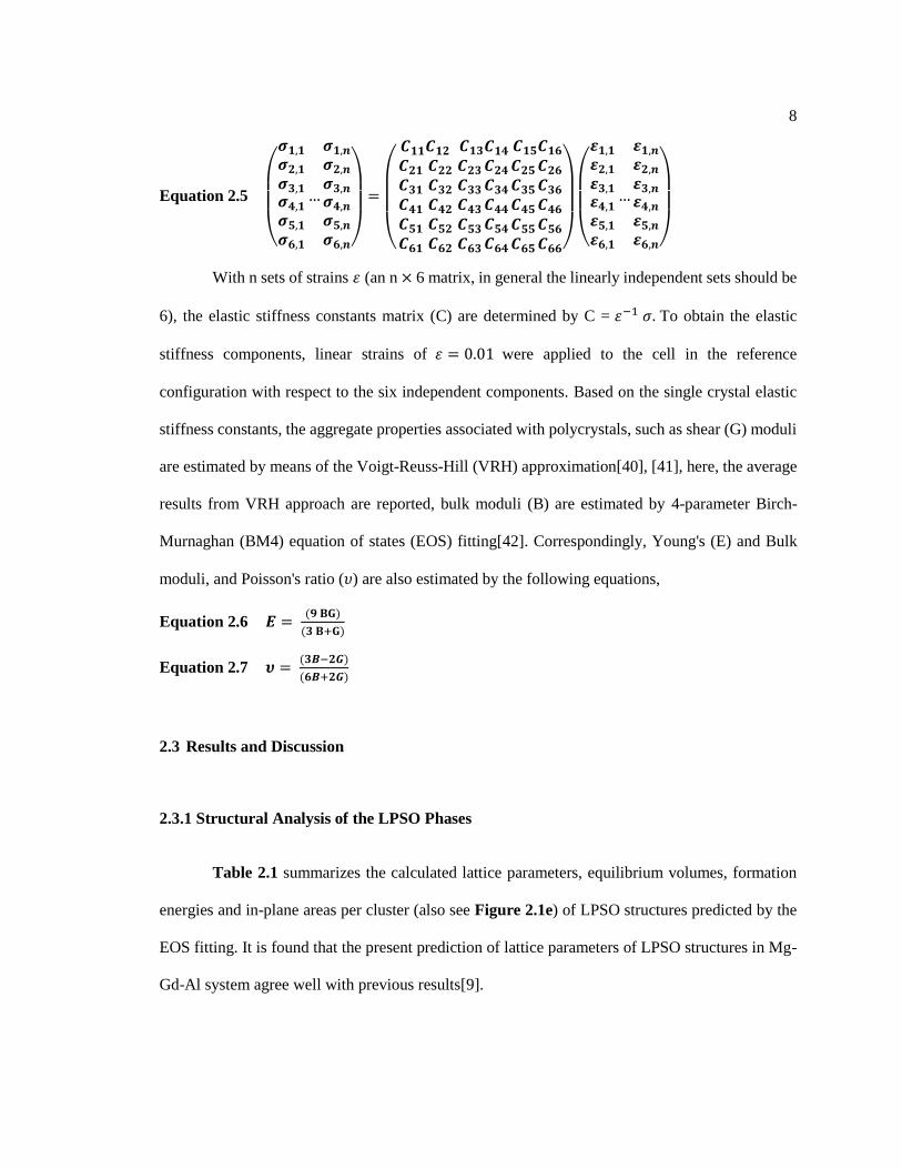
With n sets of strains 𝜀 (an n × 6 matrix, in general the linearly independent sets should be
6), the elastic stiffness constants matrix (C) are determined by C = 𝜀−1 𝜎. To obtain the elastic
stiffness components, linear strains of 𝜀 = 0.01 were applied to the cell in the reference
configuration with respect to the six independent components. Based on the single crystal elastic
stiffness constants, the aggregate properties associated with polycrystals, such as shear (G) moduli
are estimated by means of the Voigt-Reuss-Hill (VRH) approximation[40], [41], here, the average
results from VRH approach are reported, bulk moduli (B) are estimated by 4-parameter Birch-
Murnaghan (BM4) equation of states (EOS) fitting[42]. Correspondingly, Young's (E) and Bulk
moduli, and Poisson's ratio (𝜐) are also estimated by the following equations,
Equation 2.6 𝑬 = (𝟗 𝐁𝐆)
(𝟑 𝐁+𝐆)
Equation 2.7 𝝊 = (𝟑𝑩−𝟐𝑮)
(𝟔𝑩+𝟐𝑮)
2.3 Results and Discussion
2.3.1 Structural Analysis of the LPSO Phases
Table 2.1 summarizes the calculated lattice parameters, equilibrium volumes, formation
energies and in-plane areas per cluster (also see Figure 2.1e) of LPSO structures predicted by the
EOS fitting. It is found that the present prediction of lattice parameters of LPSO structures in Mg-
Gd-Al system agree well with previous results[9].
9
Table 2.1 Calculated lattice parameters (a, b, and c in Å , and , β , γ, in degrees, o ), area
per cluster (Acluster in Å 2/cluster) and equilibrium volumes (Veq in Å 3/atom) of the LPSO
phases in the Mg-Gd-Al alloys at 0 K. The formation energies (ΔEForm, meV/atom) are
calculated based on Equation 2.1.
Type Int.
atom a b c α β γ Acluster Veq Eform Eint Reference
10H
no 11.24 19.51 26.26 90 90 90 109.65 24.0 -83.7
Al 11.23 19.46 26.16 90 90 90 109.27 23.4 -116.6 -2.09
Mg 11.26 19.52 26.22 90 90 90 109.90 23.6 -117.8 -2.16
Gd 11.27 19.60 26.39 90 90 90 110.45 23.9 -118 -2.18
18R
no 11.23 19.46 16.13 90 76.4 90 109.27 23.8 -71
Al 11.22 19.43 16.09 90 76.5 90 109.00 23.4 -98.6 -2.08
Mg 11.24 19.47 16.12 90 76.5 90 109.42 23.5 -99.3 -2.14
Gd 11.27 19.50 16.21 90 76.5 90 109.88 23.7 -99.8 -2.17
11.2 19.4 16.2 90 76.7 90 Ref.[9]
14H
no 11.21 - 36.44 90 90 120 108.83 23.6 -61.9
Al 11.21 - 36.40 90 90 120 108.83 23.3 -84.7 -2.00
Mg 11.23 - 36.43 90 90 120 109.22 23.4 -85.5 -2.07
Gd 11.25 - 36.57 90 90 120 109.61 23.6 -86.4 -2.14
11.2 - 37.2 90 90 120 Ref.[9]
24R
no 11.20 19.41 21.12 90 79.8 90 108.70 23.4 -53.9
Al 11.20 19.37 21.11 90 79.8 90 108.47 23.2 -74.4 -2.04
Mg 11.22 19.41 21.13 90 79.8 90 108.89 23.3 -74.9 -2.09
Gd 11.24 19.43 21.22 90 79.8 90 109.20 23.5 -75.5 -2.15

10
Figure 2.1 The LPSO structures of 10H (a), 18R (b), 14H (c), and 24R (d) together with the
in-plane L12 cluster ordering (e) and the Gd8Al6 L12 cluster with an interstitial (int.) atom
Gd, Mg or Al (f). Blue box stands for the unit cell of each LPSO structures and the red bracket
with SB stands for structural block for each LPSO structure. 𝒅𝒊𝒏𝒕𝒓𝒂𝒄𝒍𝒖𝒔𝒕𝒆𝒓 and 𝒅𝒊𝒏𝒕𝒆𝒓𝒄𝒍𝒖𝒔𝒕𝒆𝒓 stands for the 2NN RE-RE intracluster and intercluster distances, 𝒘𝐜𝐥𝐮𝐬𝐭𝐞𝐫 and 𝒉𝐜𝐥𝐮𝐬𝐭𝐞𝐫 stands
for the L12 cluster width and height.
It can be seen that the lattice parameters of all LPSO supercell structures (larger than 11.20
Å ) are larger than those of HCP Mg, which corresponds to 11.07 Å (2√3 𝑎𝑀𝑔with aMg being 3.196
Å ). This represents that in the normal stacking layers (ABAB…), Mg atoms endure the tensile
stresses along the [1120] and [1010] directions due to the L12 clusters when it is compared with
HCP Mg structure. Among the LPSOs, the lattice parameter, a, is the largest (11.24 Å ) for the 10H

11
LPSO phase and decreases as the number of layers in SB increases to 11.20 Å for the 24R LPSO
phase. Since the distance between clusters is proportional to the lattice parameter, the number of
clusters in basal plane increases as the number of layers in SB increases. Furthermore, we also
examined the lattice relaxation of L12 clusters in the LPSO phases, since the cluster interaction can
be quantified by the changes of cluster dimensions. Kimizuka et al.[25] examined the 2NN RE-RE
bonding distances (intercluster and intracluster 2NN RE-RE distances as listed in Table 2.2) and
their effects on the intercluster interactions. Based on their work, it is also found that the types of
the interstitial atom induce changes of 2NN RE-RE bonding distances and intercluster interactions.
In this work, we examine the lattice relaxations of L12 cluster such as the in-plane area per cluster,
Acluster, the L12 cluster width (𝑤cluster: body diagonal distance between Gd atoms within stacking
fault region), and the L12 cluster height (ℎcluster: the distance between top and bottom Gd atoms
in the L12 cluster), listed in Table 2.2. It is found that the cluster with smaller interstitial atom, Al,
undergoes further inward contraction of the cluster.
Table 2.2 Calculated lattice features of LPSO structures. 𝒅𝒊𝒏𝒕𝒓𝒂𝒄𝒍𝒖𝒔𝒕𝒆𝒓 (Å ) and 𝒅𝒊𝒏𝒕𝒆𝒓𝒄𝒍𝒖𝒔𝒕𝒆𝒓 (Å ) are the 2NN RE-RE intracluster and intercluster
distances, 𝒘𝐜𝐥𝐮𝐬𝐭𝐞𝐫(Å ) and 𝒉𝐜𝐥𝐮𝐬𝐭𝐞𝐫(Å ) are the L12 cluster width and height.
Int.
type no no no no Al Al Al Al Mg Mg Mg Mg Gd Gd Gd Gd
SB 5 6 7 8 5 6 7 8 5 6 7 8 5 6 7 8
𝑑𝑖𝑛𝑡𝑟𝑎𝑐𝑙𝑢𝑠𝑡𝑒𝑟 4.1
0
4.1
2
4.1
4
4.1
3
4.0
8
4.1
0
4.1
1
4.1
0
4.1
0
4.1
2
4.1
2
4.1
1
4.1
3
4.1
6
4.1
6
4.1
4
𝑑𝑖𝑛𝑡𝑒𝑟𝑐𝑙𝑢𝑠𝑡𝑒𝑟 5.0
9
5.0
6
5.0
3
5.0
3
5.0
9
5.0
7
5.0
6
5.0
6
5.1
0
5.0
7
5.0
6
5.0
7
5.1
0
5.0
9
5.0
9
5.0
8
𝑤cluster 7.13
7.16
7.19
7.17
7.12
7.12
7.13
7.12
7.14
7.15
7.15
7.13
7.18
7.19
7.19
7.16
ℎcluster 7.2
7
7.2
6
7.2
5
7.2
9
7.1
7
7.1
6
7.1
5
7.1
7
7.2
2
7.2
1
7.1
8
7.2
1
7.2
7
7.2
9
7.2
4
7.2
9

12
2.3.2 Elastic Properties of the LPSO Phases
Calculated elastic properties Cij, B(EOS), B(VRH), G, E and 𝜈 (Poisson ratio) of the LPSO
phases are summarized in Table 2.3. For the comparison reason, the calculated elastic stiffness
matrix of 10H LPSO supercell and 18R and 24R LPSO supercell, orthorhombic and monoclinic
crystal structures, respectively, are converted based on hexagonal symmetry since 18R and 24R
LPSO supercells used in this study are based on Niggli reduced cell from hexagonal symmetry[43],
[44]. The 10H LPSO supercell used in this study shows lower formation energy than other 10H
LPSO supercells[18]. However, the complete elastic stiffness matrixes of 10H, 18R and 24R LPSO
phases are listed in Appendix A.
Since no existing elastic constants are available for the Mg-Gd-Al LPSO phases, first, we
compare the present elastic constants of HCP Mg from first-principles calculations with
experiments and other calculations[45]–[48]. The calculated elastic moduli of HCP Mg are in the
range of experiments or have small differences, less than 1.6% except for C12 which is 5.5%
different from experiments[46], also, bulk and Young’s moduli are in the range of
experiments[46]–[48]. Second, the elastic stiffness matrix of the Mg-Y-Zn 18R LPSO phases are
calculated and compared with experimental results[26], [47], [49] and other theoretical
calculations[50]. Experimental elastic properties include nanoindentation measurements using
resonant ultrasound spectroscopy combined with electromagnetic acoustic resonance (65.0±1.4
GPa along the [0001] and 54.0±0.6 GPa along the [1120] direction for Young’s modulus)[26], and
microindentation (66.7±4.9 GPa for Young’s modulus)[49]. Our calculations are in good
agreement with these experiments with ~3 % error, especially for the Mg-Y-Zn 18R LPSO phase
where the experimental data were collected at 5.5 K[26].
In order to investigate the prevailing lattice distortion induced by solute atoms in L12
cluster, Figure 2.2 plots the bulk moduli from elastic calculations (VRH) and EOS as a function of

13
the number of layers in the SB which are also reported in Table 2.3. For a reliable interpretation of
the bulk moduli results, we reported bulk moduli from both methods to see the trends. Both results
have similar trends, except the 10H LPSO. The discrepancy is due to the elastic calculation method
which uses smaller deformation ranges than that of EOS fitting and calculated from a fixed volume.
As shown in Figure 2.2a, with increasing the number of layers in the SB, bulk moduli from EOS
fitting and from VRH of the LPSO decrease slightly. In addition, for the same interstitial atom in
various LPSO phases, this trend is even more clearly shown. The bulk modulus increases from 40.4
GPa (24R) to 42.1 GPa (10H) for LPSO phase with Al-int. with decreasing the number of layers in
the SB. The previous studies indicated that bulk moduli are inversely correlated to equilibrium
volumes of pure elements[42] ( 𝐵 = 20422𝑉−1.868) and also in dilute Ni- and Mg-based
alloys[51], [52]. Since the cluster density, defined as the number of clusters in a unit volume (𝜌𝑉 =
𝑁𝑐𝑙/𝑉 = 2(𝑜𝑟 4 𝑓𝑜𝑟 10𝐻)/𝑠𝑢𝑝𝑒𝑟𝑐𝑒𝑙𝑙 𝑣𝑜𝑙𝑢𝑚𝑒), this trend can be rephrased as the denser the L12
cluster density is, the larger the bulk moduli will be.
Table 2.3 Calculated elastic properties of LPSO structures of the Mg-Gd-Al alloys at 0 K,
including elastic stiffness constants (Cij's), Young's modulus (E), bulk modulus (B) from
both VRH approach and EOS fitting, and shear modulus (G) from the VRH approach. The
unit for each elastic property is GPa.
Type System Int. C11 C33 C12 C13 C44 C66 BVRH BEOS G E 𝜈 Ref.
HCP
Mg
61.3 66.2 27.6 21.5 18.7 16.6 36.7 36.5 18.5 47.6 0.283 TW 59.3 61.4 25.9 21.6 16.3 - - - - [45]
59.5 61.6 25.9 21.8 16.4 - 35.6 17.3 44.6 [48]
63.5 66.5 25.9 21.7 18.4 18.7 36.9 19.4 49.5 [46]
- - - - - - - - 48
±4 [47]
10H
Mg-Gd-
Al no 75.6 87.4 27.7 17.5 24.3 22.4 40.8 37.8 25.4 63.1 0.239 TW
Mg-Gd-
Al Al 80.1 91.6 28.9 17.6 25.2 26.0 42.1 41.9 27.5 67.8 0.230 TW
Mg-Gd-
Al
M
g 78.9 90.4 28.8 17.5 23.8 24.6 41.9 41.5 26.3 65.2 0.237 TW
Mg-Gd-
Al Gd 72.0 90.3 29.5 19.1 23.9 19.7 41.7 41.2 22.3 56.7 0.268 TW
18R Mg-Gd-
Al no 73.3 84.3 27.7 15.3 25.2 22.0 38.8 37.7 25.5 62.8 0.226 TW

14
Mg-Gd-
Al Al 78.8 89.0 26.7 18.1 26.5 25.1 41.6 40.9 27.5 67.6 0.227 TW
Mg-Gd-
Al
M
g 77.6 88.9 27.2 17.8 26.9 23.8 41.4 40.6 27.1 66.8 0.228 TW
Mg-Gd-
Al Gd 75.8 87.9 28.4 18.0 24.4 22.0 41.3 40.4 25.3 62.9 0.242 TW
Mg-Y-
Zn no 70.4 85.3 30.1 19.4 22.9 20.0 40.5 23.2 58.5 0.256 TW
Mg-Y-
Zn Zn 69.8 84.6 32.4 19.5 21.8 19.4 40.6 22.5 56.9 0.263 TW
Mg-Y-
Zn
M
g 70.6 85.4 32.3 19.1 22.9 20.2 40.6 23.4 58.9 0.256 TW
Mg-Y-
Zn Y 70.7 84.3 30.4 19.7 22.9 18.4 41.0 22.5 57.1 0.263 TW
Mg-Y-
Zn NA
72.5
±0.
7
80.0
±1.
8
-
18.9
±1.
1
23.5
±0.
3
21.2
±0.
3
- -
73.0
±1.
9
58.4
±0.
3
[26]
Mg-Y-
Zn NA - - - - - - - -
66.7
±4.
9
[49]
Mg-Y-
Zn NA
67.7
±1.
0
72.9
±2.
0
28.3
±1.
1
19.5
±0.
8
21.5
±0.
3
19.7
±0.
3
38.0
±0.
7
65.0
±1.
4
54.0
±0.
6
[53]
Mg-Y-
Zn NA
68.1
±1.
0
67.2
±0.
9
21.6
±0.
7
24.0
±0.
8
20.6
±0.
2
23.2
±0.
2
-
21.8
±0.
1
54.9
±0.
4
[53]
Mg-Y-
Zn no 71.6 82.0 28.7 19.7 23.2 - [26] +
Mg-Y-
Zn
M
g 79.5 87.8 23.1 16.7 25 - 40 28.1 68.4 [50] +
Mg-Y-
Zn
M
g 77 82.3 18.2 15.8 26.6 - 37.3 28.9 69 [50] *
14H
Mg-Gd-
Al no 71.1 83.8 27.3 16.4 26.4 22.5 38.6 37.6 25.9 63.5 0.222 TW
Mg-Gd-
Al Al 75.1 87.4 28.2 17.9 26.0 23.5 40.6 40.2 26.4 65.2 0.230 TW
Mg-Gd-
Al
M
g 72.5 86.1 29.7 18.2 25.7 21.0 40.5 40.0 25.0 62.3 0.240 TW
Mg-Gd-
Al Gd 72.9 85.9 29.3 18.2 24.2 21.9 40.3 39.9 24.8 61.8 0.242 TW
24R
Mg-Gd-
Al no 73.1 82.9 24.5 15.7 24.6 21.3 38.5 37.5 24.9 61.5 0.229 TW
Mg-Gd-
Al Al 77.4 85.1 25.5 17.6 25.2 25.0 40.4 39.8 26.7 65.6 0.227 TW
Mg-Gd-
Al
M
g 75.4 85.7 27.4 17.1 26.5 24.0 40.0 39.7 26.8 65.8 0.224 TW
Mg-Gd-
Al Gd 72.9 86.6 28.8 17.1 28.1 20.4 40.2 39.6 25.9 63.9 0.230 TW
+ VASP and * SIESTA calculations, TW-this work, NA-did not mentioned

15
Figure 2.2 Calculated bulk moduli of the LPSO phases with respect to number of layers in
structural block; (a) bulk modulus from EOS fitting and (b) bulk modulus from VRH
approach. Red dash lines indicate the bulk and shear moduli of HCP Mg.
The introduction of an interstitial atom in the LPSO increases the bulk moduli. For
example, the bulk modulus (VRH) of 18R LPSO is 38.8 GPa while that of 18R LPSO with Al-int.
is 41.6 GPa. This could be explained by the change of bonding environment. Particularly, the
introduction of an interstitial atom in the L12 cluster creates new bonding within the L12 cluster.

16
This can be confirmed by the change of density of the L12 cluster due to the lattice relaxation and
the energy contribution by the interstitial atom in L12 cluster. The density of the cluster with an
interstitial atom (e.g., Gd8Al7, Gd9Al6 or Gd8Al6Mg) is higher than that of cluster without interstitial
atom (e.g. Gd8Al6) due to the atomic volume reduction by inserting an interstitial atom. Especially
the case of Al interstitial LPSO, by inserting an Al-int. into the cluster, the cluster width changes
from 7.16 Å to 7.12 Å and the cluster height changes from 7.26 Å to 7.16 Å for 18R and also, the
intracluster 2NN RE-RE distance (𝑑𝑖𝑛𝑡𝑟𝑎𝑐𝑙𝑢𝑠𝑡𝑒𝑟) also reduces from 4.12 Å to 4.10 Å (Table 2.2).
This results in a smaller equilibrium volume per atom and higher bulk moduli for the LPSO with
an interstitial atom. Thus, the slope of the bulk moduli of the interstitial LPSO is affected by the
equilibrium volume per atom which is originated from the local density of the L12 cluster.
The effects of the stacking sequence of the LPSO phases on the elastic properties were
examined in terms of the formation energy per unit volume. Figure 2.3 shows the bulk moduli
comparison between elastic calculations with VRH method and from EOS fitting, and Young’s
moduli along [0001] direction (E[0001]) in terms of formation energy per unit volume. In Figure
2.3a, both bulk moduli have the similar trends that they increased almost linearly with decreasing
formation energy per unit volume, although LPSO structures without an interstitial atom have a
different slope from those with an interstitial atom. The slope difference originates from the
changes of the bonding nature around L12 clusters. The bulk modulus discrepancy between elastic
calculations with VRH and EOS fitting is from the types of applied pressure, although the bulk
moduli from both methods should be the same in principle. For example, the bulk modulus from
EOS fitting is calculated from the second derivative of energy over isotropic volume changes, while
that from VRH is an average value from energy with applied anisotropic pressure. Since we have
used 9 volumes for EOS fitting, the bulk modulus from EOS fitting may be more accurate.
Furthermore, E[0001] of LPSO structures increased almost linearly with decreasing formation energy
per unit volume, shown in Figure 2.3b. It is observed that the formation energy per unit volume

17
decreases with the increasing number of layers in SB, i.e. the addition of Mg layers between clusters
along [0001] direction, resulting in lower cluster density along [0001] direction and smaller E[0001].
Therefore, the Young’s modulus along [0001] direction, E[0001], related to the formation energy of
LPSO due to the atomic bonding changes between the stacking layers, especially the cluster density
changes along [0001] direction.
Figure 2.3 (a) comparison of bulk moduli both from VRH and EOS fitting as a function of
formation energies of LPSOs, and (b) Young’s modulus along [0001] direction trend as a
function of volumetric formation energies (𝑬𝒇/𝑽) of LPSOs.
Based on the present calculations shown in Figure 2.4, elastic constants such as C11, C33,
C44, and C66 of the LPSOs are larger than those of HCP Mg due to the introduction of solute atoms
and the formation of L12 cluster. The elastic stiffness component of C33 shows a linear trend with
the number of layers in the structural block (SB) as depicted in Figure 2.4b. The cluster density
decreases with the increasing number of layers in SB. This is related to the bonds in the [0001]
direction, which lead to the decrease of C33 shown in Figure 2.4b. For example, C33 of LPSO
without an interstitial atom decreased from 87.4 to 82.9 GPa. Furthermore, C11 (Figure 2.4a) is
mainly related to the atomic bonds within the basal plane. As Kimizuka et al.[54] described, 2NN
RE-RE intercluster and intracluster bonding distances are related to cluster interactions, which
indicates that the C11 may be determined by the competition between intercluster and intracluster
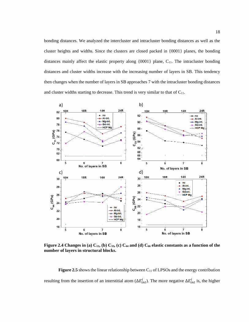
18
bonding distances. We analyzed the intercluster and intracluster bonding distances as well as the
cluster heights and widths. Since the clusters are closed packed in {0001} planes, the bonding
distances mainly affect the elastic property along {0001} plane, C11. The intracluster bonding
distances and cluster widths increase with the increasing number of layers in SB. This tendency
then changes when the number of layers in SB approaches 7 with the intracluster bonding distances
and cluster widths starting to decrease. This trend is very similar to that of C11.
Figure 2.4 Changes in (a) C11, (b) C33, (c) C44 and (d) C66 elastic constants as a function of the
number of layers in structural blocks.
Figure 2.5 shows the linear relationship between C11 of LPSOs and the energy contribution
resulting from the insertion of an interstitial atom (∆𝐸𝑖𝑛𝑡𝑖 ). The more negative ∆𝐸𝑖𝑛𝑡
𝑖 is, the higher

19
C11 becomes. This trend was valid for LPSOs with the interstitial atom, except the 10H LPSO with
the interstitial Gd atom, probably due to the high out-of-plane interaction between L12 clusters.
This linear relationship between the ∆𝐸𝑖𝑛𝑡𝑖 and C11 mainly originates from the changes of the
bonding distances around the L12 cluster (listed in Table 2.2) because the ∆𝐸𝑖𝑛𝑡𝑖 stems from the
bonding environment change around the L12 cluster due to the interstitial atom. For example, the
∆𝐸𝑖𝑛𝑡𝐴𝑙 increased from -2.09 meV/int (10H) to -2.00 meV/int (14H), as the intracluster distance
increased from 4.08Å (10H) to 4.11Å (14H). This trend of ∆𝐸𝑖𝑛𝑡𝑖 as a function of the number of
layers in the SB is very similar to that of C11.
Figure 2.5 Comparison between C11 and the energy contribution of interstitial atom in L12
cluster.
Moreover, it is found that C66 shows a similar trend with respect to that of the C11. C66 is
determined by the shear force along [1010] or [2110] direction while C11 is determined by the
tensile or compressive force along [10 1 0] or [21 1 0] direction. Both the elastic stiffness
components, C11 and C66, should be related to all the bonds along that direction. Since elastic

20
properties are related to cluster interaction or cluster density, C11 and C66 are related to the
intercluster and intracluster bonding distances. Figure 2.6 shows that the relationship between the
elastic stiffness components, the C11 and C66, and the L12 cluster width. This represents that the
smaller cluster width indicates the larger C11 and C66.
Figure 2.6 Relationship of L12 cluster width with (a) C11, and (b) C66 elastic constants.
Figure 2.7 shows the first principles calculated orientation dependent Young’s modulus
and shear modulus with the angle from 0 to 90 degrees from the cij components. Directional
Young’s and shear modulus are calculated from elastic compliance matrix (Sij) of hexagonal
system[55] and orientation dependent Young’s and shear modulus are calculated from equations
by Tromans et al.[56]. The LPSO phases contain clusters of L12, L12(Al), L12(Mg), L12(Gd) as a
function of the number of layers in the SB. Figure 2.7a shows the Young’s modulus of the LPSO
phases between [0001] and [1120]. As C11 and C33 discussed in the previous paragraph, it is clearly
shown that the Young’s moduli of the LPSO phases are more orientation dependent than that of
HCP Mg. Also, both [0001] and [1120], have the same trend as that of C33 and C11, respectively.
However, the shear moduli of LPSOs are not quite orientation dependent compared to that of HCP
Mg as shown in Figure 2.7b. Interestingly, the smaller L12 cluster size LPSOs such as L12(Al), in
terms of wcluster and hcluster, have different trend from other LPSOs and HCP Mg. This indicates that

21
C44 for L12(Al) clustered LPSOs are smaller than or similar to that of C66. This is due to the large
shrinkage of the cluster, and the RE-RE intercluster bonding distances are much larger than that of
intracluster bonding distances, which results in the localized cluster in Mg matrix. The localized
cluster does not seem to interfere shear force.
Figure 2.7 Crystallographic orientation dependence of the Young’s and Shear modulus of
10H, 18R, 14H and 24R LPSO phase at 0K, between [0001] and <11��0> 𝜽 is the angle from
<11��0>. The orientation dependencies of the Young’s modulus and shear modulus of HCP
Mg are shown for comparison.
2.3.3 Electronic Properties of the LPSOs
Based on DFT theory, the charge density can provide the information of the bonding
strength and the anisotropy of the bonding (elasticity)[57]. To study the bonding strength and the
anisotropy of bonding (elasticity), differential charge densities[57]–[60] are computed as follows
Equation 2.8 ∆𝝆 = 𝝆𝒊𝒏𝒕𝒆𝒓 − 𝝆𝒏𝒐𝒏−𝒊𝒏𝒕𝒆𝒓
where 𝜌𝑖𝑛𝑡𝑒𝑟 is the charge density after electronic relaxations, and 𝜌𝑛𝑜𝑛−𝑖𝑛𝑡𝑒𝑟 the reference
(or non-interacting) charge density calculated from one electronic step. The contour values of ∆𝜌

22
are in in 𝐞/Å𝟑. This is applied to HCP Mg, pure Mg 14H LPSO (LPSO structure with Mg atoms
only), and the LPSO phases with L12 clusters.
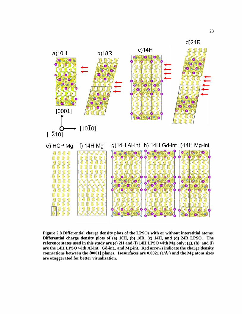
Figure 2.8 plots the isosurface of ∆𝜌 = 0021 𝐞/Å𝟑. It can be seen that in the HCP stacking
blocks, the isosurface shape is an prism (rectangular in 2 Dimension), and in the FCC stacking
region, the isosurface shape is tetragonal (triangle) [60]. The isosurface shape in pure Mg 14H
LPSO (Figure 2.8f) changes to tetragonal. It is worth noting that there are no connections between
the {0001} planes with ∆𝜌 in HCP Mg and pure Mg 14H LPSO[57]. However, the formation of
L12 cluster by solute atoms not only increases the charge density at the FCC stacking faults region,
but also connects the charge density in the HCP stacking blocks (between L12 clusters along [0001]
direction) (red arrows in Figure 2.8a, b, c, d). Such connections between the {0001] planes are
likely to result from the solute atom rich stacking faults regions. Since the denser charge density
imply the stronger bonding between atoms[57] and also Young’s modulus is proportional to
∆𝜌[60], the origin of the enhanced Young’s modulus of LPSOs comes from not only the formation
of the L12 cluster but also the connections of the {0001} planes in the HCP stacking layers.
23
Figure 2.8 Differential charge density plots of the LPSOs with or without interstitial atoms.
Differential charge density plots of (a) 10H, (b) 18R, (c) 14H, and (d) 24R LPSO. The
reference states used in this study are (e) 2H and (f) 14H LPSO with Mg only; (g), (h), and (i)
are the 14H LPSO with Al-int., Gd-int., and Mg-int. Red arrows indicate the charge density
connections between the {0001] planes. Isosurfaces are 0.0021 (e/Å 3) and the Mg atom sizes
are exaggerated for better visualization.

24
It is interesting to know how the contributions of elastic properties of the HCP layers in a
LPSO phase are changing. According to Miedema et al.[61] and Wu et al.[62], for pure alkali
metals and non-transition metals, √𝐵/𝑉𝑚 is linearly proportional to charge density at the boundary
of the Wigner-Seitz cell (𝑛𝑊𝑆), where B is the bulk modulus and 𝑉𝑚 the molar volume of the
element. This relation can be applied to the HCP stacking layers in the LPSO phases in order to
explain the partial charge to these stacking regions. Since the HCP stacking layers in the LPSO
phases are compressed along (0001) direction compared to HCP Mg structure (c.f. in Figure 2.8)
and the nearest neighbor interatomic distance of those region (3.162 Å ) is smaller than that of HCP
Mg structure (3.178 Å ), the volume of those regions is smaller than the HCP Mg structure.
Moreover, the bulk modulus of those regions should be larger than that of the HCP Mg structure
because the correlation between the bulk modulus and the nearest neighbor interatomic distance,
bulk modulus decreases owing to lattice expansion, described by Ganeshan et al.[51]. Thus, the
√𝐵/𝑉𝑚 values of the HCP stacking region in the LPSO phases are larger than the corresponding
values of HCP Mg. This means that the charge densities of the HCP stacking regions in the LPSO
are larger than that of the HCP Mg.

25
Chapter 3
First-Principles Calculations and Thermodynamic Modelling of Long
Periodic Stacking Ordered (LPSO) Phases in Mg-Al-Gd
3.1 Introduction
Among a variety of Mg alloys, the Mg-Al based alloys, such as AZ-91D and AM-50A,
have been widely used because of their excellent mechanical strength, corrosion resistance, and die
castability[63]. To further increase their strength and usage at higher temperatures, such as in
automotive powertrains above 125 oC[63], Mg alloys containing long periodic stacking ordered
(LPSO) phases[64] have received considerable attention due to their improved creep resistance and
strength[10], [12], [13], [65]. For example, it has been reported that the Mg97Zn1Y2 alloys with
various LPSO phases show outstanding creep resistance[64], [66] as well as excellent tensile yield
strength above 600 MPa and an elongation of 5% at room temperature[10], [67].
The LPSO phases observed in Mg-TM (Transition Metal)-RE (Rare Earth) ternary systems
[6], [8], [17], [19] consist of periodic ordered FCC stacking layers in the structural block (SB);
[17]–[19] see Figure 2.1. Among various LPSOs, 14H and 18R are frequently observed[6], [8],
[17]–[19]. By analyzing the crystal structures of LPSOs in the Mg-Al-Gd system, Egusa et al.[23],
Kishida et al.[6], [17], [18], and Yokobayashi et al.[8], [19] discovered the L12 type clusters in SBs
of the 14H and 18R LPSO phases in terms of the in-plane ordering of Gd and Al atoms in FCC
stacking layer regions, and Kimizuka et al.[25], [68] and Kishida et al.[17], [69] reported the
periodic formation of Gd8Al6 with a L12 type atomic arrangement is long range order.

26
Furthermore, Kishida et al.[18], [69] suggested that there might exist interstitial atoms at
the center of the L12 clusters in both Mg-Zn-Y and Mg-Al-RE systems based on scanning
transmission electron microscopy (STEM) observations. First-principle calculations based on
density functional theory (DFT) by Saal et al.[14] and Kishida et al.[18], [69] support this
suggestion. Thermodynamic stability of many LPSO phases at 0 K was investigated by Saal et
al.[14] using DFT-based first-principles calculations with the interstitial atoms at the center of the
L12 clusters considered. However, their thermodynamic stability at finite temperatures has not been
studied except in the Mg-Y-Zn[70], [71] and Mg-Gd-Zn[72] systems, where the 14H and 18R
LPSO phases were treated as stoichiometric compounds of Mg12ZnRE and Mg10ZnRE, respectively.
In the present work, the thermodynamic properties of the 10H, 14H, 18R and 24R LPSO
phases in the Mg-Al-Gd ternary system are modeled by means of the CALPHAD (calculation of
phase diagram) method[73]. The L12 clusters and the existence of interstitial atoms within their
center are considered in terms of the compound energy formalism (CEF)[74]. DFT-based first-
principles calculations are performed to provide thermodynamic properties at finite-temperatures
[75] for CALPHAD modeling.
3.2 First-Principles Calculations
The space groups of 10H and 14H LPSO phases used in the present work are Cmce and
P63/mcm, respectively, while the space group of 18R and 24R LPSO phases are C2/m [6], [18].
Crystal structures of 10H, 18R, 14H, and 24R LPSO phases are shown in Figure 2.1a-d,
respectively, and the L12 cluster with an interstitial atom is depicted in Figure 2.1f. The lattice of
the LPSO phases can be divided into four sublattices based on their Wyckoff positions as follows
[17]–[19]
Equation 3.1 (𝑴𝒈)𝟔𝟖+𝟐𝟒𝒙(𝑴𝒈,𝑮𝒅, 𝑨𝒍)𝟏𝟔(𝑴𝒈,𝑮𝒅,𝑨𝒍)𝟏𝟐(𝑴𝒈,𝑮𝒅, 𝑨𝒍, 𝑽𝒂)𝟐

27
where x=1, 2, 3, and 4 for 10H, 18R, 14H, and 24R LPSO phases, respectively. The 1st sublattice
(sublattice Ⅰ) represents the layers outside of the L12 cluster which consists of mostly Mg atoms
located in the HCP and FCC lattices, the 2nd sublattice (sublattice Ⅱ) the corner positions of the L12
cluster, the 3rd sublattice (sublattice Ⅲ) the face-centered positions of the L12 cluster, and the 4th
sublattice (sublattice Ⅳ) the interstitial octahedral site of the L12 cluster. The supercells of the
10H, 14H, 18R and 24R LPSO phases contain 244 or 240, 170 or 168, 146 or 144, and 194 or 192
atoms with or without the interstitial atoms in the L12 cluster, respectively[18], [23]. As it can be
seen in the sublattice model above, the mixture of all elements is considered in the sublattices Ⅱ,
Ⅲ and Ⅳ.
Each endmember in CEF is defined by the sublattice model shown in Eq. 1 with only one
element in each sublattice. For mixing in sublattices Ⅱ and Ⅲ, the dilute solutions are considered
by substituting one atom in the sublattice of the supercells. The enthalpies of mixing in dilute
solutions in the sublattice Ⅳ with a supercell twice the size of the LPSO supercells are calculated
to be very small about 10 J/mole-atom. This is due to the large distance between interstitial atoms,
about six-times than that between Mg atoms, indicating ideal mixing in the sublattice.
First-principles calculations are performed using the Vienna Ab-initio Simulation Package
(VASP)[27], [28], [31]. Electron-ion interactions are described by the projector augmented-wave
(PAW) method[29], and the exchange-correlation energy functional is depicted by the generalized
gradient approximation (GGA) as implemented by Perdew, Burke, and Ernzerhof (PBE)[30]. The
f-electrons of Gd are treated as core electrons (so-called “frozen” potential), an approximation that
has shown to produce accurate thermodynamic properties for lanthanide compounds[32]–[35].
Plane wave cutoff energy of 350 eV is used for all calculations, which is at least 1.3 times higher
than the recommended values by VASP[31]. For HCP Mg with 2 atoms in the unit cell, the 29 ×
29 × 16 k-point grids are employed. The k-point meshes of 3 × 5 × 2 (10H LPSO), 6 × 6 × 2 (14H
LPSO), 6 × 3 × 3 (18R LPSO), and 3 × 2 × 2 (24R LPSO) are used for the LPSO phases. These k-

28
point meshes guarantee errors below 0.1 meV/atom (0.2 meV/atom for 24R LPSO). These
structures are fully relaxed by the Methfessel-Paxton method.[76] After relaxations, a final static
calculation using the tetrahedral method with Blöch corrections[36] is applied to predict accurate
total energy.
The Helmholtz energy, 𝐹(𝑉, 𝑇), of the present structures of interest is evaluated in terms
of the quasi-harmonic approach as a function of volume (V) and temperature (T) [75], [77]:
Equation 3.2 𝑭(𝑽, 𝑻) = 𝑬𝟎𝑲(𝑽) + 𝑭𝒗𝒊𝒃(𝑽, 𝑻) + 𝑭𝒆𝒍(𝑽, 𝑻)
where E0K(V) is the static contribution at 0 K without the zero-point vibrational energy. Fvib(V, T)
and Fel(V, T) represent the vibrational and thermal-electronic contributions to the Helmholtz
energy, respectively. To estimate E0K(V), a four-parameter Birch–Murnaghan (BM4) equation of
state (EOS),[75], [78] is used to fit the energy versus volume (E-V) data points from first-principles
calculations,
Equation 3.3 𝑬(𝑽) = 𝑨𝟏 + 𝑨𝟐𝑽−𝟐
𝟑 + 𝑨𝟑𝑽−𝟒
𝟑 +𝑨𝟒𝑽−𝟐
where A1, A2, A3 and A4 are fitting parameters. The E-V data points used in the EOS fitting are
relaxed with respect to ionic positions and cell shape at the given volumes, and nine E-V data points
are usually used. Note that the Helmholtz energy is equated to the Gibbs energy due to the zero (or
ambient) external pressure used in the present work. The thermal electronic contribution to the
Helmholtz energy is estimated based on the electronic density of states (DOS) in terms of the
Fermi–Dirac statistics for metallic systems[75].
The quasi-harmonic vibrational contributions can be obtained through phonon or the Debye
model. In calculations of phonon, the vibrational contribution to the Helmholtz energy can be
expressed as
Equation 3.4 𝑭𝒗𝒊𝒃(𝑽, 𝑻) = 𝒌𝑩𝑻∫ 𝐥𝐧 [𝟐 𝐬𝐢𝐧𝐡ℏ𝝎
𝟐𝒌𝑩𝑻]
∞
𝟎𝒈(𝝎,𝑽)𝒅𝝎
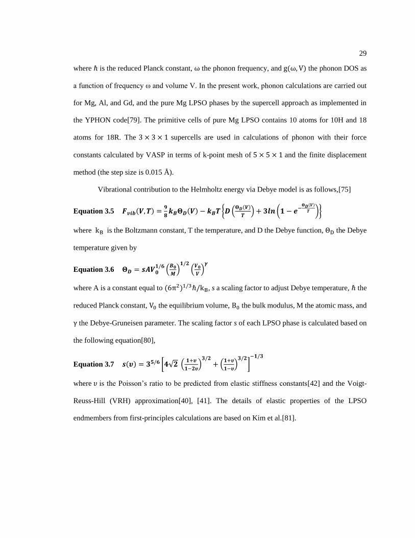
29
where ℏ is the reduced Planck constant, ω the phonon frequency, and g(ω, V) the phonon DOS as
a function of frequency ω and volume V. In the present work, phonon calculations are carried out
for Mg, Al, and Gd, and the pure Mg LPSO phases by the supercell approach as implemented in
the YPHON code[79]. The primitive cells of pure Mg LPSO contains 10 atoms for 10H and 18
atoms for 18R. The 3 × 3 × 1 supercells are used in calculations of phonon with their force
constants calculated by VASP in terms of k-point mesh of 5 × 5 × 1 and the finite displacement
method (the step size is 0.015 Å ).
Vibrational contribution to the Helmholtz energy via Debye model is as follows,[75]
Equation 3.5 𝑭𝒗𝒊𝒃(𝑽, 𝑻) =𝟗
𝟖𝒌𝑩𝚯𝑫(𝑽) − 𝒌𝑩𝑻 {𝑫(
𝚯𝑫(𝑽)
𝑻) + 𝟑𝒍𝒏(𝟏 − 𝒆−
𝚯𝑫(𝑽)
𝑻 )}
where kB is the Boltzmann constant, T the temperature, and D the Debye function, ΘD the Debye
temperature given by
Equation 3.6 𝚯𝑫 = 𝒔𝑨𝑽𝟎𝟏/𝟔(𝑩𝟎
𝑴)𝟏/𝟐(𝑽𝟎
𝑽)𝜸
where A is a constant equal to (6π2)1/3ℏ/kB, s a scaling factor to adjust Debye temperature, ℏ the
reduced Planck constant, V0 the equilibrium volume, B0 the bulk modulus, M the atomic mass, and
γ the Debye-Gruneisen parameter. The scaling factor s of each LPSO phase is calculated based on
the following equation[80],
Equation 3.7 𝒔(𝝊) = 𝟑𝟓/𝟔 [𝟒√𝟐 (𝟏+𝝊
𝟏−𝟐𝝊)𝟑/𝟐+ (
𝟏+𝝊
𝟏−𝝊)𝟑/𝟐]−𝟏/𝟑
where 𝜐 is the Poisson’s ratio to be predicted from elastic stiffness constants[42] and the Voigt-
Reuss-Hill (VRH) approximation[40], [41]. The details of elastic properties of the LPSO
endmembers from first-principles calculations are based on Kim et al.[81].
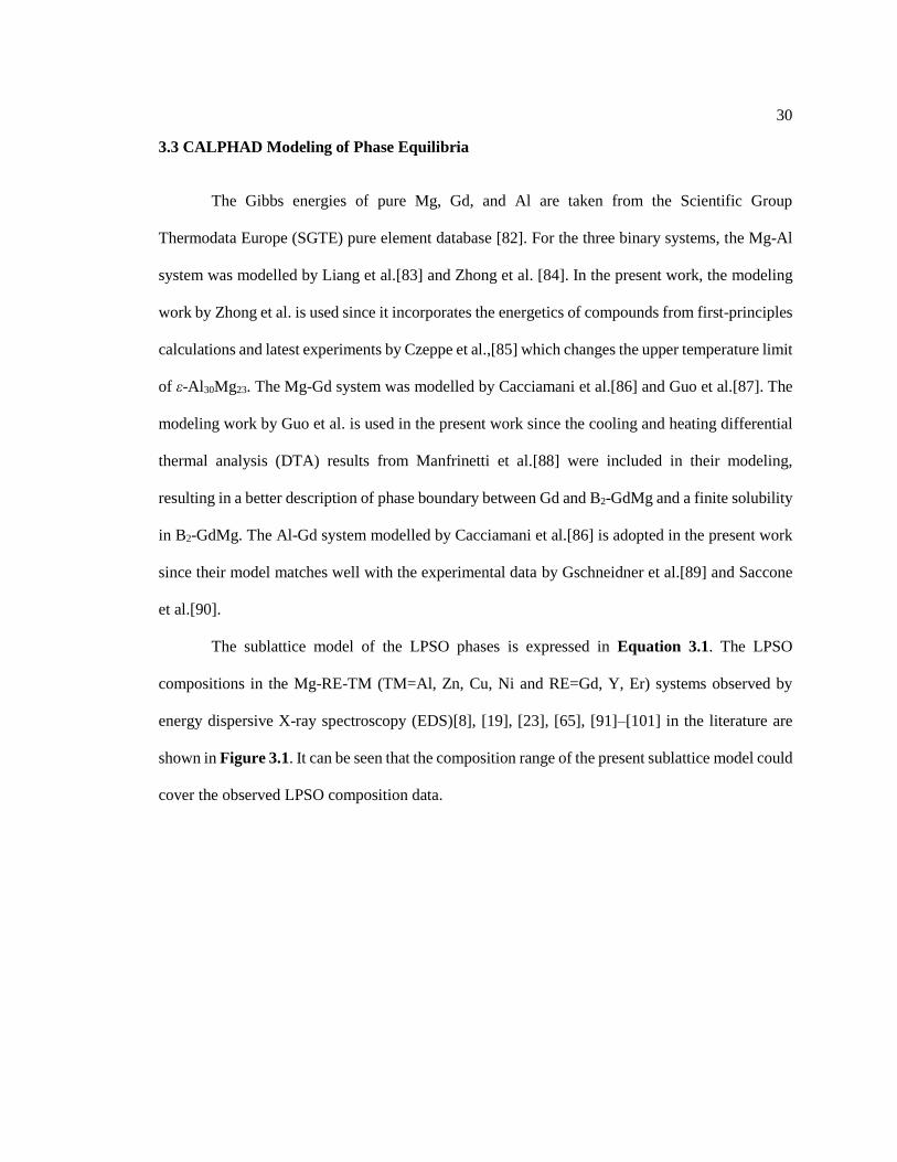
30
3.3 CALPHAD Modeling of Phase Equilibria
The Gibbs energies of pure Mg, Gd, and Al are taken from the Scientific Group
Thermodata Europe (SGTE) pure element database [82]. For the three binary systems, the Mg-Al
system was modelled by Liang et al.[83] and Zhong et al. [84]. In the present work, the modeling
work by Zhong et al. is used since it incorporates the energetics of compounds from first-principles
calculations and latest experiments by Czeppe et al.,[85] which changes the upper temperature limit
of ε-Al30Mg23. The Mg-Gd system was modelled by Cacciamani et al.[86] and Guo et al.[87]. The
modeling work by Guo et al. is used in the present work since the cooling and heating differential
thermal analysis (DTA) results from Manfrinetti et al.[88] were included in their modeling,
resulting in a better description of phase boundary between Gd and B2-GdMg and a finite solubility
in B2-GdMg. The Al-Gd system modelled by Cacciamani et al.[86] is adopted in the present work
since their model matches well with the experimental data by Gschneidner et al.[89] and Saccone
et al.[90].
The sublattice model of the LPSO phases is expressed in Equation 3.1. The LPSO
compositions in the Mg-RE-TM (TM=Al, Zn, Cu, Ni and RE=Gd, Y, Er) systems observed by
energy dispersive X-ray spectroscopy (EDS)[8], [19], [23], [65], [91]–[101] in the literature are
shown in Figure 3.1. It can be seen that the composition range of the present sublattice model could
cover the observed LPSO composition data.
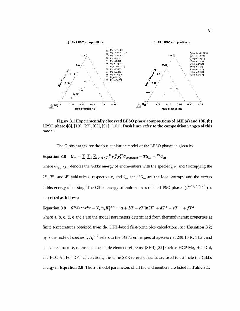
31
Figure 3.1 Experimentally observed LPSO phase compositions of 14H (a) and 18R (b)
LPSO phases[8], [19], [23], [65], [91]–[101]. Dash lines refer to the composition ranges of this
model.
The Gibbs energy for the four-sublattice model of the LPSO phases is given by
Equation 3.8 𝑮𝒎 = ∑ ∑ ∑ 𝒚𝑴𝒈Ⅰ 𝒚𝒋
Ⅱ𝒚𝒌Ⅲ𝒚𝒍
Ⅳ𝑮𝑴𝒈:𝒋:𝒌:𝒍𝒍𝒌𝒋 − 𝑻𝑺𝒎 + 𝑮𝒎𝒙𝒔
where 𝐺𝑀𝑔:𝑗:𝑘:𝑙 denotes the Gibbs energy of endmembers with the species j, k, and l occupying the
2nd, 3rd, and 4th sublattices, respectively, and 𝑆𝑚 and 𝐺𝑚𝑥𝑠 are the ideal entropy and the excess
Gibbs energy of mixing. The Gibbs energy of endmembers of the LPSO phases (𝐺𝑀𝑔𝑝𝐺𝑑𝑞𝐴𝑙𝑟) is
described as follows:
Equation 3.9 𝑮𝑴𝒈𝒑𝑮𝒅𝒒𝑨𝒍𝒓 − ∑ 𝒏𝒊𝑯𝒊𝑺𝑬𝑹
𝒊 = 𝒂 + 𝒃𝑻 + 𝒄𝑻 𝐥𝐧(𝑻) + 𝒅𝑻𝟐 + 𝒆𝑻−𝟏 + 𝒇𝑻𝟑
where a, b, c, d, e and f are the model parameters determined from thermodynamic properties at
finite temperatures obtained from the DFT-based first-principles calculations, see Equation 3.2;
𝑛𝑖 is the mole of species 𝑖; 𝐻𝑖𝑆𝐸𝑅 refers to the SGTE enthalpies of species 𝑖 at 298.15 K, 1 bar, and
its stable structure, referred as the stable element reference (SER),[82] such as HCP Mg, HCP Gd,
and FCC Al. For DFT calculations, the same SER reference states are used to estimate the Gibbs
energy in Equation 3.9. The a-f model parameters of all the endmembers are listed in Table 3.1.
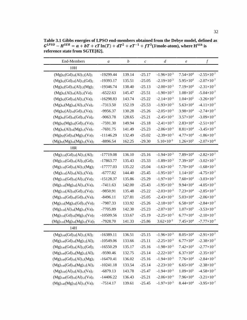
32
Table 3.1 Gibbs energies of LPSO end-members obtained from the Debye model, defined as
𝑮𝑳𝑷𝑺𝑶 −𝑯𝑺𝑬𝑹 = 𝒂 + 𝒃𝑻 + 𝒄𝑻 𝐥𝐧(𝑻) + 𝒅𝑻𝟐 + 𝒆𝑻−𝟏 + 𝒇𝑻𝟑(J/mole-atom), where HSER is
reference state from SGTE[82].
End-Members a b c d e f
10H
(Mg)92(Gd)16(Al)12(Al)2 -19299.44 139.14 -25.17 -1.96×10⁻³ 7.54×10⁴ -2.55×10⁻⁷
(Mg)92(Gd)16(Al)12(Gd)2 -19393.17 135.51 -25.05 -2.19×10⁻³ 5.95×10⁴ -2.07×10⁻⁷
(Mg)92(Gd)16(Al)12(Mg)2 -19346.74 138.40 -25.13 -2.00×10⁻³ 7.19×10⁴ -2.31×10⁻⁷
(Mg)92(Al)16(Al)12(Va)2 -6522.63 145.47 -25.51 -1.90×10⁻³ 1.08×10⁵ -5.04×10⁻⁷
(Mg)92(Gd)16(Al)12(Va)2 -16298.83 143.74 -25.22 -2.14×10⁻³ 1.04×10⁵ -3.26×10⁻⁷
(Mg)92(Mg)16(Al)12(Va)2 -7313.50 152.19 -25.53 -1.93×10⁻³ 5.63×10⁴ -4.11×10⁻⁷
(Mg)92(Al)16(Gd)12(Va)2 -9956.37 130.28 -25.26 -2.05×10⁻³ 3.98×10⁴ -2.74×10⁻⁷
(Mg)92(Gd)16(Gd)12(Va)2 -9063.78 128.65 -25.21 -2.45×10⁻³ 3.57×10⁴ -3.09×10⁻⁷
(Mg)92(Mg)16(Gd)12(Va)2 -7591.30 149.94 -25.18 -2.41×10⁻³ 2.83×10⁴ -2.51×10⁻⁷
(Mg)92(Al)16(Mg)12(Va)2 -7691.75 141.49 -25.23 -2.06×10⁻³ 8.81×10⁴ -3.45×10⁻⁷
(Mg)92(Gd)16(Mg)12(Va)2 -11146.29 132.49 -25.02 -2.39×10⁻³ 4.77×10⁴ -1.86×10⁻⁷
(Mg)92(Mg)16(Mg)12(Va)2 -8896.54 162.25 -29.30 5.10×10⁻³ 1.26×10⁵ -2.07×10⁻⁶
18R
(Mg)116(Gd)16(Al)12(Al)2 -17719.08 136.10 -25.16 -1.94×10⁻³ 7.89×10⁴ -2.82×10⁻⁷
(Mg)116(Gd)16(Al)12(Gd)2 -17863.77 135.43 -25.33 -1.89×10⁻³ 7.39×10⁴ -3.02×10⁻⁷
(Mg)116(Gd)16(Al)12(Mg)2 -17777.03 135.22 -25.04 -1.63×10⁻³ 7.70×10⁴ -1.68×10⁻⁷
(Mg)116(Al)16(Al)12(Va)2 -6777.82 144.40 -25.45 -1.95×10⁻³ 1.14×10⁵ -4.75×10⁻⁷
(Mg)116(Gd)16(Al)12(Va)2 -15128.37 135.86 -25.29 -1.97×10⁻³ 7.60×10⁴ -3.03×10⁻⁷
(Mg)116(Mg)16(Al)12(Va)2 -7411.63 142.00 -25.43 -1.95×10⁻³ 9.94×10⁴ -4.05×10⁻⁷
(Mg)116(Al)16(Gd)12(Va)2 -9850.91 135.48 -25.22 -2.03×10⁻³ 7.23×10⁴ -2.85×10⁻⁷
(Mg)116(Gd)16(Gd)12(Va)2 -8496.11 127.81 -25.05 -2.43×10⁻³ 5.03×10⁴ -2.06×10⁻⁷
(Mg)116(Mg)16(Gd)12(Va)2 -7987.33 133.92 -25.26 -2.18×10⁻³ 6.58×10⁴ -2.84×10⁻⁷
(Mg)116(Al)16(Mg)12(Va)2 -7705.89 142.30 -25.23 -2.07×10⁻³ 1.07×10⁵ -3.53×10⁻⁷
(Mg)116(Gd)16(Mg)12(Va)2 -10509.56 133.67 -25.19 -2.25×10⁻³ 6.77×10⁴ -2.10×10⁻⁷
(Mg)116(Mg)16(Mg)12(Va)2 -7928.70 141.33 -25.86 3.62×10⁻³ 7.45×10⁴ -7.77×10⁻⁷
14H
(Mg)140(Gd)16(Al)12(Al)2 -16389.11 136.51 -25.15 -1.96×10⁻³ 8.05×10⁴ -2.91×10⁻⁷
(Mg)140(Gd)16(Mg)12(Al)2 -10549.06 133.66 -25.11 -2.25×10⁻³ 6.77×10⁴ -2.38×10⁻⁷
(Mg)140(Gd)16(Al)12(Gd)2 -16550.29 135.17 -25.16 -1.98×10⁻³ 7.42×10⁴ -2.77×10⁻⁷
(Mg)140(Gd)16(Mg)12(Al)2 -9590.46 132.75 -25.14 -2.22×10⁻³ 6.37×10⁴ -2.35×10⁻⁷
(Mg)140(Gd)16(Al)12(Mg)2 -16470.41 136.02 -25.16 -1.94×10⁻³ 7.76×10⁴ -2.84×10⁻⁷
(Mg)140(Gd)16(Mg)12(Al)2 -10241.18 133.54 -25.14 -2.23×10⁻³ 6.65×10⁴ -2.38×10⁻⁷
(Mg)140(Al)16(Al)12(Va)2 -6879.13 143.78 -25.47 -1.94×10⁻³ 1.09×10⁵ -4.58×10⁻⁷
(Mg)140(Gd)16(Al)12(Va)2 -14406.22 136.43 -25.21 -2.06×10⁻³ 7.96×10⁴ -3.21×10⁻⁷
(Mg)140(Mg)16(Al)12(Va)2 -7514.17 139.61 -25.45 -1.97×10⁻³ 8.44×10⁴ -3.95×10⁻⁷
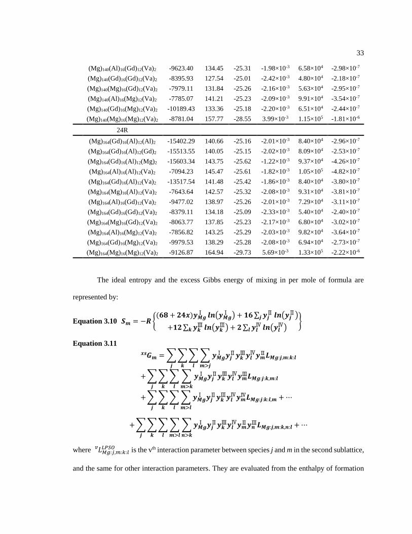
33
(Mg)140(Al)16(Gd)12(Va)2 -9623.40 134.45 -25.31 -1.98×10⁻³ 6.58×10⁴ -2.98×10⁻⁷
(Mg)140(Gd)16(Gd)12(Va)2 -8395.93 127.54 -25.01 -2.42×10⁻³ 4.80×10⁴ -2.18×10⁻⁷
(Mg)140(Mg)16(Gd)12(Va)2 -7979.11 131.84 -25.26 -2.16×10⁻³ 5.63×10⁴ -2.95×10⁻⁷
(Mg)140(Al)16(Mg)12(Va)2 -7785.07 141.21 -25.23 -2.09×10⁻³ 9.91×10⁴ -3.54×10⁻⁷
(Mg)140(Gd)16(Mg)12(Va)2 -10189.43 133.36 -25.18 -2.20×10⁻³ 6.51×10⁴ -2.44×10⁻⁷
(Mg)140(Mg)16(Mg)12(Va)2 -8781.04 157.77 -28.55 3.99×10⁻³ 1.15×10⁵ -1.81×10⁻⁶
24R
(Mg)164(Gd)16(Al)12(Al)2 -15402.29 140.66 -25.16 -2.01×10⁻³ 8.40×10⁴ -2.96×10⁻⁷
(Mg)164(Gd)16(Al)12(Gd)2 -15513.55 140.05 -25.15 -2.02×10⁻³ 8.09×10⁴ -2.53×10⁻⁷
(Mg)164(Gd)16(Al)12(Mg)2 -15603.34 143.75 -25.62 -1.22×10⁻³ 9.37×10⁴ -4.26×10⁻⁷
(Mg)164(Al)16(Al)12(Va)2 -7094.23 145.47 -25.61 -1.82×10⁻³ 1.05×10⁵ -4.82×10⁻⁷
(Mg)164(Gd)16(Al)12(Va)2 -13517.54 141.48 -25.42 -1.86×10⁻³ 8.40×10⁴ -3.80×10⁻⁷
(Mg)164(Mg)16(Al)12(Va)2 -7643.64 142.57 -25.32 -2.08×10⁻³ 9.31×10⁴ -3.81×10⁻⁷
(Mg)164(Al)16(Gd)12(Va)2 -9477.02 138.97 -25.26 -2.01×10⁻³ 7.29×10⁴ -3.11×10⁻⁷
(Mg)164(Gd)16(Gd)12(Va)2 -8379.11 134.18 -25.09 -2.33×10⁻³ 5.40×10⁴ -2.40×10⁻⁷
(Mg)164(Mg)16(Gd)12(Va)2 -8063.77 137.85 -25.23 -2.17×10⁻³ 6.80×10⁴ -3.02×10⁻⁷
(Mg)164(Al)16(Mg)12(Va)2 -7856.82 143.25 -25.29 -2.03×10⁻³ 9.82×10⁴ -3.64×10⁻⁷
(Mg)164(Gd)16(Mg)12(Va)2 -9979.53 138.29 -25.28 -2.08×10⁻³ 6.94×10⁴ -2.73×10⁻⁷
(Mg)164(Mg)16(Mg)12(Va)2 -9126.87 164.94 -29.73 5.69×10⁻³ 1.33×10⁵ -2.22×10⁻⁶
The ideal entropy and the excess Gibbs energy of mixing in per mole of formula are
represented by:
Equation 3.10 𝑺𝒎 = −𝑹{(𝟔𝟖 + 𝟐𝟒𝒙)𝒚𝑴𝒈
Ⅰ 𝒍𝒏(𝒚𝑴𝒈Ⅰ ) + 𝟏𝟔∑ 𝒚𝒋
Ⅱ 𝒍𝒏(𝒚𝒋Ⅱ)𝒋
+𝟏𝟐∑ 𝒚𝒌Ⅲ 𝒍𝒏(𝒚𝒌
Ⅲ)𝒌 + 𝟐∑ 𝒚𝒍Ⅳ 𝒍𝒏(𝒚𝒍
Ⅳ)𝒍
}
Equation 3.11
𝑮𝒎 𝒙𝒔 =∑∑∑∑𝒚𝑴𝒈
Ⅰ 𝒚𝒋Ⅱ𝒚𝒌
Ⅲ𝒚𝒍Ⅳ𝒚𝒎
Ⅱ𝑳𝑴𝒈:𝒋,𝒎:𝒌:𝒍𝒎>𝒋𝒍𝒌𝒋
+∑∑∑∑ 𝒚𝑴𝒈Ⅰ 𝒚𝒋
Ⅱ𝒚𝒌Ⅲ𝒚𝒍
Ⅳ𝒚𝒎Ⅲ𝑳𝑴𝒈:𝒋:𝒌,𝒎:𝒍
𝒎>𝒌𝒍𝒌𝒋
+∑∑∑∑𝒚𝑴𝒈Ⅰ 𝒚𝒋
Ⅱ𝒚𝒌Ⅲ𝒚𝒍
Ⅳ𝒚𝒎Ⅳ𝑳𝑴𝒈:𝒋:𝒌:𝒍,𝒎
𝒎>𝒍𝒍𝒌𝒋
+⋯
+∑∑∑∑∑𝒚𝑴𝒈Ⅰ 𝒚𝒋
Ⅱ𝒚𝒌Ⅲ𝒚𝒍
Ⅳ𝒚𝒎Ⅱ𝒚𝒏
Ⅲ𝑳𝑴𝒈:𝒋,𝒎:𝒌,𝒏:𝒍𝒏>𝒌𝒎>𝒍𝒍𝒌𝒋
+⋯
where 𝐿𝑀𝑔:𝑗,𝑚:𝑘:𝑙𝐿𝑃𝑆𝑂𝑣 is the vth interaction parameter between species j and m in the second sublattice,
and the same for other interaction parameters. They are evaluated from the enthalpy of formation

34
from DFT-based first-principles calculations. 𝐿𝑀𝑔:𝑗,𝑚:𝑘:𝑙𝐿𝑃𝑆𝑂𝑣 of all the endmembers are listed in
Table 3.2.
Table 3.2 Interaction parameters in individual sublattices (kJ/mol-atom).
LPSO 10H 18R 14H 24R
i,j Al-
Gd
Al-
Mg
Gd-
Mg
Al-
Gd
Al-
Mg
Gd-
Mg
Al-
Gd
Al-
Mg
Gd-
Mg
Al-
Gd
Al-
Mg
Gd-
Mg
𝐿Mg:i,j:Al:Va𝐿𝑃𝑆𝑂0 -1.139 -0.018 1.287 -1.127 0.217 -1.757 0.733 1.259 -2.037 5.767 -0.096 -5.577
𝐿Mg:i,j:Al:Va𝐿𝑃𝑆𝑂1 5.594 0.928 1.598 5.214 0.081 4.240 4.491 -0.423 3.473 -1.642 -6.829 -3.572
𝐿Mg:i,j:Gd:Va𝐿𝑃𝑆𝑂0 -0.409 0.471 1.435 -2.160 -0.585 0.961 0.162 0.248 -0.078 0.845 0.363 -0.617
𝐿Mg:i,j:Gd:Va𝐿𝑃𝑆𝑂1 2.162 0.102 0.679 3.073 -0.147 1.094 1.194 -0.272 0.337 -6.257 -7.507 -6.422
𝐿Mg:i,j:Mg:Va𝐿𝑃𝑆𝑂0 -0.574 -0.253 -0.842 -1.709 0.210 0.811 -0.992 -0.081 0.189 3.060 -0.825 -3.837
𝐿Mg:i,j:Mg:Va𝐿𝑃𝑆𝑂1 5.454 0.345 2.032 3.504 0.354 1.142 2.819 0.118 0.848 -1.948 -7.166 -3.960
𝐿Mg:Al:i,j:Va𝐿𝑃𝑆𝑂0 -0.202 -0.024 0.297 0.061 0.098 0.194 0.717 0.597 0.204 -3.863 -3.009 1.738
𝐿Mg:Al:i,j:Va𝐿𝑃𝑆𝑂1 -7.607 0.057 -3.640 -5.992 -0.126 -3.025 -5.938 -0.691 -2.680 -7.611 -2.409 -8.004
𝐿Mg:Gd:i,j:Va𝐿𝑃𝑆𝑂0 9.128 7.159 -1.364 5.889 4.652 -1.627 4.977 3.702 -1.393 1.436 1.102 -0.593
𝐿Mg:Gd:i,j:Va𝐿𝑃𝑆𝑂1 -5.591 -6.042 0.697 -3.321 -3.987 0.066 -3.032 -3.218 -0.037 -3.028 -2.808 -2.552
𝐿Mg:Mg:i,j:Va𝐿𝑃𝑆𝑂0 0.655 -0.119 -0.629 0.484 -0.043 0.021 0.557 -0.034 -0.135 0.187 -0.435 -0.312
𝐿Mg:Mg:i,j:Va𝐿𝑃𝑆𝑂1 -5.223 -0.389 -1.509 -4.607 -0.204 -1.210 -4.042 -0.392 -0.977 -6.875 -5.013 -5.545
3.4 Results and Discussion
To benchmark the reliability of first-principles calculations for the Mg-Al-Gd system,
lattice parameters of pure elements are calculated and compared to experimental and calculated
data available in the literature in Table 3.3 [102]–[104]. As can be seen in the table, the lattice
parameters of Mg, Al, and Gd are in good agreement with the corresponding experimental results.
The relative errors between calculated and experimental lattice parameters of these pure elements
are less than 1%. Figure 3.2 shows the phonon results of HCP Mg and pure Mg LPSO endmembers,
(Mg)68+24x(Mg)16(Mg)12(Va)2, and the phonon dispersion curves of HCP Mg (Figure 3.2a) are
calculated at its equilibrium volume, comparing favorably with experiments[105]. The phonon
DOS curves between HCP Mg and the Mg LPSO endmembers are plotted in Figure 3.2b. All the
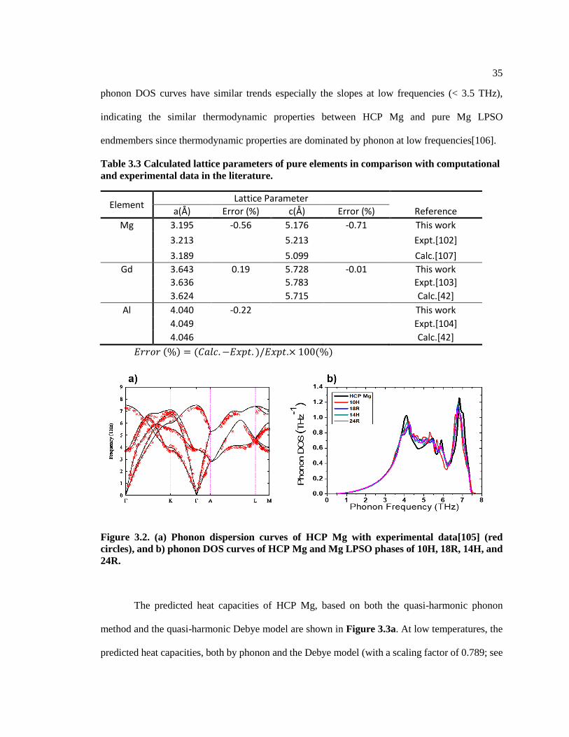
35
phonon DOS curves have similar trends especially the slopes at low frequencies (< 3.5 THz),
indicating the similar thermodynamic properties between HCP Mg and pure Mg LPSO
endmembers since thermodynamic properties are dominated by phonon at low frequencies[106].
Table 3.3 Calculated lattice parameters of pure elements in comparison with computational
and experimental data in the literature.
Element Lattice Parameter
a(Å) Error (%) c(Å) Error (%) Reference Mg 3.195 -0.56 5.176 -0.71 This work
3.213 5.213 Expt.[102] 3.189 5.099 Calc.[107]
Gd 3.643 0.19 5.728 -0.01 This work 3.636 5.783 Expt.[103] 3.624 5.715 Calc.[42]
Al 4.040 -0.22 This work 4.049 Expt.[104] 4.046 Calc.[42]
𝐸𝑟𝑟𝑜𝑟 (%) = (𝐶𝑎𝑙𝑐. −𝐸𝑥𝑝𝑡. )/𝐸𝑥𝑝𝑡.× 100(%)
Figure 3.2. (a) Phonon dispersion curves of HCP Mg with experimental data[105] (red
circles), and b) phonon DOS curves of HCP Mg and Mg LPSO phases of 10H, 18R, 14H, and
24R.
The predicted heat capacities of HCP Mg, based on both the quasi-harmonic phonon
method and the quasi-harmonic Debye model are shown in Figure 3.3a. At low temperatures, the
predicted heat capacities, both by phonon and the Debye model (with a scaling factor of 0.789; see
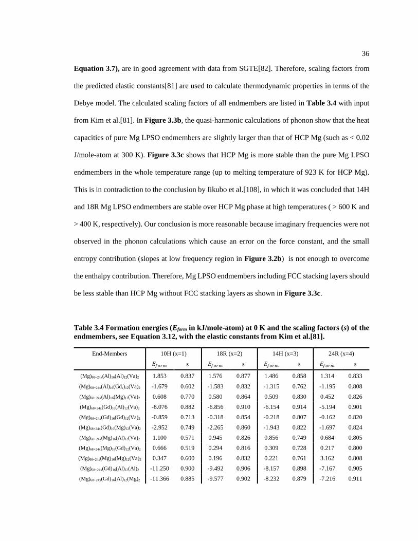
36
Equation 3.7), are in good agreement with data from SGTE[82]. Therefore, scaling factors from
the predicted elastic constants[81] are used to calculate thermodynamic properties in terms of the
Debye model. The calculated scaling factors of all endmembers are listed in Table 3.4 with input
from Kim et al.[81]. In Figure 3.3b, the quasi-harmonic calculations of phonon show that the heat
capacities of pure Mg LPSO endmembers are slightly larger than that of HCP Mg (such as < 0.02
J/mole-atom at 300 K). Figure 3.3c shows that HCP Mg is more stable than the pure Mg LPSO
endmembers in the whole temperature range (up to melting temperature of 923 K for HCP Mg).
This is in contradiction to the conclusion by Iikubo et al.[108], in which it was concluded that 14H
and 18R Mg LPSO endmembers are stable over HCP Mg phase at high temperatures ( > 600 K and
> 400 K, respectively). Our conclusion is more reasonable because imaginary frequencies were not
observed in the phonon calculations which cause an error on the force constant, and the small
entropy contribution (slopes at low frequency region in Figure 3.2b) is not enough to overcome
the enthalpy contribution. Therefore, Mg LPSO endmembers including FCC stacking layers should
be less stable than HCP Mg without FCC stacking layers as shown in Figure 3.3c.
Table 3.4 Formation energies (Eform in kJ/mole-atom) at 0 K and the scaling factors (s) of the
endmembers, see Equation 3.12, with the elastic constants from Kim et al.[81].
End-Members 10H (x=1) 18R (x=2) 14H (x=3) 24R (x=4)
𝐸𝑓𝑜𝑟𝑚 s 𝐸𝑓𝑜𝑟𝑚 s 𝐸𝑓𝑜𝑟𝑚 s 𝐸𝑓𝑜𝑟𝑚 s
(Mg)68+24x(Al)16(Al)12(Va)2 1.853 0.837 1.576 0.877 1.486 0.858 1.314 0.833
(Mg)68+24x(Al)16(Gd,)12(Va)2 -1.679 0.602 -1.583 0.832 -1.315 0.762 -1.195 0.808
(Mg)68+24x(Al)16(Mg)12(Va)2 0.608 0.770 0.580 0.864 0.509 0.830 0.452 0.826
(Mg)68+24x(Gd)16(Al)12(Va)2 -8.076 0.882 -6.856 0.910 -6.154 0.914 -5.194 0.901
(Mg)68+24x(Gd)16(Gd)12(Va)2 -0.859 0.713 -0.318 0.854 -0.218 0.807 -0.162 0.820
(Mg)68+24x(Gd)16(Mg)12(Va)2 -2.952 0.749 -2.265 0.860 -1.943 0.822 -1.697 0.824
(Mg)68+24x(Mg)16(Al)12(Va)2 1.100 0.571 0.945 0.826 0.856 0.749 0.684 0.805
(Mg)68+24x(Mg)16(Gd)12(Va)2 0.666 0.519 0.294 0.816 0.309 0.728 0.217 0.800
(Mg)68+24x(Mg)16(Mg)12(Va)2 0.347 0.600 0.196 0.832 0.221 0.761 3.162 0.808
(Mg)68+24x(Gd)16(Al)12(Al)2 -11.250 0.900 -9.492 0.906 -8.157 0.898 -7.167 0.905
(Mg)68+24x(Gd)16(Al)12(Mg)2 -11.366 0.885 -9.577 0.902 -8.232 0.879 -7.216 0.911

37
(Mg)68+24x(Gd)16(Al)12(Gd)2 -11.385 0.849 -9.582 0.842 -8.316 0.876 -7.275 0.900
Figure 3.3 Comparison of (a) heat capacity of HCP Mg with experimental data from
SGTE[82], (b) heat capacities of Mg-only LPSO phases, and (c) Gibbs energy differences of
various pure Mg LPSO phases with respect to HCP Mg.

38
Calculated formation energies of all LPSO endmembers at 0 K with pure element reference
states are obtained from Equation 3.12 and summarized in Table 3.4 and Figure 3.4.
Equation 3.12 𝑬𝒇𝒐𝒓𝒎(𝑳𝑷𝑺𝑶) = 𝑬(𝑳𝑷𝑺𝑶) − 𝟏
𝑵∑ 𝑵𝒊𝑬𝒊𝒊
where Ei is the total energy of stable bulk state of species per atom of species i, and Ni the moles
of species i. The calculated formation energies at 0 K are in good agreement with the results by
Saal et al.[14]. To illustrate the energetics for atomic occupancy at the interstitial site in the L12
cluster, the formation energies of endmembers with and without interstitial elements are plotted in
Figure 3.5. It can be seen in Figure 3.5b that the formation energy of GdIIAlIIIVaIV, i.e., with the
interstitial site being vacant, is substantially higher than the surfaces of the formation energy
bounded by GdIIAlIII(Al or Gd or Mg)IV, i.e. with the interstitial site occupied. This signifies that
the interstitial sites are energetically favored with atoms and confirms the conclusions by Kishida
et al.[18], [69]. The parameters in Gibbs energy functions of all endmembers, see Equation 3.9,
and sublattice interaction parameters, see Equation 3.11, are evaluated and listed in Table 3.1 and
Table 3.2, also in Appendix B. It can be seen that the interaction parameters in the interstitial
sublattice, i.e., sublattice IV, is rather small, indicating the near ideal mixing in the sublattice due
probably to their very small compositional variation.

39
5 6 7 8
-12
-10
-8
-6
-4
-2
0
2
24R14H18R
GdIIAl
IIIVa
IV
GdIIAl
IIIAl
IV
GdIIAl
IIIMg
IV
GdIIAl
IIIGd
IV
AlIIAl
IIIVa
IV
AlIIGd
IIIVa
IV
AlIIMg
IIIVa
IV
GdIIGd
IIIVa
IV
GdIIMg
IIIVa
IV
MgIIAl
IIIVa
IV
MgIIGd
IIIVa
IV
MgIIMg
IIIVa
IV
GdIIAl
IIIMg
IV-Saal
Form
ation
Energ
y (
kJ/m
ol-
ato
m)
Number of layers in Structural Block
10H
Figure 3.4 Formation energies of endmembers of the 10H, 18R, 14H, and 24R LPSO phases
at 0 K. The data sets of GdIIAlIIIMgIV-Saal (×) were taken from the literature[14].

40
Figure 3.5 (a) Composition ranges of GdIIAlIII(Mg, Gd, Al, and Va)IV endmembers of the
10H(o), 18R(⟡), 14H(x), and 24R(∇) LPSOs, (b) formation energies (in kJ/mole-atom) of the
GdIIAlIII(Mg(x), Gd(∇), Al(⟡), and Va(o))IV endmembers at 0 K in compositional space.

41
Figure 3.6 shows the isothermal sections of the Mg-Al-Gd system at 673.15 K and 798.15
K, respectively, together with the experimental results in the literature[6], [109], [110]. It is noted
that at 673.15 K (Figure 3.6a), the observed phases in the experimental work by De Negri et
al.[110] is well reproduced. At 798.15 K (Figure 3.6b) the observed three-phase regions, HCP
Mg+Al2Gd (Laves C15)+18R LPSO[109] and HCP Mg+Mg5Gd+18R LPSO[6] are reproduced.
Figure 3.6 Isothermal sections of the Mg-Al-Gd system at 673 K (a) and 798 K (b). All
experiment data (the thick lines and the symbols) at 673 K were measured by De Negri et
al.[110] (𝛁 : Al3Mg2 + FCC Al + Lav C36, ∆: GdMg + GdMg3, □: MgGd, ⟡: GdMg +
AlGd2, ⧖:GdMg + Lav C15 + GdMg3), those at 798.15K were taken from Kishida et al.[6],
[109], including HCP Mg + Al2Gd (Laves C15) + 18R LPSO (○[109]) and HCP Mg + Mg5Gd
+ 18R LPSO (𝛁[6] and ⟡[6]) phases.
To further illustrate the stability of the LPSO phases, the isothermal sections from 838.15
K to 673.15 K at the Mg-corner are calculated and plotted in Figure 3.7. It can be seen that the 18R
LPSO phase is stable between 838.15 K to 723.15 K (see Figure 3.7a-e), which is in good
agreement with the measured three-phase regions at 838.15 K by Lu et al.[111], at 823.15 K by Dai
et al.[112], at 798.15 K by Kishida et al.[6], [109], and at 773.15 K by Gu et al.[113]. It should be
noted that the experimental data point at 823.15 K from Dai et al.[112] is treated as Mg–7.9 at.%

42
Al–10.9 at.% Gd(+Y) based on their assumption that Gd appears to be partially substituted by Y,
although the exact composition is Mg–7.9 at.% Al–7.8 at.% Gd–3.1 at.% Y. The small
compositional triangles in Figure 3.7d-f represent the composition ranges of three types of
interstitial atoms in the L12 cluster. It can be seen that the equilibrium composition of the 18R
LPSO phase is with Gd at the interstitial site, while the 14H LPSO phase has Mg at the interstitial
site.

43
Figure 3.7 Mg-corner of the isothermal sections of the Mg-Al-Gd system at (a) 838.15 K, (b)
823.15 K, (c) 798.15 K, (d) 773.15 K, (e) 723.15 K, and (f) 673.15 K, with experimental
compositions from Lu et al.[111] at 838.15 K (𝛁) with HCP Mg + Al2Gd (Laves C15) + 18R
LPSO phases in equilibrium, at 823.15 K from Dai et al.[112] (*) with 18R LPSO phase
composition of Mg–7.9 at.% Al–10.9 at.% (Gd+Y), at 798.15 K from Kishida et al. with HCP
Mg + Al2Gd (Lav C15) + 18R LPSO (○[109]) and HCP Mg + Mg5Gd + 18R LPSO (𝛁[6] and
⟡[6]) phases in equilibrium, and at 773.15 K from Gu et al.[113] with 18R LPSO, respectively.
The small triangles represent the composition ranges of GdIIAlIII(Mg, Gd and Al)IV
endmembers.

44
Figure 3.8 shows an enlarged view of the composition of the 18R LPSO phase in the
isothermal section at 798.15 K, slightly away from the endmember with Gd in the interstitial site
and the stable phase composition of 18R LPSO is on the line between GdIIAlIIIGdIV and
GdIIAlIIIVaIV. The calculated vacancy concentration at the interstitial site is less than 1% which
means that most of the interstitial sites are filled by Gd. Kishida et al.[18] recently indeed observed
the coexistence of vacancy and atoms at the interstitial site in the Mg-Y-Zn LPSO phases by STEM.
They also illustrated the atomic type of the occupancy at the interstitial site is to be Y with high
probability by annular bright-field (ABF)-STEM image, which agrees well with the present model.
Based on their average phase composition and STEM images of 18R LPSO, the concentration of
vacancies at the interstitial site is higher than those from the present model. More experimental data
are needed to refine the model.
Figure 3.8 An enlarged view of the isothermal section of the Mg-Al-Gd system at 798.15 K,
showing the composition homogeneity range of the 18R LPSO phase. Blue triangle indicates
the composition ranges of GdIIAlIII(Mg, Gd, Al, and Va)IV endmembers as the same triangle
as Figure 3.5.
Figure 3.9 shows the calculated isopleths of the Mg-Al-Gd system with the molar ratio of
Al : Gd = 0.7. As shown in the isothermal section at 838.15 K in Figure 3.7a, the three-phase
region of Laves C15 + HCP Mg + 18R LPSO is reproduced in the alloy of Mg91.5Al3.5Gd5 (at.%)

45
observed by Lu et al.[111]. Kishida et al.[17] and Yokobayashi et al.[19] heat-treated the sample
of Mg91.5Al3.5Gd5 (at.%) at 823 K for 2 hours and at 673 K for 10 hours. They observed the Mg5Gd
+ HCP Mg + LPSO (18R+14H) phases, while the calculated phase equilibrium includes Mg5Gd +
HCP Mg + 14H LPSO phases. Since a four-phase equilibrium in a ternary system is an invariant
equilibrium based on Gibbs phase rule, this discrepancy indicates that the sample may have not
reached full equilibrium. Nevertheless, the 18R phase and the 14H + 18R phases observed at 798
K and 673 K, respectively, indicate that there may be a phase boundary between these two
temperatures, which is predicted by the present thermodynamic modeling of the LPSO phases to
be at 760 K.
Figure 3.9 Isopleth sections of the Mg-Al-Gd phase diagram with the molar ratio of Al:Gd
being 0.7 (a) and an enlarged view of the Mg-rich region (b), with experimental compositions
from Lu et al.[111] at 838.15 K (+) with HCP Mg, Lav C15 and LPSO (18R) phases in
equilibrium, and from Kishida et al.[17] at 673.15K (*) with HCP Mg, Mg5Gd and LPSO
(14H + 18R) phases, respectively.

46
Chapter 4
Predictive Modeling of Hardness of Brittle and Ductile Materials
4.1 Introduction
The scientific community expanded great efforts to design ultrahard materials for cutting
and polishing applications[114], [115] by interpreting hardness as “the extent to which a given solid
resists both elastic and plastic deformation”[116]. Based on this interpretation, previous ceramic
material models primarily focused on elastic properties[117]–[119] as most ceramics behave
elastically with no plastic deformation up to fracture at room temperature[120]. However, the
differentiation between metals and ceramics is somewhat arbitrary as it is simply based on the
extent of the observed macro-scale plastic deformation or the apparent lack of it, leading to the
separate treatment of ductile and brittle material classes in previous research. More importantly,
this limited interpretation of hardness does not consider the ratios between reversible elastic and
irreversible plastic deformations, another important concept in modeling as it provides information
on the extent to which a material is ductile.
Without such considerations, researchers have developed semi-empirical theoretical
hardness models, either focusing on elastic properties (e.g., shear (G)[117], bulk (B)[118] moduli,
and Pugh ratio (G/B)[119]) or based on chemical bond properties (e.g., length[121], charge
density[121], iconicity[121], strength[116], and electronegativity[122]). Despite the contribution
by previous models, they do not fully capture the complexity of hardness, only limited to certain
materials. For example, Chen et al.[119] correlated the hardness to elasticity based on the Pugh
ratio, predicting hardness for ceramics, mostly zincblende, rocksalt and diamond structures.

47
Nevertheless, this model is not predictive for metals, since plastic deformation is not considered
and the Pugh ratio, as a measure of ductility, is restrictive and only valid within similar crystal
structures and melting temperatures[123].
In order to improve the predictive power of a unified hardness model, the material’s
fundamental deformation behavior must be elucidated, capturing both reversible elastic and
irreversible plastic deformation characteristics[124] as well as the ratio of total to plastic
indentation depth. Especially the material’s plastic deformation must be modeled correctly since
first, the plasticity characteristics affect the resultant deformation during the hardness measurement,
and second without this information the ratio cannot be calculated. Plastic deformation is mainly
due to the creation and motion of dislocations[124] and macroscopically affects the flow stress or
the critical shear stress for dislocation motion,[125] via edge or screw dislocations. Further, flow
stress is significantly affected by the operating slip systems that govern the propagation of
dislocations[125]. Therefore, the key to modeling plastic deformation is considering the materials'
slip systems.
Herein, we present a physics-based model for indentation hardness capable of predicting
the response of both ceramics and metals regardless of their bonding types. It uses experimentally
measured hardness and the ratio of total to plastic indentation depth obtained from load-
displacement curves. The flow stress is estimated from the Peierls-Nabarro (PN) stress and the
material slip systems are considered through the dependence of the PN stress on slip systems. Two
model parameters are determined based on input data from either first-principles calculations or
experiments, accelerating materials design for optimized ultrahard performance. Ultimately, our
research contributes to a greater understanding of the deformation behavior during hardness
measurements.
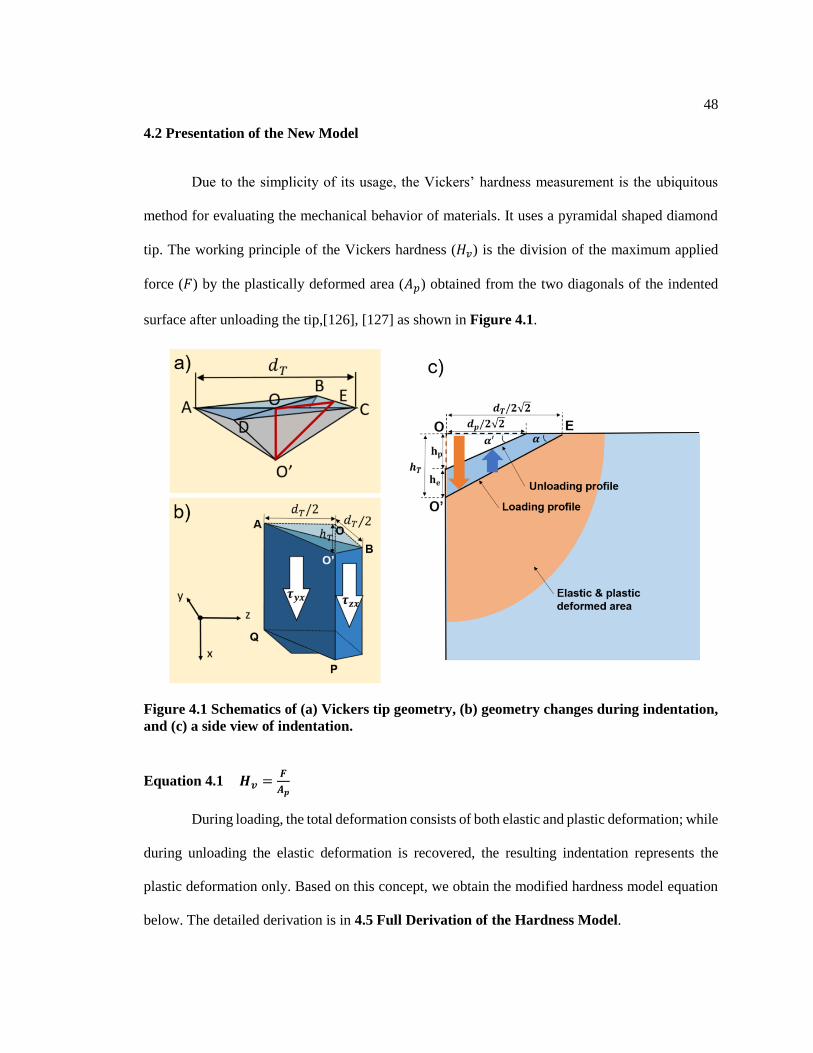
48
4.2 Presentation of the New Model
Due to the simplicity of its usage, the Vickers’ hardness measurement is the ubiquitous
method for evaluating the mechanical behavior of materials. It uses a pyramidal shaped diamond
tip. The working principle of the Vickers hardness (𝐻𝑣) is the division of the maximum applied
force (𝐹) by the plastically deformed area (𝐴𝑝) obtained from the two diagonals of the indented
surface after unloading the tip,[126], [127] as shown in Figure 4.1.
Figure 4.1 Schematics of (a) Vickers tip geometry, (b) geometry changes during indentation,
and (c) a side view of indentation.
Equation 4.1 𝑯𝒗 =𝑭
𝑨𝒑
During loading, the total deformation consists of both elastic and plastic deformation; while
during unloading the elastic deformation is recovered, the resulting indentation represents the
plastic deformation only. Based on this concept, we obtain the modified hardness model equation
below. The detailed derivation is in 4.5 Full Derivation of the Hardness Model.
49
Equation 4.2 𝑯𝒗 = 𝒄 𝑮 (𝒉𝑻
𝒉𝒑)𝟐
𝐭𝐚𝐧𝟑/𝟐𝜶 𝐜𝐨𝐬 𝜶
where ℎ𝑇 and ℎ𝑝 are the indentation depths at the maximum loading and after unloading,
respectively; 𝛼 is the angle of the indenter tip (𝛼 = 22° for a Vickers diamond tip), 𝐺 is the shear
modulus of the material, and 𝑐 is a scaling factor.
In this model, we closely look into ℎ𝑇/ℎ𝑝 ratio values in the load-displacement curves of
Vickers and Berkovich hardness measurements[127]–[130]. For purely plastic materials, ℎ𝑇/ℎ𝑝 =
1, and for purely elastic materials, ℎ𝑇/ℎ𝑝 = ∞. Different from prior approaches is evident in the
fact that the ℎ𝑇/ℎ𝑝 ratio is equivalent to the dissipated energy ratio between (elastic+plastic) and
plastic deformations. Most critical to the new model, and what follows is the estimation of the
plastic energy, which originates from dislocation energy, and plays a significant role in this model.
For capturing the dislocation energy, the concept of flow stress is introduced. After modeling the
ℎ𝑇/ℎ𝑝 ratio and scaling factor c, Equation 4.3 was obtained.
Equation 4.3 𝑯𝒗 = 𝟎. 𝟏𝟔𝟏𝟓 𝑮 (𝟏 +𝟖𝟎𝟎𝟎
𝟑
𝒘
𝒃(𝒃
𝒔)𝟐(𝝉𝑷𝑵
𝑮)𝟐)𝟐
𝒆−𝟐.𝟐𝒌 (𝒃
𝒔)𝟒𝐭𝐚𝐧𝟑/𝟐 𝒂𝐜𝐨𝐬𝒂
where 𝜏𝑃𝑁 and 𝑤 are the Peierls-Nabarro stress and dislocation width, respectively, 𝑏/𝑠 is the
Burgers vector and slip plane spacing, and 𝑘 is the ratio of shear and bulk moduli. A detailed
derivation is shown in 4.5 Full Derivation of the Hardness Model.
4.3 Validation and Prediction
In the present hardness model, the active slip systems, 𝑏/𝑠, and dislocation width, 𝑤, of
materials as well as their elastic properties and melting temperatures constitute the input data.
Typically, in a crystalline material there are many slip systems that coexist, but specific slip systems
are activated at a given condition. The active slip systems of materials can be determined not only

50
by the crystal structures but also by materials’ bonding nature such as the electronic structure of
materials[131]. Note, for the purposes of this model, we will only consider the material hardness at
room temperature. Furthermore, the active slip system in a material usually is accompanied by
other equivalent slip systems (typically more than one). For example, typical active slip systems of
the diamond cubic structure are shuffle and glide, and those of body centered cubic (BCC) structure
are ½ [111]{110}, ½ [111]{211} and ½ [111]{321} slip systems. Therefore, the active slip systems
can be determined by portions of the energetic descriptions of each slip system. The present model
has considered the major active slip systems of each structure shown in Table 4.1.
Table 4.1 Slip systems of different crystal structures.
Structur
e
Dislocatio
n type
Burgers
vector, �� �� length, b
Slip
plane Interspacing, s
example
FCC edge 1
2[110] 𝑎0/√2 {111} √(
√3𝑎03)
2
+ (√3𝑎03)
2
Ni, Al,
Au, Ir, Rh
FCC screw 1
2[110] 𝑎0/√2 {110}
1
2√𝑎02 + (
√2𝑎02)
2
Ir, Rh
BCC screw 1
2[111] 𝑎0√3/2 {110}
√2𝑎0
√3
Mo, V,
Fe, W
BCC screw 1
2[111] 𝑎0√3/2 {211}
𝑎0
√2 Nd, W
HCP-
basal edge
1
3[1210] 𝑎0 {0001}
𝑐
2
Mg, Zn,
Cd
HCP-
prism edge
1
3[1210] 𝑎0 {1010}
√3𝑎02
Ti, Zr
HCP-
pyramidal edge
1
3[1210] 𝑎0 {1011}
1
√43(1𝑎0)2
+ (1𝑐)2
Co
HCP-
twin edge
1
2[1011]
1
2√𝑎0
2 + 𝑐2 {1012}
1
√43(1𝑎0)2
+ (2𝑐)2
Be
Diamon
d cubic edge
1
2[110] 𝑎0/√2 {111} √(
√3𝑎06)
2
+ (√3𝑎06)
2
C(diamon
d), Si, Ge

51
Diamon
d cubic screw
1
2[110] 𝑎0/√2 {111} √(
√3𝑎06)
2
+ (√3𝑎06)
2
Si, Ge
Zinc
blende edge
1
2[110] 𝑎0/√2 {111} √(
√3𝑎06)
2
+ (√3𝑎06)
2
SiC,
ZnSe,
ZnS
Zinc
blende edge
1
2[110] 𝑎0/√2 {110} √(
√2𝑎04)
2
+ (√2𝑎04)
2
ZnSe,
ZnS
Rocksal
t edge
1
2[110] 𝑎0/√2 {111} √(
√3𝑎06)
2
+ (√3𝑎06)
2
TiC, TiN,
ZrC
Rocksal
t edge
1
2[110] 𝑎0/√2 {110} √(
√2𝑎04)
2
+ (√2𝑎04)
2
MgO
Spinel edge 1
2[110] 𝑎0/√2 {111} √(
√3𝑎06)
2
+ (√3𝑎06)
2
MgAl2O4
We will review our results for each crystallographic system. Face-centered cubic (FCC)
metals are ductile with low flow stresses, resulting in their ℎ/ℎ𝑝 ratios being close to 1. The active
slip system of FCC metals at room temperature is mainly ½ [110]{111} since the most densely
packed planes of FCC metals are {111}[132]. The calculated hardness values from the present
hardness model are in good agreement with experimental data except for Ir, Rh, and Th[132], [133]
as shown in Figure 4.2a. Although the crystal structures of Ir and Rh are FCC, their slip systems
are complex since both planar and non-planar core structures can coexist[134], [135]. Through
atomistic simulations using a bond-order potential Cawkwell et al.[131] found that the non-planar
core structure is due to the ½ [110] screw dislocation originating from unsaturated d-bonds. This
aspect of interatomic bonding distinguishes Ir, Rh, and Th from most other FCC metals. The present
model can predict the hardness with different slip systems as shown in Figure 4.2a for Ir, Rh, and
Th, and the actual deformation process is likely a result of a mixture of various slip systems.

52

53
Figure 4.2 Hardness comparisons of (a) FCC, (b) BCC, and (c) HCP materials with respect
to experimental data. Solid and open symbols represent the predicted values using elastic
properties from experiments and first-principles calculations. Red dashed lines indicate value
equality, vertical dotted lines connect the hardness between the slip systems.
BCC metals are usually brittle due to the higher flow stress of screw dislocations, resulting
in higher hardness values than other metals as shown in Figure 4.2b. The active slip systems of
BCC structures at room temperature are either or combinations of ½ [111]{110}, ½ [111]{211} and
½ [111]{321} screw dislocations[136]. The active slip system of Mo[137], Fe[138], V[139], and
Cr[140] at room temperature is the ½ [111]{110} screw dislocation, while those of Nb[136], [141]
and W[136], [142] at room temperature consist of both ½ [111]{110} and ½ [111]{211} screw
dislocations. Based on the calculated hardness from the present model, the active slip systems of
W are predicted to be the mixture of ½ [111]{110} and ½ [111]{211} screw dislocations. The active
slip systems of BCC metals predicted by the present model agree well with those observed
experimentally as shown in Table 4.2. It should be noted that in general the active slip systems
change with the operating temperature. This is especially true for Nb and W; the active slip systems
of Nb and W at room temperature are different from those at 77 K[136]. The prediction of
temperature dependence of hardness will be discussed in subsequent chapter.
Table 4.2 Slip systems at room temperature in BCC metals.
Model W Mo Nb Fe V Cr
This model
prediction 110, 211 110 110, 211 110 110 110
Weinberger et
al.[136] 110, 211
110,
some 211 110 110 110, 211 -
Fritz et al.[140] - - - - - 110
Bressers et
al.[139] - - - -
110,
Rarely 211 -
Schadler et
al.[143] 110, 211 - - - - -
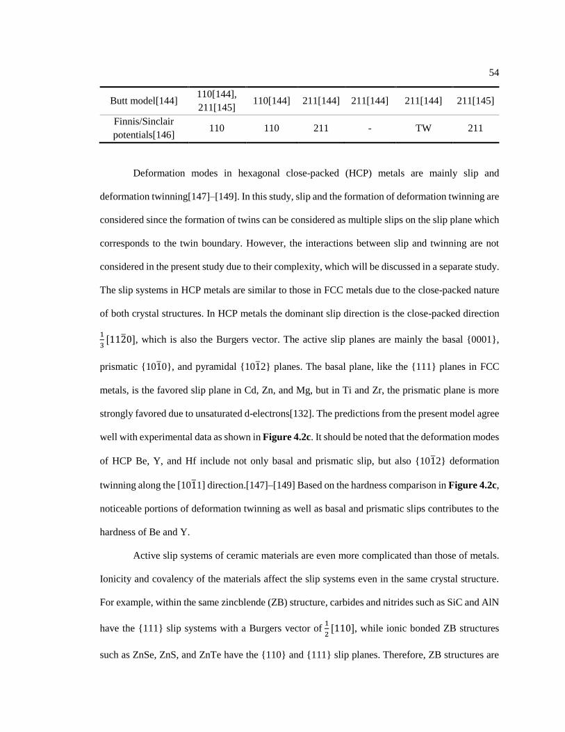
54
Butt model[144] 110[144],
211[145] 110[144] 211[144] 211[144] 211[144] 211[145]
Finnis/Sinclair
potentials[146] 110 110 211 - TW 211
Deformation modes in hexagonal close-packed (HCP) metals are mainly slip and
deformation twinning[147]–[149]. In this study, slip and the formation of deformation twinning are
considered since the formation of twins can be considered as multiple slips on the slip plane which
corresponds to the twin boundary. However, the interactions between slip and twinning are not
considered in the present study due to their complexity, which will be discussed in a separate study.
The slip systems in HCP metals are similar to those in FCC metals due to the close-packed nature
of both crystal structures. In HCP metals the dominant slip direction is the close-packed direction
1
3[1120], which is also the Burgers vector. The active slip planes are mainly the basal {0001},
prismatic {1010}, and pyramidal {1012} planes. The basal plane, like the {111} planes in FCC
metals, is the favored slip plane in Cd, Zn, and Mg, but in Ti and Zr, the prismatic plane is more
strongly favored due to unsaturated d-electrons[132]. The predictions from the present model agree
well with experimental data as shown in Figure 4.2c. It should be noted that the deformation modes
of HCP Be, Y, and Hf include not only basal and prismatic slip, but also {1012} deformation
twinning along the [1011] direction.[147]–[149] Based on the hardness comparison in Figure 4.2c,
noticeable portions of deformation twinning as well as basal and prismatic slips contributes to the
hardness of Be and Y.
Active slip systems of ceramic materials are even more complicated than those of metals.
Ionicity and covalency of the materials affect the slip systems even in the same crystal structure.
For example, within the same zincblende (ZB) structure, carbides and nitrides such as SiC and AlN
have the {111} slip systems with a Burgers vector of 1
2[110], while ionic bonded ZB structures
such as ZnSe, ZnS, and ZnTe have the {110} and {111} slip planes. Therefore, ZB structures are

55
divided into ionic and covalent ZB structures. Furthermore, the active slip systems of NaCl
structures are the same as those of ZB structures, i.e., the {111} slip system for carbide and nitride
NaCl structures such as TiN and Ti,C, and the {110} and {001}slip systems[150]–[152] for ionic
bonded NaCl structures such as MgO and NaCl, respectively.
Similarly, understanding of slip systems of semiconductor materials is crucial for
determining dislocation behavior and plastic deformation during epitaxial growth and device
processing in order to improve their optical and electronical properties and homogeneity[153].
Zincblende and diamond cubic crystal structured semiconductor materials have two major slip
systems, which are glide edge and shuffle screw dislocations[154]–[156]. The present model is
capable of predicting the energetic contribution of each active slip system on hardness. It is known
that the active slip systems in semiconductor materials such as Si and GaAs are combinations of
glide edge and shuffle screw dislocations,[154]–[156] where the zig-zag shaped 1
6[121] partial
dislocations of the glide-set in ZB and diamond cubic crystal structures can be treated as a 1
2[110]
full dislocation in the present model. As shown in Figure 4.3, the experimental hardness values of
the semiconductor materials such as GaAs, GaP, and AlSb are in between the predicted values from
these glide edge and shuffle screw slip systems. This indicates that the glide-set and shuffle-set slip
systems coexist during the indentation process, but the hardness contribution from shuffle screw
dislocations is much smaller than those from glide edge dislocations. The experimental hardness
values (12 and 8.8 GPa) of Si and Ge seem to be located in between the contributions of glide-set
(8.6 and 5.3 GPa) and shuffle-set (28.5 and 13.8 GPa) slips, respectively. If only contributions from
these two sets of slip types, the glide-set of slip is dominant, representing 83% and 59% of the total
hardness for Si and Ge, respectively, though the possible phase transformation to a tetragonal β-tin
structure during indentation process between 0 and 300 °C[157]–[159] with pop-out or elbow in
the load-displacement curve could potentially complicate the situation. Furthermore, the

56
quantitative contributions from the individual slip systems would also depend on the migration
barrier of the dislocation in terms of possible kink formation and migration[160].
0 5 10 150
10
20
3040
45
Si
ZnS
ZnSe
ZnTe InSb
GaSb
AlSb
InAs
AlAs
InP
GaAs
Ge
AlP
GaP
Expt. G&B Glide
Calc. G&B Glide
Expt. G&B Shuffle
Calc. G&B Shuffle
Mo
de
lle
d H
v (
GP
a)
Experimental Hv (GPa)
Figure 4.3 Hardness comparisons of ceramic materials with respect to experimental data.
Solid and open symbols represent the predicted values using elastic properties from
experiments and first-principles calculations. Red dashed lines indicate value equality,
vertical dotted lines show the differences between glide edge and shuffle screw slip systems.
4.4 Discussion
It is known that the indentation hardness represents the materials’ ability to resist plastic
deformation. The lack of materials’ properties on the imparted plastic deformation in existing
hardness models in the literature has limited the predictive capability of these models. It is noted
that the Vickers and Berkovich hardness tests use a slow and fixed loading rate to avoid the effects
of impact and strain rate,[161] thus enabling the use of the static attributes of plastic deformation
in the present hardness model, including the Peierls-Nabarro flow stress, dislocation width, Burgers
vector, and slip plane spacing in addition to the elastic properties conventionally used in existing
hardness models. Based on the well-established concept of active slip systems during plastic

57
deformation, the present model captures the competition among possible slip systems among pure
elements and compounds originating from their unsaturated d-bonds[131].
With model parameters evaluated from available experimental data in the literature, the
present model is able to satisfactorily cover the hardness ranges from 0.1 GPa of pure metals to 100
GPa of ceramic materials as shown in Figure 4.4. For materials with more than one slip system
being activated, the apparent hardness values seem to fall between the hardness values of the
activated slip systems. Figure 4.5 and Table 4.3 further shows that the PN flow stress decreases
exponentially with increasing dislocation width, and the PN flow stress agrees well with
experimentally determined yield stress at low temperature.
0 20 40 60 80 100 120
0
20
40
60
80
100
120
0 2 4 6 8 100
2
4
6
8
10
From Expt. G&B
From Calc. G&B
Mo
de
lled
Hv (
GP
a)
Experimental Hv (GPa)
Figure 4.4 Hardness comparisons of all tested materials with respect to experimental data.
Solid and open symbols represent the predicted values using elastic properties from
experiments and first-principles calculations. The experiments for all materials both
hardness and elastic properties data from Table 4.6. Red dashed lines indicate value equality.

58
0.4 0.6 0.8 1.0 1.2 1.4 1.6 1.8 2.0 2.2 2.4
10-6
10-5
10-4
10-3
10-2
10-1
100
Dislocation width, w0K
Flo
w o
r Y
ield
str
ess, P
N/G
or Y
/G
Expt. Y/G at low T
Diamond C and Si
BCC metals
FCC metals
HCP metals
Calc. PN/G at 0K
Carbides or Nitrides
Semiconductors
Other ceramics
BCC metals
FCC metals
HCP metals
Figure 4.5 Comparison of Peierls-Nabarro flow stress at 0 K with experimental yield stress
at low temperatures (4~77K) as a function of dislocation width. Data and references are listed
in Table 4.3.
Table 4.3 Comparison of PN flow stress at 0K with experimental yield stress (𝝉𝒀
𝑮) at low
temperatures (4~77 K) as a function of dislocation width.
Material Structure 𝝉𝑷𝑵𝑮
𝝉𝒀𝑮
References
C Diamond cubic 2.34 × 10⁻² 5.71 × 10⁻² [162]
Si Diamond cubic
1.21 × 10⁻² ~2.66× 10⁻²
1.00 × 10⁻¹ [163]
Fe BCC 2.67 × 10⁻³ 5.50 × 10⁻³ [164]
Mo BCC 2.67 × 10⁻³ 5.11 × 10⁻⁴ [165], [166]
Nb BCC 2.67 × 10⁻³ 8.80 × 10⁻⁴ [165]
Al FCC 2.23 × 10⁻⁵ 1.09 × 10⁻⁵ [165]
Al FCC 4.00 × 10⁻⁵ [167]
Ni FCC 4.28 × 10⁻⁵ 6.58 × 10⁻⁵ [165]
Cu FCC 2.33 × 10⁻⁵ 5.31 × 10⁻⁶ [165]
Cu FCC 1.04 × 10⁻⁵ [168]
Ag FCC 1.60 × 10⁻⁵ 2.00 × 10⁻⁵ [169]
Ag FCC 2.60 × 10⁻⁵ [170]
Be HCP (basal
slip) 6.26 × 10⁻³ 7.16 × 10⁻⁴ [171]

59
Be HCP (prism
slip) 3.67 × 10⁻³ 1.35 × 10⁻³ [165]
Mg HCP 1.07 × 10⁻³ 1.00 × 10⁻⁴ [172]
Mg HCP (prism
slip) 6.65 × 10⁻⁴ 2.00 × 10⁻³ [165]
Cd HCP (basal
slip) 1.83 × 10⁻⁴ 2.10 × 10⁻⁵ [173]
Zn HCP 5.00 × 10⁻⁴ 2.00 × 10⁻⁵ [174]
Ti HCP 4.60 × 10⁻⁴ 1.16 × 10⁻³ [175]
Ti HCP 1.74 × 10⁻³ [175]–[177] 𝜏𝑃𝑁
𝐺 was calculated from Equation 4.27 or Equation 4.28 with the information in Table 4.6.
As discussed in detail in 4.5 Full Derivation of the Hardness Model, the ℎ𝑇/ℎ𝑝 ratio
equals the ratio of the total energy and plastic energy dissipated during the indentation, i.e., 𝐸𝑇/𝐸𝑝.
This energy ratio can be correlated with the plasticity index[178] or the indentation ductility
index[179]. In the present work, we define the indentation ductility index as follows with the details
presented in 4.5 Full Derivation of the Hardness Model.
Equation 4.4 𝑫 =𝑬𝒑
𝑬𝒆=𝒉𝒑
𝒉𝒆=
𝟏
𝟖𝟎𝟎𝟎
𝟑
𝒘
𝒃(𝒃
𝒔)𝟐(𝝉𝑷𝑵𝑮)𝟐
where 𝐸𝑒 and ℎ𝑒 are the elastic energy and elastic deformation depth during indentation,
respectively. Figure 4.6 plots 𝐷 with respect to the dislocation width at room temperature. For
highly plastic materials, i.e., ductile materials, 𝐷 approaches ∞, while for highly elastic materials
𝐷 approaches zero.

60
0.4 0.6 0.8 1.0 1.2 1.4 1.6 1.8 2.0 2.2 2.410
-1
101
103
105
107
109
Carbides and Nitrides
Semiconductors
other cubic ceramics
BCC metals
FCC metals
HCP metalsIn
denta
tion
du
ctilit
y inde
x, D
Dislocation width, w
Figure 4.6 Indentation ductility index as a function of dislocation width at room temperature.
Finally, it is important to recognize that the power of the present hardness model is in its
ease of expandability to a more comprehensive hardness model which includes the effects of
temperature, grain size or twin boundary thickness, and solute atom size. For example, the
temperature dependent hardness, i.e., hot hardness, can be calculated based on the temperature
dependence of the PN flow stress and dislocation width; therefore, these factors can be possibly
included in the extended model. The details will be discussed in future publications.
4.5 Full Derivation of the Hardness Model
4.5.1 Derivation of the Hardness Equation
The Vickers hardness is defined as follows:

61
Equation 4.5 𝑯𝒗 =𝑭𝒎𝒂𝒙
𝑨𝒑
where 𝐹𝑚𝑎𝑥 is the maximum applied force, and 𝐴𝑝 the plastically deformed area after the indenter
tip is unloaded (see Figure 4.1a). 𝐴𝑝 can be obtained from the resulting indentation as follows[180]
Equation 4.6 𝑨𝒑 =𝒅𝒑𝟐
𝟐 𝐜𝐨𝐬 𝒂′
where 𝑑𝑝 is the diagonal length of the resulting indentation on the sample surface, and 𝛼′ the angle
between the sample surface and the indented surface after unloading the tip. (△ABO’ in Figure
4.1b).
To estimate the applied maximum force, 𝐹𝑚𝑎𝑥, we assume that the pyramid indentation can
be divided into four triangular pyramid indenters and each part is a pure shear process[181] with
two forces acting on xz(𝜏𝑦𝑥) and xy(𝜏𝑧𝑥) planes, respectively, as shown in Figure 4.1b. As the
indentation process contains both elastic and plastic deformations, 𝐹𝑚𝑎𝑥 can be written as
follows[182]
Equation 4.7 𝑭𝒎𝒂𝒙 = 𝑨𝑻𝝉𝑻
where 𝐴𝑇 is the shear area, parallel to the applied force during loading, and 𝜏𝑇 the total shear stress,
both at maximum loading[182]. The shear area is the parallelogram marked by AO’PQ in Figure
4.1b. It is a complex quantity due to the difficulty in determining the elastic deformation depth
(𝑂′𝑃 in Figure 4.1b), which includes the small atomic displacements by a single dislocation
nucleation and reaches further down to the depth of the orange colored area in Figure 4.1c. The
shear area is conventionally assumed to be proportional to the deformed area (△AOO’ in Figure
4.1b) of the indentation during loading[181] with a material dependent coefficient, i.e.,
Equation 4.8 𝑨𝑻 =𝟏
𝟐𝒄𝟏𝒅𝑻
𝟐 𝐭𝐚𝐧𝜶
where 𝑑𝑇 is the diagonal length of the indentation at maximum loading, 𝛼 the angle between the
sample surface and indented surface during indentation, being 22o for a Vickers diamond tip, and

62
𝑐1 the material dependent coefficient representing the complexity in determining the shear area to
be discussed later.
In various indentation techniques including spherical and Vickers indentations,[183]–[191]
typical shear stress-strain curves follow approximately the Taylor relation[192]–[194] as follows
Equation 4.9 𝝉𝑻 = 𝒄𝟐𝑮√𝜸𝑻
as shown in Figure 4.7 with 𝑐2 being a geometrical factor, 𝐺 the elastic shear modulus, and 𝛾𝑇 the
total shear strain dictated by the geometry of the indentation tip as shown below
Equation 4.10 𝜸𝑻 =𝒉𝑻
𝒅𝑻= 𝐭𝐚𝐧𝜶
where ℎ𝑇 is the indentation depth at maximum loading.
Figure 4.7 (a) Stress(𝝉 )-strain(𝜸 ) curve during shear deformation. (b) typical Load(F)-
displacement(h) curve during indentation process.
By inserting Equation 4.8, Equation 4.9 and Equation 4.10 into Equation 4.7, the
applied force is obtained
Equation 4.11 𝑭𝒎𝒂𝒙 =𝟏
𝟐𝒄 𝑮 𝒅𝑻
𝟐𝒕𝒂𝒏𝟑/𝟐𝜶
where 𝑐 = 𝑐1𝑐2 to be discussed in section 4.5.2.2 Parameter c.
Based on Equation 4.6 and Equation 4.11, Equation 4.5 can be re-organized as follows
Equation 4.12 𝑯𝒗 = 𝒄 𝑮 (𝒅𝑻
𝒅𝒑)𝟐
𝒕𝒂𝒏𝟑/𝟐𝜶 𝒄𝒐𝒔 𝜶′

63
where 𝑑𝑝 is the diagonal length of the indentation due to the plastic deformation after unloading
the indentation tip (see Figure 4.1c).
The term 𝑑𝑇/𝑑𝑝 can be re-expressed as the indentation depth, ℎ𝑇 tan𝛼
′
ℎ𝑝 tan𝛼, from the geometry
of the tip (Equation 4.10) and indented surface (ℎ𝑝 = 𝑑𝑝 tan𝛼′) where ℎ𝑝 is the depth of the
indentation due to the plastic deformation after unloading the indentation tip. It can be seen if 𝛼′
equals to 𝛼 , 𝑑𝑇/𝑑𝑝 equals to ℎ𝑇/ℎ𝑝 , i.e., the ratio between the total deformation and plastic
deformation is the same on the sample surface and along the indentation depth. This is an
approximation commonly used in the literature[195]–[197] and also adopted in the present work,
i.e.,
Equation 4.13 𝜶 ≈ 𝜶′
It should be noted that the error introduced by the above approximation is partially canceled when
𝑐 in Equation 4.11, is evaluated, see section 4.5.2.2 Parameter c. Therefore, Equation 4.12 can
be re-written as follows
Equation 4.14 𝑯𝒗 = 𝒄 𝑮 (𝒉𝑻
𝒉𝒑)𝟐
𝒕𝒂𝒏𝟑/𝟐𝜶 𝒄𝒐𝒔 𝜶
4.5.2 Evaluation of Model Parameters
4.5.2.1 𝒉𝑻/𝒉𝒑 Ratio
For modelling of ℎ𝑇
ℎ𝑝 in Equation 4.14, we collected experimentally measured hardness
(𝐻𝑣) and load-displacement (F-h) curves in the literature as listed in Table 4.4 including pure
metals and ceramic materials, with ℎ𝑇 and ℎ𝑝 denoted by the intercepts on the x-axis at maximum
load and after unloading, respectively, as shown in Figure 4.8a. Both Vickers and Berkovich
hardness data are considered because the hardness values from Vickers hardness (four face
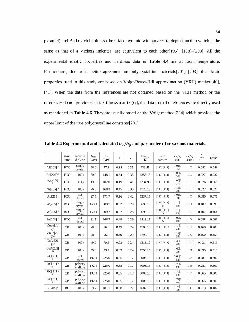
64
pyramid) and Berkovich hardness (three face pyramid with an area to depth function which is the
same as that of a Vickers indenter) are equivalent to each other[195], [198]–[200]. All the
experimental elastic properties and hardness data in Table 4.4 are at room temperature.
Furthermore, due to its better agreement on polycrystalline materials[201]–[203], the elastic
properties used in this study are based on Voigt-Reuss-Hill approximation (VRH) method[40],
[41]. When the data from the references are not obtained based on the VRH method or the
references do not provide elastic stiffness matrix (cij), the data from the references are directly used
as mentioned in Table 4.6. They are usually based on the Voigt method[204] which provides the
upper limit of the true polycrystalline constants[201].
Table 4.4 Experimental and calculated 𝒉𝑻/𝒉𝒑 and parameter c for various materials.
structure
indented plane
Ghkl (GPa)
B (GPa)
k v TMelting
(K) slip
system
ℎ𝑇/ℎ𝑝
(exp.)
ℎ𝑇/ℎ𝑝
(calc.)
c
(exp.
)
c
(calc.
)
Al[205],B FCC single
crystal 26.0 77.3 0.34 0.35 933.45 [110]{111}
1.01[1
95] 1.00 0.042 0.046
Cu[205],B FCC (100) 50.9 148.1 0.34 0.35 1358.15 [110]{111} 1.05[2
06] 1.00 0.027 0.032
Ag[205],
B FCC (111) 19.3 102.0 0.19 0.41 1234.95 [110]{111}
1.06[2
07] 1.00 0.076 0.069
Ni[205],B FCC (100) 76.0 168.3 0.45 0.30 1728.15 [110]{111} 1.13[2
08] 1.00 0.027 0.027
Au[205] FCC not
listed 27.5 171.7 0.16 0.42 1337.15 [110]{111}
1.01[2
09] 1.00 0.080 0.075
W[205],B BCC single
crystal 160.0 309.7 0.52 0.28 3695.15
[111]{211}
S
1.15[1
95] 1.01 0.107 0.093
W[205],B BCC single crystal
160.0 309.7 0.52 0.28 3695.15 [111]{110}
S
1.15[1
95] 1.09 0.107 0.168
Fe[205],V BCC not
listed 81.5 166.7 0.49 0.29 1811.15
[111]{110}
S
1.02[2
10] 1.01 0.088 0.090
ZnSe[205],B
ZB (100) 28.0 56.6 0.49 0.29 1798.15 [110]{110} 1.14[1
28] 1.04 0.160 0.202
ZnSe[20
5],B ZB (100) 28.0 56.6 0.49 0.29 1798.15 [110]{111}
1.14[1
28] 1.43 0.160 0.454
GaAs[205],B
ZB (100) 49.5 79.9 0.62 0.24 1511.15 [110]{111} 1.49[1
28] 1.60 0.421 0.310
GaP[205],B
ZB (100) 59.3 93.7 0.63 0.24 1750.15 [110]{111} 1.60[1
28] 1.67 0.395 0.313
SiC[211],
B ZB
not listed
192.0 225.0 0.85 0.17 3003.15 [110]{111} 2.04[2
12] 1.95 0.281 0.307
SiC[211],
B ZB
polycry
stalline 192.0 225.0 0.85 0.17 3003.15 [110]{111}
1.79[2
13] 1.95 0.281 0.307
SiC[211],
V ZB
polycrystalline
192.0 225.0 0.85 0.17 3003.15 [110]{111} 1.79[2
13] 1.95 0.365 0.307
SiC[211],
V ZB
polycry
stalline 192.0 225.0 0.85 0.17 3003.15 [110]{111}
1.72[2
10] 1.95 0.365 0.307
Si[205],B DC (100) 69.2 101.1 0.68 0.22 1687.15 [110]{111} 2.26[1
28] 1.48 0.313 0.404

65
Si[205],B DC (100) 69.2 101.1 0.68 0.22 1687.15 [110]{111}
S
2.26[1
28] 3.47 0.313 0.444
c-
BN[214],
B ZB (111) 405.4 399.7 1.01 0.12 3246.15 [110]{111}
2.50[2
12] 2.42 0.162 0.200
BC2N[21
5],B ZB
not
listed 445.0 408.0 1.09 0.10 3273.15 [110]{111}
2.85[2
12] 2.52 0.139 0.184
MgO[205],V
NaCl polycrystalline
130.0 160.0 0.81 0.18 3125.15 [110]{100} 1.16[2
10] 1.09 0.225 0.150
MgAl2O4
[210],V
spine
l
polycry
stalline 96.0 180.0 0.53 0.27 2408.15 [110]{111}
1.47[2
10] 1.35 0.427 0.602
*B and V in column 1 for Berkovich and Vickers indentation methods, respectively.
Figure 4.8 Typical Load-displacement curves (a) F-h curve and (b) √𝑭-h curve. Red lines are
loading curves and blue lines are unloading curves, and green dot line represents only the
plastic contribution from Equation 4.16.
As shown by Sakai et al.,[210], [213] there is a linear relationship between the square root
of the load and displacement, i.e., √𝐹 ∝ ℎ, as shown in Figure 4.8b. Moreover, Oliver et al.[130],
[195] also observed this relationship for the pyramid shaped indenter. Using the Maxwell
combination of the elastic and plastic elements in a viscoelasticity model, the following equations
can be obtained[216]
Equation 4.15 𝒉𝑻 = 𝒉𝒑 + 𝒉𝒆
Equation 4.16 𝑭𝒎𝒂𝒙 = 𝒌𝑻𝒉𝑻𝟐 = 𝒌𝒆𝒉𝒆
𝟐 = 𝒌𝒑𝒉𝒑𝟐

66
where 𝑘𝑇 , 𝑘𝑒 , and 𝑘𝑝 are the coefficients for total, elastic, and plastic deformation, respectively,
and ℎ𝑒 is the indentation depth due to elastic deformation (see Figure 4.8a). The total, elastic, and
plastic deformation energies, 𝐸𝑇, 𝐸𝑒 , and 𝐸𝑝, correspond to the areas in a F-h curve[217]–[221] as
shown in Figure 4.8a and are related by the following equation.
Equation 4.17 𝑬𝑻 = ∫ 𝑭𝒅𝒉𝒉𝑻𝟎
=𝒌𝑻𝒉𝑻
𝟑
𝟑= 𝑬𝒆 + 𝑬𝒑 =
𝒌𝒆𝒉𝒆𝟑
𝟑+𝒌𝒑𝒉𝒑
𝟑
𝟑=𝑭𝒎𝒂𝒙
𝟑(𝒉𝒆 + 𝒉𝒑)
The ℎ𝑇
ℎ𝑝 ratio can thus be expressed in terms of the energy ratio as follows[222]–[224]
Equation 4.18 𝒉𝑻
𝒉𝒑= 𝟏 +
𝒉𝒆
𝒉𝒑= 𝟏 +
𝑬𝒆
𝑬𝒑
From the Frenkel’s classical elastic theory,[225], [226] the elastic shear strain of a defect-
free material is written as 𝛾𝑒 =𝑏
2𝜋𝑠, and the corresponding elastic energy can be calculated by the
following equation
Equation 4.19 𝑬𝒆 =𝟏
𝟐𝑮𝑽𝒆𝜸𝒆
𝟐 =𝟏
𝟐𝑮𝑽𝒆 (
𝒃
𝟐𝝅𝒔)𝟐
where 𝑉𝑒 is the volume of elastic deformation during indentation, b the Burgers vector, and s the
interplanar spacing of the slip plane. The obtained b and s from crystal structures are listed in Table
4.1.
Since plastic deformation is mainly due to dislocations, the plastic deformation energy in the
present work is calculated from the average dislocation line energy of 𝐺𝑏2 as follows[227]
Equation 4.20 𝑬𝒑 ≈ 𝝆𝑻𝑽𝒑𝑮𝒃𝟐
where 𝜌𝑇 and 𝑉𝑝 are the total dislocation density generated by the indentation process and the
plastic deformation volume during indentation, respectively. 𝜌𝑇 contains both statistically stored
dislocation density (𝜌𝑆𝑆𝐷) which is due to the multiplication of dislocations by the deformation and
geometrically necessary dislocation density (𝜌𝐺𝑁𝐷) which is due to the required dislocations to
match plastic strain gradient.[194], [228] 𝜌𝑇𝑉𝑝 is the number of dislocations to fill up the plastic

67
deformation volume. Inserting Equation 4.19 and Equation 4.20 into Equation 4.18, we obtain
the ℎ
ℎ𝑝 ratio as follows
Equation 4.21 𝒉𝑻
𝒉𝒑= 𝟏 +
𝟏
𝟖𝝅𝟐𝝆𝑻𝒔𝟐
𝑽𝒆
𝑽𝒑
In the following, the evaluations of quantities in Equation 4.18 are discussed. Based on
the Taylor relation[192]–[194] the relation between stress and dislocation density can be written
as follows
Equation 4.22 𝝉 − 𝝉𝑷𝑵 = 𝒒𝑮𝒃√∆𝝆
where 𝜏𝑃𝑁 is the PN flow stress for dislocation gliding to start, 𝑞 a constant and ∆𝜌 is the
dislocation density difference by indentation process (∆𝜌 = 𝜌 − 𝜌0), where 𝜌0 initial dislocation
density before indentation. 𝜌0 is negligible compare to 𝜌𝑇 when the sample is not work-hardened.
To obtain the saturated hardness without the effect of indentation size due to the strain gradient
(𝜌𝑆𝑆𝐷 >> 𝜌𝐺𝑁𝐷), the applied maximum shear stress (𝜏𝑇) should be equal to or larger than the ideal
shear strength[229] which is the first maximum in the shear stress–strain curve[230].
Let us consider the initiation of ∆𝜌 with ∆𝜌 = 1/𝑚2 when the stress is slightly above the
PN stress, i.e., 𝜏 = (𝑧 + 1)𝜏𝑃𝑁 with z being a very small number. One obtains from Equation 4.22
Equation 4.23 𝒛𝝉𝑷𝑵 = 𝒒𝑮𝒃√𝟏/𝒎𝟐
Since 𝜏𝑇 ≫ 𝜏𝑃𝑁 as shown in Table 4.5 and Figure 4.9, Equation 4.22 can be approximated as
follows
Equation 4.24 𝝉𝑻 ≈ 𝒒𝑮𝒃√𝝆𝑻
which has the similar form of Equation 4.9. Dividing Equation 4.23 by Equation 4.24 and re-
arranging gives the following equation
Equation 4.25 𝝆𝑮𝑵𝑫 ≈𝟏(𝒎−𝟐)𝒃𝟐
𝒛𝟐𝟏
𝒃𝟐(𝝉𝑻
𝑮)𝟐(𝝉𝑷𝑵
𝑮)−𝟐

68
0.5 1.0 1.5 2.010
-6
10-5
10-4
10-3
10-2
10-1
Cu
PN
/G
Carbides & Nitrides
Semiconductors
other cubic ceramics
BCC
FCC
HCP
T/G
Diamond
cBN
BCC
FCC
PN
/G o
r T
/G a
t 0
K
Dislocation width at 0K, w0K
AlNb
Mo
cBNDiamond
Figure 4.9 Peierls-Nabarro flow stress (𝝉𝑷𝑵) and ideal shear stress (𝝉𝑻) at 4.7 K and 7 K in
terms of dislocation width (𝒘𝟎) from Refs.[231]–[234] shown in Table 4.3 and Table 4.5.
Table 4.5 Comparison of 𝝉𝑷𝑵
𝑮 and
𝝉𝑻
𝑮
Materials 𝜏𝑃𝑁𝐺
𝜏𝑇𝐺
C (diamond) 1.97× 10⁻² 0.17 (96.3GPa/548GPa) [231], [232]
c-BN 1.62 × 10⁻² 0.17 (70.5GPa/405.4GPa) [231]
Mo (BCC) 2.00 × 10⁻³ 0.13 (15.8GPa/124.2GPa) [233]
Nb (BCC) 1.87 × 10⁻³ 0.17 (6.4GPa/37.5GPa) [233]
Al (FCC) 6.80 × 10⁻⁶ 0.15 (3.8GPa/25.4GPa) [234]
Cu (FCC) 1.03 × 10⁻⁵ 0.09 (3.61GPa/40.9GPa) [234] 𝜏𝑃𝑁
𝐺 are calculated from Equation 4.27 or Equation 4.28 with the information from Table 4.3
and Table 4.6.
It can be seen in Table 4.5 and Figure 4.9 that 𝜏𝑇
𝐺 does not change much from diamond to FCC
elements,[231]–[234] while 𝜏𝑃𝑁
𝐺 varies exponentially from 0.02 for diamond to ~10−6 for FCC
elements. Then, Equation 4.25 can be approximated as

69
Equation 4.26 𝝆𝑮𝑵𝑫(𝒎−𝟐) =
𝒆
𝒃𝟐(𝝉𝑷𝑵
𝑮)−𝟐
where 𝑒 (=1(𝑚−2)𝑏2
𝑧2(𝜏𝑇
𝐺)2) is treated as a constant to be evaluated.
The PN flow stresses for edge and screw dislocations are expressed below[15], [235]
Equation 4.27 𝝉𝑷𝑵
𝑮(𝒆𝒅𝒈𝒆) =
𝟏
(𝟏−𝒗)𝐞𝐱𝐩 (
−𝟐𝝅𝒘
𝒃)
Equation 4.28 𝝉𝑷𝑵
𝑮(𝒔𝒄𝒓𝒆𝒘) = 𝐞𝐱𝐩 (
−𝟐𝝅𝒘
𝒃)
where 𝑤 is the dislocation width. Its temperature dependency is approximated in the literature as
follows[236]–[238]
Equation 4.29 𝒘 = 𝒘𝟎 (𝟏 +𝑻
𝟑𝑻𝑴)
where 𝑤0 is the dislocation width at 0 K, equal to 𝑠 for screw dislocations, and 𝑠/(1 − 𝑣) for edge
dislocations with 𝑣 being the Poisson’s ratio at low temperatures,[15] and 𝑇𝑀 the melting
temperature.
The atomic displacement by a single dislocation occurs anisotropically over a few lattice
layers along the Burgers vector direction on the slip plane,[239]–[241] and this deformation is
regarded as the elastic volume by a single dislocation and proportional to the dislocation
width[238], [242], [243]. Consequently, we propose that (𝑉𝑒
𝑉𝑝) ∝
𝑤
𝑏, and by inserting this into
Equation 4.21, we obtained as follows
Equation 4.30 𝒉𝑻
𝒉𝒑= 𝟏 +
𝟖𝟎𝟎𝟎
𝟑
𝒘
𝒃(𝒃
𝒔)𝟐(𝝉𝑷𝑵
𝑮)𝟐
where the constant, 8000
3(≈
1
8𝜋2𝑒
𝑉𝑒
𝑉𝑝
𝑏
𝑤) is evaluated from the measured data of
ℎ𝑇
ℎ𝑝 and the materials
property data in the equation. The calculated value of ℎ𝑇
ℎ𝑝 from Equation 4.30 are compared with
the experimental data in Table 4.4 and Figure 4.10, showing good agreement.

70
1.0 1.5 2.0 2.5 3.0 3.5 4.0
1.0
1.5
2.0
2.5
3.0
3.5
4.0
ZnSe{110}
ZnSe{111}
b-SiCc-BN
BC2N
Si(100)-glide
Calc
. h
T/h
p
Expt. hT/hp
Si(100)-shuffle
Figure 4.10 Comparison of 𝒉𝑻/𝒉𝒑 ratio between experiment from Table 4.4 and the present
model.
4.5.2.2 Parameter c
In the recent hardness modeling by Chen et al.[181], the model parameter 𝑐 in Equation
4.11 was assumed to be unity. Let us examine this assumption from experimental measurements
by re-organizing Equation 4.14 as follows
Equation 4.31 𝒄 =𝑯𝒗
𝑮(𝒉𝑻𝒉𝒑)𝟐
𝒕𝒂𝒏𝟑/𝟐𝜶 𝒄𝒐𝒔 𝜶
Table 4.4 lists the available experimental data and the calculated values of 𝑐 from the
above equation. It can be seen that 𝑐 varies more than an order of magnitude and thus needs to be
better modeled. In Table 4.4, the ratio of shear and bulk moduli, i.e., 𝑘 = 𝐺/𝐵 first used by
Pugh[123] and later used in the hardness modelling by Chen et al.[181], is also included along with
the slip systems and elastic properties.
71
Recently, Cheng et al.[244]–[247] derived an equation for the applied force during
indentation process using a scaling approach and revealed the approximate relationships between
hardness and elastic and plastic properties such as yield stress, elastic modulus, work hardening
exponent and Poisson’s ratio as follows
Equation 4.32 𝑭 = 𝑬𝒉𝟐∏(𝒀
𝑬, 𝝂, 𝒏, 𝜽)
with Y, E, 𝜈 , 𝑛, and 𝜃 being yield stress (flow stress in the present work), Young’s modulus,
Poisson’s ratio, work-hardening exponent, and indentation angle (𝑎 in the present study). It is
understood that 𝑌
𝐸 and 𝑛 are related to materials’ slip systems in terms of the Peierls-Nabarro flow
stress,[15], [235] 𝜈 is related to 𝑘 (=3(1−2𝑣)
2(1+𝑣)), and 𝑎 is fixed to 22° from the indentation tip angle.
Therefore, 𝑐 can be considered as a function of 𝑏
𝑠 and 𝑘.
Starting from the FCC pure metals with the same slip system ½ [110](111), 𝑏
𝑠= √3/2,
and ℎ𝑇
ℎ𝑝= 1, the following correlation is observed from Figure 4.11.
Equation 4.33 𝒄 ∝ 𝒆−𝟐.𝟐𝒌
The exponential relationship in Equation 4.33 is based on the relationship between Poisson’s ratio
and compressive stress found by Walsh[248] since 𝑘 is a function of Poisson’s ratio, and the
compressive stress is assumed to have the similar trend to the shear stress.

72
0.00 0.02 0.04 0.06 0.08 0.100.0
0.2
0.4
0.6
0.8
1.0
Ni
Cu
exp
(-2.2
k)
Expt. c
Al
Ag
Au
Figure 4.11 Exponential relationship of the scaling factor c (from Equation 4.31) for FCC
metals with data from Table 4.4.
To find out the relationship between 𝑏/𝑠 and 𝑐, the elastic shear energies from Equation
4.19 and from Equation 4.17 and Equation 4.11 are compared since the shear area A is mostly
from elastic deformation.
Equation 4.34 𝑬𝒆 =𝟏
𝟐𝑮𝑽𝒆 (
𝒃
𝟐𝝅𝒔)𝟐=𝒉𝒆
𝟑𝑭𝒎𝒂𝒙 =
𝒉𝒆
𝟑
𝟏
𝟐𝒄 𝑮 𝒅𝑻
𝟐𝒕𝒂𝒏𝟑/𝟐𝜶
with 𝑐 derived as
Equation 4.35 𝒄 =𝟑
𝟒𝝅𝟐𝑽𝒆
𝒅𝑻𝟐𝒉𝒆𝒕𝒂𝒏
𝟑/𝟐𝜶(𝒃
𝒔)𝟐
In Figure 4.12a, the values of 𝑐 evaluated from experimental data shown in Table 4.4 are plotted
with respect to (𝑏
𝑠)2, and a parabolic correlation is observed instead. Consequently, the following
relation is obtained, and the comparison between the calculated and experimental values of
parameter 𝑐 is plotted in Figure 4.12.
Equation 4.36 𝒄 = 𝟎. 𝟏𝟔𝟏𝟓 𝒆−𝟐.𝟐𝒌 (𝒃
𝒔)𝟒

73
Inserting Equation 4.30 and Equation 4.36 into Equation 4.14, we obtain the hardness
equation as follows
Equation 4.37 𝑯𝒗 = 𝟎. 𝟏𝟔𝟏𝟓 𝑮 (𝟏 +𝟖𝟎𝟎𝟎
𝟑
𝒘
𝒃(𝒃
𝒔)𝟐(𝝉𝑷𝑵
𝑮)𝟐)𝟐
𝒆−𝟐.𝟐𝒌 (𝒃
𝒔)𝟒𝐭𝐚𝐧𝟑/𝟐 𝒂𝐜𝐨𝐬𝒂
Figure 4.12 Plots of parameter c from experimental data (Equation 4.31) with data from
Table 4.4 (a) with respect to (𝒃/𝒔)𝟐 and (b) with respect to the model (Equation 4.36).

74
Table 4.6 Hardness comparison between the present and previous models with slip systems
and elastic properties with S for screw dislocation.
Compounds struc
ture G B k v
TMelting
(K) Slip system
Hv
calc. Hv exp.
Hv
Chen
[181]
H
Gao
[121
]
H
��im��nek[1
16]
C exp, [249] DC 578 443 1.30 0.05 3823.15 [110]{111} 100.
0 96±5[2
15] 109.7 93.6 95.4
C cal, [249] DC 548.3 465.5 1.18 0.08 3823.15 [110]{111} 100.
5 96±5[2
15] 93.9 93.6 95.4
C exp, [250],a DC 535.5 442.3 1.21 0.07 3823.15 [110]{111} 96.9 96±5[2
15] 95.7 93.6 95.4
C exp, [215] DC 535 443 1.21 0.07 3823.15 [110]{111} 96.9 96±5[2
15] 95.4 93.6 95.4
BC2N cal,
[251], b ORT 446 403 1.11 0.10 3273.15 [110]{111} 78.5 76[252] 76.9 78 71.9
BC2N exp,
[215] ORT 445 408 1.09 0.10 3273.15 [110]{111} 78.7 76[252] 75.4 78 71.9
c-BN exp,
[214],a ZB 405.4 400 1.01 0.12 3246.15 [110]{111} 72.8
66[253]
,
62[252]
,
63±5[2
15]
65.1 64.5 63.2
c-BN cal,
[249] ZB 403 404 1.00 0.13 3246.15 [110]{111} 72.5
66[253]
,
62[252]
,
63±5[2
15]
63.7 64.5 63.2
c-BN cal,
[249] ZB 382 376 1.02 0.12 3246.15 [110]{111} 68.5
66[253]
,
62[252]
,
63±5[2
15]
63.0 64.5 63.2
c-BN cal,
[254] ZB 405 384 1.05 0.11 3246.15 [110]{111} 72.0
66[253]
,
62[252]
,
63±5[2
15]
68.4 64.5 63.2
c-BN exp,
[215] ZB
409
±6
400
±3 1.02 0.12 3246.15 [110]{111} 73.3
66[253]
,
62[252]
,
63±5[2
15]
66.2 64.5 63.2
b-SiC exp,
[211] ZB 192 225 0.85 0.17 3003.15 [110]{111} 34.0
34[253]
,
28±3[2
15]
33.0 30.3 31.1
b-SiC cal,
[249] ZB 196.5 224.9 0.87 0.16 3003.15 [110]{111} 34.7
34[253]
,
28±3[2
15]
34.5 30.3 31.1
b-SiC cal,
[255] ZB 219 223 0.98 0.13 3003.15 [110]{111} 38.2
34[253]
,
28±3[2
15]
42.8 30.3 31.1
b-SiC exp,
[256] ZB 186.5 220.3 0.85 0.17 3003.15 [110]{111} 33.0
34[253]
,
28±3[2
15]
32.1 30.3 31.1
b-SiC exp,
[215] ZB
196
±13
226
±9 0.87 0.16 3003.15 [110]{111} 34.6
34[253]
,
28±3[2
15]
34.1 30.3 31.1
SiO2 exp,
[215]
stish
ovite 220 305 0.72 0.21 1983.15 [110]{111} 32.1
33±2[2
15] 29.0 30.4

75
SiO2 exp,
[215] stishovite
239 340 0.70 0.22 1983.15 [110]{111} 34.9 33±2[2
15] 29.6 30.4
VC cal, [181] NaCl 209.1 305.5 0.68 0.22 3083.15 [110]{111} 37.6 29[116] 26.2 27.2
ZrC exp,
[257],a NaCl 169.7 223.1 0.76 0.20 3805.15 [110]{111} 32.9
27±2[2
15] 26.3
ZrC cal, [258] NaCl 185 228 0.81 0.18 3805.15 [110]{111} 36.0 27±2[2
15] 30.2
ZrC cal, [258] NaCl 185 225 0.82 0.18 3805.15 [110]{111} 36.0 27±2[2
15] 30.7
ZrC exp,
[259],a NaCl 169.6 223.3 0.76 0.20 3805.15 [110]{111} 32.9
27±2[2
15] 26.2
ZrC exp,
[215] NaCl
166
±2 223 0.74 0.20 3805.15 [110]{111} 32.2
27±2[2
15] 25.2
TiC exp,
[257],a NaCl 182.2 242.0 0.75 0.20 3433.15 [110]{111} 34.1
29±3[2
15] 27.1 18.8
TiC cal, [260] NaCl 177 250 0.71 0.21 3433.15 [110]{111} 33.1 29±3[2
15] 24.6 18.8
TiC exp,
[124] NaCl 198.3 286 0.69 0.22 3433.15 [110]{111} 37.1
29±3[2
15] 25.8 18.8
TiC exp,
[261] NaCl 186 200 0.93 0.15 3433.15 [110]{111} 34.6
29±3[2
15] 36.1 18.8
TiC exp,
[215] NaCl
188
±6
241
±1 0.78 0.19 3433.15 [110]{111} 35.2
29±3[2
15] 29.0 18.8
TiN cal, [262]
NaCl 187.1 282.0 0.66 0.23 3203.15 [110]{111} 34.1 23[263] 23.4 18.7
TiN exp,
[264],a NaCl 187.1 318.3 0.59 0.25 3203.15 [110]{111} 34.2 23[263] 19.9 18.7
TiN cal, [265]
NaCl 212.7 294.6 0.72 0.21 3203.15 [110]{111} 38.8 23[263] 28.4 18.7
TiN cal,
[266],a NaCl 207.9 326.3 0.64 0.24 3203.15 [110]{111} 38.0 23[263] 23.8 18.7
RuO2 cal,
[267] Fluor
ite 226.0 343.7 0.66 0.23 1473.15 [110]{111} 28.0
20[124]
, [268],K 26.2 20.6
RuO2 cal,
[269],a
Fluor
ite 130.6 296.3 0.44 0.31 1473.15 [110]{111} 18.4
20[124]
, [268],K 10.3 20.6
RuO2 cal,
[267] Fluor
ite 198.2 267.9 0.74 0.20 1473.15 [110]{111} 23.8
20[124]
, [268],K 28.0 20.6
RuO2 exp,
[268]
Fluor
ite 144* 399 0.36 0.34 1473.15 [110]{111} 21.9
20[124]
, [268],K 8.1 20.6
NbC cal, [270],a
NaCl 171.0 333.3 0.51 0.28 3763.15 [110]{111} 33.1 23±3[2
15] 15.5 18.3
NbC exp,
[259],a NaCl 171.7 340.0 0.51 0.28 3763.15 [110]{111} 33.3
23±3[2
15] 15.2 18.3
AlN cal, [271],a
ZB 138.2 208.7 0.66 0.23 2473.15 [110]{111} 22.7
18[272]
,
12±1[2
15]
19.1 21.7 17.6
AlN cal, [273],a
ZB 130.0 208.0 0.63 0.24 2473.15 [110]{111} 21.5
18[272]
,
12±1[2
15]
16.9 21.7 17.6
AlN exp,
[215]
Not
listed
128
±2
203
±5 0.63 0.24 2473.15 [110]{111} 21.1
18[272]
,
12±1[2
15]
16.9 21.7 17.6
NbN exp,
[274] NaCl 165 292 0.57 0.26 2846.15 [110]{111} 29.1
25[275]
,
20[274]
,
14±1[2
15]
17.3 19.5
NbN exp,
[215] NaCl 156
315
±28 0.50 0.29 2846.15 [110]{111} 27.9
25[275]
,
20[274]
,
14±1[2
15]
13.9 19.5
NbN
cal,[276],MP NaCl 130 305 0.43 0.31 2846.15 [110]{111} 23.8
25[275]
, 9.7 19.5

76
20[274]
,
14±1[2
15]
HfN cal, [249]
NaCl 164.8 278.7 0.59 0.25 3578.15 [110]{111} 31.2
19.5[27
4],
17±2[2
15]
18.4
HfN exp, [274], +
NaCl 202 306 0.66 0.23 3578.15 [110]{111} 38.3
19.5[27
4],
17±2[2
15]
24.5
ZrO2 cal,
[254]
MN
C 88 187 0.47 0.30 2988.15 [110]{111} 16.1 13[253] 8.4 10.8
ZrO2 exp,
[277] MNC
93.6 187 0.50 0.29 2988.15 [110]{111} 17.0 13[253] 9.7 10.8
Si exp, [257],a DC 66.6 97.9 0.68 0.22 1687.15 [110]{111} 8.9 12[253] 11.9 13.6 11.3
Si cal, [278],a DC 65.4 93.4 0.70 0.22 1687.15 [110]{111} 8.7 12[253] 12.2 13.6 11.3
Si cal, [278],a DC 62.5 92.9 0.67 0.23 1687.15 [110]{111} 8.4 12[253] 11.1 13.6 11.3
Si cal, [279],a DC 61.7 97.0 0.64 0.24 1687.15 [110]{111} 8.4 12[253] 10.1 13.6 11.3
Si cal, [279],a DC 61.7 96.3 0.64 0.24 1687.15 [110]{111} 8.4 12[253] 10.2 13.6 11.3
Si exp, [205],a DC 66.3 97.0 0.68 0.22 1687.15 [110]{111} 8.9 12[253] 11.9 13.6 11.3
Si exp, [257],a DC 66.6 97.9 0.68 0.22 1687.15 [110]{111}S 29.1 12[253] 11.9 13.6 11.3
Si cal, [278],a DC 65.4 93.4 0.70 0.22 1687.15 [110]{111}S 27.6 12[253] 12.2 13.6 11.3
Si cal, [278],a DC 62.5 92.9 0.67 0.23 1687.15 [110]{111}S 27.7 12[253] 11.1 13.6 11.3
Si cal, [279],a DC 61.7 97.0 0.64 0.24 1687.15 [110]{111}S 29.1 12[253] 10.1 13.6 11.3
Si cal, [279],a DC 61.7 96.3 0.64 0.24 1687.15 [110]{111}S 28.9 12[253] 10.2 13.6 11.3
GaP exp, [259],a
ZB 55.7 88.2 0.63 0.24 1750.15 [110]{111} 7.7
7.73[28
0],
8.8[281
],
9.5[282
],K
9.3 8.9 8.7
GaP exp,
[257],a ZB 55.8 88.8 0.63 0.24 1750.15 [110]{111} 7.8
7.73[28
0],
8.8[281
],
9.5[282
],K
9.2 8.9 8.7
GaP exp, [205],a
ZB 56.1 88.6 0.63 0.24 1750.15 [110]{111} 7.8
7.73[28
0],
8.8[281
],
9.5[282
],K
9.4 8.9 8.7
GaP cal,
[283],a ZB 61.9 89.7 0.69 0.22 1750.15 [110]{111} 8.4
7.73[28
0],
8.8[281
],
9.5[282
],K
11.5 8.9 8.7
GaP
cal,[276],MP ZB 52 76 0.68 0.22 1750.15 [110]{111} 7.1
7.73[28
0],
8.8[281
],
9.5[282
],K
9.9 8.9 8.7
AlP exp,
[284],a ZB 48.8 86 0.57 0.26 2803.15 [110]{111} 8.5
9.4[282
],K 7.1 9.6 7.9
AlP cal, [283],a
ZB 55.2 90 0.61 0.25 2803.15 [110]{111} 9.6 9.4[282
],K 8.8 9.6 7.9
AlP cal,
[285],a ZB 47.6 89.7 0.53 0.27 2803.15 [110]{111} 8.4
9.4[282
],K 7.0 9.6 7.9
Ge cal, [278] DC 48.4 72.3 0.67 0.23 1211.35 [110]{111} 5.2 8.8[282
],K 9.1 11.7 9.7

77
Ge
cal,[276],MP DC 45 59 0.76 0.20 1211.35 [110]{111} 4.6
8.8[282
],K 10.5 11.7 9.7
Ge exp,
[257],a DC 54.3 74.9 0.72 0.21 1211.35 [110]{111} 5.7
8.8[282
],K 11.2 11.7 9.7
Ge exp, [227],a
DC 54.7 75.2 0.73 0.21 1211.35 [110]{111} 5.7 8.8[282
],K 11.3 11.7 9.7
GaAs exp,
[205],a ZB 46.5 75 0.62 0.24 1511.15 [110]{111} 5.9
6.8[280
],
7[281],
7.5[282
],K
7.8 8 7.4
GaAs exp,
[286],a ZB 46.7 75.5 0.62 0.24 1511.15 [110]{111} 6.0
6.8[280
],
7[281],
7.5[282
],K
7.8 8 7.4
GaAs cal,
[276],MP ZB 41 61 0.67 0.23 1511.15 [110]{111} 5.1
6.8[280
],
7[281],
7.5[282
],K
8.0 8 7.4
GaAs exp,
[257],a ZB 46.7 75.4 0.62 0.24 1511.15 [110]{111} 6.0
6.8[280
],
7[281],
7.5[282
],K
7.8 8 7.4
Y2O3 cal,
[249] CSC 72.4 166.0 0.44 0.31 2698.15 [110]{111} 13.0
7.5[287
],K 6.3 7.7
Y2O3 cal,
[249] CSC 66.6 155.0 0.43 0.31 2698.15 [110]{111} 12.0
7.5[287
],K 5.7 7.7
Y2O3 exp,
[288] CSC
66.3
±0.8
149.5
±1.0 0.44 0.31 2698.15 [110]{111} 11.9
7.5[287
],K 6.0 7.7
InP exp,
[286],a ZB 34.3 71.1 0.48 0.29 1335.15 [110]{111} 4.4
5.5[281
],
5.4[282
],K
3.7 6 5.1
InP exp,
[205],a ZB 34.4 72.5 0.47 0.30 1335.15 [110]{111} 4.5
5.5[281
],
5.4[282
],K
3.6 6 5.1
InP
cal,[276],MP ZB 31 59 0.53 0.28 1335.15 [110]{111} 3.9
5.5[281
],
5.4[282
],K
4.0 6 5.1
AlAs exp,
[289],a ZB 44.8 77.9 0.58 0.26 2013.15 [110]{111} 6.8
5.2[281
],
5[282],K
6.7 8.5 6.8
AlAs exp, [286],a
ZB 44.6 78.3 0.57 0.26 2013.15 [110]{111} 6.8 5.2[281
],
5[282],K
6.5 8.5 6.8
AlAs
cal,[276],MP ZB 39 70 0.56 0.27 2013.15 [110]{111} 6.0
5.2[281
],
5[282],K
5.6 8.5 6.8
GaSb exp,
[286],a ZB 34.2 56.3 0.61 0.25 985.15 [110]{111} 3.3
4.5[281
],
4.4[282
],K
5.8 6 5.6
GaSb exp, [257],a
ZB 34.1 56.4 0.60 0.25 985.15 [110]{111} 3.3
4.5[281
],
4.4[282
],K
5.8 6 5.6
GaSb exp,
[205],a ZB 34.2 56.3 0.61 0.25 985.15 [110]{111} 3.3
4.5[281
],
4.4[282
],K
5.8 6 5.6
GaSb
cal,[276],MP ZB 30 45 0.67 0.23 985.15 [110]{111} 2.7
4.5[281
],
4.4[282
],K
6.1 6 5.6
AlSb cal,
[290],a ZB 31.5 56.1 0.56 0.26 1333.15 [110]{111} 3.8
4.2[281
],
4[282],K
4.7 4.9 4.9

78
AlSb exp, [286],a
ZB 31.9 58.2 0.55 0.27 1333.15 [110]{111} 3.9 4.2[281
],
4[282],K
4.5 4.9 4.9
AlSb exp,
[257],a ZB 32.5 59.3 0.55 0.27 1333.15 [110]{111} 4.0
4.2[281
],
4[282],K
4.6 4.9 4.9
AlSb exp, [205],a
ZB 31.9 58.2 0.55 0.27 1333.15 [110]{111} 3.9 4.2[281
],
4[282],K
4.5 4.9 4.9
AlSb
cal,[276],MP ZB 30 49 0.61 0.25 1333.15 [110]{111} 3.6
4.2[281
],
4[282],K
5.2 4.9 4.9
InAs exp,
[286],a ZB 29.5 57.9 0.51 0.28 1215.15 [110]{111} 3.5
4[281],
3.8[282
],K
3.6 5.7 4.5
InAs exp, [257],a
ZB 29.5 57.9 0.51 0.28 1215.15 [110]{111} 3.5 4[281],
3.8[282
],K
3.6 5.7 4.5
InAs
cal,[276],MP ZB 25 49 0.51 0.28 1215.15 [110]{111} 3.0
4[281],
3.8[282
],K
3.0 5.7 4.5
InSb exp,
[205],a ZB 22.9 46.0 0.50 0.29 800.15 [110]{111} 2.1
3.0[281
],
2.2[282
],K
2.5 4.3 3.6
InSb exp, [286],a
ZB 22.9 46.5 0.49 0.29 800.15 [110]{111} 2.1
3.0[281
],
2.2[282
],K
2.5 4.3 3.6
InSb exp,
[257],a ZB 23.0 46.9 0.49 0.29 800.15 [110]{111} 2.1
3.0[281
],
2.2[282
],K
2.4 4.3 3.6
InSb
cal,[276],MP ZB 19 35 0.54 0.27 800.15 [110]{111} 1.6
3.0[281
],
2.2[282
],K
2.5 4.3 3.6
ZnS exp,
[257],a ZB 32.7 78.4 0.42 0.32 1458.15 [110]{110} 1.6
1.7[282
],K 2.5 2.7
ZnS exp,
[205],a ZB 31.5 77.1 0.41 0.32 1458.15 [110]{110} 1.5
1.7[282
],K 2.3 2.7
ZnS
cal,[276],MP ZB 33 68 0.49 0.29 1458.15 [110]{110} 1.4
1.7[282
],K 3.6 2.7
ZnSe exp,
[257],a ZB 29.4 59.5 0.49 0.29 1798.15 [110]{110} 1.3
1.1[280
],
1.3[282
],K
3.3 2.6
ZnSe exp,
[205],a ZB 28.8 63.1 0.46 0.30 1798.15 [110]{110} 1.3
1.1[280
],
1.3[282
],K
2.7 2.6
ZnSe
cal,[276],MP ZB 28 58 0.48 0.29 1798.15 [110]{110} 1.2
1.1[280
],
1.3[282
],K
3.0 2.6
ZnTe exp,
[205],a ZB 23.4 51.0 0.46 0.30 1511.15 [110]{110} 1.0
0.9[282
],K 2.1 2.3
ZnTe exp,
[257],a ZB 23.4 51.0 0.46 0.30 1511.15 [110]{110} 1.0
0.9[282
],K 2.1 2.3
ZnTe
cal,[276],MP ZB 22 46 0.48 0.29 1511.15 [110]{110} 0.9
0.9[282
],K 2.1 2.3
MgAl2O4 spine
l 96 180 0.53 0.27 2408.15 [110]{111} 16.0
13.4[21
0]
MgO
pero
vskit
e
119 151 0.79 0.19 3125.15 [110]{110} 3.4 5.95[21
0]
V exp, [205],a BCC 47.5 156.7 0.30 0.36 2183.15 [111]{110}S 0.92 0.63[29
1] 1.7
V cal,[42],a BCC 30.4 182.9 0.17 0.42 2183.15 [111]{110}S 0.77 0.63[29
1] -1.2
Fe exp,
[205],a BCC 81.5 166.7 0.49 0.29 1811.15 [111]{110}S 1.02
1.13[21
0] 8.4

79
Fe cal,[42],a BCC 80.7 189.3 0.43 0.31 1811.15 [111]{110}S 1.15 1.13[21
0] 6.6
Cr exp, [205],a
BCC 114.6 160.7 0.71 0.21 2180.15 [111]{110}S 0.95
1.06
[291],
1.42
[291],M
18.6
Cr cal,[42],a BCC 131.7 190.1 0.69 0.22 2180.15 [111]{110}S 1.13
1.06
[291],
1.42
[291],M
19.6
Mo exp,
[205],a BCC 124.2 263.7 0.47 0.30 2896.15 [111]{110}S 1.81
1.53[29
1],
1.66-
2.02
[291],M
10.9
Mo cal,[42],a BCC 117.5 260.4 0.45 0.30 2896.15 [111]{110}S 1.79
1.53[29
1],
1.66-
2.02
[291],M
9.8
Nb exp,
[205],a BCC 37.5 169.7 0.22 0.40 2742.15 [111]{211}S 0.91
1.32
[291] -0.2
Nb cal,[42],a BCC 25.0 172.3 0.15 0.43 2742.15 [111]{211}S 0.70 1.32
[291] -1.6
Nb exp,
[205],a BCC 37.5 169.7 0.22 0.40 2742.15 [111]{211}S 1.77
1.32
[291] -0.2
Nb cal,[42],a BCC 25.0 172.3 0.15 0.43 2742.15 [111]{211}S 1.37 1.32
[291] -1.6
Eu exp,[257] BCC 7.9 8.3 0.95 0.14 1099.15 [111]{211}S 0.06 0.17
[291] 3.3
Eu cal,[42],a BCC 9.5 13.1 0.73 0.21 1099.15 [111]{211}S 0.12 0.17
[291] 2.1
W exp,[205],a BCC 160 309.7 0.52 0.28 3695.15 [111]{110}S 2.21 3.43[29
1] 15.0
W exp,[205],a BCC 160 309.7 0.52 0.28 3695.15 [111]{211}S 4.44 3.43[29
1] 15.0
W cal,[42],a BCC 146.6 302.2 0.49 0.29 3695.15 [111]{110}S 2.17 3.43[29
1] 12.9
W cal,[42],a BCC 146.6 302.2 0.49 0.29 3695.15 [111]{211}S 4.34 3.43[29
1] 12.9
Al exp,[205],a FCC 26.0 77.3 0.34 0.35 933.45 [110]{111} 0.18 0.17
[291] 0.8
Al cal,[42],a FCC 23.1 74.3 0.31 0.36 933.45 [110]{111} 0.17 0.17
[291] 0.2
Ni exp, [205],a FCC 83.2 184.3 0.45 0.30 1728.15 [110]{111} 0.53 0.64
[291] 7.5
Ni cal, [42],a FCC 92.3 195.6 0.47 0.30 1728.15 [110]{111} 0.57 0.64
[291] 8.7
Cu exp,[205],a FCC 47.3 137.7 0.34 0.35 1358.15 [110]{111} 0.36 0.37
[291] 2.5
Cu cal, [42],a FCC 49.6 137.5 0.36 0.34 1358.15 [110]{111} 0.37 0.37
[291] 3.0
Pd exp,[205],a FCC 46.7 187.7 0.25 0.39 1828.15 [110]{111} 0.47 0.46
[291] 0.7
Pd cal, [42],a FCC 43.3 163.7 0.26 0.38 1828.15 [110]{111} 0.42 0.46
[291] 0.8
Ag
exp,[205],a FCC 29.2 102 0.29 0.37 1234.95 [110]{111} 0.25
0.25
[291] 0.3
Ag cal, [42],a FCC 28.1 91.3 0.31 0.36 1234.95 [110]{111} 0.23 0.25
[291] 0.5
Pt exp,[205],a FCC 63.5 283 0.22 0.40 2041.15 [110]{111} 0.69 0.55
[291] 0.9
Pt cal, [42],a FCC 43.9 243.4 0.18 0.41 2041.15 [110]{111} 0.53 0.55
[291] -0.5
Au
exp,[205],a FCC 27.5 171.7 0.16 0.42 1337.15 [110]{111} 0.31
0.22
[291] -1.4
Au cal, [42],a FCC 19.2 137.6 0.14 0.43 1337.15 [110]{111} 0.23 0.22
[291] -1.9
Pb exp,[205],a FCC 8.5 43.9 0.19 0.41 600.65 [110]{111} 0.07 0.03
[291],M -2.0
Pb cal, [42],a FCC 15.7 40.6 0.39 0.33 600.65 [110]{111} 0.08 0.03
[291],M 0.3
Ir exp,[205],a FCC 224.3 373.3 0.60 0.25 2720.15 [110]{111} 1.12 1.76
[291] 23.1

80
Ir exp,[205],a FCC 224.3 373.3 0.60 0.25 2720.15 [110]{110}S 3.60 1.76
[291] 23.1
Ir cal, [42],a FCC 216.3 342.8 0.63 0.24 2720.15 [110]{111} 1.01 1.76
[291] 24.1
Ir cal, [42],a FCC 216.3 342.8 0.63 0.24 2720.15 [110]{110}S 3.26 1.76
[291] 24.1
Rh exp,[205],a FCC 149.4 267 0.56 0.26 2236.15 [110]{111} 0.79 1.25
[291] 16.0
Rh exp,[205],a FCC 149.4 267 0.56 0.26 2236.15 [110]{110}S 2.49 1.25
[291] 16.0
Rh cal, [42],a FCC 146.0 253.4 0.58 0.26 2236.15 [110]{111} 0.75 1.25
[291] 16.4
Rh cal, [42],a FCC 146.0 253.4 0.58 0.26 2236.15 [110]{110}S 2.36 1.25
[291] 16.4
Th exp,[205],a FCC 28.6 57.7 0.50 0.29 2028.15 [110]{111} 0.17 0.29
[291] 3.3
Th exp,[205],a FCC 28.6 57.7 0.50 0.29 2028.15 [110]{110}S 0.53 0.29
[291] 3.3
Th cal, [42],a FCC 39.0 56.6 0.69 0.22 2028.15 [110]{111} 0.15 0.29
[291] 8.0
Th cal, [42],a FCC 39.0 56.6 0.69 0.22 2028.15 [110]{110}S 0.48 0.29
[291] 8.0
Be exp, [292] HCP 150.3 111.9 1.34 0.04 1560.15 [1120] {0001} 0.71
1.67
[291]
~0.95[1
47]
0.74[14
7]
50.0
Be exp, [292] HCP 150.3 111.9 1.34 0.04 1560.15 [1120]{1010} 0.43
1.67
[291]
~0.95[1
47]
0.74[14
7]
49.8
Be exp, [292] HCP 150.3 111.9 1.34 0.04 1560.15 [1011]{1012}
T 1.74
1.67
[291]
~0.95[1
47]
0.74[14
7]
50.0
Be cal, [42] HCP 158.1 121.1 1.31 0.05 1560.15 [1120] {0001} 0.80
1.67
[291]
~0.95[1
47]
0.74[14
7]
49.8
Be cal, [42] HCP 158.1 121.1 1.31 0.05 1560.15 [1120]{1010} 0.50
1.67
[291]
~0.95[1
47]
0.74[14
7]
50.0
Be cal, [42] HCP 158.1 121.1 1.31 0.05 1560.15 [1011]{1012}
T 1.94
1.67
[291]
~0.95[1
47]
0.74[14
7]
49.8
Mg exp, [292] HCP 17.3 35.3 0.49 0.29 923.15 [1120] {0001} 0.35 0.31
[291],M 4.3
Mg exp, [292] HCP 17.3 35.3 0.49 0.29 923.15 [1120]{1010} 0.27 0.31
[291],M 4.3
Mg exp, [292] HCP 17.3 35.3 0.49 0.29 923.15 [1120]{1011} 0.20 0.31
[291],M 4.3
Mg cal, [42] HCP 15.9 35.7 0.45 0.31 923.15 [1120] {0001} 0.35 0.31
[291],M 3.7
Mg cal, [42] HCP 15.9 35.7 0.45 0.31 923.15 [1120]{1010} 0.27 0.31
[291],M 3.7
Mg cal, [42] HCP 15.9 35.7 0.45 0.31 923.15 [1120]{1011} 0.21 0.31
[291],M 3.7
Cd exp, [292] HCP 21.7 62.3 0.35 0.34 594.25 [1120] {0001} 0.26 0.29
[291],M 3.3
Cd cal, [42] HCP 16.5 35.8 0.46 0.30 594.25 [1120] {0001} 0.16 0.29
[291],M 3.9
Zn exp, [292] HCP 36.1 63.9 0.56 0.26 692.65 [1120] {0001} 0.32 0.20[29
1],M 7.9

81
Zn cal, [42] HCP 30 51.8 0.58 0.26 692.65 [1120] {0001} 0.25 0.20[29
1],M 7.3
Ti exp, [292] HCP 42.7 108.9 0.39 0.33 1941.15 [1120]{1010} 1.01 0.97
[291] 5.7
Ti cal, [42] HCP 44.3 112.8 0.39 0.33 1941.15 [1120]{1010} 1.05 0.97
[291] 5.8
Zr exp, [292] HCP 36.2 98.4 0.37 0.34 2128.15 [1120]{1010} 0.92 0.90
[291] 4.8
Zr cal, [42] HCP 33.1 95.3 0.35 0.34 2128.15 [1120]{1010} 0.88 0.90
[291] 4.2
Y exp, [292] HCP 25.3 41.2 0.61 0.25 1799.15 [1120] {0001} 0.54 1.08[29
1],M 7.1
Y exp, [292] HCP 25.3 41.2 0.61 0.25 1799.15 [1120]{1010} 0.36 1.08[29
1],M 7.1
Y exp, [292] HCP 25.3 41.2 0.61 0.25 1799.15 [1120]{1011} 0.28 1.08[29
1],M 7.1
Y cal, [42] HCP 27.1 40.8 0.66 0.23 1799.15 [1120] {0001} 0.52 1.08[29
1],M 8.1
Y cal, [42] HCP 27.1 40.8 0.66 0.23 1799.15 [1120]{1010} 0.35 1.08[29
1],M 8.1
Y cal, [42] HCP 27.1 40.8 0.66 0.23 1799.15 [1120]{1011} 0.27 1.08[29
1],M 8.1
Sc exp, [292] HCP 30.4 56.2 0.54 0.27 1814.15 [1120] {0001} 0.72 1.02
[291],M 6.8
Sc exp, [292] HCP 30.4 56.2 0.54 0.27 1814.15 [1120]{1010} 0.51 1.02
[291],M 6.8
Sc cal, [42] HCP 33.8 54.9 0.62 0.24 1814.15 [1120] {0001} 0.68 1.02
[291],M 8.4
Sc cal, [42] HCP 33.8 54.9 0.62 0.24 1814.15 [1120]{1010} 0.48 1.02
[291],M 8.4
Gd exp, [292] HCP 21.6 37.9 0.57 0.26 1585.15 [1120] {0001} 0.47 0.56
[291] 5.9
Gd exp, [292] HCP 21.6 37.9 0.57 0.26 1585.15 [1120]{1010} 0.33 0.56
[291] 5.9
Gd cal, [42] HCP 22 38.5 0.57 0.26 1585.15 [1120] {0001} 0.48 0.56
[291] 6.0
Gd cal, [42] HCP 22 38.5 0.57 0.26 1585.15 [1120]{1010} 0.34 0.56
[291] 6.0
Tb exp, [292] HCP 22.4 38.9 0.58 0.26 1629.15 [1120] {0001} 0.50 0.45
[291] 6.1
Tb exp, [292] HCP 22.4 38.9 0.58 0.26 1629.15 [1120]{1010} 0.34 0.45
[291] 6.1
Tb cal, [42] HCP 23.8 39.4 0.60 0.25 1629.15 [1120] {0001} 0.50 0.45
[291] 6.7
Tb cal, [42] HCP 23.8 39.4 0.60 0.25 1629.15 [1120]{1010} 0.34 0.45
[291] 6.7
Dy exp, [292] HCP 25 40.6 0.62 0.24 1685.15 [1120] {0001} 0.52 0.41
[291] 7.0
Dy exp, [292] HCP 25 40.6 0.62 0.24 1685.15 [1120]{1010} 0.35 0.41
[291] 7.0
Dy cal, [42] HCP 24.6 40.7 0.60 0.25 1685.15 [1120] {0001} 0.53 0.41
[291] 6.8
Dy cal, [42] HCP 24.6 40.7 0.60 0.25 1685.15 [1120]{1010} 0.35 0.41
[291] 6.8
Ho exp, [292] HCP 26.4 40.9 0.65 0.23 1747.15 [1120] {0001} 0.53 0.41
[291] 7.7
Ho exp, [292] HCP 26.4 40.9 0.65 0.23 1747.15 [1120]{1010} 0.35 0.41
[291] 7.7
Ho cal, [42] HCP 27.7 42.5 0.65 0.23 1747.15 [1120] {0001} 0.55 0.41
[291] 8.0
Ho cal, [42] HCP 27.7 42.5 0.65 0.23 1747.15 [1120]{1010} 0.36 0.41
[291] 8.0
Er exp, [292] HCP 28.2 44.8 0.63 0.24 1802.15 [1120] {0001} 0.66 0.43
[291] 7.7
Er exp, [292] HCP 28.2 44.8 0.63 0.24 1802.15 [1120]{1010} 0.39 0.43
[291] 7.7
Er cal, [42] HCP 30.3 44.4 0.68 0.22 1802.15 [1120] {0001} 0.56 0.43
[291] 8.9
Er cal, [42] HCP 30.3 44.4 0.68 0.22 1802.15 [1120]{1010} 0.37 0.43
[291] 8.9
Hf exp, [292] HCP 55.6 110 0.51 0.28 2504.15 [1120] {0001} 1.55 1.76
[291] 8.9
Hf exp, [292] HCP 55.6 110 0.51 0.28 2504.15 [1120]{1010} 1.07 1.76
[291] 8.9

82
Hf exp, [292] HCP 55.6 110 0.51 0.28 2504.15 [1120]{1011} 0.83 1.76
[291] 8.9
Hf cal, [42] HCP 55 109.1 0.50 0.28 2504.15 [1120] {0001} 1.55 1.76
[291] 8.8
Hf cal, [42] HCP 55 109.1 0.50 0.28 2504.15 [1120]{1010} 1.06 1.76
[291] 8.8
Hf cal, [42] HCP 55 109.1 0.50 0.28 2504.15 [1120]{1011} 0.83 1.76
[291] 8.8
Co exp, [292] HCP 75.4 193.7 0.39 0.33 1768.15 [1120] {0001} 2.29 1.40
[291] 7.8
Co exp, [292] HCP 75.4 193.7 0.39 0.33 1768.15 [1120]{1010} 1.76 1.40
[291] 7.8
Co exp, [292] HCP 75.4 193.7 0.39 0.33 1768.15 [1120]{1011} 1.34 1.40
[291] 7.8
Co cal, [42] HCP 103.5 212.5 0.49 0.29 1768.15 [1120] {0001} 2.54 1.40
[291] 12.3
Co cal, [42] HCP 103.5 212.5 0.49 0.29 1768.15 [1120]{1010} 1.95 1.40
[291] 12.3
Co cal, [42] HCP 103.5 212.5 0.49 0.29 1768.15 [1120]{1011} 1.48 1.40
[291] 12.3
Re exp, [292] HCP 177.1 368.6 0.48 0.29 3455.15 [1120] {0001} 5.00 2.45
[291] 16.5
Re exp, [292] HCP 177.1 368.6 0.48 0.29 3455.15 [1120]{1010} 3.77 2.45
[291] 16.5
Re exp, [292] HCP 177.1 368.6 0.48 0.29 3455.15 [1120]{1011} 2.88 2.45
[291] 16.5
Re cal, [42] HCP 166.3 366.8 0.45 0.30 3455.15 [1120] {0001} 5.00 2.45
[291] 14.9
Re cal, [42] HCP 166.3 366.8 0.45 0.30 3455.15 [1120]{1010} 3.75 2.45
[291] 14.9
Re cal, [42] HCP 166.3 366.8 0.45 0.30 3455.15 [1120]{1011} 2.87 2.45
[291] 14.9
S and T denote screw dislocation and deformation twin a shear modulus acquired from VRH method of Cij results at 25 C b shear modulus acquired from Voigt method since they used the same method for bulk modulus
[205] experimental values from Ref. [205] is carefully treated after comparing with 2 other
experimental elastic constants sources[227], [257]. MP the data from materials project
* used C44 instead of shear modulus + the elastic constants determined from neutron data have limited accuracy (10–15%). K, M Knoop and microhardness data is used since Vickers hardness is not available.

83
0 100 200 300 400 500 600
0
100
200
300
400
500
600
Ca
lcula
ted
Sh
ea
r M
od
ulu
s, G
ca
l (G
Pa
)
Experimental Shear Modulus, Gexp
(GPa)
Figure 4.13 Comparison of experimental and calculated (VRH averaged) shear moduli with
elastic stiffness constant data from Shang et al.[42].

84
0 100 200 300 400 500
0
100
200
300
400
500
Experimental Bulk Modulus, Bexp
(GPa)
C
alc
ula
ted
Bu
lk M
od
ulu
s, B
ca
l (G
Pa
)
Figure 4.14 Comparison of experimental and calculated (VRH averaged) bulk moduli with
elastic stiffness constant data from Shang et al.[42].

85
Chapter 5
Temperature Dependent Hardness Model:
the Study of Thermally Activated Dislocation Width
5.1 Introduction
Indentation hardness as a fingerprint of materials’ deformation behavior has been widely
used in designing materials for abrasives and wear resistant coatings[293] due to its simplicity and
low cost. As a variable which influences significantly on the hardness, temperature plays a
significant role in determining strength properties of materials, especially for high-temperature
applications[294] since materials become soft at high temperature that was observed as a reduction
in the material’s ability to resist indentation hardness due to the increase in irreversible plastic
deformation. The irreversible plastic deformation is originated from temperature-dependent flow
stress, or fundamentally dislocation motion as a function of temperature[159]. It is supported by
the observation that the trend of hardness with temperature is similar to that of a number of
mechanical properties such as flow stress[295]–[297]. Thus, understanding of the temperature
dependent flow stress is crucial for understanding the hardness behavior as a function of
temperature.
The thermally activated dislocation width in the temperature dependent Peierls-Nabarro
(PN) flow stress changes with the temperature[236]–[238] and this dislocation width term should
capture the diffusion mechanisms at each temperature region since the indentation hardness test at
elevated temperature performs with already thermally activated materials. To be specific, the major
deformation mechanism of hardness at high temperature is the self-diffusion by the dislocation
climb since Sherby and Armstrong predicted the self-diffusion activation energy for creep
deformation and self-diffusion from hot hardness test[298]. While that at low temperature is the
86
dislocation (pipe) diffusion by the dislocation glides which is proved by a number of
researchers[298]–[302].
Without such considerations, the previous temperature dependent flow stress and hardness
models limit to the specific temperature ranges and does not predict the transition temperatures.
For example, the temperature dependent flow stress models is only valid at low temperature
ranges[236]–[238] since they did not include diffusion mechanisms into their models. Furthermore,
the temperature dependent hardness model, first proposed by Ito[303] and Shishokin[304], and has
been explored subsequently by a number of investigators[298], [299], [305], [306]. Although this
model provides fundamental understandings of the relationship that is Arrhenius-type diffusion
mechanisms, 𝑯(𝑻) = 𝑨𝒊 𝐞𝐱𝐩 (𝑩𝒊
𝑻), the pre-exponential (𝑨𝒊) and softening (𝑩𝒊) coefficients does
not provide the physical meaning of thermally activated dislocation motion since 𝑩𝒊 coefficient is
dependent on the power law exponent which is another parameter to be modelled, it does not predict
the transition temperature where the slope changes due to the change of mechanism, and it does not
capture other deformation mechanisms such as slip system change as a function of
temperature[136], [137], [307], [308].
In this work, the temperature-dependent dislocation width term in Peierls-Nabarro (PN)
flow stress which includes not only dislocation diffusion and self-diffusion but also slip system
changes and the changes of diffusion species, is modelled based on our finding which is related to
materials’ deformation diffusion behavior. This modeling also includes the relationship between
melting temperature and slip systems, and the activation energies. Then, the temperature dependent
hardness model is proposed from the modelled temperature dependent PN flow stress and is
developed from the previous Vickers hardness model from Chapter 4.

87
5.2 Results and Discussion
In order to model the thermally activated dislocation width, the mono-vacancy (self-
)diffusion activation energy was modeled with its melting temperature and the dislocation climb
based structural factor. This activation energy model extends the previous belief of the linear
relationship between self-diffusion activation energy and melting temperature, also known as Van
Liempt rule[309] (𝑄 = 17𝑅𝑇𝑀), since the rule is valid only within the same crystal structure[310]–
[314]. The dislocation climb based structural factor describes the atomic jumps to the nearest
neighbor in diffusion process and it can be considered as the slip system for dislocation climb.
Modeled mono-vacancy diffusion activation energy in this study agrees well with mono-vacancy
diffusion of 62 materials’ experimental data and that of 39 materials’ first-principles calculation
results as shown in Figure 5.1. This model also predicts the activation energies of both the diffusion
species in binary compounds, such as Ti and C vacancy diffusion in TiC. The detailed derivation
and a table for all the data are in 5.3 Modeling Procedure.
0 1 2 3 4 5 6 7 80
1
2
3
4
5
6
7
8
M
od
ell
ed
Ac
tiv
ati
on
En
erg
y (
eV
)
Expt. Activation Energy (eV)
Expt. BCC
Expt. FCC
Expt. HCP
Expt. Me in Carbides
Expt. C in Carbides
Expt. Alkali Halides
Expt. Semiconductors
Calc. BCC
Calc. FCC
Calc. HCP

88
Figure 5.1 Activation energy for self-diffusion modeling. All the data and references are in
Table 5.3.
Our temperature-dependent hardness model is derived based on the thermally activated
dislocation width and self-diffusion activation energy model as an input since the hardness is
dependent on the plastic deformation as well as elastic deformation. This thermally activated
dislocation width includes various deformation mechanisms that affect the dislocation width, such
as the change of diffusion mechanisms, diffusion species and the active slip system, and also phase
transformations at high temperature. We show here that the prediction of the temperature dependent
hardness quantitatively and they agree well with the following experimental data of 16 materials
including the temperature dependent hardness for FCC, BCC, HCP metals and rocksalt and
zincblende ceramics as shown in Figure 5.2 to Figure 5.5. Each deformation mechanism will be
discussed the details with the examples of the temperature dependent hardness and full derivations
are in 5.3 Modeling Procedure.
5.2.1 Change of Diffusion Mechanism
First, diffusion mechanisms directly affect the temperature dependent dislocation width,
and this influences the hardness of materials. As shown in Figure 5.2a-f, this temperature
dependent hardness model of FCC metals are in good agreement with experimental hardness results
from Lozinskii[315], especially the slope change at the critical temperature around 0.5Tm. The
critical temperature is the temperature where the dislocation diffusion interaction that are dominant
at low temperature is equal to the di-vacancy (2V) diffusion which is dominant at high temperature
based on this model. Furthermore, it is also in agreement with previous research[316] that the other
critical temperature where the mono-vacancy diffusion is equal to the di-vacancy diffusion is

89
around 0.4Tm as shown in Figure 5.2a-f. Since this study assumed 𝑄𝑑 = 0.65𝑄1𝑉 and the entropy
contribution of di-vacancy diffusion is fixed as other metals, the hardness of FCC Pd is slightly off
from the experimental result, and this can be addressed that 𝑄𝑑 is probably higher than 0.65𝑄1𝑉
and the entropy contribution is smaller than that of other FCC metals. For the accurate modelling
of temperature dependent hardness of FCC Pd, the experimental or calculated 𝑄𝑑 and entropy
contribution of di-vacancy should be required. During the indentation deformation of FCC metals,
therefore, the major deformation diffusion mechanisms are the dislocation diffusion at low
temperature and di-vacancy (2V) diffusion at higher temperature, and the mono-vacancy diffusion
never become a major mechanism for FCC metals.

90
Figure 5.2 Predicted temperature dependent hardness of FCC metals. All the experimental
data is from Lozinskii[315].

91
5.2.2 Change of the Active Slip System
Second, the temperature dependent dislocation width is also affected by the active slip
systems of materials. As it is well described in the previous studies[134], [135] and the previous
hardness model from Chapter 4, FCC Rh and Ir undergo the active slip system mixture between
½ [110]{111} edge and ½ [110]{110} screw dislocations during deformation at room temperature
due to the unsaturated d-bonds[131]. As shown in Figure 5.3a-b, the portions of screw dislocations
become larger at higher temperature. Over 0.5Tm, the hardness trend of FCC Rh tends to follow the
di-vacancy diffusion model trend for ½ [110]{111} edge dislocations, although it is difficult to
judge due to the lack of experiment data.
Furthermore, BCC metals are typical examples of slip change as a function of temperature.
Figure 5.3c-d shows temperature dependent hardness of BCC Mo and BCC W. This hardness
model well described the positive slope change of BCC Mo and BCC Was a function of temperature
due to the slip system changes. The slip system of BCC Mo is ½ [111]{110} screw dislocations at
room temperature, while the slip system become the mixture between ½ [111]{110} and
½ [111]{211} screw dislocations at 77 K[136], [137], [307], [308]. The slip system of BCC W at
room temperature is the mixture between ½ [111]{110} and ½ [111]{211} screw dislocations[136],
[142], [317]. As the temperature increases, the slip systems of BCC Mo and BCC W become
½ [111]{110} screw dislocations and the hardness change with temperature becomes moderate.

92
Figure 5.3 Predicted temperature dependent hardness of FCC Rh (a) and Ir (b), and BCC
Mo (c) and W (d) metals. All the experimental data is from Lozinskii[315](■) and Stephens
et al.[318](▲).
5.2.3 Phase Transformation at Finite Temperature
Third, the temperature dependent dislocation width is affected by phase transformations.
Figure 5.4 shows temperature dependent hardness of HCP Co, Ti and Zr. HCP Co, Ti and Zr
undergo phase transformations to FCC or BCC structures at high temperature. When a phase
transforms, it influences the hardness as shown in Figure 5.4. This hardness model well describes

93
the hardness changes due to transformation to other structures as a function of temperature. To be
specific, the temperature dependent hardness of HCP Co follows the pyramidal slip path, and then
HCP Co transforms to FCC phase at 0.42 Tm. The hardness of FCC Co between 0.42 and 0.6 Tm in
Figure 5.4a is due to mono-vacancy diffusion, while above 0.6 Tm, di-vacancy diffusion dominates
the hardness as other FCC metals does. The hardness trends of HCP Ti and Zr follow the prismatic
slip path with mono-vacancy and di-vacancy diffusion at low to intermediate temperature ranges.
After phase transformation to BCC structure, the hardness trends follow that of BCC metals.
Interestingly, this model also capture the abnormally fast diffusion behavior of BCC Ti above 0.54
Tm, although the diffusion mechanism of BCC Ti is not yet fully understood[319], [320]. This
model predicts that the activation energy for this abnormal diffusion behavior of BCC Ti is likely
that of the di-vacancy diffusion which is not usual in BCC metals[316]. The low shear modulus of
BCC Ti[321] as listed in Table 5.1, also play a role in the hardness drop. Furthermore, this model
can predict the hardness of metastable phases such as FCC Co, BCC Ti and BCC Zr as shown in
Figure 5.4. For example, BCC Ti phase after quenching to room temperature, the hardness of the
metastable BCC Ti at room temperature (1.12 GPa) is slightly higher than that of HCP Ti (0.90
GPa). It is worth to mention that the hardness trends of HCP metal are rather continuously change
the slope not like that of FCC metals due to the c/a ratio change as a function of temperature which
affects the thermally activated dislocation width. Since it is not considered in Figure 5.4, the
predictions do not fit well.

94
Figure 5.4 Predicted temperature dependent hardness of HCP metals. All the experimental
data is from Lozinskii[315].

95
Table 5.1 The materials’ information used in Figure 5.2 to Figure 5.5.
Elements Structure G(GPa) B(GPa) k 𝜈 𝑇𝑀(K)
[322] Considered Slip system
Au [42],a FCC 19.2 137.6 0.14 0.43 1337.15 [110]{111}
Ag [42],a FCC 28.1 91.3 0.31 0.36 1234.95 [110]{111}
Al[42],a FCC 23.1 74.3 0.31 0.36 933.45 [110]{111}
Ni [42],a FCC 92.3 195.6 0.47 0.30 1728.15 [110]{111}
Pd [42],a FCC 43.3 163.7 0.26 0.38 1828.15 [110]{111}
Pt [42],a FCC 43.9 243.4 0.18 0.41 2041.15 [110]{111}
Rh [42],a FCC 146 253.4 0.58 0.26 2236.15 [110]{111}
[110]{110}S
Ir [42],a FCC 216.3 342.8 0.63 0.24 2720.15 [110]{111}
[110]{110}S
Mo[42],a BCC 117.5 260.4 0.45 0.30 2896.15 [111]{110}S
[111]{211}S
W[42],a BCC 146.6 302.2 0.49 0.29 3695.15 [111]{110}S
[111]{211}S
Co [42] HCP 103.5 212.5 0.49 0.29 1768.15
Basal
Prismatic
Pyramidal
Co FCC 102.0 212.0 0.48 0.29 1768.15 [110]{111}
Ti [42] HCP 44.3 112.8 0.39 0.33 1941.15
Basal
Prismatic
Pyramidal
Ti BCC 20.0 87.7 0.23 0.39 1941.15 [111]{110}S
[111]{211}S
Zr [42] HCP 33.1 95.3 0.35 0.34 2128.15
Basal
Prismatic
Pyramidal
Zr BCC 6.0 89 0.07 0.47 2128.15 [111]{110}S
[111]{211}S
TiC [260] Rocksalt 176.9 250.3 0.71 0.19 3433.15 [110]{111}
Si[278],a Diamond
Cubic 62.5 92.9 0.67 0.23 1687.15
[110]{111}
[110]{111}S
Ge[278] Diamond
Cubic 48.4 72.3 0.67 0.23 1211.35
[110]{111}
[110]{111}S
SiC[249] Zinc
blende 196.5 224.9 0.87 0.16 3003.15
[110]{111}
[110]{111}S a shear modulus acquired from VRH method of Cij results
5.2.4 Change of the Diffusion Species
Fourth, the temperature dependent dislocation width is affected by the diffusion
mechanisms of different species in binary compounds. For titanium carbide (TiC), the flow stress

96
as a function of temperature is first checked in Figure 5.5a in order to make sure the reliability of
this model. As shown in Figure 5.5a, the slope of the flow stress both from experiments by
Kurishita et al.[323] and the carbon vacancy diffusion model (above 0.33Tm) shows matches each
other. The difference of y-intercept is due to the difference of strain rate since the indentation
hardness such as Vickers hardness uses very slow strain rate. For the temperature dependent
hardness of TiC as shown in Figure 5.5b, this hardness model agrees well with previous
experiments[301], [305], [324]–[328] especially the trend from Kumashiro et al.[324] (Expt.1) and
Kohlstedt et al.[326] (Expt.7) which capture the slope change at the critical temperature (0.33 Tm).
Interestingly, it is mentioned previous studies[301], [324] that the hardness of TiC falls rapidly
between 0.2 and 0.4 Tm. The critical temperature where the slope changes is predicted to be at 0.33
Tm from this model. This critical temperature is due to the change of diffusion mechanism and
diffusion species. The dislocation diffusion by Ti atom is the major deformation mechanism at low
temperature up to 0.33Tm, while above 0.33Tm, the carbon mono-vacancy diffusion is the major
mechanism[323], [324]. To be specific, the major deformation mechanism at low temperature is
the dislocation diffusion by dislocation glide of Ti atom on {111} plane[329]. Although carbon
atoms are easy to diffuse, Ti atom should diffuse for the TiC structure to physically deform. At
high temperature, the dislocation movement by Ti atom can climb to the carbon vacancy site[298]
which is corresponds to mono-vacancy diffusion of carbon atom in TiC[323], [324] since the
carbon vacancies are located next to Ti atoms and the number of carbon vacancy sites are more
than that of Ti vacancy sites. This mechanism at high temperature is confirmed that the activation
energy for indentation creep was closely equivalent to that obtained for the self-diffusion of carbon
in TiC from the temperature dependency of indentation behavior above the critical temperature
(0.34-0.43 Tm) by Kumashiro et al.[324]. Kurishita et al.[323] also point out the deformation
mechanism at low temperature is due to the PN stress while that at high temperature is due to the
self-diffusion of carbon in TiC.

97
Figure 5.5 (a) Predicted temperature dependent flow stress of TiC comparison with
experiment results from Kurishita et al.[323] and (b) Predicted temperature dependent
hardness of TiC comparison with single crystal micro-Vickers hardness (■, Expt.1) from
Kumashiro et al.[324], single crystals of Vickers hardness (●, Expt.2), equivalent x-cylinder
hardness (▲, Expt.3), polycrystalline TiC equivalent x-cylinder hardness (▼, Expt.4), and
equivalent x-wedge hardness (◆, Expt.5), experiment results from Atkins et al.[301], Vickers
hardness of TiC0.94 (▶, Expt.6) from Samsonov et al.[325] and Vickers hardness of TiC0.96 (★,
Expt.7) from Kohlstedt et al.[326] and predicted temperature dependent hardness of Si (c)
and Ge (d). The grey region in (c) is the phase transformation region from Domnich et al.[159].
Experimental data of Si and Ge is from Atkins et al.[301].

98
5.2.5 Phase Transformations During Indentation
The modelled temperature dependent hardness of Diamond structure Si and Ge agree
well with that of experiments[301], [330]–[332] as shown in Figure 5.5c-d. Some
semiconductors such as Si and Ge are more complicated to model since they undergo phase
transformations to β-tin phase, indentation-induced metallization of silicon[157], [159], during
indentation process between 0 and 300 oC (0.16-0.35 Tm) which is marked as a grey area in
Figure 5.5c. Above 0.35 Tm, the mono-vacancy diffusion by dislocation climb dominates the
temperature dependent hardness up to 0.6 Tm. Above 0.6 Tm, since di-vacancy diffusion model is
the only model except dislocation and mono-vacancy diffusion in this study, other possible
diffusion mechanisms in Si should be considered to determine the major deformation mechanism
at that temperature. However, the activation energy of the major mechanism above 0.6 Tm should
be equivalent to that of di-vacancy diffusion based on this model and the entropy contribution
probably lower than that of di-vacancy diffusion modelled in this model.
5.3 Modeling Procedure
5.3.1 Derivation
The temperature dependent hardness modeling procedure starts from the flow stress as a
function of temperature since flow stress is a major factor to determine hardness. The governing
equation brought from Kocks et al.[333] and Laasraoui et al.[334] as follows
Equation 5.1 𝒍𝒏𝝉𝑷𝑵(𝑻)
𝝉𝑷𝑵,𝟎𝑲= −
𝒏𝒊𝒌𝑩𝑻
𝑸𝒍𝒏 (
��𝟎𝑲
��(𝑻))

99
Where, 𝜏𝑃𝑁,0𝐾 and 𝜏𝑃𝑁(𝑇) is the flow stress at 0K and finite temperature, ��0𝐾 and ��(𝑇) is the
strain rate at 0K and finite temperature. Deformation diffusion mechanism coefficient 𝑛𝑖 is added
in order to validate the strain rate term for the same strain rate and is to be modelled later, 𝑘𝐵 is the
Boltzmann constant, 𝑇 is the temperature in Kelvin (K) and 𝑄 is the activation energy for materials’
deformation diffusion. The types of the activation energy depend on the materials’ deformation
mechanism. For example, dislocation diffusion by dislocation glide is major mechanism at low
temperature range while, self-diffusion by dislocation climb is the major mechanism at high
temperature range.
Since the indentation process usually keeps the strain rate constant[294], the strain rate
terms (��0𝐾 and ��(𝑇)) should be the same and can be removed, and the Equation 5.1 can be re-
express as follows.
Equation 5.2 𝝉𝑷𝑵(𝑻) = 𝝉𝑷𝑵,𝟎𝑲 𝒆𝒙𝒑(−𝒏𝒊𝒌𝑩𝑻
𝑸)
Then, Peierls-Nabarro flow stress[15], [335], [336] is applied into Equation 5.2.
Equation 5.3 𝝉𝑷𝑵
𝑮(𝑻) =
𝟏
(𝟏−𝒗)𝒆𝒙𝒑(−
𝟐𝝅𝒘𝟎𝑲
𝒃) 𝒆𝒙𝒑 (−
𝒏𝒊𝒌𝑩𝑻
𝑸)
Where, 𝑣 is the Poisson ratio, 𝑏 is the magnitude of Burgers vector, and 𝒘𝟎𝑲 is the dislocation
width at 0 K. The dislocation width at 0 K for edge dislocations is expressed as follows.
Equation 5.4 𝒘𝟎𝑲 =𝒔
(𝟏−𝒗)
Where, 𝑠 is the interspacing distance. For the screw dislocations[15], 𝑤0𝐾 = 𝑠.
Then, the temperature dependent flow stress (Equation 5.3) is compared with the previous
temperature dependent flow stress equation suggested by Nabarro[238] and Dietze[236] as follows.
Equation 5.5 𝝉𝑷𝑵
𝑮(𝑻) =
𝟏
(𝟏−𝒗)𝒆𝒙𝒑(−
𝟐𝝅𝒘𝟎𝑲
𝒃(𝟏 +
𝒂𝑻
𝑻𝑴))
Where, 𝑇𝑀 is a melting temperature, and 𝑎 is a modelling parameter and is known to be 1/3 or 1/10
at low temperature[236]–[238], [337] and 𝑎 = 𝑎𝑆𝐷 at high temperature.

100
The flow stress equation can be re-express as Equation 5.6 which contains the concept of
dislocation width as a function of temperature.
Equation 5.6 𝝉𝑷𝑵
𝑮(𝑻) =
𝟏
(𝟏−𝒗)𝒆𝒙𝒑(−
𝟐𝝅𝒘(𝑻)
𝒃)
The temperature dependent dislocation width term at high temperature, 𝑤(𝑇), from both
Equation 5.3 and Equation 5.5 are re-organized as follows.
Equation 5.7 𝒘(𝑻) = 𝒘𝟎𝑲 (𝟏 +𝒂𝑺𝑫𝑻
𝑻𝑴) = 𝒘𝟎𝑲 (𝟏 +
𝒏𝑺𝑫(𝟏−𝒗)𝒃𝒌𝑩𝑻
𝟐𝝅𝒔𝑸𝑺𝑫)
Where, 𝑛𝑆𝐷 is a self-diffusion mechanism coefficient that will be discussed later. The two-
temperature dependent dislocation width terms in Equation 5.7 should be the same. Since self-
diffusion, which is due to dislocation climb, is the major deformation mechanism at high
temperature, we have collected the mono-vacancy diffusion activation energies of all the materials
in order to make a correlation since mono-vacancy diffusion is the same as self-diffusion for most
metal at low temperature region.
First, the self-diffusion activation energy is correlated with materials’ melting
temperature[309], [338], [339] since Van Liempt shows the linear relationship between self-
diffusion activation energy and melting temperature[309] (as known as Van Liempt rule, 𝑄 =
17𝑅𝑇𝑀) and many research have also shown the linear relationship between the self-diffusion
activation energies and their melting temperatures within the same crystal structures such as FCC,
BCC, alkali halide and carbide rocksalt crystal structures[310]–[314]. However, the relationship
between the activation energy and melting temperature is not valid for different crystal
structures[310]–[313] as Gibbs[313] also pointed out the discrepancy by the crystal structures such
as 27.9𝑇𝑀 𝑐𝑎𝑙/𝑚𝑜𝑙𝑒 for FCC and 22.6𝑇𝑀 𝑐𝑎𝑙/𝑚𝑜𝑙𝑒 for BCC.
Second, in order to combine this relationship with various crystal structures, structural
factors should be considered. As the structural factor, materials’ slip systems are carefully
considered since the atomic jumps to the nearest neighbor in diffusion process can be described as

101
the slip systems in flow stress and the dislocation climb does not occurs on the same slip plane
where dislocation glide moves. To be specific, the dislocation climb direction can become another
½ [110]{111} slip system for cubic materials due to the identical slip systems, while HCP materials
should be considered based on their major slip systems since the dislocation climb direction is not
identical to the dislocation glide direction. For example, the atomic jump to nearest neighbor in
FCC structure happens to the [110] directions on (111) planes, which is the same as the slip system
of FCC materials, while, for basal slip dominant HCP materials, such as Mg and Zn, dislocation
climb may occur the direction on prismatic or pyramidal plane not on the basal plane. It is worth to
mention that for BCC crystal structure, the relevant slip system for the atomic jump, which is [111]
directions on (110) planes, are treated as the relevant slip system of [110] since the [211] and [321]
slip systems does not contain the nearest neighbor. For zinc blende and diamond cubic structured
semiconductor materials, the partial dislocation, 𝑏 =1
6[121], is considered since the partial
dislocation is the nearest neighboring atomic jumps. For the mono-vacancy diffusion activation
energy in alkali halide ionic structures, Schottky and Frenkel defects are considered dependent on
their major diffusion mechanisms and grab the mono-vacancy diffusion activation energies.
Furthermore, the local lattice expansion during the atomic jumps is captured by the Poisson’s ratio,
(1 − 𝑣).
Therefore, the activation energy for mono-vacancy diffusion, 𝑄1𝑉, is expressed as follows,
based on the melting temperature and the slip systems.
Equation 5.8 𝑸𝟏𝑽 = 𝟖𝝅(𝟏 − 𝒗) (𝒔
𝒃)𝟏𝑽𝒌𝑩𝑻𝑴
Where, (𝑠
𝑏)1𝑉
describes the relevant slip system for mono-vacancy diffusion atomic jumps, or the
dislocation climb. (𝑠
𝑏)1𝑉
is not always the same as 𝑠
𝑏. As shown in Figure 5.1 in the main document
and listed in Table 5.3, the modelled activation energies of materials for mono-vacancy diffusion
are well agreed with the collected experimental results. Based on these derivations, the temperature

102
dependent dislocation width at high temperature due to mono-vacancy diffusion is obtained as
follows.
Equation 5.9 𝒘(𝑻) = 𝒘𝟎𝑲 (𝟏 +𝒏𝟏𝑽
(𝟒𝝅)𝟐(𝒃
𝒔) (
𝒃
𝒔)𝟏𝑽
𝑻
𝑻𝑴)
For modeling temperature dependent flow stress, materials’ diffusion mechanisms are
needed to be fully understood first. The total diffusion coefficient during materials’ deformation is
the sum of the coefficient of each diffusion mechanism. The major deformation mechanism at low
temperature region is the dislocation (pipe) diffusion which corresponds to the dislocation glide,
while that at high temperature region such as Harper-Dorn creep deformation is majorly determined
by the self-diffusion, which is related to dislocation climb. The self-diffusion includes mono-
vacancy (1V), interstitial, or di-vacancy (2V) diffusion mechanism depends on their major
diffusion mechanisms at target temperature.
The dislocation diffusion 𝐷𝑑 and di-vacancy diffusion 𝐷2𝑉 follows the Arrhenius
relation[316], [340], [341] as shown in Equation 5.10 and Equation 5.11.
Equation 5.10 𝑫𝒅 = 𝑫𝒅𝟎 𝐞𝐱𝐩 (−
𝑸𝒅
𝒌𝑩𝑻)
Equation 5.11 𝑫𝟐𝑽 = 𝑫𝟐𝑽𝟎 𝐞𝐱𝐩 (−
𝑸𝟐𝑽
𝒌𝑩𝑻)
Where, 𝐷𝑑0 and 𝐷2𝑉
0 are the pre-exponential factors for dislocation and di-vacancy diffusion, and
𝑄𝑑 and 𝑄2𝑉 are the activation energies for dislocation and di-vacancy diffusion, respectively.
Due to the limited number of experimental data for 𝑄𝑑 , 𝑄2𝑉 , 𝐷𝑑0 and 𝐷2𝑉
0 , we made
assumptions based on the previous experimental[341]–[344] and computational research[340],
[345]–[347]. Since the typical activation energy of dislocation diffusion, 𝑄𝑑, is approximately 0.6–
0.7 of the activation energy of self-diffusion 𝑄𝑆𝐷 (or 𝑄1𝑉)[340]–[344], it is assumed that 𝑄𝑑 =
0.65𝑄1𝑉. Since the dislocation diffusion 𝐷𝑑 is close to the typical values for self-diffusion 𝐷1𝑉 at
infinite high temperature (𝐷0,𝑑 = 𝐷0,1𝑉 at 𝑇 = 𝑇𝑀)[340], [342], it is assumed that (𝜏𝑝
𝐺)𝑑= (
𝜏𝑝
𝐺)1𝑉

103
at melting temperature. Moreover, for the di-vacancy diffusion for all the materials in this study,
we assumed 𝑄2𝑉 = 1.4 𝑄1𝑉 based on previous studies[316], [341], and (𝜏𝑝
𝐺)2𝑉= 𝑒𝑥𝑝(4.5) (
𝜏𝑝
𝐺)1𝑉
from the fitting of hardness experiment data of FCC Au.
The diffusion mechanism coefficient 𝑛𝑖 is determined based on the ratio of activation
energy with respect to that of mono-vacancy diffusion, i.e., 𝑄𝑖
𝑄1𝑉, and the number of dislocation
climb jump at once (𝑗 ), i.e. 2 jumps for di-vacancy diffusion in terms of dislocation climb.
Therefore, we have obtained the diffusion mechanism coefficient, 𝑛𝑖 = 𝑗𝑛𝑄𝑖
𝑄𝑆𝐷, where 𝑗 is the
number of diffusion species, 𝑛 is a constant value, (10
3𝜋)2 , i.e. 𝑛𝑑 = (
10
3𝜋)2
𝑄𝑑
𝑄1𝑉 and 𝑛2𝑉 =
2(10
3𝜋)2
𝑄2𝑉
𝑄1𝑉 in Equation 5.13. The thermally activated dislocation width for metals at low
temperature, 𝒘𝟎𝑲 (𝟏 +𝒏𝒅(𝟒𝝅)𝟐
(𝒃
𝒔) (
𝒃
𝒔)𝟏𝑽
𝑻
𝑻𝑴), is the same as the dislocation width from previous
research[236]–[238], 𝒘𝟎𝑲 (𝟏 +𝟏
𝟑
𝑻
𝑻𝑴).
Equation 5.12 𝑯𝒗 = 𝟎. 𝟏𝟔𝟏𝟓 𝑮 (𝟏 + 𝟐𝟖𝟓𝟕. 𝟏𝒘
𝒃(𝒃
𝒔)𝟐(𝝉𝑷𝑵
𝑮)𝟐)𝟐
𝒆−𝟐.𝟐𝒌 (𝒃
𝒔)𝟒𝐭𝐚𝐧𝟑/𝟐 𝒂𝐜𝐨𝐬𝒂
Equation 5.13 𝝉𝑷𝑵
𝑮(𝑻)(𝒆𝒅𝒈𝒆) =
𝟏
(𝟏−𝒗)𝒆𝒙𝒑(−
𝟐𝝅𝒘𝟎𝑲
𝒃(𝟏 +
𝒏𝒊
(𝟒𝝅)𝟐(𝒃
𝒔) (
𝒃
𝒔)𝟏𝑽
𝑻
𝑻𝑴))
The term, 1
8𝜋2𝑒
𝑉𝑒
𝑉𝑝 from previous hardness model from Chapter 4, is modified to 2857.1
𝑤
𝑏
from 8000
3
𝑤
𝑏, since
𝑉𝑒
𝑉𝑝 was obtained from the previous dislocation width assumption, 𝑤(𝑇) =
𝑤0𝐾 (1 +1
3
𝑇
𝑇𝑀). Therefore, the
𝑉𝑒
𝑉𝑝 is not only a function of temperature but also a function of crystal
structures similarly to the activation volume during plastic deformation[348]–[350]. The present
model has considered the major active slip systems of each structure shown in Table 5.2. Figure
5.6 shows the comparisons of hT/hp and hardness (𝑯𝒗) between the modified hardness model in
this study (Equation 5.12) and experimental results used in Chapter 4.

104
Figure 5.6 Validation of the hardness model from this work. (a) hT/hp and (b) hardness
between this model and experimental results.
Table 5.2 Crystal structures and their slip systems.
Structure Dislocation
type Slip system (
𝑏
𝑠)𝑃𝑁
(𝑏
𝑠)𝑆𝐷
Examples
FCC edge [110]{111} √3/2 √3/2 Ni, Al, Au, Ir,
Rh
FCC screw [110]{110} 3√2/4 3√2/4 Ir, Rh
BCC screw [111]{110} 3√2/4 3√2/4 Mo, V, Fe, W
BCC screw [111]{211} √6/2 3√2/4 Nd, W
HCP Basal-edge [1210]{0001} 2𝑎0/𝑐 2√3/3 Be, Mg, Zn,
Cd
HCP Prism-edge [1210]{1010} 2√3/3 2𝑎0/𝑐 Ti, Zr
HCP Pyramidal-
edge [1210]{1011} 2𝑎0/√(
𝑐
2)2
+ (5𝑎03)2
2𝑎0/𝑐 Co
Diamond
cubic edge [110]{111} √3 1/√3
C(diamond),
Si, Ge
Diamond
cubic screw [110]{111} √3 1/√3 Si, Ge
Zinc
blende edge [110]{111} √3 1/√3
SiC, ZnSe,
ZnS
Zinc
blende screw [110]{111} √3 1/√3 ZnSe, ZnS
Rocksalt edge [110]{111} √3 1 (for Me)
√3 (for C) TiC, TiN, ZrC

105
Rocksalt edge [110]{110} √2 1 (for Me)
√2 (for O) MgO
Rocksalt edge [110]{100} 1 1 NaCl, MgO
5.3.2 Temperature-Dependent Elastic Properties
The elastic properties such as G, B, k, and 𝒗 do change as a function of temperature. For
example, the elastic stiffness matrix (i.e. 𝑪𝟏𝟏, 𝑪𝟏𝟐 𝐚𝐧𝐝 𝑪𝟒𝟒 ) of pure BCC W decrease as the
temperature increases[351]. However, their contribution to the temperature-dependent hardness is
negligible compared to that of thermally activated dislocation width as shown in Figure 5.7.
Therefore, in this study, we used the elastic properties at 0 K from first-principles calculations.
Figure 5.7 Comparison of temperature-dependent hardness of BCC W between a) using
temperature-dependent elastic properties and b) using fixed elastic properties at 0 K. the
temperature-dependent elastic properties of BCC W is from Hu et al.[351].
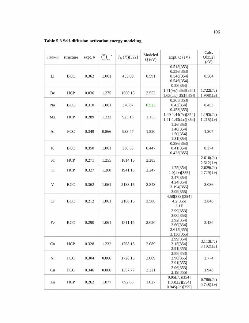
106
Table 5.3 Self-diffusion activation energy modeling.
Element structure expt. 𝜈 (𝑏
𝑠)𝑆𝐷
* 𝑇𝑀(𝐾)[322] Modeled
Q (eV) Expt. Q (eV)
Calc.
Q[352]
(eV)
Li BCC 0.362 1.061 453.69 0.591
0.518[353]
0.556[353]
0.548[354]
0.546[354]
0.58[354]
0.584
Be HCP 0.036 1.275 1560.15 2.553 1.71(//c)[353][354]
1.63(⊥c)[353][354]
1.722(//c)
1.908(⊥c)
Na BCC 0.310 1.061 370.87 0.523
0.365[353]
0.43[354]
0.453[355]
0.453
Mg HCP 0.289 1.232 923.15 1.153 1.40-1.44(//c)[354]
1.41-1.43(⊥c)[354]
1.193(//c)
1.215(⊥c)
Al FCC 0.349 0.866 933.47 1.520
1.26[353]
1.48[354]
1.50[354]
1.31[354]
1.307
K BCC 0.350 1.061 336.53 0.447
0.386[353]
0.41[354]
0.423[355]
0.374
Sc HCP 0.271 1.255 1814.15 2.283 2.610(//c)
2.612(⊥c)
Ti HCP 0.327 1.260 1941.15 2.247 1.75[354]
2.0(⊥c)[355]
2.629(//c)
2.729(⊥c)
V BCC 0.362 1.061 2183.15 2.843
3.47[354]
4.24[354]
3.194[355]
3.09[355]
3.086
Cr BCC 0.212 1.061 2180.15 3.508
4.58[353][354]
4.2[355]
3.1F
3.846
Fe BCC 0.290 1.061 1811.15 2.626
2.99[353]
3.00[353]
2.92[354]
2.60[354]
2.615[355]
3.130[355]
3.136
Co HCP 0.328 1.232 1768.15 2.089
2.99[354]
3.15[354]
2.91[355]
3.113(//c)
3.102(⊥c)
Ni FCC 0.304 0.866 1728.15 3.009
2.88[353]
2.96[355]
2.91[355]
2.774
Cu FCC 0.346 0.866 1357.77 2.221 2.06[353]
2.19[355] 1.948
Zn HCP 0.262 1.077 692.68 1.027
0.95(//c)[354]
1.00(⊥c)[354]
0.945(//c)[355]
0.780(//c)
0.748(⊥c)

107
1.054(⊥c) [355]
Y HCP 0.245 1.274 1799.15 2.309 2.62(//c)[354]
2.91(⊥c)[354]
2.495(//c)
2.521(⊥c)
Zr HCP 0.336 1.255 2128.15 2.437
3.2[353]
1.16-3.64[353]
3.17(//c)[355]
2.605(//c)
2.779(⊥c)
Nb BCC 0.397 1.061 2750.15 3.386 3.62[353]
4.163[355] 3.365
Mo BCC 0.296 1.061 2896.15 4.161 4.53[353]
4.99[355] 4.180
Rh FCC 0.264 0.866 2237.15 4.117 4.05[353] 3.958
Pd FCC 0.385 0.866 1828.05 2.811
2.76[353]
2.76[354]
2.59[355]
2.430
Ag FCC 0.369 0.866 1234.93 1.948
1.76[353]
1.96[355]
1.912[355]
1.76[355]
1.597
Cd HCP 0.344 1.061 594.22 0.796
0.81(//c)[353][354]
0.85(⊥c)[353][354]
0.789(//c)[355]
0.828(⊥c)[355]
0.475(//c)
0.408(⊥c)
Gd HCP 0.261 1.260 1586.15 2.017 1.42[354] 2.161(//c)
2.282 (⊥c)
Tb HCP 0.258 1.265 1629.15 2.068 2.242(//c)
2.334(⊥c)
Dy HCP 0.245 1.271 1685.15 2.169 2.344(//c)
2.414(⊥c)
Ho HCP 0.234 1.274 1747.15 2.274 2.397(//c)
2.452(⊥c)
Er HCP 0.240 1.274 1770.15 2.288 3.13(//c)[354]
3.14(⊥c)[354]
2.498(//c)
2.539(⊥c)
Hf HCP 0.284 1.266 2506.15 3.072
3.84(//c)[354]
3.61(⊥c)[354]
3.345[355]
3.191(//c)
3.364(⊥c)
Ta BCC 0.342 1.061 3290.15 4.421
3.8[353]
4.39[353]
4.13[353]
4.07[353]
4.28[354]
4.39[354]
3.849
W BCC 0.280 1.061 3695.15 5.435
5.45[353]
6.084[355]
6.487[355]
5.210
Re HCP 0.293 1.239 3459.15 4.275 5.3[353] 5.662(//c)
4.915 (⊥c)
Ir FCC 0.250 0.866 2739.15 5.140 4.54[354] 4.639
Ir FCC-s 0.250 0.943 2739.15 4.196 4.54[354] 4.639
Pt FCC 0.396 0.866 2041.45 3.086
2.96[354]
2.89[354]
2.67[355]
2.208

108
Au FCC 0.424 0.866 1337.33 1.926
1.806[354]
1.826[354]
1.810[355]
1.73[355]
1.247
Pb FCC 0.409 0.866 600.61 0.888
1.11[354]
1.05[355]
1.075[355]
1.031
Th FCC 0.287 0.866 2023.15 3.606
3.1-3.32[353]
3.11[354]
3.22[355]
3.469
Th FCC-s 0.287 0.943 2023.15 3.312
3.1-3.32[353]
3.11[354]
3.22[355]
3.469
TiC
[Ti] NaCl 0.218 1.000 3430 5.806 7.649[356]
TiC
[C] NaCl 0.218 1.633 3430 3.556 3.404[314]
ZrC
[Zr] NaCl 0.181 1.000 3805.15 6.752 7.45[357]
ZrC
[C] NaCl 0.181 1.633 3805.15 4.135 3.148[314],a
NbC[N
b] NaCl 0.284 1.000 3763.15 5.836 5.51[357], [358]
NbC
[C] NaCl 0.284 1.633 3763.15 3.574 3.113[314],a
TaC
[C] NaCl 0.230 1.633 4215.15 4.305 3.487[314],a
MgO NaCl 0.188 1.000 3125.15[359
] 5.496
4.258
4.77[360]
AgCl NaCl 0.3590.
420 1.000 728.15
1.011
0.915
1.567[311]
0.736-0.829(𝑄𝐼𝑆𝐷)
[361]
1.02(𝑄𝑉𝑆𝐷) [361]
AgBr NaCl 0.345
0.440 1.000 707.15
1.000
0.858
1.276[311]
0.622-
0.777(𝑄𝐼𝑆𝐷)[361]
0.881(𝑄𝑉𝑆𝐷) [361]
CsCl CsCl 0.222
0.280 1.000 918.15
1.548
1.432
1.561[311]
1.555[361]
KCl NaCl 0.101 1.000 1049.15 2.043 2.096[311]
2.021[361]
KI NaCl 0.061 1.000 959 1.950 1.767[311]
KBr NaCl 0.118 1.000 1003 1.916 2.131[311]
KF NaCl 0.151 1.000 1130 2.078 2.196[311]
LiBr NaCl 0.200 1.000 823.15 1.426 1.347[361]
LiCl NaCl 0.272
0.230 1.000 883.15
1.399
1.473
1.647[311]
1.503[361]
LiF NaCl 0.254
0.210 1.000 1121.15
1.801
1.918
2.196[311]
1.917[361]
LiI NaCl 0.240 1.000 722.15 1.189 0.985[361]
NaCl NaCl 0.164 1.000 1073.15 1.945 2.136[311]

109
0.240 1.766 1.969[361]
NaBr NaCl 0.170 1.000 1028 1.848 2.016[311]
NaF NaCl 0.174 1.000 1261 2.256 2.690[311]
RbCl NaCl 0.131 1.000 988 1.859
1.986 (𝑄𝑉𝑆𝐷) [311]
1.606-2.125(𝑄𝐼𝑆𝐷)
[361]
Si Diamond
Cubic 0.220 0.612 1687.15 4.654
5.141[311]
4.65 (𝑄𝑉𝑆𝐷) [362]
4.82 (𝑄𝐼𝑆𝐷) [362]
4.644[363]
4.77[364]
Ge Diamond
Cubic 0.207 0.612 1211.35 3.396
3.36[311]
3.14[365]
3.05[366]
3.09[367]
GaAs ZnS 0.243 0.612 1511.15 4.045
4.24(𝑄𝐺𝑎𝑆𝐷)[368]
4[369]
4.0[370]
5.6(𝑄𝐺𝑎𝑆𝐷)[371]
InP ZnS 0.276 0.612 1335.15 3.417 3.85(𝑄𝐼𝑛
𝑆𝐷)[372]
5.65(𝑄𝑃𝑆𝐷)[372]
GaSb ZnS 0.227 0.612 985.15 2.692
3.148(𝑄𝐺𝑎𝑆𝐷) [373]
3.443(𝑄𝑆𝑏𝑆𝐷) [373]
1.59(𝑄𝑆𝑏𝑆𝐷)[374]
3.24(𝑄𝐺𝑎𝑆𝐷)[374]
InSb ZnS 0.287 0.612 800.15 2.019
1.813(𝑄𝐼𝑛𝑆𝐷) [373]
1.934(𝑄𝑆𝑏𝑆𝐷) [373]
1.45 (𝑄𝐼𝑛𝑆𝐷) [343]
1.91(𝑄𝑆𝑏𝑆𝐷) [343]
ZnS ZnS 0.291 0.707 1458.15 3.166 3.15[375]
ZnSe ZnS 0.300 0.707 1798.15 3.855 3.0[376]
3.45[377]
ZnTe ZnS 0.301 0.707 1511.15 3.235 2.69[378]
*(𝑏
𝑠)𝑆𝐷 is obtained from Table 5.2.
[ ] diffusion species

110
Chapter 6
Hardness Modeling for Layered Structures: The Origin of Hall-Petch
Relation
6.1 Introduction
The yield (or flow) stress and hardness of polycrystalline materials usually increase as the
grain size (d) decreases from millimeters to tens of nanometers according to the Hall-Petch
relationship[379], [380]. This behavior is mainly due to the dislocations being hindered (pinned)
by grain boundaries[381]. Such dislocation hindering originates from a higher energy barrier at the
grain boundary for dislocations to pass through the boundary than for dislocations to move within
grain. That is to say, as the grains become smaller, the number of piled up dislocations at grain
boundaries increase due to the increase in the density of higher energy barriers; in turn, the effect
of dislocation blocking increases, strengthening materials[382]. The increased yield stress or
hardness is inversely proportional to the square root of grain size as expressed in Equation 6.1 and
Equation 6.2.
Equation 6.1 𝝈 = 𝝈𝟎 + 𝒌𝒅−𝟏
𝟐
Equation 6.2 𝑯𝑽 = 𝑯𝑽,𝟎 + 𝒌𝒅−𝟏
𝟐
Where 𝜎0 and 𝐻𝑉,0 are yield and hardness of the bulk state, k is a Hall-Petch coefficient, and d is
the grain size. Due to the simplicity and well-fitting nature of the equation, Equation 6.1 and
Equation 6.2 are widely used to demonstrate the effect of grain boundary strengthening in pure
metals and alloys[383]–[396]. The coefficient k has been estimated for pure metals and alloys[389].

111
Many attempts have been made to interpret the physical meaning behind the Hall-Petch
relationship by establishing a universal relation for all materials[397]–[405]. Some researchers
modified the original Hall-Petch relation as part of a power law expansion in order to capture the
yield (flow) stress and hardness of different crystal structured pure metals and alloys. Despite their
great efforts, the physical meaning behind this empirical relation has not yet been fully resolved.
To be specific, due to the simplicity of Equation 6.1 and Equation 6.2, these relations do not
consider crystal structures, slip systems, grain misorientations, other slip system activation at grain
boundaries, and other defect structures beyond grain boundaries, etc.
The grain misorientation or grain boundary energy, one of these key factors, plays an
important role in increasing 𝜎 (or 𝐻𝑉) for the same grain size. In the grain size (or twin size)
dependent hardness plot of FCC Cu as shown in Figure 6.1, the hardness values for the same grain
size deviate more than 1 GPa, although the average hardness seems to follow the Hall-Petch relation
trend. In part, this deviation is due to variations in grain misorientation and/or grain boundary
energy since the experimental hardness data of all the twin boundary cases[406]–[408], which has
a lower grain boundary energy, are lower than that of grain size effect[409]–[416]. Thus, the Hall-
Petch relation breaks down, that is, the twin-size dependent hardness, since the Hall-Petch line
should be parabolic to meet the bulk state hardness, 0.362 GPa at 0 (grain size)-1/2. It should be
noted that the grain size dependent hardness experimental data[409]–[416] are mostly from the
ECAP process which results in high angle grain misorientations[417]. Furthermore, Li et al.[418]
showed that hardness increases by increasing the grain misorientation from 2 to 20 degrees in their
dislocation-grain boundary penetration model. Li et al. also pointed out a changing of the Hall-
Petch coefficient (k) due to grain misorientation. Therefore, the grain misorientation or grain
boundary energy plays an important role in determining hardness.

112
0.0 0.1 0.2 0.3 0.4 0.5
1
2
3
4
H
ard
ness (
GP
a)
Grain size-1/2
(nm-1/2
)
Chen et al.(G)
Sanders et al.(G)
Jiang et al.(G)
Agnew et al.(G)
Gray et al.(G)
Valiev et al.(G)
Haouaoui et al.(G)
Suryanarayanan et al.(G)
You et al.(T)
Schwaiger et al.(T)
Anderoglu et al.(T)
0.37
Figure 6.1. Grain size dependent hardness of FCC Cu. Grain size (G) dependent hardness
(solid shapes) are from Chen et al.,[409] Sanders et al.,[410] Jiang et al.,[411] Agnew et
al.,[412] Gray et al.,[413] Valiev et al.,[414] Haouaoui et al.[415], and Suryanarayanan et
al.[416] twin size(T) dependent hardness are from You et al.[406], Lu et al.[407] and
Anderoglu et al.[408].
In addition, other slip systems at the boundary due to the presence of the twin (or grain)
boundaries possibly can be activated depending on the crystal structure. These activated slip
systems near the boundary will increase the energy barrier for dislocations to move, if so, then this
results in dislocation pile-ups near the boundary. For example, it is reported that the 1
2< 110 >
screw dislocations, which are originated from the 1
6[112] partial dislocations near twin boundary
regions in twinned FCC structures, are observed from both experiments and calculations[386],
[419]–[424], although the major slip system for FCC metals are edge dislocations of ½
<110>{111}.
In the present work, in order to systematically investigate the origin of the Hall-Petch
relation from the microscale, twinned FCC Cu, Ag, and carbon diamond structures with various

113
bilayer distances are used since twin boundaries can be considered to be coherent grain boundaries.
For modeling twin-size dependent hardness, the Peierls-Nabarro (PN) flow stress are used since
the PN flow stress equation estimates well the various crystals’ experimental flow stress[15], [425].
To effectively model the slip system angle term, one of the assumptions in classical PN flow stress
is that a dislocation moves through the straight-forward slip direction; this enables to calculate the
flow stress of curved slip direction. Further, additional slip system activation due to the existence
of twin boundaries in FCC metals is also considered. As such, this model will give an idea of how
a curved slip system increases the flow stress and the indentation hardness.
6.2 Methodology
6.2.1 Derivation of Peierls-Nabarro Flow Stress for Twinned Structures
The Peierls-Nabarro (PN) flow stress is the minimum shear stress to overcome the energy
barrier (PN potential) for a dislocation and to move the dislocation. The PN flow stress at 0 K for
edge and screw dislocations are expressed below[15], [235]
Equation 6.3 𝝉𝑷𝑵
𝑮(𝒆𝒅𝒈𝒆) =
𝟏
(𝟏−𝝂)𝒆𝒙𝒑(
−𝟐𝝅𝒘
𝒃)
Equation 6.4 𝝉𝑷𝑵
𝑮(𝒔𝒄𝒓𝒆𝒘) = 𝒆𝒙𝒑(
−𝟐𝝅𝒘
𝒃)
where 𝐺 is shear stress, 𝜈 the Poisson’s ratio, b the Burgers vector and w the dislocation width. The
dislocation width, w, is equal to 𝑠
(1−𝑣) for edge dislocations at 0 K and 𝑠 for screw dislocations[15].
Here, the Burgers vector and the dislocation width are based on full dislocations, i.e., <110> slip
direction on {111} planes for FCC crystals and their derivatives (including diamond cubic)
structures since the PN flow stress equation is for a straight-forward dislocation movement[426],
[427].

114
However, the PN flow stress of twinned structures is more complex since the full
dislocation and the slip planes in twinned structures are not in a straight line and not on a flat slip
plane, but instead they are distorted with certain angles near the twin boundaries as shown in Figure
6.2. Thus, in order to model the angle term in the twinned structures, the angle relationship between
two partial dislocations in FCC and diamond cubic structures are investigated, i.e., 120 for two
1/6<211> Shockley partial dislocations in FCC and 109.47 for two ¼ <111> glide partial
dislocations. Since the PN potential, estimated from these partial dislocations, should be equal to
that estimated from full dislocations, the angle between two partial dislocations plays a crucial role
in determining the PN flow stress. Therefore, the distorted angle should be captured by b/s in
Equation 6.3 and Equation 6.4 as expressed as follows.
Equation 6.5 𝒃𝒇𝒖𝒍𝒍
𝒔𝒇𝒖𝒍𝒍=𝒃𝒑𝒂𝒓𝒕𝒊𝒂𝒍
𝒔𝒑𝒂𝒓𝒕𝒊𝒂𝒍𝒇(𝜽𝒑)
Where 𝜃𝑝 is the angle between two partial dislocation vectors, i.e., 60 for FCC and 70.53 for
diamond cubic structures. The b/s of partial and full dislocations and the angles for FCC and
diamond cubic structures are listed in Table 6.1 and Figure 6.3.
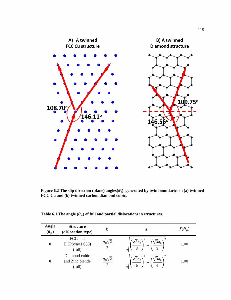
115
Figure 6.2 The slip direction (plane) angles(𝜽𝒊) generated by twin boundaries in (a) twinned
FCC Cu and (b) twinned carbon diamond cubic.
Table 6.1 The angle (𝜽𝒑) of full and partial dislocations in structures.
Angle
(𝜽𝒑)
Structure
(dislocation type) b s 𝒇(𝜽𝒑)
0
FCC and
HCP(c/a=1.633)
(full)
𝑎0√2
2 √(
√3𝑎03)
2
+ (√3𝑎03)
2
1.00
0
Diamond cubic
and Zinc blende
(full)
𝑎0√2
2 √(
√3𝑎06)
2
+ (√3𝑎06)
2
1.00
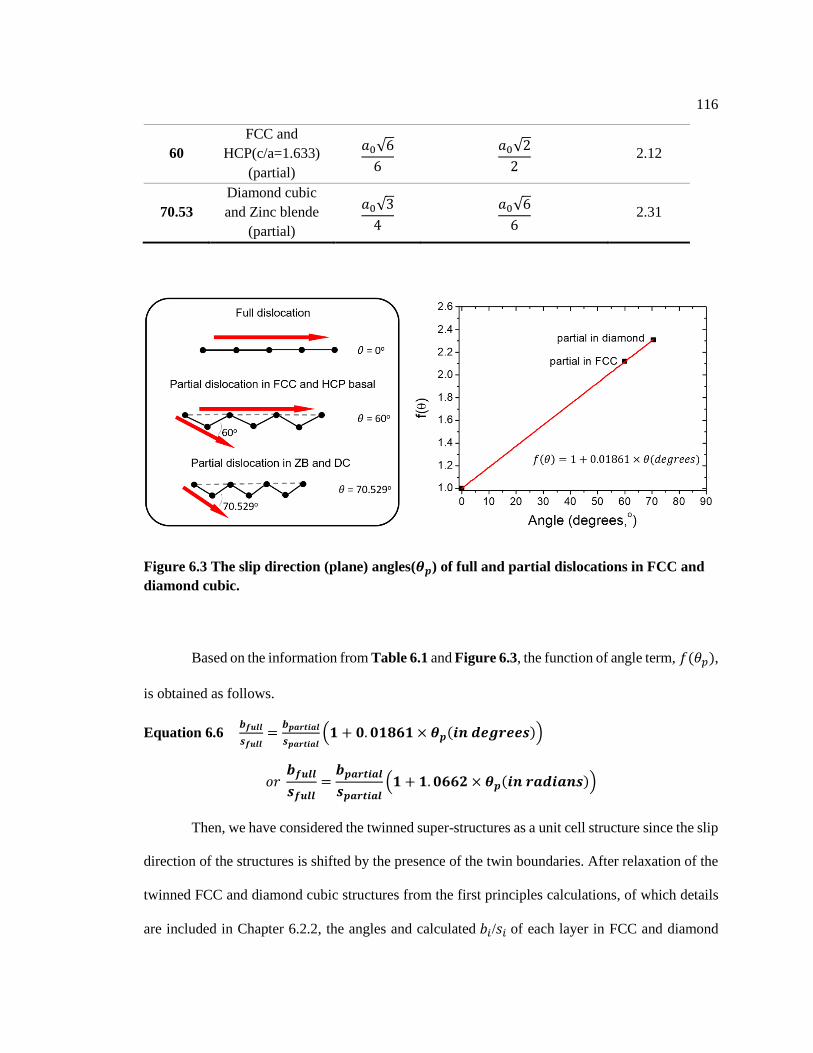
116
60
FCC and
HCP(c/a=1.633)
(partial)
𝑎0√6
6
𝑎0√2
2 2.12
70.53
Diamond cubic
and Zinc blende
(partial)
𝑎0√3
4
𝑎0√6
6 2.31
Figure 6.3 The slip direction (plane) angles(𝜽𝒑) of full and partial dislocations in FCC and
diamond cubic.
Based on the information from Table 6.1 and Figure 6.3, the function of angle term, 𝑓(𝜃𝑝),
is obtained as follows.
Equation 6.6 𝒃𝒇𝒖𝒍𝒍
𝒔𝒇𝒖𝒍𝒍=𝒃𝒑𝒂𝒓𝒕𝒊𝒂𝒍
𝒔𝒑𝒂𝒓𝒕𝒊𝒂𝒍(𝟏 + 𝟎. 𝟎𝟏𝟖𝟔𝟏 × 𝜽𝒑(𝒊𝒏 𝒅𝒆𝒈𝒓𝒆𝒆𝒔))
𝑜𝑟 𝒃𝒇𝒖𝒍𝒍
𝒔𝒇𝒖𝒍𝒍=𝒃𝒑𝒂𝒓𝒕𝒊𝒂𝒍
𝒔𝒑𝒂𝒓𝒕𝒊𝒂𝒍(𝟏 + 𝟏. 𝟎𝟔𝟔𝟐 × 𝜽𝒑(𝒊𝒏 𝒓𝒂𝒅𝒊𝒂𝒏𝒔))
Then, we have considered the twinned super-structures as a unit cell structure since the slip
direction of the structures is shifted by the presence of the twin boundaries. After relaxation of the
twinned FCC and diamond cubic structures from the first principles calculations, of which details
are included in Chapter 6.2.2, the angles and calculated 𝑏𝑖/𝑠𝑖 of each layer in FCC and diamond

117
cubic structures for the three possible slip directions, which move across the twin boundary, are
obtained as shown in Figure 6.4 based on Equation 6.6. Then, the 𝑏𝑖/𝑠𝑖 of each layer is averaged
by a root mean square (RMS) averaging scheme as shown in Figure 6.5 since the slip system
modulation are similar to that of the electric current. The three possible slip directions in twinned
diamond cubic and FCC structures towards twin boundaries are averaged by arithmetic mean of
three possible slip directions. Therefore, the twin boundary bilayer based bsd
ssd term is obtained as
follows.
Equation 6.7 𝐛𝐬𝐝
𝐬𝐬𝐝= √
𝟏
𝐧∑ (
𝐛𝐢
𝐬𝐢𝐟(𝛉𝐢))
𝟐
𝐧𝐢
Where n is the number of layers between twin boundaries and 𝑖 is the 𝑖th layer, bsd and ssd are
Burgers vector and slip plane spacing for the superdislocation, respectively.
Figure 6.4 Normalized 𝒃𝒊/𝒔𝒊 (with respect to that of each structures) changes of each layers
in (a) twinned carbon diamond cubic and (b) FCC Cu.

118
Figure 6.5 Schematics of the method of modeling of b/s in twinned structures.
By putting Equation 6.7 into Equation 6.3, the flow stress of twinned structure was obtained
as follows.
Equation 6.8 𝝉𝑷𝑵
𝑮(𝒆𝒅𝒈𝒆) =
𝟏
(𝟏−𝝂)𝐞𝐱𝐩 (
−𝟐𝝅
(𝟏−𝝂)
𝐬𝐬𝐝
𝐛𝐬𝐝)
Furthermore, the modeled hardness was calculated by integrating Equation 6.8 into the
hardness model proposed in Chapter 4 and Chapter 5 as follows. The modeled hardness is room
temperature based, see Chapter 5 for detailed information.
Equation 6.9 𝑯𝒗 = 𝟎. 𝟏𝟔𝟏𝟓 𝑮 (𝟏 + 𝟐𝟖𝟓𝟕. 𝟏𝒘𝐬𝐝
𝐛𝐬𝐝(𝐛𝐬𝐝
𝐬𝐬𝐝)𝟐(𝝉𝑷𝑵
𝑮)𝟐)𝟐
𝒆−𝟐.𝟐𝒌 (𝐛𝐬𝐝
𝐬𝐬𝐝)𝟒𝐭𝐚𝐧𝟑/𝟐 𝒂 𝐜𝐨𝐬𝒂
Where k is the Pugh ratio which is shear modulus over bulk modulus (G/B) and 𝑎 is the indenter
angle which is 22 .

119
6.2.2 First-Principles Calculations
First-principles calculations are performed using the Vienna Ab-initio Simulation Package
(VASP)[27], [28], [31]. Electron-ion interactions are described by the projector augmented-wave
(PAW) method[29], and the X-C functionals depicted by the generalized gradient approximation
(GGA), as implemented by Perdew, Burke, and Ernzerhof (PBE)[30], are used. The plane wave
cutoff energy of 520 (C), 390 (Cu) and 360 (Ag) eV is used for all calculations; this is 1.3 times of
the recommended values by VASP[31]. For primitive diamonds and face centered cubic structures
and their twinned structures, more than 8000 k-points are implemented. The k-mesh guarantees
errors below 0.1meV/atom. The structures are relaxed by the Methfessel-Paxton method[76]. After
relaxations, a final static calculation using the tetrahedral method with Blöch corrections[36] is
applied to ensure the accuracy of total energy. The crystal structures of diamond carbons, Cu and
Ag are considered to be diamond cubic (Fd3m) and face centered cubic (Fm3m) structures, and the
twinned structures of both diamond cubic and FCC used in this study are sigma 3 boundaries on
(111) plane.
In the present work, elastic stiffness constants are predicted at 0 K via the stress–strain
method from first-principles calculations[39]. The detailed descriptions are the same as the
calculation of elastic stiffness constants of LPSO in Chapter 2.2
6.3 Results and Discussion
In the present twin bilayer dependent hardness model, the local active slip system 𝑏𝑖/𝑠𝑖
changes due to the presence of twin boundaries in FCC and diamond cubic structures are
investigated. The active slip system, 𝑏 = ½ < 110 >, of the twinned structure is not straight-
forward but curved near the twin boundaries as shown in Figure 6.2, Figure 6.4 and Figure 6.5,
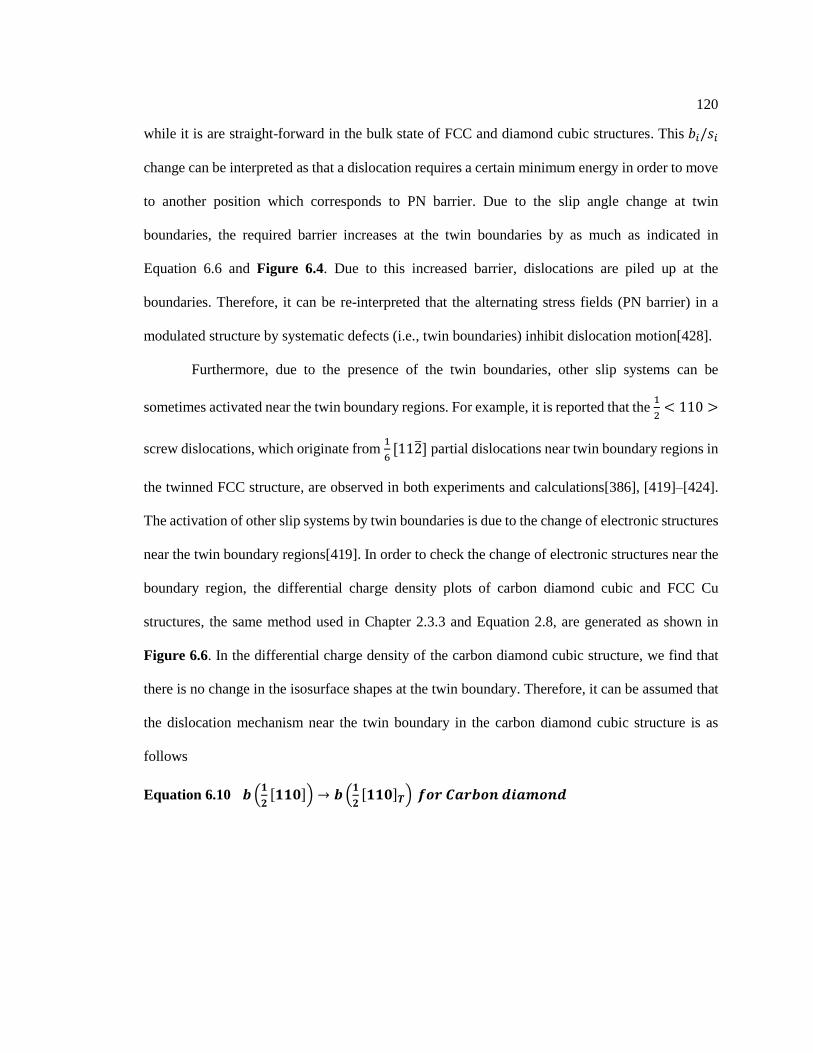
120
while it is are straight-forward in the bulk state of FCC and diamond cubic structures. This 𝑏𝑖/𝑠𝑖
change can be interpreted as that a dislocation requires a certain minimum energy in order to move
to another position which corresponds to PN barrier. Due to the slip angle change at twin
boundaries, the required barrier increases at the twin boundaries by as much as indicated in
Equation 6.6 and Figure 6.4. Due to this increased barrier, dislocations are piled up at the
boundaries. Therefore, it can be re-interpreted that the alternating stress fields (PN barrier) in a
modulated structure by systematic defects (i.e., twin boundaries) inhibit dislocation motion[428].
Furthermore, due to the presence of the twin boundaries, other slip systems can be
sometimes activated near the twin boundary regions. For example, it is reported that the 1
2< 110 >
screw dislocations, which originate from 1
6[112] partial dislocations near twin boundary regions in
the twinned FCC structure, are observed in both experiments and calculations[386], [419]–[424].
The activation of other slip systems by twin boundaries is due to the change of electronic structures
near the twin boundary regions[419]. In order to check the change of electronic structures near the
boundary region, the differential charge density plots of carbon diamond cubic and FCC Cu
structures, the same method used in Chapter 2.3.3 and Equation 2.8, are generated as shown in
Figure 6.6. In the differential charge density of the carbon diamond cubic structure, we find that
there is no change in the isosurface shapes at the twin boundary. Therefore, it can be assumed that
the dislocation mechanism near the twin boundary in the carbon diamond cubic structure is as
follows
Equation 6.10 𝒃 (𝟏
𝟐[𝟏𝟏𝟎]) → 𝒃(
𝟏
𝟐[𝟏𝟏𝟎]𝑻) 𝒇𝒐𝒓 𝑪𝒂𝒓𝒃𝒐𝒏 𝒅𝒊𝒂𝒎𝒐𝒏𝒅

121
Figure 6.6 Differential charge density plots of (a) carbon diamond cubic (reference state),
(b) FCC Cu (reference state), (c) twinned carbon diamond cubic and (d) twinned FCC Cu
structures. Red arrows indicate the close-up view of twin boundary area. Isosurfaces are
0.0065 (e/Å 3) and the atom sizes are exaggerated for better visualization.
However, we found the change of the isosurface shape in twinned FCC Cu from a
tetragonal (triangle in 2 Dimension) to a prism (rectangular in 2D) near the twin boundaries. This
indicates that the active slip system near the regions is probably not the same as that of the bulk
state, which is expected to be 𝟏
𝟐[𝟏𝟏𝟎] . Based on previous research on possible dislocation
mechanisms near twin boundaries for FCC metals,[386], [419]–[424] the Shockley partial

122
dislocations (𝟏
𝟔[𝟏𝟏��]) are activated near twin boundaries,[419] and these partial dislocation pairs
mostly have combined screw characteristics instead of edge characteristic [386] as expressed in
Equation 6.11. The active slip system is originated from the electronic structure, i.e., the
unsaturated d-bonds[131]. Therefore, it is assumed that the region where the partial or screw
dislocations are activated is limited to two layers away from the twin boundary as shown in Figure
6.6.
Equation 6.11 𝒃 (𝟏
𝟐[𝟏𝟏𝟎]) → 𝒃𝟏 (
𝟏
𝟐[𝟏𝟏𝟎]𝑻) + 𝒃𝟐 (
𝟏
𝟔[𝟏𝟏��] ) 𝒇𝒐𝒓 𝑭𝑪𝑪 𝒎𝒆𝒕𝒂𝒍𝒔
Based on Equation 6.10 for carbon diamond cubic and Equation 6.11 for FCC Cu, we have
calculated b/s as shown in Figure 6.4. Interestingly, 𝐛𝐢
𝐬𝐢 for carbon diamond cubic at the twin
boundary increases up to 2.3 times of that of the bulk state, while that for FCC Cu at the twin
boundary increases up to 11 times of that of the bulk state due to the activation of screw
dislocations. After averaging 𝐛𝐢
𝐬𝐢 based on the methodology as shown in Figure 6.5 and expressed
in Equation 6.7, 𝐛𝐬𝐝
𝐬𝐬𝐝 of the relaxed twinned structures with different twin bilayer distances are
calculated as shown in Figure 6.7. It should be noted that the relative change of 𝐛𝐬𝐝
𝐬𝐬𝐝 in the carbon
diamond cubic structure for a 10 nm twin bilayer increases 2.7% with respect to that of the bulk
state, while that in FCC Cu for a 10 nm twin bilayer increases 84.2% from that of the bulk state
due to the activation of partial dislocations near the twin boundaries.
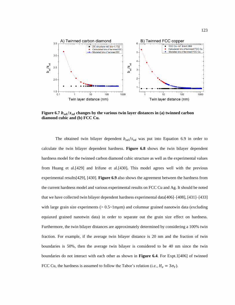
123
Figure 6.7 𝒃𝒔𝒅/𝒔𝒔𝒅 changes by the various twin layer distances in (a) twinned carbon
diamond cubic and (b) FCC Cu.
The obtained twin bilayer dependent 𝑏𝑠𝑑/𝑠𝑠𝑑 was put into Equation 6.9 in order to
calculate the twin bilayer dependent hardness. Figure 6.8 shows the twin bilayer dependent
hardness model for the twinned carbon diamond cubic structure as well as the experimental values
from Huang et al.[429] and Irifune et al.[430]. This model agrees well with the previous
experimental results[429], [430]. Figure 6.9 also shows the agreement between the hardness from
the current hardness model and various experimental results on FCC Cu and Ag. It should be noted
that we have collected twin bilayer dependent hardness experimental data[406]–[408], [431]–[433]
with large grain size experiments (> 0.5~1m𝜇m) and columnar grained nanotwin data (excluding
equiaxed grained nanotwin data) in order to separate out the grain size effect on hardness.
Furthermore, the twin bilayer distances are approximately determined by considering a 100% twin
fraction. For example, if the average twin bilayer distance is 20 nm and the fraction of twin
boundaries is 50%, then the average twin bilayer is considered to be 40 nm since the twin
boundaries do not interact with each other as shown in Figure 6.4. For Expt.1[406] of twinned
FCC Cu, the hardness is assumed to follow the Tabor’s relation (i.e., 𝐻𝑣 = 3𝜎𝑌).

124
Figure 6.8 Hardness of diamond carbon as a function of twin bilayer distance. Expt.1 and 2
are from Huang et al.[429] and Irifune et al.[430], respectively. Open blue triangles are
obtained from relaxed structures calculated from first-principles calculations.
Figure 6.9 Hardness of FCC (a) Cu and (b) Ag as a function of twin bilayer distance. For (a)
FCC Cu, Expt.1 from You et al.[406], Expt.2 from Lu et al.[407] and Expt.3 from
Anderoglu et al.[408] are included. For (b) FCC Ag, Expt.1 from Bufford et al.[431], Expt.2
from Bufford et al.[432] and Expt.3 from Furnish et al.[433] are included. Red dash line is
the hardness of their bulk state.
In order to compare the hardness model with the Hall-Petch relation, Figure 6.10 shows
the hardness as a function of (twin bilayer)-1/2 of twinned carbon diamond, FCC Cu and FCC Ag.
This also shows that the classical Hall-Petch relation breaks down especially for carbon diamonds.
The experimental hardness of a twinned carbon diamond in Figure 6.10 clearly shows that the

125
experimental data do not follow the linear Hall-Petch relation from the point of (0,100) which is
the hardness of the bulk state, but the hardness trend of the experiment data follows this model. For
FCC metals, although the trend is not stronger than that of carbon diamond since it is very difficult
to separate out twin bilayer effect on hardness, the hardness trend does not follow the Hall-Petch
relation (i.e., the linear line in Figure 6.10). However, the experimental hardness trend is captured
by this model.

126
Figure 6.10 Hall-Petch relationship in hardness of (a) carbon diamond, (b) FCC Cu and (c)
FCC Ag as a function of twin bilayer distance. References are from those in Figure 6.8 and
Figure 6.9. ★ in the plots are the hardness of bulk state, and these are from Teter[215] for
carbon diamond, from Samsonov[291] for FCC Cu and Ag. Red dash lines are the slope for
Hall-Petch relation.

127
Chapter 7
Hardness Modeling of LPSO Phases
In this chapter, the hardness models developed in Chapter 4, Chapter 5 and Chapter 6 are
applied to LPSO phases in order to predict the hardness of LPSO phases in the Mg-Al-Gd system.
This chapter mainly focuses on the prediction of the hardness of LPSO phases in the Mg-Al-Gd
system by the determination of the factors that affect the hardness, also discussed in previous
chapters.
7.1 Methodology
Based on the hardness models presented in Chapter 4, Chapter 5, and Chapter 6, the
chemical composition contribution (i.e., diluted phases such as Cu-2at.%Ni) on hardness are
captured by the elastic properties (shear and bulk moduli) and the change of the active slip systems
(the mechanical paths how the dislocations move in the crystal lattice). The slip systems are
distorted near the defects, i.e., vacancies, impurity atoms and twin boundaries, and the slip systems
are no longer the same as that without defects.
In order to predict the hardness of any material, the following information is needed: (1)
active slip systems, (2) melting temperature and (3) elastic properties (described in Chapter 4), (4)
diffusion mechanisms (described in Chapter 5), and (5) slip system angle term and additional slip
system activation if the slip systems are not straight-forward (described in Chapter 6).
For the prediction of the hardness of LPSO phases, the melting temperature is obtained
from Figure 3.9 in Chapter 3, and elastic properties of LPSO phases used in this study are from
Table 2.3. The diffusion mechanisms of LPSO phases are assumed to be the same as that of HCP
Mg since slip occurs along the weakest bonds, which are between mg layers on basal plane or move

128
between L12 clusters surrounded by Mg atoms. In order to determine active slip systems of LPSO
phases, we first determine the LPSO structures, (Mg)116(Gd)16(Al)12(Gd)2 for 18R and
(Mg)140(Gd)16(Al)12(Mg)2 for 14H, based on their phase stability discussed in Chapter 3. For the
active slip systems of LPSO phases, basal slip on {0001} for 14H and 18R LPSOs, pyramidal slip
on {1108} for 18R and prismatic slip on {1100}for 14H are considered based on Hagihara et
al.[434] as shown in Figure 7.1. The slip system angle terms for LPSO phases are calculated using
Equation 6.6 as discussed in Chapter 6.
Figure 7.1 Slip systems of (a) 18R and (b) 14H LPSOs. Thin solid lines are the pyramidal
slip, black thick lines are the slip direction within FCC layers, red thick lines are the basal
slip, and dash lines are the L12 cluster.
7.2 Results and Discussion
Since the values of indentation hardness and flow stress change exponentially as the change
of b/s (slip system term), the determinations of the 𝑏𝑖/𝑠𝑖 of 14H and 18R LPSO structures are
crucial to predict hardness. Although the basal slip systems of both 14H and 18R LPSOs are simply

129
obtained since they are straight-forward, the pyramidal slips are calculated based on the 𝑏𝑖/𝑠𝑖 of
14H and 18R LPSO structures as shown in Figure 7.2.
Figure 7.2 𝒃𝒊/𝒔𝒊 changes of (a) 18R and (b) 14H LPSOs. Pyramidal slip on {1��08} for 18R
and prismatic slip on {1��00} for 14H are applied.
As there are no hardness data for LPSO phases in the Mg-Al-Gd systems, we instead used
the hardness data for LPSO phases in the Mg-Zn-Y systems[435]–[440] since the elastic properties
of both Mg-Al-Gd and Mg-Zn-Y are very similar (less than 8% difference in shear modulus, see
Table 2.3) and the atomic displacements in Mg layers are negligible.
Based on the hardness models and the above information, the predicted hardness of 18R
and 14H LPSO phases in the Mg-Al-Gd system is 1.81 GPa (18R) and 1.38 GPa (14H) for
pyramidal slip and 0.87 GPa (18R) 0.86 GPa (14H) for basal slip. Since the proposed hardness
model considers individual slip systems due to the lack of the slip system ratio information, and
also the indentation hardness measurement is orientation dependent property that affects the ratio
of the active slip systems, the predicted LPSOs’ hardness would rather give the ranges of the
hardness based on individual slip systems such as basal and pyramidal slips. For example, the
model with basal slip is the minimum hardness and that with pyramidal slip is the maximum
hardness. This trend agrees well with the experimental values from literatures[435]–[440] as shown

130
in Figure 7.3. Furthermore, the hardness of LPSO phases is 2.5 (basal) to 6 (pyramidal) times larger
for 18R and 2.5(basal) to 4.5 (pyramidal) times larger for 14H than that of HCP Mg[291].
Figure 7.3 Hardness prediction of 18R and 14H LPSO phases. Expt. 1 to Expt. 6 are from
[435] (Expt. 1), [49] (Expt. 2), [437] (Expt. 3), [438] (Expt. 4), [439] (Expt. 5), [440] (Expt. 6),
and the hardness of polycrystalline Mg as a reference[291] (Expt. 7), respectively.

131
Chapter 8
Conclusions and Future Work
8.1 Conclusions
Chapter 2 investigates the effects of L12 clusters and interstitial atoms (Mg, Gd, and Al)
on the structural and elastic properties of the Mg-Gd-Al LPSO phases via first-principles
calculations. Key conclusions can be summarized as follows:
(i) The number of layers in the SB affects the cluster densities along [0001] direction,
and this results in the changes of C33 and E[0001].
(ii) The size of L12 clusters is a key lattice feature to determine the C11 and C66.
(iii) For a SB with the same number of fault layers, an L12 cluster with an interstitial
atom in the LPSO increases the bulk modulus, Young’s modulus, and shear
modulus.
(iv) Effects of the number of fault layers in SB on elastic properties, such as bulk
modulus, are traceable to the redistribution of differential charge densities caused
by alloying elements.
In Chapter 3, thermodynamic properties of the 10H, 14H, 18R, and 24R LPSO phases in
the Mg-Al-Gd ternary system are predicted by first-principles calculations and modeled via the
CALPHAD method. The LPSO phases are modelled by four sublattices to capture the L12 cluster
embedded in the FCC stacking layers, including the atomic occupancy in the center interstitial site
within the cluster. Thermodynamic properties of the LPSO endmembers are obtained through the
quasiharmonic phonon and Debye models from first-principles calculations. It is observed that the
pure Mg endmembers of the LPSO phases are less stable with respect to HCP Mg; the occupancy

132
of the interstitial site by atoms are energetically favorable; and the mixing in the interstitial site is
nearly ideal. The presently thermodynamic description of the LPSO phases reproduces well the
phase equilibria reported in the literature, for example, the 18R is stable at high temperatures, the
14H is stable at low temperatures, and the 10H and 24R phases are not stable in the Mg-Ga-Al
system.
In Chapter 4, a new hardness model applicable to both ductile/brittle materials is developed
through the consideration of both elastic and plastic deformations of materials for the first time. It
incorporates the Peierls-Nabarro flow stress, dislocation width, Burgers vector, and slip plane
spacing in addition to the shear and bulk moduli. The model is based on the fundamental
understanding of elastic and plastic deformations during the indentation experiment, and the two
model parameters which are evaluated from the ratio of total and plastic indentation depths and the
experimental hardness values reported in the literature. In addition to hardness, the present model
can give insights on the possible dominant active slip systems by comparing the predicted hardness
values of various slip systems. The present hardness model provides a long-missing capability in
quantitatively predicting the mechanical properties of materials and future development of
ultrahard materials.
In Chapter 5, the unified temperature dependent hardness model for Vickers hardness is
proposed based on the dislocation width as a function of temperature. The dislocation width is truly
affected by the materials’ deformation diffusion mechanisms which include dislocation diffusion
and self-diffusion. This temperature dependent hardness model will help to predict materials
hardness as a function of temperature as well as other mechanical properties such as flow stress.
This model will accelerate materials design for mechanical properties as a function of temperature.
In Chapter 6, the twin bilayer dependent Vickers hardness model is proposed based on the
dislocation width as a function of twin bilayer. The dislocation width is affected by the twin
boundaries. Importantly the presence of the twin boundaries will accelerate the activation of the
133
screw dislocations in FCC metals which is generated from the partial dislocation of 1
6[112]. This
twin bilayer dependent hardness model will help to predict materials hardness as a function of twin
bilayer as well as other mechanical properties such as flow stress. This model will accelerate
materials design for mechanical properties.
In Chapter 7, the Vickers hardness models developed by Chapter 4, Chapter 5 and Chapter
6 are applied to 18R and 14H LPSO phases in Mg-Al-Gd system. Basal slip and pyramidal slip are
applied to this hardness model for LPSO phases. This model agrees well with various experimental
results.
8.2 Future Work
(1) Determination of the active slip systems in various crystal structures from first-
principles calculations.
(2) Modeling hardness as a function of the grain size by taking considerations of grain
misorientation angles and other slip system mechanisms.
(3) Modeling of LPSO hardness as a function of temperature by calculations of
diffusion activation energies.

134
Appendix A
Complete Elastic Stiffness Matrixes of 10H, 18R and 24R LPSO Phases
Type System Int. C11 C22 C33 C12 C13 C23 C44 C55 C66 C15 C25 C35 C46 B G E 𝜈 Ref.
10H
Mg-Gd-Al no 74.9 76.4 87.4 27.7 17.6 17.4 24.8 23.7 22.4 0 0 0 0 40.8 25.4 63.1 0.239 This work
Mg-Gd-Al Al 79.9 80.3 91.6 28.9 17.5 17.6 25.2 25.1 26.0 0 0 0 0 42.1 27.5 67.8 0.230 This work
Mg-Gd-Al Mg 78.8 79.0 90.4 28.8 17.5 17.5 23.7 23.8 24.6 0 0 0 0 41.9 26.3 65.2 0.237 This work
Mg-Gd-Al Gd 75.6 75.3 86.8 29.5 19.4 18.8 24.1 23.7 19.7 0 0 0 0 42.2 23.9 60.4 0.256 This work
18R
Mg-Gd-Al no 72.8 73.8 84.3 27.6 16.9 13.7 23.8 26.7 22.0 3.8 -4.1 0.6 -1.2 38.8 25.5 62.8 0.226 This work
Mg-Gd-Al Al 78.0 79.5 89.0 26.7 18.9 17.2 26.0 27.0 25.1 1.9 -2.6 0.8 -2.2 41.6 27.5 67.6 0.227 This work
Mg-Gd-Al Mg 77.1 78.1 88.9 27.2 18.5 17.1 26.3 27.4 23.8 3.3 -4.4 1.6 -2.1 41.4 27.1 66.8 0.228 This work
Mg-Gd-Al Gd 76.0 75.7 87.9 25.4 18.3 25.7 23.7 25.1 22.0 3.0 -5.1 1.1 -1.3 41.3 25.3 62.9 0.242 This work
Mg-Y-Zn no 70.4 70.4 85.3 30.1 19.8 19.0 21.7 24.1 20.0 -3.3 2.1 0.9 1.5 40.5 23.2 58.5 0.256 This work
Mg-Y-Zn Zn 70.5 69.1 84.6 32.4 18.5 20.4 20.3 23.3 19.4 -4.0 2.7 1.1 4.1 40.6 22.5 56.9 0.263 This work
Mg-Y-Zn Mg 71.6 69.6 85.4 32.3 17.9 20.3 21.7 24.2 20.2 -3.8 3.2 1.2 4.1 40.6 23.4 58.9 0.256 This work
Mg-Y-Zn Y 71.6 69.7 84.3 30.4 19.5 19.9 22.6 23.1 18.4 -2.2 -0.4 2.0 3.9 41.0 22.5 57.1 0.263 This work
Mg-Y-Zn 72.5
±0.7
80.0
±1.8 -
18.9
±1.1
23.5
±0.3
21.2
±0.3 - -
73.0 ±1.9 58.4 ±0.3
Exp. [26]
no 71.6 70.6 82.0 28.7 19.7 19.6 23.2 22.9 21.1 -2.5 2.3 0.5 1.7 Calc. [26]

135
Zn 72.3 73.4 84.2 28.8 18.8 18.8 24.2 24.2 21.5 -3.4 3.2 -0.1 2.6 Calc. [26]
Mg 71.9 72.7 85.2 29.1 18.8 18.7 24.8 24.7 21.8 -3.8 3.5 0.1 2.6 Calc. [26]
Y 72.7 73.2 83.8 28.1 19.4 18.9 24.6 24.3 22.1 -3.4 3.3 0.3 2.0 Calc. [26]
Mg-Y-Zn - - - - - - - - 66.7 ±4.9
Exp. [49]
Mg-Y-Zn 67.7 ±1.0
72.9 ±2.0
28.3 ±1.1
19.5 ±0.8
21.5 ±0.3
19.7 ±0.3
38.0 ±0.7
65.0 ±1.4 54.0 ±0.6
Exp. RT
[53]
Mg-Y-Zn 68.1 ±1.0
67.2 ±0.9
21.6 ±0.7
24.0 ±0.8
20.6 ±0.2
23.2 ±0.2
- 21.8 ±0.1
54.9 ±0.4
Exp. RT
[53] Mg-Y-Zn no 71.6 70.6 82.0 28.7 19.7 19.6 23.2 22.9 21.1 -2.5 2.3 0.5 1.7 Calc. [53]
24R
Mg-Gd-Al no 73.1 73.1 82.9 24.5 16.1 15.3 24.9 24.3 21.3 2.8 -2.5 0.2 -1.3 38.5 24.9 61.5 0.229 This work
Mg-Gd-Al Al 77.7 77.0 85.1 25.5 17.1 18.1 25.1 25.3 25.0 1.9 -1.5 -0.2 -1.1 40.4 26.7 65.6 0.227 This work
Mg-Gd-Al Mg 76.2 74.6 85.7 27.4 15.5 18.8 26.0 27.1 24.0 3.1 -2.8 -0.1 -0.5 40.0 26.8 65.8 0.224 This work
Mg-Gd-Al Gd 74.1 71.7 86.6 28.8 15.4 18.9 27.8 28.5 20.4 2.8 -1.2 -1.7 -0.5 40.2 25.9 63.9 0.230 This work

136
Appendix B
Thermo-Calc Mg-Al-Gd Database
$ *********************
$ File name: MgGdAlwithLPSOphases.TDB
$ *********************
$-----------------------------------------------------------------------------
$ Thermodynamic database of the Mg-Gd-Al system, modeled by Hongyeun Kim
$ + Phases Research Lab
$ Department of Materials Science and Engineering
$ The Pennsylvania State University
$ Last update: May 20, 2018
$-----------------------------------------------------------------------------
$ the model parameters of LPSO phases are mole-formula based
$ while those in the manuscript are mole-atom based
$
ELEMENT /- ELECTRON_GAS 0.0000E+00 0.0000E+00 0.0000E+00!
ELEMENT VA VACUUM 0.0000E+00 0.0000E+00 0.0000E+00!
ELEMENT AL FCC_A1 2.6982E+01 4.5773E+03 2.8322E+01!
ELEMENT GD HCP_A3 1.5725E+02 0.0000E+00 0.0000E+00!

137
ELEMENT MG HCP_A3 2.4305E+01 4.9980E+03 3.2671E+01!
FUNCTION GHSERAL 298.15 -7976.15+137.093038*T-24.3671976*T*LN(T)
-.001884662*T**2-8.77664E-07*T**3+74092*T**(-1); 700 Y
-11276.24+223.048446*T-38.5844296*T*LN(T)+.018531982*T**2
-5.764227E-06*T**3+74092*T**(-1); 933.47 Y
-11278.378+188.684153*T-31.748192*T*LN(T)-1.230524E+28*T**(-9); 2900 N
!
FUNCTION GHSERGD 200 -6834.5855+97.13101*T-24.7214131*T*LN(T)
-.00285240521*T**2-3.14674076E-07*T**3-8665.73348*T**(-1); 1000 Y
-6483.25362+95.6919924*T-24.6598297*T*LN(T)-.00185225011*T**2
-6.61211607E-07*T**3; 1508.15 Y
-123124.992+699.125537*T-101.800197*T*LN(T)+.0150644246*T**2
-6.39165948E-07*T**3+29356890.3*T**(-1); 3600 N !
FUNCTION GHSERMG 298.15 -8367.34+143.677875*T-26.1849782*T*LN(T)
+4.858E-04*T**2-1.393669E-06*T**3+78950*T**(-1); 923 Y
-14130.185+204.718543*T-34.3088*T*LN(T)+1.038192E+28*T**(-9); 3000 N !
FUNCTION GA12GDMG 298.15 -50000+50*T; 3000 N !
FUNCTION GA12MGAL 298.15 +97875-101.5*T; 3000 N !
FUNCTION GA12MG 298.15 +133469-87.319*T; 3000 N !
FUNCTION GA12ALMG 298.15 -52780-50.75*T; 3000 N !
FUNCTION GALBCC 298.15 +10083-4.813*T+GHSERAL#; 6000 N !
FUNCTION GGDFCC 298.15 +1800-.1*R#*T+GHSERGD#; 3600 N !
FUNCTION GALLAV 298.15 +15000+3*GHSERAL#; 3000 N !

138
FUNCTION GGDLAV 298.15 +15000+3*GHSERGD#; 3000 N !
FUNCTION GC15ALGD 298.15 -160000+32.64*T; 3000 N !
FUNCTION GC15GDMG 298.15 -45000+9.972*T; 3000 N !
FUNCTION GMGLAV 298.15 +15000+3*GHSERMG#; 3000 N !
FUNCTION GC36ALGD 298.15 +GC15ALGD#+13000; 3000 N !
FUNCTION GC36GDMG 298.15 +GC15GDMG#+15000; 3000 N !
FUNCTION GALLIQ 298.15 +3028.879+125.251171*T-24.3671976*T*LN(T)
-.001884662*T**2-8.77664E-07*T**3+74092*T**(-1)+7.9337E-20*T**7; 700 Y
-271.21+211.206579*T-38.5844296*T*LN(T)+.018531982*T**2
-5.764227E-06*T**3+74092*T**(-1)+7.9337E-20*T**7; 933.47 Y
-795.996+177.430178*T-31.748192*T*LN(T); 2900 N !
FUNCTION GGDLIQ 100 +6225.4407+88.8092103*T-24.7214131*T*LN(T)
-.00285240521*T**2-3.14674076E-07*T**3-8665.73348*T**(-1); 1000 Y
+146262.037-1208.70685*T+159.352082*T*LN(T)-.108247135*T**2
+1.06945505E-05*T**3-19678357*T**(-1); 1508.15 Y
-5397.314+192.336215*T-38.5075*T*LN(T); 3600 N !
FUNCTION GMGLIQ 298.15 +8202.24-8.83693*T-8.01759E-20*T**7+GHSERMG#; 923
Y
+8690.32-9.39216*T-1.03819E+28*T**(-9)+GHSERMG#; 6000 N !
FUNCTION UN_ASS 298.15 +0.0; 300 N !
TYPE_DEFINITION % SEQ *!
DEFINE_SYSTEM_DEFAULT ELEMENT 2 !
DEFAULT_COMMAND DEF_SYS_ELEMENT VA /- !

139
PHASE AL2GD3 % 2 2 3 !
CONSTITUENT AL2GD3 :AL : GD : !
PARAMETER G(AL2GD3,AL:GD;0) 298.15 -220000+55.89*T+2*GHSERAL#
+3*GHSERGD#; 3000 N REF0 !
PHASE AL3GD % 2 3 1 !
CONSTITUENT AL3GD :AL : GD : !
PARAMETER G(AL3GD,AL:GD;0) 298.15 -165000+29.61*T+3*GHSERAL#
+GHSERGD#; 3000 N REF0 !
PHASE ALGD % 2 1 1 !
CONSTITUENT ALGD :AL : GD : !
PARAMETER G(ALGD,AL:GD;0) 298.15 -98000+23*T+GHSERAL#
+GHSERGD#; 3000 N REF0 !
PHASE ALGD2 % 2 1 2 !
CONSTITUENT ALGD2 :AL : GD : !

140
PARAMETER G(ALGD2,AL:GD;0) 298.15 -115500+30.4*T+GHSERAL#
+2*GHSERGD#; 3000 N REF0 !
PHASE ALMG_BETA % 2 140 89 !
CONSTITUENT ALMG_BETA :AL : MG : !
PARAMETER G(ALMG_BETA,AL:MG;0) 298.15 -803385+105.238*T
+140*GHSERAL#+89*GHSERMG#; 6000 N REF0 !
PHASE ALMG_EPSILON % 2 30 23 !
CONSTITUENT ALMG_EPSILON :AL : MG : !
PARAMETER G(ALMG_EPSILON,AL:MG;0) 298.15 -170832-8.047*T+30*GHSERAL#
+23*GHSERMG#; 6000 N REF0 !
PHASE ALMG_GAMMA % 3 5 12 12 !
CONSTITUENT ALMG_GAMMA :GD,MG : AL,MG : AL,MG : !
PARAMETER G(ALMG_GAMMA,GD:AL:AL;0) 298.15 +GA12GDMG#+GA12MGAL#
-GA12MG#; 3000 N REF0 !
PARAMETER G(ALMG_GAMMA,MG:AL:AL;0) 298.15 +8360+20.338857*T
+5*GHSERMG#+24*GHSERAL#; 6000 N REF0 !

141
PARAMETER G(ALMG_GAMMA,GD:MG:AL;0) 298.15 +GA12GDMG#-GA12MG#
+GA12ALMG#; 3000 N REF0 !
PARAMETER G(ALMG_GAMMA,MG:MG:AL;0) 298.15 -104308.83+23.495281*T
+17*GHSERMG#+12*GHSERAL#; 6000 N REF0 !
PARAMETER G(ALMG_GAMMA,GD:AL:MG;0) 298.15 +GA12GDMG#+GA12MGAL#
-GA12ALMG#; 3000 N REF0 !
PARAMETER G(ALMG_GAMMA,MG:AL:MG;0) 298.15 +180556-138.069*T
+17*GHSERMG#+12*GHSERAL#; 6000 N REF0 !
PARAMETER G(ALMG_GAMMA,GD:MG:MG;0) 298.15 +GA12GDMG#; 3000 N
REF0 !
PARAMETER G(ALMG_GAMMA,MG:MG:MG;0) 298.15 +139371-87.319*T
+29*GHSERMG#; 6000 N REF0 !
PARAMETER G(ALMG_GAMMA,MG:AL:AL,MG;0) 298.15 +113100-14.5*T; 6000 N
REF0 !
PARAMETER G(ALMG_GAMMA,MG:MG:AL,MG;0) 298.15 +113100-14.5*T; 6000 N
REF0 !
TYPE_DEFINITION & GES A_P_D BCC_A2 MAGNETIC -1.0 4.00000E-01 !
PHASE BCC_A2 %& 2 1 3 !
CONSTITUENT BCC_A2 :AL,GD,MG : VA : !
PARAMETER G(BCC_A2,AL:VA;0) 298.15 +GALBCC#; 3000 N REF0 !
PARAMETER G(BCC_A2,GD:VA;0) 100 -3600.77684+95.0191641*T
-24.7214131*T*LN(T)-.00285240521*T**2-3.14674076E-07*T**3

142
-8665.73348*T**(-1); 1000 Y
+152792.743-1349.58873*T+180.097094*T*LN(T)-.119550229*T**2
+1.17915728E-05*T**3-22038836*T**(-1); 1508.15 Y
-15783.7618+202.222057*T-38.960425*T*LN(T); 1586.15 Y
-19850.5562+224.817909*T-41.904333*T*LN(T)+8.58222759E-04*T**2
-3.77570269E-08*T**3+995428.573*T**(-1); 3600 N REF0 !
PARAMETER G(BCC_A2,MG:VA;0) 298.14 -5267.34+141.575547*T
-26.1849782*T*LN(T)+4.858E-04*T**2-1.393669E-06*T**3+78950*T**(-1); 923 Y
-11030.185+202.616215*T-34.3088*T*LN(T)+1.038192E+28*T**(-9); 3000 N REF0 !
PARAMETER G(BCC_A2,AL,GD:VA;0) 298.15 -80000+30.64*T; 6000 N REF0 !
PARAMETER G(BCC_A2,GD,MG:VA;0) 298.15 -45347.5+25.5692*T; 6000 N
REF0 !
PARAMETER G(BCC_A2,GD,MG:VA;1) 298.15 +10195+1.3355*T; 6000 N
REF0 !
PARAMETER G(BCC_A2,GD,MG:VA;2) 298.15 +3267.1-3.5551*T; 6000 N
REF0 !
PHASE FCC_A1 % 2 1 1 !
CONSTITUENT FCC_A1 :AL,GD,MG : VA : !
PARAMETER G(FCC_A1,AL:VA;0) 298.15 +GHSERAL#; 3000 N REF0 !
PARAMETER G(FCC_A1,GD:VA;0) 298.15 +GGDFCC#; 3000 N REF0 !
PARAMETER G(FCC_A1,MG:VA;0) 298.15 +2600-.9*T+GHSERMG#; 3000 N
REF0 !

143
PARAMETER G(FCC_A1,AL,MG:VA;0) 298.15 +1593+2.149*T; 6000 N REF0 !
PARAMETER G(FCC_A1,AL,MG:VA;1) 298.15 +1014-.66*T; 6000 N REF0 !
PARAMETER G(FCC_A1,AL,MG:VA;2) 298.15 -673; 6000 N REF0 !
PHASE GDMG3 % 2 1 3 !
CONSTITUENT GDMG3 :GD : MG : !
PARAMETER G(GDMG3,GD:MG;0) 298.15 -57000+13.0162*T+3*GHSERMG#
+GHSERGD#; 3000 N REF0 !
PHASE GDMG5 % 2 1 5 !
CONSTITUENT GDMG5 :GD : MG : !
PARAMETER G(GDMG5,GD:MG;0) 298.15 -60521.6+11.2668*T
+5*GHSERMG#+GHSERGD#; 3000 N REF0 !
TYPE_DEFINITION ' GES A_P_D HCP_A3 MAGNETIC -3.0 2.80000E-01 !
PHASE HCP_A3 %' 2 1 .5 !
CONSTITUENT HCP_A3 :AL,GD,MG : VA : !
PARAMETER G(HCP_A3,AL:VA;0) 298.15 +5481-1.8*T+GHSERAL#; 3000
N REF0 !
144
PARAMETER TC(HCP_A3,GD:VA;0) 200 +293.4; 3600 N REF0 !
PARAMETER BMAGN(HCP_A3,GD:VA;0) 200 +3; 3600 N REF0 !
PARAMETER G(HCP_A3,GD:VA;0) 298.15 +GHSERGD#; 3000 N REF0 !
PARAMETER G(HCP_A3,MG:VA;0) 298.15 +GHSERMG#; 3000 N REF0 !
PARAMETER G(HCP_A3,AL,MG:VA;0) 298.15 +4336-2.863*T; 6000 N REF0 !
PARAMETER G(HCP_A3,AL,MG:VA;1) 298.15 -449-.135*T; 6000 N REF0 !
PARAMETER G(HCP_A3,AL,MG:VA;2) 298.15 -1963; 6000 N REF0 !
PARAMETER G(HCP_A3,GD,MG:VA;0) 298.15 -33346.6+19.3451*T; 6000 N
REF0 !
PARAMETER G(HCP_A3,GD,MG:VA;1) 298.15 +13854; 6000 N REF0 !
PHASE LAV_C14 % 2 1 2 !
CONSTITUENT LAV_C14 :AL,GD : AL,GD : !
PARAMETER G(LAV_C14,AL:AL;0) 298.15 +GALLAV#; 3000 N REF0 !
PARA G(LAV_C14,GD:AL;0) 298.15 +0; 6000 N!
PARA G(LAV_C14,AL:GD;0) 298.15 +0; 6000 N!
PARAMETER G(LAV_C14,GD:GD;0) 298.15 +GGDLAV#; 3000 N REF0 !
PHASE LAV_C15 % 2 1 2 !
CONSTITUENT LAV_C15 :AL,GD,MG : AL,GD,MG : !
PARAMETER G(LAV_C15,AL:AL;0) 298.15 +GALLAV#; 3000 N REF0 !

145
PARAMETER G(LAV_C15,GD:AL;0) 298.15 +GC15ALGD#+2*GHSERAL#
+GHSERGD#; 3000 N REF0 !
PARAMETER G(LAV_C15,MG:AL;0) 298.15 +15000+2*GHSERAL#+GHSERMG#;
3000 N REF0 !
PARAMETER G(LAV_C15,AL:GD;0) 298.15 -GC15ALGD#+30000+GHSERAL#
+2*GHSERGD#; 3000 N REF0 !
PARAMETER G(LAV_C15,GD:GD;0) 298.15 +GGDLAV#; 3000 N REF0 !
PARAMETER G(LAV_C15,MG:GD;0) 298.15 -GC15GDMG#+32000+2*GHSERGD#
+GHSERMG#; 3000 N REF0 !
PARAMETER G(LAV_C15,AL:MG;0) 298.15 +15000+GHSERAL#+2*GHSERMG#;
3000 N REF0 !
PARAMETER G(LAV_C15,GD:MG;0) 298.15 -50777+17.149*T+2*GHSERMG#
+GHSERGD#; 3000 N REF0 !
PARAMETER G(LAV_C15,MG:MG;0) 298.15 +GMGLAV#; 3000 N REF0 !
PARAMETER G(LAV_C15,GD:AL,MG;0) 298.15 +29500; 3000 N REF0 !
PARAMETER G(LAV_C15,GD:AL,MG;1) 298.15 -10000; 3000 N REF0 !
PHASE LAV_C36 % 2 1 2 !
CONSTITUENT LAV_C36 :AL,GD,MG : AL,GD,MG : !
PARAMETER G(LAV_C36,AL:AL;0) 298.15 +GALLAV#; 3000 N REF0 !
PARAMETER G(LAV_C36,GD:AL;0) 298.15 +GC36ALGD#+2*GHSERAL#
+GHSERGD#; 3000 N REF0 !
PARAMETER G(LAV_C36,MG:AL;0) 298.15 -500+2*GHSERAL#+GHSERMG#;

146
3000 N REF0 !
PARAMETER G(LAV_C36,AL:GD;0) 298.15 -GC36ALGD#+30000+GHSERAL#
+2*GHSERGD#; 3000 N REF0 !
PARAMETER G(LAV_C36,GD:GD;0) 298.15 +GGDLAV#; 3000 N REF0 !
PARAMETER G(LAV_C36,MG:GD;0) 298.15 -GC36GDMG#+30000+2*GHSERGD#
+GHSERMG#; 3000 N REF0 !
PARAMETER G(LAV_C36,AL:MG;0) 298.15 +30500+GHSERAL#+2*GHSERMG#;
3000 N REF0 !
PARAMETER G(LAV_C36,GD:MG;0) 298.15 +GC36GDMG#+GHSERGD#
+2*GHSERMG#; 3000 N REF0 !
PARAMETER G(LAV_C36,MG:MG;0) 298.15 +GMGLAV#; 3000 N REF0 !
PARAMETER G(LAV_C36,GD,MG:AL;0) 298.15 -45000+9*T; 3000 N REF0 !
PHASE LIQUID % 1 1.0 !
CONSTITUENT LIQUID :AL,GD,MG : !
PARAMETER G(LIQUID,AL;0) 298.15 +GALLIQ#; 3000 N REF0 !
PARAMETER G(LIQUID,GD;0) 298.15 +GGDLIQ#; 3000 N REF0 !
PARAMETER G(LIQUID,MG;0) 298.15 +GMGLIQ#; 3000 N REF0 !
PARAMETER G(LIQUID,AL,GD;0) 298.15 -166500+52.36*T; 6000 N
REF0 !
PARAMETER G(LIQUID,AL,GD;1) 298.15 -23790; 6000 N REF0 !
PARAMETER G(LIQUID,AL,GD;2) 298.15 +18520; 6000 N REF0 !
PARAMETER G(LIQUID,AL,GD,MG;0) 298.15 -20000; 6000 N REF0 !

147
PARAMETER G(LIQUID,AL,MG;0) 298.15 -9019+4.794*T; 6000 N REF0 !
PARAMETER G(LIQUID,AL,MG;1) 298.15 -1093+1.412*T; 6000 N REF0 !
PARAMETER G(LIQUID,AL,MG;2) 298.15 +494; 6000 N REF0 !
PARAMETER G(LIQUID,GD,MG;0) 298.15 -36681.3+16.2484*T; 6000 N
REF0 !
PARAMETER G(LIQUID,GD,MG;1) 298.15 +34233.8-10.7783*T; 6000 N
REF0 !
PARAMETER G(LIQUID,GD,MG;2) 298.15 -7352.9; 6000 N REF0 !
PHASE LPSO10H % 4 92 16 12 2 !
CONSTITUENT LPSO10H :MG : AL,GD,MG : AL,GD,MG : AL,GD,MG,VA : !
PARA G(LPSO10H,MG:AL:AL:AL;0) 298.15 +0; 6000 N!
PARAMETER G(LPSO10H,MG:GD:AL:AL;0) 298.15 -2354532.08+16774.99*T
-3070.98*T*LN(T)-.2397*T**2+9194000*T**(-1)-3.106E-05*T**3;
3000 N REF0 !
PARA G(LPSO10H,MG:MG:AL:AL;0) 298.15 +0; 6000 N!
PARA G(LPSO10H,MG:AL:GD:AL;0) 298.15 +0; 6000 N!
PARA G(LPSO10H,MG:GD:GD:AL;0) 298.15 +0; 6000 N!
PARA G(LPSO10H,MG:MG:GD:AL;0) 298.15 +0; 6000 N!
PARA G(LPSO10H,MG:AL:MG:AL;0) 298.15 +0; 6000 N!
PARA G(LPSO10H,MG:GD:MG:AL;0) 298.15 +0; 6000 N!
PARA G(LPSO10H,MG:MG:MG:AL;0) 298.15 +0; 6000 N!
PARA G(LPSO10H,MG:AL:AL:GD;0) 298.15 +0; 6000 N!

148
PARAMETER G(LPSO10H,MG:GD:AL:GD;0) 298.15 -2365966.81+16331.7*T
-3055.52*T*LN(T)-.2668*T**2+7265000*T**(-1)-2.528E-05*T**3;
3000 N REF0 !
PARA G(LPSO10H,MG:MG:AL:GD;0) 298.15 +0; 6000 N!
PARA G(LPSO10H,MG:AL:GD:GD;0) 298.15 +0; 6000 N!
PARA G(LPSO10H,MG:GD:GD:GD;0) 298.15 +0; 6000 N!
PARA G(LPSO10H,MG:MG:GD:GD;0) 298.15 +0; 6000 N!
PARA G(LPSO10H,MG:AL:MG:GD;0) 298.15 +0; 6000 N!
PARA G(LPSO10H,MG:GD:MG:GD;0) 298.15 +0; 6000 N!
PARA G(LPSO10H,MG:MG:MG:GD;0) 298.15 +0; 6000 N!
PARA G(LPSO10H,MG:AL:AL:MG;0) 298.15 +0; 6000 N!
PARAMETER G(LPSO10H,MG:GD:AL:MG;0) 298.15 -2360302.63+16684.48*T
-3065.66*T*LN(T)-.2439*T**2+8772000*T**(-1)-2.815E-05*T**3;
3000 N REF0 !
PARA G(LPSO10H,MG:MG:AL:MG;0) 298.15 +0; 6000 N!
PARA G(LPSO10H,MG:AL:GD:MG;0) 298.15 +0; 6000 N!
PARA G(LPSO10H,MG:GD:GD:MG;0) 298.15 +0; 6000 N!
PARA G(LPSO10H,MG:MG:GD:MG;0) 298.15 +0; 6000 N!
PARA G(LPSO10H,MG:AL:MG:MG;0) 298.15 +0; 6000 N!
PARA G(LPSO10H,MG:GD:MG:MG;0) 298.15 +0; 6000 N!
PARA G(LPSO10H,MG:MG:MG:MG;0) 298.15 +0; 6000 N!
PARAMETER G(LPSO10H,MG:AL:AL:VA;0) 298.15 -782715.93+17456.09*T
-3061.63*T*LN(T)-.2279*T**2+12980000*T**(-1)-6.045E-05*T**3; 3000 N
REF0 !
PARAMETER G(LPSO10H,MG:GD:AL:VA;0) 298.15 -1955859.12+17048.53*T

149
-3026.71*T*LN(T)-.2572*T**2+12450000*T**(-1)-3.906E-05*T**3;
3000 N REF0 !
PARAMETER G(LPSO10H,MG:MG:AL:VA;0) 298.15 -877620.27+18263.01*T
-3063.8*T*LN(T)-.2318*T**2+6751000*T**(-1)-4.928E-05*T**3; 3000 N
REF0 !
PARAMETER G(LPSO10H,MG:AL:GD:VA;0) 298.15 -1194764.44+15633.3*T
-3031.19*T*LN(T)-.2458*T**2+4779000*T**(-1)-3.293E-05*T**3;
3000 N REF0 !
PARAMETER G(LPSO10H,MG:GD:GD:VA;0) 298.15 -1087653.56+15437.85*T
-3025.65*T*LN(T)-.2935*T**2+4279000*T**(-1)-3.703E-05*T**3; 3000 N
REF0 !
PARAMETER G(LPSO10H,MG:MG:GD:VA;0) 298.15 -910956.4+17993.29*T
-3021.13*T*LN(T)-.2888*T**2+3392000*T**(-1)-3.015E-05*T**3; 3000 N
REF0 !
PARAMETER G(LPSO10H,MG:AL:MG:VA;0) 298.15 -923009.74+16979.14*T
-3027.52*T*LN(T)-.2475*T**2+10570000*T**(-1)-4.14E-05*T**3; 3000 N
REF0 !
PARAMETER G(LPSO10H,MG:GD:MG:VA;0) 298.15 -1337554.87+15898.4*T
-3002.15*T*LN(T)-.2862*T**2+5720000*T**(-1)-2.227E-05*T**3; 3000 N
REF0 !
PARAMETER G(LPSO10H,MG:MG:MG:VA;0) 298.15 -1067584.41+19470.57*T
-3516.43*T*LN(T)+.612039*T**2+15152000*T**(-1)-2.483E-04*T**3; 3000
N REF0 !
PARAMETER G(LPSO10H,MG:AL,GD:AL:VA;0) 298.15 -136647; 3000 N REF0 !
PARAMETER G(LPSO10H,MG:AL,GD:AL:VA;1) 298.15 +671235; 3000 N REF0 !
150
PARAMETER G(LPSO10H,MG:AL,MG:AL:VA;0) 298.15 -2177; 3000 N REF0 !
PARAMETER G(LPSO10H,MG:AL,MG:AL:VA;1) 298.15 +111307; 3000 N REF0 !
PARAMETER G(LPSO10H,MG:AL:AL,GD:VA;0) 298.15 -24208; 3000 N REF0 !
PARAMETER G(LPSO10H,MG:AL:AL,GD:VA;1) 298.15 -912856; 3000 N REF0 !
PARAMETER G(LPSO10H,MG:AL:AL,MG:VA;0) 298.15 -2825; 3000 N REF0 !
PARAMETER G(LPSO10H,MG:AL:AL,MG:VA;1) 298.15 +6782; 3000 N REF0 !
PARAMETER G(LPSO10H,MG:GD,MG:AL:VA;0) 298.15 +154409; 3000 N REF0 !
PARAMETER G(LPSO10H,MG:GD,MG:AL:VA;1) 298.15 +191805; 3000 N REF0 !
PARAMETER G(LPSO10H,MG:GD:AL,GD:VA;0) 298.15 +1095340; 3000 N REF0 !
PARAMETER G(LPSO10H,MG:GD:AL,GD:VA;1) 298.15 -670940; 3000 N REF0 !
PARAMETER G(LPSO10H,MG:GD:AL,MG:VA;0) 298.15 +859085; 3000 N REF0 !
PARAMETER G(LPSO10H,MG:GD:AL,MG:VA;1) 298.15 -725095; 3000 N REF0 !
PARAMETER G(LPSO10H,MG:MG:AL,GD:VA;0) 298.15 +78596; 3000 N REF0 !
PARAMETER G(LPSO10H,MG:MG:AL,GD:VA;1) 298.15 -626763; 3000 N REF0 !
PARAMETER G(LPSO10H,MG:MG:AL,MG:VA;0) 298.15 -14320; 3000 N REF0 !
PARAMETER G(LPSO10H,MG:MG:AL,MG:VA;1) 298.15 -46645; 3000 N REF0 !
PARAMETER G(LPSO10H,MG:AL,GD:GD:VA;0) 298.15 -49024; 3000 N REF0 !
PARAMETER G(LPSO10H,MG:AL,GD:GD:VA;1) 298.15 +259459; 3000 N REF0 !
PARAMETER G(LPSO10H,MG:AL,MG:GD:VA;0) 298.15 +56565; 3000 N REF0 !
PARAMETER G(LPSO10H,MG:AL,MG:GD:VA;1) 298.15 +12235; 3000 N REF0 !
PARAMETER G(LPSO10H,MG:AL:GD,MG:VA;0) 298.15 +35675; 3000 N REF0 !
PARAMETER G(LPSO10H,MG:AL:GD,MG:VA;1) 298.15 -436853; 3000 N REF0 !
PARAMETER G(LPSO10H,MG:GD,MG:GD:VA;0) 298.15 +172246; 3000 N REF0 !
PARAMETER G(LPSO10H,MG:GD,MG:GD:VA;1) 298.15 +81486; 3000 N REF0 !
PARAMETER G(LPSO10H,MG:GD:GD,MG:VA;0) 298.15 -163698; 3000 N REF0 !
151
PARAMETER G(LPSO10H,MG:GD:GD,MG:VA;1) 298.15 +83590; 3000 N REF0 !
PARAMETER G(LPSO10H,MG:MG:GD,MG:VA;0) 298.15 -75509; 3000 N REF0 !
PARAMETER G(LPSO10H,MG:MG:GD,MG:VA;1) 298.15 -181093; 3000 N REF0 !
PARAMETER G(LPSO10H,MG:AL,GD:MG:VA;0) 298.15 -68913; 3000 N REF0 !
PARAMETER G(LPSO10H,MG:AL,GD:MG:VA;1) 298.15 +654423; 3000 N REF0 !
PARAMETER G(LPSO10H,MG:AL,MG:MG:VA;0) 298.15 -30388; 3000 N REF0 !
PARAMETER G(LPSO10H,MG:AL,MG:MG:VA;1) 298.15 +41340; 3000 N REF0 !
PARAMETER G(LPSO10H,MG:GD,MG:MG:VA;0) 298.15 -101085; 3000 N REF0 !
PARAMETER G(LPSO10H,MG:GD,MG:MG:VA;1) 298.15 +243856; 3000 N REF0 !
PHASE LPSO14H % 4 140 16 12 2 !
CONSTITUENT LPSO14H :MG : AL,GD,MG : AL,GD,MG : AL,GD,MG,VA : !
PARA G(LPSO14H,MG:AL:AL:AL;0) 298.15 +0; 6000 N!
PARAMETER G(LPSO14H,MG:GD:AL:AL;0) 298.15 -2786149.21+23028.16*T
-4275.39*T*LN(T)-.3339*T**2+13680000*T**(-1)-4.94E-05*T**3;
3000 N REF0 !
PARA G(LPSO14H,MG:MG:AL:AL;0) 298.15 +0; 6000 N!
PARA G(LPSO14H,MG:AL:GD:AL;0) 298.15 +0; 6000 N!
PARA G(LPSO14H,MG:GD:GD:AL;0) 298.15 +0; 6000 N!
PARA G(LPSO14H,MG:MG:GD:AL;0) 298.15 +0; 6000 N!
PARA G(LPSO14H,MG:AL:MG:AL;0) 298.15 +0; 6000 N!
PARAMETER G(LPSO14H,MG:GD:MG:AL;0) 298.15 -1793340.98+22721.72*T
-4268.55*T*LN(T)-.3833*T**2+11510000*T**(-1)-4.049E-05*T**3; 6000 N REF0 !

152
PARA G(LPSO14H,MG:MG:MG:AL;0) 298.15 +0; 6000 N!
PARA G(LPSO14H,MG:AL:AL:GD;0) 298.15 +0; 6000 N!
PARAMETER G(LPSO14H,MG:GD:AL:GD;0) 298.15 -2813548.65+22801.14*T
-4276.6*T*LN(T)-.3373*T**2+12620000*T**(-1)-4.709E-05*T**3;
3000 N REF0 !
PARA G(LPSO14H,MG:MG:AL:GD;0) 298.15 +0; 6000 N!
PARA G(LPSO14H,MG:AL:GD:GD;0) 298.15 +0; 6000 N!
PARA G(LPSO14H,MG:GD:GD:GD;0) 298.15 +0; 6000 N!
PARA G(LPSO14H,MG:MG:GD:GD;0) 298.15 +0; 6000 N!
PARA G(LPSO14H,MG:AL:MG:GD;0) 298.15 +0; 6000 N!
PARAMETER G(LPSO14H,MG:GD:MG:GD;0) 298.15 -1630377.48+22568*T
-4273.96*T*LN(T)-.3773*T**2+10830000*T**(-1)-3.994E-05*T**3; 6000 N REF0 !
PARA G(LPSO14H,MG:MG:MG:GD;0) 298.15 +0; 6000 N!
PARA G(LPSO14H,MG:AL:AL:MG;0) 298.15 +0; 6000 N!
PARAMETER G(LPSO14H,MG:GD:AL:MG;0) 298.15 -2799969.07+22945.45*T
-4277.98*T*LN(T)-.3293*T**2+13190000*T**(-1)-4.828E-05*T**3;
3000 N REF0 !
PARA G(LPSO14H,MG:MG:AL:MG;0) 298.15 +0; 6000 N!
PARA G(LPSO14H,MG:AL:GD:MG;0) 298.15 +0; 6000 N!
PARA G(LPSO14H,MG:GD:GD:MG;0) 298.15 +0; 6000 N!
PARA G(LPSO14H,MG:MG:GD:MG;0) 298.15 +0; 6000 N!
PARA G(LPSO14H,MG:AL:MG:MG;0) 298.15 +0; 6000 N!
PARAMETER G(LPSO14H,MG:GD:MG:MG;0) 298.15 -1741000.25+22702.32*T
-4274.51*T*LN(T)-.379*T**2+11310000*T**(-1)-4.046E-05*T**3; 6000 N REF0 !
PARA G(LPSO14H,MG:MG:MG:MG;0) 298.15 +0; 6000 N!

153
PARAMETER G(LPSO14H,MG:AL:AL:VA;0) 298.15 -1155694.45+24155.39*T
-4279.5*T*LN(T)-.3259*T**2+18370000*T**(-1)-7.698E-05*T**3; 3000 N
REF0 !
PARAMETER G(LPSO14H,MG:GD:AL:VA;0) 298.15 -2420244.24+22742.55*T
-4234.51*T*LN(T)-.3454*T**2+13370000*T**(-1)-5.397E-05*T**3;
3000 N REF0 !
PARAMETER G(LPSO14H,MG:MG:AL:VA;0) 298.15 -1262380.29+23455.24*T
-4275.57*T*LN(T)-.3317*T**2+14180000*T**(-1)-6.633E-05*T**3; 3000 N
REF0 !
PARAMETER G(LPSO14H,MG:AL:GD:VA;0) 298.15 -1616730.58+22587.99*T
-4252.14*T*LN(T)-.3323*T**2+11050000*T**(-1)-5.01E-05*T**3; 3000 N
REF0 !
PARAMETER G(LPSO14H,MG:GD:GD:VA;0) 298.15 -1410515.73+21426.21*T
-4201.07*T*LN(T)-.4069*T**2+8064000*T**(-1)-3.667E-05*T**3; 3000 N
REF0 !
PARAMETER G(LPSO14H,MG:MG:GD:VA;0) 298.15 -1340489.73+22148.91*T
-4244.11*T*LN(T)-.3631*T**2+9456000*T**(-1)-4.961E-05*T**3; 3000 N
REF0 !
PARAMETER G(LPSO14H,MG:AL:MG:VA;0) 298.15 -1307892.46+23724.09*T
-4239.32*T*LN(T)-.3504*T**2+16650000*T**(-1)-5.953E-05*T**3; 3000 N
REF0 !
PARAMETER G(LPSO14H,MG:GD:MG:VA;0) 298.15 -1711823.78+22404.3*T
-4230.22*T*LN(T)-.3693*T**2+10930000*T**(-1)-4.105E-05*T**3; 3000 N
REF0 !
PARAMETER G(LPSO14H,MG:MG:MG:VA;0) 298.15 -1475214.62+26504.93*T
154
-4796.04*T*LN(T)+.670536*T**2+19341800*T**(-1)-3.04561E-04*T**3;
3000 N REF0 !
PARAMETER G(LPSO14H,MG:AL,GD:AL:VA;0) 298.15 +123091; 3000 N REF0 !
PARAMETER G(LPSO14H,MG:AL,GD:AL:VA;1) 298.15 +754417; 3000 N REF0 !
PARAMETER G(LPSO14H,MG:AL,MG:AL:VA;0) 298.15 +211429; 3000 N REF0 !
PARAMETER G(LPSO14H,MG:AL,MG:AL:VA;1) 298.15 -71145; 3000 N REF0 !
PARAMETER G(LPSO14H,MG:AL:AL,GD:VA;0) 298.15 +120491; 3000 N REF0 !
PARAMETER G(LPSO14H,MG:AL:AL,GD:VA;1) 298.15 -997608; 3000 N REF0 !
PARAMETER G(LPSO14H,MG:AL:AL,MG:VA;0) 298.15 +100358; 3000 N REF0 !
PARAMETER G(LPSO14H,MG:AL:AL,MG:VA;1) 298.15 -116095; 3000 N REF0 !
PARAMETER G(LPSO14H,MG:GD,MG:AL:VA;0) 298.15 -342208; 3000 N REF0 !
PARAMETER G(LPSO14H,MG:GD,MG:AL:VA;1) 298.15 +583484; 3000 N REF0 !
PARAMETER G(LPSO14H,MG:GD:AL,GD:VA;0) 298.15 +836065; 3000 N REF0 !
PARAMETER G(LPSO14H,MG:GD:AL,GD:VA;1) 298.15 -509455; 3000 N REF0 !
PARAMETER G(LPSO14H,MG:GD:AL,MG:VA;0) 298.15 +621910; 3000 N REF0 !
PARAMETER G(LPSO14H,MG:GD:AL,MG:VA;1) 298.15 -540640; 3000 N REF0 !
PARAMETER G(LPSO14H,MG:MG:AL,GD:VA;0) 298.15 +93659; 3000 N REF0 !
PARAMETER G(LPSO14H,MG:MG:AL,GD:VA;1) 298.15 -678979; 3000 N REF0 !
PARAMETER G(LPSO14H,MG:MG:AL,MG:VA;0) 298.15 -5754; 3000 N REF0 !
PARAMETER G(LPSO14H,MG:MG:AL,MG:VA;1) 298.15 -65837; 3000 N REF0 !
PARAMETER G(LPSO14H,MG:AL,GD:GD:VA;0) 298.15 +27178; 3000 N REF0 !
PARAMETER G(LPSO14H,MG:AL,GD:GD:VA;1) 298.15 +200656; 3000 N REF0 !
PARAMETER G(LPSO14H,MG:AL,MG:GD:VA;0) 298.15 +41584; 3000 N REF0 !
PARAMETER G(LPSO14H,MG:AL,MG:GD:VA;1) 298.15 -45712; 3000 N REF0 !
PARAMETER G(LPSO14H,MG:AL:GD,MG:VA;0) 298.15 +34281; 3000 N REF0 !

155
PARAMETER G(LPSO14H,MG:AL:GD,MG:VA;1) 298.15 -450286; 3000 N REF0 !
PARAMETER G(LPSO14H,MG:GD,MG:GD:VA;0) 298.15 -13145; 3000 N REF0 !
PARAMETER G(LPSO14H,MG:GD,MG:GD:VA;1) 298.15 +56621; 3000 N REF0 !
PARAMETER G(LPSO14H,MG:GD:GD,MG:VA;0) 298.15 -234097; 3000 N REF0 !
PARAMETER G(LPSO14H,MG:GD:GD,MG:VA;1) 298.15 -6258; 3000 N REF0 !
PARAMETER G(LPSO14H,MG:MG:GD,MG:VA;0) 298.15 -22621; 3000 N REF0 !
PARAMETER G(LPSO14H,MG:MG:GD,MG:VA;1) 298.15 -164212; 3000 N REF0 !
PARAMETER G(LPSO14H,MG:AL,GD:MG:VA;0) 298.15 -166652; 3000 N REF0 !
PARAMETER G(LPSO14H,MG:AL,GD:MG:VA;1) 298.15 +473551; 3000 N REF0 !
PARAMETER G(LPSO14H,MG:AL,MG:MG:VA;0) 298.15 -13587; 3000 N REF0 !
PARAMETER G(LPSO14H,MG:AL,MG:MG:VA;1) 298.15 +19826; 3000 N REF0 !
PARAMETER G(LPSO14H,MG:GD,MG:MG:VA;0) 298.15 +31690; 3000 N REF0 !
PARAMETER G(LPSO14H,MG:GD,MG:MG:VA;1) 298.15 +142429; 3000 N REF0 !
PHASE LPSO18R % 4 116 16 12 2 !
CONSTITUENT LPSO18R :MG : AL,GD,MG : AL,GD,MG : AL,GD,MG,VA : !
PARA G(LPSO18R,MG:AL:AL:AL;0) 298.15 +0; 6000 N!
PARAMETER G(LPSO18R,MG:GD:AL:AL;0) 298.15 -2586985.99+19691.21*T
-3673.73*T*LN(T)-.2831*T**2+11520000*T**(-1)-4.11E-05*T**3;
3000 N REF0 !
PARA G(LPSO18R,MG:MG:AL:AL;0) 298.15 +0; 6000 N!
PARA G(LPSO18R,MG:AL:GD:AL;0) 298.15 +0; 6000 N!
PARA G(LPSO18R,MG:GD:GD:AL;0) 298.15 +0; 6000 N!
156
PARA G(LPSO18R,MG:MG:GD:AL;0) 298.15 +0; 6000 N!
PARA G(LPSO18R,MG:AL:MG:AL;0) 298.15 +0; 6000 N!
PARAMETER G(LPSO18R,MG:GD:MG:AL;0) 298.15 +0; 6000 N REF0 !
PARA G(LPSO18R,MG:MG:MG:AL;0) 298.15 +0; 6000 N!
PARA G(LPSO18R,MG:AL:AL:GD;0) 298.15 +0; 6000 N!
PARAMETER G(LPSO18R,MG:GD:AL:GD;0) 298.15 -2608111.07+19592.82*T
-3698.42253*T*LN(T)-.2755*T**2+10790000*T**(-1)-4.403E-05*T**3
; 3000 N REF0 !
PARA G(LPSO18R,MG:MG:AL:GD;0) 298.15 +0; 6000 N!
PARA G(LPSO18R,MG:AL:GD:GD;0) 298.15 +0; 6000 N!
PARA G(LPSO18R,MG:GD:GD:GD;0) 298.15 +0; 6000 N!
PARA G(LPSO18R,MG:MG:GD:GD;0) 298.15 +0; 6000 N!
PARA G(LPSO18R,MG:AL:MG:GD;0) 298.15 +0; 6000 N!
PARAMETER G(LPSO18R,MG:GD:MG:GD;0) 298.15 +0; 6000 N REF0 !
PARA G(LPSO18R,MG:MG:MG:GD;0) 298.15 +0; 6000 N!
PARA G(LPSO18R,MG:AL:AL:MG;0) 298.15 +0; 6000 N!
PARAMETER G(LPSO18R,MG:GD:AL:MG;0) 298.15 -2595446.79+19562.46*T
-3655.39*T*LN(T)-.2375*T**2+11240000*T**(-1)-2.451E-05*T**3;
3000 N REF0 !
PARA G(LPSO18R,MG:MG:AL:MG;0) 298.15 +0; 6000 N!
PARA G(LPSO18R,MG:AL:GD:MG;0) 298.15 +0; 6000 N!
PARA G(LPSO18R,MG:GD:GD:MG;0) 298.15 +0; 6000 N!
PARA G(LPSO18R,MG:MG:GD:MG;0) 298.15 +0; 6000 N!
PARA G(LPSO18R,MG:AL:MG:MG;0) 298.15 +0; 6000 N!
PARAMETER G(LPSO18R,MG:GD:MG:MG;0) 298.15 +0; 6000 N REF0 !

157
PARA G(LPSO18R,MG:MG:MG:MG;0) 298.15 +0; 6000 N!
PARAMETER G(LPSO18R,MG:AL:AL:VA;0) 298.15 -976005.86+20793.54*T
-3664.53*T*LN(T)-.2801*T**2+16450000*T**(-1)-6.836E-05*T**3; 3000 N
REF0 !
PARAMETER G(LPSO18R,MG:GD:AL:VA;0) 298.15 -2178485.73+19383.18*T
-3641.7*T*LN(T)-.2841*T**2+10940000*T**(-1)-4.37E-05*T**3;
3000 N REF0 !
PARAMETER G(LPSO18R,MG:MG:AL:VA;0) 298.15 -1067274.12+20448.04*T
-3662.62*T*LN(T)-.2804*T**2+14320000*T**(-1)-5.826E-05*T**3; 3000 N
REF0 !
PARAMETER G(LPSO18R,MG:AL:GD:VA;0) 298.15 -1418530.48+19508.42*T
-3632.06*T*LN(T)-.2916*T**2+10410000*T**(-1)-4.107E-05*T**3; 3000 N
REF0 !
PARAMETER G(LPSO18R,MG:GD:GD:VA;0) 298.15 -1223440.54+18404.78*T
-3607.33*T*LN(T)-.3505*T**2+7236000*T**(-1)-2.967E-05*T**3; 3000 N
REF0 !
PARAMETER G(LPSO18R,MG:MG:GD:VA;0) 298.15 -1150175.91+19284*T
-3637.79*T*LN(T)-.3133*T**2+9482000*T**(-1)-4.093E-05*T**3; 3000 N
REF0 !
PARAMETER G(LPSO18R,MG:AL:MG:VA;0) 298.15 -1109648.79+20491.61*T
-3632.81*T*LN(T)-.2985*T**2+15380000*T**(-1)-5.076E-05*T**3; 3000 N
REF0 !
PARAMETER G(LPSO18R,MG:GD:MG:VA;0) 298.15 -1513376.25+19248.82*T
-3627.28*T*LN(T)-.3246*T**2+9746000*T**(-1)-3.023E-05*T**3; 3000 N
REF0 !

158
PARAMETER G(LPSO18R,MG:MG:MG:VA;0) 298.15 -1141733.28+20351.3*T
-3723.22*T*LN(T)+.00521359*T**2+10727300*T**(-1)-1.11855E-04*T**3;
3000 N REF0 !
PARAMETER G(LPSO18R,MG:AL,GD:AL:VA;0) 298.15 -162225; 3000 N REF0 !
PARAMETER G(LPSO18R,MG:AL,GD:AL:VA;1) 298.15 +750803; 3000 N REF0 !
PARAMETER G(LPSO18R,MG:AL,MG:AL:VA;0) 298.15 +31241; 3000 N REF0 !
PARAMETER G(LPSO18R,MG:AL,MG:AL:VA;1) 298.15 +11691; 3000 N REF0 !
PARAMETER G(LPSO18R,MG:AL:AL,GD:VA;0) 298.15 +8821; 3000 N REF0 !
PARAMETER G(LPSO18R,MG:AL:AL,GD:VA;1) 298.15 -862883; 3000 N REF0 !
PARAMETER G(LPSO18R,MG:AL:AL,MG:VA;0) 298.15 +14109; 3000 N REF0 !
PARAMETER G(LPSO18R,MG:AL:AL,MG:VA;1) 298.15 -18144; 3000 N REF0 !
PARAMETER G(LPSO18R,MG:GD,MG:AL:VA;0) 298.15 -253010; 3000 N REF0 !
PARAMETER G(LPSO18R,MG:GD,MG:AL:VA;1) 298.15 +610629; 3000 N REF0 !
PARAMETER G(LPSO18R,MG:GD:AL,GD:VA;0) 298.15 +848010; 3000 N REF0 !
PARAMETER G(LPSO18R,MG:GD:AL,GD:VA;1) 298.15 -478210; 3000 N REF0 !
PARAMETER G(LPSO18R,MG:GD:AL,MG:VA;0) 298.15 +669930; 3000 N REF0 !
PARAMETER G(LPSO18R,MG:GD:AL,MG:VA;1) 298.15 -574230; 3000 N REF0 !
PARAMETER G(LPSO18R,MG:MG:AL,GD:VA;0) 298.15 +69656; 3000 N REF0 !
PARAMETER G(LPSO18R,MG:MG:AL,GD:VA;1) 298.15 -663374; 3000 N REF0 !
PARAMETER G(LPSO18R,MG:MG:AL,MG:VA;0) 298.15 -6153; 3000 N REF0 !
PARAMETER G(LPSO18R,MG:MG:AL,MG:VA;1) 298.15 -29366; 3000 N REF0 !
PARAMETER G(LPSO18R,MG:AL,GD:GD:VA;0) 298.15 -311046; 3000 N REF0 !
PARAMETER G(LPSO18R,MG:AL,GD:GD:VA;1) 298.15 +442561; 3000 N REF0 !
PARAMETER G(LPSO18R,MG:AL,MG:GD:VA;0) 298.15 -84259; 3000 N REF0 !
PARAMETER G(LPSO18R,MG:AL,MG:GD:VA;1) 298.15 -21399; 3000 N REF0 !

159
PARAMETER G(LPSO18R,MG:AL:GD,MG:VA;0) 298.15 +27872; 3000 N REF0 !
PARAMETER G(LPSO18R,MG:AL:GD,MG:VA;1) 298.15 -435540; 3000 N REF0 !
PARAMETER G(LPSO18R,MG:GD,MG:GD:VA;0) 298.15 +138374; 3000 N REF0 !
PARAMETER G(LPSO18R,MG:GD,MG:GD:VA;1) 298.15 +157546; 3000 N REF0 !
PARAMETER G(LPSO18R,MG:GD:GD,MG:VA;0) 298.15 -234342; 3000 N REF0 !
PARAMETER G(LPSO18R,MG:GD:GD,MG:VA;1) 298.15 +9435; 3000 N REF0 !
PARAMETER G(LPSO18R,MG:MG:GD,MG:VA;0) 298.15 +2960; 3000 N REF0 !
PARAMETER G(LPSO18R,MG:MG:GD,MG:VA;1) 298.15 -174247; 3000 N REF0 !
PARAMETER G(LPSO18R,MG:AL,GD:MG:VA;0) 298.15 -246037; 3000 N REF0 !
PARAMETER G(LPSO18R,MG:AL,GD:MG:VA;1) 298.15 +504558; 3000 N REF0 !
PARAMETER G(LPSO18R,MG:AL,MG:MG:VA;0) 298.15 +30252; 3000 N REF0 !
PARAMETER G(LPSO18R,MG:AL,MG:MG:VA;1) 298.15 +50907; 3000 N REF0 !
PARAMETER G(LPSO18R,MG:GD,MG:MG:VA;0) 298.15 +116778; 3000 N REF0 !
PARAMETER G(LPSO18R,MG:GD,MG:MG:VA;1) 298.15 +164380; 3000 N REF0 !
PHASE LPSO24R % 4 164 16 12 2 !
CONSTITUENT LPSO24R :MG : AL,GD,MG : AL,GD,MG : AL,GD,MG,VA : !
PARA G(LPSO24R,MG:AL:AL:AL;0) 298.15 +0; 6000 N!
PARAMETER G(LPSO24R,MG:GD:AL:AL;0) 298.15 -2988043.96+27088.766*T
-4880.482*T*LN(T)-.3896*T**2+16290000*T**(-1)-5.75E-05*T**3;
3000 N REF0 !
PARA G(LPSO24R,MG:MG:AL:AL;0) 298.15 +0; 6000 N!
PARA G(LPSO24R,MG:AL:GD:AL;0) 298.15 +0; 6000 N!

160
PARA G(LPSO24R,MG:GD:GD:AL;0) 298.15 +0; 6000 N!
PARA G(LPSO24R,MG:MG:GD:AL;0) 298.15 +0; 6000 N!
PARA G(LPSO24R,MG:AL:MG:AL;0) 298.15 +0; 6000 N!
PARA G(LPSO24R,MG:GD:MG:AL;0) 298.15 +0; 6000 N!
PARA G(LPSO24R,MG:MG:MG:AL;0) 298.15 +0; 6000 N!
PARA G(LPSO24R,MG:AL:AL:GD;0) 298.15 +0; 6000 N!
PARAMETER G(LPSO24R,MG:GD:AL:GD;0) 298.15 -3009628.46+26970.485*T
-4879.113*T*LN(T)-.3915*T**2+15690000*T**(-1)-4.904E-05*T**3;
3000 N REF0 !
PARA G(LPSO24R,MG:MG:AL:GD;0) 298.15 +0; 6000 N!
PARA G(LPSO24R,MG:AL:GD:GD;0) 298.15 +0; 6000 N!
PARA G(LPSO24R,MG:GD:GD:GD;0) 298.15 +0; 6000 N!
PARA G(LPSO24R,MG:MG:GD:GD;0) 298.15 +0; 6000 N!
PARA G(LPSO24R,MG:AL:MG:GD;0) 298.15 +0; 6000 N!
PARA G(LPSO24R,MG:GD:MG:GD;0) 298.15 +0; 6000 N!
PARA G(LPSO24R,MG:MG:MG:GD;0) 298.15 +0; 6000 N!
PARA G(LPSO24R,MG:AL:AL:MG;0) 298.15 +0; 6000 N!
PARAMETER G(LPSO24R,MG:GD:AL:MG;0) 298.15 -3027048.32+27687.271*T
-4971.07*T*LN(T)-.2373*T**2+18170000*T**(-1)-8.271E-05*T**3;
3000 N REF0 !
PARA G(LPSO24R,MG:MG:AL:MG;0) 298.15 +0; 6000 N!
PARA G(LPSO24R,MG:AL:GD:MG;0) 298.15 +0; 6000 N!
PARA G(LPSO24R,MG:GD:GD:MG;0) 298.15 +0; 6000 N!
PARA G(LPSO24R,MG:MG:GD:MG;0) 298.15 +0; 6000 N!
PARA G(LPSO24R,MG:AL:MG:MG;0) 298.15 +0; 6000 N!

161
PARA G(LPSO24R,MG:GD:MG:MG;0) 298.15 +0; 6000 N!
PARA G(LPSO24R,MG:MG:MG:MG;0) 298.15 +0; 6000 N!
PARAMETER G(LPSO24R,MG:AL:AL:VA;0) 298.15 -1362092.82+27931.036*T
-4916.712*T*LN(T)-.3487*T**2+20220000*T**(-1)-9.255E-05*T**3; 3000
N REF0 !
PARAMETER G(LPSO24R,MG:GD:AL:VA;0) 298.15 -2595366.92+26963.741*T
-4881.001*T*LN(T)-.3574*T**2+16120000*T**(-1)-7.289E-05*T**3;
3000 N REF0 !
PARAMETER G(LPSO24R,MG:MG:AL:VA;0) 298.15 -1467578.63+27372.835*T
-4861.816*T*LN(T)-.3986*T**2+17880000*T**(-1)-7.313E-05*T**3; 3000
N REF0 !
PARAMETER G(LPSO24R,MG:AL:GD:VA;0) 298.15 -1819588.26+26682.013*T
-4848.967*T*LN(T)-.3853*T**2+14000000*T**(-1)-5.962E-05*T**3; 3000
N REF0 !
PARAMETER G(LPSO24R,MG:GD:GD:VA;0) 298.15 -1608789.53+25762.18*T
-4817.989*T*LN(T)-.4472*T**2+10370000*T**(-1)-4.612E-05*T**3; 3000
N REF0 !
PARAMETER G(LPSO24R,MG:MG:GD:VA;0) 298.15 -1548243.75+26466.342*T
-4844.667*T*LN(T)-.4165*T**2+13060000*T**(-1)-5.796E-05*T**3; 3000
N REF0 !
PARAMETER G(LPSO24R,MG:AL:MG:VA;0) 298.15 -1508509.73+27504.883*T
-4855.804*T*LN(T)-.3905*T**2+18860000*T**(-1)-6.985E-05*T**3; 3000
N REF0 !
PARAMETER G(LPSO24R,MG:GD:MG:VA;0) 298.15 -1916069.55+26551.645*T
-4853.711*T*LN(T)-.3992*T**2+13320000*T**(-1)-5.232E-05*T**3; 3000
162
N REF0 !
PARAMETER G(LPSO24R,MG:MG:MG:VA;0) 298.15 -1752358.44+31668.18*T
-5707.35*T*LN(T)+1.09164*T**2+25601000*T**(-1)-4.26788E-04*T**3; 3000 N
REF0 !
PARAMETER G(LPSO24R,MG:AL,GD:AL:VA;0) 298.15 +1107315; 3000 N REF0 !
PARAMETER G(LPSO24R,MG:AL,GD:AL:VA;1) 298.15 -315275; 3000 N REF0 !
PARAMETER G(LPSO24R,MG:AL,MG:AL:VA;0) 298.15 -18471; 3000 N REF0 !
PARAMETER G(LPSO24R,MG:AL,MG:AL:VA;1) 298.15 -1311081; 3000 N REF0 !
PARAMETER G(LPSO24R,MG:AL:AL,GD:VA;0) 298.15 -741605; 3000 N REF0 !
PARAMETER G(LPSO24R,MG:AL:AL,GD:VA;1) 298.15 -1461285; 3000 N REF0 !
PARAMETER G(LPSO24R,MG:AL:AL,MG:VA;0) 298.15 -577654; 3000 N REF0 !
PARAMETER G(LPSO24R,MG:AL:AL,MG:VA;1) 298.15 -462475; 3000 N REF0 !
PARAMETER G(LPSO24R,MG:GD,MG:AL:VA;0) 298.15 -1070760; 3000 N REF0 !
PARAMETER G(LPSO24R,MG:GD,MG:AL:VA;1) 298.15 -685841; 3000 N REF0 !
PARAMETER G(LPSO24R,MG:GD:AL,GD:VA;0) 298.15 +275680; 3000 N REF0 !
PARAMETER G(LPSO24R,MG:GD:AL,GD:VA;1) 298.15 -581375; 3000 N REF0 !
PARAMETER G(LPSO24R,MG:GD:AL,MG:VA;0) 298.15 +211582; 3000 N REF0 !
PARAMETER G(LPSO24R,MG:GD:AL,MG:VA;1) 298.15 -539226; 3000 N REF0 !
PARAMETER G(LPSO24R,MG:MG:AL,GD:VA;0) 298.15 +35991; 3000 N REF0 !
PARAMETER G(LPSO24R,MG:MG:AL,GD:VA;1) 298.15 -1319965; 3000 N REF0 !
PARAMETER G(LPSO24R,MG:MG:AL,MG:VA;0) 298.15 -83468; 3000 N REF0 !
PARAMETER G(LPSO24R,MG:MG:AL,MG:VA;1) 298.15 -962515; 3000 N REF0 !
PARAMETER G(LPSO24R,MG:AL,GD:GD:VA;0) 298.15 +162278; 3000 N REF0 !
PARAMETER G(LPSO24R,MG:AL,GD:GD:VA;1) 298.15 -1201362; 3000 N REF0 !
PARAMETER G(LPSO24R,MG:AL,MG:GD:VA;0) 298.15 +69761; 3000 N REF0 !

163
PARAMETER G(LPSO24R,MG:AL,MG:GD:VA;1) 298.15 -1441289; 3000 N REF0 !
PARAMETER G(LPSO24R,MG:AL:GD,MG:VA;0) 298.15 +333709; 3000 N REF0 !
PARAMETER G(LPSO24R,MG:AL:GD,MG:VA;1) 298.15 -1536678; 3000 N REF0 !
PARAMETER G(LPSO24R,MG:GD,MG:GD:VA;0) 298.15 -118402; 3000 N REF0 !
PARAMETER G(LPSO24R,MG:GD,MG:GD:VA;1) 298.15 -1232962; 3000 N REF0 !
PARAMETER G(LPSO24R,MG:GD:GD,MG:VA;0) 298.15 -113859; 3000 N REF0 !
PARAMETER G(LPSO24R,MG:GD:GD,MG:VA;1) 298.15 -489985; 3000 N REF0 !
PARAMETER G(LPSO24R,MG:MG:GD,MG:VA;0) 298.15 -59976; 3000 N REF0 !
PARAMETER G(LPSO24R,MG:MG:GD,MG:VA;1) 298.15 -1064666; 3000 N REF0 !
PARAMETER G(LPSO24R,MG:AL,GD:MG:VA;0) 298.15 +587530; 3000 N REF0 !
PARAMETER G(LPSO24R,MG:AL,GD:MG:VA;1) 298.15 -373951; 3000 N REF0 !
PARAMETER G(LPSO24R,MG:AL,MG:MG:VA;0) 298.15 -158384; 3000 N REF0 !
PARAMETER G(LPSO24R,MG:AL,MG:MG:VA;1) 298.15 -1375874; 3000 N REF0 !
PARAMETER G(LPSO24R,MG:GD,MG:MG:VA;0) 298.15 -736695; 3000 N REF0 !
PARAMETER G(LPSO24R,MG:GD,MG:MG:VA;1) 298.15 -760313; 3000 N REF0 !
PHASE MG2GD % 2 2 1 !
CONSTITUENT MG2GD :MG : GD : !
PARAMETER G(MG2GD,MG:GD;0) 298.15 +GHSERGD#+2*GHSERMG#-50777
+17.149*T; 6000 N REF0 !
PHASE MG41M5 % 2 41 5 !

164
CONSTITUENT MG41M5 :MG : GD : !
PARAMETER G(MG41M5,MG:GD;0) 298.15 +41*GHSERMG#+5*GHSERGD#
-302608+56.334*T+11485.6-9.988*T; 6000 N REF0 !
$ THIS PHASE HAS A DISORDERED CONTRIBUTION FROM BCC_A2
TYPE_DEFINITION ( GES AMEND_PHASE_DESCRIPTION MGM DIS_PART BCC_A2,,,!
PHASE MGM %( 3 .5 .5 1 !
CONSTITUENT MGM :AL,GD,MG : AL,GD,MG : VA : !
PARA G(MGM,AL:AL:VA;0) 298.15 +0; 6000 N!
PARAMETER G(MGM,GD:AL:VA;0) 298.15 -64000+12*T; 6000 N REF0 !
PARA G(MGM,MG:AL:VA;0) 298.15 +0; 6000 N!
PARAMETER G(MGM,AL:GD:VA;0) 298.15 -64000+12*T; 6000 N REF0 !
PARA G(MGM,GD:GD:VA;0) 298.15 +0; 6000 N!
PARAMETER G(MGM,MG:GD:VA;0) 298.15 -28695.4+6.1567*T; 6000 N
REF0 !
PARA G(MGM,AL:MG:VA;0) 298.15 +0; 6000 N!
PARAMETER G(MGM,GD:MG:VA;0) 298.15 -28695.4+6.1567*T; 6000 N
REF0 !
PARA G(MGM,MG:MG:VA;0) 298.15 +0; 6000 N!
PARAMETER G(MGM,GD:AL,MG:VA;0) 298.15 -50000+36*T; 6000 N REF0 !
PARAMETER G(MGM,AL,MG:GD:VA;0) 298.15 -50000+36*T; 6000 N REF0 !
PARAMETER G(MGM,GD,MG:GD:VA;0) 298.15 -15446.6; 6000 N REF0 !
165
PARAMETER G(MGM,GD,MG:GD:VA;1) 298.15 -16247.3; 6000 N REF0 !
PARAMETER G(MGM,GD:GD,MG:VA;0) 298.15 -15446.6; 6000 N REF0 !
PARAMETER G(MGM,GD:GD,MG:VA;1) 298.15 -16247.3; 6000 N REF0 !
LIST_OF_REFERENCES
NUMBER SOURCE
!

166
Bibliography
[1] G. S. Frankel, “Magnesium alloys: Ready for the road,” Nat Mater, vol. advance on, no.
12, pp. 1189–1190, Oct. 2015.
[2] M. K. Kulekci, “Magnesium and its alloys applications in automotive industry,” Int. J.
Adv. Manuf. Technol., vol. 39, no. 9–10, pp. 851–865, Nov. 2008.
[3] T. M. Pollock, “Weight Loss with Magnesium Alloys,” Science (80-. )., vol. 328, no.
5981, pp. 986–987, May 2010.
[4] Z. Wu and W. A. Curtin, “The origins of high hardening and low ductility in magnesium,”
Nature, vol. 526, no. 7571, pp. 62–67, Sep. 2015.
[5] W. Xu et al., “A high-specific-strength and corrosion-resistant magnesium alloy,” Nat.
Mater., no. October, pp. 1–8, 2015.
[6] K. Kishida, H. Yokobayashi, and H. Inui, “The most stable crystal structure and the
formation processes of an order-disorder (OD) intermetallic phase in the Mg–Al–Gd
ternary system,” Philos. Mag., vol. 93, no. 21, pp. 2826–2846, Jul. 2013.
[7] H. Yokobayashi, K. Kishida, H. Inui, M. Yamasaki, and Y. Kawamura, “Enrichment of
Gd and Al atoms in the quadruple close packed planes and their in-plane long-range
ordering in the long period stacking-ordered phase in the Mg-Al-Gd system,” Acta Mater.,
vol. 59, no. 19, pp. 7287–7299, Nov. 2011.
[8] H. Yokobayashi, K. Kishida, H. Inui, M. Yamasaki, and Y. Kawamura, “Structure
analysis of a long period stacking ordered phase in Mg-Al-Gd alloys,” in Materials
Research Society Symposium Proceedings, 2011, vol. 1295, no. 5, pp. 267–272.
[9] K. Kishida, H. Yokobayashi, H. Inui, M. Yamasaki, and Y. Kawamura, “The crystal
structure of the LPSO phase of the 14H-type in the Mg-Al-Gd alloy system,”

167
Intermetallics, vol. 31, pp. 55–64, 2012.
[10] Y. Kawamura, K. Hayashi, A. Inoue, and T. Masumoto, “Platform Science and
Technology for Advanced Magnesium Alloys. Rapidly Solidified Powder Metallurgy
Mg97Zn1Y2Alloys with Excellent Tensile Yield Strength above 600 MPa.,” Mater.
Trans., vol. 42, no. 7, pp. 1172–1176, Sep. 2001.
[11] K. Hagihara, N. Yokotani, and Y. Umakoshi, “Plastic deformation behavior of Mg 12
YZn with 18R long-period stacking ordered structure,” Intermetallics, vol. 18, pp. 267–
276, 2009.
[12] M. Yamasaki, K. Hagihara, S.-I. Inoue, J. P. Hadorn, and Y. Kawamura,
“Crystallographic classification of kink bands in an extruded Mg-Zn-Y alloy using
intragranular misorientation axis analysis,” Acta Mater., vol. 61, pp. 2065–2076, 2013.
[13] K. Hagihara et al., “Effect of long-period stacking ordered phase on mechanical properties
of Mg97Zn1Y2 extruded alloy,” Acta Mater., vol. 58, no. 19, pp. 6282–6293, 2010.
[14] J. E. Saal and C. Wolverton, “Thermodynamic stability of Mg-based ternary long-period
stacking ordered structures,” Acta Mater., vol. 68, pp. 325–338, Apr. 2014.
[15] J. N. Wang, “Prediction of Peierls stresses for different crystals,” Mater. Sci. Eng. A, vol.
206, no. 2, pp. 259–269, 1996.
[16] E. Orowan, “Problems of plastic gliding,” Proc. Phys. Soc., vol. 52, no. 1, p. 8, 1940.
[17] K. Kishida, H. Yokobayashi, H. Inui, M. Yamasaki, and Y. Kawamura, “The crystal
structure of the LPSO phase of the 14H-type in the Mg–Al–Gd alloy system,”
Intermetallics, vol. 31, pp. 55–64, Dec. 2012.
[18] K. Kishida, K. Nagai, A. Matsumoto, A. Yasuhara, and H. Inui, “Crystal structures of
highly-ordered long-period stacking-ordered phases with 18R, 14H and 10H-type stacking
sequences in the Mg–Zn–Y system,” Acta Mater., vol. 99, pp. 228–239, Oct. 2015.
[19] H. Yokobayashi, K. Kishida, H. Inui, M. Yamasaki, and Y. Kawamura, “Enrichment of

168
Gd and Al atoms in the quadruple close packed planes and their in-plane long-range
ordering in the long period stacking-ordered phase in the Mg–Al–Gd system,” Acta
Mater., vol. 59, no. 19, pp. 7287–7299, Nov. 2011.
[20] L. S. Ramsdell, “S’TUDIES ON SILICON CARBIDE,” Am. Mineral., vol. 32, no. 1–2, p.
64, 1947.
[21] Parthe E and K. YVON, “On the Crystal Chemistry of the Close Packed Transition Metal
Carbides, II. A Proposal for the Notation of the Different Crystal Structures,” Acta
Crystallogr. Sect. B, vol. B26, pp. 153–163, Jul. 1970.
[22] H. Kimizuka and S. Ogata, “Predicting Atomic Arrangement of Solute Clusters in Dilute
Mg Alloys,” Mater. Res. Lett., vol. 1, no. 4, pp. 213–219, 2013.
[23] D. Egusa and E. Abe, “The structure of long period stacking/order Mg–Zn–RE phases
with extended non-stoichiometry ranges,” Acta Mater., vol. 60, no. 1, pp. 166–178, Jan.
2012.
[24] S. Y. Ma, L. M. Liu, and S. Q. Wang, “The predominant role of Zn6Y9 cluster in the long
period stacking order structures of Mg-Zn-Y alloys: a first-principles study,” J. Mater.
Sci., vol. 48, no. 4, pp. 1407–1412, 2013.
[25] H. Kimizuka, M. Fronzi, and S. Ogata, “Effect of alloying elements on in-plane ordering
and disordering of solute clusters in Mg-based long-period stacking ordered structures: A
first-principles analysis,” Scr. Mater., vol. 69, no. 8, pp. 594–597, 2013.
[26] M. Tane et al., “Effects of stacking sequence and short-range ordering of solute atoms on
elastic properties of Mg–Zn–Y alloys with long-period stacking ordered structures,” Acta
Mater., vol. 96, pp. 170–188, Sep. 2015.
[27] G. Kresse, “Efficient iterative schemes for ab initio total-energy calculations using a
plane-wave basis set,” Phys. Rev. B, vol. 54, no. 16, pp. 11169–11186, Oct. 1996.
[28] G. Kresse and J. Furthmüller, “Efficiency of ab-initio total energy calculations for metals

169
and semiconductors using a plane-wave basis set,” Comput. Mater. Sci., vol. 6, no. 1, pp.
15–50, Jul. 1996.
[29] G. Kresse, “From ultrasoft pseudopotentials to the projector augmented-wave method,”
Phys. Rev. B, vol. 59, no. 3, pp. 1758–1775, Jan. 1999.
[30] J. P. Perdew, K. Burke, and M. Ernzerhof, “Generalized Gradient Approximation Made
Simple,” Phys. Rev. Lett., vol. 77, no. 18, pp. 3865–3868, Oct. 1996.
[31] “VASP: The Guide, Wein, Austria, 2013.” [Online]. Available:
http://cms.mpi.univie.ac.at/vasp/vasp.pdf. [Accessed: 24-Apr-2016].
[32] M. C. Gao, A. D. Rollett, and M. Widom, “Lattice stability of aluminum-rare earth binary
systems: A first-principles approach,” Phys. Rev. B, vol. 75, no. 17, p. 174120, May 2007.
[33] Z. Mao, D. N. Seidman, and C. Wolverton, “First-principles phase stability, magnetic
properties and solubility in aluminum–rare-earth (Al–RE) alloys and compounds,” Acta
Materialia, May-2011. [Online]. Available: http://ac.els-cdn.com/S1359645411001340/1-
s2.0-S1359645411001340-main.pdf?_tid=a6b15ffe-cd86-11e4-8935-
00000aacb35e&acdnat=1426694073_e24f5f851261a8213df5060416b406d9. [Accessed:
20-Mar-2015].
[34] J. E. Saal and C. Wolverton, “Solute–vacancy binding of the rare earths in magnesium
from first principles,” Acta Mater., vol. 60, no. 13–14, pp. 5151–5159, Aug. 2012.
[35] A. Issa, J. E. Saal, and C. Wolverton, “Physical factors controlling the observed high-
strength precipitate morphology in Mg–rare earth alloys,” Acta Mater., vol. 65, pp. 240–
250, Feb. 2014.
[36] P. E. Blöchl, O. Jepsen, and O. K. Andersen, “Improved tetrahedron method for Brillouin-
zone integrations,” Phys. Rev. B, vol. 49, no. 23, pp. 16223–16233, Jun. 1994.
[37] K. Momma, F. Izumi, and IUCr, “VESTA : a three-dimensional visualization system for
electronic and structural analysis,” J. Appl. Crystallogr., vol. 41, no. 3, pp. 653–658, Jun.
170
2008.
[38] K. Momma, F. Izumi, and IUCr, “VESTA 3 for three-dimensional visualization of crystal,
volumetric and morphology data,” J. Appl. Crystallogr., vol. 44, no. 6, pp. 1272–1276,
Dec. 2011.
[39] S. Shang, Y. Wang, and Z.-K. Liu, “First-principles elastic constants of α- and θ-Al[sub
2]O[sub 3],” Appl. Phys. Lett., vol. 90, no. 10, p. 101909, Mar. 2007.
[40] R. Hill, “The Elastic Behaviour of a Crystalline Aggregate,” Proc. Phys. Soc. Sect. A, vol.
65, no. 5, pp. 349–354, May 1952.
[41] Z. K. Liu, H. Zhang, S. Ganeshan, Y. Wang, and S. N. Mathaudhu, “Computational
modeling of effects of alloying elements on elastic coefficients,” Scr. Mater., vol. 63, no.
7, pp. 686–691, 2010.
[42] S. L. Shang et al., “First-principles calculations of pure elements: Equations of state and
elastic stiffness constants,” Comput. Mater. Sci., vol. 48, no. 4, pp. 813–826, Jun. 2010.
[43] P. Niggli, Krystallographische und Strukturtheoretische Grundbegriffe, Handbuch der
Experimentalphysik. Akademische Verlagsgesellschaft, 1928.
[44] A. Santoro, A. D. Mighell, and IUCr, “Determination of reduced cells,” Acta Crystallogr.
Sect. A, vol. 26, no. 1, pp. 124–127, Jan. 1970.
[45] S. Eros and C. . Smith, “Low-temperature elastic constants of magnesium alloys,” Acta
Metall., vol. 9, no. 1, pp. 14–22, Jan. 1961.
[46] L. J. Slutsky and C. W. Garland, “Elastic Constants of Magnesium from 4.2°K to 300°K,”
Phys. Rev., vol. 107, no. 4, pp. 972–976, Aug. 1957.
[47] E. Oñorbe et al., “The evolution of internal strain in Mg–Y–Zn alloys with a long period
stacking ordered structure,” Scr. Mater., vol. 65, no. 8, pp. 719–722, Oct. 2011.
[48] A. R. Wazzan and L. B. Robinson, “Elastic constants of magnesium-lithium alloys,” Phys.
Rev., vol. 155, no. 3, pp. 586–594, 1967.

171
[49] Y. Chino, M. Mabuchi, S. Hagiwara, H. Iwasaki, A. Yamamoto, and H. Tsubakino,
“Novel equilibrium two phase Mg alloy with the long-period ordered structure,” Scr.
Mater., vol. 51, no. 7, pp. 711–714, Oct. 2004.
[50] S.-Y. Ma, L.-M. Liu, and S.-Q. Wang, “The microstructure, stability, and elastic
properties of 14H long-period stacking-ordered phase in Mg–Zn–Y alloys: a first-
principles study,” J. Mater. Sci., vol. 49, no. 2, pp. 737–748, 2013.
[51] S. Ganeshan, S. L. Shang, Y. Wang, and Z.-K. Liu, “Effect of alloying elements on the
elastic properties of Mg from first-principles calculations,” Acta Mater., vol. 57, no. 13,
pp. 3876–3884, 2009.
[52] S. L. Shang, D. E. Kim, C. L. Zacherl, Y. Wang, Y. Du, and Z. K. Liu, “Effects of
alloying elements and temperature on the elastic properties of dilute Ni-base superalloys
from first-principles calculations,” J. Appl. Phys., vol. 112, no. 5, p. 053515, 2012.
[53] M. Tane, Y. Nagai, H. Kimizuka, K. Hagihara, and Y. Kawamura, “Elastic properties of
an Mg–Zn–Y alloy single crystal with a long-period stacking-ordered structure,” Acta
Mater., vol. 61, no. 17, pp. 6338–6351, Oct. 2013.
[54] H. Kimizuka, M. Fronzi, and S. Ogata, “Effect of alloying elements on in-plane ordering
and disordering of solute clusters in Mg-based long-period stacking ordered structures: A
first-principles analysis,” Scr. Mater., vol. 69, no. 8, pp. 594–597, Oct. 2013.
[55] C. F. Cline, H. L. Dunegan, and G. W. Henderson, “Elastic constants of hexagonal BeO,
ZnS, and CdSe,” J. Appl. Phys., vol. 38, no. 4, pp. 1944–1948, 1967.
[56] D. Tromans, “Elastic Anisotropy of HCP Metal Crystals and Polycrystals,” Ijrras, vol. 6,
no. March, pp. 462–483, 2011.
[57] S. L. Shang et al., “Generalized stacking fault energy, ideal strength and twinnability of
dilute Mg-based alloys: A first-principles study of shear deformation,” Acta Mater., vol.
67, pp. 168–180, 2014.

172
[58] V. R. Manga et al., “Anomalous phonon stiffening associated with the (1 1 1) antiphase
boundary in L12 Ni3Al,” Acta Mater., vol. 82, pp. 287–294, 2015.
[59] K. Li et al., “Discovering a First-Order Phase Transition in the Li–CeO 2 System,” Nano
Lett., vol. 17, no. 2, pp. 1282–1288, 2017.
[60] P. N. H. Nakashima, A. E. Smith, J. Etheridge, and B. C. Muddle, “The bonding electron
density in aluminum.,” Science (80-. )., vol. 331, no. 6024, pp. 1583–6, Mar. 2011.
[61] A. R. Miedema, F. R. de Boer, and P. F. de Chatel, “Empirical description of the role of
electronegativity in alloy formation,” J. Phys. F Met. Phys., vol. 3, no. 8, pp. 1558–1576,
Aug. 1973.
[62] P. Wu, “Correlation of Bulk Modulus and the Constituent Element Properties of Binary
Intermetallic Compounds,” Chemistry of Materials, Dec-2001. [Online]. Available:
http://dx.doi.org/10.1021/cm0104203. [Accessed: 16-Apr-2016].
[63] A. A. A. Luo, “Recent magnesium alloy development for elevated temperature
applications,” Int. Mater. Rev., vol. 49, no. 1, pp. 13–30, 2004.
[64] D. Xu, E. H. Han, and Y. Xu, “Effect of long-period stacking ordered phase on
microstructure, mechanical property and corrosion resistance of Mg alloys: A review,”
Progress in Natural Science: Materials International, vol. 26, no. 2. pp. 117–128, 2016.
[65] K. Hagihara, N. Yokotani, and Y. Umakoshi, “Plastic deformation behavior of Mg12YZn
with 18R long-period stacking ordered structure,” Intermetallics, vol. 18, no. 2, pp. 267–
276, 2010.
[66] W. Hu, Z. Yang, J. Liu, and H. Ye, “Creep of A Mg-Zn-Y Alloy At Elevated
Temperatures,” in Magnesium Technology 2016, 2016, pp. 169–174.
[67] A. Inoue, Y. Kawamura, M. Matsushita, K. Hayashi, and J. Koike, “Novel hexagonal
structure and ultrahigh strength of magnesium solid solution in the Mg–Zn–Y system,” J.
Mater. Res., vol. 16, no. 07, pp. 1894–1900, Jan. 2001.

173
[68] H. Kimizuka, S. Kurokawa, A. Yamaguchi, A. Sakai, and S. Ogata, “Two-dimensional
ordering of solute nanoclusters at a close-packed stacking fault: modeling and
experimental analysis.,” Sci. Rep., vol. 4, p. 7318, Jan. 2014.
[69] K. Kishida, H. Yokobayashi, and H. Inui, “A formation criterion for Order-Disorder (OD)
phases of the Long-Period Stacking Order (LPSO)-type in Mg-Al-RE (Rare Earth)
Ternary Systems,” Sci. Rep., vol. 7, no. 1, p. 12294, Dec. 2017.
[70] G. Shao, V. Varsani, and Z. Fan, “Thermodynamic modelling of the Y-Zn and Mg-Zn-Y
systems,” Calphad-Computer Coupling Phase Diagrams Thermochem., vol. 30, no. 3, pp.
286–295, 2006.
[71] J. Grobner et al., “Phase equilibria and transformations in ternary Mg-rich Mg-Y-Zn
alloys,” Acta Mater., vol. 60, no. 17, pp. 5948–5962, 2012.
[72] H. Y. Qi, G. X. Huang, H. Bo, G. L. Xu, L. B. Liu, and Z. P. Jin, “Experimental
investigation and thermodynamic assessment of the Mg-Zn-Gd system focused on Mg-
rich corner,” J. Mater. Sci., vol. 47, no. 3, pp. 1319–1330, 2012.
[73] Z. K. Liu, “First-Principles Calculations and CALPHAD Modeling of Thermodynamics,”
J. Phase Equilibria Diffus., vol. 30, no. 5, pp. 517–534, 2009.
[74] M. Hillert and L. I. Staffansson, “Regular-solution model for stoichiometric phases and
ionic melts,” Acta Chem. Scand., vol. 24, no. 10, pp. 3618–3626, 1970.
[75] S.-L. Shang, Y. Wang, D. Kim, and Z.-K. Liu, “First-principles thermodynamics from
phonon and Debye model: Application to Ni and Ni3Al,” Comput. Mater. Sci., vol. 47, no.
4, pp. 1040–1048, Feb. 2010.
[76] M. Methfessel and A. T. Paxton, “High-precision sampling for Brillouin-zone integration
in metals,” Phys. Rev. B, vol. 40, no. 6, pp. 3616–3621, Aug. 1989.
[77] Y. Wang, Z.-K. K. Liu, and L.-Q. Q. Chen, “Thermodynamic properties of Al, Ni, NiAl,
and Ni3Al from first-principles calculations,” Acta Mater., vol. 52, no. 9, pp. 2665–2671,

174
May 2004.
[78] F. Birch, “Finite Elastic Strain of Cubic Crystals,” Phys. Rev., vol. 71, no. 11, pp. 809–
824, Jun. 1947.
[79] Y. Wang, L. Q. Chen, and Z. K. Liu, “YPHON: A package for calculating phonons of
polar materials,” Comput. Phys. Commun., vol. 185, no. 11, pp. 2950–2968, Nov. 2014.
[80] X. L. Liu, B. K. Vanleeuwen, S. L. Shang, Y. Du, and Z. K. Liu, “On the scaling factor in
Debye-Gruneisen model: A case study of the Mg-Zn binary system,” Comput. Mater. Sci.,
vol. 98, pp. 34–41, Feb. 2015.
[81] H. Kim, W. Y. Wang, S.-L. Shang, L. J. Kecskes, K. A. Darling, and Z.-K. Liu, “Elastic
properties of long periodic stacking ordered phases in Mg-Gd-Al alloys: A first-principles
study,” Intermetallics, vol. 98, pp. 18–27, 2018.
[82] A. T. Dinsdale, “SGTE DATA FOR PURE ELEMENTS,” Calphad, vol. 15, no. 4, pp.
317–425, 1991.
[83] P. LIANG et al., “Experimental investigation and thermodynamic calculation of the
central part of the Mg-Al phase diagram,” Zeitschrift f{ü}r Met., vol. 89, no. 8, pp. 536–
540, 1998.
[84] Y. Zhong, M. Yang, and Z. K. Liu, “Contribution of first-principles energetics to Al-Mg
thermodynamic modeling,” Calphad Comput. Coupling Phase Diagrams Thermochem.,
vol. 29, no. 4, pp. 303–311, 2005.
[85] T. Czeppe, W. Zakulski, E. Bielańska, and E. Bielanska, “Study of the thermal stability of
phases in the Mg-Al system,” vol. 24, no. 3, pp. 249–254, May 2003.
[86] G. Cacciamani, S. De Negri, A. Saccone, and R. Ferro, “The Al-R-Mg (R = Gd, Dy, Ho)
systems. Part II: Thermodynamic modelling of the binary and ternary systems,”
Intermetallics, vol. 11, no. 11–12, pp. 1135–1151, 2003.
[87] C. Guo, Z. Du, and C. Li, “A thermodynamic description of the Gd-Mg-Y system,”

175
Calphad Comput. Coupling Phase Diagrams Thermochem., vol. 31, no. 1, pp. 75–88,
2007.
[88] P. Manfrinetti and K. A. Gschneidner, “Phase equilibrium in the La- Mg (0–65 at.% Mg)
and Gd-Mg systems,” J. Less Common Met., vol. 123, pp. 267–275, 1986.
[89] K. A. Gschneidner and F. W. Calderwood, “Gd-Al and Dy-Al systems,” Bull. Alloy Phase
Diagrams, vol. 9, no. 6, pp. 680–683, 1988.
[90] A. Saccone, A. M. Cardinale, S. Delfino, and R. Ferro, “Gd-Al and Dy-Al systems: phase
equilibria in the 0 to 66.7 at.% Al composition range,” Zeitschrift f{ü}r Met., vol. 91, no.
1, pp. 17–23, 2000.
[91] S. Zhang, G. Y. Yuan, C. Lu, and W. J. Ding, “The relationship between (Mg,Zn)3RE
phase and 14H-LPSO phase in Mg–Gd–Y–Zn–Zr alloys solidified at different cooling
rates,” J. Alloys Compd., vol. 509, no. 8, pp. 3515–3521, 2011.
[92] X. H. Shao, H. J. Yang, J. T. M. De Hosson, and X. L. Ma, “Microstructural
Characterization of Long-Period Stacking Ordered Phases in Mg97Zn1Y2 (at.{%})
Alloy,” Microsc. Microanal., vol. 19, no. 6, pp. 1575–1580, Dec. 2013.
[93] M. Jiang, S. Zhang, Y. Bi, H. Li, Y. Ren, and G. Qin, “Phase equilibria of the long-period
stacking ordered phase in the Mg-Ni-Y system,” Intermetallics, vol. 57, pp. 127–132,
2015.
[94] M. Jiang, X. Su, H. Li, Y. Ren, and G. Qin, “The phase equilibria and thermal stability of
the long-period stacking ordered phase in the Mg-Cu-Y system,” J. Alloys Compd., vol.
593, pp. 141–147, 2014.
[95] T. Horiuchi et al., “Liquid-Solid Equilibrium and Intermediate Phase Formation during
Solidification in Mg-1.3 at%Zn-1.7 at%Y Alloy,” Mater. Trans., vol. 49, no. 10, pp.
2247–2253, 2008.
[96] Y. J. Wu, D. L. Lin, X. Q. Zeng, L. M. Peng, and W. J. Ding, “Formation of a lamellar

176
14H-type long period stacking ordered structure in an as-cast Mg–Gd–Zn–Zr alloy,” J.
Mater. Sci., vol. 44, no. 6, pp. 1607–1612, Mar. 2009.
[97] M. Yamasaki, T. Anan, S. Yoshimoto, and Y. Kawamura, “Mechanical properties of
warm-extruded Mg–Zn–Gd alloy with coherent 14H long periodic stacking ordered
structure precipitate,” Scr. Mater., vol. 53, no. 7, pp. 799–803, 2005.
[98] M. Yamasaki, M. Sasaki, M. Nishijima, K. Hiraga, and Y. Kawamura, “Formation of 14H
long period stacking ordered structure and profuse stacking faults in Mg-Zn-Gd alloys
during isothermal aging at high temperature,” Acta Mater., vol. 55, no. 20, pp. 6798–6805,
Dec. 2007.
[99] W. J. Ding, Y. J. Wu, L. M. Peng, X. Q. Zeng, G. Y. Yuan, and D. L. Lin, “Formation of
14H-type long period stacking ordered structure in the as-cast and solid solution treated
Mg-Gd-Zn-Zr alloys,” J. Mater. Res., vol. 24, no. 5, pp. 1842–1854, May 2009.
[100] T. Itoi, T. Seimiya, Y. Kawamura, and M. Hirohashi, “Long period stacking structures
observed in Mg97Zn1Y2 alloy,” Scr. Mater., vol. 51, no. 2, pp. 107–111, 2004.
[101] Y. M. Zhu, A. J. Morton, and J. F. Nie, “The 18R and 14H long-period stacking ordered
structures in Mg–Y–Zn alloys,” Acta Mater., vol. 58, no. 8, pp. 2936–2947, 2010.
[102] P. Karen, A. Kjekshus, Q. Huang, and V. L. Karen, “The crystal structure of magnesium
dicarbide,” J. Alloys Compd., vol. 282, no. 1–2, pp. 72–75, Jan. 1999.
[103] D. M. Sweger, R. Segnan, and J. J. Rhyne, “Temperature dependence of hyperfine
interactions in Dy-Gd alloys,” Phys. Rev. B, vol. 9, no. 9, pp. 3864–3870, May 1974.
[104] S. Popovic, B. Grzeta, V. Ilakovac, R. Kroggel, G. Wendrock, and H. Loffler, “Lattice
constant of the F.C.C. Al-rich α-Phase of Al-Zn alloys in equilibrium with GP zones and
the β(Zn)-Phase,” Phys. status solidi, vol. 130, no. 2, pp. 273–292, Apr. 1992.
[105] H. R. Schober and P. H. Dederichs, “Mg,” in Phonon States of Elements. Electron States
and Fermi Surfaces of Alloys, K.-H. Hellwege and J. L. Olsen, Eds. Berlin, Heidelberg:

177
Springer Berlin Heidelberg, 1981, pp. 82–86.
[106] Charles Kittel, Introduction to Solid State Physics, 8th ed. Hoboken, NJ: John Wiley &
Sons, Inc., 2005.
[107] Y. Wang et al., “Ab initio lattice stability in comparison with CALPHAD lattice stability,”
Calphad Comput. Coupling Phase Diagrams Thermochem., vol. 28, no. 1, pp. 79–90,
2004.
[108] S. Iikubo, K. Matsuda, and H. Ohtani, “Phase stability of long-period stacking structures
in Mg-Y-Zn: A first-principles study,” Phys. Rev. B - Condens. Matter Mater. Phys., vol.
86, no. 5, p. 54105, 2012.
[109] K. Kishida, A. Inoue, H. Yokobayashi, and H. Inui, “Deformation twinning in a Mg-Al-
Gd ternary alloy containing precipitates with a long-period stacking-ordered (LPSO)
structure,” Scr. Mater., 2014.
[110] S. De Negri, A. Saccone, G. Cacciamani, and R. Ferro, “The Al–R–Mg (R=Gd, Dy, Ho)
systems. Part I: experimental investigation,” Intermetallics, vol. 11, no. 11–12, pp. 1125–
1134, 2003.
[111] F. Lu et al., “Significantly improved corrosion resistance of heat-treated Mg-Al-Gd alloy
containing profuse needle-like precipitates within grains,” Corros. Sci., vol. 94, pp. 171–
178, 2015.
[112] J. Dai, S. Zhu, M. A. Easton, W. Xu, G. Wu, and W. Ding, “Precipitation process in a Mg-
Gd-Y alloy grain-refined by Al addition,” Mater. Charact., vol. 88, pp. 7–14, 2014.
[113] X. F. Gu, T. Furuhara, L. Chen, and P. Yang, “Study on the planar segregation of solute
atoms in Mg-Al-Gd alloy,” Scr. Mater., vol. 150, pp. 45–49, 2018.
[114] Q. Li, H. Wang, and Y. M. Ma, “Predicting new superhard phases,” J. Superhard Mater.,
vol. 32, no. 3, pp. 192–204, 2010.
[115] H. Y. Chung et al., “Synthesis of ultra-incompressible superhard rhenium diboride at
178
ambient pressure,” Science (80-. )., vol. 316, no. 5823, pp. 436–439, Apr. 2007.
[116] A. Šimůnek and J. Vackář, “Hardness of covalent and ionic crystals: First-principle
calculations,” Phys. Rev. Lett., vol. 96, no. 8, pp. 5–8, 2006.
[117] D. M. Teter, “Computational Alchemy: The Search for New Superhard Materials,” MRS
Bull., vol. 23, no. 01, pp. 22–27, 1998.
[118] A. Y. Liu and M. L. Cohen, “Prediction of new low compressibility solids,” Science (80-.
)., vol. 245, no. 4920, pp. 841–842, Aug. 1989.
[119] X.-Q. Q. Chen, H. Niu, D. Li, and Y. Li, “Modeling hardness of polycrystalline materials
and bulk metallic glasses,” Intermetallics, vol. 19, no. 9, pp. 1275–1281, 2011.
[120] D. W. Richerson, W. E. Lee, and D. Richerson, Modern Ceramic Engineering: Properties,
Processing, and Use in Design, Third Edition. Taylor & Francis, 1992.
[121] F. Gao et al., “Hardness of covalent crystals.,” Phys. Rev. Lett., vol. 91, no. 1, p. 015502,
Jul. 2003.
[122] K. Li, X. Wang, F. Zhang, and D. Xue, “Electronegativity identification of novel
superhard materials,” Phys. Rev. Lett., vol. 100, no. 23, pp. 1–4, 2008.
[123] S. F. Pugh, “Relations between the elastic moduli and the plastic properties of
polycrystalline pure metals,” Philos. Mag. Ser. 7, vol. 45, no. 367, pp. 823–843, 1954.
[124] J. Haines, J. M. L, and G. Bocquillon, “Synthesis and Design of Superhard Materials,”
Annu. Rev. Mater. Res., vol. 1955, no. 1, pp. 1–23, 2001.
[125] R. Peierls, “The size of a dislocation,” Proc. Phys. Soc., vol. 52, no. 1, pp. 34–37, 1940.
[126] American Society for Testing and Materials, “Standard Test Method for Knoop and
Vickers Hardness of Materials,” ASTM Stand. E384-11, pp. 1–43, 2012.
[127] W. C. Oliver and G. M. Pharr, “An Improved Technique for Determining Hardness and
Elastic-Modulus Using Load and Displacement Sensing Indentation Experiments,” J.
Mater. Res., vol. 7, no. 6, pp. 1564–1583, 1992.

179
[128] S. E. Grillo et al., “Nanoindentation of Si, GaP, GaAs and ZnSe single crystals,” J. Phys.
D. Appl. Phys., vol. 36, pp. L5–L9, Jan. 2003.
[129] G. M. Pharr, W. C. Oliver, and F. R. Brotzen, “On the generality of the relationship
among cantact stiffness,contact area, and elastic-modulus during indentation,” J. Mater.
Res., vol. 7, no. 3, pp. 613–617, 1992.
[130] W. C. Oliver and G. M. Pharr, “Measurement of hardness and elastic modulus by
instrumented indentation: Advances in understanding and refinements to methodology,” J.
Mater. Res., vol. 19, no. 01, pp. 3–20, 2004.
[131] M. J. Cawkwell, D. Nguyen-Manh, D. G. Pettifor, and V. Vitek, “Construction,
assessment, and application of a bond-order potential for iridium,” Phys. Rev. B -
Condens. Matter Mater. Phys., vol. 73, no. 6, p. 064104, 2006.
[132] V. Vitek and V. Paidar, “Chapter 87 Non-planar Dislocation Cores: A Ubiquitous
Phenomenon Affecting Mechanical Properties of Crystalline Materials,” in Dislocations in
Solids, Elsevier Masson SAS, 2008, pp. 439–514.
[133] S. S. Hecker, D. L. Rohr, and D. F. Stein, “Brittle fracture in iridium,” Metall. Trans. A,
vol. 9, no. April, pp. 481–488, 1978.
[134] M. J. Cawkwell, D. Nguyen-Manh, C. Woodward, D. G. Pettifor, and V. Vitek, “Origin of
brittle cleavage in iridium,” Science (80-. )., vol. 309, no. 5737, pp. 1059–1062, 2005.
[135] M. J. Cawkwell, C. Woodward, D. Nguyen-Manh, D. G. Pettifor, and V. Vitek,
“Atomistic study of athermal cross-slip and its impact on the mechanical properties of
iridium,” Acta Mater., vol. 55, no. 1, pp. 161–169, 2007.
[136] C. R. Weinberger, B. L. Boyce, and C. C. Battaile, “Slip planes in bcc transition metals,”
Int. Mater. Rev., vol. 58, no. 5, pp. 296–314, 2013.
[137] L. L. Hsiung, “On the mechanism of anomalous slip in bcc metals,” Mater. Sci. Eng. A,
vol. 528, pp. 329–337, 2010.
180
[138] D. Caillard, “Kinetics of dislocations in pure Fe. Part I. In situ straining experiments at
room temperature,” Acta Mater., vol. 58, pp. 3493–3503, 2010.
[139] J. Bressers and P. De Meester, “Slip plane choice in vanadium at deformation
temperatures T ≤ 0.15Tm,” J. Less-Common Met., vol. 84, no. C, pp. 11–23, 1982.
[140] R. Fritz, V. Maier-Kiener, D. Lutz, and D. Kiener, “Interplay between sample size and
grain size: Single crystalline vs. ultrafine-grained chromium micropillars,” Mater. Sci.
Eng. A, vol. 674, pp. 626–633, 2016.
[141] R. A. Foxall, M. S. Duesbery, and P. B. Hirsch, “The deformation of niobium single
crystals,” Can. J. Phys., vol. 45, no. 2, pp. 607–629, Feb. 1967.
[142] P. Beardmore and D. Hull, “Deformation and fracture of tungsten single crystals,” J. Less-
Common Met., vol. 9, no. 3, pp. 168–180, 1965.
[143] H. W. Schadler, “Deformation behavior of zone-melted tungsten single crystals,” Trans.
Met. Soc. AIME, vol. 218, pp. 649–655, 1960.
[144] D. Ali, N. Mushtaq, and M. Z. Butt, “Investigation of active slip-systems in some body-
centered cubic metals,” J. Mater. Sci., vol. 46, no. 11, pp. 3812–3821, 2011.
[145] M. Z. Butt, “Kinetics of flow stress in crystals with high intrinsic lattice friction,” Philos.
Mag., vol. 87, no. 24, pp. 3595–3614, 2007.
[146] M. W. Finnis and J. E. Sinclair, “A simple empirical N-body potential for transition
metals,” Philos. Mag. A Phys. Condens. Matter, Struct. Defects Mech. Prop., vol. 50, no.
1, pp. 45–55, Jul. 1984.
[147] N. A. Hill and J. W. S. Jones, “The crystallographic dependence of low load indentation
hardness in beryllium,” J. Nucl. Mater., vol. 3, no. 2, pp. 138–155, Feb. 1961.
[148] T. G. Carnahan and T. E. Scott, “Deformation modes of hcp Yttrium at 77, 298, and 497
K,” Metall. Trans., vol. 4, no. 1, pp. 27–32, 1973.
[149] C. a. Yablinsky, E. K. Cerreta, G. T. Gray, D. W. Brown, and S. C. Vogel, “The effect of
181
twinning on the work-hardening behavior and microstructural evolution of hafnium,”
Metall. Mater. Trans. A, vol. 37, no. June, pp. 1907–1915, 2006.
[150] A. P. Gerk, “The effect of work-hardening upon the hardness of solids: minimum
hardness,” J. Mater. Sci., vol. 12, no. 4, pp. 735–738, 1977.
[151] L. Liu, X. Z. Wu, R. Wang, H. F. Feng, and S. Wu, “On the generalized stacking energy,
core structure and Peierls stress of the 110{110} dislocations in alkali halide,” Eur. Phys.
J. B, vol. 85, p. 58, 2012.
[152] F. Granzer, G. Wagner, and J. EisenblAtter, “Atomistische Bereechnung der Core-
Struktur, Core-Energie und Peierls-Spannung einer Stufenversetzung in NaCl,” Phys.
status solidi, vol. 30, pp. 587–600, 1968.
[153] I. Yonenaga, “Hardness, Yield Strength, and Dislocation Velocity in Elemental and
Compound Semiconductors,” Mater. Trans., vol. 46, no. 9, pp. 1979–1985, 2005.
[154] M. S. Duesbery, “Dislocation motion in silicon: The shuffle-glide controversy,” Philos.
Mag. Lett., vol. 74, no. 4, pp. 253–258, 1996.
[155] J. F. Justo, M. de Koning, W. Cai, and V. V Bulatov, “Vacancy interaction with
dislocations in silicon: The shuffle-glide competition,” Phys. Rev. Lett., vol. 84, no. 10,
pp. 2172–2175, 2000.
[156] C. Z. Wang, J. Li, K. M. Ho, and S. Yip, “Undissociated screw dislocation in Si: Glide or
shuffle set?,” Appl. Phys. Lett., vol. 89, no. 5, p. 051910, Jul. 2006.
[157] V. Domnich and Y. Gogotsi, “Phase Transformations in Silicon Under Contact Loading,”
Rev. Adv. Mater. Sci., vol. 3, pp. 1–36, 2002.
[158] I. V. Gridneva, Y. V. Milman, and V. I. Trefilov, “Phase transition in diamond-structure
crystals during hardness measurements,” Phys. Status Solidi, vol. 14, no. 1, pp. 177–182,
Nov. 1972.
[159] V. Domnich, Y. Aratyn, W. M. Kriven, and Y. Gogotsi, “Temperature dependence of

182
silicon hardness: Experimental evidence of phase transformations,” Rev. Adv. Mater. Sci.,
vol. 17, no. 1–2, pp. 33–41, 2008.
[160] Y.-J. Hu et al., “Solute-induced solid-solution softening and hardening in bcc tungsten,”
Acta Mater., vol. 141, pp. 304–316, Dec. 2017.
[161] G. D. P. J. P. Quinn, “Effect of Loading Rate Upon Conventional Ceramic
Microindentation Hardness,” J. Res. Natl. Inst. Stand. Technol., vol. 107, no. 3, pp. 299–
306, 2002.
[162] D. J. Weidner, Y. Wang, and M. T. Vaughan, “Strength of diamond,” Science, vol. 266,
no. 5184, pp. 419–422, Oct. 1994.
[163] T. Suzuki and H. Kojima, “Dislocation motion in silicon crystals as measured by the lang
X-ray technique,” Acta Metall., vol. 14, no. 8, pp. 913–924, 1966.
[164] S. Takeuchi, T. Hashimoto, and K. Maeda, “Plastic Deformation of bcc Metal Single
Crystals at Very Low Temperatures,” Trans. Japan Inst. Met., vol. 23, no. 2, pp. 60–69,
1982.
[165] W. J. M. G. Tegart, Elements of Mechanical Metallurgy. Mac Millan, 1966.
[166] D. F. Stein, “The effect of orientation and impurities on the mechanical properties of
molybdenum single crystals,” Can. J. Phys., vol. 45, no. 2, pp. 1063–1074, 1967.
[167] S. Howe, B. Liebmann, and K. Lücke, “High temperature deformation of aluminum single
crystals,” vol. 9, no. 7, pp. 625–631, 1961.
[168] K. Marukawa, “Dislocation motion in copper single crystals,” J. Phys. Soc. Japan, vol. 22,
no. 2, pp. 499–510, Feb. 1967.
[169] H. Suga, Y. Sueki, M. Higuchi, and T. Imura, “The Anomaly in Temperature Dependence
of the Yield Stress of Silver Base Solid Solutions,” Japanese J. Appl. Physics, Part 1
Regul. Pap. Short Notes Rev. Pap., vol. 15, no. 2, pp. 379–380, Feb. 1976.
[170] G. Thomas, J. Washburn, and L. R. L. I. M. R. Division, Electron Microscopy and

183
Strength of Crystals: Proceedings of the First Berkeley International Materials
Conference: the Impact of Transmission Electron Microscopy on Theories of the Strength
of Crystals. Interscience Publishers, 1963.
[171] P. I. Treharne and A. Moore, “Tensile deformation of beryllium single crystals in various
orientations between 25°C and 600°C,” J. Less-Common Met., vol. 4, no. 3, pp. 275–285,
1962.
[172] E. Schmid, “Beiträge zur Physik und Metallographie des Magnesiums,” Zeitschrift für
Elektrochemie, vol. 37, no. 8‐9, pp. 447–459, Aug. 1931.
[173] W. Boas and E. Schmid, “Über die Temperaturabhängigkeit der kritischen Schubspannung
von Cadmiumkristallen,” Zeitschrift für Phys., vol. 57, no. 9–10, pp. 575–581, Sep. 1929.
[174] W. Fahrenhorst and E. Schmid, “Über die Temperaturabhängigkeit der Kristallplastizität.
II,” Zeitschrift für Phys., vol. 64, no. 11–12, pp. 845–855, Sep. 1930.
[175] M. P. Biget and G. Saada, “Low-temperature plasticity of high-purity α-titanium single
crystals,” Philos. Mag. A, vol. 59, no. 4, pp. 747–757, Apr. 1989.
[176] E. D. Levine, “Deformation mechanisms in titanium at low temperatures,” IME Trans.,
vol. 236, pp. 1558–1564, 1966.
[177] A. Akhtar and E. Teghtsoonian, “Prismatic slip in α-titanium single crystals,” Metall.
Mater. Trans. A, vol. 6, no. 12, pp. 2201–2208, Dec. 1975.
[178] Y. T. Cheng and C. M. Cheng, “Relationships between hardness, elastic modulus, and the
work of indentation,” Appl. Phys. Lett., vol. 73, no. 5, pp. 614–616, 1998.
[179] M. Sakai, “Meyer hardness: A measure for plasticity?,” J. Mater. Res., vol. 14, no. 9, pp.
3630–3639, 1999.
[180] D. Chicot, D. Mercier, F. Roudet, K. Silva, M. H. Staia, and J. Lesage, “Comparison of
instrumented Knoop and Vickers hardness measurements on various soft materials and
hard ceramics,” J. Eur. Ceram. Soc., vol. 27, no. 4, pp. 1905–1911, 2007.

184
[181] X.-Q. Chen, H. Niu, D. Li, and Y. Li, “Modeling hardness of polycrystalline materials and
bulk metallic glasses,” Intermetallics, vol. 19, no. 9, pp. 1275–1281, 2011.
[182] J. M. Gere, mechanics of materials, 6th ed. Belmont, CA: Thomson Learning, Inc, 2004.
[183] E. G. Herbert, G. M. Pharr, W. C. Oliver, B. N. Lucas, and J. L. Hay, “On the
measurement of stress – strain curves by spherical indentation,” Thin Solid Films, vol.
399, pp. 331–335, 2001.
[184] S. Pathak and S. R. Kalidindi, “Spherical nanoindentation stress-strain curves,” Mater.
Sci. Eng. R Reports, vol. 91, pp. 1–36, 2015.
[185] S. Basu, A. Moseson, and M. W. Barsoum, “On the determination of spherical
nanoindentation stress-strain curves,” J. Mater. Res., vol. 21, no. 10, pp. 2628–2637,
2006.
[186] S. Jayaraman, G. T. T. Hahn, W. C. C. Oliver, C. A. A. Rubin, and P. C. C. Bastias,
“Determination of monotonic stress-strain curve of hard materials from ultra-low-load
indentation tests,” Int. J. Solids Struct., vol. 35, no. 5–6, pp. 365–381, Feb. 1998.
[187] M. Beghini, L. Bertini, and V. Fontanari, “Evaluation of the stress-strain curve of metallic
materials by spherical indentation,” Int. J. Solids Struct., vol. 43, no. 7–8, pp. 2441–2459,
2006.
[188] J. H. Ahn and D. Kwon, “Derivation of plastic stress-strain relationship from ball
indentations: Examination of strain definition and pileup effect,” J. Mater. Res., vol. 16,
no. 11, pp. 3170–3178, 2001.
[189] K. Matsuda, “Prediction of stress-strain curves of elastic-plastic materials based on the
Vickers indentation,” Philos. Mag. A Phys. Condens. Matter, Struct. Defects Mech. Prop.,
vol. 82, no. 10, pp. 1941–1951, 2002.
[190] K. D. Bouzakis, N. Michailidis, S. Hadjiyiannis, G. Skordaris, and G. Erkens, “The effect
of specimen roughness and indenter tip geometry on the determination accuracy of thin

185
hard coatings stress-strain laws by nanoindentation,” Mater. Charact., vol. 49, no. 2, pp.
149–156, 2002.
[191] K. D. Bouzakis, N. Michailidis, and G. Erkens, “Thin hard coatings stress-strain curve
determination through a FEM supported evaluation of nanoindentation test results,” Surf.
Coatings Technol., vol. 142–144, pp. 102–109, 2001.
[192] G. I. Taylor, “The Mechanism of Plastic Deformation of Crystals. Part II. Comparison
with Observations,” Proc. R. Soc. A Math. Phys. Eng. Sci., vol. 145, no. 855, pp. 388–404,
Jul. 1934.
[193] G. I. Taylor, “The Mechanism of Plastic Deformation of Crystals. Part I. Theoretical,”
Proc. R. Soc. A Math. Phys. Eng. Sci., vol. 145, no. 855, pp. 362–387, Jul. 1934.
[194] W. D. Nix and H. Gao, “Indentation size effects in crystalline materials: A law for strain
gradient plasticity,” J. Mech. Phys. Solids, vol. 46, no. 3, pp. 411–425, 1998.
[195] W. C. Oliver and G. M. Pharr, “An improved technique for determining hardness and
elastic modulus using load and displacement sensing indentation experiments,” J. Mater.
Res., vol. 7, no. 06, pp. 1564–1583, 1992.
[196] “Nano vs. Micro Indentation Hardness Testing.” [Online]. Available:
http://nanomechanicsinc.com/indentation-hardness/. [Accessed: 02-Oct-2017].
[197] “Hysitron service document.” [Online]. Available:
https://www.hysitron.com/media/1683/t-003-v30-probe-calibration.pdf.
[198] B. Rother, A. Steiner, D. A. Dietrich, H. A. Jehn, J. Haupt, and W. Gissler, “Depth-
sensing indentation measurements with Vickers and Berkovich indenters,” J. Mater. Res.,
vol. 13, no. 8, pp. 2071–2076, 1998.
[199] L. Min, C. Wei-min, L. Nai-gang, and W. Ling-Dong, “A numerical study of indentation
using indenters of different geometry,” J. Mater. Res., vol. 19, no. 01, pp. 73–78, 2004.
[200] N. A. Sakharova, J. V Fernandes, J. M. Antunes, and M. C. Oliveira, “Comparison

186
between Berkovich, Vickers and conical indentation tests: A three-dimensional numerical
simulation study,” Int. J. Solids Struct., vol. 46, no. 5, pp. 1095–1104, 2009.
[201] O. L. Anderson, “A simplified method for calculating the debye temperature from elastic
constants,” J. Phys. Chem. Solids, vol. 24, no. 7, pp. 909–917, 1963.
[202] F. Birch, “The velocity of compressional waves in rocks to 10 kilobars: 2.,” J. Geophys.
Res., vol. 66, no. 7, pp. 2199–2224, Jul. 1961.
[203] D. H. Chung and W. R. Buessem, “The Voigt-Reuss-Hill approximation and elastic
moduli of polycrystalline Mgo, CaF2, β-ZnS, ZnSe, and CdTe,” J. Appl. Phys., vol. 38,
no. 6, pp. 2535–2540, 1967.
[204] S. Hirsekorn, “Elastic Properties of Polycrystals: A Review,” Textures Microstruct., vol.
12, no. 1–3, pp. 1–14, 1990.
[205] A. G. Every and A. K. McCurdy, “Second and Higher Order Elastic Constants,” in Low
Frequency Properties of Dielectric Crystals’ of Landolt-Börnstein - Group III Condensed
Matter, vol. 29a, D. F. Nelson, Ed. Berlin/Heidelberg: Springer-Verlag, 1992, pp. 259–
419.
[206] S. V Hainsworth, H. W. Chandler, and T. F. Page, “Analysis of nanoindentation load-
displacement loading curves,” J. Mater. Res., vol. 11, no. 8, pp. 1987–1995, 1996.
[207] G. M. Pharr and W. C. Oliver, “Nanoindentation of silver-relations between hardness and
dislocation structure,” J. Mater. Res., vol. 4, no. 01, pp. 94–101, 1989.
[208] K. Durst, O. Franke, A. Böhner, and M. Göken, “Indentation size effect in Ni-Fe solid
solutions,” Acta Mater., vol. 55, no. 20, pp. 6825–6833, 2007.
[209] Y. V Milman, B. A. Galanov, and S. I. Chugunova, “Plasticity characteristic obtained
through hardness measurement,” Acta Metall. Mater., vol. 41, no. 9, pp. 2523–2532, 1993.
[210] M. Sakai and Y. Nakano, “Elastoplastic load-depth hysteresis in pyramidal indentation,”
J. Mater. Res., vol. 17, no. 8, pp. 2161–2173, 2002.
187
[211] R. D. Carnahan, “Elastic Properties of Silicon Carbide,” J. Am. Ceram. Soc., vol. 51, no.
4, pp. 223–224, Apr. 1968.
[212] V. L. Solozhenko, S. N. Dub, and N. V Novikov, “Mechanical properties of cubic BC2N,
a new superhard phase,” Diam. Relat. Mater., vol. 10, no. 12, pp. 2228–2231, 2001.
[213] M. Sakai, S. Shimizu, and T. Ishikawa, “The Indentation Load-depth Curve of Ceramics,”
J. Mater. Res., vol. 14, no. 04, pp. 1471–1484, 1999.
[214] M. Grimsditch, E. S. Zouboulis, and A. Polian, “Elastic constants of boron nitride,” J.
Appl. Phys., vol. 76, pp. 832–834, 1994.
[215] D. M. Teter, “Computational Alchemy: The Search for New Superhard Materials,” MRS
Bull., vol. 23, no. 01, pp. 22–27, 1998.
[216] M. Sakai, “Energy principle of the indentation-induced inelastic surface deformation and
hardness of brittle materials,” Acta Metall. Mater., vol. 41, no. 6, pp. 1751–1758, 1993.
[217] D. Chicot, M. Y. N’Jock, F. Roudet, X. Decoopman, M. H. Staia, and E. S. Puchi-
Cabrera, “Some improvements for determining the hardness of homogeneous materials
from the work-of-indentation,” Int. J. Mech. Sci., vol. 105, pp. 279–290, Jan. 2016.
[218] B. J. Briscoe, L. Fiori, and E. Pelillo, “Nano-indentation of polymeric surfaces,” J. Phys.
D. Appl. Phys., vol. 31, no. 19, pp. 2395–2405, Oct. 1998.
[219] M. Lei, B. Xu, Y. Pei, H. Lu, and Y. Q. Fu, “Micro-mechanics of nanostructured
carbon/shape memory polymer hybrid thin film,” Soft Matter, vol. 12, no. 1, pp. 106–114,
2015.
[220] F. Pöhl, C. Hardes, and W. Theisen, “Scratch behavior of soft metallic materials,” AIMS
Mater. Sci., vol. 3, no. 2, pp. 390–403, 2016.
[221] M. Yetna Njock, F. Roudet, M. Idriss, O. Bartier, and D. Chicot, “Work-of-indentation
coupled to contact stiffness for calculating elastic modulus by instrumented indentation,”
Mech. Mater., vol. 94, pp. 170–179, 2016.

188
[222] J. Malzbender and G. De With, “Indentation load–displacement curve, plastic
deformation, and energy,” J. Mater. Res., vol. 17, no. 2, pp. 502–511.
[223] J. Malzbender, “Comment on hardness definitions,” J. Eur. Ceram. Soc., vol. 23, no. 9,
pp. 1355–1359, 2003.
[224] T. A. Venkatesh, K. J. Van Vliet, A. E. Giannakopoulos, and S. Suresh, “Determination of
elasto-plastic properties by instrumented sharp indentation: guidelines for property
extraction,” Scr. Mater., vol. 42, no. 9, pp. 833–839, Apr. 2000.
[225] U. Messerschmidt, Dislocation Dynamics During Plastic Deformation. Springer-Verlag
Berlin Heidelberg, 2010.
[226] J. Frenkel, “Zur Theorie der Elastizitatsgrenze und der Festigkeit kristallinischer Korper,”
Zeitschrift fur Phys., vol. 37, no. 7–8, pp. 572–609, Jul. 1926.
[227] J. P. Hirth and J. Lothe, Theory of dislocations, 2nd ed. New York: Wiley, 1982.
[228] D. Kuhlmann-Wilsdorf, “Theory of plastic deformation: Properties of low energy
dislocation structures,” Mater. Sci. Engng. A, vol. 113, pp. 1–41, 1989.
[229] C. R. Krenn, D. Roundy, M. L. Cohen, D. C. Chrzan, and J. W. Morris, “Connecting
atomistic and experimental estimates of ideal strength,” Phys. Rev. B, vol. 65, p. 134111,
2002.
[230] P.-Y. Tang, G.-H. Huang, Q.-L. Xie, and J.-Y. Li, “Ideal shear strength and deformation
behaviours of L10 TiAl from first-principles calculations,” Bull. Mater. Sci., vol. 39, no.
6, pp. 1411–1418, 2016.
[231] Y. Zhang, Sun Hong, and C. Chen, “Superhard cubic BC2N compared to diamond,” Phys.
Rev. Lett., vol. 93, no. 19, p. 195504, 2004.
[232] D. Roundy and M. L. Cohen, “Ideal strength of diamond, Si, and Ge,” Phys. Rev. B -
Condens. Matter Mater. Phys., vol. 64, p. 212103, 2001.
[233] W. Luo, D. Roundy, M. L. Cohen, and J. W. Morris, “Ideal strength of bcc molybdenum

189
and niobium,” Phys. Rev. B - Condens. Matter Mater. Phys., vol. 66, no. 9, pp. 1–7, 2002.
[234] S. Ogata, J. Li, and S. Yip, “Ideal pure shear strength of aluminum and copper.,” Science,
vol. 298, no. 5594, pp. 807–11, Oct. 2002.
[235] F. R. N. Nabarro, “Fifty-year study of the Peierls-Nabarro stress,” Mater. Sci. Eng. A, vol.
234–236, pp. 67–76, 1997.
[236] H. D. Dietze, “Die Temperaturabhängigkeit der Versetzungsstruktur,” Zeitschrift für
Phys., vol. 132, no. 1, pp. 107–110, 1952.
[237] Z. Wu, H. Bei, G. M. Pharr, and E. P. George, “Temperature dependence of the
mechanical properties of equiatomic solid solution alloys with face-centered cubic crystal
structures,” Acta Mater., vol. 81, pp. 428–441, 2014.
[238] F. R. N. Nabarro, “The Peierls stress for a wide dislocation,” Mater. Sci. Eng. A, vol. 113,
no. C, pp. 315–326, 1989.
[239] S. Rao, C. Hernandezt, J. P. Slmmons, T. A. Parthasarathy, and C. Woodward, “Green’s
function boundary conditions in two-dimensional and three-dimensional atomistic
simulations of dislocations,” Philos. Mag. A, vol. 77, no. 1, pp. 231–256, 1998.
[240] C. Woodward, D. R. Trinkle, L. G. Hector, and D. L. Olmsted, “Prediction of dislocation
cores in aluminum from density functional theory,” Phys. Rev. Lett., vol. 100, p. 045507,
2008.
[241] J. A. Yasi, T. Nogaret, D. R. Trinkle, Y. Qi, L. G. Hector, and W. A. Curtin, “Basal and
prism dislocation cores in magnesium: Comparison of first-principles and embedded-
atom-potential methods predictions,” Model. Simul. Mater. Sci. Eng., vol. 17, no. 5, p.
055012, Jul. 2009.
[242] Y. Zhang, J. Liu, H. Chu, and J. Wang, “Elastic fields of a core-spreading dislocation in
anisotropic bimaterials,” Int. J. Plast., vol. 81, pp. 231–248, 2016.
[243] G. Lu, “The Peierls—Nabarro Model of Dislocations: A Venerable Theory and its Current

190
Development,” in Handbook of Materials Modeling, Dordrecht: Springer Netherlands,
2005, pp. 793–811.
[244] Y.-T. T. Cheng and C.-M. M. Cheng, “Relationships between hardness, elastic modulus,
and the work of indentation,” Appl. Phys. Lett., vol. 73, no. 10, pp. 614–616, 1998.
[245] Y. T. Cheng and C. M. Cheng, “Can stress-strain relationships be obtained from
indentation curves using conical and pyramidal indenters?,” J. Mater. Res., vol. 14, no. 9,
pp. 3493–3496, 1999.
[246] C.-M. Cheng and Y.-T. Cheng, “On the initial unloading slope in indentation of elastic-
plastic solids by an indenter with an axisymmetric smooth profile,” Appl. Phys. Lett., vol.
71, pp. 2623–2625, 1997.
[247] Y. T. Cheng, Z. Li, and C. M. Cheng, “Scaling relationships for indentation
measurements,” Philos. Mag. A Phys. Condens. Matter, Struct. Defects Mech. Prop., vol.
82, no. 10, pp. 1821–1829, 2002.
[248] J. B. Walsh, “The effect of cracks in rocks on Poisson’s ratio,” J. Geophys. Res., vol. 70,
no. 20, pp. 5249–5257, Oct. 1965.
[249] H. Yao, L. Ouyang, and W. Y. Ching, “Ab initio calculation of elastic constants of
ceramic crystals,” J. Am. Ceram. Soc., vol. 90, no. 10, pp. 3194–3204, Oct. 2007.
[250] H. J. McSkimin and P. Andreatch, “Elastic moduli of diamond as a function of pressure
and temperature,” J. Appl. Phys., vol. 43, no. 7, pp. 2944–2948, Jul. 1972.
[251] J. Chang, X. R. Chen, D. Q. Wei, and X. L. Yuan, “Elastic constants and anisotropy of β-
BC2N under pressure,” Phys. B Condens. Matter, vol. 405, no. 17, pp. 3751–3755, 2010.
[252] V. L. Solozhenko, D. Andrault, G. Fiquet, M. Mezouar, and D. C. Rubie, “Synthesis of
superhard cubic BC2N,” Appl. Phys. Lett., vol. 78, no. 10, pp. 1385–1387, Mar. 2001.
[253] J. H. Westbrook and H. Conrad, The Science of Hardness Testing and Its Research
Applications. American Society for Metals, 1973.

191
[254] M. Iuga, G. Steinle-Neumann, and J. Meinhardt, “Ab-initio simulation of elastic constants
for some ceramic materials,” Eur. Phys. J. B, vol. 58, no. 2, pp. 127–133, 2007.
[255] W. R. L. Lambrecht, B. Segall, M. Methfessel, and M. Van Schilfgaarde, “Calculated
elastic constants and deformation potentials of cubic SiC,” Phys. Rev. B, vol. 44, no. 8, pp.
3685–3694, 1991.
[256] R. Hearmon, Numerical data and functional relationships in science and technology, vol.
11. Springer-Verlag, 1984.
[257] D. R. Lide, CRC Handbook of Chemistry and Physics, 84th Edition, 2003-2004, 84th ed.,
vol. 53. CRC Press, 2003.
[258] H. Fu, W. Peng, and T. Gao, “Structural and elastic properties of ZrC under high
pressure,” Mater. Chem. Phys., vol. 115, no. 2–3, pp. 789–794, 2009.
[259] W. Weber, “Lattice Dynamics of Transition-Metal Carbides,” Phys. Rev. B, vol. 8, no. 11,
p. 5082, 1973.
[260] K. Chen and L. Zhao, “Elastic properties, thermal expansion coefficients and electronic
structures of Ti0.75X0.25C carbides,” J. Phys. Chem. Solids, vol. 68, no. 9, pp. 1805–
1811, 2007.
[261] D. G. Clerc and H. M. Ledbetter, “Mechanical hardness: A semiempirical theory based on
screened electrostatics and elastic shear,” J. Phys. Chem. Solids, vol. 59, no. 6–7, pp.
1071–1095, 1998.
[262] V. Podgursky, “Ab initio calculations of elastic properties of isotropic and oriented Ti 1−
x Al x N hard coatings,” J. Phys. D. Appl. Phys., vol. 40, no. 13, pp. 4021–4026, 2007.
[263] P. Ettmayer and W. Lengauer, Nitrides: Transition Metal Solid-State Chemistry.
Chichester, UK: John Wiley & Sons, Ltd, 1994.
[264] J. O. Kim, J. D. Achenbach, P. B. Mirkarimi, M. Shinn, and S. A. Barnett, “Elastic
constants of single-crystal transition-metal nitride films measured by line-focus acoustic

192
microscopy,” J. Appl. Phys., vol. 72, no. 5, pp. 1805–1811, Sep. 1992.
[265] K. Chen, L. R. Zhao, J. Rodgers, and J. S. Tse, “Alloying effects on elastic properties of
TiN-based nitrides,” J. Phys. D. Appl. Phys., vol. 36, no. 21, pp. 2725–2729, Nov. 2003.
[266] W. Wolf, R. Podloucky, T. Antretter, and F. D. Fischer, “First-principles study of elastic
and thermal properties of refractory carbides and nitrides,” Philos. Mag. Part B, vol. 79,
no. 6, pp. 839–858, 1999.
[267] Z. J. Yang et al., “Elastic and electronic properties of fluorite RuO2: From first principle,”
Condens. Matter Phys., vol. 15, no. 1, pp. 1–9, 2012.
[268] J. M. Léger, P. Djemia, F. Ganot, J. Haines, A. S. Pereira, and J. A. H. Da Jornada,
“Hardness and elasticity in cubic ruthenium dioxide,” Appl. Phys. Lett., vol. 79, no. 14,
pp. 2169–2171, 2001.
[269] J. Tse, D. Klug, K. Uehara, Z. Li, J. Haines, and J. Léger, “Elastic properties of potential
superhard phases of RuO2,” Phys. Rev. B - Condens. Matter Mater. Phys., vol. 61, no. 15,
pp. 10029–10034, 2000.
[270] J. Chen, L. L. Boyer, H. Krakauer, and M. J. Mehl, “Elastic constants of NbC and MoN:
Instability of B1-MoN,” Phys. Rev. B, vol. 37, no. 7, pp. 3295–3298, 1988.
[271] M. B. Kanoun, A. E. Merad, G. Merad, J. Cibert, and H. Aourag, “Prediction study of
elastic properties under pressure effect for zincblende BN, AlN, GaN and InN,” Solid.
State. Electron., vol. 48, no. 9, pp. 1601–1606, 2004.
[272] I. Yonenaga, T. Shima, and M. H. F. Sluiter, “Nano-indentation hardness and elastic
moduli of bulk single-crystal AlN,” Japanese J. Appl. Physics, Part 1 Regul. Pap. Short
Notes Rev. Pap., vol. 41, no. 7 A, pp. 4620–4621, 2002.
[273] A. F. Wright, “Elastic properties of zinc-blende and wurtzite AlN, GaN, and InN,” J.
Appl. Phys., vol. 82, no. 6, pp. 2833–2839, Aug. 1997.
[274] X.-J. Chen et al., “Hard superconducting nitrides,” Proc. Natl. Acad. Sci., vol. 102, no. 9,

193
pp. 3198–3201, 2005.
[275] M. Benkahoul, E. Martinez, A. Karimi, R. Sanjinés, and F. Lévy, “Structural and
mechanical properties of sputtered cubic and hexagonal NbNx thin films,” Surf. Coatings
Technol., vol. 180–181, pp. 178–183, 2004.
[276] M. De Jong et al., “Charting the complete elastic properties of inorganic crystalline
compounds,” Sci. Data, vol. 2, p. 150009, Mar. 2015.
[277] S. ‐K Chan et al., “Temperature Dependence of the Elastic Moduli of Monoclinic
Zirconia,” J. Am. Ceram. Soc., vol. 74, no. 7, pp. 1742–1744, Jul. 1991.
[278] K. Kang and W. Cai, “Brittle and ductile fracture of semiconductor nanowires - molecular
dynamics simulations,” Philos. Mag., vol. 87, no. 14–15, pp. 2169–2189, 2007.
[279] B. Minisini, J. Roetting, and F. Tsobnang, “Elastic and thermodynamic properties of OsSi,
OsSi2 and Os2Si3,” Comput. Mater. Sci., vol. 43, no. 4, pp. 812–817, 2008.
[280] I. Yonenaga, “Thermo-mechanical stability of wide-bandgap semiconductors: High
temperature hardness of SiC, AlN, GaN, ZnO and ZnSe,” Phys. B Condens. Matter, vol.
308–310, pp. 1150–1152, 2001.
[281] J. J. Gilman, “Insulator-metal transitions at microindentations,” J. Mater. Res., vol. 7, no.
3, pp. 535–538, 1992.
[282] C. M. Sung and M. Sung, “Carbon nitride and other speculative materials,” Mater.
Chemisry Phys., vol. 43, no. 95, pp. 1–18, 1996.
[283] P. Rodriguez-Hernandez and A. Munoz, “Ab initio calculations of electronic structure and
elastic constants in AlP,” Semicond. Sci. Technol., vol. 7, no. 12, pp. 1437–1440, 1992.
[284] Landolt-Börstein, Semicondutors: Physics of Group IV Elements and III–V compounds
vol. III/17a. Berlin: Springer-Verlag, 1992.
[285] S. Aouadi, P. Rodriguez-Hernandez, K. Kassali, and A. Muñoz, “Lattice dynamics
properties of zinc-blende and Nickel arsenide phases of AlP,” Phys. Lett. Sect. A Gen. At.

194
Solid State Phys., vol. 372, no. 32, pp. 5340–5345, 2008.
[286] T. Azuhata, T. Sota, and K. Suzuki, “Elastic constants of III -V compound
semiconductors: modification of Keyes’ relation Elastic constants of III–V compound
semiconductors: modification of Keyes’ relation,” J. Phys. Condens. Matter, vol. 8, no. 8,
pp. 3111–3111, 1996.
[287] M. J. Weber, CRC Handbook of Laser Science and Technology. Florida: CRC Press, 1987.
[288] J. W. Palko, W. M. Kriven, S. V Sinogeikin, J. D. Bass, and A. Sayir, “Elastic constants of
yttria (Y2O3) monocrystals to high temperatures,” J. Appl. Phys., vol. 89, no. 12, pp.
7791–7796, 2001.
[289] S. Gehrsitz, H. Sigg, N. Herres, K. Bachem, K. Ko hler, and F. K. Reinhart,
“Compositional dependence of the elastic constants and the lattice parameter of AlxGa1-
xAs,” Phys. Rev. B - Condens. Matter Mater. Phys., vol. 60, no. 16, pp. 11601–11610,
1999.
[290] S. Q. Wang and H. Q. Ye, “First-principles study on elastic properties and phase stability
of III - V compounds,” Phys. Status Solidi Basic Res., vol. 240, no. 1, pp. 45–54, Nov.
2003.
[291] G. Samsonov, “Handbook of the Physicochemical Properties of the Elements,” in
Handbook of the Physicochemical Properties of the Elements, Springer, 1968, pp. 387–
446.
[292] D. Tromans, “Elastic Anisotropy of HCP Metal Crystals and Polycrystals,” Ijrras, vol. 6,
no. March, pp. 462–483, 2011.
[293] X. Li and B. Bhushan, “Micro/nanomechanical and tribological studies of bulk and thin-
film materials used in magnetic recording heads,” in Thin Solid Films, 2001, vol. 398–
399, pp. 313–319.
[294] B. D. Beake and J. F. Smith, “High-temperature nanoindentation testing of fused silica

195
and other materials,” Philos. Mag. A Phys. Condens. Matter, Struct. Defects Mech. Prop.,
vol. 82, no. 10, pp. 2179–2186, 2002.
[295] T. K. Harris, E. J. Brookes, and C. J. Taylor, “The effect of temperature on the hardness of
polycrystalline cubic boron nitride cutting tool materials,” Int. J. Refract. Met. Hard
Mater., vol. 22, no. 2–3, pp. 105–110, Jan. 2004.
[296] S. G. Roberts, P. D. Warren, and P. B. Hirsch, “Hardness anisotropies: A new approach,”
Mater. Sci. Eng., vol. 105–106, no. PART 1, pp. 19–28, 1988.
[297] D. R. Trinkle and C. Woodward, “The Chemistry of Deformation: How Solutes Soften
Pure Metals,” Science (80-. )., vol. 310, no. 5754, pp. 1665–1667, 2005.
[298] O. D. Sherby and P. E. Armstrong, “Prediction of activation energies for creep and self-
diffusion from hot hardness data,” Metall. Mater. Trans. B, vol. 2, no. 12, pp. 3479–3484,
Dec. 1971.
[299] H. D. Merchant, G. S. Murty, S. N. Bahadur, L. T. Dwivedi, and Y. Mehrotra, “Hardness-
temperature relationships in metals,” J. Mater. Sci., vol. 8, no. 3, pp. 437–442, 1973.
[300] T. Hirai and K. Niihara, Hot hardness of SiC single crystal, vol. 14, no. 9. Kluwer
Academic Publishers, 1979, pp. 2253–2255.
[301] A. G. Atkins and D. Tabor, “Hardness and Deformation Properties of Solids at Very High
Temperatures,” Proc. R. Soc. A Math. Phys. Eng. Sci., vol. 292, no. 1431, pp. 441–459,
Jun. 1966.
[302] Y. D. Han, H. Y. Jing, S. M. L. Nai, L. Y. Xu, C. M. Tan, and J. Wei, “Temperature
dependence of creep and hardness of Sn-Ag-Cu lead-free solder,” J. Electron. Mater., vol.
39, no. 2, pp. 223–229, 2010.
[303] K. ITO, “Scientific Papers, Sendai,” Tohoku Univ. Ser. 1, vol. 12, p. 137, 1923.
[304] W. Schischokin, “Die Harte und der FlieRdruck der Metalle bei verschiedenen
Temperaturen,” Zeitschrift für Anorg. und Allg. Chemie, vol. 189, no. 1, pp. 263–282,

196
Apr. 1930.
[305] G. E. Hollox, “Microstructure and mechanical behavior of carbides,” Mater. Sci. Eng.,
vol. 3, no. 3, pp. 121–137, Sep. 1968.
[306] K. A. Padmanabhan, “On the nature of the stress function for thermally activated flow,”
Scr. Metall., vol. 7, no. 2, pp. 137–144, 1973.
[307] J. Richter, “The Influence of Temperature on Slip Behaviour of Molybdenum Single
Crystals Deformed in Tension in the Range from 293 to 573 °K .II. Slip Geometry and
Structure of Slip Bands,” Phys. Status Solidi, vol. 46, no. 1, pp. 203–215, Jul. 1971.
[308] L. Kaun, A. Luft, J. Richter, and D. Schulze, “Slip Line Pattern and Active Slip Systems
of Tungsten and Molybdenum Single Crystals Weakly Deformed in Tension at Room
Temperature,” Phys. Status Solidi, vol. 26, no. 2, pp. 485–499, Jan. 1968.
[309] J. A. M. Van Liempt, “Die Berechnung der Auflockerungswarme der Metalle aus
Rekristallisationsdaten.,” Zeit. Phys., vol. 96, no. 7–8, pp. 534–541, 1935.
[310] N. Boden, “Self-diffusion and melting in cubic solids,” Chem. Phys. Lett., vol. 46, no. 1,
pp. 141–145, 1977.
[311] A. M. Brown and M. F. Ashby, “Correlations for diffusion constants,” Acta Metall., vol.
28, pp. 1085–1101, 1980.
[312] J. M. Chezeau and J. H. Strange, “Diffusion in molecular crystals,” Physics Reports, vol.
53, no. 1. pp. 1–92, 1979.
[313] G. B. Gibbs, “Self-diffusion and the melting parameters of cubic metals,” Acta
Metallurgica, vol. 12, no. 5. pp. 673–675, 1964.
[314] F. J. J. van Loo and G. F. Bastin, “On the diffusion of carbon in titanium carbide,” Metall.
Trans. A, vol. 20, no. 3, pp. 403–411, 1989.
[315] M. G. Lozinskii, “CHAPTER III – Methods for measuring the modulus of elasticity,
internal friction and hardness, and for investigating the deformation of metals and alloys at

197
high temperatures in vacuo,” in High Temperature Metallography, 1961, pp. 319–433.
[316] Gerhard Neumann and Cornelis Tuijn, “Introduction,” in SELF-DIFFUSION AND
IMPURITY DIFFUSION IN PURE METALS: HANDBOOK OF EXPERIMENTAL DATA,
vol. 14, Pergamon Materials Series, 2008, pp. 1–35.
[317] R. G. Garlick and H. B. Probst, “Investigation of room-temperature slip in zone-melted
tungsten single crystals,” Trans. Metall. Soc. AIME, vol. 230, pp. 1120–1125, 1964.
[318] J. R. Stephens and W. R. Witzke, “The role of electron concentration in softening and
hardening of ternary molybdenum alloys,” J. Less-Common Met., vol. 41, no. 2, pp. 265–
282, Jul. 1975.
[319] G. Vogl, W. Petry, T. Flottmann, and A. Heiming, “Direct determination of the self-
diffusion mechanism in bcc Beta- titanium,” Phys. Rev. B, vol. 39, no. 8, pp. 5025–5034,
1989.
[320] J. Askill and G. B. Gibbs, “Tracer Diffusion in β‐Titanium,” Phys. status solidi, vol. 11,
no. 2, pp. 557–565, 1965.
[321] H. Ledbetter, H. Ogi, S. Kai, S. Kim, and M. Hirao, “Elastic constants of body-centered-
cubic titanium monocrystals,” J. Appl. Phys., vol. 95, p. 4642, 2004.
[322] C. Kittel, Introduction to solid state physics. Wiley, 2005.
[323] H. Kurishita, K. Nakajima, and H. Yoshinaga, “The High Temperature Deformation
Mechanism in Titanium Carbide Single Crystals,” Mater. Sci. Eng., vol. 54, pp. 177–190,
1982.
[324] Y. Kumashiro, A. Itoh, T. Kinoshita, and M. Sobajima, “The micro-Vickers hardness of
TiC single crystals up to 1500° C,” J. Mater. Sci., vol. 12, no. 3, pp. 595–601, 1977.
[325] G. V. Samsonov et al., “Temperature dependence of hardness of titanium carbide in the
homogeneity range,” Phys. status solidi, vol. 1, no. 2, pp. 327–331, Feb. 1970.
[326] D. L. Kohlstedt, “The temperature dependence of micro- hardness of the transition-metal

198
carbides,” J. Mater. Sci., vol. 8, pp. 777–786, 1973.
[327] G. V Samsonov, “Imperfection of carbon sublattice: Effect on the properties of refractory
carbides of transition metals,” Powder Metall. Met. Ceram., vol. 47, no. 1–2, pp. 13–20,
2008.
[328] M. S. Koval’chenko, V. V. Dzhemelinskii, and V. A. Borisenko, “Temperature
dependence of the hardness of titanium, zirconium, and hafnium carbides,” Strength
Mater., vol. 1, no. 5, pp. 515–518, Nov. 1969.
[329] W. B. Li, J. L. Henshall, R. M. Hooper, and K. E. Easterling, “The mechanisms of
indentation creep,” Acta Metall. Mater., vol. 39, no. 12, pp. 3099–3110, 1991.
[330] I. V. Gridneva, Y. V. Milman, and V. I. Trefilov, “Phase transition in diamond‐structure
crystals during hardness measurements,” Phys. status solidi, vol. 14, no. 1, pp. 177–182,
Nov. 1972.
[331] J. J. Gilman, “Flow of covalent solids at low temperatures,” vol. 46, no. 10, 1975.
[332] J. J. Gilman, “Physical chemistry of intrinsic hardness,” Mater. Sci. Eng. A, vol. 209, no.
1–2, pp. 74–81, 1996.
[333] U. F. Kocks, “Laws for Work-Hardening and Low-Temperature Creep,” J. Eng. Mater.
Technol., vol. 98, no. 1, p. 76, Jan. 1976.
[334] A. Laasraoui and J. J. Jonas, “Prediction of steel flow stresses at high temperatures and
strain rates,” Metall. Trans. A, vol. 22, no. 7, pp. 1545–1558, 1991.
[335] F. R. N. Nabarro, “Philosophical Magazine A Theoretical and experimental estimates of
the Peierls stress,” Philos. Mag. A, vol. 753, no. 3, pp. 703–711, 1997.
[336] J. N. Wang, “A new modification of the formulation of Peierls stress,” Acta Mater., vol.
44, no. 4, pp. 1541–1546, 1996.
[337] D. Kuhlmann-Wilsdorf, “Frictional stress acting on a moving dislocation in an otherwise
perfect crystal,” Phys. Rev., vol. 120, no. 3, pp. 773–781, 1960.

199
[338] G. P. Tiwari, R. S. Mehtrota, and Y. Iijima, “Solid-State Diffusion and Bulk Properties,”
in Diffusion processes in advanced technological materials, Devendra Gupta, Ed.
Norwich, New York: Springer, 2005, p. 69.
[339] J. Philibert, “Some Thoughts and/or Questions about Activation Energy and Pre-
Exponential Factor,” Defect Diffus. Forum, vol. 249, pp. 61–72, 2006.
[340] G. P. Purja Pun and Y. Mishin, “A molecular dynamics study of self-diffusion in the cores
of screw and edge dislocations in aluminum,” Acta Mater., vol. 57, no. 18, pp. 5531–5542,
2009.
[341] G. Neumann and V. Tolle, “Monovacancy and divacancy contributions to self-diffusion in
face-centered cubic metals,” Philos. Mag. A, vol. 54, no. 5, pp. 619–629, 1986.
[342] R. W. Balluffi, “On measurements of self‐diffusion rates along dislocations in F.C.C.
Metals,” physica status solidi (b), vol. 42, no. 1. WILEY‐VCH Verlag, pp. 11–34, 01-Jan-
1970.
[343] A. Rastogi and K. V Reddy, “Self-diffusion in polycrystalline InSb films,” Semicond. Sci.
Technol, vol. 9, pp. 2067–2072, 1994.
[344] J. Mimkes, “Pipe diffusion along isolated dislocations,” Thin Solid Films, vol. 25, no. 1,
pp. 221–230, 1975.
[345] S. Soltani, N. Abdolrahim, and P. Sepehrband, “Molecular dynamics study of self-
diffusion in the core of a screw dislocation in face centered cubic crystals,” Scr. Mater.,
vol. 133, pp. 101–104, 2017.
[346] J. Huang, M. Meyer, and V. Pontikis, “Is pipe diffusion in metals vacancy controlled? a
molecular dynamics study of an edge dislocation in copper,” Phys. Rev. Lett., vol. 63, no.
6, pp. 628–631, 1989.
[347] J. Huang, M. Meyer, and V. Pontikis, “Migration of point defects along a dissociated edge
dislocation in copper: A molecular dynamics study of pipe diffusion,” Philos. Mag. A

200
Phys. Condens. Matter, Struct. Defects Mech. Prop., vol. 63, no. 6, pp. 1149–1165, Jun.
1991.
[348] A. S. Krausz, “On the Analysis of the Activation Volume,” Z. Naturforsch, vol. 31, pp.
728–730, 1976.
[349] K. K. Ray and A. K. Mallik, “An investigation on the activation volume for plastic flow in
nickel determined by micro and macro tests,” Phys. status solidi, vol. 75, no. 2, pp. 451–
458, 1983.
[350] O. D. Sherby, J. L. Robbins, and A. Goldberg, “Calculation of Activation Volumes for
Self-Diffusion and Creep at High Temperature,” J. Appl. Phys., vol. 41, pp. 3961–3968,
1970.
[351] Y.-J. Hu et al., “Effects of alloying elements and temperature on the elastic properties of
W-based alloys by first-principles calculations,” J. Alloys Compd., vol. 671, no. 5, pp.
267–275, 2016.
[352] S. L. Shang et al., “A comprehensive first-principles study of pure elements: Vacancy
formation and migration energies and self-diffusion coefficients,” Acta Mater., vol. 109,
pp. 128–141, 2016.
[353] P. Ehrhart, P. Jung, H. Schultz, and H. Ullmaier, “Atomic Defects in Metals, in: Landolt-
Börnstein, New Series, Group III,” in Atomic Defects in Metals, vol. 1, H. Ullmaier, Ed.
Berlin/Heidelberg: Springer-Verlag, 1991, pp. 385–386.
[354] E. A. Brandes and G. B. Brook, Smithells metals reference book, 7th ed. Oxford: Elsevier
Butterworth-Heinemann, 1992.
[355] G. (Gerhard) Neumann and C. Tuijn, Self-diffusion and impurity diffusion in pure metals :
handbook of experimental data. Amsterdam: Elsevier, 2009.
[356] S. Sarian, “Diffusion of 44Ti in TiCx,” J. Appl. Phys., vol. 40, no. 9, pp. 3515–3520, Aug.
1969.
201
[357] R. Andrievskii, Y. F. Khromov, and I. S. Alekseeva, “Self-Diffusion of Carbon and Metal
Atoms in Zirconium and Niobium Carbides,” Fiz. Met. Met., vol. 32, pp. 5–22, 1971.
[358] B. B. Yu and R. F. Davis, “Self-diffusion of 95Nb in single crystals of NbCx,” J. Phys.
Chem. Solids, vol. 42, no. 2, pp. 83–87, 1981.
[359] L. E. Linda Jones and R. E. Tressler, “The High Temperature Creep Behavior of Oxides
and Oxide Fibers,” 1991.
[360] J. Narayan and J. Washburn, “Self diffusion in magnesium oxide,” Acta Metall., vol. 21,
no. 5, pp. 533–538, 1973.
[361] J. Maier, “Defect Chemistry: Composition, Transport, and Reactions in the Solid State;
Part I: Thermodynamics,” Angewandte Chemie International Edition in English, vol. 32,
no. 3. Hüthig & Wepf Verlag, pp. 313–335, 01-Mar-1993.
[362] T. Südkamp and H. Bracht, “Self-diffusion in crystalline silicon: A single diffusion
activation enthalpy down to 755 C,” Phys. Rev. B, vol. 94, no. 12, p. 125208, 2016.
[363] L. Kalinowski and R. Seguin, “Self-diffusion in intrinsic silicon,” Appl. Phys. Lett., vol.
35, no. 3, pp. 211–213, 1979.
[364] R. F. Peart, “Self Diffusion in Intrinsic Silicon,” Phys. status solidi, vol. 15, no. 2, pp.
K119–K122, 1966.
[365] G. Vogel, G. Hettich, and H. Mehrer, “Self-diffusion in intrinsic germanium and effects of
doping on self-diffusion in germanium,” J. Phys. C Solid State Phys., vol. 16, no. 32, pp.
6197–6204, 1983.
[366] H. D. Fuchs et al., “Germanium Ge70/74Ge isotope heterostructures: An approach to self-
diffusion studies,” Phys. Rev. B, vol. 51, no. 23, pp. 16817–16821, 1995.
[367] M. Werner, H. Mehrer, and H. D. Hochheimer, “Effect of hydrostatic pressure,
temperature, and doping on self-diffusion in germanium,” Phys. Rev. B, vol. 32, no. 6, pp.
3930–3937, 1985.

202
[368] L. Wang et al., “Ga self-diffusion in GaAs isotope heterostructures,” Phys. Rev. Lett., vol.
76, no. 13, pp. 2342–2345, 1996.
[369] T. Y. Tan et al., “Disordering in 69GaAs/71GaAs isotope superlattice structures,” J. Appl.
Phys., vol. 72, no. 10, pp. 5206–5212, 1992.
[370] J.-C. Lee, T. E. Schlesinger, and T. F. Kuech, “Interdiffusion of Al and Ga in
(Al,Ga)As/GaAs superlattices,” J. Vac. Sci. Technol. B Microelectron. Process. Phenom.,
vol. 5, no. 4, pp. 1187–5815, 1987.
[371] B. Goldstein, “Diffusion in compound semiconductors,” Phys. Rev., vol. 121, no. 5, pp.
1305–1311, 1961.
[372] B. Goldstein, “Diffusion in compound semiconductors,” Phys. Rev., vol. 121, no. 5, pp.
1305–1311, 1961.
[373] F. H. Eisen and C. E. Birchenall, “Self-diffusion in indium antimonide and gallium
antimonide,” Acta Metall., vol. 5, no. 5, pp. 265–274, 1957.
[374] H. Bracht, S. P. Nicols, W. Walukiewicz, J. P. Silveira, F. Briones, and E. E. Haller,
“Large disparity between gallium and antimony self-diffusion in gallium antimonide,”
Nature, vol. 408, no. 6808, pp. 69–72, 2000.
[375] V. A. Williams, “Diffusion of some impurities in zinc sulphide single crystals,” J. Mater.
Sci., vol. 7, pp. 807–812, 1972.
[376] M. M. Hexkicberg and A. Stevexsok, “Self‐diffusion of Zn and Se in ZnSe,” Phys. status
solidi, vol. 48, no. 1, pp. 255–269, 1971.
[377] E. A. Secco and C.-H. Su, “Gas-solid exchange reactions : Zinc vapor and polycrystalline
zinc selenide,” Can. J. Chem., vol. 46, no. 10, pp. 1621–1624, 1968.
[378] R. A. Reynolds and D. A. Stevenson, “Self-diffusion of zinc and tellurium in zinc
telluride,” J. Phys. Chem. Solids, vol. 30, no. 1, pp. 139–147, 1969.
[379] E. O. Hall, “The Deformation and Ageing of Mild Steel: III Discussion of Results,” Proc.
203
Phys. Soc. Sect. B, vol. 64, no. 9, pp. 747–753, Sep. 1951.
[380] PETCH and N. J., “The Cleavage Strength of Polycrystals,” J. Iron Steel Inst., vol. 174,
pp. 25–28, 1953.
[381] J. Schiotz and K. W. Jacobsen, “A Maximum in the Strength of Nanocrystalline Copper,”
Science (80-. )., vol. 301, no. 5638, pp. 1357–1359, 2003.
[382] S. Yip, “Nanocrystals: The strongest size,” Nature, vol. 391, no. 6667, pp. 532–533, Feb.
1998.
[383] M. Hakamada et al., “Relationship between hardness and grain size in electrodeposited
copper films,” Mater. Sci. Eng. A, vol. 457, no. 1–2, pp. 120–126, 2007.
[384] H. W. Song, S. R. Guo, and Z. Q. Hu, “Coherent polycrystal model for the inverse Hall-
Petch relation in nanocrystalline materials,” Nanostructured Mater., vol. 11, no. 2, pp.
203–210, 1999.
[385] N. Hansen, “Hall-petch relation and boundary strengthening,” Scr. Mater., vol. 51, no. 8
SPEC. ISS., pp. 801–806, 2004.
[386] C. S. Pande, B. B. Rath, and M. A. Imam, “Effect of annealing twins on Hall-Petch
relation in polycrystalline materials,” Mater. Sci. Eng. A, vol. 367, no. 1–2, pp. 171–175,
Feb. 2004.
[387] L. H. Friedman and D. C. Chrzan, “Scaling Theory of the Hall-Petch Relation for
Multilayers,” Phys. Rev. Lett., vol. 81, no. 13, pp. 2715–2718, 1998.
[388] D. Wu, J. Zhang, J. C. Huang, H. Bei, and T. G. Nieh, “Grain-boundary strengthening in
nanocrystalline chromium and the Hall-Petch coefficient of body-centered cubic metals,”
Scr. Mater., vol. 68, no. 2, pp. 118–121, 2013.
[389] Z. C. Cordero, B. E. Knight, and C. A. Schuh, “Six decades of the Hall–Petch effect – a
survey of grain-size strengthening studies on pure metals,” Int. Mater. Rev., vol. 61, no. 8,
pp. 495–512, Nov. 2016.

204
[390] J. A. Knapp and D. M. Follstaedt, “Hall–Petch relationship in pulsed-laser deposited
nickel films,” J. Mater. Res., vol. 19, no. 01, pp. 218–227, 2004.
[391] R. W. Armstrong, “60 Years of Hall-Petch: Past to Present Nano-Scale Connections,”
Mater. Trans., vol. 55, no. 1, pp. 2–12.
[392] L. L. Shaw, A. L. Ortiz, and J. C. Villegas, “Hall-Petch relationship in a nanotwinned
nickel alloy,” Scr. Mater., vol. 58, no. 11, pp. 951–954, 2008.
[393] M. Kato, “Hall-Petch Relationship and Dislocation Model for Deformation of Ultrafine-
Grained and Nanocrystalline Metals,” Mater. Trans., vol. 55, no. 1, pp. 19–24, 2013.
[394] Y. Li, A. J. Bushby, and D. J. Dunstan, “The Hall-Petch effect as a manifestation of the
general size effect,” Proc. R. Soc. A Math. Phys. Eng. Sci., vol. 472, no. 2190, 2016.
[395] R. W. Armstrong, “Engineering science aspects of the Hall-Petch relation,” in Acta
Mechanica, 2014, vol. 225, no. 4–5, pp. 1013–1028.
[396] C. S. Pande and K. P. Cooper, “Nanomechanics of Hall-Petch relationship in
nanocrystalline materials,” Progress in Materials Science, vol. 54, no. 6. pp. 689–706,
2009.
[397] R. Armstrong, I. Codd, R. M. Douthwaite, and N. J. Petch, “The plastic deformation of
polycrystalline aggregates,” Philos. Mag. A J. Theor. Exp. Appl. Phys., vol. 7, no. 73, pp.
45–58, Jan. 1962.
[398] V. Bata and E. V Pereloma, “An alternative physical explanation of the Hall–Petch
relation,” Acta Mater., vol. 52, no. 3, pp. 657–665, Feb. 2004.
[399] L. H. Friedman and D. C. Chrzan, “Continuum analysis of dislocation pile-ups: Influence
of sources,” Philos. Mag. A, vol. 77, no. 5, pp. 1185–1204, May 1998.
[400] A. Navarro and E. ~R. de Los Rios, “An alternative model of the blocking of dislocations
at grain boundaries,” Philos. Mag. Part A, vol. 57, pp. 37–42, 1988.
[401] A. A. Nazarov, “On the pile-up model of the grain size-yield stress relation for

205
nanocrystals,” Scr. Mater., vol. 34, no. 5, pp. 697–701, Mar. 1996.
[402] A. H. Cottrell, “THEORY OF BRITTLE FRACTURE IN STEEL AND SIMILAR
METALS,” Trans. Met. Soc. AIME, vol. 212, p. 192, 1958.
[403] M. A. Meyersm and E. Ashworth, “A model for the effect of grain size on the yield stress
of metals,” Philos. Mag. A, vol. 46, no. 5, pp. 737–759, Nov. 1982.
[404] A. W. Thompson, M. I. Baskes, and W. F. Flanagan, “The dependence of polycrystal
work hardening on grain size,” Acta Metall., vol. 21, no. 7, pp. 1017–1028, Jul. 1973.
[405] M. F. Ashby, “The deformation of plastically non-homogeneous materials,” Philos. Mag.
A J. Theor. Exp. Appl. Phys., vol. 21, no. 170, pp. 399–424, Feb. 1970.
[406] Z. S. You, L. Lu, and K. Lu, “Tensile behavior of columnar grained Cu with preferentially
oriented nanoscale twins,” Acta Mater., vol. 59, no. 18, pp. 6927–6937, Oct. 2011.
[407] L. Lu, R. Schwaiger, Z. W. Shan, M. Dao, K. Lu, and S. Suresh, “Nano-sized twins induce
high rate sensitivity of flow stress in pure copper,” Acta Mater., vol. 53, no. 7, pp. 2169–
2179, 2005.
[408] O. Anderoglu, A. Misra, H. Wang, and X. Zhang, “Thermal stability of sputtered Cu films
with nanoscale growth twins,” J. Appl. Phys., vol. 103, no. 9, p. 094322, May 2008.
[409] Zachary C. Cordero, Braden E. Knight, and Christopher A. Schuh, “Six Decades of the
Hall-Petch Effect – A Survey of Grain-Size Strengthening Studies on Pure Metals,” Int.
Mater. Rev., vol. 61, no. 8, pp. 495–512, 2016.
[410] P. G. Sanders, J. A. Eastman, and J. R. Weertman, “Elastic and tensile behavior of
nanocrystalline copper and palladium,” Acta Mater., vol. 45, no. 10, pp. 4019–4025, Oct.
1997.
[411] H. Jiang, Y. T. Zhu, D. P. Butt, I. V Alexandrov, and T. C. Lowe, “Microstructural
evolution, microhardness and thermal stability of HPT-processed Cu,” Mater. Sci. Eng. A,
vol. 290, no. 1, pp. 128–138, Oct. 2000.

206
[412] S. . Agnew, B. . Elliott, C. . Youngdahl, K. . Hemker, and J. . Weertman, “Microstructure
and mechanical behavior of nanocrystalline metals,” Mater. Sci. Eng. A, vol. 285, no. 1–2,
pp. 391–396, Jun. 2000.
[413] G. T. Gray, T. C. Lowe, C. M. Cady, R. Z. Valiev, and I. V. Aleksandrov, “Influence of
strain rate & temperature on the mechanical response of ultrafine-grained Cu, Ni, and Al-
4Cu-0.5Zr,” Nanostructured Mater., vol. 9, no. 1–8, pp. 477–480, Jan. 1997.
[414] R. Z. Valiev, E. V. Kozlov, Y. F. Ivanov, J. Lian, A. A. Nazarov, and B. Baudelet,
“Deformation behaviour of ultra-fine-grained copper,” Acta Metall. Mater., vol. 42, no. 7,
pp. 2467–2475, Jul. 1994.
[415] M. Haouaoui, I. Karaman, H. J. Maier, and K. T. Hartwig, “Microstructure evolution and
mechanical behavior of bulk copper obtained by consolidation of micro- and nanopowders
using equal-channel angular extrusion,” Metall. Mater. Trans. A Phys. Metall. Mater. Sci.,
vol. 35 A, no. 9, pp. 2935–2949, 2004.
[416] R. Suryanarayanan Iyer, C. A. Frey, S. M. . Sastry, B. . Waller, and W. . Buhro, “Plastic
deformation of nanocrystalline Cu and Cu–0.2 wt.% B,” Mater. Sci. Eng. A, vol. 264, no.
1–2, pp. 210–214, 2002.
[417] M. Furukawa, Z. Horita, M. Nemoto, and T. G. Langdon, “Processing of metals by equal-
channel,” J. Mater. Sci., vol. 36, pp. 2835–2843, 2001.
[418] Z. Li, C. Hou, M. Huang, and C. Ouyang, “Strengthening mechanism in micro-
polycrystals with penetrable grain boundaries by discrete dislocation dynamics simulation
and Hall-Petch effect,” Comput. Mater. Sci., vol. 46, no. 4, pp. 1124–1134, Oct. 2009.
[419] L. Lu, R. Schwaiger, Z. W. Shan, M. Dao, K. Lu, and S. Suresh, “Nano-sized twins induce
high rate sensitivity of flow stress in pure copper,” Acta Mater., vol. 53, no. 7, pp. 2169–
2179, Apr. 2005.
[420] Q. Fang and F. Sansoz, “Influence of intrinsic kink-like defects on screw dislocation e

207
coherent twin boundary interactions in copper,” 2017.
[421] Z. H. Jin et al., “Interactions between non-screw lattice dislocations and coherent twin
boundaries in face-centered cubic metals,” Acta Mater., vol. 56, no. 5, pp. 1126–1135,
2008.
[422] J. Zhang, H. Zhang, H. Ye, and Y. Zheng, “Twin Boundaries merely as Intrinsically
Kinematic Barriers for Screw Dislocation Motion in FCC Metals,” Sci. Rep., vol. 6, p.
22893, Sep. 2016.
[423] T. Ezaz, M. D. Sangid, and H. Sehitoglu, “Philosophical Magazine Energy barriers
associated with slip-twin interactions Energy barriers associated with slip-twin
interactions,” Philos. Mag., vol. 91, no. 10, pp. 1464–1488, 2011.
[424] Y. T. Zhu, J. Narayan, J. P. Hirth, S. Mahajan, X. L. Wu, and X. Z. Liao, “Formation of
single and multiple deformation twins in nanocrystalline fcc metals,” Acta Mater., vol. 57,
pp. 3763–3770, 2009.
[425] Y. Kamimura, K. Edagawa, and S. Takeuchi, “Experimental evaluation of the Peierls
stresses in a variety of crystals and their relation to the crystal structure,” Acta Mater., vol.
61, no. 1, pp. 294–309, 2013.
[426] G. Schoeck, “The Peierls model: Progress and limitations,” Mater. Sci. Eng. A, vol.
400401, pp. 7–17, 2005.
[427] Y. Xiang, H. Wei, P. Ming, and W. E, “A generalized Peierls-Nabarro model for curved
dislocations and core structures of dislocation loops in Al and Cu,” Acta Mater., vol. 56,
no. 7, pp. 1447–1460, 2008.
[428] M. Shinn, L. Hultman, and S. A. A. Barnett, “Growth, structure, and microhardness of
epitaxial TiN/NbN superlattices,” J. Mater. Res., vol. 7, no. 4, pp. 901–911, Apr. 1992.
[429] Q. Huang et al., “Nanotwinned diamond with unprecedented hardness and stability,”
Nature, vol. 510, no. 7504, pp. 250–253, 2014.

208
[430] T. Irifune, A. Kurio, S. Sakamoto, T. Inoue, and H. Sumiya, “Materials: Ultrahard
polycrystalline diamond from graphite,” Nature, vol. 421, no. 6923, pp. 599–600, Feb.
2003.
[431] D. Bufford, H. Wang, and X. Zhang, “High strength, epitaxial nanotwinned Ag films,”
Acta Mater., vol. 59, no. 1, pp. 93–101, Jan. 2011.
[432] D. Bufford, H. Wang, and X. Zhang, “Thermal stability of twins and strengthening
mechanisms in differently oriented epitaxial nanotwinned Ag films,” J. Mater. Res., vol.
28, no. 13, pp. 1729–1739, 2013.
[433] T. A. Furnish and A. M. Hodge, “On the mechanical performance and deformation of
nanotwinned Ag,” APL Mater., vol. 2, no. 4, p. 46112, 2014.
[434] Y. Kawamura, Y. Fukusumi, K. Hagihara, M. Yamasaki, and T. Nakano, “Non-Basal Slip
Systems Operative in Mg12ZnY Long-Period Stacking Ordered (LPSO) Phase with 18R
and 14H Structures,” Mater. Trans., vol. 54, no. 5, pp. 693–697, 2013.
[435] J. Chen, Y. Du, X. Zeng, L. Peng, W. Ding, and Y. Wu, “Formation of lamellar phase
with 18R-type LPSO structure in an as-cast Mg96Gd3Zn1(at%) alloy,” Mater. Lett., vol.
169, pp. 168–171, Apr. 2015.
[436] H. Iwasaki, H. Tsubakino, A. Yamamoto, S. Hagiwara, Y. Chino, and M. Mabuchi,
“Novel equilibrium two phase Mg alloy with the long-period ordered structure,” Scr.
Mater., vol. 51, no. 7, pp. 711–714, Oct. 2004.
[437] J.-S. Zhang, X.-F. Niu, S.-Z. Wu, C.-X. Xu, Z.-Y. You, and K.-B. Nie, “Microstructure
and mechanical properties of a compound reinforced Mg95Y2.5Zn2.5 alloy with long
period stacking ordered phase and W phase,” China Foundry, vol. 14, no. 1, pp. 34–38,
2017.
[438] X. H. Shao, Z. Q. Yang, and X. L. Ma, “Strengthening and toughening mechanisms in
Mg-Zn-Y alloy with a long period stacking ordered structure,” Acta Mater., vol. 58, no.

209
14, pp. 4760–4771, Aug. 2010.
[439] D. Li, J. Zhang, Z. Que, C. Xu, and X. Niu, “Effects of Mn on the microstructure and
mechanical properties of long period stacking ordered Mg95Zn2.5Y2.5 alloy,” Mater.
Lett., vol. 109, pp. 46–50, Oct. 2013.
[440] L. CAO, Y. WU, L. PENG, Q. WANG, and W. DING, “Microstructure and tribological
behavior of Mg–Gd–Zn–Zr alloy with LPSO structure,” Trans. Nonferrous Met. Soc.
China, vol. 24, no. 12, pp. 3785–3791, Dec. 2014.

210
VITA
Hongyeun Kim was born on September 06th, 1982 in the city of Suwon in South Korea.
He received a B.S. and M.S. in Materials Science and Engineering in 2008 and in 2010 from Yonsei
University in Seoul, South Korea. Also he received second M.S. in Materials Science and
Engineering in 2014 from University of Florida. In 2014, he joined the Phases Research Laboratory
at the Pennsylvania State University towards to obtain his Ph.D. degree. During his study at Penn
State, he has received two Larry-Kaufmann scholarships and five the department Travel Award
grants.
Listed below are his publications during his Ph.D. study:
[1] W. Y. Wang, S. L. Shang, Y. Wang, H. Y. Kim, K. A. Darling, L. J. Kecskes, S. N.
Mathaudhu, X. Hui and Z. K. Liu, “Solid solution hardening Mg-Gd-TM (TM = Ag, Zn and Zr)
alloys: An integrated density functional theory and electron work function study”, JOM, 67
(2015) 2433-2441. http://dx.doi.org/10.1007/s11837-015-1555-9
[2] W. Y. Wang, Y. Wang, S. L. Shang, K. A. Darling, H. Kim, B. Tang, H. C. Kou, S. N.
Mathaudhu, X. Hui, J. S. Li, L. Kecskes, and Z. K. Liu, Strengthening Mg alloys by Self-
dispersed Nano-lamellar Faults. Materials Research Letters, 5 (2017) 415-425.
http://dx.doi.org/10.1080/21663831.2017.1308973
[3] H. Kim, W. Y. Wang, S.L. Shang, L. Kecskes, K. Darling, Z. K. Liu, “Elastic Properties of
Long Periodic Stacking Ordered Phases in Mg-Gd-Al Alloys: A First-Principles Study”,
INTERMETALLICS, 98 (2018) 18-27. https://doi.org/10.1016/j.intermet.2018.04.009
[4] H. Kim, A.J. Ross, S.L. Shang, Y. Wang, L.J. Kecskes and Z.K. Liu, “First-principles
calculations and thermodynamic modelling of long periodic stacking ordered (LPSO) phases in
Mg-Al-Gd”, Materiala, 4 (2018) 192-202. https://doi.org/10.1016/j.mtla.2018.09.013
[5] H. Kim, S. L. Shang, L. J. Kecskes, Z. K. Liu, “Predictive Modeling of Hardness of Brittle
and Ductile Materials”, submitted to Acta Materialia, under review
[6] H. Kim, L. J. Kecskes, Z. K. Liu, “Temperature Dependent Hardness Model: the Study of
Thermally Activated Dislocation Width”, to be submitted
[7] H. Kim, Z. K. Liu, “Hardness Modeling for Layered Structures: The Origin of Hall-Petch
Relation”, to be submitted