computational biology in practice - data driven approachesfeng/teaching/compbio_2014_iii.pdf ·...
TRANSCRIPT
Computational Biology in Practice - Data driven approaches Slides are available on http://www.dcs.warwick.ac.uk/~feng/comp_biol.html
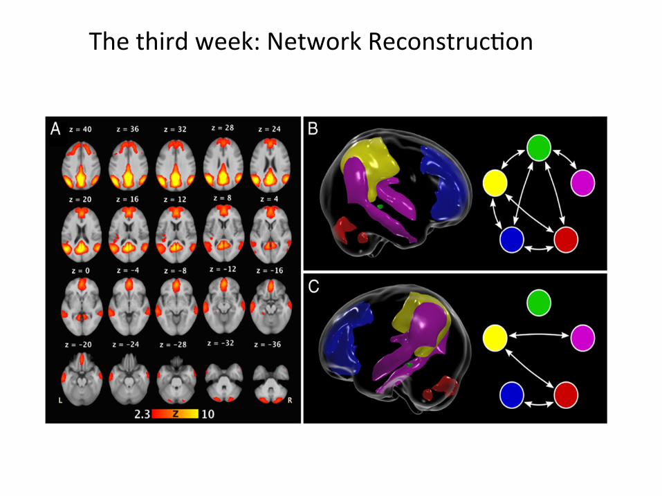
The third week: Network Reconstruc3on

Network science

A network of 800+ proteins interaction network

ver3ces and edges
• Ver3ces: genes, proteins, cells, neurons, brain regions, individuals etc.
• Edges (interac3ons): physical interac3ons, correla3ons (no direc3ons), causality (direc3on) etc.
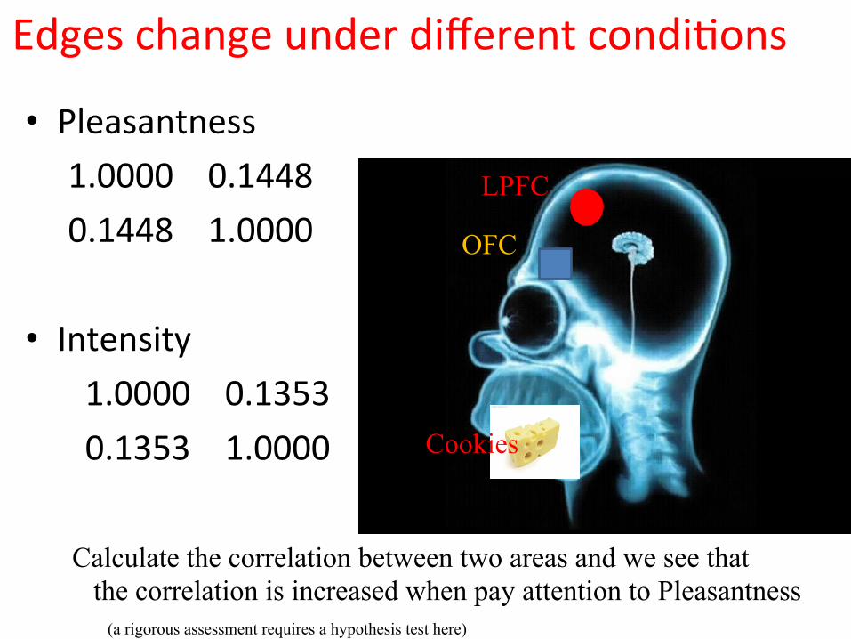
Edges change under different condi3ons
• Pleasantness 1.0000 0.1448 0.1448 1.0000
• Intensity 1.0000 0.1353 0.1353 1.0000
LPFC
OFC
Cookies
Calculate the correlation between two areas and we see that the correlation is increased when pay attention to Pleasantness (a rigorous assessment requires a hypothesis test here)
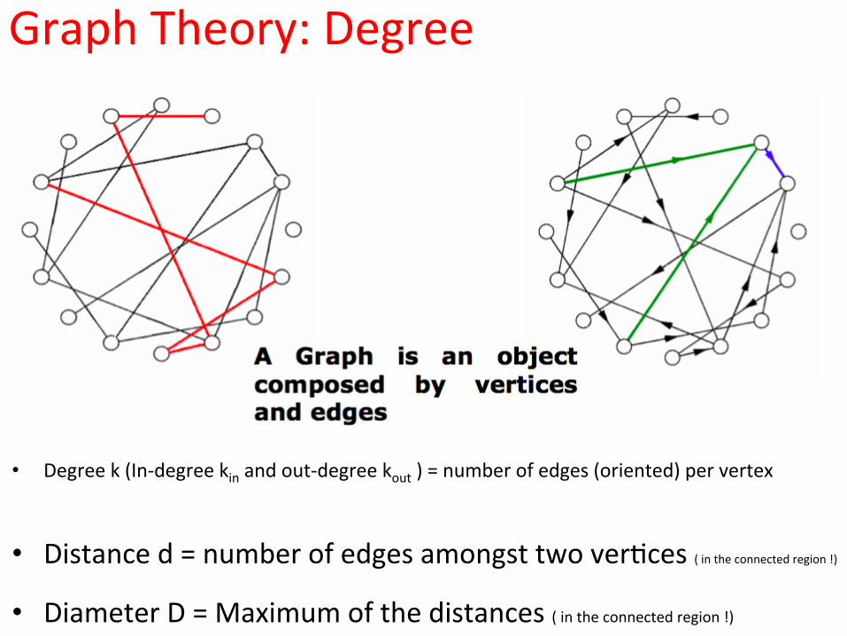
Graph Theory: Degree
• Degree k (In-‐degree kin and out-‐degree kout ) = number of edges (oriented) per vertex
• Distance d = number of edges amongst two ver3ces ( in the connected region !) �
• Diameter D = Maximum of the distances ( in the connected region !)

Graph Theory: adjacency matrices
• Adjacency Matrices: for the directed graph, the matrix is not symmetric
• Weighted graph: not only 0 and 1
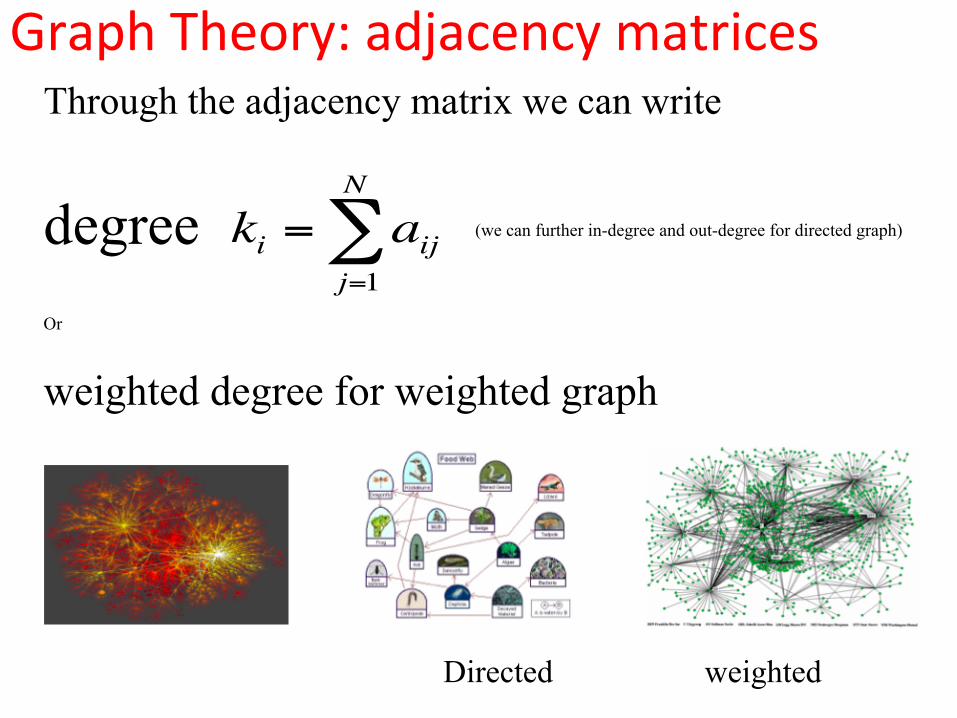
Graph Theory: adjacency matrices Through the adjacency matrix we can write
degree (we can further in-degree and out-degree for directed graph)
Or
weighted degree for weighted graph
ki = aijj=1
N
∑
Directed weighted
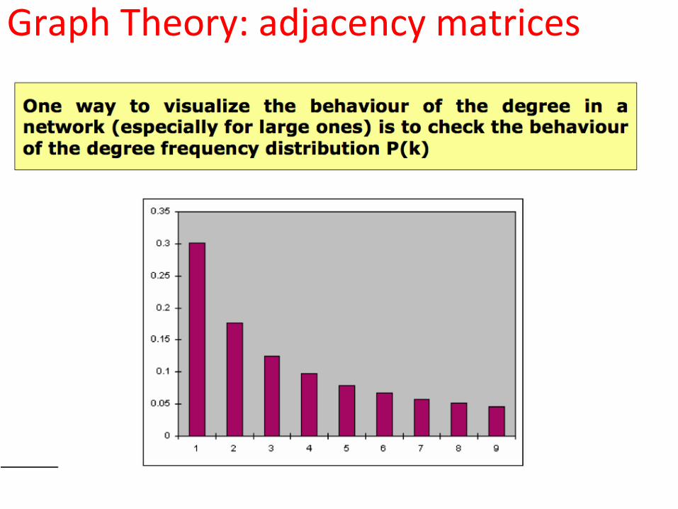
Graph Theory: adjacency matrices
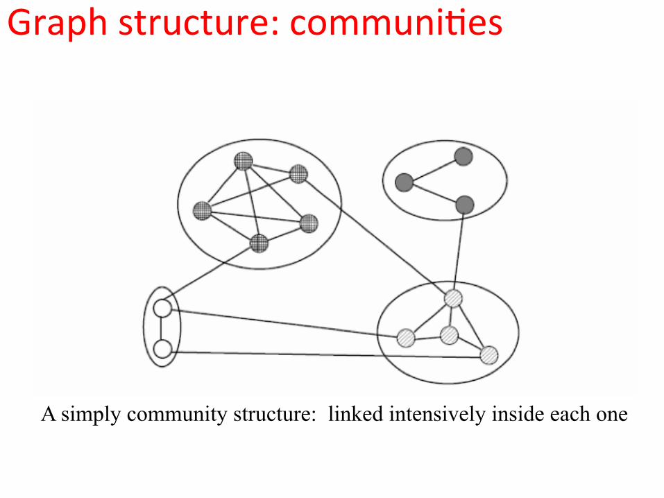
Graph structure: communi3es
A simply community structure: linked intensively inside each one
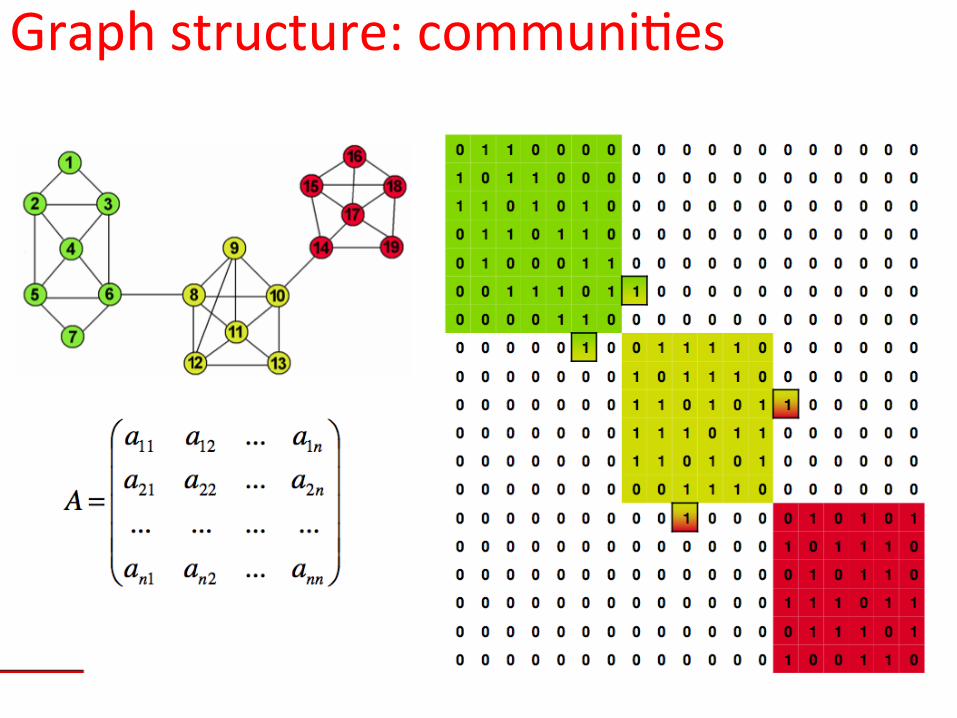
Graph structure: communi3es
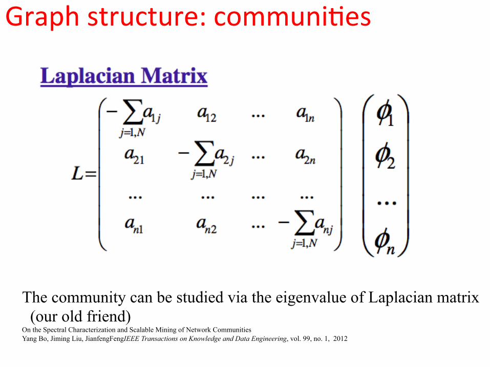
Graph structure: communi3es
The community can be studied via the eigenvalue of Laplacian matrix (our old friend) On the Spectral Characterization and Scalable Mining of Network Communities Yang Bo, Jiming Liu, JianfengFengIEEE Transactions on Knowledge and Data Engineering, vol. 99, no. 1, 2012
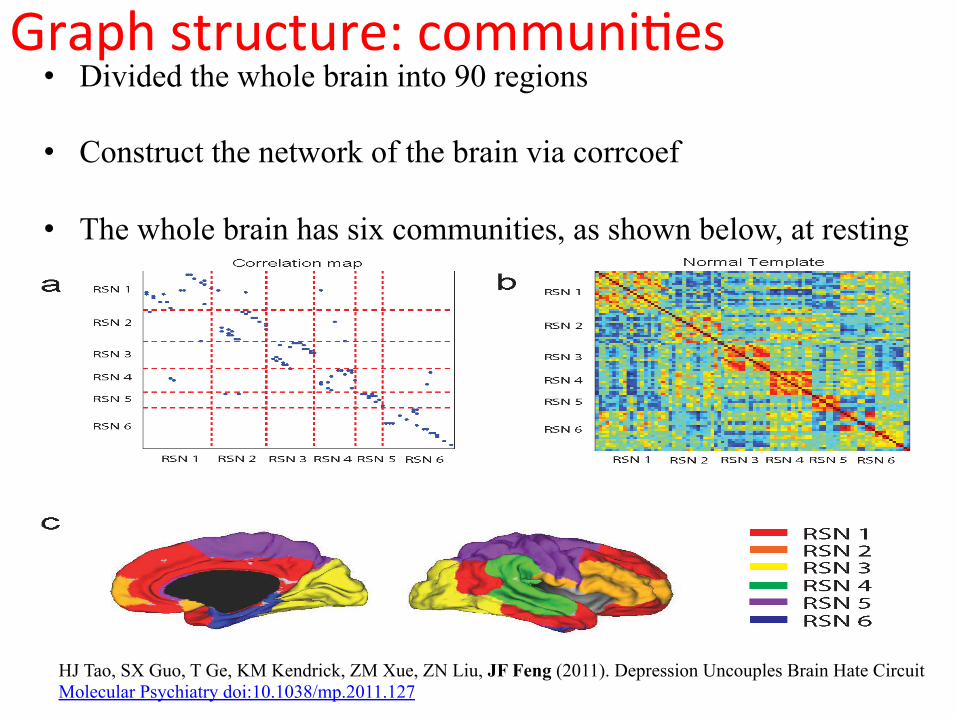
Graph structure: communi3es • Divided the whole brain into 90 regions
• Construct the network of the brain via corrcoef
• The whole brain has six communities, as shown below, at resting
HJ Tao, SX Guo, T Ge, KM Kendrick, ZM Xue, ZN Liu, JF Feng (2011). Depression Uncouples Brain Hate Circuit Molecular Psychiatry doi:10.1038/mp.2011.127

Graph structure: communi3es
Traditionally the analysis of the internet structure is via traceroutes. A few hubs are obvious and marked with bright colours.
Network Science
• This work is all so brilliant, new and exci3ng and will change the world or
• This is as old as the hills and is just a group of physicists reinterpre3ng classical results in graph theory and mixing in econometrics-‐style experiments.
• It is in-‐between
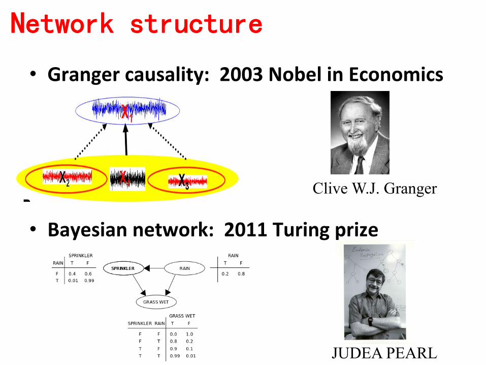
• Granger causality: 2003 Nobel in Economics
• Bayesian network: 2011 Turing prize
Network structure
Clive W.J. Granger
JUDEA PEARL

Granger causality: network structure
• Granger causality is a sta3s3cal concept of causality that is based on predic3on.
•

• Granger causality is a sta3s3cal concept of causality that is based on predic3on.
• According to Granger causality, if a signal X1 "Granger-‐causes" a signal X2, then past values of X1 should contain informa3on that helps predict X2 above and beyond the informa3on contained in past values of X2 alone.
Granger causality: network structure

• Granger causality is a sta3s3cal concept of causality that is based on predic3on.
• According to Granger causality, if a signal X1 "Granger-‐causes" a signal X2, then past values of X1 should contain informa3on that helps predict X2 above and beyond the informa3on contained in past values of X2 alone.
• Its mathema3cal formula3on is based on linear regression modeling of stochas3c processes (Granger 1969).
• Granger causality was developed in 1960s and has been widely used in economics since the 1960s.
Granger causality: network structure
• Granger causality is a sta3s3cal concept of causality that is based on predic3on.
• According to Granger causality, if a signal X1 "Granger-‐causes" a signal X2, then past values of X1 should contain informa3on that helps predict X2 above and beyond the informa3on contained in past values of X2 alone.
• Its mathema3cal formula3on is based on linear regression modeling of stochas3c processes (Granger 1969).
• Granger causality was developed in 1960s and has been widely used in economics since the 1960s.
• However it is only within the last few years that applica3ons in biology have become popular.
Granger causality: network structure

He wrote:
Prof. Clive W.J. Granger, recipient of the 2003 Nobel Prize in Economics
• The topic of how to define causality has kept philosophers busy for over two thousand years and has yet to be resolved.
Granger causality: network structure

• The topic of how to define causality has kept philosophers busy for over two thousand years and has yet to be resolved.
• It is a deep convoluted ques3on with many possible answers which do not sa3sfy everyone, and yet it remains of some importance.
Granger causality: network structure
• The topic of how to define causality has kept philosophers busy for over two thousand years and has yet to be resolved.
• It is a deep convoluted ques3on with many possible answers which do not sa3sfy everyone, and yet it remains of some importance.
• Inves3gators would like to think that they have found a "cause", which is a deep fundamental rela3onship and possibly poten3ally useful.
• In the early 1960's I was considering a pair of related stochas3c processes which were clearly inter-‐related and I wanted to know if this rela3onship could be broken down into a pair of one way rela3onships.
• It was suggested to me to look at a defini3on of causality proposed by a very famous mathema3cian, Norbert Wiener, so I adapted this defini3on (Wiener 1956) into a prac3cal form and discussed it.
• Applied economists found the defini3on understandable and useable and applica3ons of it started to appear.
Granger causality: network structure

Mathema3cal defini3on • Give you a set of data, (x(t),y(t)) • Fit the data with x(t) = a0 +a11 x(t-‐1)+…+a1p x(t-‐p) + b11 y(t-‐1) + … +b1p y(t-‐p)+ ε1t y(t) = a0 +a21 x(t-‐1)+…+a2p x(t-‐p) + b21 y(t-‐1) + … +b2p y(t-‐p)+ ε2t and x(t) = c0 +c11 x(t-‐1)+…+c1p x(t-‐p) + ξ1t y(t) = d0+ d21 y(t-‐1) + … +d2p y(t-‐p)+ ξ2t
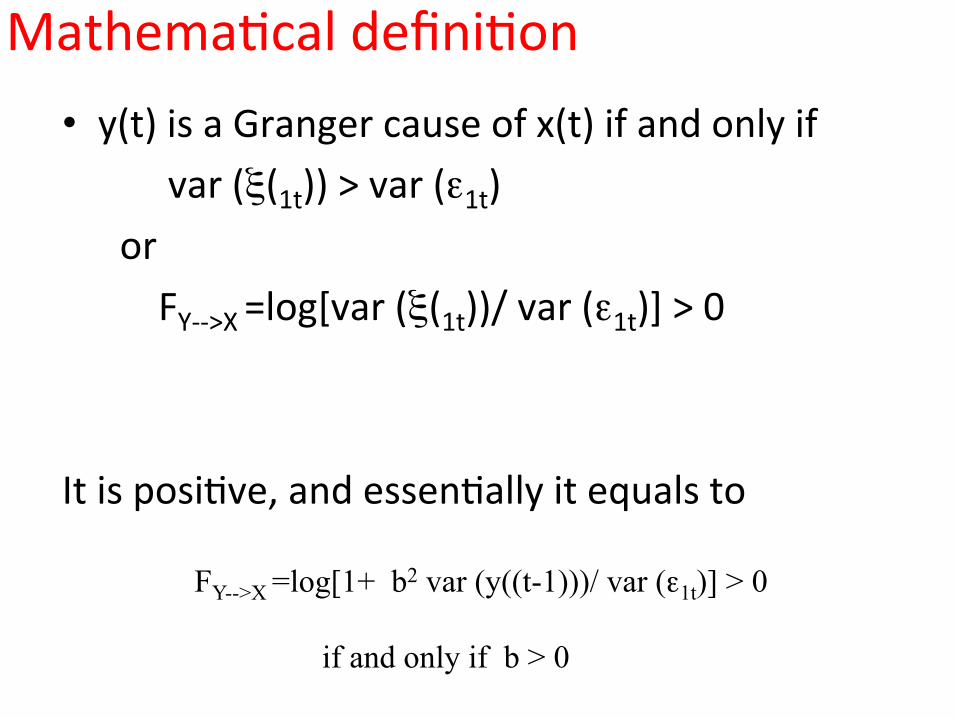
• y(t) is a Granger cause of x(t) if and only if var (ξ(1t)) > var (ε1t) or FY-‐-‐>X =log[var (ξ(1t))/ var (ε1t)] > 0 It is posi3ve, and essen3ally it equals to
FY-->X =log[1+ b2 var (y((t-1)))/ var (ε1t)] > 0 if and only if b > 0
Mathema3cal defini3on

• clear all • close all • k=2; • N=1000; • A=rand(k,2); • A=[0.1 0.5 • 0.0 0.3]; • x=zeros(N+1,k); • x(1,:)=rand(1,k); • for i=1:N • x(i+1,:)=(A*x(i,:)')'+randn(1,k); • end • plot(x(:,1)) • hold on • plot(x(:,2),'r') • abs(eig(A)) • A • AE=(x([11:N-‐9],:)'*x([10:N-‐10],:))*(in
v(x([10:N-‐10],:)'*x([10:N-‐10],:))) • co=cov(x([11:N-‐9],:)-‐
(AE*x([10:N-‐10],:)')'); • AE_Granger=[AE(1,1) 0; 0 AE(2,2)]; • cog=cov(x([11:N-‐9],:)-‐
(AE_Granger*x([10:N-‐10],:)')'); • A(1,2) • F_Y_to_X=log(cog(1,1)/co(1,1)) • A(2,1) • F_X_to_Y=log(cog(2,2)/co(2,2))
Example
x(t) = .1 x(t-1) + .5 y(t-1) + ε1 y(t) = .00 x(t-1)+.3y(t-1) + ε2 A = [ 0.1 0.5 0.0 0.3]

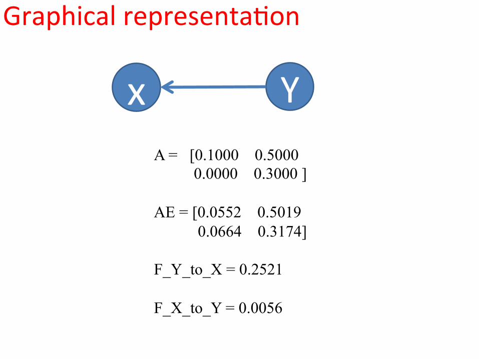
Graphical representa3on
x Y A = [0.1000 0.5000 0.0000 0.3000 ] AE = [0.0552 0.5019 0.0664 0.3174] F_Y_to_X = 0.2521 F_X_to_Y = 0.0056
How small is zero?
• Sta3s3cal test is required to see whether it is zero or not.
• Classical method can be used
• Or other non-‐parametric methods such as bootstrap can be employed

Bootsrap • Using the model (trust the model), resample it to calculate
F_X_to_Y and F_Y_to_X N 3mes
• Generate the histogram of F_X_to_Y and F_Y_to_X
• Using the confidence interval [ mean – 2 STD mean + 2 STD] to see whether 0 is in the interval above or not • If 0 is in [ mean – 2 STD mean + 2 STD] we can not reject the hypothesis that F_X_to_Y =0 otherwise, we can reject the hypothesis
Example clear all close all k=2; N=1000; A=rand(k,2); A=[0.1 0.5 0.0 0.3]; x=zeros(N+1,k); x(1,:)=rand(1,k); for i=1:N x(i+1,:)=(A*x(i,:)')'+randn(1,k); end plot(x(:,1)) hold on plot(x(:,2),'r') abs(eig(A)) A AE=(x([11:N-9],:)'*x([10:N-10],:))*(inv(x([10:N-10],:)'*x([10:N-10],:))) co=cov(x([11:N-9],:)-(AE*x([10:N-10],:)')'); AE_Granger=[AE(1,1) 0; 0 AE(2,2)]; cog=cov(x([11:N-9],:)-(AE_Granger*x([10:N-10],:)')'); A(1,2) F_Y_to_X=log(cog(1,1)/co(1,1)) A(2,1) F_X_to_Y=log(cog(2,2)/co(2,2)) A=AE; for ii=1:1000 x=zeros(N+1,k); x(1,:)=rand(1,k); for i=1:N x(i+1,:)=(A*x(i,:)')'+randn(1,k); end %plot(x(:,1)) %hold on %plot(x(:,2),'r') AE=(x([11:N-9],:)'*x([10:N-10],:))*(inv(x([10:N-10],:)'*x([10:N-10],:))) co=cov(x([11:N-9],:)-(AE*x([10:N-10],:)')'); AE_Granger=[AE(1,1) 0; 0 AE(2,2)]; cog=cov(x([11:N-9],:)-(AE_Granger*x([10:N-10],:)')'); A(1,2); F_YX(ii)=log(cog(1,1)/co(1,1)) A(2,1); F_XY(ii)=log(cog(2,2)/co(2,2)) end
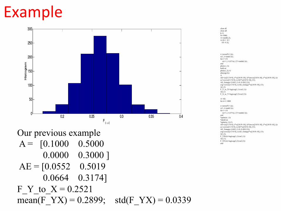
Our previous example A = [0.1000 0.5000 0.0000 0.3000 ] AE = [0.0552 0.5019 0.0664 0.3174] F_Y_to_X = 0.2521 mean(F_YX) = 0.2899; std(F_YX) = 0.0339
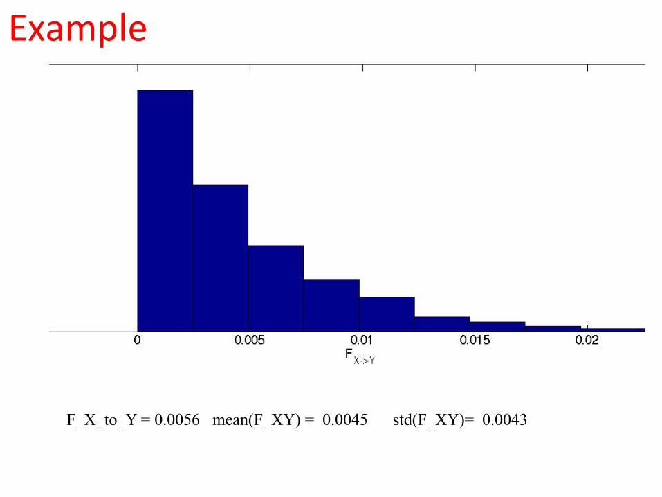
F_X_to_Y = 0.0056 mean(F_XY) = 0.0045 std(F_XY)= 0.0043
Example
Graphical representa3on
x Y A = [0.1000 0.5000 0.0000 0.3000 ] AE = [0.0552 0.5019 0.0664 0.3174] F_Y_to_X = 0.2521 F_X_to_Y = 0.0056

Other issues: par3al data
x Y
Z
x(t) = b z(t-1) + ε1
y(t) = ε2
z(t) = a y(t-1) + ε3 If z is blocked, there is no causal relationship between x and y

Other issues: par3al data • This could create a false causality if we only look at x and y or we only have x and y available
x Y
Z
x(t) = ab y(t-2) + ε4
y(t) = ε2
z(t) = a y(t-1) + ε3 If z is blocked, there is no causal relationship between x and y

Example
x Y
Z
x(t) = ab y(t-2) + ε4
y(t) = ε2
z(t) = a y(t-1) + ε3 A=[0.0 0.0 0.5 0 0 0 0.0 0.5 0];
clear all close all k=3; N=1000; A=rand(k,2); A=[0.0 0.0 0.5 0 0 0 0.0 0.5 0]; x=zeros(N+1,k); x(1,:)=rand(1,k); for i=1:N x(i+1,:)=(A*x(i,:)')'+randn(1,k); end plot(x(:,1)) hold on plot(x(:,2)+4,'r') plot(x(:,3)+8,'g') abs(eig(A)); A AE=(x([11:N-9],:)'*x([10:N-10],:))*(inv(x([10:N-10],:)'*x([10:N-10],:))) co=cov(x([11:N-9],:)-(AE*x([10:N-10],:)')'); AE_Granger=AE; for i=1:k for j=1:k if i > j AE_Granger(i,j)=0; else i<j AE_Granger(i,j)=0; end cog=cov(x([11:N-9],:)-(AE_Granger*x([10:N-10],:)')'); F(i,j)=log(cog(i,i)/co(i,i)); end F(i,i)=0; end F

Example: condi3onal Granger causality
F = causality 0 0.0006 0.3073 0.0040 0 0.0065 0.0001 0.2617 0
• Use all possible measured variables to estimate the causality rather than pairwise

Example
F = 0 0.0006 0.3073 0.0040 0 0.0065 0.0001 0.2617 0
F is certainly the adjacency matrices talked before
F = correlation = 1.1812 0.0377 -0.0057 0.0377 1.0011 0.0443 -0.0057 0.0443 1.1711
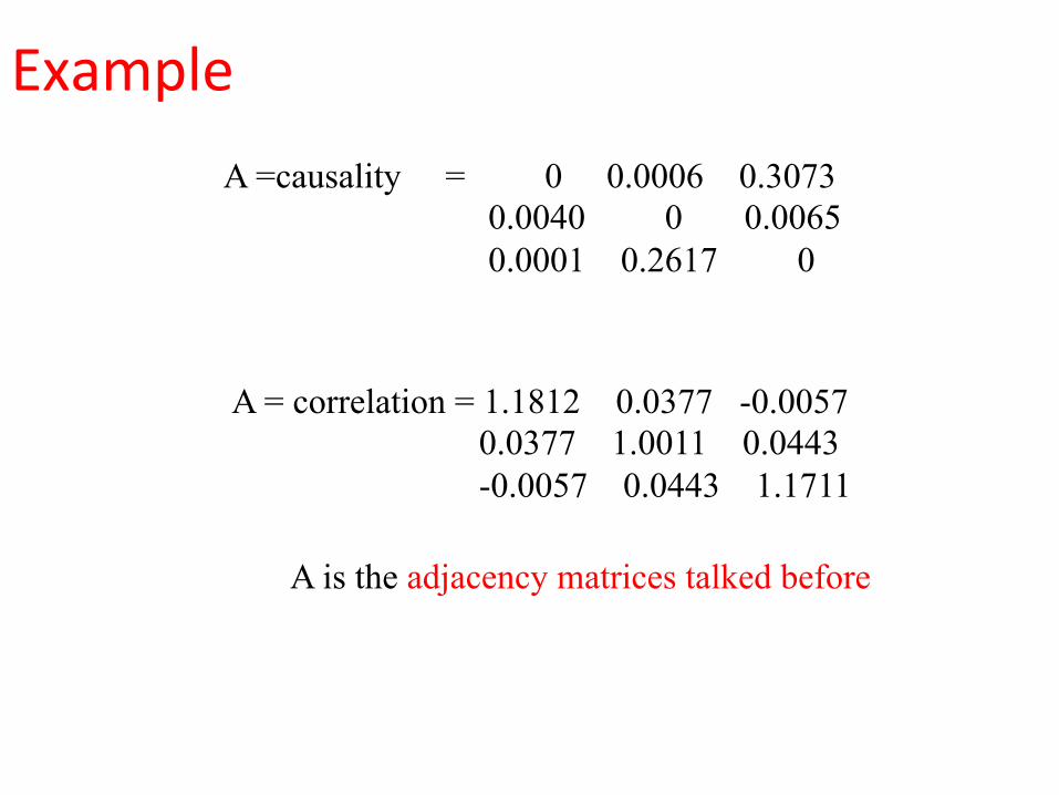
Example A =causality = 0 0.0006 0.3073 0.0040 0 0.0065 0.0001 0.2617 0
A is the adjacency matrices talked before
A = correlation = 1.1812 0.0377 -0.0057 0.0377 1.0011 0.0443 -0.0057 0.0443 1.1711
Further issues
• Common inputs: using Par3al Granger causality to get rid of common inputs
• Causality between different frequencies
• Many more, but we do not have 3me to go into details
• hsp://www.dcs.warwick.ac.uk/~feng/causality.html

seminar 3 1. For a model x(t) = b y(t-‐2) + ε1
y(t) = ε2
z(t) = a y(t-‐1) + ε3
with the matrix A=[0.0 0.0 0.4 0 0 0 0.0 0.4 0]; Generate the dataset of T=1000. a. Find the network of undirected network using correla3on. b. Find the causality matrix F. c. Interpret the results with the graphic representa3on. 2. If we only recorded (x,y) from the data, work out the causality matrix F. Interpret the results with the graphic representa3on.