Computational Analysis of a Novel Turbine Design for

Low Head Hydro Power

Undergraduate Honors Thesis

In Partial Fulfillment of the Requirement for

Graduation with Honors Research Distinction in

Mechanical Engineering at The Ohio State University

by

Thomas Malkus

April, 2019

Advisor: Dr. Clarissa Belloni

2

Abstract

A critical consideration in the design of hydro turbines is their energy conversion

efficiency. Most conventional hydro turbines operate with efficiencies up to 90%, but usually

require large heads (up to 27 meters), and large flow raters to operate efficiently. Thus,

conventional turbines are not a viable solution for low head hydropower applications such as

small dams or “weirs,” which are around 5 meters tall or less. This study presents a numerical

investigation of a novel cross-flow turbine called the William’s cross-flow turbine, which is

designed specifically for use in low head hydro power. The numerical simulations employ

Reynolds Averaged Navier Stokes Equations, using the Volume of Fluid (VOF) method to

model two phase flow through the turbine. The main set of simulations model flow over a low-

head weir and through the turbine. These simulations model the transient effects due to blade

rotation, and are used to predict the turbine efficiency. Result showed that device operated

consistently with an energy conversion efficiency of around 50%.

Design iterations were carried out with focus on blade geometry. Results showed that a

traditional “Ossberger” style cross-flow turbine blade outperformed the novel blade design that

was initially proposed. The flow field results illustrate that the turbine nozzle was not effective at

guiding the flow through the turbine, which resulted in performance reduction for both of the

blade designs that were tested.

3

Acknowledgements

I would like to sincerely thank my advisor, Dr. Belloni, for giving me the opportunity to

do this research, and for all the support and guidance along the way. Her encouragement

throughout this project has made it possible for me to work as hard as I have this year. The

amount that I have accomplished over the past year, and the skills that I have developed are

largely owed to Dr. Belloni, and I cannot thank her enough.

I owe a huge thank you to Sajjan Pokhrel for all of the help getting started on this project,

and sharing his CFD work with our research group. Sajjan’s previous work was the starting point

for the project, and without his work, I wouldn’t have gotten half as far as I did on this research.

I would also like to thank the OSU SIMCenter for supporting this research, which gave

me a huge head start on this project. Also, for their computing resources throughout the year,

which has made this work possible.

I would also like to thank our collaborators from Central State University, and KWRiver

Hydroelectic Co.: Dr. Sri, Paul Kling, and Fred Williams for the opportunity to work on this

technology. Thank you all for sharing all of your resources and expertise, which has been a huge

help on this project.

4

Contents

Chapter 1: Introduction ....................................................................................................... 6 1.1 Low Head Hydropower ...........................................................................................................6 1.2 Low Head Hydro Turbines......................................................................................................7 1.3 Thesis Objectives ................................................................................................................... 10 1.4 Literature Review ................................................................................................................. 10

Chapter 2: William’s Cross-Flow Turbine ......................................................................... 12 2.1 Overview of the Williams Cross-flow Turbine ....................................................................... 12 2.2 Previous Studies .................................................................................................................... 15

Chapter 3: Computational Method .................................................................................... 17 3.1 Governing Equations ............................................................................................................ 17 3.2 Boundary Conditions ............................................................................................................ 19 3.3 Computational Mesh ............................................................................................................. 21

3.3.1 Meshing Details......................................................................................................................... 21 3.3.2 Grid Convergence Study ........................................................................................................... 24

Chapter 4: Results .............................................................................................................. 26 4.1 Modeling Flow Over Weir ..................................................................................................... 26

4.1.1 Weir Model Validation .............................................................................................................. 26 4.1.2 Free Surface Flow at Turbine Inlet ............................................................................................ 29

4.2 Turbine Performance Characterization ................................................................................ 31 4.3 Turbine Design Study ............................................................................................................ 32

4.3.1 Base Case Design – Water Wheel Blades ................................................................................. 32 4.3.2 Second Design – Ossberger Blades ........................................................................................... 34 4.3.3 Sensitivity to Blade Inlet Angle ................................................................................................ 41

4.4 Evidence of In-effective Nozzle .............................................................................................. 43 4.5 Verification and Validation ................................................................................................... 45 4.6 Summary of Results .............................................................................................................. 45

Chapter 5: Conclusion/Future Work ................................................................................. 46

Bibliography ........................................................................................................................ 47

Appendix ............................................................................................................................. 49

5

Nomenclature

Acronyms

CFT cross-flow turbine

WCFT Williams cross-flow turbine

CFD computational fluid dynamics

RANS Reynolds-averaged Navier-Stokes equations

VOF volume of fluid

SST shear-stress transport

USBR U.S. Department of the Interior Bureau of Reclamation

NPDs non-powered dams

Lps Liters per second

RPM Revolutions per minute

Symbols

𝛼𝑖 volume fraction of ith fluid

𝛽1,2 blade inlet, outlet angle

𝜔 rotational velocity

𝜂 efficiency

𝜌 density

𝜇 dynamic viscosity

𝜃 azimuthal blade position

b width of turbine or flume

Cf weir flow correction factor

F force

H total head

Hc Height of weir crest

P power

Q volumetric flowrate

q two-dimensional flowrate

T torque

v velocity

𝑢𝑖 ith component of local velocity

Re Reynolds number

6

Chapter 1: Introduction

This chapter introduces the research by giving an overview of low head hydropower as an

alternative energy resource, as well as the current technologies used in low head hydropower

sites. The chapter closes with an outline of the research objective and a literature review of cross-

flow turbine design.

1.1 Low Head Hydropower

In 2018, hydropower made up 7% of the total electricity production, putting it at about 40%

of the energy produced from renewables (EIA.gov, 2018). Much of that power is generated from

large scale hydro-electric sites, and only about 5% of hydropower is produced from small scale

sites, which have a capacity of 10 megawatts (MW) or less. There is, however, a large potential

for the development of small scale hydropower sites. A study conducted by Oak Ridge National

Laboratory estimated the total potential capacity of non-powered dams (NPDs) in the U.S. to be

12 Gigawatts, or about 15% of the U.S.’s current total hydropower capacity (Kao,2014). The

study is based off of hydrology for sites with non-powered dams in the United States, with

potential ranging from 1-496 MW. Most relevant to the present study are dams with potential of

<10MW. Dams in the 1-10MW range have an estimated potential capacity of 2,500 MW. The

study noted that, eighty-one of the 100 top NPDs are U.S. Army Corps of Engineers (USACE)

facilities, many of which, including all of the top 10, are navigation locks on the Ohio River,

Mississippi River, Alabama River, and Arkansas River, as well as their major tributaries

(Kao,2014). It is important to note that these non-powered dams have already undergone dam

construction, so adding a turbine can be done economically and without much adverse effect on

the environment. Another technical report from Oak Ridge National Laboratory noted that most

7

of the majority of planned new small hydropower projects involve adding hydropower

generation to existing dams or conduits rather than building the dam itself (Johnson et al, 2018).

The technical report also noted that the total proposed projects (165) were small projects with a

total combined capacity of 420 MW.

Due to the relatively small amount of electric power that can be produced from small

hydro, these sites are often seen as an uneconomic source of power. A review of small

hydropower done by the Environmental Agency in Germany concluded that small hydropower

plants are uneconomic, since the cost per kwh to produce electricity is higher than the costs

payed by the Renewable Energy Act ($0.078/kWh), which is roughly the same rate payed in the

U.S. However, this study did conclude that the construction and reactivation of small

hydroelectric power plants is unproblematic at existing weirs that cannot be demolished, in

particular when ecological improvements – for instance, restoring free passage of fish – can be

achieved. (Bunge et Al., 2003).

1.2 Low Head Hydro Turbines

Many conventional turbine technologies could be installed in low head dams, however most

would be uneconomic due to the high construction costs, which also has an adverse impact on

the environment. For instance, Kaplan and Francis Turbines require large manufacture cost, and

well as construction to the leading adverse environmental impact. These turbines also have low

efficiencies at low flow rates which can be seen in Figure 1.1. Further, Kaplan and Francis

turbines usually require a head of at least 90ft (27 meters) to operate efficiently.

8

Figure 1.1: Efficiency vs. flowrate for various turbines (Sinagra et al., 2014).

Figure 1.2: Operating conditions of various turbines in terms of head and flowrate (Benzon et

al., 2016).

9

Figure 1.2 shows operating ranges for conventional hydro turbines. Note that traditional

cross-flow turbines operate at low-medium heads (2-200 meters). Cross-flow turbines are well

suited for these small applications due to their cheap and easy manufacturability compared to

other traditional turbines (Adhikari, 2016). Cross-flow turbines also have flat efficiency curves

compared to other traditional seen in figure 1.2 and thus they can perform well under a wide

range of operating conditions. However, use of traditional cross-flow turbines in low head

applications can be life threatening to the fish passing through the turbine, due to the high speed

of the blades. Also, installing a cross-flow turbine to a low head dam would likely require

modifications to the dam, and riverbed downstream.

Companies pursuing low head hydro turbines include Voith, who manufactures the

StreamDiverTM, which uses a propeller type runner and is designed for heads ranging from 2-8

meters, and outputs from 50-850 KW (Voith,2019). GE Renewables manufactures S-Kaplan and

S-Francis turbine’s with capacities as low as 5MW (GE Renewables, 2019). Others include

DIVE Turbine GmbH & Co. (2019), and Natel energy (2019). All of these turbines are low-head,

but not micro hydro, so they still produce a significant amount of energy.

There is a clear need for a turbine that can be modularly adapted to low head dams, and that

performs well under low heads. The William’s cross-flow Turbine (WCFT), being pursued by

Startup Company KW River is a potentially viable technology for these applications because it

can be installed directly beneath a low head dam, thus greatly reducing construction cost. The

simple geometry of the blades is also cheap and easy to manufacture. The design also allows it to

be modularly adapted beneath a low head dam. The energy conversion efficiency of the

William’s cross-flow turbine is crucial because it is directly related to the payback time, and thus

the practicality of using this turbine in a low head hydro power site.

10

1.3 Thesis Objectives

Since the William’s cross-flow Turbine is a novel turbine design, and no similar design

exists, the design principles for achieving high efficiencies have not yet been characterized.

The goal is to optimize the design of the WCFT, in order to determine if this novel design can

achieve efficiencies close to that of more developed turbines. Recent studies on the turbine

suggest that the turbine could be up to 80% efficient (Sritharan, 2013).

The objectives of this research are summarized as follows

Characterize efficiency of the WCFT for a rage of flow rates and turbine rotational

speeds.

Determine if the WCFT operates like a traditional cross-flow turbine. In essence is the

turbine extracting significant power at two stages in the impeller.

Optimize the blade design in effort to determine if the WCFT can achieve efficiencies

close to traditional cross-flow turbines, which operate in the 80-90% efficiency range.

1.4 Literature Review

A literature review was conducted on both experimental and numerical studies related to the

design of cross-flow turbines, in attempt to aid the design of the WCFT. The range of efficiency

found on these devices was 45% up to 90%.

Fiuzat, and Akerkar (1991) investigated the contribution of each of the two stages to the

overall power in a CFT. Results showed that the second stage contributed around 45% of the

11

overall power. Also, for a nozzle with a 90o inlet arc there was more cross-flow than the 120o

case, which resulted overall higher efficiency.

Desai (1994) conducted experimental studies on cross-flow turbines, which showed

maximum efficiencies of 84.5%. Result showed that for any runner design, the efficiency of the

turbine increase with the number of blades, however, the authors only used 25 as a maximum. It

was also shown than for an attack angle greater than 24o caused decrease in turbine efficiency.

Dakers (1982) studied the efficiencies of CFTs with 3 different nozzle geometries. Each

of the three turbines had relatively low efficiencies (45% - 69%). It was shown by Adhikari

(2016) that this was due to ineffective matching of the nozzle and runner design.

Sammartano et. Al (2013) proposed a design method for cross-flow turbines, based on initial

and final blade angles, the outer impeller diameter and the shape of the nozzle, which are

selected using a simple hydrodynamic analysis of the flow through the two stages of the

impeller. Blade design parameters were then optimized via 2D CFD simulations, employing

unsteady RANS equations in ANSYS CFX, followed by optimization of impeller to nozzle width

ratios via 3D simulations. Results showed that in this test case the turbine with 35 blades and an

attack angle equal to 22° exhibited at the design point a high efficiency η equal to 86%.

Adhikari (2016) characterized the key internal flow characteristics for both low and high

efficiency cross-flow turbines. Adhikari found that the matching of nozzle and runner designs are

the two main design requirements for high efficiency turbines. Results showed that effective

matching of these two components resulted in an efficiency improvement from 69% to 91%

(Adhikari, 2016). A ratio of r1/r2 = 0.68 (inner to outer blade radius) was also consisted among

the high efficiency designs found in literature.

12

Chapter 2: William’s Cross-Flow Turbine

This chapter gives an overview of the William’s cross-flow turbine (WCFT) and discusses

the previous studies conducted on the turbine.

2.1 Overview of the Williams Cross-flow Turbine

The WCFT can be modularly adapted beneath low head dams that have already been

built. It can also be installed along with weir, in a river that is not yet contained by weirs. Figure

2.1 shows the WCFT placement beneath a weir. This turbine is an attractive device for these

applications, since it doesn’t require alterations to the existing dam. Provided that a screen be

placed at the inlet, fish can bypass the turbine, and there is no harm to wildlife.

Figure 2.1: Diagram illustrating William’s cross-flow turbine at the beneath a low head weir

The Williams cross-flow turbine is close in functionality to the breastshot water wheel as

well as the traditional Ossberger cross-flow turbine. Breastshot water wheels can have

efficiencies of 80-85% (Muller, 2004). Note however that the diameter of the WCFT is much

Blades Extract Power

Natural Flow Over Weir

13

smaller that of a breast shot water wheel (see figure 2.2). Breastshot water wheels typically have

an outer blade diameter that is equal to about twice the upstream head (Muller, 2004). Figure 2.1

above shows the WCFT impeller is at most half of the upstream water height.

Figure 2.2 Breastshot water wheel (Muller, 2004).

Thus, the impeller rotational speed is typically much faster of the WCFT is much faster than a

water wheel. Also, most of the energy is converted to kinetic energy before hitting the WCFT

blades, where as a water wheel blade is at a height such that most of the energy is still potential

energy that is carried down by the wheel.

The traditional cross-flow turbine, shown in figure 2.3, has been well studied, and

designs have been well revised to achieve efficiencies of up to around 90%. The effectiveness of

these devices is largely due to the double passage of flow through the blades. The William’s

cross-flow turbine is similar to a traditional cross-flow turbine in that it extracts power at 2 stages

14

in the impeller, which is shown in chapter 4. However, the portion of the rotor which extracts

power is much smaller than a traditional cross-flow turbine. This is due to the nozzle of the

cross-flow turbine, which guides the flow such that the water entering the turbine meets the

blades at a constant attack angle, as shown in figure 2.3.

Figure 2.3: Traditional cross-flow turbine (Cink-hydro-energy, 2019).

Also, the outlet of the WCFT is submerged in the downstream water, whereas the outlet

of an Ossberger type cross-flow turbine is open to the atmosphere. This allows the passage of

water through the second stage of turbine blades due to the gravity pulling the water downward

through the second passage.

15

2.2 Previous Studies

To date, previous studies have only been conducted on the lab scale model WCFT shown

in figure 2.4. Experimental studies by Sritharan (2013) were done using the belt tensioner set up

shown below to measure torque, and power. This study showed the turbine could be up to 80%

efficient, however the study used an efficiency definition different than the present study. (See

section 4.2 for efficiency definition).

Figure 2.4: Lab Scale Model of Williams Cross-Flow Turbine in Experimental Flume

Sajjan Pokhrel (2017) conducted a numerical study on the lab scale Williams cross-flow

turbine shown in figure 2.4. The study employed 3D, unsteady RANS simulations using the

Volume of Fluid (VOF) model in ANSYS Fluent. His results showed that a 9-bladed impeller

outperformed a 12-bladed impeller. These results were specific to only one operating condition,

however they illustrate the ability to predict free surface flow through such a turbine using CFD.

The present study investigates the WCFT at multiple operating conditions (flow rates), and

investigates new blade designs and compares the power output to original design developed by

16

KWRiver Hydroelectric Co. Geometry of the laboratory scale turbine and weir setup is shown in

figure 2.5. This is the prototype that all previous numerical and experimental work has been

conducted on thus far. All simulations as a part of this work use the lab scale weir and casing

geometry in figure 2.5.

Figure 2.5: Laboratory scale turbine weir setup. Dimensions are in mm. The width of the

turbine into the page is 0.15m. Drawing taken from Sritharan (2013).

17

Chapter 3: Computational Method

This chapter discusses the computational method used to model the William’s cross-flow

turbine. The approach employed in this study uses a moving mesh in a rotating reference frame

in ANSYS Fluent. The CFD method used in this study was adapted from the work done by

Sajjan Pokhrel (2017). Pokhrel’s simulations model the WCFT staring from the inlet of the

turbine and ending at the turbine outlet. In order to accurately model multiple flow rates, this

work models the weir in conjunction with the turbine. A separate set of simulations was

performed on the weir alone in order to verify to the method. The main set of simulations include

the weir and the turbine, which were used to calculated the resulting torque on the turbine blades

over a range of angular velocities to predict the peak power and efficiency of the turbine.

3.1 Governing Equations

This study employs the Reynolds Averaged Navier Stokes equations, in unsteady form, or the

URANS equations:

Continuity: 𝜕𝑢𝑖

𝜕𝑡+

𝜕𝑢𝑖

𝜕𝑥𝑖 = 0 (3.1)

Momentum: 𝜌𝜕𝑢𝑖

𝜕𝑡+ 𝜌𝑢𝑗

𝜕𝑢𝑖

𝜕𝑥𝑗= −

𝜕𝑝

𝜕𝑥𝑖+

𝜕

𝜕𝑥𝑗 [𝜇 (

𝜕𝑢𝑖

𝜕𝑥𝑖+

𝜕𝑢𝑖

𝜕𝑥𝑗) − 𝜌𝑢′𝑖𝑢𝑗

′̅̅ ̅̅ ̅̅ ̅̅ ] (3.2)

Here �̅�𝑖 is the ith component average velocity, i = 1,2,3 , p is pressure, 𝜌𝑢′𝑖𝑢𝑗′̅̅ ̅̅ ̅̅ ̅̅ is the Reynolds

shear stress, which results from breaking velocity into its average and fluctuating components. In

the present study, the Reynolds stresses are modeled using k𝜔 –SST model, which is a popular

model involving flow separation. This model has been used and validated in simulations

18

involving multiphase flow through cross-flow turbines (Adhikari, 2016). The 𝑘 − 𝜖 model has

also been used in modeling cross-flow turbines, but this model has been known to produce

inaccurate results for flow involving large amounts of separation (ANSYS, 2016).

To model the free surface flow through the turbine, the Volume of Fluid (VOF)

multiphase model was employed, which uses a continuity equation to track the interface of two

or more fluids. For the two fluids, water and air, used in this study, the volume fraction equations

are

1

𝜌𝑤[𝜕

𝜕𝑡(𝛼𝑤 𝜌𝑤) +

𝜕

𝜕𝑥𝑖(α𝑤𝜌𝑤𝑣𝑖,𝑤) ] = 0 (3.3)

𝛼𝑎 = 1 − 𝛼𝑤 (3.4)

where 𝛼𝑤 and 𝛼𝑎 are the volume fraction of water and air respectively. ANSYS Fluent solves the

continuity equation (eq. 3.3) for the secondary phase which was set to water. However for air

(the primary phase) the volume fraction is calculated by the constraint in equation 3.4 (ANSYS,

2016). As a test case, water was set as the primary phase in Fluent, and this had no effect on the

final solution. The momentum equation that is solve (equation 3.2) then uses weighted properties

of 𝜇 and 𝜌, which are weighted by the volume fraction in that cell. Thus, for the cells which have

a water volume fraction of 1, the equations in those cells are simply the RANS equations for

water. Implicit discretization of the VOF equations was used, which uses the volume

fraction, 𝛼𝑤, at the current time step when calculating the spatial part of equation 3.3 (second

term on left hand side of equation). This is opposed to the explicit scheme which uses 𝛼 at the

previous time step. Explicit – time marching – methods are typically recommended for time

dependent calculations (ANSYS, 2016), however, the implicit scheme is more robust for larger

time steps. The time step used in explicit calculations is determined by the Courant number,

19

𝛥𝑡/(𝛥𝑥/𝑣𝑓𝑙𝑢𝑖𝑑), near the interface of the fluids. The default ANSYS Fluent uses is 0.25, and it

should be at least less than 1 (ANSYS, 2016). For the small cells in the near blade regions, this

would result in extremely small time steps (~10-6 seconds). Thus, implicit method was employed,

which was also used by Pohkrel (2017).

3.2 Boundary Conditions

Modeling the turbine starting from the inlet requires velocity, or pressure be known at the

inlet of the turbine. Both approaches have been used to model cross-flow turbines, and results

have shown good agreement with experiment for each case (Sammartano el al., 2013, Adhikari,

2016). However, for the free surface flow over the weir, the velocity at the turbine inlet is not

exactly known. The velocity at the inlet can be estimated as 𝑣 = √2𝑔Δℎ, which was the method

used by Pokhrel (2017). However, since the rate of kinetic energy delivered for a given flow rate

is P =1

2𝜌𝑄𝑣2, the resulting uncertainty in the power is

𝛿𝑝

𝑃 = 2

𝛿𝑣

𝑣 . So, for an estimated velocity

of +/- 5%, which is a reasonable uncertainty, the resulting uncertainty in power for a typical

operating condition is +/- 10%, in addition to the other uncertainties in the model. Since the

upstream head water flowing over a weir is directly related to the flowrate through the turbine,

and since the upstream flowrate is what is controlled in the lab, it is important to model both

accurately. Therefore, the simulations in this work model the flow over the weir, and through the

turbine inlet.

20

Figure 3.1 Boundary conditions

Inlet

The velocity at the inlet was set such that the 2-dimensional flow rate was equal to the

values measured in the laboratory using an orifice flow meter at steady state conditions, taken

from (Sritharan, 2013). The volume fraction of water at this location is set as 1. The inlet

boundary was partitioned so that the velocity inlet portion is at a height lower than the weir. The

top portion of this boundary was set to a no slip wall condition, such that the height of the water

level can rise, which is dependent on the flowrate at the inlet. Once the height of the water

stopped changing, the flow into the turbine also reaches a steady state. This method is validated

in section 4.1.1.

For traditional cross-flow turbines, inlet conditions used are typically velocity inlets, or

total pressure conditions at the inlet of the nozzle (Sammartano et. Al, 2013, Adhikari, 2016).

However, in a traditional cross-flow turbine, the flow is fully developed at the inlet of the turbine

nozzel, and there is no complication due to the free surface as in the WCFT.

21

Outlet

The outlet boundary was set as a 0 gauge pressure (1 atmosphere), but far enough

downstream (approximately 1H) so that the flow immediately after the turbine is not effected.

The entire top boundary is also set at 0 gauge pressure.

Walls

The walls in this domain are the blades, turbine casing, weir, flume floor, and top portion

of the inlet. Each wall is set as a no slip, adiabatic wall. For the case of the turbine blades, the no

slip condition implies that the normal and tangential velocity components are zero in the rotating

fame.

Interface

The boundaries of the rotating fluid zone, and stationary fluid zone are set as an interface

in Ansys fluent. At this boundary cell faces from the rotating zone at this boundary “slide” with

respect to those of the stationary zone. Thus, nodes of the two regions do not line up at this

region, and a non-conformal boundary condition is applied at the two faces (ANSYS, 2016).

3.3 Computational Mesh

3.3.1 Meshing Details

2-Dimensional Geometries of the blades, casing, and weir were created in SolidWorks

(geometry details are shown in figure 2.2), and the geometry was meshed using ANSYS design

modeler. An unstructured, quadrilateral-dominant (mostly quadrilateral, with some triangles)

mesh was generated in the domain, with increased refinement close to the turbine/weir as seen in

22

figure 3.2. Note that in the stationary portion of the turbine shown in figure 3.3 a, there is a very

small annular portion between the wall and the interface. The annular portion should be meshed

as a part of the stationary zone, so that the surface of the rotating zone is in contact with the

stationary zone at all points around the circle. The need to mesh that portion as part of the

stationary zone requires considerable effort. Overall, the minimum orthogonal quality of the

mesh was 0.20, and the maximum skewness was 0.76.

Figure 3.2: Computational mesh

Figure 3.3 a: Turbine casing zone (stationary) b: Rotating fluid zone

The rotating zone shown in figure 3.3 b consists of the turbine blades which rotate at a

prescribed angular velocity, using the sliding mesh technique in ANSYS Fluent. For turbo

23

machinery applications, the grid should be resolved near the blades in order to capture important

turbulence features in these regions (Adhikari, 2016). The k-omega SST model in ANSYS fluent

uses enhanced wall treatment, meaning that for finely spaced near wall grid points, the

appropriate low-Reynolds number boundary condition is applied, while for course near wall grid

points a wall function approach is used (ANSYS,2016). In order to properly resolve the viscous

sublayer using the k-omega SST model, y+ in equation 2.1 should be close to 1.

𝑦+ =𝑦𝑝𝜇𝑡

𝜈 (2.1)

Here, 𝑦𝑝 is the distance to each wall adjacent cell center, and 𝜇𝑡 can be estimated by the

expression:

𝜇𝑡 ≈ 𝑈∞ √Cf

2 (2.2)

Where U∞ is the free stream velocity near the blade region and the skin friction coefficient Cf

can be estimate empirically as:

𝐶𝑓

2 ≅

0.032

𝑅𝑒14

(2.3)

For cross-flow turbines, Re has been based off of the chord length of the blade (Adhikari, 2016).

Performing this calculation by setting y+ = 1 gives a first height yp = 0.01mm. The confirmed

value of y+ after the simulation was run showed that y+ was mostly around 0.3-0.9, and had a

maximum value of 1.2 occurring only at the tips of the blades.

24

3.3.2 Grid Convergence Study

Simulations were carried out with the 4 mesh sizes in table 3.1, and the blade torque was

monitored for each case. The solution was considered grid independent when the difference

between average torques computed from two consecutive mesh sizes was <1%, which is a

reasonable level of engineering accuracy. Note also that for the design portion of this study,

improvements in power less than 1% will be considered insignificant. Each simulation was

carried out for 6 seconds, at which the torque monitor oscillated periodically about a mean value

as shown in figure 3.4. The percent change in power between the 170k and 230k-cell simulations

was 0.2% as shown in Table 3.1. Therefore, the 170K-cell mesh was used for the remainder of

the work. This mesh used a cell size of 1.5mm in the rotating impeller region and turbine casing,

and 4mm away from the weir turbine region. The total number of cells slightly differed for the

different blade designs, but cell sizes were the same.

Table 3.1: Average blade torque vs. mesh size

Number of Cells Average Torque

(N-m) % Change (Ti+1-Ti)/Ti

67,000 0.846 6.2%

110,000 0.896 -2.59%

170,000 0.875 0.205%

230,000 0.878

Figure 3.4 shows a plot of the total torque vs. time for the 170K-cell simulation. The

average value is calculated from the last 2 seconds from the simulation, where it appears to be

oscillating at about a steady value. Figure 3.5 shows the torque on a single blade vs. time, for the

last 4 full revolutions. Note that there are some non-uniformities, due to water sloshing, however

the torque on a single blade appears periodic as expected. The time step used in the simulations

was 0.0005 seconds.

25

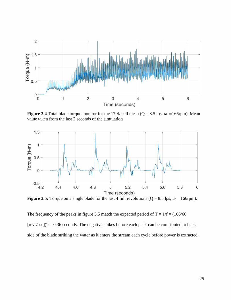
Figure 3.4 Total blade torque monitor for the 170k-cell mesh (Q = 8.5 lps, 𝜔 =166rpm). Mean

value taken from the last 2 seconds of the simulation

Figure 3.5: Torque on a single blade for the last 4 full revolutions (Q = 8.5 lps, 𝜔 =166rpm).

The frequency of the peaks in figure 3.5 match the expected period of T = 1/f = (166/60

[revs/sec])-1 = 0.36 seconds. The negative spikes before each peak can be contributed to back

side of the blade striking the water as it enters the stream each cycle before power is extracted.

26

Chapter 4: Results

This chapter presents the simulation results of the initial blade design, as well as a blade

design based off of a traditional ossberger cross-flow turbine. This chapter also shows that the

WCFT does extract power at 2 stages in the impeller, which was unknown at the start of this

research. Lastly, it is shown that the inlet of the turbine is ineffective; a new nozzle design is

proposed at the end of the chapter.

4.1 Modeling Flow Over Weir

This section validates the model of free surface flow over the weir in 2 Dimensions,

which is a crucial step in predicting the power output, such that it accurately represents the

laboratory scale turbine for a given flow rate. The measured velocity field at the inlet of the

turbine was then compared to the ideal case in which all of the gravitational potential is

converted to kinetic energy.

4.1.1 Weir Model Validation

An analytical expression for the volumetric flow rate over a weir can be derived from

Bernoulli’s equation, assuming atmospheric pressure above the weir crest. The flow over a (Q) is

related to the water level above the crest (H) by:

𝑄 =2

3√2𝑔𝑏𝐻

3

2 (4.1)

Where b is the width of the channel or flume (Munson, 2012).

27

In real applications, the flow over a weir differs from Q by a correction factor 𝐶𝑓, so that:

𝑄𝑎𝑐𝑡𝑢𝑎𝑙 = 𝐶𝑑2

3√2𝑔𝑏𝐻

3

2 (4.2)

= 𝐶𝑓𝑏𝐻32

The closest traditional weir geometry to the geometry in the experimental flume is known as an

Ogee-weir, which has a value of 𝐶𝑓= 2.18 (USBR, 1987).

Simulations were ran for various upstream velocities as an input, along with a constant

water volume fraction of one at the inlet. Thus, changing the velocity (and thus the flowrate) at

the inlet will result in a different water height, which should satisfy equation 4.2. Figure 4.1

shows the volume fraction contours once the solution has reached a steady state. The

superimposed streamlines show the path of water from inlet over the weir.

Figure 4.1: Stream lines superimposed on water volume fraction contours for flow rate of 0.0459

m2/s, or 13.77 x10-3 m3/s for the flume width of b =0.3m.

When the solution reached a steady state, the mass flow at the outlet was equal to that at

the inlet. The height of the water upstream of the weir was measured then measured. Results are

28

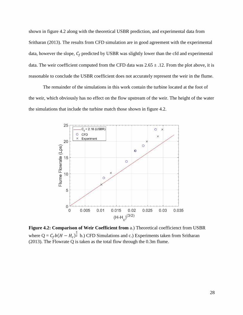
shown in figure 4.2 along with the theoretical USBR prediction, and experimental data from

Sritharan (2013). The results from CFD simulation are in good agreement with the experimental

data, however the slope, 𝐶𝑓 predicted by USBR was slightly lower than the cfd and experimental

data. The weir coefficient computed from the CFD data was 2.65 ± .12. From the plot above, it is

reasonable to conclude the USBR coefficient does not accurately represent the weir in the flume.

The remainder of the simulations in this work contain the turbine located at the foot of

the weir, which obviously has no effect on the flow upstream of the weir. The height of the water

the simulations that include the turbine match those shown in figure 4.2.

Figure 4.2: Comparison of Weir Coefficient from a.) Theoretical coefficienct from USBR

where Q = 𝐶𝑓𝑏(𝐻 − 𝐻𝑐)3

2 b.) CFD Simulations and c.) Experiments taken from Sritharan

(2013). The Flowrate Q is taken as the total flow through the 0.3m flume.

29

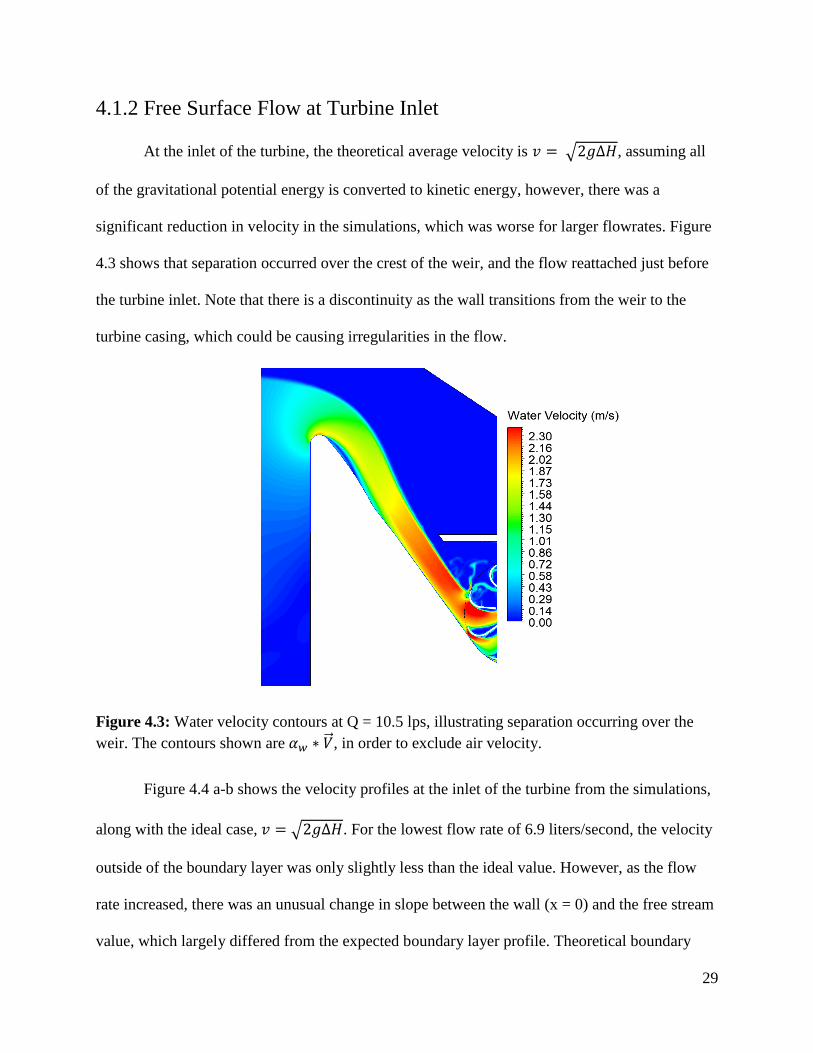
4.1.2 Free Surface Flow at Turbine Inlet

At the inlet of the turbine, the theoretical average velocity is 𝑣 = √2𝑔Δ𝐻, assuming all

of the gravitational potential energy is converted to kinetic energy, however, there was a

significant reduction in velocity in the simulations, which was worse for larger flowrates. Figure

4.3 shows that separation occurred over the crest of the weir, and the flow reattached just before

the turbine inlet. Note that there is a discontinuity as the wall transitions from the weir to the

turbine casing, which could be causing irregularities in the flow.

Figure 4.3: Water velocity contours at Q = 10.5 lps, illustrating separation occurring over the

weir. The contours shown are 𝛼𝑤 ∗ �⃗� , in order to exclude air velocity.

Figure 4.4 a-b shows the velocity profiles at the inlet of the turbine from the simulations,

along with the ideal case, 𝑣 = √2𝑔Δ𝐻. For the lowest flow rate of 6.9 liters/second, the velocity

outside of the boundary layer was only slightly less than the ideal value. However, as the flow

rate increased, there was an unusual change in slope between the wall (x = 0) and the free stream

value, which largely differed from the expected boundary layer profile. Theoretical boundary

30

layer profiles are shown in appendix A1. This unusual change in slope can be seen in the velocity

contour in figure 4.3, which shows that the flow slightly separated over the weir, and then re-

attached before it entered the turbine. The slope on the right side of the plot is due to the gradient

of the volume fraction of water 𝛼𝑤.The reduction factor of average velocity at the inlet, �̅�/𝑣𝑖𝑑𝑒𝑎𝑙,

respectively for the three cases was 0.950, 0.945, and 0.93

(a) Q = 6.9 Lps (b) Q = 8.5 Lps (c) Q = 10.5 Lps

Figure 4.4: Velocity profile at turbine inlet vs. theoretical ideal velocity, √2𝑔Δ𝐻. X is the

horizontal distance from the wall, since points on this line have the same theoretical velocity.

The losses in kinetic energy occurring before the turbine inlet are not counted when calculating

the turbine efficiency, which is defined in the next section.

31

4.2 Turbine Performance Characterization

The hydrodynamic efficiency of the turbine is defined as

𝜂 = 𝑆ℎ𝑎𝑓𝑡 𝑃𝑜𝑤𝑒𝑟

𝐴𝑣𝑎𝑖𝑙𝑎𝑏𝑙𝑒 𝑃𝑜𝑤𝑒𝑟 =

𝑇𝜔

𝜌𝑔Δ𝐻𝑄 (4.4)

The theoretical head difference, Δ𝐻 is the difference between H1 and H2 as shown in figure 4.5.

However, as noted in section 4.1.2, significant reduction in head difference was seen before the

inlet of the turbine. Therefore, the effective upstream head was taken as

𝐻1′ = 𝐻𝑖𝑛 +

<𝑣2>

2𝑔 (4.5)

where ⟨𝑣2⟩ is the average square of the velocity at the inlet of the turbine. Since the simulations

are two dimensional, the torque and flowrate are computed using the turbine width, 0.15 meters.

Figure 4.5: Water volume fraction contours illustrating upstream and downstream heights used

for efficiency calculation.

𝐻1

𝐻2

𝐻𝑖𝑛

𝐻1′

32

4.3 Turbine Design Study

In this section, the base case water-wheel like blade design is evaluated, and then

compared to an Ossberger style blade at various inlet angles. Blade design iterations were

stopped once it was realized that the nozzle was ineffective at guiding the flow through the

blades, which is causing a reduction in efficiency. Attempt to redesign the nozzle was made,

which is part of ongoing work.

4.3.1 Base Case Design – Water Wheel Blades

The base case design which was original investigated by Sritharan (2013) and Pokhrel

(2017), is shown in figure 4.6. With this blade design, the WCFT closely resembles a breast shot

water wheel, but with the blades detached from the shaft.

Figure 4.6: Geometry of the initial impeller and casing design provided by KW River

Hydroelectric Co.

Design

Parameter

Value

Blade number 9

𝑅1 34.3 mm

𝑅2 76.2 mm

𝑅3 15.4 mm

𝑅3

𝑅2 𝑅1

33

For the base case design, the simulations were run at the operating conditions taken from

Sritharan (2013), which are shown in table 4.1. In the experiments, however, there was a large

uncertainty in the flowrate measurements, which made it too difficult to compare the

experimental results with simulation results.

Table 4.1: Simulated operating conditions

Figure 4.7 shows the power curves for each flow rate tested. Note that for each flowrate,

the peak power occurs at roughly the same rotational speed of 180 rpm. However, for the 10.5

lps simulation, the curve was slightly steeper, i.e. there is a smaller range for peak power. The

fact that the peaks do not shift much is due to that fact that the upstream head H, does not change

much, for each flowrate, and therefore, the velocity of the incoming water is roughly the same. A

significant increase in water velocity relative to the blade would likely shift the peak over. In the

13 lps simulation, the casing was flooded with water and the power output of the turbine

decreased essentially to zero.

The efficiency was around 50% for each case. Note that the efficiency slightly decreased

as flowrate increased, which was the case for every blade design tested, and is discussed further

detail in the next section.

Operating Condition Value

Upstream Head (𝐻) , [mm]

Flow Rate Q, [lps]

425

6.9

Upstream Head (𝐻) , [mm]

Flowrate Q, [lps]

433

8.5

Upstream Head (𝐻) , [mm]

Flowrate Q, [lps]

446

10.5

Upstream Head (𝐻) , [mm]

Flowrate Q, [lps]

458

13

Rotational Speed 𝜔, [RPM] 120 – 240

34

Figure 4.7: Power output vs. rotational speed for the original turbine design, for flow rates 6.9,

8.5, and 10.5 liter per second. Flow rates are stated using the width of the laboratory scale

turbine b = 0.15 meters.

4.3.2 Second Design – Ossberger Blades

The first new blade design tested was based of the blades used in an Ossberger or Banki-

Michell turbine. The 2-dimensional geometry is shown in figure 4.8 below. The value of 𝛽1= 49o

was chosen such that as the blade makes first contact, the stream is parallel to the leading edge of

the blade. The rest of the parameters used in the design were taken from literature on cross-flow

turbines as discussed in section 1.4.

𝜼𝒎𝒂𝒙 = 𝟓𝟏%

𝜼𝒎𝒂𝒙 = 𝟓𝟐%

𝜼𝒎𝒂𝒙 = 𝟓𝟒%

35

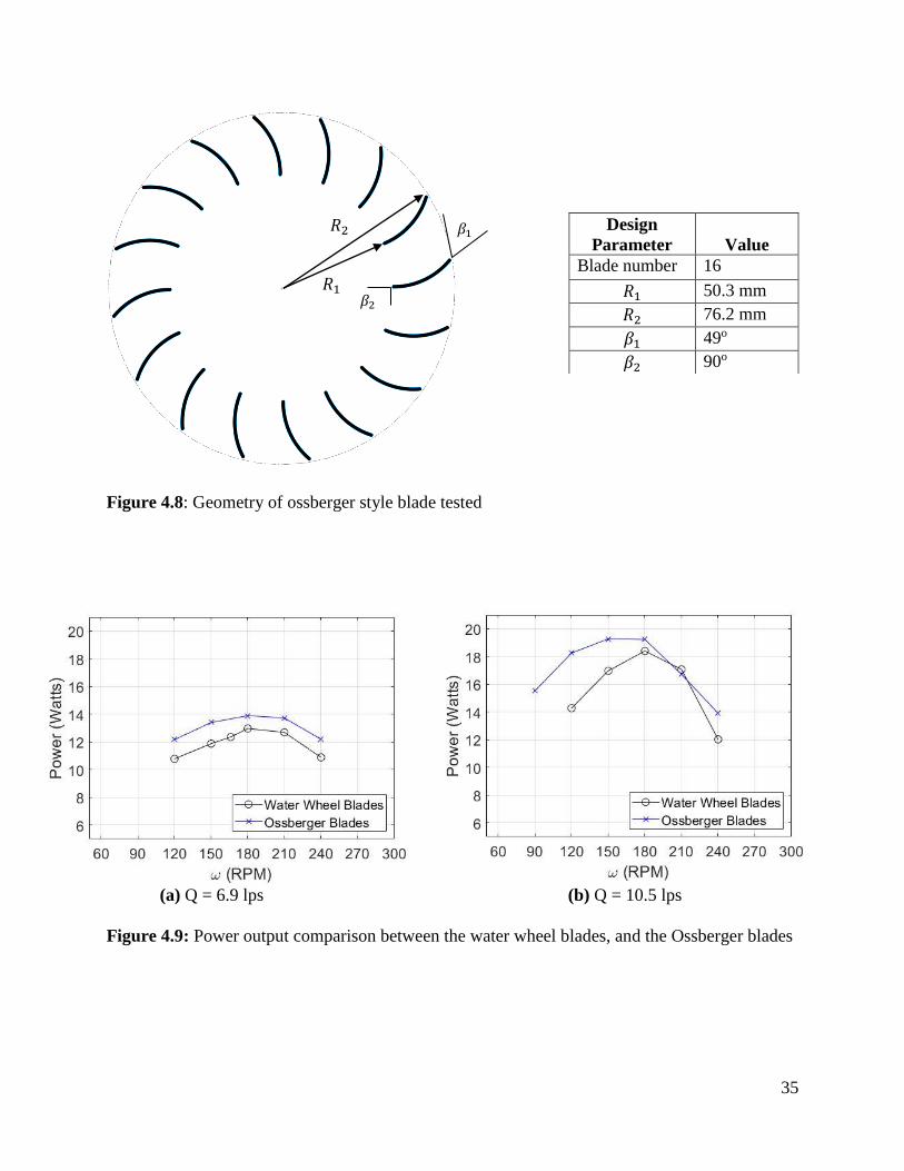
Figure 4.8: Geometry of ossberger style blade tested

(a) Q = 6.9 lps (b) Q = 10.5 lps

Figure 4.9: Power output comparison between the water wheel blades, and the Ossberger blades

Design

Parameter

Value

Blade number 16

𝑅1 50.3 mm

𝑅2 76.2 mm

𝛽1 49o

𝛽2 90o

𝛽1

𝛽2

𝑅2

𝑅1

36

Figure 4.9a shows that at a low to mid-range flow rate of 6.9 Liters/sec the Ossberger

type blades outperformed the Water Wheel type blades. For this case, the power output was

increased 7.1% with the Ossberger blade. At the maximum flowrate of 10.5 lps, the power output

was increased 4.7%, however, the peak occurred at a slightly lower angular velocity. Note also

that the curve corresponding to the Ossberger blade in figure 4.9b is slightly wider, indicating a

larger range of optimal rotational speeds.

The set of plots showing the torque vs. time plots in figure 4.10 illustrate why the

Ossberger blade outperformed the water wheel blade for the low range flow rate. Each plot

shown in figure 4.10 and 4.11 correspond to the optimum rotational speed of 180 RPM. For the

low flow rate case of 6.9 liters/sec, the water wheel blade showed significantly larger

oscillations, due to impulses to the rear side of the blade causing an opposing torque. Also, the

Ossberger design uses more blades (16 vs. 9), so the impulses from the water jet are more

frequent, causing less variation in the total torque in figure 4.10 (b). Observe, however that for

the maximum flow rate case of 10.5 liters/sec shown in figure 4.11 that the two blade designs

showed roughly oscillation amplitude and mean torque value.

37

(a) Water Wheel Type Blades (b) Ossberger Type Blades

Figure 4.10: Total blade torque from last 2 seconds of simulation, for the minimum flowrate Q =

6.9 lps and optimal speed of 180 RPM

(a) Water Wheel Type Blades (b) Ossberger Type Blades

Figure 4.11: Total blade torque from last 2 seconds of simulation, for the minimum flowrate Q

= 10.5 lps and optimal speed of 180 RPM

Q = 6.9 LPS

Q = 10.5 LPS

38

In the contour plots of water velocity shown in figure 4.12, and figure 4.13 it is clear why

the Ossberger blade had less improvement at large flowrates. The increase in size of the stream

entering the turbine caused the back side of both blades to strike the incoming water, causing

negative torques. The flowrate is being limited at 10.5 liters/second, due to the size of the

incoming stream. Passed that point, the stream is large enough that it is impacting the rear side of

the blade so much that the casing fills up. This is indication that a nozzle needs to be

implemented so that the water is not entering with a free surface.

(a) Water Wheel Type Blades (b) Ossberger Type Blades Q = 6.9 lps

Figure 4.12: Comparison of velocity contours of the two blade styles tested at the minimum

flowrate

39

(c) Water Wheel Type Blades Q = 10.5lps (d) Ossberger Type Blades Q = 10.5 lps

Figure 4.13: Comparison of velocity contours of the two blades styles tested, at maximum

flowrate

The pressure contours in figure 4.14 also show the negative torques occurring as the

blade enters the water stream. Also, note from the contour plots 4.14a, and 4.15b, that there is

positive pressure of about 1500 Pa, only on one blade, for a short portion of the impeller. This

means that the portion of the impeller where power is being extracted is very small, resulting in a

low efficiency. This is indication of the need for a better inlet nozzle, and is discussed in further

detail in section 4.4.

40

(a) Water Wheel Type Blades Q = 6.9lps (b) Ossberger Type Blades Q = 6.9lps

Figure 4.14: Comparison of water pressure contours for two blade styles tested.

(c) Water Wheel Type Blades Q = 10.5lps (d) Ossberger Type Blades Q = 10.5 lps

Figure 4.15: Comparison of water pressure contours for two blade styles tested.

41

4.3.3 Sensitivity to Blade Inlet Angle

In the next set of simulations, the blade inlet angle 𝛽1 was varied from a value similar to

that in an Ossberger turbine, 35o, to a much larger value, 64o, such that the blade is almost flat.

These designs were simulated at max flow rate (10.5 lps) and the results are shown in figure

4.16.

Figure 4.16: Power sensitivity to variation of inlet angle 𝛽1

The velocity contours in figure 4.17 below shows that at 𝛽1 = 35𝑜, the water jet was

struck by the blade as it entered the inlet region, causing a negative torque, and the water to slosh

in the impeller. Note that theoretically, the larger curvature blade should provide larger torque

due to the larger change in momentum of the water stream, however, without a nozzle to provide

constant attack angle, this type of blade failed. The optimal value for an Ossberger turbine is

around 39o (Adhikari, 2016). Increasing 𝛽1 from 49o to 64o, the flow remained smooth, but the

power dropped from 18.7 to 17.5 watts as seen in figure 4.16.

42

The Ossberger blade with 𝛽1 = 49o was the optimal design tested. No further design

iterations were carried out after this point, since any optimal value for number of blades, and

blade length will likely change when a different nozzle is incorporated, which is a larger issue.

The design of a more effective nozzle is discussed in the next section.

𝛽1 = 35𝑜 𝛽1 = 49𝑜

𝛽1 = 64𝑜

Figure 4.17: Water velocity contours at 10.5 liter/sec and 180 RPM for 3 different

values of 𝛽1

43

4.4 Evidence of In-effective Nozzle

The current casing inlet shown in figure 4.18 is so large that it is letting in water with a

free surface, which is a defect in the current design. For the most efficient blade design that was

tested, the torque on a single blade vs. its angular position in the impeller is shown in figure 4.19,

with the azimuthal angle defined according to figure 4.18.

Figure 4.18: WCFT casing showing definition of azimuthal angle inside impeller

Figure 4.19: Torque on a single blade, versus angular position in the impeller

𝜃

Inlet

44

From the torque monitor, we can see that useful work is being done at two small stages,

from about 10-60 degrees and from 110-160 degrees depending on the rotational speed. Also

note that in figure 4.19, the power loss just before the first stage gets larger as the rotational

speed increased.

The length of the first power stage should be increased to maximize efficiency. This can

be achieved with a nozzle that guides to flow through a larger portion of the impeller. In

traditional cross-flow turbines, the amount of blade exposure is typically around 90 degrees

(Adhikari, 2016). An attempt at nozzle re-design that meets this criteria was made, and is shown

in figure 4.20. Due to time constraints, simulations were not finished and are left as a part of

ongoing work. It is suspected that in addition to increasing efficiency, this design will allow for

much larger flow rates, since the free surface is what caused the turbine to flood in the previous

design.

Figure 4.20: Nozzle re-design based off of traditional cross-flow turbine

90𝑜

45

4.5 Verification and Validation

Studies have shown that un-optimized cross-flow turbines can operate in a range of 45%-

59% (Daker, 1982), with the lowest efficiency occurring at the lowest head tested of 2 meters.

Thus, it is not unreasonable that the WCFT is operating at around a 50% efficiency.

Since the 2-dimensional model may not be capturing all of the physics in the laboratory

set up, these numbers are likely an over-estimate in the power output and efficiency of the

turbine. Also, the current experimental setup does not allow the rotational speed of the turbine to

be varied when taking power measurements; and ideally two power vs. rotational speed curves

should be used to compare the CFD results to the experiments. In order to verify the two

dimensional results, the optimized blade design should be tested in the laboratory and compared

to the base case design in order to verify the CFD results.

4.6 Summary of Results

Velocity profile at the turbine inlet suggests that for large flow rates energy losses are

occurring, either due to discontinuity in the inlet surface, or due to separation of flow

over the weir.

Result showed that device operated consistently with an energy conversion efficiency of

around 50%.

The Ossberger blade increased the power output of the turbine 7.1% at low flowrate, and

4.7% for maximum flowrate.

The turbine is extracting power at two small stages, roughly 50 degrees each.

The lower efficiency of the Ossberger blades at large flowrates was due to the

ineffectiveness of the turbine at guiding the flow through the impeller.

46

Chapter 5: Conclusion/Future Work

Although the efficiency of this device is around 50%, efficiency is not necessarily the

limiting factor in this application, as it would be in a large scale hydropower facility, because the

WCFT is very simple and cheap to build. Future work should focus on improve performance

over a range of flow rates (i.e. with nozzle). This could then for instance, be used to estimate the

power output per dollar amount to build/maintain the site, and compare this with the $0.077/kWh

profit payed by the renewable energy act.

Based on results from this work, the Ossberger blade should be used for future design

iterations. This study revealed clearly that inlet of the turbine needs to be modified to provide

constant attack angle and increased blade exposure as discussed in section 4.4. Implementing a

nozzle is expected to increase the overall performance of this device, and allow it to operate at

larger flowrates. This proposed design, which should be studied as a part of future work is shown

in section 4.4. It is recommended that future design consideration start with standard Ossberger

style blades. These design parameters can be found in Desai (1994), Sammartano (2014), and

Adhikari,R, (2018). Though the design is still not optimized, which was the objective of this

work stated, this thesis revealed a great amount of detail of the flow field, and how the turbine is

operating. This thesis serves as a good starting point for designing the WCFT for maximum

efficiency.

47

Bibliography

Adhikari,R. Wood, D. The Design of High Efficiency Crossflow Hydro Turbines: A Review and

Extension. Energies, 2018

Adhikari, R. Design Improvement of Crossflow Hydro Turbine. Ph.D. Thesis, University of

Calgary, Calgary, AB, Canada, 2016.

ANSYS Inc. (2016), `ANSYS FLUENT 17.2 Theory Guide'.

Benzon, D., Aggidis, G. A., and Anagnostopoulos, J. (2016). Development of the turgo

impulse turbine: Past and present. Applied Energy, 166:1-18.

Bunge, T., Dirk, D., Dreher, B. “Hydroelectric Power Plants as a Source of Renewable Energy.”

Federal Environmental Agency. Berlin, 2003.

Cink-hydro-energy. http://cink-hydro-energy.com/en/2-cell-crossflow-turbine. Accessed, 2019.

Dakers, A. and Martin, G. Development of a simple cross-ow water turbine for

rural use. In Agricultural Engineering Conference 1982: Resources, E_cient Use and

Conservation; Preprints of Papers, page 35. Institution of Engineers, Australia, 1982.

Desai, V.R.; Aziz, N.M. An experimental investigation of cross-flow turbine efficiency. J. Fluid

Eng. 1994, 116, 45–550.

Dive-turbinen. https://www.dive-turbine.de/hydropower/range-of-application_diagram. Accessed

2019.

EIA.gov. U.S. Energy Information Administration.

https://www.eia.gov/tools/faqs/faq.php?id=427&t=3. Accessed 2019.

Fiuzat, A. A., and Akerkar, B. P, 1991, "Power Outputs of Two Stages of Cross-Flow Turbine,"

ASCE Journal of Energy Engineering, Vol. 117, No. 2, Aug. pp. 57-70.

Gábor Fleit. “Reynolds-Averaged Navier-Stokes Modeling of Submerged Ogee Weirs”

Journal of Irrigation and Drainage Engineering. 2018.

Ge Renewables. https://www.ge.com/renewableenergy/hydro-power/small-hydropower-

solutions. Accessed 2019.

Hadjerioua et al., An Assessment of Energy Potential at Non-powered Dams in the United

States.

Johnson, K. Hadjerioua, B. Martinez, R. Small Hydropower in The United States. 2018. Oak

Ridge National Laboratory. Technical Report ORNL/TM-2018/999

48

Muller, G., Wolter, C. The breastshot waterwheel: design and model tests. Proceedings of the

Institution of Civil Engineers. 2004. 157, P. 1-9.

Muller, G., Klauppert K. Performance characteristics of water wheels Journal of Hydraulic

Research Vol. 42, No. 5 (2004), pp. 451–460

Munson, B. Fundamentals of Fluid Mechanics. 7th ed, John Wiley and Sons, 2012

Natel Energy. https://www.natelenergy.com. Accessed 2019.

Pokhrel, Sajjan. "Computational Modeling of a Williams Cross Flow Turbine."

(Master’s Thesis). Wright State University, 2017

S. Kao, "New stream-reach development: A comprehensive assessment of hydropower

energy potential in the United States," OAK RIDGE NATIONAL LABORATORY, Tennessee,

Tech. Rep. DE-AC05-00OR22725, April. 2014.

Sammartano, V.; Aricò, C.; Carravetta, A.; Fecarotta, O.; Tucciarelli, T. Banki-Michell Optimal

Design by Computational Fluid Dynamics Testing and Hydrodynamic

Analysis. Energies 2013, 6, 2362-2385.

Sinagra, M., Sammartano, V., Arico, C., Collura, A., and Tucciarelli, T. (2014). Cross-

ow turbine design for variable operating conditions. Procedia Engineering, 70:1539:1548.

Sritharan, S.I. ,F. Williams and M. Shirk. “Mean Steam Line Hydralic Analysis of Williams

Type Cross Flow Turbines”. 2013.

USBR. Design of small dams. U.S. Department of Interior, Bureau of Reclamation. 1987.

https://www.usbr.gov/tsc/techreferences/mands/mands-pdfs/SmallDams.pdf

Voith. http://voith.com/corp-en/hydropower-components/streamdiver.html. Accessed 2019.

49

Appendix

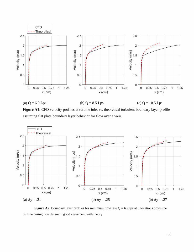
A1: Boundary Layer at Turbine Inlet

For the theoretical boundary layer, a crude assumption was made that the stream of water

flow of water along the weir face behaves like water over a flat plate, gives a Reynolds number

of 6.0, 6.15, and 6.30x106 respectively for each of the three cases. The theoretically turbulent

velocity profile is then (Munson,2012).

𝑢

𝑈𝑜≅ (

𝑦

𝛿)

1

7,

𝛿

𝑥=

0.37

(𝑅𝑒𝑥)15

x was taken as the length traveled by the water from the weir to the turbine entrance height, and

𝑈𝑜, the free velocity taken as the water velocity at the height of the inlet. Note that 𝛿 represents

the normal distance from a flat plate, so the assumption was made that is that there is little

variation

50

(a) Q = 6.9 Lps (b) Q = 8.5 Lps (c) Q = 10.5 Lps

Figure A1: CFD velocity profiles at turbine inlet vs. theoretical turbulent boundary layer profile

assuming flat plate boundary layer behavior for flow over a weir.

(a) Δy = .21 (b) Δy = .25 (b) Δy = .27

Figure A2. Boundary layer profiles for minimum flow rate Q = 6.9 lps at 3 locations down the

turbine casing. Resuls are in good agreement with theory.