energies

Article

A Novel Data Hierarchical Fusion Method for GasTurbine Engine Performance Fault Diagnosis

Feng Lu 1,2,*, Chunyu Jiang 1, Jinquan Huang 1, Yafan Wang 3 and Chengxin You 3

1 Jiangsu Province Key Laboratory of Aerospace Power Systems, College of Energy & Power Engineering,Nanjing University of Aeronautics and Astronautics, Nanjing 210016, Jiangsu, China;jcyjsxy1993@163.com (C.J.); jhuang@nuaa.edu.cn (J.H.)

2 Department of Mechanical and Industrial Engineering, University of Toronto, Toronto,ON M5S 3G8, Canada

3 Aviation Motor Control System Institute, Aviation Industry Corporation of China, Wuxi 214063, Jiangsu,China; yafwang@126.com (Y.W.); ycx0910@sina.com (C.Y.)

* Correspondence: lfaann@nuaa.edu.cn or fenglu@mie.utoronto.ca; Tel.: +86-25-8489-2406

Academic Editor: Chang Sik LeeReceived: 27 July 2016; Accepted: 11 October 2016; Published: 15 October 2016

Abstract: Gas path fault diagnosis involves the effective utilization of condition-based sensor signalsalong engine gas path to accurately identify engine performance failure. The rapid development ofinformation processing technology has led to the use of multiple-source information fusion for faultdiagnostics. Numerous efforts have been paid to develop data-based fusion methods, such as neuralnetworks fusion, while little research has focused on fusion architecture or the fusion of differentmethod kinds. In this paper, a data hierarchical fusion using improved weighted Dempster–Shafferevidence theory (WDS) is proposed, and the integration of data-based and model-based methodsis presented for engine gas-path fault diagnosis. For the purpose of simplifying learning machinetypology, a recursive reduced kernel based extreme learning machine (RR-KELM) is developedto produce the fault probability, which is considered as the data-based evidence. Meanwhile, themodel-based evidence is achieved using particle filter-fuzzy logic algorithm (PF-FL) by engine healthestimation and component fault location in feature level. The outputs of two evidences are integratedusing WDS evidence theory in decision level to reach a final recognition decision of gas-path faultpattern. The characteristics and advantages of two evidences are analyzed and used as guidelines fordata hierarchical fusion framework. Our goal is that the proposed methodology provides much betterperformance of gas-path fault diagnosis compared to solely relying on data-based or model-basedmethod. The hierarchical fusion framework is evaluated in terms to fault diagnosis accuracy androbustness through a case study involving fault mode dataset of a turbofan engine that is generatedby the general gas turbine simulation. These applications confirm the effectiveness and usefulness ofthe proposed approach.

Keywords: gas turbine; performance fault diagnosis; data fusion; extreme learning machine;evidence theory

1. Introduction

Gas turbine engine provides power for airplane, and its reliable operation plays an important rolein flight safety. Due to the complexity of structure and terrible work condition, gas turbine engine hasmore opportunity to break down [1]. Engine failures is generally divided into gas-path performancefault, vibration structure fault and auxiliary system fault, among which the performance fault causesmore maintenance costs and off-wing time [2]. Engine performance fault diagnosis is one of the keytechnologies to support advanced condition-based maintenance strategies and has received a wide

Energies 2016, 9, 828; doi:10.3390/en9100828 www.mdpi.com/journal/energies

Energies 2016, 9, 828 2 of 22

interest, with great potential to reduce engine maintenance costs and improve availability [3,4]. It isimportant to develop methodologies to improve the confidence of performance fault diagnosis for gasturbine engine using various kinds of available sensors.

Numerous approaches have been developed for engine health monitoring and gas-path faultdiagnosis, such as the model-based methods (nonlinear least square, and Kalman filter) [5–11],data-based methods (artificial neural networks, fuzzy logic, rough sets and decision tree, and expertsystems) [12–16]. The model-based method has been employed for engine gas-path fault diagnosissince 1970s, and the unmeasured component performance shifts are estimated from the residualsbetween the engine model outputs and sensed signals. Urban proposed a linearized model-basedmethod using nonlinear least square for gas-path analysis (GPA) [17], and it is the first time to producethe estimates of fault feature parameter from observable measurements. In order to improve estimationaccuracy, the state estimator based methods such as various Kalman filter (KF) and Particle filter (PF),are then introduced to engine health estimation. In the past twenty years, varieties of KF have beenwidely used for engine performance estimation and gas path fault diagnosis [7,8], and it is illustratedin Figure 1. In order to address engine nonlinearity in the health estimation, nonlinear model-basedmethods are developed using extended Kalman filter, unscented Kalman filter and PF [9,18,19]. Thesemodel-based methods performs well in some conditions, whereas their performance closely relieson the engine model precision [20,21]. It is difficult to obtain an accurate engine model to describethe dynamic and steady behavior at various operating conditions in whole flight envelope, and themodeling mismatch will bring false diagnosis.

Energies 2016, 9, 828 2 of 23

availability [3,4]. It is important to develop methodologies to improve the confidence of performance

fault diagnosis for gas turbine engine using various kinds of available sensors.

Numerous approaches have been developed for engine health monitoring and gas-path fault

diagnosis, such as the model-based methods (nonlinear least square, and Kalman filter) [5–11], data-

based methods (artificial neural networks, fuzzy logic, rough sets and decision tree, and expert

systems) [12–16]. The model-based method has been employed for engine gas-path fault diagnosis

since 1970s, and the unmeasured component performance shifts are estimated from the residuals

between the engine model outputs and sensed signals. Urban proposed a linearized model-based

method using nonlinear least square for gas-path analysis (GPA) [17], and it is the first time to

produce the estimates of fault feature parameter from observable measurements. In order to improve

estimation accuracy, the state estimator based methods such as various Kalman filter (KF) and

Particle filter (PF), are then introduced to engine health estimation. In the past twenty years, varieties

of KF have been widely used for engine performance estimation and gas path fault diagnosis [7,8],

and it is illustrated in Figure 1. In order to address engine nonlinearity in the health estimation,

nonlinear model-based methods are developed using extended Kalman filter, unscented Kalman

filter and PF [9,18,19]. These model-based methods performs well in some conditions, whereas their

performance closely relies on the engine model precision [20,21]. It is difficult to obtain an accurate

engine model to describe the dynamic and steady behavior at various operating conditions in whole

flight envelope, and the modeling mismatch will bring false diagnosis.

ŷ

State estimator

u

+-

y

Actual engine

SensorsEngine

control

Component

fault

Engine model

Engine health

condition

Figure 1. A model-based method for gas turbine engine health monitoring.

The data-driven method is another significant way to complete engine gas-path fault diagnosis.

Neural network (NN) is a well-known learning machine, and it is also an important data-based

method applied to detect and isolate engine component and sensor faults [13]. Variants of the NNs

are fulfilled with the goal of the smallest empirical risk, and the dimension disaster or over-fitting

might occur due to a large number of samples required [22,23]. Support vector machine (SVM) is

proposed on the basis of the minimum structural risk in the last twenty years, and this statistical

learning approach has strictly mathematical deduction [24,25]. The SVM is employed to monitor gas

turbine performance degradation, and it is proved to be superior to the basic NN with classification

capability and generalization performance regards [26]. Kernel extreme learning machine (KELM) is

recently developed from the NNs and SVM with kernel transformation, and it has less coefficients

need to be calculated in the training process simple topology [27]. The KELM is used to feature

extraction, pattern recognition and fault diagnosis.

However, the original KELM is lack of sparseness, which makes its topological structure

complexity grow with sample size. It affects the real-time capability of the KELM. Thus choosing

suitable samples to realize sparseness of KELM plays a key role in training KELM in the cases of

Figure 1. A model-based method for gas turbine engine health monitoring.

The data-driven method is another significant way to complete engine gas-path fault diagnosis.Neural network (NN) is a well-known learning machine, and it is also an important data-basedmethod applied to detect and isolate engine component and sensor faults [13]. Variants of the NNsare fulfilled with the goal of the smallest empirical risk, and the dimension disaster or over-fittingmight occur due to a large number of samples required [22,23]. Support vector machine (SVM) isproposed on the basis of the minimum structural risk in the last twenty years, and this statisticallearning approach has strictly mathematical deduction [24,25]. The SVM is employed to monitor gasturbine performance degradation, and it is proved to be superior to the basic NN with classificationcapability and generalization performance regards [26]. Kernel extreme learning machine (KELM) isrecently developed from the NNs and SVM with kernel transformation, and it has less coefficients needto be calculated in the training process simple topology [27]. The KELM is used to feature extraction,pattern recognition and fault diagnosis.

Energies 2016, 9, 828 3 of 22

However, the original KELM is lack of sparseness, which makes its topological structurecomplexity grow with sample size. It affects the real-time capability of the KELM. Thus choosingsuitable samples to realize sparseness of KELM plays a key role in training KELM in the cases oflarge-scale datasets. At the aim of simplified KELM topology, some studies on pruning techniqueshave been done [28,29], but these variations focus on structure sparseness not data sparseness. Sincethere is a one-to-one correspondence between a hidden node and a sample In KELM, it is possible toachieve sparsity in terms of training data. A sparse ELM (S-ELM) algorithm is proposed to greatlyreduce the storage space and forecasting time, and it replacing the equality constraints by inequalityconstraints [30]. Then a fast sparse approximation scheme of extreme learning machine (FSA-ELM) isproposed [31], and it has the features of low complexity and sparse solution. FSA-ELM defines onebasis function for each sample in the training set and iteratively builds the decision function by addingone basis function from the kernel-based dictionary. However, the constraints brought by samplesthat are not selected to the decision function are not considered, and the problem of weight betweenthe topology sophistication and prediction accuracy rises up. For the purposes of simplifying KELMtopology with less reduction of accuracy, the RR-KELM is proposed on the basis of the FSA-ELM usinga reduced technique in this paper.

When the in-flight performance fault diagnosis for gas turbine engine is concerned, the confidencerequirements of fault pattern recognition increases. The sensor fusion technologies using learningmachine are developed, such as the integration of multiple types NNs, or combination of NN and fuzzylogic [32,33]. The essence of these fusion approaches are the data-based ones, and aero-thermodynamiccharacteristics of gas turbine engine is not taken into account [34]. These data-based sensor fusionmethods would be still failed to new fault modes due to the lack of very training samples. In thispaper, the combination of model-based and data-driven using weighted Dempster–Shaffer evidencetheory (WDS) with different feature information in data hierarchical fusion framework is developed.Our main objective in this work is to develop a data hierarchical fusion framework to improve theperformance of in-flight gas-path fault diagnosis. One model-based evidence is brought by the PF-FLalgorithm in feature level, and the other data-based evidence one produced by the RR-KELM. Afinal decision of performance fault pattern for airplane engine is achieved from two evidences usinginformation fusion scheme in decision level. To confirm the effectiveness of the proposed methodology,turbofan engine data from a general gas turbine simulation are applied to carry out experiments. Fromthese reports, it is easily got that the data hierarchical fusion method has satisfactory confidence ofperformance fault diagnosis.

The paper is organized as follows. The problem formulation is given, and the RR-KELM isproposed to produce one data-based evidence of gas-path fault diagnosis in feature level in Section 2.The model-based method using PF-FL is then discussed to produce another evidence, and the WDS anddata hierarchical fusion mechanism for gas-path fault diagnosis are developed in Section 3. Section 4shows the simulation and analysis, and it indicates the performance of the data hierarchical fusionframework using the WDS is improved in respects of fault diagnosis accuracy and robustness. Section 5draws a conclusion and discussed future research directions.

2. Data-Based Fault Diagnosis Using the RR-KELM

Gas turbine engine is a complex mechanical system, and in this paper a two-spool mixing-exhaustturbofan engine is studied. The engine mainly includes the following components: Inlet, Fan,Compressor, Combustor, High-Pressure Turbine (HPT), Low-Pressure Turbine (LPT), Bypass, MixingChamber and Nozzle [35,36]. Figure 2 gives the schematic representation of the examined gas turbineengine. The airflow is driven into the fan after through an inlet. It is then separated into two streamsbefore the compressor: one stream passes through the annular bypass duct and the other through theengine core. Fuel is sprayed into the combustor, mixed with the air from the compressor and burned toproduce hot gas to drive the turbines. There are two spools, through which the high pressure turbine(HPT) drives compressor, and the low pressure turbine (LPT) drives fan. The gas leaves the LPT and

Energies 2016, 9, 828 4 of 22

mixed the air from the bypass in the mixing chamber. The mixed gas is guided into the nozzle at last,and it has a variable throttle area.Energies 2016, 9, 828 4 of 23

22 3 43 6

Inlet Fan Compressor HPT LPT

Combustor

Mixing Chamber NozzleBypass

SE1 SE2 SE3 SE4

Figure 2. Schematic representation of gas turbine engine.

Engine gas-path fault results from fouling, leakage, erosion, corrosion, seal damage, foreign and

domestic objective damage, and hot end components damage, and it becomes serious with the

increase of usage cycle number. The deviation of health parameter is called fault feature parameter,

which is used to quantitatively represent engine gas-path fault modes. The fault feature parameters

include the deviations of fan efficiency SE1, compressor efficiency SE2, HPT efficiency SE3 and LPT

efficiency SE4, which cannot be directly measured. As we know, gas-path fault causes the sensed

parameters change, then the measurement deviation could be used to calculate fault feature

parameter. The engine measurements include low-pressure spool speed NL, high-pressure spool speed

NH, fan outlet temperature T22, fan outlet pressure P22, compressor outlet temperature T3, compressor

outlet pressure P3, LPT inlet temperature T43, and LPT outlet temperature T6. The elements of control

vector are fuel flow Wf and nozzle area A8, which determine the engine operating conditions. In this

section, the RR-KELM algorithm is proposed and employed to achieve the classification of gas-path

fault modes, and the fault mode identification result is served as data-based evidence.

2.1. KELM

The KELM is developed from the ELM with the kernel transformation method, and it brings

better generalization than the ELM in the most applications due to the kernel transformation to the

feature space [27,37]. Assume the training set of KELM {( , ) | , , 1,2, , }n

i i i iy y i N x x R R .

The learning problem of KELM is to search an optimal function F: xi→yi, and it is presented by

i iF yx . Once an activation function gi() and hidden neuron number L is given, the function F() is

expressed

1

( ) ( ) ( ) L

T

i i

i

y F g

x x G x β (1)

where β = [β1, β2, …, βL]T is output weights from the hidden neurons to output nodes, and G(x) =

[g1(x), g2(x), …, gL(x)]T is output vector of the hidden neurons corresponding to input x. For the general

ELM optimization theory, it is to search the optimal output weights to produce the minimum of

empirical risk and structural risk, and the risk function is TR C G y . Thus the learning

problem of ELM is converted

2 2

21

1min

2 2

. . ( ) , 1,2, ,

N

i

i

T

i i i

C

s t y i N

G x

(2)

where the penalty factor C is a trade-off between output weights norm and fitting error, and the slack

variable i implies the differences between predicted and actual value. Given the output vector is y

= [y1, y2, …, yN]T, the optimal output weight of ELM in Equation (2) is written

Figure 2. Schematic representation of gas turbine engine.

Engine gas-path fault results from fouling, leakage, erosion, corrosion, seal damage, foreign anddomestic objective damage, and hot end components damage, and it becomes serious with the increaseof usage cycle number. The deviation of health parameter is called fault feature parameter, which isused to quantitatively represent engine gas-path fault modes. The fault feature parameters includethe deviations of fan efficiency SE1, compressor efficiency SE2, HPT efficiency SE3 and LPT efficiencySE4, which cannot be directly measured. As we know, gas-path fault causes the sensed parameterschange, then the measurement deviation could be used to calculate fault feature parameter. Theengine measurements include low-pressure spool speed NL, high-pressure spool speed NH, fan outlettemperature T22, fan outlet pressure P22, compressor outlet temperature T3, compressor outlet pressureP3, LPT inlet temperature T43, and LPT outlet temperature T6. The elements of control vector are fuelflow Wf and nozzle area A8, which determine the engine operating conditions. In this section, theRR-KELM algorithm is proposed and employed to achieve the classification of gas-path fault modes,and the fault mode identification result is served as data-based evidence.

2.1. KELM

The KELM is developed from the ELM with the kernel transformation method, and it bringsbetter generalization than the ELM in the most applications due to the kernel transformation to thefeature space [27,37]. Assume the training set of KELM ℵ = {(xi, yi)|xi ∈ Rn, yi ∈ R, i = 1, 2, . . . , N}.The learning problem of KELM is to search an optimal function F: xi→yi, and it is presented byF (xi) ≈ yi. Once an activation function gi() and hidden neuron number L is given, the function F()is expressed

y = F(x) =L

∑i=1

βigi(x) = G (x)T β (1)

where β = [β1, β2, . . . , βL]T is output weights from the hidden neurons to output nodes,and G(x) = [g1(x), g2(x), . . . , gL(x)]T is output vector of the hidden neurons corresponding to input x.For the general ELM optimization theory, it is to search the optimal output weights to produce theminimum of empirical risk and structural risk, and the risk function is R = ||β|| + C||GTβ− y||.Thus the learning problem of ELM is converted

minβ

12 ||β||2

2 +C2

N∑

i=1ε2

i

s.t. GT(xi)β = yi − εi, i = 1, 2, . . . , N(2)

Energies 2016, 9, 828 5 of 22

where the penalty factor C is a trade-off between output weights norm and fitting error, and the slackvariable εi implies the differences between predicted and actual value. Given the output vector isy = [y1, y2, . . . , yN]T, the optimal output weight of ELM in Equation (2) is written

β = G(

1C

IN + GTG)−1

y (3)

Comparing to the basic ELM, a regularization term 1C IN is added to the KELM. Besides, the kernel

transformation k(xi, xj), namely a mapping from input space to feature space, replaces an explicitactivation function in the hidden layer of the ELM

Ki,j = GT (xi) ·G(xj)= k

(xi, xj)

k(xi, xj) = exp(−γ||xi − xj||2)(4)

where the kernel parameter γ is the kernel distribution width. The KELM function in Equation (1) canbe calculated as follows

F(x) = GT(x)β = GTG( 1C IN + GTG)

−1y = k(x)α

α =(

1C IN + K

)−1y

(5)

where α is the output weight of the KELM. It is noted that the number of hidden nodes in KELMequals to the training sample count. When it comes to the large-scale datasets, especially in the cases ofperformance fault diagnosis at various operating conditions in whole flight envelope, the topologicalstructure of KELM might be redundant. Then the sparsity of KELM is emerged, and it affects not onlyreal-time calculation but also the generalization performance for gas-path fault diagnosis.

A fast sparse approximation (FSA) scheme is developed to the problem that the model scalegrows hazard as sample size increase [31]. Provided a kernel function k(x, xi) is one basis functionfor each sample xi in the training set, a set of basis functions D = {k(x, xi)|i = 1, · · · , N} is called akernel-based dictionary. FSA-ELM is a greedy algorithm which iteratively builds the decision functionby adding one basis function from the kernel-based dictionary at one time. The key of FSA-ELM isto select the basis function. The FSA-ELM starts from an empty index set P = ∅ and a full index setQ = {1, 2, · · · , N}, and selects a new basis function k(x, xs) from the set {k(x, xi)|i ∈ Q}. It providesinsights into simplifying the topological structure of KELM.

2.2. RR-KELM

Given a random small-scale subset Xs = {xi}si=1 is selected from the original N data points

X = {xi}Ni=1 with s � N using this reduced technique, and the learning problem Equation (2) is

regulated for the reduced dataset as follows

minα

{Ls =

12

αT KSSα +C2

N

∑i=1

[yi −∑j∈S

αjk(xj, xi)]2

}(6)

where KSS(i, j) = k(xi, xj), i, j ∈ S. Since the number of training sample is s less than that of basicKELM, the hidden neuron count is s and the topology of learning machine is simplified compared tothe original KELM topology. The optimization target keeps the N constraints of the whole dataset, andit helps to enhance the generalization performance.

Let ∂Ls∂α = 0 in Equation (6), we have(

KSS/C + KSNKTSN

)α = KSNy (7)

Energies 2016, 9, 828 6 of 22

where KSN(i, j) = k(xi, xj), i ∈ S, j = 1, 2, . . . , N. Note that this reduced technique might producelower testing accuracy than basic K-ELM due to randomly selecting the subset of training data.

On the other hand, FSA-ELM presented a strategy of selecting the optimal kernel functions.Nevertheless, the defect of FSA-ELM is that the contribution of the rest non-selected data is notconsidered to the output weights. Therefore, the RR-KELM is proposed from the FSA-ELM using thereduced technique. The reduced training samples technique that includes the whole N constraintsinformation is discussed, and the iterative calculation strategy is combined in RR-KELM.

2.2.1. Strategy of Selecting the Reduced Subset

When the kernel function of a new basis k(x, xi) is determined at the (n + 1)-th iteration,the optimization target function Equation (6) can be reformulated as

minαs

{Ls =

12 αT (KSS/C + USS) α− αTKSNy

}min

αs

{Ls =

12

[αT

n αi

] ([ KSS/C ki

kiT k(xi, xi)/C

]+

[Uss uiuT

i Uii

]) [αn

αi

]−[

αTn αi

] [ KSNKiN

]y

} (8)

where USS = KSNKTSN , and the output weights vector αn = [α1, α2, · · · , αn]

T at the n-thiteration. The expressions follow ki = [k(xs1, xi), k(xs2, xi) , · · · , k(xsn, xi)]

T/C , s1, s2, · · · , sn ∈ S,KiN = [k(x1, xi) , k(x2, xi), · · · , k(xN , xi)]

T , ui = KSNKTiN , Uii = KiNKT

iN . The candidates of basisfunction have little effects on the selected training samples, and the output weights in αn are fixed andEquation (8) is further simplified

minαi

{Ls =

(k(xi, xi)/C + Uii)

2αi

2 + riαi

}(9a)

ri =

−yi , n = 0(ki

T+ uT

i

)αn − yi, n > 0

(9b)

where yi = KiNy. Thus, we select the index s from Q into S based on the following criterion

s = argmini∈Q

(− (ri)

2

2(k(xi ,xi)/C+kiTki)

)(10)

The stopping condition of iteration is

max(∣∣rQ∣∣) < δ or n > M (11)

where δ is a small positive constant, n is total number of selected basis functions, and M is themaximum subset.

2.2.2. Iterative Computation of the Kernel Matrix Inversion

Let R = (KSS/C + USS)−1, the solution of Equation (11) is

αns = RKSNy (12)

A new sample xi is picked up at the (n + 1)-th iteration, and the expression is as follows

Rn+1 =

[[Kss/C kT

iki k(xi, xi)/C

]+

[Uss uT

iui Uii

]]−1

(13)

Energies 2016, 9, 828 7 of 22

Theorem 1. Given an arbitrary invertible matrix A and matrices D, V, U, the following expression holds[A UV D

]−1

=

[A−1 + A−1U(D− VA−1U)

−1VA−1 −A−1U(D− VA−1U)−1

−(D− VA−1U)−1VA−1 (D− VA−1U)

−1

](14)

Let β = Rn(ki + ui), λ = (k(xi, xi)/C + Uii − (kiT+ ui

T)β), and then Equation (13) is rewrittenusing Theorem 1

Rn+1 =

[Rn 00 0

]+ λ

[β

−1

] [βT −1

](15)

Combining the iterative computation of the kernel matrix inversion with the strategy of selectingreduced subset, the proposed RR-KELM is described in the following.

Algorithm RR-KELM

(1)Initialization: inputs includes kernel function k(xi, xj), regularization parameterC, training set {(xi, yi), i = 1, 2, . . . , N}; Output contains the output weights α

computed after the last iteration.

(2)Let S = ∅, Q = {1, 2, . . . , N}, n = 0, and define a small positive constant δ and apositive integer M.

(3) If Q = ∅ or max(∣∣rQ

n∣∣) < δ or n > M stop the iteration.

(4) s = argmini∈Q

(− (ri)

2

2(kii/C+kiTki)

).

(5) Compute Rn+1 and αn+1s separately from Equations (15) and (12).

(6) Q = Q− {s} , S = S + {s}.(7) rQ(i) =

(ki

T+ uT

i

)αs − yi, i ∈ Q.

(8) n = n + 1, go to Step 3.

As far as engine gas-path fault diagnosis, the RR-KELM input for is a 9-element vector includingthe engine parameters Wf, NL, NH, T22, P22, T3, P3, T43 and T6. The RR-KELM’s output is a 10-elementvector of fault probability, and each element related to one engine gas-path fault pattern given inTable 1. The i-th fault mode is identified as the i-th element of fault probability vector is the maximumand more than 0.5, and the fault probability vector is used as the decision of data-based evidence.

Table 1. Fuzzy logic rules for engine gas-path fault diagnosis.

Rule No.If Then

Fault Component∆SE1 ∆SE2 ∆SE3 ∆SE4 Fault Mode

1 High Low Low Low F1 Fan2 Low High Low Low F2 Compressor3 Low Low High Low F3 HPT4 Low Low Low High F4 LPT5 High High Low Low F5 Fan and Compressor6 High Low High Low F6 Fan and HPT7 High Low Low High F7 Fan and LPT8 Low High High Low F8 Compressor and HPT9 Low High Low High F9 Compressor and LPT

10 Low Low High High F10 HPT and LPT

3. Data Hierarchical Fusion for Engine Gas-Path Fault Diagnosis

Generally speaking, there are three kinds of data fusion structure, namely data-level fusion,feature-level fusion and decision-level fusion. Data-level fusion is the lowest layer information, whichdirectly integrates multiple sensor data. A data-level fusion scheme is applied to degradation modeling

Energies 2016, 9, 828 8 of 22

and prognostic analysis for turbofan engine [32]. The original measurements are treated by extractingfault feature information, and then the information is integrated called feature-level fusion for faultdiagnosis [33]. A fuzzy-based method in feature-level fusion is presented for gas turbine fault detectionand identification [38]. The intermediate decision of each module combined for final decision in thetopmost layer is denoted by decision-level fusion. The Dempster–Shaffer evidence theory (DS) isone of the most common fusion methods since it is simple and easy for implement. The DS hasbeen applied for engine anomaly detection and vibration fault diagnosis [39]. The WDS in the datahierarchical fusion mechanism and the integration of two different kinds of evidences are discussedfor engine gas-path fault diagnosis in this section. The fault mode index by the method-based evidenceand fault mode probability by the data-based evidence are combined in the decision layer in thefusion framework.

3.1. Model-Based Fault Diagnosis Using PF-FL Method in Feature Layer

The nonlinear model-based method using PF-FL for engine gas-path fault diagnosis completes bytwo steps: fault feature parameter estimation and fault identification. The PF algorithm is served asa state estimator to calculate the component performance deviations from their normal values. Thedeviations of fault feature parameters are then fed to the fuzzy logic system for fault mode recognition.The fault mode index is computed by the PF-FL and used as the model-based evidence.

Considering air flow mass, power and momentum conservation laws, a general gas turbineengine simulation is designed [35]. The characteristic maps of engine rotating components describeaero-thermodynamic relationships of component inputs and outputs in the engine simulation [36].The data of engine design operation and component maps are loaded to the general simulation forobtaining a turbofan engine component level model (CLM) [40]. The nonlinear mathematical model ofthe engine is given by

xk+1 = f (xk, uk) + wkyk = g(xk, uk) + vk

(16)

where k is the time index, y is the 8-element measured output, x is the 6-element augmented statevariable, and u is the 2-element control input. The noise terms w and v represent process uncertaintyand measurement uncertainty in the model. Since the PF is based on sequential Monte Carlosampling theory and aimed to state estimation of nonlinear and non-Gauss system [41], it is especiallysuitable to gas turbine engine. Hence, the PF algorithm is employed to the estimation of engine faultfeature parameters.

Let x0:k = {x0, · · · , xk} denote the series of the augmented state vector [NL, NH, SE1, SE2, SE3, SE4]T,and y1:k = {y1, · · · , yk} denote the series of measurement vector [NL, NH, T22, P22, T3, P3, T43, T6]T.Give the probability density function (PDF) of the prior condition is p(x0), and the posterior PDFp(x0:k|y1:k) is characterized by a set of weighted random samples

{xi

0:k, wik}N

i=1, wherein N is particlenumber. The particle set

{xi

0:k; i = 0, · · · , N}

is related to the weight{

wik; i = 0, · · · , N

}, and the PDF

at time k is approximated by

p(x0:k|y1:k) ≈ ∑N1 wi

kδ(x0:k − x0:ki)

∑N1 wi

k = 1(17)

The case for Monte Carlo sampling is to generate particles from the posterior PDF p(x0:k|y1:k),but it is unavailable directly. Then the importance sampling distribution function q(x0:k|y1:k) isexpressed before sampling

q(xk|x0:k−1, z1:k) = q(xk|xk−1, zk)

q(xik

∣∣∣xik−1, zk) = p(xi

k

∣∣∣xik−1)

(18)

The i-th particle weight wik can be approximated by

wik ∝

p(x0:k |y1:k )

q(x0:k |y1:k )∝

p(yk∣∣xi

k )p(xik

∣∣∣xik−1 )p(xi

0:k−1 |y1:k−1 )

q(xik

∣∣∣xi0:k−1, y1:k )q(xi

0:k−1 |y1:k−1 )= wi

k−1

p(yk∣∣xi

k )p(xik

∣∣∣xik−1 )

q(xik

∣∣∣xi0:k−1, y1:k )

(19)

Energies 2016, 9, 828 9 of 22

The importance weights is normalized

wik = wi

k/N

∑i=1

wik (20)

There is a problem of basic PF algorithm that more particles have negligible weights after severaliterations, and it indicates that particle generation degeneracy emerges and a large computationaleffort for updating particle becomes meaningless [18]. Then, importance re-sampling is added andeach particle is assigned by the weight wi

k = 1/N whenever the effective particles number Ne f f is lessthan a threshold value Nth

Ne f f =1

N∑

i=1

(wi

k)2

< Nth (21)

All particles have almost the same significance if Neff is close to the threshold Nth. The estimatesof fault feature parameters (SE1, SE2, SE3, and SE4) are obtained by the PF, which are then used forfault location in the feature level. The fault feature estimates by the PF are quantitative representation,and it cannot directly lead to a fault mode decision and utilized for model-based evidence. Fuzzy logicis an approach based on “degrees of truth” rather than the usual “true or false” [33], and it is appliedto recognize engine gas-path fault pattern with continuous fault mode membership. The estimatesof fault feature parameter are assigned to fuzzy logic system to acquire the fault mode index thatrepresents performance fault type.

The fuzzy logic rules of fault mode classification give the mapping of fault feature parameters tofault mode index, and are shown in Table 1. There are four key rotating components (fan, compressor,HPT and LPT), and each component relates to two linguistic variables (Low and High) [42]. Thelinguistic variable of engine operating state is Low as fault feature parameter bias less than 1%, andHigh as it falls into (1%, 5%). The number of fault pattern studied is totally ten, wherein the number ofsingle component failure is four, and double component failure number is six.

As seen in Table 1, fan fault mode in the fuzzy rule is defined that SE1 is high, and SE2, SE3, andSE4 are low. The membership function of fuzzy logic is Gauss function. The fuzzy inputs are theestimates of fault feature parameters, and the outputs are fault mode index. Gravity model is used inthe defuzzifier process, and the fault mode index is calculated as follows

o∗ =r

o oB(o)dyr

o B(o)dy(22)

where o* is the exact value of fault mode membership, B( ) is membership function, and o is oneelement in the fuzzy set.

Take fuzzy logic on fan as an example, the membership functions of fault feature parameter SE1and Fan fault mode are shown in Figure 3a,b, respectively. The membership functions for the rest faultfeature parameters SE2, SE3, and SE4 and their fault modes are formulated in a similar way.

Engine performance fault classification using fuzzy logic is conducted as follows: the estimates offault feature parameter are converted to the linguistic variables in the fuzzy subset using the Gaussmembership. The linguistic variables corresponding to the outputs are obtained by the fuzzy logicrules. Fuzzy distribution is calculated in the inference machine, and the fault mode index is exactlycalculated by defuzzifing. The decision of engine gas-path fault pattern is recognized using fault modeindex in the feature layer, and this index is also used as the model-based evidence results for furtherfault diagnosis in the decision level.

Energies 2016, 9, 828 10 of 22Energies 2016, 9, 828 10 of 23

(a) (b)

Figure 3. (a) Membership function for SE1; and (b) membership function for fan fault mode.

3.2. Data Hierarchical Fusion Diagnosis Using Improved Weighted DS Evidence Theory

The information reasoning and fusion can be done by DS evidence theory, whereas this method

might fail in some cases of information incomplete or uncertainty [43,44]. In order to improve the

confidence of DS evidence theory, the WDS is developed and applied to integrate the model-based

evidence E1 and data-based evidence E2 to reach a final decision of gas-path fault diagnosis. Let ϴ be

an elements set of discernment frame, and it means all performance fault modes, namely, ϴ = {F1, F2,

F3, F4, F5, F6, F7, F8, F9, F10}. The set map m: 2ϴ -> [0,1] is a basic probability assignment function (BPAF)

in the frame ϴ, and it follows

( ) 0; ( ) 1A

m m A

(23)

where the proposition A, A1, and A2 are the subsets of ϴ, is empty set, and the basic confidence

m(A) is the confidence level of the proposition A. When two evidences E1 and E2 are concerned in the

frame ϴ, their BPAFs are m1 and m2, respectively. The propositions A1 and A2 are corresponding to

the evidences E1 and E2, and the propositions A relates to the combination of the former evidences in

the frame ϴ. The BPAF of the fusion based on two evidences is expressed as follows

1 2

1 1 2 2( ) ( )

( )1

0

A A A

i

i

m A m A

m A AK

A

(24)

where the parameter

1 2

1 1 2 2( ) ( )A A

K m A m A

represents the conflicts between two evidences. The

inconsistence level of two evidences increases as the larger K. It has more opportunity to reach a false

conclusion once the evidence conflict becomes seriously. The fault feature and fault diagnostic

mechanism by the data-based and model-based evidences are different for engine gas-path system,

and the WDS fusion method relies on adaptive fused BPAF of two evidences. The confusion matrix

in the WDS is used to compute the confidence of each evidence, and the evidence weight in the fused

BPAF is tuned to the evidence confidence.

The confusion matrices corresponding to the model-based and data-based evidences are

separately expressed V1 and V2

1,1 1,2 1,10

2,1 2,2 2,10

10,1 10,2 10,10

, ,

1,2

/

t

i j i j i

v v v

v v vt

v v v

v n n

V (25)

where ni,j is the sample number of the fault mode i misdiagnosis to fault mode j, and ni is the total

sample number in fault mode i. The element vi,j is the false diagnosis percentage that the fault mode

Figure 3. (a) Membership function for SE1; and (b) membership function for fan fault mode.

3.2. Data Hierarchical Fusion Diagnosis Using Improved Weighted DS Evidence Theory

The information reasoning and fusion can be done by DS evidence theory, whereas this methodmight fail in some cases of information incomplete or uncertainty [43,44]. In order to improve theconfidence of DS evidence theory, the WDS is developed and applied to integrate the model-basedevidence E1 and data-based evidence E2 to reach a final decision of gas-path fault diagnosis. Letθ be an elements set of discernment frame, and it means all performance fault modes, namely,θ = {F1, F2, F3, F4, F5, F6, F7, F8, F9, F10}. The set map m: 2θ -> [0,1] is a basic probability assignmentfunction (BPAF) in the frame θ, and it follows

m(∅) = 0; ∑A⊂Θ

m(A) = 1 (23)

where the proposition A, A1, and A2 are the subsets of θ, ∅ is empty set, and the basic confidencem(A) is the confidence level of the proposition A. When two evidences E1 and E2 are concerned in theframe θ, their BPAFs are m1 and m2, respectively. The propositions A1 and A2 are corresponding to theevidences E1 and E2, and the propositions A relates to the combination of the former evidences in theframe θ. The BPAF of the fusion based on two evidences is expressed as follows

m(A) =

∑

A1∩A2=Am1(A1)m2(A2)

1−K Ai 6= ∅0 Ai = ∅

(24)

where the parameter K = ∑A1∩A2=∅

m1(A1)m2(A2) represents the conflicts between two evidences.

The inconsistence level of two evidences increases as the larger K. It has more opportunity to reach afalse conclusion once the evidence conflict becomes seriously. The fault feature and fault diagnosticmechanism by the data-based and model-based evidences are different for engine gas-path system,and the WDS fusion method relies on adaptive fused BPAF of two evidences. The confusion matrix inthe WDS is used to compute the confidence of each evidence, and the evidence weight in the fusedBPAF is tuned to the evidence confidence.

The confusion matrices corresponding to the model-based and data-based evidences are separatelyexpressed V1 and V2

Vt =

v1,1 v1,2 · · · v1,10

v2,1 v2,2 · · · v2,10...

.... . .

...v10,1 v10,2 · · · v10,10

(t = 1, 2)

vi,j = ni,j/ni

(25)

where ni,j is the sample number of the fault mode i misdiagnosis to fault mode j, and ni is the totalsample number in fault mode i. The element vi,j is the false diagnosis percentage that the fault mode

Energies 2016, 9, 828 11 of 22

i is mis-recognized as the mode j by one evidence. The diagonal elements of the confusion matrixindicate the correct identification rate of every fault mode. In order to increase the effect of evidencethat produces less incorrect recognition, the weighted coefficient is introduced

W(A) =k · R3(A)

∑A⊂Θ

R3(A)(26a)

R(Fj) =vj,j

10∑

i=1vi,j

(26b)

where the coefficient R(Fj) depicts the reliability of one evidence for fault diagnostics in the fault modej. rank is the descending sort number of basic probability assignment in each fault mode, and smallerseries number rank implies larger confidence of the evidence. k is 2 as the series number rank equals 1,2 or 3, otherwise k is 1. The adaptive fused BPAF m*(A) is presented as follows

m∗(A) =

∑

A1∩A2=AWm1 (A1)Wm2 (A2)

1−K Ai 6= ∅0 Ai = ∅

(27a)

Wmi (A) =W(A) ·mi(A)

∑A⊂Θ

W(A) ·mi(A)(27b)

where Wmi() is the weighted BPAF of the Ei, and K = ∑A1∩A2=∅

Wm1(A1)Wm2(A2).

The WDS for fault diagnosis is presented in detail as follows

Step 1: Initiate the confusion matrices V1 and V2, which are calculated from training samplesusing Equation (25).

Step 2: Load the confusion matrices V1 and V2 to calculate the reliability parameters for twoevidences using Equation (26b).

Step 3: Calculate the weighted BPAF of two evidences.If two evidences E1 and E2 are conflictedCalculate weighted coefficients for E1 and E2 using Equation (26a)Calculate the weighted BPAF for E1 and E2 using Equation (27b)ElseWm1(A1) = m1(A1) and Wm2(A2) = m1(A2)Step 4: Combine two evidences to reach adaptive fused BPAF using Equation (27a).Step 5: Obtain turbofan engine gas-path fault pattern which is corresponded to the largest m*(F).

A data hierarchical fusion framework using the WDS is designed to increase the confidence ofgas-path fault diagnostics for turbofan engine, and it is shown in Figure 4. The PF-FL is utilized toreach the model-based evidence for gas-path fault diagnosis, and it runs parallel with the RR-KELM inthe hierarchical fusion framework. The sensed data along the engine gas path used for fault diagnosis,like speeds, temperatures, pressures, vary with the power condition and ambient conditions. In orderto extend the designed approach to the whole flight envelope and decrease the negative effects ofvarious physical parameters magnitude difference, the aero-thermodynamic parameters are correctedand normalized before the fault diagnosis applications. Details of correction and normalization can befound in Reference [36].

Energies 2016, 9, 828 12 of 22Energies 2016, 9, 828 12 of 23

Fault feature

parameter estimationFault classification

Fault mode index and

membership

Fault mode

probability

Fault diagnosis by

evidence 1

Fault diagnosis by

evidence 2

Fault diagnostic

reliability by PF-Fuzzy

Fault diagnostic

reliability by RR-KELM

Weighted

coefficient

Weighted

coefficient

m1 m2W1 W2

Weighted DS evidences fusion

Wm1 Wm2

Engine gas-path fault diagnosis decision

Model- based

evidence

Data-based

evidence

Engine sensor (Wf, NL, NH ,T22, T33, P3, P43, T5 and T6)

Gas-path fault

database

Similarity transformation and normalization

V1 V2

Figure 4. Data hierarchical fusion framework for engine gas-path fault diagnosis.

The engine health parameter deviations are estimated and used as fault feature parameters by

fuzzy logic to produce fault mode index. Meanwhile, the RR-KELM is implemented to produce fault

mode probability from the engine measurements. The confusion matrices and weighted coefficients

are the prior information calculated from engine gas-path fault database. With the help of this prior

information, the decisions of evidences about fault mode are obtained using the model-based and

data-based methods, and then are combined to reach an engine fault pattern recognition decision by

the WDS in the data hierarchical fusion framework.

4. Simulation and Analysis

The proposed gas-path fault diagnosis method is evaluated on the general gas turbine engine

simulation using MATLAB software. The developed CLM of turbofan engine takes the place of an

actual engine, and the sampling rate of CLM equals to 50 Hz [40,45]. The hardware of computer used

for simulation is configured CPU i5-5200U @ 2.20 GHz and RAM 4 GB. The involved engine

component fault patterns have been shown in Table 1, and sensor and actuator faults are not

considered. Eight measurements are employed for gas-path fault diagnosis, and their standard

deviations and CLM modeling errors are shown in Table 2. Gaussian noise v with standard

deviations given in Table 2 is added to the measured parameters, and the independent system noise

and measured noise follow w~N(0,Q) and v~N(0,R), wherein Q = 0.16 × 10−4I6×6.

Table 2. Gas turbine engine measurement numerical characteristics.

Measurement Acronyms Nominal Value Standard Deviation Modeling Errors

Low pressure spool speed NL 1 0.0075 0.0015

High pressure spool speed NH 1 0.0075 0.0015

Fan outlet temperature T22 1 0.0100 0.0020

Fan outlet pressure P22 1 0.0075 0.0015

Compressor outlet temperature T3 1 0.0100 0.0020

Compressor outlet pressure P3 1 0.0075 0.0015

HPT outlet temperature T43 1 0.0100 0.0020

LPT outlet temperature T6 1 0.0100 0.0020

Figure 4. Data hierarchical fusion framework for engine gas-path fault diagnosis.

The engine health parameter deviations are estimated and used as fault feature parameters byfuzzy logic to produce fault mode index. Meanwhile, the RR-KELM is implemented to produce faultmode probability from the engine measurements. The confusion matrices and weighted coefficientsare the prior information calculated from engine gas-path fault database. With the help of this priorinformation, the decisions of evidences about fault mode are obtained using the model-based anddata-based methods, and then are combined to reach an engine fault pattern recognition decision bythe WDS in the data hierarchical fusion framework.

4. Simulation and Analysis

The proposed gas-path fault diagnosis method is evaluated on the general gas turbine enginesimulation using MATLAB software. The developed CLM of turbofan engine takes the place of anactual engine, and the sampling rate of CLM equals to 50 Hz [40,45]. The hardware of computerused for simulation is configured CPU i5-5200U @ 2.20 GHz and RAM 4 GB. The involved enginecomponent fault patterns have been shown in Table 1, and sensor and actuator faults are not considered.Eight measurements are employed for gas-path fault diagnosis, and their standard deviations andCLM modeling errors are shown in Table 2. Gaussian noise v with standard deviations given in Table 2is added to the measured parameters, and the independent system noise and measured noise followw~N(0,Q) and v~N(0,R), wherein Q = 0.16 × 10−4I6×6.

Table 2. Gas turbine engine measurement numerical characteristics.

Measurement Acronyms Nominal Value Standard Deviation Modeling Errors

Low pressure spool speed NL 1 0.0075 0.0015High pressure spool speed NH 1 0.0075 0.0015

Fan outlet temperature T22 1 0.0100 0.0020Fan outlet pressure P22 1 0.0075 0.0015

Compressor outlet temperature T3 1 0.0100 0.0020Compressor outlet pressure P3 1 0.0075 0.0015

HPT outlet temperature T43 1 0.0100 0.0020LPT outlet temperature T6 1 0.0100 0.0020

Energies 2016, 9, 828 13 of 22

The training data of RR-KELM are generated by the general gas turbine simulation.The model-based method using PF-FL and data-based method using RR-KELM are separately servingas the evidence 1 (E1) and evidence 2 (E2). The comparisons of E1, E2, DS and WDS with regards togas-path fault diagnosis confidence and robustness are carried out at typical operating points in theflight envelope.

4.1. RR-KELM Performance Test

To evaluate the classification performance of RR-KELM, benchmark datasets from UCI MachineLearning Repository are used. The attribute number (#Attribute), the number of classes (#Classes),training sample number (#Train) and testing sample number (#Test) of each dataset are listed in Table 3.The learning machine parameters for each dataset are presented in the first column in Table 4, and thebest performance indices of the involved algorithms in every dataset are bolded.

Table 3. Specification of classification datasets.

Dataset #Attribute #Classes #Train #Test

Iris 4 3 100 50Wine 13 3 120 58

Vehicle 18 4 600 246Segment 19 7 1600 710Satimage 36 6 4435 2000

Page 10 5 4000 1473USPS 256 10 7291 2007Letter 16 26 15000 2000

Table 4. Performance comparison of KELM, FSA-ELM, and RR-KELM on classification datasets.

Dataset Algorithm Ac (%) trTime (s) teTime (ms) #node

Iris C = 103 , γ = 25KELM 96 0.067 5.23 100

FSA-ELM 88 0.038 0.24 10RR-KELM 96 0.008 0.26 10

Wine C = 103 , γ = 25KELM 72.41 0.003 0.44 120

FSA-ELM 70.69 0.021 0.56 40RR-KELM 72.41 0.009 0.24 20

Vehicle C = 102 , γ = 23KELM 84.51 0.026 9.3 600

FSA-ELM 82.52 1.516 1.82 160RR-KELM 84.55 1.57 1.78 160

Segment C = 103 , γ = 22KELM 96.76 0.306 71.02 1600

FSA-ELM 95.29 4.313 8.14 160RR-KELM 96.06 8.813 8.32 160

Paper C = 102 , γ = 23KELM 94.37 4.411 292.92 4000

FSA-ELM 89.88 72.81 45.54 640RR-KELM 92.32 74.088 17.27 160

Satimage C = 101 , γ = 22KELM 91.25 2.953 453.05 4435

FSA-ELM 89.3 91.485 75.04 640RR-KELM 90.4 175.007 48.91 320

USPS C = 103 , γ = 25KELM 96.41 13.257 1284.6 7291

FSA-ELM 93.87 98.232 80.5 320RR-KELM 94.322 218.3 53 160

Letter C = 10−1 , γ = 24KELM 89.42 29.84 1593.28 15000

FSA-ELM 86.23 192.5 105.72 640RR-KELM 88.53 436.56 68.63 320

All the input data are normalized into the closed span [−1, 1] and integers 1, 2, 3 . . . are targetvalue of different classes. The index Ac is defined by the correct classification number in the total testnumber, and Figure 5 shows Ac by three involved algorithms in the dataset Vehicle (Figure 5a) anddataset Satimage (Figure 5b).

Energies 2016, 9, 828 14 of 22

Energies 2016, 9, 828 14 of 23

All the input data are normalized into the closed span [−1, 1] and integers 1, 2, 3… are target

value of different classes. The index Ac is defined by the correct classification number in the total test

number, and Figure 5 shows Ac by three involved algorithms in the dataset Vehicle (Figure 5a) and

dataset Satimage (Figure 5b).

(a) (b)

Figure 5. Testing results on classification datasets: (a) Vehicle; and (b) Satimage.

As shown in Figure 5, the indices Ac by FSA-ELM and RR-KELM increases with the number of

hidden nodes (#node). The dotted line can be viewed as the benchmark line generated by basic

KELM. The proposed RR-KELM needs less number of hidden nodes when the testing accuracy of

RR-KELM approaches to that of basic KELM. It implies the feasibility of RR-KELM to decrease the

hidden nodes in benchmark datasets Vehicle and Satimage. The detailed performance comparison of

the involved algorithms on classification datasets is presented in Table 4. We can find that the hidden

nodes of FSA-ELM and RR-KELM reduce significantly compared to basic KELM with some loss of

testing accuracy. In the most cases of benchmark datasets, especially those large scale datasets, RR-

KELM performs better parsimoniousness since the constrains generated by the whole dataset are

considered. That is to say, the proposed RR-KELM is superior to the rest two algorithms with regards

to classification accuracy and topological structure. Therefore, the RR-KELM is used to produce the

data-based evidence of performance fault diagnosis in the following tests.

4.2. Performance Comparisons at Design Operating Point on the Ground

The tests on performance of proposed data hierarchical fusion based on DS for fault diagnosis is

firstly evaluated at design operation on the ground (H = 0 m, Ma = 0, Wf = 2.48 kg/s). This operating

condition is denoted by Case 1. The fault mode indices calculated by PF-FL and fault probabilities by

RR-KELM are used for the evidences’ BPAFs, which are integrated to produce a fused BPAF by the

DS in the data hierarchical fusion architecture. The fault type is just related to the maximum element

of BPAF vector. The engine health parameter changes from 0.25% to 5% with 0.25% interval to depict

the magnitude of gas-path failure, and there are 20 shift amplitudes of health parameters for each

fault mode. When ten fault modes plus one nominal condition are concerned, the counter of shift

magnitude is 201 (10 × 20 + 1). In order to describe various engine operating points, the engine

operating data related to control input from idle 0.48 kg/s to maximum power 2.48 kg/s with 0.1 kg/s

interval are discussed. Consequently, there are totally 4221 (201 × 21) training samples for the RR-

KELM. After 30 trials achieved with each algorithm, the best kernel parameter and particle number

are selected from the empirical candidates, i.e., γ = 10, and N = 30. The BPAFs in the case of HPT fault

mode (F3) by the three methods such as the E1, E2 and DS are shown in Table 5.

The largest elements of BPAFs calculated by three methods are separately 0.1784, 0.2830 and

0.3584 from Table 5, which sequentially correspond to the fault mode F10, F3 and F3. In the data

hierarchical fusion framework, it means that the fault mode F10 (HPT and LPT) is identified by the E1,

while F3 (HPT) by both of the E2 and DS. The correct results of fault pattern recognition are achieved

Figure 5. Testing results on classification datasets: (a) Vehicle; and (b) Satimage.

As shown in Figure 5, the indices Ac by FSA-ELM and RR-KELM increases with the numberof hidden nodes (#node). The dotted line can be viewed as the benchmark line generated by basicKELM. The proposed RR-KELM needs less number of hidden nodes when the testing accuracy ofRR-KELM approaches to that of basic KELM. It implies the feasibility of RR-KELM to decrease thehidden nodes in benchmark datasets Vehicle and Satimage. The detailed performance comparisonof the involved algorithms on classification datasets is presented in Table 4. We can find that thehidden nodes of FSA-ELM and RR-KELM reduce significantly compared to basic KELM with someloss of testing accuracy. In the most cases of benchmark datasets, especially those large scale datasets,RR-KELM performs better parsimoniousness since the constrains generated by the whole dataset areconsidered. That is to say, the proposed RR-KELM is superior to the rest two algorithms with regardsto classification accuracy and topological structure. Therefore, the RR-KELM is used to produce thedata-based evidence of performance fault diagnosis in the following tests.

4.2. Performance Comparisons at Design Operating Point on the Ground

The tests on performance of proposed data hierarchical fusion based on DS for fault diagnosis isfirstly evaluated at design operation on the ground (H = 0 m, Ma = 0, Wf = 2.48 kg/s). This operatingcondition is denoted by Case 1. The fault mode indices calculated by PF-FL and fault probabilities byRR-KELM are used for the evidences’ BPAFs, which are integrated to produce a fused BPAF by the DSin the data hierarchical fusion architecture. The fault type is just related to the maximum element ofBPAF vector. The engine health parameter changes from 0.25% to 5% with 0.25% interval to depict themagnitude of gas-path failure, and there are 20 shift amplitudes of health parameters for each faultmode. When ten fault modes plus one nominal condition are concerned, the counter of shift magnitudeis 201 (10 × 20 + 1). In order to describe various engine operating points, the engine operating datarelated to control input from idle 0.48 kg/s to maximum power 2.48 kg/s with 0.1 kg/s intervalare discussed. Consequently, there are totally 4221 (201 × 21) training samples for the RR-KELM.After 30 trials achieved with each algorithm, the best kernel parameter and particle number are selectedfrom the empirical candidates, i.e., γ = 10, and N = 30. The BPAFs in the case of HPT fault mode (F3)by the three methods such as the E1, E2 and DS are shown in Table 5.

Table 5. The BPAFs comparisons of three involved methods in the fault mode F3 at design operationon the ground.

Method m(F1) m(F2) m(F3) m(F4) m(F5) m(F6) m(F7) m(F8) m(F9) m(F10)

E1 0.0836 0.0837 0.1474 0.0849 0.0836 0.0838 0.0836 0.0872 0.0837 0.1784E2 0.0460 0.0449 0.2830 0.0541 0.0880 0.0650 0.0830 0.1593 0.0283 0.1485DS 0.0330 0.0322 0.3584 0.0395 0.0632 0.0467 0.0596 0.1193 0.0203 0.2276

Energies 2016, 9, 828 15 of 22

The largest elements of BPAFs calculated by three methods are separately 0.1784, 0.2830 and0.3584 from Table 5, which sequentially correspond to the fault mode F10, F3 and F3. In the datahierarchical fusion framework, it means that the fault mode F10 (HPT and LPT) is identified by the E1,while F3 (HPT) by both of the E2 and DS. The correct results of fault pattern recognition are achievedby the E2 and DS, and misdiagnosis brought by the E1. It is noted that the decisions of two evidencesare contradictory in this case, the final decision of fault pattern accurately brought by the DS.

The confidence to the fault mode HPT by the DS is 0.3584 and the decision of fault identificationis right, but it is not large enough in the F10. To locate the gas-path fault mode more definitely, theproposed WDS is then introduced to the comparisons. As was mentioned earlier, the confusion matrixof each evidence is a key to WDS, and it is calculated at the design operating point on the ground.The samples for confusion matrices are randomly generated from fault database, and the number ofsamples for each fault modes is 100. Confusion matrices of model-based evidence and data-basedevidence denoted by V1 and V2 are worked out using Equation (25) as follows

V1 =

84 1 0 2 1 0 12 0 0 01 80 0 3 0 0 0 1 15 00 0 69 5 0 0 0 0 0 262 1 4 89 0 0 0 0 1 37 9 0 1 80 0 1 0 2 0

10 0 2 4 0 78 6 0 0 020 0 0 6 0 0 74 0 0 00 5 1 1 0 0 0 87 5 10 15 0 3 0 0 0 3 79 01 0 14 6 0 1 0 0 0 78

, V2 =

74 2 0 7 2 2 13 0 0 00 65 5 1 10 2 0 8 8 10 4 77 0 0 6 0 8 0 53 2 0 81 0 0 13 0 0 12 3 0 0 79 9 0 0 7 00 3 2 0 1 87 1 0 6 05 0 0 11 0 2 81 0 1 00 9 6 0 0 1 0 83 0 10 8 0 0 5 1 1 0 79 60 0 4 0 0 6 0 1 9 80

.

The diagonal elements of confusion matrices V1 and V2 imply the correct number of faultdiagnosis in 100 random samples for every fault mode. It is difficult to achieve fault pattern recognitionwithout false alarm by single method PF-FL or RR-KELM for all fault patterns, and the most correctpattern recognition count from 100 samples could be completed in the fault mode F4 by the E1 andfault mode F6 by the E2. The reliability coefficients of two evidences in each fault mode then can becomputed, which are presented in Table 6. These reliability coefficients varied with fault mode, andthe E1 produces better fault diagnosis accuracy than the E2 in some fault modes but worse in the restmodes. For example, the R(F5) is 0.988 by the E1 while 0.814 by the E2, and R(F1) is 0.672 by the E1less than that 0.881 by the E2. That is to say, the performance of fault diagnosis using PF-FL method isbetter than that using the RR-KELM method in the case F5, but it is opposite in the case F1.

Table 6. Reliability coefficients of ten fault modes by evidence.

Method R(F1) R(F2) R(F3) R(F4) R(F5) R(F6) R(F7) R(F8) R(F9) R(F10)

E1 0.672 0.721 0.767 0.742 0.988 0.987 0.796 0.956 0.775 0.722E2 0.881 0.677 0.819 0.810 0.814 0.750 0.743 0.830 0.718 0.851

In order to assess the confidence of fault diagnosis by the WDS, two engine fault modes suchas HPT failure (F3) and Fan and Compressor (F5) are simulated. The fault diagnostic results bytwo evidences are inconsistent in the F3 as seen from Table 5, and then the weighted coefficients ofevidences are computed using Equation (27b) in the data hierarchical fusion framework. The adaptivefused BPAF of the WDS is integrated based on the weighted coefficients, and Figure 6a gives thecomparisons of BPAF by the basic DS and WDS approaches in the fault mode F3. We can make a morecertain decision of the fault mode F3 occurrence using the WDS since the BPAF by the WDS is 0.4464larger than that 0.3584 by the DS. The HPT failure is correctly recognized by both of the DS and WDS,but it is hard to have the satisfactory results in all cases, and the BPAFs by the DS and WDS in the faultmode F5 is shown in Figure 6b. The largest element by the WDS is m(F5) equaled to 0.336, while themaximum by the DS is m(F1) = 0.284. Hence, the faulty component by the WDS is identified as the Fan

Energies 2016, 9, 828 16 of 22

and Compressor (F5), and that by the DS is as Fan (F1). The result identified by the WDS is consistentwith the real condition, but the DS provides a wrong decision.

Energies 2016, 9, 828 16 of 23

WDS in the fault mode F5 is shown in Figure 6b. The largest element by the WDS is m(F5) equaled to

0.336, while the maximum by the DS is m(F1) = 0.284. Hence, the faulty component by the WDS is

identified as the Fan and Compressor (F5), and that by the DS is as Fan (F1). The result identified by

the WDS is consistent with the real condition, but the DS provides a wrong decision.

(a) (b)

Figure 6. The comparisons of DS and WDS in the fault modes of HPT and Fan and Compressor: (a)

fault mode of HPT; and (b) fault mode of Fan and Compressor.

4.3. Performance Comparisons at Typical Operating Conditions on the Ground

As was mentioned earlier, gas turbine engine operating condition is mainly defined by fuel flow,

and simulations in three typical operations on the ground Case 1 (Wf = 2.48 kg/s), Case 2 (Wf = 1.98

kg/s) and Case 3 (Wf = 1.48 kg/s) are carried out. The performance comparisons of the involved

methods are done in every fault mode, and the fault amplitudes of test data for the evaluation are

random at three operating conditions. The performance index rp is introduced to depict correct

percentage of fault pattern recognition in one fault mode

1

( )

100%

ummN

i

ip

umm ums

C F

rN N

(28)

where the number of fault modes Numm is 10, and the count of test samples in each mode Nums is 20.

The correct number of fault identification in fault mode Fi is C(Fi). Table 7 presents the performance

of engine gas-path fault diagnosis by the evidences and fusion methods at three typical operations in

every fault mode on the ground.

As can be seen from Table 7, the index rp decreases with the reduction of engine fuel flow by E1

since the accuracy of engine model is the best at the design operation (Case 1) and it declines as the

operating point far from design point. The fault diagnosis capability by RR-KELM closely associated

with the training fault sample distribution and is independent to model accuracy. Since the training

samples cover from engine idle to maximum power state, the E2 has a relatively steady accuracy in

three cases. The decision of fault diagnosis by the DS and WDS are integrated from the E1 and E2, the

fusion methods produce better rp in the cases above, and we can also find that the performance of

WDS is superior to that of DS from Table 7.

Figure 6. The comparisons of DS and WDS in the fault modes of HPT and Fan and Compressor:(a) fault mode of HPT; and (b) fault mode of Fan and Compressor.

4.3. Performance Comparisons at Typical Operating Conditions on the Ground

As was mentioned earlier, gas turbine engine operating condition is mainly defined by fuelflow, and simulations in three typical operations on the ground Case 1 (Wf = 2.48 kg/s), Case 2(Wf = 1.98 kg/s) and Case 3 (Wf = 1.48 kg/s) are carried out. The performance comparisons of theinvolved methods are done in every fault mode, and the fault amplitudes of test data for the evaluationare random at three operating conditions. The performance index rp is introduced to depict correctpercentage of fault pattern recognition in one fault mode

rp =

Numm∑

i=1C(Fi)

Numm × Nums× 100% (28)

where the number of fault modes Numm is 10, and the count of test samples in each mode Nums is 20.The correct number of fault identification in fault mode Fi is C(Fi). Table 7 presents the performance ofengine gas-path fault diagnosis by the evidences and fusion methods at three typical operations inevery fault mode on the ground.

Table 7. Fault diagnostic performance comparisons of the involved methods in the typical operationson the ground.

Scenario Method C(F1) C(F2) C(F3) C(F4) C(F5) C(F6) C(F7) C(F8) C(F9) C(F10) rp (%)

Case 1

E1 19 19 15 18 17 18 19 15 19 17 88.0E2 17 17 16 20 18 19 20 15 20 15 88.5DS 20 19 17 20 18 19 20 18 20 19 95.0

WDS 20 19 18 20 20 19 20 19 20 19 97.0

Case 2

E1 16 18 16 19 16 17 16 17 17 16 84.0E2 13 17 18 18 18 18 17 17 16 18 85.0DS 16 19 18 19 19 18 19 18 17 18 90.5

WDS 17 18 18 20 20 18 18 19 17 18 91.5

Case 3

E1 18 19 14 19 18 16 15 16 17 14 83.0E2 19 16 19 18 18 15 17 16 19 15 86.0DS 20 19 20 19 18 17 16 18 18 16 90.5

WDS 19 20 19 20 20 18 17 19 19 16 93.5

As can be seen from Table 7, the index rp decreases with the reduction of engine fuel flow by E1since the accuracy of engine model is the best at the design operation (Case 1) and it declines as the

Energies 2016, 9, 828 17 of 22

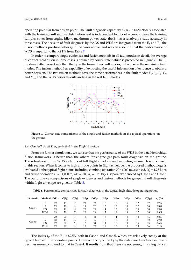
operating point far from design point. The fault diagnosis capability by RR-KELM closely associatedwith the training fault sample distribution and is independent to model accuracy. Since the trainingsamples cover from engine idle to maximum power state, the E2 has a relatively steady accuracy inthree cases. The decision of fault diagnosis by the DS and WDS are integrated from the E1 and E2, thefusion methods produce better rp in the cases above, and we can also find that the performance ofWDS is superior to that of DS from Table 7.

In order to compare single evidences and fusion methods in all fault modes in detail, the averageof correct recognition in three cases is defined by correct rate, which is presented in Figure 7. The E1produce better correct rate than the E2 in the former two fault modes, but worse in the remaining faultmodes. The fusion method has capability of extracting the useful information of evidence to obtain abetter decision. The two fusion methods have the same performances in the fault modes F1, F2, F3, F7,and F10, and the WDS performs outstanding in the rest fault modes.

Energies 2016, 9, 828 17 of 23

Table 7. Fault diagnostic performance comparisons of the involved methods in the typical operations

on the ground.

Scenario Method C(F1) C(F2) C(F3) C(F4) C(F5) C(F6) C(F7) C(F8) C(F9) C(F10) rp (%)

Case 1

E1 19 19 15 18 17 18 19 15 19 17 88.0

E2 17 17 16 20 18 19 20 15 20 15 88.5

DS 20 19 17 20 18 19 20 18 20 19 95.0

WDS 20 19 18 20 20 19 20 19 20 19 97.0

Case 2

E1 16 18 16 19 16 17 16 17 17 16 84.0

E2 13 17 18 18 18 18 17 17 16 18 85.0

DS 16 19 18 19 19 18 19 18 17 18 90.5

WDS 17 18 18 20 20 18 18 19 17 18 91.5

Case 3

E1 18 19 14 19 18 16 15 16 17 14 83.0

E2 19 16 19 18 18 15 17 16 19 15 86.0

DS 20 19 20 19 18 17 16 18 18 16 90.5

WDS 19 20 19 20 20 18 17 19 19 16 93.5

In order to compare single evidences and fusion methods in all fault modes in detail, the average

of correct recognition in three cases is defined by correct rate, which is presented in Figure 7. The E1

produce better correct rate than the E2 in the former two fault modes, but worse in the remaining

fault modes. The fusion method has capability of extracting the useful information of evidence to

obtain a better decision. The two fusion methods have the same performances in the fault modes F1,

F2, F3, F7, and F10, and the WDS performs outstanding in the rest fault modes.

Figure 7. Correct rate comparisons of the single and fusion methods in the typical operations on the ground.

4.4. Gas-Path Fault Diagnosis Test in the Flight Envelope

From the former simulations, we can see that the performance of the WDS in the data

hierarchical fusion framework is better than the others for engine gas-path fault diagnosis on the

ground. The robustness of the WDS in terms of full flight envelope and modeling mismatch is

discussed in this section. When it comes to high altitude points in flight envelope, the proposed

methodology is evaluated at the typical flight points including climbing operation H = 6000 m, Ma =

0.5, Wf = 1.28 kg/s and cruise operation H = 11,000 m, Ma = 0.8, Wf = 0.78 kg/s, separately denoted by

Case 4 and Case 5. The performance comparisons of single evidences and fusion methods for gas-

path fault diagnosis within flight envelope are given in Table 8.

Figure 7. Correct rate comparisons of the single and fusion methods in the typical operations onthe ground.

4.4. Gas-Path Fault Diagnosis Test in the Flight Envelope

From the former simulations, we can see that the performance of the WDS in the data hierarchicalfusion framework is better than the others for engine gas-path fault diagnosis on the ground.The robustness of the WDS in terms of full flight envelope and modeling mismatch is discussedin this section. When it comes to high altitude points in flight envelope, the proposed methodology isevaluated at the typical flight points including climbing operation H = 6000 m, Ma = 0.5, Wf = 1.28 kg/sand cruise operation H = 11,000 m, Ma = 0.8, Wf = 0.78 kg/s, separately denoted by Case 4 and Case 5.The performance comparisons of single evidences and fusion methods for gas-path fault diagnosiswithin flight envelope are given in Table 8.

Table 8. Performance comparisons for fault diagnosis in the typical high altitude operating points.

Scenario Method C(F1) C(F2) C(F3) C(F4) C(F5) C(F6) C(F7) C(F8) C(F9) C(F10) rp (%)

Case 4

E1 19 19 13 20 19 16 15 15 12 17 82.5E2 19 18 19 19 12 13 17 18 17 14 83.0DS 19 19 19 20 19 14 17 18 15 18 89.0

WDS 19 20 20 20 19 17 18 19 17 18 93.5

Case 5

E1 20 20 13 19 18 13 14 18 14 16 82.5E2 18 19 19 16 15 10 16 18 11 12 77.0DS 19 20 20 17 18 14 16 19 15 15 86.5

WDS 19 20 19 18 19 17 17 19 19 16 91.5

The index rp of the E1 is 82.5% both in Case 4 and Case 5, which are relatively steady at thetypical high altitude operating points. However, the rp of the E2 by the data-based evidence in Case 5declines more compared to that in Case 4. It results from that there are not enough training data at

Energies 2016, 9, 828 18 of 22

the high altitude operating points. The E1 decision brought from the model-based evidence is closelydependent on physical thermodynamics and component map of turbofan engine. It is hardly affectedby the training data as the E2, thus the E1 has a better robustness of fault diagnosis than the E2 in theflight envelope. The results calculated by the DS and WDS are closer to the true state than those bytwo evidences. The WDS’s rp is more than 90% in two cases above and it produces the best accuracyof fault diagnosis in Case 4 and Case 5. Ten trials are conducted for each fault scenario with everyapproach, and the averages of correct rate by the evidences and fusion methods in Case 4 and Case 5are shown in Figure 8. Compared to the E1, E2 and DS, the WDS has the best correct rate except in thefault modes F1 and F4 from Figure 8. Consequently, the data hierarchical fusion based on the WDS hasa satisfactory robustness at high altitude operating points in the flight envelope.

Energies 2016, 9, 828 18 of 23

Table 8. Performance comparisons for fault diagnosis in the typical high altitude operating points.

Scenario Method C(F1) C(F2) C(F3) C(F4) C(F5) C(F6) C(F7) C(F8) C(F9) C(F10) rp (%)

Case 4

E1 19 19 13 20 19 16 15 15 12 17 82.5

E2 19 18 19 19 12 13 17 18 17 14 83.0

DS 19 19 19 20 19 14 17 18 15 18 89.0

WDS 19 20 20 20 19 17 18 19 17 18 93.5

Case 5

E1 20 20 13 19 18 13 14 18 14 16 82.5

E2 18 19 19 16 15 10 16 18 11 12 77.0

DS 19 20 20 17 18 14 16 19 15 15 86.5

WDS 19 20 19 18 19 17 17 19 19 16 91.5

The index rp of the E1 is 82.5% both in Case 4 and Case 5, which are relatively steady at the typical

high altitude operating points. However, the rp of the E2 by the data-based evidence in Case 5 declines

more compared to that in Case 4. It results from that there are not enough training data at the high

altitude operating points. The E1 decision brought from the model-based evidence is closely

dependent on physical thermodynamics and component map of turbofan engine. It is hardly affected

by the training data as the E2, thus the E1 has a better robustness of fault diagnosis than the E2 in the

flight envelope. The results calculated by the DS and WDS are closer to the true state than those by

two evidences. The WDS’s rp is more than 90% in two cases above and it produces the best accuracy

of fault diagnosis in Case 4 and Case 5. Ten trials are conducted for each fault scenario with every

approach, and the averages of correct rate by the evidences and fusion methods in Case 4 and Case 5

are shown in Figure 8. Compared to the E1, E2 and DS, the WDS has the best correct rate except in the

fault modes F1 and F4 from Figure 8. Consequently, the data hierarchical fusion based on the WDS

has a satisfactory robustness at high altitude operating points in the flight envelope.

Figure 8. Correction rate average comparisons of evidence and fusion methods in the flight envelope.

4.5. Robust Test with Modeling Uncertainty

The tests completed above are assuming that the engine model tracks actual engine well, but the

modeling mismatch between the engine CLM and actual individual is inevitable in practice. The

engine manufacture tolerances lead to the individual performance difference under nominal

operating conditions, and the engine-to-engine variation is one of the most important reasons to

cause the modeling uncertainty. The modeling uncertainty of turbofan engine can be represented by

modeling errors, and it will affect the performance of model-based method. The robustness

evaluation of the proposed fusion framework with regards to modeling uncertainty is performed in

Case 1, Case 4 and Case 5. The modeling errors of key measurement shown in Table 2 are added to

the engine CLM outputs. Fault diagnostic performance comparisons of the evidences and fusion

methods with modeling uncertainty in flight envelope are given in Table 9.

Figure 8. Correction rate average comparisons of evidence and fusion methods in the flight envelope.

4.5. Robust Test with Modeling Uncertainty

The tests completed above are assuming that the engine model tracks actual engine well,but the modeling mismatch between the engine CLM and actual individual is inevitable in practice.The engine manufacture tolerances lead to the individual performance difference under nominaloperating conditions, and the engine-to-engine variation is one of the most important reasons tocause the modeling uncertainty. The modeling uncertainty of turbofan engine can be represented bymodeling errors, and it will affect the performance of model-based method. The robustness evaluationof the proposed fusion framework with regards to modeling uncertainty is performed in Case 1,Case 4 and Case 5. The modeling errors of key measurement shown in Table 2 are added to the engineCLM outputs. Fault diagnostic performance comparisons of the evidences and fusion methods withmodeling uncertainty in flight envelope are given in Table 9.

The indices rp of the E1 in three cases are less than 80% when the modeling mismatch is considered,and those indices of fusion methods are also declined since one evidence accuracy decrease. While therp of WDS both in Case 1 and Case 4 are still more than 90%, and the correct recognition number bythe WDS is more than that by the DS. It indicates that the WDS has better accuracy of fault diagnosticsthan the DS in the cases of modeling uncertainty. In order to further present the robustness of datahierarchical fusion scheme, the correct rate average of 10 trials of three cases (Case 1, Case 4 andCase 5) in 10 fault modes are shown in Figure 9. As can be seen from Figure 9, the correct rate averageof fusion methods declines as the modeling errors is injected. The DS produces more reduction ofcorrect rate than the WDS except in three fault modes F6, F7, and F9. Besides, the maximum decline bythe WDS is 0.05 while that by the DS is near 0.12. That is to say, the fluctuation by the WDS is less thanthat by the DS when the modeling uncertainty is considered. In a word, despite the CLM modelingmismatch of turbofan engine, the robustness of data hierarchical fusion framework based on WDS is abetter candidate for gas-path fault diagnosis.

Energies 2016, 9, 828 19 of 22

Table 9. Fault diagnostic performance comparisons of the involved methods with modeling uncertainty.

Scenario Method C(F1) C(F2) C(F3) C(F4) C(F5) C(F6) C(F7) C(F8) C(F9) C(F10) rp (%)

Case 1

E1 17 10 12 15 19 18 15 17 13 19 77.5E2 17 17 16 20 18 19 20 15 20 15 88.5DS 16 19 17 19 18 18 20 17 19 19 91.0

WDS 18 20 18 20 19 19 20 18 18 19 94.5

Case 4

E1 14 8 7 10 16 17 11 17 10 18 64.0E2 19 18 19 19 12 13 17 18 17 14 83.0DS 19 16 17 17 18 15 17 18 18 17 86.0

WDS 19 18 18 19 19 18 17 19 17 18 91.0

Case 5

E1 11 8 10 9 14 16 11 19 16 19 66.5E2 18 19 19 16 15 10 16 18 11 12 77.0DS 18 18 19 14 16 14 16 19 16 15 82.5

WDS 19 19 19 16 18 15 16 20 18 15 88.0

Energies 2016, 9, 828 19 of 23

Table 9. Fault diagnostic performance comparisons of the involved methods with modeling uncertainty.

Scenario Method C(F1) C(F2) C(F3) C(F4) C(F5) C(F6) C(F7) C(F8) C(F9) C(F10) rp (%)

Case 1

E1 17 10 12 15 19 18 15 17 13 19 77.5

E2 17 17 16 20 18 19 20 15 20 15 88.5

DS 16 19 17 19 18 18 20 17 19 19 91.0

WDS 18 20 18 20 19 19 20 18 18 19 94.5

Case 4

E1 14 8 7 10 16 17 11 17 10 18 64.0

E2 19 18 19 19 12 13 17 18 17 14 83.0

DS 19 16 17 17 18 15 17 18 18 17 86.0

WDS 19 18 18 19 19 18 17 19 17 18 91.0

Case 5

E1 11 8 10 9 14 16 11 19 16 19 66.5

E2 18 19 19 16 15 10 16 18 11 12 77.0

DS 18 18 19 14 16 14 16 19 16 15 82.5

WDS 19 19 19 16 18 15 16 20 18 15 88.0

The indices rp of the E1 in three cases are less than 80% when the modeling mismatch is

considered, and those indices of fusion methods are also declined since one evidence accuracy

decrease. While the rp of WDS both in Case 1 and Case 4 are still more than 90%, and the correct

recognition number by the WDS is more than that by the DS. It indicates that the WDS has better

accuracy of fault diagnostics than the DS in the cases of modeling uncertainty. In order to further

present the robustness of data hierarchical fusion scheme, the correct rate average of 10 trials of three

cases (Case 1, Case 4 and Case 5) in 10 fault modes are shown in Figure 9. As can be seen from Figure

9, the correct rate average of fusion methods declines as the modeling errors is injected. The DS

produces more reduction of correct rate than the WDS except in three fault modes F6, F7, and F9.

Besides, the maximum decline by the WDS is 0.05 while that by the DS is near 0.12. That is to say, the

fluctuation by the WDS is less than that by the DS when the modeling uncertainty is considered. In a

word, despite the CLM modeling mismatch of turbofan engine, the robustness of data hierarchical

fusion framework based on WDS is a better candidate for gas-path fault diagnosis.

Figure 9. Correct rate average declines of fusion methods with modeling uncertainty in flight envelope.

5. Conclusions

This paper develops a systematic approach including data processing and fusion mechanism

which lead to an improved data hierarchical fusion framework. The novelty of this methodology lies

in the development of a data fusion technique that combines sub-decisions from two different ways

of fault diagnosis, namely, the model-based and data-driven methods. By computing and combining

the fault mode index and fault probability of the evidences, a fused faulty index is designed to better

identify gas-path failure mode for turbofan engine. Guidelines for several key elements related to the

problem formulation, fault feature description, fusion scheme, fault diagnostic robustness and other

important aspects are discussed and illustrated in the case study. The proposed RR-KELM algorithm

brings sparseness of training data and simplifies topological structure of the learning machine, which

is used to generate data-based evidence. One advantage of this methodology is that the fault pattern

recognition becomes more accurate than the single evidence (the model-based or data-based one).

Figure 9. Correct rate average declines of fusion methods with modeling uncertainty in flight envelope.

5. Conclusions

This paper develops a systematic approach including data processing and fusion mechanismwhich lead to an improved data hierarchical fusion framework. The novelty of this methodology liesin the development of a data fusion technique that combines sub-decisions from two different ways offault diagnosis, namely, the model-based and data-driven methods. By computing and combiningthe fault mode index and fault probability of the evidences, a fused faulty index is designed to betteridentify gas-path failure mode for turbofan engine. Guidelines for several key elements related to theproblem formulation, fault feature description, fusion scheme, fault diagnostic robustness and otherimportant aspects are discussed and illustrated in the case study. The proposed RR-KELM algorithmbrings sparseness of training data and simplifies topological structure of the learning machine, whichis used to generate data-based evidence. One advantage of this methodology is that the fault patternrecognition becomes more accurate than the single evidence (the model-based or data-based one). Thisproperty could have a great impact on deciding whether to stop operation and to schedule maintenancefor turbofan engine. Another advantage of this methodology is that the robustness of fault diagnosissignificantly improved in terms of various operations in flight envelope and modeling uncertainty,and it implies that the data hierarchical fusion can be a more efficient tool in practice.

The methodology is validated using the faulty operating data of turbofan engine that are generatedby the general gas turbine simulation. The model-based method using the PF-FL algorithm and thedata-based method using the RR-KELM algorithm are served to produce fault diagnostic evidencesin feature layer. It is proved that the RR-KELM is well trade-off between the classification accuracyand topology simplification. The fault mode index and fault probability related to each evidence areintegrated by the fusion scheme to reach a final decision of gas-path fault diagnosis in decision layer.In the data hierarchical fusion architecture, the WDS is developed from the DS for integrating multipleevidence information with evidence reliability coefficients. The stochastic fault operating data areadopted to numerically evaluate the capability of the proposed methodology, and the performance

Energies 2016, 9, 828 20 of 22

comparisons of single and fusion methods are completed in the typical operations. In addition, thetests about modeling mismatch and lack of training data covering all fault modes are discussed inthe flight envelope. Since the proposed methodology integrates the advantage of model-based anddata-based methods, the confidence and robustness for gas-path fault diagnosis is expected to beimproved by drawing more useful information of evidences.

This research establishes a new direction at information fusion by proposing a data hierarchicalfusion technique that is specifically beneficial for engine gas-path fault diagnosis applications.There are several important topics for future research that are related to this work. First, furtherstudies can be done to investigate the performance when engine gas-path fault feature selection andthe kernel methods are used to fault feature extraction. Except for the efficiency of engine component,flow capacity could be added into fault feature parameters. Second, although this paper focuses onthe engine gas-path fault diagnosis at one cycle number and no degradation considered, extensionsto the cases of normal engine performance degeneration in the course of its lifetime are worthy offurther exploration.

Acknowledgments: We are grateful for the financial support of the National Nature Science Foundation of China(No. 61304133), and China Outstanding Postdoctoral Science Foundation (No.2015T80552). Gratitude is alsoextended to Viliam Makis for useful suggestions and to China Scholarship Council for supporting the first authorto carry out collaborative research in the Department of Mechanical and Industrial Engineering at the Universityof Toronto.

Author Contributions: Feng Lu and Jinquan Huang contributed in developing the ideas of this research.Yafan Wang, Chengxin You and Chunyu Jiang performed this research. All of the authors were involvedin preparing this manuscript.

Conflicts of Interest: The authors declare no conflict of interest.

Abbreviations

The following abbreviations are used in this manuscript:

GPA Gas-path analysisNN Neural networkELM Extreme learning machineKF Kalman filterPF Particle filterFL Fuzzy logicDS Dempster–Shaffer evidence theoryHPT High pressure turbineLPT Low pressure turbinex State vectory Measured vectorh Health parameterw Process noise Vectorv Measurement noise vectorQ Covariance of process noiseR Covariance of measurement noiseNL Low pressure rotor speedNH High pressure rotor speedSE1 Variation of fan efficiencySE2 Variation of compressor efficiencySE3 Variation of HPT efficiencySE4 Variation of LPT efficiencyWf Fuel flow rateA8 Nozzle areaT22 Fan outlet temperatureP22 Fan outlet pressureT3 Compressor outlet temperatureP3 Compressor outlet pressureT43 LPT inlet temperatureT6 LPT outlet temperaturerp Correct percentage

Energies 2016, 9, 828 21 of 22

References

1. Volponi, A.J. Gas turbine engine health management: Past, present, and future trends. ASME J. Eng. GasTurbines Power 2014, 136, 051201. [CrossRef]

2. Zaidan, M.A.; Mills, A.R.; Harrison, R.F.; Fleming, P.J. Gas turbine engine prognostics using Bayesianhierarchical models: A variational approach. Mech. Syst. Signal Process. 2016, 70–71, 120–140. [CrossRef]

3. Lamaris, V.T.; Hountalas, D.T. A general purpose diagnostic technique for marine dieselengines—Application on the main propulsion and auxiliary diesel units of a marine vessel. Energy Convers.Manag. 2010, 51, 740–753. [CrossRef]

4. Kraft, J.; Sethi, V.; Singh, R. Optimization of aero gas turbine maintenance using advanced simulation anddiagnostic methods. ASME J. Eng. Gas Turbines Power 2014, 136, 111601. [CrossRef]

5. Zhang, X.D.; Tang, L.; Decastro, J.A. Robust fault diagnosis of aircraft engines: A nonlinear adaptiveestimation-based approach. IEEE Trans. Control Syst. Technol. 2013, 21, 861–868.

6. Li, Y.G.; Korakianitis, T. Nonlinear weighted-least-squares estimation approach for gas-turbine diagnosticapplications. J. Propuls. Power 2011, 27, 337–345. [CrossRef]

7. Simon, D.L.; Armstrong, J.B. An integrated approach for aircraft engine performance estimation and faultdiagnostics. ASME J. Eng. Gas Turbines Power 2013, 135, 071203. [CrossRef]

8. Pourbabaee, B.; Meskin, N.; Khorasani, K. Sensor fault detection, isolation, and identification usingmultiple-model-based hybrid Kalman filter for gas turbine engines. IEEE Trans. Control Syst. Technol.2015, 24. [CrossRef]

9. Lu, F.; Huang, J.Q.; Lv, Y.Q. Gas path health monitoring for a turbofan engine based on a nonlinear filteringapproach. Energies 2013, 6, 492–513. [CrossRef]

10. Simon, D. A comparison of filtering approaches for aircraft engine health estimation. Aerosp. Sci. Technol.2008, 12, 276–284. [CrossRef]

11. Borguet, S.; Léonard, O. Comparison of adaptive filters for gas turbine performance monitoring. J. Comput.Appl. Math. 2010, 234, 2202–2212. [CrossRef]

12. Barelli, L.; Bidini, G.; Bonucci, F. Diagnosis of a turbocharging system of 1 MW internal combustion engine.Energy Convers. Manag. 2013, 68, 23–39. [CrossRef]

13. Bettocchi, R.; Pinelli, M.; Spina, P.R.; Venturini, M. Artificial intelligence for the diagnostics of gasturbines-part 2: Neuro-fuzzy approach. ASME J. Eng. Gas Turbines Power 2006, 129, 720–729. [CrossRef]

14. Sampath, S.; Singh, R. An integrated fault diagnostics model using genetic algorithm and neural networks.ASME J. Eng. Gas Turbines Power 2006, 128, 49–56. [CrossRef]

15. Tayarani-Bathaie, S.S.; Khorasani, K. Fault detection and isolation of gas turbine engines using a bank ofneural networks. J. Process Control 2015, 36, 22–41. [CrossRef]

16. Mohammadi, E.; Montazeri-Gh, M. Performance enhancement of global optimization-based gas turbinefault diagnosis systems. J. Propuls. Power 2016, 32, 214–224. [CrossRef]

17. Urban, L.A. Gas Turbine Engine Parameter Interrelationships, 2nd ed.; Hamilton Standard Division of UnitedAircraft Corp. (HSDUTC): Windsor Locks, CT, USA, 1969.

18. Lu, F.; Wang, Y.F.; Huang, J.Q.; Huang, Y.H. Gas turbine transient performance tracking using data fusionbased on an adaptive particle filter. Energies 2015, 8, 13911–13927. [CrossRef]

19. Hanachi, H.; Liu, J.; Banerjee, A.; Chen, Y. Sequential state estimation of nonlinear/non-Gaussian systemswith stochastic input for turbine degradation estimation. Mech. Syst. Signal Process. 2016, 72–73, 32–45.[CrossRef]

20. Decastro, J.A.; Frederick, D.K.; Tang, L. Engine Parameter Estimation in Test Cells Using Hybrid Physics/EmpiricalModels; ASME Paper No. GT2011-45633; ASME: New York, NY, USA, 2011.

21. Pourbabaee, B.; Meskin, N.; Khorasani, K. Robust sensor fault detection and isolation of gas turbineengines subjected to time-varying parameter uncertainties. Mech. Syst. Signal Process. 2016, 76–77, 136–156.[CrossRef]

22. Amozegar, M.; Khorasani, K. An ensemble of dynamic neural network identifiers for fault detection andisolation of gas turbine engines. Neural Netw. 2016, 76, 106–121. [CrossRef] [PubMed]

23. Barad, S.G.; Ramaiah, P.V.; Giridhar, R.K.; Krishnaiah, G. Neural network approach for a combinedperformance and mechanical health monitoring of a gas turbine engine. Mech. Syst. Signal Process. 2012, 27,729–742. [CrossRef]

Energies 2016, 9, 828 22 of 22

24. Cortes, C.; Vapnik, V. Support-vector network. Mach. Learn. 1995, 20, 273–297. [CrossRef]25. Fei, S.W. A hybrid model of EMD and multiple-kernel RVR algorithm for wind speed prediction. Int. J.

Electr. Power Energy Syst. 2016, 78, 910–915. [CrossRef]26. Zhou, D.J.; Zhang, H.S.; Weng, S.L. A new gas path fault diagnostic method of gas turbine based on support

vector machine. ASME J. Eng. Gas Turbines Power 2015, 137, 102605. [CrossRef]27. Huang, G.B.; Zhou, H.M.; Ding, X.J.; Zhang, R. Extreme learning machine for regression and multiclass

classification. IEEE Trans. Syst. Man Cybern. 2012, 42, 513–529. [CrossRef] [PubMed]28. Yang, Y.M.; Wang, Y.N.; Yuan, X.F. Bidirectional extreme learning machine for regression problem and its

learning effectiveness. IEEE Trans. Neural Netw. Learn/Syst. 2012, 23, 1498–1505. [CrossRef] [PubMed]29. Luo, J.; Vong, C.M.; Wong, P.K. Sparse Bayesian extreme learning machine for multi-classification.

IEEE Trans. Neural Netw. Learn. Syst. 2014, 25, 836–843. [PubMed]30. Bai, Z.; Huang, G.B.; Wang, D.W.; Wang, H.; Westover, M.B. Sparse extreme learning machine for

classification. IEEE Trans. Cybern. 2014, 44, 1858–1870. [CrossRef] [PubMed]31. Li, X.; Mao, W.; Jiang, W. Fast sparse approximation of extreme learning machine. Neurocomputing 2014, 128,

96–103. [CrossRef]32. Liu, K.; Gebraeel, N.Z.; Shi, J. A data-level fusion model for developing composite health indices for

degradation modeling and prognostic analysis. IEEE Trans. Autom. Sci. Eng. 2013, 10, 652–664. [CrossRef]33. Kyriazis, A.; Mathioudakis, K. Gas turbine fault diagnosis using fuzzy-based decision fusion. J. Propuls.

Power 2009, 25, 335–343. [CrossRef]34. Butler, S.W.; Pattipati, K.R.; Volponi, A.; Hull, J.; Rajamani, R.; Siegel, J. An Assessment Methodology for

Data-Driven and Model-Based Techniques for Engine Health Monitoring; American Society of MechanicalEngineers (ASME): New York, NY, USA, 2006.

35. Chacartegui, R.; Sanchez, D.; Munoz, A.; Sanchez, T. Real Time Simulation of Medium Size Gas Turbines.Energy Convers. Manag. 2011, 52, 713–724. [CrossRef]

36. Sun, J.G.; Vasilyev, V.; Ilyasov, B. Advanced Multivariable Control Systems of Aeroengines; Beihang Press: Beijing,China, 2005; pp. 60–108.

37. Chen, H.L.; Wang, G.; Ma, C.; Cai, Z.N.; Liu, W.B.; Wang, S.J. An efficient hybrid kernel extreme learningmachine approach for early diagnosis of Parkinson’s disease. Neurocomputing 2016, 184, 131–144. [CrossRef]

38. Subrahmanya, N.; Shin, Y.C.; Meckl, P.H. A Bayesian machine learning method for sensor selection andfusion with application to on-board fault diagnostics. Mech. Syst. Signal Process. 2010, 24, 182–192. [CrossRef]

39. Basir, O.; Yuan, X. Engine fault diagnosis based on multi-sensor information fusion using dempster-shaferevidence theory. Inform. Fusion 2007, 8, 379–386. [CrossRef]

40. Zhou, W.X. Research on Object-Oriented Modeling and Simulation for Aeroengine and Control System.Ph.D. Thesis, Nanjing University of Aeronautics and Astronautics, Nanjing, Jiangsu, China, 2007.

41. Gordon, N.; Salmond, D.; Smith, A. Novel approach to nonlinear/non-Gaussian bayesian state estimation.IEE Proc. F Radar Signal Process 1993, 140, 107–113. [CrossRef]

42. Aditya, K.; Daniel, V. Model-Based Fault Tolerant Control; National Aeronautics and Space Administration(NASA): Greenbelt, MD, USA, 2008.

43. Jousselme, A.L.; Maupin, P. Distances in Evidence theory: Comprehensive survey and generalizations. Int. J.Approx. Reason. 2012, 53, 118–145. [CrossRef]

44. Deng, X.; Liu, Q.; Deng, Y.; Mahadevan, S. An improved method to construct basic probability assignmentbased on the confusion matrix for classification problem. Inform. Sci. 2016, 340, 250–261. [CrossRef]

45. Lu, F.; Zheng, W.H.; Huang, J.Q.; Feng, M. Life cycle performance estimation and in-flight health monitoringfor gas turbine engine. ASME J. Dyn. Syst. Meas. Control 2016, 138, 091009. [CrossRef]

© 2016 by the authors; licensee MDPI, Basel, Switzerland. This article is an open accessarticle distributed under the terms and conditions of the Creative Commons Attribution(CC-BY) license (http://creativecommons.org/licenses/by/4.0/).