NeuroImage 101 (2014) 569–582

Contents lists available at ScienceDirect

NeuroImage

j ourna l homepage: www.e lsev ie r .com/ locate /yn img

Hierarchical feature representation and multimodal fusion with deeplearning for AD/MCI diagnosis

Heung-Il Suk a, Seong-Whan Lee b, Dinggang Shen a,b,⁎, the Alzheimer's Disease Neuroimaging Initiative 1

a Department of Radiology and Biomedical Research Imaging Center (BRIC), University of North Carolina at Chapel Hill, NC, USAb Department of Brain and Cognitive Engineering, Korea University, Seoul, Republic of Korea

⁎ Corresponding author at: Department of Radiology anCenter (BRIC), University of North Carolina at Chapel Hill,

E-mail address: dgshen@med.unc.edu (D. Shen).1 Data used in preparation of this article were obtaine

Neuroimaging Initiative (ADNI) database (http://www.loinvestigators within the ADNI contributed to the designand/or provided data but did not participate in analysis or wlist of ADNI investigators is available at http://adni.loni.uclto_apply/ADNI_Authorship_List.pdf.

2 Although it is clear from the context that the acronymMachine” in this paper, we would clearly indicate tha“Deformation Based Morphometry”.

http://dx.doi.org/10.1016/j.neuroimage.2014.06.0771053-8119/© 2014 Elsevier Inc. All rights reserved.

a b s t r a c t

a r t i c l e i n f o

Article history:Accepted 28 June 2014Available online 18 July 2014

Keywords:Alzheimer's DiseaseMild Cognitive ImpairmentMultimodal data fusionDeep Boltzmann MachineShared feature representation

For the last decade, it has been shown that neuroimaging can be a potential tool for the diagnosis of Alzheimer'sDisease (AD) and its prodromal stage, Mild Cognitive Impairment (MCI), and also fusion of different modalities canfurther provide the complementary information to enhance diagnostic accuracy. Here, we focus on the problems ofboth feature representation and fusion of multimodal information from Magnetic Resonance Imaging (MRI) andPositron Emission Tomography (PET). To our best knowledge, the previous methods in the literature mostly usedhand-crafted features such as cortical thickness, gray matter densities from MRI, or voxel intensities from PET,and then combined these multimodal features by simply concatenating into a long vector or transforming into ahigher-dimensional kernel space. In this paper, we propose a novel method for a high-level latent and sharedfeature representation from neuroimaging modalities via deep learning. Specifically, we use Deep BoltzmannMachine (DBM)2, a deep network with a restricted Boltzmann machine as a building block, to find a latent hierar-chical feature representation from a 3D patch, and then devise a systematic method for a joint feature representa-tion from the paired patches of MRI and PET with a multimodal DBM. To validate the effectiveness of the proposedmethod, we performed experiments on ADNI dataset and compared with the state-of-the-art methods. In threebinary classification problems of AD vs. healthy Normal Control (NC), MCI vs. NC, and MCI converter vs. MCInon-converter, we obtained the maximal accuracies of 95.35%, 85.67%, and 74.58%, respectively, outperformingthe competing methods. By visual inspection of the trained model, we observed that the proposed method couldhierarchically discover the complex latent patterns inherent in both MRI and PET.

d Biomedical Research ImagingNC, USA.

d from the Alzheimer's Diseaseni.ucla.edu/ADNI). As such, theand implementation of ADNIriting of this report. A completea.edu/wpcontent/uploads/how_

DBMdenotes “Deep Boltzmannt DBM here is not related to

© 2014 Elsevier Inc. All rights reserved.

Introduction

Alzheimer's Disease (AD), characterized by progressive impairmentof cognitive and memory functions, is the most prevalent cause of de-mentia in elderly subjects. According to a recent report by Alzheimer'sAssociation, the number of subjects with AD is significantly increasingevery year, and 10 to 20% of people aged 65 or older haveMild CognitiveImpairment (MCI), known as a prodromal stage of AD (Alzheimer'sAssociation, 2012). However, due to the limited period for which thesymptomatic treatments could be effective, it has been of great impor-tance for early diagnosis and prognosis of AD/MCI in the clinic.

To this end, many researchers have devoted their efforts to findbiomarkers and develop a computer-aided system, with which we caneffectively predict or diagnose the diseases. Recent studies haveshown that the neuroimaging such as Magnetic Resonance Imaging(MRI) (Cuingnet et al., 2011; Davatzikos et al., 2011; Li et al., 2012;Wee et al., 2011; Zhang et al., 2012; Zhou et al., 2011), Positron EmissionTomography (PET) (Nordberg et al., 2010), and functional MRI (fMRI)(Greicius et al., 2004; Suk et al., 2013), can be nice tools for diagnosisor prognosis of AD/MCI. Furthermore, fusing the complementary infor-mation frommultiple modalities helps enhance the diagnostic accuracy(Cui et al., 2011; Fan et al., 2007a; Hinrichs et al., 2011; Kohannim et al.,2010; Perrin et al., 2009; Suk and Shen, 2013;Walhovd et al., 2010;Weeet al., 2012; Westman et al., 2012; Yuan et al., 2012; Zhang and Shen,2012; Zhang et al., 2011).

Various types of features or patterns extracted from neuroimagingmodalities have been considered for brain disease diagnosis withmachine learningmethods. Here, we divide the previous feature extrac-tion approaches into three categories: voxel-based approach, Region OfInterest (ROI)-based approach, and patch-based approach. A voxel-based approach is themost simple and directway that uses the voxel in-tensities as features in classification (Baron et al., 2001; Ishii et al.,2005). Although it is simple and intuitive in terms of interpretation of

3 Available at ‘http://www.loni.ucla.edu/ADNI’.4 Although there exist in total more than 800 subjects in ADNI database, only 398 sub-

jects have the baseline data including the modalities of both MRI and FDG-PET.5 Refer to ‘http://www.adniinfo.org’ for the details.

570 H.-I. Suk et al. / NeuroImage 101 (2014) 569–582

the results, its main limitations are the high-dimensionality of featurevectors and also the ignorance of regional information. ROI-basedapproach considers the structurally or functionally predefined brain re-gions and extracts representative features from each region (Cuingnetet al., 2011; Davatzikos et al., 2011; Kohannim et al., 2010; Nordberget al., 2010; Suk and Shen, 2013; Walhovd et al., 2010; Zhang andShen, 2012). Thanks to the relatively low feature dimensionality andthe whole brain coverage, it is widely used in the literature. However,the features extracted from ROIs are very coarse in the sense that theycannot reflect small or subtle changes involved in the brain diseases.Note that the disease-related structural/functional changes occur inmultiple brain regions. Furthermore, since the abnormal regions affectedby neurodegenerative diseases can be part of ROIs or span over multipleROIs, the simple voxel- or ROI-based approach may not effectivelycapture the diseased-related pathologies. To tackle these limitations, re-cently, Liu et al. proposed a patch-basedmethod that first dissected brainareas into small 3D patches, extracted features from each selected patchindividually, and then combined the features hierarchically in a classifierlevel (Liu et al., 2012, 2013).

As for the fusion ofmultiplemodalities includingMRI, PET, biologicaland neurological data for discriminating AD/MCI patients from healthyNormal Control (NC), Kohannim et al. (2010) concatenated featuresfrom modalities into a vector and used a Support Vector Machine(SVM) classifier. Walhovd et al. (2010) applied multi-method stepwiselogistic regression analyses, and Westman et al. (2012) exploited ahierarchical modeling of orthogonal partial least squares to latentstructures. Hinrichs et al. (2011), Suk and Shen (2013), and Zhanget al. (2011), independently, utilized a kernel-based machine learningtechnique.

In this paper, we consider the problems of both feature representa-tion and multimodal data fusion for computer-aided AD/MCI diagnosis.Specifically, for feature representation, we exploit a patch-basedapproach since it can be considered as an intermediate level betweenvoxel-based approach and ROI-based approach, thus efficiently han-dling the concerns of the high feature dimension and also the sensitivityto small change. Furthermore, from a clinical perspective, neurologistsor radiologists examine brain images by searching local distinctive re-gions and then combine the interpretations with neighboring onesand ultimately with the whole brain. In these regards, we believe thatthe patch-based approach can effectively handle the region-widepathologies, which may not be limited to specific ROIs, and accordswith the neurologists or radiologists' perspective in terms of examiningimages, i.e., investigating local patterns and then combining local infor-mation distributed in the whole brain for making a clinical decision. Inthis way, we can also extract richer information that helps enhancediagnostic accuracy.

However, unlike Liu et al.'s method that directly used the graymatterdensity values in each patch as features, we propose to use a latent high-level feature representation. Meanwhile, in the fusion of multimodalinformation, the previous methods often applied either simple concate-nation of features extracted frommultiple modalities or kernel methodsto combine them in a high-dimensional kernel space. However, thefeature extraction and feature combination were often performed inde-pendently. In this work, we propose a novel method of extracting ashared feature representation from multiple modalities, i.e., MRI andPET. As investigated in the previous studies (Catana et al., 2012; Pichleret al., 2010), there exist the inherent relations between modalities ofMRI and PET. Thus, finding the shared feature representation, whichcombines the complementary information from modalities, is helpfulto enhance performance on AD/MCI diagnosis.

From a feature representation perspective, it is noteworthy thatunlike the previous approaches (Hinrichs et al., 2011; Kohannim et al.,2010; Liu et al., 2012, 2013; Walhovd et al., 2010; Westman et al.,2012; Zhang and Shen, 2012; Zhang et al., 2011) that considered simplelow-level features, which are often vulnerable to noises, we propose toconsider high-level or abstract features for improving the robustness to

noises. For obtaining the latent high-level feature representations in-herent in a patch observation such as correlations among voxels thatcover different brain regions, we exploit a deep learning strategy(Bengio, 2009; LeCun et al., 1998), which has been successfully ap-plied to medical imaging analysis (Ciresan et al., 2013; Hjelm et al.,2014; Liao et al., 2013; Shin et al., 2013; Suk and Shen, 2013).Among various deep models, we use a Deep Boltzmann Machine(DBM) (Salakhutdinov and Hinton, 2009) that can hierarchicallyfind feature representations in a probabilistic manner. Rather thanusing the noisy voxel intensities as features as Liu et al. (2013) did,the high-level representation obtained via DBM ismore robust to noisesand thus helps enhance diagnostic performances. Meanwhile, from amultimodal data fusion perspective, unlike the conventional multimod-al feature combination methods that first extract modality-specific fea-tures and then fuse their complementary information during classifierlearning, the proposed multimodal DBM fuses the complementary in-formation from different modalities during a feature representationstep. Note that oncewe extract features from eachmodality, wemay al-ready lose some good correlation information between modalities.Therefore, it is important to discover a shared representation by fullyutilizing the original information in eachmodality during feature repre-sentation procedure. In our multimodal data fusion method, thanks tothemethodological characteristic of the DBM (i.e., undirected graphicalmodel), it allows the bidirectional information flow from one modality(e.g.,MRI) to the othermodality (e.g., PET) and vice versa. Therefore,wecan distribute feature representations over different layers in the pathbetween modalities and thus efficiently discover a shared representa-tion while still utilizing the full information in the observations.

Materials and image processing

Subjects

In this work, we use the ADNI dataset publicly available on theweb,3 but consider only the baseline MRI and 18-Fluoro-DeoxyGlucosePET (FDG-PET) data acquired from 93 AD subjects, 204 MCI subjectsincluding 76 MCI converters (MCI-C) and 128 MCI non-converters(MCI-NC), and 101 NC subjects.4 The demographics of the subjects aredetailed in Table 1.

With regard to the general eligibility criteria in ADNI, subjects were inthe age of between 55 and 90with a study partner, who could provide anindependent evaluation of functioning. General inclusion/exclusioncriteria5 are as follows: 1) NC subjects: MMSE scores between 24 and30 (inclusive), a Clinical Dementia Rating (CDR) of 0, non-depressed,non-MCI, and non-demented; 2) MCI subjects: MMSE scores between24 and 30 (inclusive), a memory complaint, objective memory loss mea-sured by education adjusted scores on Wechsler Memory Scale LogicalMemory II, a CDR of 0.5, absence of significant levels of impairment inother cognitive domains, essentially preserved activities of daily living,and an absence of dementia; and 3) mild AD: MMSE scores between 20and 26 (inclusive), CDR of 0.5 or 1.0, and meets the National Institute ofNeurological and Communicative Disorders and Stroke and theAlzheimer's Disease and Related Disorders Association (NINCDS/ADRDA) criteria for probable AD.

MRI/PET scanning and image processing

The structural MR images were acquired from 1.5 T scanners. Wedownloaded data in the Neuroimaging Informatics Technology Initia-tive (NIfTI) format, which had been pre-processed for spatial distortioncorrection caused by gradient nonlinearity and B1 field inhomogeneity.

Table 1Demographic and clinical information of the subjects. (SD: standard deviation).

AD (93) MCI (204) NC (101)

Female/male 36/57 68/136 39/62Age (mean ± SD) [min–max] 75.49 ± 7.4 [55–88] 74.97 ± 7.2 [55–89] 75.93 ± 4.8 [62–87]Education (mean ± SD) [min–max] 14.66 ± 3.2 [4–20] 15.75 ± 2.9 [7–20] 15.83 ± 3.2 [7–20]MMSE (mean ± SD) [min–max] 23.45 ± 2.1 [18–27] 27.18 ± 1.7 [24–30] 28.93 ± 1.1 [25–30]CDR (mean ± SD) [min–max] 0.8 ± 0.25 [0.5–1] 0.5 ± 0.03 [0–0.5] 0 ± 0 [0–0]

571H.-I. Suk et al. / NeuroImage 101 (2014) 569–582

The FDG-PET images were acquired 30–60 min post-injection, averaged,spatially aligned, interpolated to a standard voxel size, normalized inintensity, and smoothed to a common resolution of 8 mm full width athalf maximum.

TheMR imageswere preprocessed by applying the typical proceduresof Anterior Commissure (AC)–Posterior Commissure (PC) correction,skull-stripping, and cerebellum removal. Specifically, we used MIPAVsoftware6 for AC–PC correction, resampled images to 256 × 256 × 256,and appliedN3 algorithm (Sled et al., 1998) to correct non-uniform tissueintensities. After skull stripping (Wang et al., 2014) and cerebellum re-moval, we manually checked the skull-stripped images to ensure theclean and dura removal. Then, FAST in FSL package7 (Zhang et al., 2001)was used to segment the structural MR images into three tissue types ofGray Matter (GM), White Matter (WM), and CerebroSpinal Fluid (CSF).Finally, all the three tissues of MR image were spatially normalizedonto a standard space, for which in this work we used a brain atlasalready aligned with the MNI coordinate space (Kabani et al., 1998),via HAMMER (Shen and Davatzikos, 2002), although other advancedregistration methods can also be applied for this process (Friston,1995; Jia et al., 2010; Tang et al., 2009; Xue et al., 2006; Yang et al.,2008). Then, the regional volumetric maps, called RAVENS maps, weregenerated by a tissue preserving image warping method (Davatzikoset al., 2001). It is noteworthy that the values of RAVENS maps are pro-portional to the amount of original tissue volume for each region, givinga quantitative representation of the spatial distribution of tissue types.Due to its relatively high relatedness to AD/MCI compared to WM andCSF (Liu et al., 2012), in this work, we considered only the spatiallynormalized GM volumes, called GM tissue densities, for classification.Regarding FDG-PET images, they were rigidly aligned to the respectiveMR images. The GM density maps and the PET images were furthersmoothed using a Gaussian kernel (with unit standard deviation) to im-prove the signal-to-noise ratio. We downsampled both the GM densitymaps and PET images to 64 × 64 × 64 voxels8 according to Liu et al.'s(2013) work, which saved the computational time and memory cost,but without sacrificing the classification accuracy.

Method

In Fig. 1, we illustrate a schematic diagram of our framework forAD/MCI diagnosis. Given a pair of MRI and PET images, we first selectclass-discriminative patches by means of a statistical significance testbetween classes. Using the tissue densities of a MRI patch and thevoxel intensities of a PET patch as observations, we build a patch-levelfeature learning model, called a MultiModal DBM (MM-DBM), thatfinds a shared feature representation from the paired patches. Here, in-stead of using the original real-valued tissue densities of MRI and thevoxel intensities of PET as inputs to MM-DBM, we first train a GaussianRestricted Boltzmann Machine (RBM) and use it as a preprocessor totransform the real-valued observations into binary vectors, which be-come the input to MM-DBM. After finding latent and shared featurerepresentations of the paired patches from the trained MM-DBM, weconstruct an image-level classifier by fusing multiple classifiers in a

6 Available at ‘http://mipav.cit.nih.gov/clickwrap.php’.7 Available at ‘http://fsl.fmrib.ox.ac.uk/fsl/fslwiki/’.8 The final voxel size is 4 × 4 × 4 mm3.

hierarchical manner, i.e., patch-level classifier learning, mega-patchconstruction, and a final ensemble classification.

Patch extraction

For the class-discriminative patch extraction, we exploit statisticalsignificance for voxels in each patch, i.e., p-values, following Liu et al.'s(2013) work. It is noteworthy that in this step, we take advantage of agroup-wise analysis via voxel-wise statistical test. That is, by firstperforming group comparison, e.g., AD and NC, we can find the statisti-cally significant voxels, which can provide useful information for braindisease diagnosis. Based on these voxels, we can then define the class-discriminative patches to further utilize local regional information. Byconsidering only the selected discriminative patches rather than allpatches in an image, we can obtain both performance improvementin classification and reduction in computational cost. Throughoutthis paper, a patch is defined as a three-dimensional cube with a size ofw × w × w in a brain image, i.e., MRI or PET. Given a set of training im-ages, we first perform two-sample t-test on each voxel, and then selectvoxels with the p-value smaller than the predefined threshold.9 Foreach of the selected voxels, by taking each of them as a center, we extractpatches with a size of w × w × w, and then compute a mean p-value byaveraging the p-values of all voxels within a patch. Finally, by scanningall the extracted patches, we select class-discriminative patches in agreedy manner with the following rules:

• The candidate patch should be overlapped less than 50% with any ofthe selected patches.

• Among the candidate patches that satisfy the rule above, we selectpatches whose mean p-values are smaller than the average p-valueof all candidate patches.

For themultimodal case, i.e., MRI and PET in our work, we apply thesteps of testing the statistical significance, extracting patches, andcomputing themean p-values as explained above, for eachmodality in-dependently. But for the last step of selecting class-discriminativepatches, we consider multiple modalities together. That is, regardingthe second rule, themean p-value of a candidate patch should be smallerthan that of all candidate patches of all themodalities. Once a patch loca-tion is determined fromonemodality, a patch of the same location in theother modality is paired for multimodal joint feature representation,which is described in the following section.

Patch-level deep feature learning

Recently, Liu et al. (2013) presented a hierarchical framework thatgradually integrated features from a number of local patches extractedfrom a GM density map. Although they showed the efficacy of theirmethod for AD/MCI diagnosis, it is well-known that the structuralor functional images are susceptible to acquisition noise, intensityinhomogeneity, artifacts, etc. Furthermore, the raw voxel density orintensity values in a patch can be considered as low-level featuresthat do not efficiently capture more informative high-level features.To this end, in this paper, we propose a deep learning based high-

9 In this work, we set the threshold to 0.05.

Fig. 1. Schematic illustration of the proposedmethod in hierarchical feature representation andmultimodal fusionwith deep learning for AD/MCI diagnosis. (I: image size,w: patch size,K: # ofthe selected patches, m: modality index, FG: # of hidden units in a Gaussian restricted Boltzmann machine, i.e., preprocessor, FS: # of hidden units in the top layer of a multimodal DeepBoltzmann Machine (DBM)).

572 H.-I. Suk et al. / NeuroImage 101 (2014) 569–582

level structural and functional feature representation fromMRI and PET,respectively, for AD/MCI classification.

In the following, we first introduce an RBM, which has recently be-come a prominent tool for feature learning with applications in a widevariety of machine learning fields. Then, we describe a DBM, a networkof stackingmultiple RBMs, with whichwe discover a latent hierarchicalfeature representation from a patch. We finally explain a systemicmethod to find a joint feature representation from multimodal neuro-imaging data, such as MRI and PET.

Restricted Boltzmann MachineAn RBM is a two-layer undirected graphical model with visible and

hidden units or variables in each layer (Fig. 2). Hereafter, we use unitsand variables interchangeably. It assumes a symmetric connectivityW between the visible layer and the hidden layer, but no connectionswithin the layers, and each layer has a bias term, a and b, respectively. InFig. 2, the units of the visible layer v=[vi], i= {1,⋯,D}, correspond to theobservations while the units of the hidden layer h = [hj], j = {1,⋯, F},models the structures or dependencies over visible variables, where Dand F denote, respectively, the numbers of visible and hidden units. Inourwork, the voxel intensities of a patch become the values of the visibleunits, and the hidden units represent the complex relations of the inputunits, i.e., voxels in a patch, that can be captured by the symmetricmatrixW. It is worth noting that because of the symmetricity of the matrix W,we can also reconstruct the input observations, i.e., a patch, from thehidden representations. Therefore, an RBM is also considered as anauto-encoder (Hinton and Salakhutdinov, 2006). This favorable charac-teristic is also used in RBM parameter learning (Hinton et al., 2006).

In RBM, a joint probability of (v, h) is given by:

P v;h;Θð Þ ¼ 1Z Θð Þ exp −E v;h;Θð Þ½ � ð1Þ

(a)

Fig. 2. An architecture of a restricted Boltzmann ma

whereΘ={W=[Wij]∈ RD × F, a=[ai]∈ RD, b=[bj]∈ RF}, E(v, h;Θ) isan energy function, and Z(Θ) is a partition function that can be obtainedby summing over all possible pairs of v and h. For the sake of simplicity,by assuming binary visible and hidden units, the energy function E(v, h;Θ) is defined by

E v;h;Θð Þ ¼ −h⊤Wv−a⊤v−b⊤h

¼ −XDi¼1

XDj¼1

viWijh j−XDi¼1

aivi−XFj¼1

bjh j: ð2Þ

The conditional distribution of the hidden variables given the visiblevariables and also the conditional distribution of the visible variablesgiven the hidden variables are, respectively, computed as follows:

P�hj ¼ 1jv;Θ� ¼ sigm bj þ

XDi¼1

Wijvi

!ð3Þ

P vi ¼ 1ð jh;ΘÞ ¼ sigm ai þXFj¼1

Wijhj

0@ 1A ð4Þ

wheresigm �ð Þ ¼ exp �½ �1þexp �½ � is a logistic sigmoid function. Due to the unobserv-

able hidden variables, the objective function is defined as the marginaldistribution of the visible variables as follows:

P v;Θð Þ ¼ 1Z Θð Þ

Xh

exp −E v;h;Θð Þð Þ: ð5Þ

In our work, the observed patch values from MRI and PET are real-valued v ∈ RD. For this case, it is common to use a Gaussian RBM

(b)

chine (a) and its simplified representation (b).

573H.-I. Suk et al. / NeuroImage 101 (2014) 569–582

(Hinton and Salakhutdinov, 2006), in which the energy function isgiven by

E v;h;Θð Þ ¼XDi¼1

vi−aið Þ22σ2

i

−XDi¼1

XFj¼1

viσ i

Wijh j−XFj¼1

bjhj ð6Þ

where σi denotes a standard deviation of the i-th visible variable andΘ = {W, a, b, σ = [σi] ∈ RD}. This variation leads to the followingconditional distribution of visible variables given the binary hiddenvariables

p við jh;ΘÞ ¼ 1ffiffiffiffiffiffi2π

pσ i

exp −vi−ai−

XFj¼1

hjWij

� �22σ2

i

0B@1CA: ð7Þ

Deep Boltzmann MachineA DBM is an undirected graphical model, structured by stacking

multiple RBMs in a hierarchical manner. That is, a DBM contains avisible layer v and a series of hidden layers h1∈ 0;1f gF1 ; ⋯;hi∈0;1f gFi ; ⋯;hL∈ 0;1f gFL , where Fi denotes the number of units in thei-th hidden layer and L is the number of hidden layers. We shouldnote that, hereafter, for simplicity, we omit bias terms and assumethat the visible and hidden variables are binary10 or probability,and the following description on DBM is based on Salakhutdinovand Hinton's (2012) work.

Thanks to the hierarchical nature in the deep network, one of themost important characteristics of the DBM is to capture highly non-linear and complicated patterns or statistics such as the relationsamong input values. Another important feature of the DBM is that thehierarchical latent feature representation can be learned directly fromthe data without human intervention. In other words, unlike the previ-ous methods that mostly considered hand-crafted/predefined features(Fan et al., 2007b; Liu et al., 2013; Zhang et al., 2011) or outputs fromthe predefined functions (Dinov et al., 2005; Hackmack et al., 2012),we assign the role of determining feature representations to a DBMand find them autonomously from the training samples. Utilizing itsrepresentational and self-taught learning properties, we can find alatent representation of the original GM tissue intensities and/or PETvoxel intensities in a patch. When an input patch is presented to aDBM, the different layers of the network represent different levelsof information. That is, the lower the layer in the network, the simplerpatterns (e.g., linear relations of input variables); the higher the layer,the more complicated or abstract patterns inherent in the input values(e.g., non-linear relations among input variables).

The rationale of using DBM for feature representation is as follows:(1) it can learn internal latent representations that capture non-linearcomplicatedpatterns and/or statistical structures in a hierarchicalmanner(Bengio, 2009; Bengio et al., 2007; Hinton et al., 2006; Mohamed et al.,2012). However, unlike many other deep network models such as deepbelief network (Hinton and Salakhutdinov, 2006), and stacked auto-encoder (Shin et al., 2013), the approximate inference procedure afterthe initial bottom-up pass incorporates top-down feedback, which allowsDBM to use higher-level knowledge to resolve uncertainty aboutintermediate-level features, thus creating better data-dependent repre-sentations and statistics for learning (Salakhutdinov and Hinton, 2012).Thanks to this two-way dependencies, i.e., bottom-up and top-down, itwas shown that DBMs outperform the other deep learning methods incomputer vision (Montavon et al., 2012; Salakhutdinov and Hinton,2009; Srivastava and Salakhutdinov, 2012). To this end, we use a DBMto discover hierarchical feature representation from neuroimaging,e.g., MRI and PET, in our work.

10 In our experiments, we trained a Gaussian RBM by fixing the standard deviations to 1and transformed the observed real-values fromMRI and PET to binary vectors using it as apreprocessor, following Nair and Hinton's (2008) work.

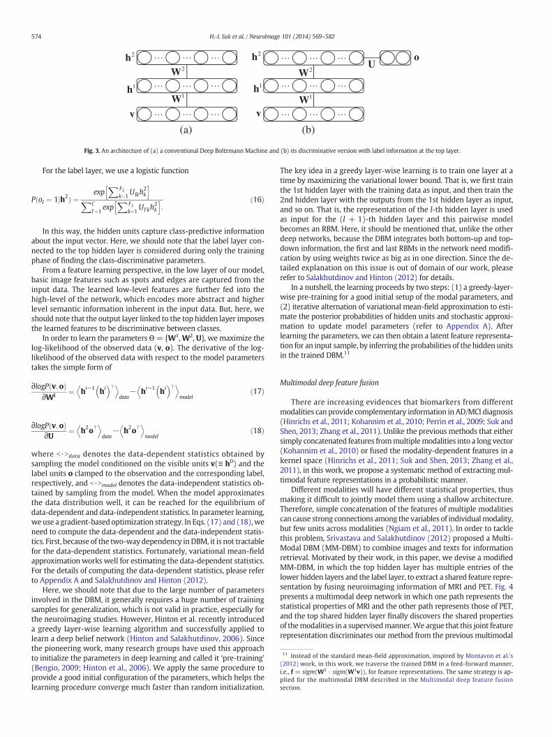
Fig. 3(a) shows an example of the three-layer DBM. The energy ofthe state (v, h1, h2) in the DBM is given by

E v;h1;h2

;Θ� �

¼ −v⊤W1h1− h1� �⊤

W2h2 ð8Þ

where W1 ¼ W1ij

h i∈RD� F1 and W2 ¼ W2

jk

h i∈RF1�F2 are, respectively,

symmetric connections of (v, h1) and (h1, h2), and Θ = {W1, W2}.Then the probability that the model assigns to a visible vector v isgiven by:

P v;Θð Þ ¼ 1Z Θð Þ

Xh1 ;h2

exp −E v;h1;h2

;� �� �

ð9Þ

where Z(Θ) is a normalizing factor. Given the values of the units in theneighboring layer(s), the probability of the binary visible or binary hiddenunits being set to 1 is computed as follows:

P h1j ¼ 1� ���v;h2

�¼ sigm

XDi¼1

W1ijvi þ

XF2k¼1

W2jkh

2k

!ð10Þ

P h2k ¼ 1� ���h1

�¼ sigm

XF1j¼1

W2jkh

1j

0@ 1A ð11Þ

P vi ¼ 1ð jh1Þ ¼ sigmXF1j¼1

W1ijh

1j

0@ 1A: ð12Þ

Note that in the computation of the probability of the hidden unitsh1, we incorporate both the lower visible layer v and the higher hiddenlayer h2, and this makes DBM differentiated from other deep learningmodels and also more robust to noisy observations (Salakhutdinovand Hinton, 2009; Srivastava and Salakhutdinov, 2012).

Unlike the conventional generative DBM, in this work, we consider adiscriminative DBM, by injecting a discriminative RBM (Larochelle andBengio, 2008) at the top hidden layer. That is, the top hidden layer isconnected to both the lower hidden layer and the additional labellayer (Fig. 3(b)), which indicates the label of the input v. In this way,we can train DBM to discover hierarchical and discriminative featurerepresentations by integrating the process of discovering features of in-puts with their use in classification (Larochelle and Bengio, 2008). Ourmodel does not require an additional fine-tuning step for classificationas done in Ngiam et al. (2011) and Salakhutdinov and Hinton (2009).With the inclusion of the additional label layer, the energy of the state(v, h1, h2, o) in the modified DBM is given by

E v;h1;h2

;o;Θ� �

¼ −v⊤W1h1− h1� �⊤

W2h2− h2� �⊤

Uo ð13Þ

whereU ¼ Ulk½ �∈RC� F2 and o= [ol]∈ {0,1}C denote, respectively, a con-nectivity between the top hidden layer and the label layer and a class-label indicator vector, C is the number of classes, and Θ = {W1, W2, U}.The probability of an observation (v, o) is computed by

P v;o;Θð Þ ¼ 1Z Θð Þ

Xh1 ;h2

exp −E v;h1;h2

;o;� �� �

: ð14Þ

The conditional probability of the top hidden units being set to 1 isgiven by

P h2k ¼ 1� ���h1

;o�¼ sigm

XF1j¼1

W2jkh

1j þ

XCl¼1

Ulkol

0@ 1A: ð15Þ

11 Instead of the standard mean-field approximation, inspired by Montavon et al.'s(2012) work, in this work, we traverse the trained DBM in a feed-forward manner,i.e., f = sigm(W2 · sigm(W1v)), for feature representations. The same strategy is ap-plied for the multimodal DBM described in the Multimodal deep feature fusionsection.

(a) (b)

Fig. 3. An architecture of (a) a conventional Deep Boltzmann Machine and (b) its discriminative version with label information at the top layer.

574 H.-I. Suk et al. / NeuroImage 101 (2014) 569–582

For the label layer, we use a logistic function

P ol ¼ 1ð jh2Þ ¼exp

XF2k¼1

Ulkh2k

h iXC

l0¼1exp

XF2k¼1

Ul0kh2k

h i:

ð16Þ

In this way, the hidden units capture class-predictive informationabout the input vector. Here, we should note that the label layer con-nected to the top hidden layer is considered during only the trainingphase of finding the class-discriminative parameters.

From a feature learning perspective, in the low layer of our model,basic image features such as spots and edges are captured from theinput data. The learned low-level features are further fed into thehigh-level of the network, which encodes more abstract and higherlevel semantic information inherent in the input data. But, here, weshould note that the output layer linked to the top hidden layer imposesthe learned features to be discriminative between classes.

In order to learn the parameters Θ= {W1,W2, U}, we maximize thelog-likelihood of the observed data (v, o). The derivative of the log-likelihood of the observed data with respect to the model parameterstakes the simple form of

∂logP v;oð Þ∂Wi

¼ hi−1 hi� �⊤D E

data− hi−1 hi

� �⊤D Emodel

ð17Þ

∂logP v;oð Þ∂U ¼ h2o⊤

D Edata

− h2o⊤D E

modelð18Þ

where b·Ndata denotes the data-dependent statistics obtained bysampling the model conditioned on the visible units v(≡ h0) and thelabel units o clamped to the observation and the corresponding label,respectively, and b·Nmodel denotes the data-independent statistics ob-tained by sampling from the model. When the model approximatesthe data distribution well, it can be reached for the equilibrium ofdata-dependent and data-independent statistics. In parameter learning,we use a gradient-based optimization strategy. In Eqs. (17) and (18),weneed to compute the data-dependent and the data-independent statis-tics. First, because of the two-waydependency inDBM, it is not tractablefor the data-dependent statistics. Fortunately, variational mean-fieldapproximation works well for estimating the data-dependent statistics.For the details of computing the data-dependent statistics, please referto Appendix A and Salakhutdinov and Hinton (2012).

Here, we should note that due to the large number of parametersinvolved in the DBM, it generally requires a huge number of trainingsamples for generalization, which is not valid in practice, especially forthe neuroimaging studies. However, Hinton et al. recently introduceda greedy layer-wise learning algorithm and successfully applied tolearn a deep belief network (Hinton and Salakhutdinov, 2006). Sincethe pioneering work, many research groups have used this approachto initialize the parameters in deep learning and called it ‘pre-training’(Bengio, 2009; Hinton et al., 2006). We apply the same procedure toprovide a good initial configuration of the parameters, which helps thelearning procedure converge much faster than random initialization.

The key idea in a greedy layer-wise learning is to train one layer at atime by maximizing the variational lower bound. That is, we first trainthe 1st hidden layer with the training data as input, and then train the2nd hidden layer with the outputs from the 1st hidden layer as input,and so on. That is, the representation of the l-th hidden layer is usedas input for the (l + 1)-th hidden layer and this pairwise modelbecomes an RBM. Here, it should be mentioned that, unlike the otherdeep networks, because the DBM integrates both bottom-up and top-down information, the first and last RBMs in the network need modifi-cation by using weights twice as big as in one direction. Since the de-tailed explanation on this issue is out of domain of our work, pleaserefer to Salakhutdinov and Hinton (2012) for details.

In a nutshell, the learning proceeds by two steps: (1) a greedy-layer-wise pre-training for a good initial setup of the modal parameters, and(2) iterative alternation of variational mean-field approximation to esti-mate the posterior probabilities of hidden units and stochastic approxi-mation to update model parameters (refer to Appendix A). Afterlearning the parameters, we can then obtain a latent feature representa-tion for an input sample, by inferring the probabilities of thehidden unitsin the trained DBM.11

Multimodal deep feature fusion

There are increasing evidences that biomarkers from differentmodalities can provide complementary information in AD/MCI diagnosis(Hinrichs et al., 2011; Kohannim et al., 2010; Perrin et al., 2009; Suk andShen, 2013; Zhang et al., 2011). Unlike the previous methods that eithersimply concatenated features frommultiplemodalities into a long vector(Kohannim et al., 2010) or fused the modality-dependent features in akernel space (Hinrichs et al., 2011; Suk and Shen, 2013; Zhang et al.,2011), in this work, we propose a systematic method of extracting mul-timodal feature representations in a probabilistic manner.

Different modalities will have different statistical properties, thusmaking it difficult to jointly model them using a shallow architecture.Therefore, simple concatenation of the features of multiple modalitiescan cause strong connections among the variables of individualmodality,but few units across modalities (Ngiam et al., 2011). In order to tacklethis problem, Srivastava and Salakhutdinov (2012) proposed a Multi-Modal DBM (MM-DBM) to combine images and texts for informationretrieval. Motivated by their work, in this paper, we devise a modifiedMM-DBM, in which the top hidden layer has multiple entries of thelower hidden layers and the label layer, to extract a shared feature repre-sentation by fusing neuroimaging information of MRI and PET. Fig. 4presents a multimodal deep network in which one path represents thestatistical properties of MRI and the other path represents those of PET,and the top shared hidden layer finally discovers the shared propertiesof themodalities in a supervisedmanner.We argue that this joint featurerepresentation discriminates our method from the previous multimodal

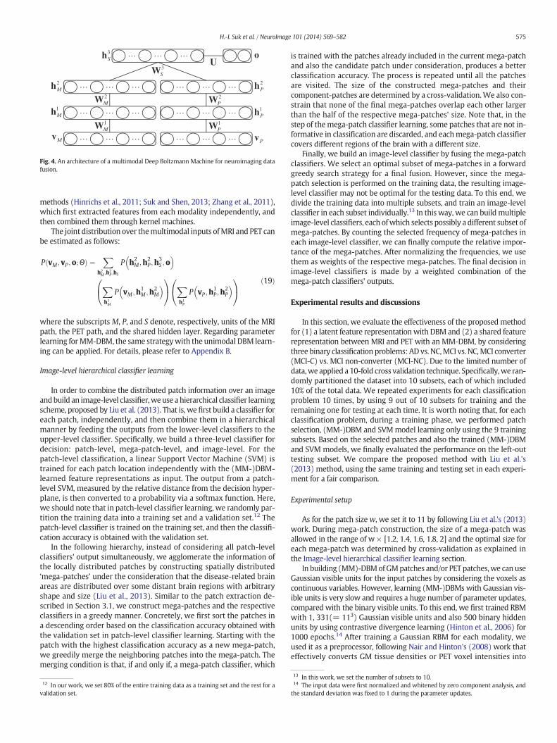
Fig. 4. An architecture of a multimodal Deep Boltzmann Machine for neuroimaging datafusion.

575H.-I. Suk et al. / NeuroImage 101 (2014) 569–582

methods (Hinrichs et al., 2011; Suk and Shen, 2013; Zhang et al., 2011),which first extracted features from each modality independently, andthen combined them through kernel machines.

The joint distribution over themultimodal inputs ofMRI and PET canbe estimated as follows:

P vM; vP ;o;Θð Þ ¼X

h2M ;h2

P ;hS

P h2M ;h

2P ;h

3S ;o

� �Xh1M

P vM ;h1M ;h

2M

� �0@ 1A Xh1P

P vP ;h1P ;h

2P

� �0@ 1A ð19Þ

where the subscripts M, P, and S denote, respectively, units of the MRIpath, the PET path, and the shared hidden layer. Regarding parameterlearning forMM-DBM, the same strategywith the unimodal DBM learn-ing can be applied. For details, please refer to Appendix B.

Image-level hierarchical classifier learning

In order to combine the distributed patch information over an imageandbuild an image-level classifier,weuse ahierarchical classifier learningscheme, proposed by Liu et al. (2013). That is, we first build a classifier foreach patch, independently, and then combine them in a hierarchicalmanner by feeding the outputs from the lower-level classifiers to theupper-level classifier. Specifically, we build a three-level classifier fordecision: patch-level, mega-patch-level, and image-level. For thepatch-level classification, a linear Support Vector Machine (SVM) istrained for each patch location independently with the (MM-)DBM-learned feature representations as input. The output from a patch-level SVM, measured by the relative distance from the decision hyper-plane, is then converted to a probability via a softmax function. Here,we should note that in patch-level classifier learning, we randomly par-tition the training data into a training set and a validation set.12 Thepatch-level classifier is trained on the training set, and then the classifi-cation accuracy is obtained with the validation set.

In the following hierarchy, instead of considering all patch-levelclassifiers' output simultaneously, we agglomerate the information ofthe locally distributed patches by constructing spatially distributed‘mega-patches’ under the consideration that the disease-related brainareas are distributed over some distant brain regions with arbitraryshape and size (Liu et al., 2013). Similar to the patch extraction de-scribed in Section 3.1, we construct mega-patches and the respectiveclassifiers in a greedy manner. Concretely, we first sort the patches ina descending order based on the classification accuracy obtained withthe validation set in patch-level classifier learning. Starting with thepatch with the highest classification accuracy as a new mega-patch,we greedily merge the neighboring patches into the mega-patch. Themerging condition is that, if and only if, a mega-patch classifier, which

12 In our work, we set 80% of the entire training data as a training set and the rest for avalidation set.

is trained with the patches already included in the current mega-patchand also the candidate patch under consideration, produces a betterclassification accuracy. The process is repeated until all the patchesare visited. The size of the constructed mega-patches and theircomponent-patches are determined by a cross-validation.We also con-strain that none of the final mega-patches overlap each other largerthan the half of the respective mega-patches' size. Note that, in thestep of themega-patch classifier learning, some patches that are not in-formative in classification are discarded, and eachmega-patch classifiercovers different regions of the brain with a different size.

Finally, we build an image-level classifier by fusing the mega-patchclassifiers. We select an optimal subset of mega-patches in a forwardgreedy search strategy for a final fusion. However, since the mega-patch selection is performed on the training data, the resulting image-level classifier may not be optimal for the testing data. To this end, wedivide the training data into multiple subsets, and train an image-levelclassifier in each subset individually.13 In this way, we can buildmultipleimage-level classifiers, each ofwhich selects possibly a different subset ofmega-patches. By counting the selected frequency of mega-patches ineach image-level classifier, we can finally compute the relative impor-tance of the mega-patches. After normalizing the frequencies, we usethem as weights of the respective mega-patches. The final decision inimage-level classifiers is made by a weighted combination of themega-patch classifiers' outputs.

Experimental results and discussions

In this section, we evaluate the effectiveness of the proposed methodfor (1) a latent feature representationwith DBM and (2) a shared featurerepresentation between MRI and PET with an MM-DBM, by consideringthree binary classification problems: ADvs. NC,MCI vs. NC,MCI converter(MCI-C) vs. MCI non-converter (MCI-NC). Due to the limited number ofdata,we applied a 10-fold cross validation technique. Specifically,we ran-domly partitioned the dataset into 10 subsets, each of which included10% of the total data. We repeated experiments for each classificationproblem 10 times, by using 9 out of 10 subsets for training and theremaining one for testing at each time. It is worth noting that, for eachclassification problem, during a training phase, we performed patchselection, (MM-)DBM and SVMmodel learning only using the 9 trainingsubsets. Based on the selected patches and also the trained (MM-)DBMand SVM models, we finally evaluated the performance on the left-outtesting subset. We compare the proposed method with Liu et al.'s(2013) method, using the same training and testing set in each experi-ment for a fair comparison.

Experimental setup

As for the patch size w, we set it to 11 by following Liu et al.'s (2013)work. During mega-patch construction, the size of a mega-patch wasallowed in the range of w × [1.2, 1.4, 1.6, 1.8, 2] and the optimal size foreach mega-patch was determined by cross-validation as explained inthe Image-level hierarchical classifier learning section.

In building (MM)-DBMof GMpatches and/or PET patches, we can useGaussian visible units for the input patches by considering the voxels ascontinuous variables. However, learning (MM-)DBMs with Gaussian vis-ible units is very slow and requires a huge number of parameter updates,compared with the binary visible units. To this end, we first trained RBMwith 1, 331(= 113) Gaussian visible units and also 500 binary hiddenunits by using contrastive divergence learning (Hinton et al., 2006) for1000 epochs.14 After training a Gaussian RBM for each modality, weused it as a preprocessor, following Nair and Hinton's (2008) work thateffectively converts GM tissue densities or PET voxel intensities into

13 In this work, we set the number of subsets to 10.14 The input data were first normalized and whitened by zero component analysis, andthe standard deviation was fixed to 1 during the parameter updates.

576 H.-I. Suk et al. / NeuroImage 101 (2014) 569–582

500-dimensional binary vectors. We then used the binary vectors as‘preprocessed data’ to train our (MM-)DBMs. We should note that theGaussian RBMs were not updated during (MM-)DBM learning.

We structured a three-layer DBM for MRI (MRI-DBM) and PET(PET-DBM), respectively, and a four-layer DBM for MRI + PET(MM-DBM). For all these models, we used binary visible and binaryhidden units. Both the MRI-DBM and the PET-DBM were structuredwith 500(visible)–500(hidden)–500(hidden), and the MM-DBMwas structured with 500(visible)–500(hidden)–500(hidden) for aMRI pathway, 500(visible)–500(hidden)–500(hidden) for a PETpathway, and finally 1000 hidden units for the shared hidden layer.In (MM-)DBM learning, we updated the parameters, i.e., weightsand biases, with a learning rate of 10–3 and a momentum of 0.5with an increment gradually up to 0.9 for 500 epochs. We used thetrained parameters of MRI-DBM and PET-DBM as the initial setupof the MRI and PET pathways in MM-DBM learning. We implement-ed the DBM method based on Salakhutdinov's codes.15

We used a linear SVM for the hierarchical classifiers, i.e., patch-levelclassifier, mega-patch-level classifier, and image-level classifier. AnLIBSVM toolbox16 was used for SVM learning and classification. Thefree parameter that controls the soft margin was determined by anested cross-validation.

Extracted patches and trained DBMs

In Fig. 5, we presented the example images overlaid with p-values ofthevoxels, obtained fromADandNCgroups, based onwhichwe selectedpatch locations for AD and NC classification. It is worth noting that, forboth modalities, the voxels in the subcortical and medial temporalareas showed low p-values, i.e., statistically different between classes,while for other areas, each modality presents slightly different p-valuedistributions, from which we could possibly obtain complementary in-formation for classification. Samples of the selected 3D patches are alsopresented in Fig. 6, in which one 3D volume is displayed in each row,for each modality. Taking these patches as input data to a GaussianRBM and then transforming to binary vectors, we trained our featurerepresentationmodels, i.e., MRI-DBM, PET-DBM, andMM-DBM. Regard-ing the trained MM-DBM, we visualized the trained weights in Fig. 7 bylinearly projecting them to the input space for intuitive interpretation ofthe feature representations.17 In the figure, the left images represent thetrainedweights of our Gaussian RBMs thatwere used to convert the real-valued patches into binary vectors as a preprocessor, and the rightimages represent the trained weights of the first-layer hidden units ofthe respective modality's pathway in our MM-DBM. From the figure,we can regard the hidden units in the Gaussian RBM as simple cells ofa human visual cortex that maximally responds to specific spot- oredge-like stimulus patterns within the receptive field, i.e., a patch inour case. In particular, each hidden unit in a Gaussian RBM finds simplevolumetric or functional patterns in the input 3D patch by assigning dif-ferent weights to the corresponding voxels. For example, hidden units ofthe Gaussian RBM for MRI (left in Fig. 7(a)) focus on different parts of apatch to detect a simple spot- or edge-like pattern in the input 3D GMpatch. The hidden units in a Gaussian RBM for PET (left in Fig. 7(b))can be understood as descriptors that discover local functional relationsamong voxels within a patch.

Note that the hidden units of a Gaussian RBM for either MRI or PETfind, respectively, the structural or functional relations among voxels ina localized way. Meanwhile, the hidden units in our (MM-)DBM servedas complex filters of a human visual cortex that combine the outputsfrom the simple cells andmaximally responds tomore complex patterns

15 Available at ‘http://www.cs.toronto.edu/rsalakhu/DBM.html’.16 Available at ‘http://www.csie.ntu.edu.tw/cjlin/libsvm/’.17 For the hidden units of theMRI pathway and the PET pathway, their weights were vi-sualized as a weighted linear combination of the weights of the Gaussian RBM, similar toLee et al.'s (2009) work.

within the receptive field. For example, the weights of hidden units inthe hidden layer of the MRI pathway in an MM-DBM (right inFig. 7(a)) discover more complicated structural patterns in the input3D GM patch, such as combination of edges orienting in different direc-tions. With respect to the PET, the weights of hidden units in the hiddenlayer of the PET pathway in an MM-DBM (right in Fig. 7(b)) discovernon-linear functional relations among voxels within a 3D patch. In thisway, as it forwards to the higher layer, the MM-DBM finds complexlatent features in the input patch, and ultimately in the top hiddenlayer, the hidden units discover the inter-modality relations in betweenthe pair of MRI and PET patches, each of which comes from the same lo-cation in a brain.

Performance evaluation

Let TP, TN, FP, and FN denote, respectively, True Positive, TrueNegative, False Positive, and False Negative. In this work, we considerthe following quantitative measurements and presented the perfor-mances of the competing methods in Table 2.

• ACCuracy (ACC) = (TP + TN) / (TP + TN+ FP + FN)• SENsitivity (SEN) = TP / (TP + FN)• SPECificity (SPEC) = TN / (TN + FP)• Balanced ACcuracy (BAC) = (SEN + SPEC) / 2• Positive Predictive Value (PPV) = TP / (TP + FP)• Negative Predictive Value (NPV) = TN / (TN + FN)• Area Under the receiver operating characteristic Curve (AUC)

In the classification of AD and NC, the proposed method showedthe mean accuracies of 92.38% (MRI), 92.20% (PET), and 95.35%(MRI+ PET). Compared to Liu et al.'smethod that showed the accuraciesof 90.18% (MRI), 89.13% (PET), and 90.27% (MRI + PET),18 the proposedmethod improved by 2.2% (MRI), 3.07% (PET), and 5.08% (MRI + PET).That is, the proposed method outperformed Liu et al.'s method in all thecases of MRI, PET, and MRI + PET. In the discrimination of MCI fromNC, the proposed method showed the accuracies of 84.24% (MRI),84.29% (PET), and 85.67% (MRI + PET). Meanwhile, Liu et al.'s methodshowed the accuracies of 81% (MRI), 81.14% (PET), and 83.90%(MRI + PET). Again, the proposed method outperformed Liu et al.'smethod by making performance improvements of 3.24% (MRI),3.15% (PET), and 1.77% (MRI + PET). In the classification betweenMCI-C and MCI-NC, which is the most important for early diagnosisand treatment, Liu et al.'s method achieved the accuracies of 64.75%(MRI), 67.17% (PET), and 73.33% (MRI + PET). Compared to these re-sults, the proposed method improved the accuracies by 7.67% (MRI),3.58% (PET), and 2.59% (MRI + PET), respectively. Concisely, in ourthree binary classifications, based on the classification accuracy, theproposedmethod clearly outperformed Liu et al.'s method by achievingthemaximal accuracies of 95.35% (AD vs. NC), 85.67% (MCI vs. NC), and75.92% (MCI-C vs. MCI-NC), respectively.

Regarding sensitivity and specificity, the higher the sensitivity, thelower the chance of mis-diagnosing AD/MCI patients; also the higherthe specificity, the lower the chance of mis-diagnosing NC to AD/MCI.Although the proposed method had a lower sensitivity than that of Liuet al.'s method for a couple of cases, e.g., 90.06% (Liu et al.'s method)vs. 88.04% (proposed) with PET in the AD diagnosis, 98.97% (Liuet al.'s method) vs. 95.37% (proposed) with MRI+ PET in theMCI diag-nosis, and 40.02% (Liu et al.'smethod) vs. 25.45% (proposed)with PET inthe MCI-C diagnosis, in general, the proposed method showed highersensitivity and specificity in all three classification problems. Hence,from a clinical point of view, the proposed method is less likely tomis-diagnose subjects with AD/MCI and vice versa, compared to Liuet al.'s method.

18 For themultimodal case, we concatenated the patches of modalities into a single vec-tor for Liu et al.'s method.

(a) MRI

(b) PET

Fig. 5. Visualization of the p-value distributions used to select the patch locations of MRI and PET in AD and NC classification.

577H.-I. Suk et al. / NeuroImage 101 (2014) 569–582

Meanwhile, because of the data imbalance between classes, i.e., AD(93 subjects), MCI (204 subjects; 76 MCI-C and 128 MCI-NC subjects),andNC (101 subjects),we obtained low sensitivity (MCI vs. NC) or spec-ificity (MCI-C vs. MCI-NC). The balanced accuracy, which is calculatedby taking the average of sensitivity and specificity, avoids inflated

(a) MRI

Fig. 6. Samples of the selected patches, whose vo

performance estimates on imbalanced datasets. Based on this metric,we clearly see that the proposed method is superior to the competingmethod. Note that in discrimination between MCI and NC, while theaccuracy improvement by the proposed method with MRI + PET was1.43% and 1.38% compared to the same method with MRI and PET,

(b) PET

xel values are the input to the (MM-)DBM.

(a) MRI

(b) PET

Fig. 7. Visualization of the trained weights of our modality-specific Gaussian RBMs (left) used for data conversion from a real-valued vector to a binary vector, and those of our MM-DBM(right) used for latent feature representations. For the weights of our MM-DBM, they correspond to the first hidden layer in the respective modality's pathway in the model. In eachsubfigure, one row corresponds to one hidden unit in the respective Gaussian RBM or MM-DBM.

578 H.-I. Suk et al. / NeuroImage 101 (2014) 569–582

respectively, in terms of the balanced accuracy, the improvements wentup to 3.93% (vs. MRI) and 2.95% (vs. PET).

With a further concern on low sensitivity and specificity, especiallyin classifications of MCI vs. NC andMCI-C vs.MCI-NC,we also computed

Table 2A summary of the performances of two methods. The boldface denotes the best performance i

Method Modality ACC (%) SEN (

AD/NC Liu et al. MRI 90.18 ± 5.25 91.54PET 89.13 ± 6.81 90.06MRI + PET 90.27 ± 7.02 89.48

Proposed MRI 92.38 ± 5.32 91.54PET 92.20 ± 6.70 88.04MRI + PET 95.35 ± 5.23 94.65

MCI/NC Liu et al. MRI 81.00 ± 4.98 97.08PET 81.14 ± 10.22 96.03MRI + PET 83.90 ± 5.80 98.97

Proposed MRI 84.24 ± 6.26 99.58PET 84.29 ± 7.22 98.69MRI + PET 85.67 ± 5.22 95.37

MCI-C/MCI-NC Liu et al. MRI 64.75 ± 14.83 22.22PET 67.17 ± 13.43 40.02MRI + PET 73.33 ± 12.47 33.25

Proposed MRI 72.42 ± 13.09 36.70PET 70.75 ± 13.23 25.45MRI + PET 75.92 ± 15.37 48.04

a Positive Predictive Value (PPV) and a Negative Predictive Value (NPV).Statistically, PPV and NPV measure, respectively, the proportion of sub-jects with AD, MCI, or MCI-C who are correctly diagnosed as patients,and the proportion of subjects without AD, MCI, or MCI-C who are

n each metric for each classification task.

%) SPEC (%) BAC (%) PPV (%) NPV (%) AUC (%)

90.61 91.08 88.94 90.67 0.962089.36 89.71 88.49 89.26 0.959492.44 90.96 90.56 88.70 0.965594.56 93.05 92.65 90.84 0.969796.33 92.19 95.03 89.66 0.979895.22 94.93 96.80 95.67 0.987748.18 72.63 79.14 88.99 0.835252.59 74.31 80.26 84.16 0.823152.59 75.78 81.18 97.22 0.830153.79 76.69 81.23 98.75 0.847856.87 77.78 81.99 94.57 0.829765.87 80.62 85.02 89.00 0.880889.57 55.90 46.29 77.39 0.635582.61 61.32 64.13 70.31 0.691197.52 65.38 80.00 73.18 0.715990.98 63.84 65.49 77.84 0.734296.55 61.00 75.00 70.69 0.721595.23 71.63 83.50 74.33 0.7466

579H.-I. Suk et al. / NeuroImage 101 (2014) 569–582

correctly diagnosed as cognitive normal. Based on a recent report byAlzheimer's Association (2012), the AD prevalence is projected to be11 million to 16 million by 2050. For MCI and MCI-C, although there ishigh variation among reports depending on definitions, the median ofthe prevalence estimates of MCI or MCI-C in the literature is 26.4%(MCI) and 4.9% (amnestic MCI) (Ward et al., 2012). Regarding the ADprevalence by 2050, the proposed method, which achieved 96.80% ofthe PPV in the classification of AD and NC, can correctly identify10.648 million to 15.488 million of subjects with AD while Liu et al.'smethod, whose respective PPV was 90.56%, can identify 9.9616 millionto 14.4896 million of subjects with AD. Accordingly, our method cancorrectly identify as many as 0.6864 million to 0.9984 million of sub-jects more.

The Receiver Operating Characteristic (ROC) curve19 and the AreaUnder the ROC Curve (AUC) are also widely used metrics to evaluatethe performance of diagnostic tests in brain disease as well as othermedical areas. In particular, the AUC can be thought as a measure ofthe overall performance of a diagnostic test. The proposed methodwith MRI + PET showed the best AUCs of 0.9877 in AD vs. NC, 0.8808in MCI vs. NC, and 0.7466 in MCI-C vs. MCI-NC. Compared to Liu et al.'smethod with MRI + PET, the proposed multimodal method increasedthe AUCs by 0.0222 (AD vs. NC), 0.0507 (MCI vs. NC), and 0.0307(MCI-C vs. MCI-NC). Noticeably, the proposed method with MRI en-hanced the AUC as much as 0.0987 than the corresponding AUC of Liuet al.'s method. It is also noteworthy that in the classification of MCIand NC, the proposed method with MRI + PET improved the AUC by0.0330 (vs. MRI) and 0.0389 (vs. PET), while the improvements in theclassifications of AD vs. NC and MCI-C vs. MCI-NC were, respectively,0.0180/0.0079 (vs. MRI/PET) and 0.0124/0.0251 (vs. MRI/PET).

Based on the quantitative measurements depicted above, theproposed method clearly outperforms Liu et al.'s method. In termsof modalities used for classification, similar to the previous work(Hinrichs et al., 2011; Suk and Shen, 2013; Zhang et al., 2011), we alsoobtained the best performances with the complementary informationfrom multiple modalities, i.e., MRI + PET.

Comparison with State-of-the-Art Methods

In Table 3, we also compared the classification accuracies of theproposed method with those of the state-of-the-art methods that con-sidered multi-modality in classifications of AD vs. NC, MCI vs. NC, andMCI-C vs. MCI-NC. Note that, due to different datasets and differentapproaches of extracting features and building classifiers, it is not fairto directly compare the performances among methods. Nonetheless, itis remarkable that the proposedmethod showed the highest accuraciesamong the methods in all the binary classification problems. It is alsoworth noting that our method is the only one that considered thepatch-based approach for feature extraction, while the other methodsused an ROI-based approach.

Importance of brain areas in classification

For the investigation of the relative importance of different brainareas determined by the proposed method for AD/MCI diagnosis, wevisualized the weights of the selected patches in Fig. 8. Specifically, theweight of each patch was calculated by accumulating the selectedfrequency of mega-patches in final ensemble classifiers over cross-validations. That is, the weight of a patch was determined with thesum of the weights of the mega-patches that included the patchand was used in the final decision. The high weighted patches werein accordance with the previous reports on AD/MCI studies. Thosewere distributed around a medial temporal lobe (that includesamygdala, hippocampal formation, entorhinal cortex) (Braak and

19 A plot of test true positive rate versus its false positive rate.

Braak, 1991; Burton et al., 2009; Desikan et al., 2009; Devanand et al.,2007; Ewers et al., 2012; Lee et al., 2006; Mosconi, 2005; Visser et al.,2002; Walhovd et al., 2010), superior/medial frontal gyrus (Johnsonet al., 2005), precentral/postcentral gyrus (Belleville et al., 2011),precuneus (Bokde et al., 2006; Davatzikos et al., 2011; Singh et al.,2006), thalamus, putamen (de Jong et al., 2008), caudate nucleus (Daiet al., 2009), etc.

Limitations

In our experiments, we validated the efficacy of the proposedmethod in three classification problems by achieving the best perfor-mances. However, there still exist some limitations of the proposedmethod.

First, even though we could visualize the trained weights in ourMM-DBMs in Fig. 7, from a clinical perspective, it is difficult to under-stand or interpret the resulting feature representations. Particularly,with respect to the investigation of brain abnormalities affected byneurodegenerative disease, i.e., AD or MCI, our method cannot provideuseful clinical information. In this regard, it could be a good researchdirection in which we further extend the proposed method to find ordetect brain abnormalities in terms of brain regions or areas for easy un-derstanding to clinicians.

Second, in our experiments, wemanually determined the number ofhidden units in each layer. Furthermore, we used a relatively small datasamples (93 AD, 76 MCI-C, 128 MCI-NC, and 101 NC). Therefore, thenetwork structures used to discover high-level feature representationsin our experiments were not necessarily optimal. We believe that itneeds more intensive studies such as learning the optimal networkstructure from big data for practical use of deep learning in clinicalsettings.

Third, as the graphicalmodel illustrated in Fig. 4, the currentmethodonly considers bi-modalities of MRI and PET. However, it is generallybeneficiary to combine asmanymodalities as possible to use their richerinformation. Therefore, it is necessary to build amore systematic modelthat can efficiently find and use complementary information fromgenetics, proteomics, imaging, cognition, disease status, and other phe-notypic modalities.

Lastly, according to a recent broad spectrum of studies, there areincreasing evidences that subjective cognitive complaint is one of theimportant genetic risk factors, which increases the risk of progressionto MCI or AD (Loewenstein et al., 2012; Mark and Sitskoorn, 2013).That is, among the cognitively normal elderly individualswhohave sub-jective cognitive impairments, there exists a high possibility for some ofthem to be in the stage of ‘pre-MCI’. However, in the ADNI dataset, thereis no related information. Thus, in our experiments, the NC group couldinclude both genuine controls and those with subjective cognitivecomplaints.

Conclusions

In this paper, we proposed a method for a shared latent featurerepresentation from MRI and PET in deep learning. Specifically, weused DBM to find a latent feature representation from a volumetricpatch and further devised method to systemically discover a joint fea-ture representation from multi-modality. Unlike the previous methodsthat mostly considered the direct use of the GM tissue densities fromMRI and/or voxel intensities from PET and then fused the complemen-tary information in a kernel technique, the proposed method learnedhigh-level features in a self-taught manner via deep learning, and thuscould efficiently combine the complimentary information from MRIand PET during feature representation procedure. Experimental resultson ADNI dataset showed that the proposed method is superior to theprevious methods in terms of various quantitative metrics.

Table 3Comparison of classification accuracywith state-of-the-art methods. The numbers in the parentheses denote the number of AD/MCI(MCI-C, MCI-NC)/NC subjects in the dataset used. Theboldface denotes the best performance in each classification task.

Methods Dataset Features AD vs. NC (%) MCI vs. NC (%) MCI-C vs. MCI-NC (%)

Kohannim et al. (2010) MRI + PET + CSF (40/83(43,40)/43) ROI 90.7 75.8 n/aWalhovd et al. (2010) MRI + CSF (38/73/42) ROI 88.8 79.1 n/aHinrichs et al. (2011) MRI + PET (48/119(38,81)/66) ROI 92.4 n/a 72.3Westman et al. (2012) MRI + CSF (96/162(81,81)/111) ROI 91.8 77.6 66.4Zhang and Shen (2012) MRI + PET + CSF (45/91(43,48)/50) ROI 93.3 83.2 73.9Proposed method MRI + PET (93/204(76,128)/101) Patch 95.35 85.67 75.92

580 H.-I. Suk et al. / NeuroImage 101 (2014) 569–582

Acknowledgment

This work was supported in part by NIH grants EB006733, EB008374,EB009634, AG041721, MH100217, and AG042599, and also by theNational Research Foundation grant (No. 2012-005741) funded by theKorean Government.

Appendix A. Variational approximation for DBM learning

The main idea of applying variational approximation is to assumethat the true posterior distribution over latent variables P(h1, h2 | v; Θ)for each training vector v is unimodal and can be replaced by an

(a) AD vs. NC

(c) MCI-C vs

Fig. 8. Patch weight distributions in classi

approximate posteriorQ(h1,h2 | v;Ω),which can be computed efficient-ly, and the parameters are updated to maximize the variational lowerbound on the log-likelihood

logP v;Θð Þ≥Xh1 ;h2

Q h1;h2

� ���v;�logP v;h1;h2

;Θ� �

þ H Qð Þ ðA:1Þ

¼ logP v;Θð Þ−KL Q h1;h2

� ���v;Ωh �kP h1

;h2� ���v;Θj�i ðA:2Þ

(b) MCI vs. NC

. MCI-NC

fication of AD vs. NC and MCI vs. NC.

581H.-I. Suk et al. / NeuroImage 101 (2014) 569–582

where H(·) is the entropy functional, KL[·||·] denotes Kullback–Leiblerdivergence, and Ω is a variational parameter set.

For computational simplicity and learning speed, the naïve mean-field approximation, which uses a fully factorized distribution, is gener-ally used in the literature (Tanaka, 1998). That is,

Q h1;h2

� ���v;Ω� ¼ ∏F1

j¼1q h1j� �

∏F2

k¼1q h2k� �

ðA:3Þ

whereΩ={μ1,μ2},μ1 ¼ μ11; ⋯; μ

1F1

� �,μ2 ¼ μ2

1; ⋯; μ2F2

� �, q(hj1=1)= μj1

(j ∈ {1,⋯, F1}), and q(hj2 = 1) = μk2 (k ∈ {1,⋯, F2}). It alternatively esti-mates the state of the hidden units, μ1 and μ2, for fixed Θ until conver-gence:

μ1j←sigm

XDi¼1

W1ijvi þ

XF2k¼1

W2jkμ

2k

!ðA:4Þ

μ2k←sigm

XF1j¼1

W2jkμ

1j þ

XCl¼1

Ulkol

0@ 1A: ðA:5Þ

Regarding the data-independent statistics, we apply a stochastic ap-

proximation procedure to obtain samples, also called particles, of ev, eh1,eh2

, and eo by running repeatedly the alternate Gibbs sampler on a set ofparticles. Once both the data-dependent and data-independent statis-tics are computed, we then update parameters as follows:

W1; tþ1ð Þ ¼ W1; tð Þ þ αt1N∑N

n¼1 vnμ1;n⊤− 1

M∑M

m¼1vemhe1;m⊤�

ðA:6Þ

W2; tþ1ð Þ ¼ W2; tð Þ þ αt1N∑N

n¼1μ1;nμ2;n⊤− 1

M∑M

m¼1he1;mhe2;m⊤

� ðA:7Þ

U tþ1ð Þ ¼ U tð Þ þ αt1N∑N

n¼1μ2;non⊤− 1

M∑M

m¼1he2;moen⊤�

ðA:8Þ

where αt is a learning rate, and N and M denote, respectively, thenumbers of trainingdata and particles, and superscripts n andm denote,respectively, indices of an observation and a particle.

Appendix B. Learning multimodal DBM parameters

The same approach to the unimodal DBM described in the DeepBoltzmann Machine section can be applied, i.e., iterative alternation ofthe variational mean-field approximation for data-dependent statisticsand the stochastic approximation procedure for data-independent statis-tics, and parameters update. LetH={hM

1 ,hM2 ,hP

1,hP2,hS

3} andV={vM, vP}.In variational learning of our MM-DBM, a fully factorized mean-fieldvariational function for approximation of the true posterior distributionP(H | V, o; Θ= {WM

1 ,WM2 ,WP

1,WP2,WS

3, U}) is defined as follows:

Q Hð jV;o;ΩÞ ¼ ∏FM1

i¼1q h1M;i

� �∏FM2

j¼1q h2M; j

� �∏FP1

k¼1q h1P;k� �

∏FP2

l¼1q h2P;l� �

∏FS

m¼1q h3S;m� �

¼ ∏FM1

i¼1μ1M;i ∏

FM2

j¼1μ2M; j∏

FP1

k¼1μ1P;k∏

FP2

l¼1μ2P;l ∏

FS

m¼1μ3S;m

ðB:1Þ

where Ω = {μM1 , μM

2 , μP1, μP

2, μS3} is a mean-field parameter set with

μ1M ¼ μ1

M;1; ⋯; μ1M; FM1

� �,μ2

M ¼ μ2M;1; ⋯; μ

2M; FM2

� �,μ1

P ¼ μ1P;1; ⋯; μ

1P;FP1

� �,μ2

P ¼μ2P;1; ⋯; μ

2P; FP2

� �, and μ3

S ¼ μ3S;1; ⋯; μ

3S; FS

� �. Referring Eqs. (A.4) and (A.5),

given a fixed model parameter Θ, it is straightforward to estimate themean-field parameters Ω.

The learning proceeds by iteratively alternating the variationalmean-field inference to find the values of Ω for the fixed currentmodel parametersΘ and the stochastic approximation procedure to up-date model parameters Θ given the variational parameters Ω. Finally,the shared feature representations can be obtained by inferring thevalues of the hidden units in the top hidden layer from the trainedMM-DBM.

References

Alzheimer's Association, 2012. 2012 Alzheimer's disease facts and figures. AlzheimersDement. 8, 131–168.

Baron, J., Chtelat, G.,Desgranges, B., Perchey, G., Landeau, B., de la Sayette, V.,Eustache, F.,2001. In vivo mapping of gray matter loss with voxel-based morphometry in mildAlzheimer's disease. Neuroimage 14, 298–309.

Belleville, S., ClŽment, F.,Mellah, S., Gilbert, B., Fontaine, F., Gauthier, S., 2011. Training-related brain plasticity in subjects at risk of developing Alzheimer's disease. Brain134, 1623–1634.

Bengio, Y., 2009. Learning deep architectures for AI. Foundations and Trends in MachineLearning, 2, pp. 1–127.

Bengio, Y.,Lamblin, P.,Popovici, D.,Larochelle, H., 2007. Greedy layer-wise training of deepnetworks. In: Schölkopf, B., Platt, J., Hoffman, T. (Eds.), Advances in Neural Informa-tion Processing Systems, 19. MIT Press, Cambridge, MA, pp. 153–160.

Bokde, A.L.W.,Lopez-Bayo, P.,Meindl, T.,Pechler, S.,Born, C.,Faltraco, F.,Teipel, S.J.,Möller,H.J.,Hampel, H., 2006. Functional connectivity of the fusiform gyrus during a face-matching task in subjects with mild cognitive impairment. Brain 129, 1113–1124.

Braak, H.,Braak, E., 1991. Neuropathological stageing of Alzheimer-related changes. ActaNeuropathol. 82, 239–259.

Burton, E.J.,Barber, R.,Mukaetova-Ladinska, E.B.,Robson, J.,Perry, R.H.,Jaros, E.,Kalaria, R.N.,OBrien, J.T., 2009. Medial temporal lobe atrophy on MRI differentiates Alzheimer'sdisease from dementia with Lewy bodies and vascular cognitive impairment: a pro-spective study with pathological verification of diagnosis. Brain 132, 195–203.

Catana, C.,Drzezga, A.,Heiss, W.D.,Rosen, B.R., 2012. PET/MRI for neurologic applications.J. Nucl. Med. 53, 1916–1925.

Ciresan, D.C.,Giusti, A.,Gambardella, L.M.,Schmidhuber, J., 2013. Mitosis detection in breastcancer histology images with deep neural networks. Medical Image Computing andComputer-Assisted Intervention MICCAI 2013, pp. 411–418.

Cui, Y., Liu, B., Luo, S., Zhen, X., Fan, M., Liu, T., Zhu, W., Park, M., Jiang, T., Jin, J.S., theAlzheimer's Disease Neuroimaging Initiative, 2011. Identification of conversionfrommild cognitive impairment to Alzheimer's disease using multivariate predictors.PLoS One 6, e21896.

Cuingnet, R., Gerardin, E., Tessieras, J., Auzias, G., Lehéricy, S., Habert, M.O., Chupin, M.,Benali, H.,Colliot, O.,The Alzheimer's Disease Neuroimaging Initiative, 2011. Automaticclassification of patients with Alzheimer's disease from structural MRI: a comparison often methods using ADNI database. Neuroimage 56, 766–781.

Dai, W.,Lopez, O.,Carmichael, O.,Becker, J.,Kuller, L.,Gach, H., 2009. Mild cognitive impair-ment and Alzheimer disease: patterns of altered cerebral blood flow at MR imaging.Radiology 250, 856–866.

Davatzikos, C.,Genc, A.,Xu, D., Resnick, S.M., 2001. Voxel-based morphometry using theRAVENS maps: methods and validation using simulated longitudinal atrophy.Neuroimage 14, 1361–1369.

Davatzikos, C.,Bhatt, P.,Shaw, L.M.,Batmanghelich, K.N.,Trojanowski, J.Q., 2011. Predictionof MCI to AD conversion, via MRI, CSF biomarkers, and pattern classification.Neurobiol. Aging 32 (2322.e19–2322.e27).

de Jong, L.W.,van der Hiele, K.,Veer, I.M.,Houwing, J.J.,Westendorp, R.G.J.,Bollen, E.L.E.M.,de Bruin, P.W.,Middelkoop, H.A.M.,van Buchem,M.A.,van der Grond, J., 2008. Stronglyreduced volumes of putamen and thalamus in Alzheimer's disease: an MRI study.Brain 131, 3277–3285.

Desikan, R.,Cabral, H.,Hess, C.,Dillon, W.,Salat, D., Buckner, R., Fischl, B., Initiative, A.D.N.,2009. Automated MRI measures identify individuals with mild cognitive impairmentand Alzheimer's disease. Brain 132, 2048–2057.

Devanand, D.P.,Pradhaban, G.,Liu, X.,Khandji, A.,De Santi, S.,Segal, S.,Rusinek, H.,Pelton, G.H.,Hoing, L.S.,Mayeux, R.,Stern, Y.,Tabert, M.H.,de Leon, J.J., 2007. Hippocampal and ento-rhinal atrophy in mild cognitive impairment. Neurology 68, 828–836.

Dinov, I.,Boscardin, J.,Mega, M.,Sowell, E.,Toga, A., 2005. A wavelet-based statistical analysisof fMRI data. Neuroinformatics 3, 319–342.

Ewers, M.,Walsh, C., Trojanowski, J.Q., Shaw, L.M., Petersen Jr., R.C., C.R.J., Feldman, H.H.,Bokde, A.L.,Alexander, G.E.,Scheltens, P.,Vellas, B.,Dubois, B.,Weiner, M.,Hampel, H.,2012. Prediction of conversion frommild cognitive impairment toAlzheimer's diseasedementia based upon biomarkers and neuropsychological test performance.Neurobiol. Aging 33, 1203–1214 (e2).

Fan, Y., Rao, H., Hurt, H., Giannetta, J., Korczykowski, M., Shera, D., Avants, B.B., Gee, J.C.,Wang, J., Shen, D., 2007a. Multivariate examination of brain abnormality using bothstructural and functional MRI. Neuroimage 36, 1189–1199.

Fan, Y.,Shen, D.,Gur, R.,Gur, R.,Davatzikos, C., 2007b. COMPARE: classification of morpholog-ical patterns using adaptive regional elements. IEEE Trans. Med. Imaging 26, 93–105.

Friston, K.J., 1995. Functional and effective connectivity in neuroimaging: a synthesis.Hum. Brain Mapp. 2, 56–78.

Greicius, M.D., Srivastava, G.,Reiss, A.L.,Menon, V., 2004. Default-mode network activitydistinguishes Alzheimer's disease from healthy aging: evidence from functionalMRI. Proc. Natl. Acad. Sci. U. S. A. 101, 4637–4642.

Hackmack, K.,Paul, F.,Weygandt, M.,Allefeld, C.,Haynes, J.D., 2012. Multi-scale classifica-tion of disease using structural MRI and wavelet transform. Neuroimage 62, 48–58.

582 H.-I. Suk et al. / NeuroImage 101 (2014) 569–582

Hinrichs, C., Singh, V., Xu, G., Johnson, S.C., 2011. Predictive markers for AD in a multi-modality framework: an analysis of MCI progression in the ADNI population.Neuroimage 55, 574–589.

Hinton, G.E., Salakhutdinov, R.R., 2006. Reducing the dimensionality of data with neuralnetworks. Science 313, 504–507.

Hinton, G.E.,Osindero, S., Teh, Y.W., 2006. A fast learning algorithm for deep belief nets.Neural Comput. 18, 1527–1554.

Hjelm, R.D.,Calhoun, V.D.,Salakhutdinov, R.,Allen, E.A.,Adali, T.,Plis, S.M., 2014. Restrictedboltzmann machines for neuroimaging: an application in identifying intrinsicnetworks. Neuroimage 96, 245–260.

Ishii, K.,Kawachi, T., Sasaki, H.,Kono, A.K., Fukuda, T.,Kojima, Y.,Mori, E., 2005. Voxel-basedmorphometric comparison between early- and late-onset mild Alzheimer's diseaseand assessment of diagnostic performance of z score images. Am. J. Neuroradiol. 26,333–340.

Jia, H.,Wu, G.,Wang, Q.,Shen, D., 2010. ABSORB: atlas building by self-organized registra-tion and bundling. Neuroimage 51, 1057–1070.

Johnson, N.A.,Jahng, G.H.,Weiner, M.W.,Miller, B.L.,Chui, H.C.,Jagust, W.J.,Gorno-Tempini,M.L.,Schuff, N., 2005. Pattern of cerebral hypoperfusion in Alzheimer disease andmildcognitive impairment measured with arterial spin-labeling MR imaging: initial expe-rience. Radiology 234, 851–859.

Kabani, N.,MacDonald, D., Holmes, C., Evans, A., 1998. A 3D atlas of the human brain.Neuroimage 7, S717.

Kohannim, O., Hua, X., Hibar, D.P., Lee, S., Chou, Y.Y., Toga Jr., A.W., C.R.J.,Weiner, M.W.,Thompson, P.M., 2010. Boosting power for clinical trials using classifiers based onmultiple biomarkers. Neurobiol. Aging 31, 1429–1442.

Larochelle, H., Bengio, Y., 2008. Classification using discriminative restricted Boltzmannmachines. Proceedings of the 25th International Conference on Machine Learning,pp. 536–543.

LeCun, Y.,Bottou, L.,Bengio, Y.,Haffner, P., 1998. Gradient-based learning applied to docu-ment recognition. Proc. IEEE 86, 2278–2324.

Lee, A.C.H.,Buckley, M.J.,Gaffan, D.,Emery, T.,Hodges, J.R.,Graham, K.S., 2006. Differentiatingthe roles of the hippocampus and perirhinal cortex in processes beyond long-term de-clarative memory: a double dissociation in dementia. J. Neurosci. 26, 5198–5203.

Lee, H.,Grosse, R., Ranganath, R.,Ng, A.Y., 2009. Convolutional deep belief networks forscalable unsupervised learning of hierarchical representations. Proceedings of the26th International Conference on Machine Learning, pp. 609–616.

Li, Y.,Wang, Y.,Wu, G., Shi, F., Zhou, L., Lin, W., Shen, D., 2012. Discriminant analysis oflongitudinal cortical thickness changes in Alzheimer's disease using dynamic andnetwork features. Neurobiol. Aging 33 (427.e15–427.e30).

Liao, S.,Gao, Y.,Oto, A., Shen, D., 2013. Representation learning: a unified deep learningframework for automatic prostate MR segmentation. Medical Image Computing andComputer-Assisted Intervention MICCAI 2013. Lecture Notes in Computer Science,vol. 8150, pp. 254–261.

Liu, M., Zhang, D., Shen, D., 2012. Ensemble sparse classification of Alzheimer's disease.Neuroimage 60, 1106–1116.

Liu, M.,Zhang, D.,Shen, D., the Alzheimer's Disease Neuroimaging Initiative, 2013. Hierar-chical fusion of features and classifier decisions for Alzheimer's disease diagnosis.Hum. Brain Mapp. 35, 1305–1319.

Loewenstein, D.A.,Greig, M.T.,Schinka, J.A.,Barker, W.,Shen, Q.,Potter, E.,Raj, A.,Brooks, L.,Varon, D., Schoenberg, M., Banko, J., Potter, H., Duara, R., 2012. An investigation ofPreMCI: subtypes and longitudinal outcomes. Alzheimers Dement. 8, 172–179.

Mark, R.E.,Sitskoorn, M.M., 2013. Are subjective cognitive complaints relevant in preclin-ical Alzheimer's disease? A review and guidelines for healthcare professionals. Rev.Clin. Gerontol. 23, 61–74.

Mohamed, A.,Dahl, G.E.,Hinton, G.E., 2012. Acoustic modeling using deep belief networks.IEEE Trans. Audio Speech Lang. Process. 20, 14–22.

Montavon, G.,Braun, M.L.,Möller, K.R., 2012. Deep Boltzmann machines as feed-forward hi-erarchies. Journal of Machine Learning Research—Proceedings Track, 22, pp. 798–804.

Mosconi, L., 2005. Brain glucose metabolism in the early and specific diagnosis ofAlzheimer's disease. Eur. J. Nucl. Med. Mol. Imaging 32, 486–510.

Nair, V.,Hinton, G.E., 2008. Implicit mixtures of restricted Boltzmann machines. Advancesin Neural Information Processing Systems, pp. 1145–1152.

Ngiam, J.,Khosla, A.,Kim, M.,Nam, J.,Lee, H.,Ng, A.Y., 2011. Multimodal deep learning.Proceedings of the 28th International Conference on Machine Learning, pp.689–696.

Nordberg, A.,Rinne, J.O.,Kadir, A.,Langstrom, B., 2010. The use of PET in Alzheimer disease.Nat. Rev. Neurol. 6, 78–87.

Perrin, R.J., Fagan, A.M.,Holtzman, D.M., 2009. Multimodal techniques for diagnosis andprognosis of Alzheimer's disease. Nature 461, 916–922.

Pichler, B.J.,Kolb, A.,Nägele, T.,Schlemmer, H.P., 2010. PET/MRI: paving the way for the nextgeneration of clinical multimodality imaging applications. J. Nucl. Med. 51, 333–336.

Salakhutdinov, R.,Hinton, G.E., 2009. Deep Boltzmannmachines. Proceedings of the Inter-national Conference on Artificial Intelligence and, Statistics, pp. 448–455.

Salakhutdinov, R.,Hinton, G., 2012. An efficient learning procedure for deep Boltzmannmachines. Neural Comput. 24, 1967–2006.

Shen, D.,Davatzikos, C., 2002. HAMMER: hierarchical attribute matching mechanism forelastic registration. IEEE Trans. Med. Imaging 21, 1421–1439.

Shin, H.C.,Orton, M.R.,Collins, D.J.,Doran, S.J.,Leach, M.O., 2013. Stacked autoencoders forunsupervised feature learning and multiple organ detection in a pilot study using 4Dpatient data. IEEE Trans. Pattern Anal. Mach. Intell. 35, 1930–1943.

Singh, V.,Chertkow, H.,Lerch, J.P.,Evans, A.C.,Dorr, A.E.,Kabani, N.J., 2006. Spatial patternsof cortical thinning in mild cognitive impairment and Alzheimer's disease. Brain 129,2885–2893.

Sled, J.G., Zijdenbos, A.P., Evans, A.C., 1998. A nonparametric method for automaticcorrection of intensity nonuniformity in MRI data. IEEE Trans. Med. Imaging17, 87–97.

Srivastava, N., Salakhutdinov, R., 2012. Multimodal learning with deep Boltzmannmachines. Advances in Neural Information Processing Systems, 25, pp. 2231–2239.

Suk, H.I.,Shen, D., 2013. Deep learning-based feature representation for AD/MCI classifica-tion. Medical Image Computing and Computer-Assisted Intervention—MICCAI 2013.Lecture Notes in Computer Science, vol. 8150, pp. 583–590.

Suk, H.I.,Wee, C.Y., Shen, D., 2013. Discriminative group sparse representation for mildcognitive impairment classification. Machine Learning in Medical Imaging. LectureNotes in Computer Science, vol. 8184, pp. 131–138.

Tanaka, T., 1998. A theory of mean field approximation. Advances in Neural InformationProcessing Systems (NIPS). The MIT Press, pp. 351–360.

Tang, S.,Fan, Y.,Wu, G.,Kim, M.,Shen, D., 2009. RABBIT: rapid alignment of brains by buildingintermediate templates. Neuroimage 47, 1277–1287.

Visser, P.J.,Verhey, F.R.J.,Hofman, P.A.M.,Scheltens, P.,Jolles, J., 2002. Medial temporal lobeatrophy predicts Alzheimer's disease in patients with minor cognitive impairment. J.Neurol. Neurosurg. Psychiatry 72, 491–497.

Walhovd, K., Fjell, A., Brewer, J.,McEvoy, L., Fennema-Notestine Jr., C., D.H., Jennings, R.,Karow, D.,Dale, A.,the Alzheimer's Disease Neuroimaging Initiative, 2010. CombiningMR imaging, positron-emission tomography, and CSF biomarkers in the diagnosisand prognosis of Alzheimer disease. Am. J. Neuroradiol. 31, 347–354.

Wang, Y.,Nie, J.,Yap, P.T.,Li, G., Shi, F.,Geng, X.,Guo, L., Shen, D., 2014. Knowledge-guidedrobust MRI brain extraction for diverse large-scale neuroimaging studies on humansand non-human primates. PLoS One 9, e77810.

Ward, A., Arrighi, H.M.,Michels, S., Cedarbaum, J.M., 2012. Mild cognitive impairment:disparity of incidence and prevalence estimates. Alzheimers Dement. 8, 14–21.

Wee, C.Y., Yap, P.T., Li, W., Denny, K., Browndyke, J.N., Potter, G.G.,Welsh-Bohmer, K.A.,Wang, L., Shen, D., 2011. Enriched white matter connectivity networks for accurateidentification of MCI patients. Neuroimage 54, 1812–1822.

Wee, C.Y.,Yap, P.T.,Zhang, D.,Denny, K.,Browndyke, J.N.,Potter, G.G.,Welsh-Bohmer, K.A.,Wang, L., Shen, D., 2012. Identification of MCI individuals using structural and func-tional connectivity networks. Neuroimage 59, 2045–2056.

Westman, E.,Muehlboeck, J.S., Simmons, A., 2012. Combining MRI and CSF measures forclassification of Alzheimer's disease and prediction of mild cognitive impairmentconversion. Neuroimage 62, 229–238.

Xue, Z.,Shen, D.,Davatzikos, C., 2006. Statistical representation of high-dimensional defor-mation fields with application to statistically constrained 3D warping. Med. ImageAnal. 10, 740–751.

Yang, J.,Shen, D.,Davatzikos, C.,Verma, R., 2008. Diffusion tensor image registration usingtensor geometry and orientation features. In: Metaxas, D., Axel, L., Fichtinger, G.,SzŽkely, G. (Eds.), Medical Image Computing and Computer-assisted Intervention —

MICCAI 2008. Springer, Berlin Heidelberg, pp. 905–913.Yuan, L.,Wang, Y.,Thompson, P.M.,Narayan, V.A.,Ye, J., 2012. Multi-source feature learning

for joint analysis of incomplete multiple heterogeneous neuroimaging data.Neuroimage 61, 622–632.

Zhang, D.,Shen, D., 2012. Multi-modal multi-task learning for joint prediction of multiple re-gression and classification variables in Alzheimer's disease. Neuroimage 59, 895–907.

Zhang, Y.,Brady, M.,Smith, S., 2001. Segmentation of brain MR images through a hiddenMarkov random field model and the expectation–maximization algorithm. IEEETrans. Med. Imaging 20, 45–57.

Zhang, D., Wang, Y., Zhou, L., Yuan, H., Shen, D., 2011. Multimodal classification ofAlzheimer's disease and mild cognitive impairment. Neuroimage 55, 856–867.

Zhang, D., Shen, D.,Alzheimer's Disease Neuroimaging, I., 2012. Predicting future clinicalchanges of MCI patients using longitudinal and multimodal biomarkers. PLoS One7, e33182.

Zhou, L.,Wang, Y.,Li, Y.,Yap, P.T.,Shen, D., the Alzheimer's Disease Neuroimaging, I., 2011.Hierarchical anatomical brain networks for MCI prediction: revisiting volumetricmeasures. PLoS One 6, e21935.