computation of rates of general corrosion using ...computation of rates of general corrosion using...

CORROSION SCIENCE SECTION

202 CORROSION–MARCH 20010010-9312/01/000041/$5.00+$0.50/0

© 2001, NACE International

Submitted for publication January 2000; in revised form,September 2000. Presented as paper no. 479 at CORROSION/2000, March 2000, Orlando, Fl.

* OLI Systems Inc., 108 American Road, Morris Plains, NJ 07950.

Computation of Rates of General CorrosionUsing Electrochemical and Thermodynamic Models

A. Anderko, P. McKenzie, and R.D. Young*

ABSTRACT

A comprehensive model has been developed for simulatingthe rates of general corrosion of selected metals in aqueoussolutions. The model consists of a thermophysical and anelectrochemical module. The thermophysical module is usedto calculate the speciation of aqueous solutions and to obtainconcentrations, activities, and transport properties of indi-vidual species. The electrochemical module simulates partialoxidation and reduction processes on the surface of themetal. It is capable of reproducing the active-passive transi-tion and the effect of solution species on passivity. The modelhas been implemented in a program that can be used tosimulate the effects of conditions such as temperature, pres-sure, pH, component concentrations, and flow velocity oncorrosion rates. Application examples are presented forcarbon steel in aerated systems in the presence of selectedinorganic inhibitors. Good agreement with experimental datawas obtained.

KEY WORDS: carbon steel, electrochemical kinetics,inhibitors, modeling, prediction, thermodynamics

INTRODUCTION

Rates of general corrosion in aqueous environmentsdepend on a multitude of factors such as the chemis-try of the aqueous solution, concentrations of compo-nents, temperature, presence of nonaqueous phases,hydrodynamic conditions, and metallurgical factors.Therefore, it is desirable to rationalize and predict

the effects of these factors using computational mod-els. For selected systems, models for calculatingrates of corrosion have been developed by various in-vestigators in the form of semi-empirical correlations,electrochemical models, or expert systems.1–11 In thiswork, a model is presented that is capable of takinginto account the chemistry of the investigated sys-tems in a comprehensive way. The model is designedto provide a realistic representation of chemicalequilibria and thermophysical properties in the bulksolution and, at the same time, to account for thephenomena at the metal-solution interface. Toachieve this, the model should satisfy the followingrequirements:

—Utilize a comprehensive thermodynamic modelto compute the speciation and activities of species inthe aqueous solution;

—Utilize models for calculating transport proper-ties, which are necessary to predict mass-transfereffects;

—Represent the partial cathodic and anodicprocesses on the metal surface;

—Reproduce the active-passive transition andthe effect of active ions on passivity;

—Reproduce experimental corrosion rates usingparameters calibrated on the basis of a limitedamount of data; and

—Be implemented in an easy-to-use program.In previous studies, a preliminary version of this

model was applied to calculate the rates of corrosionin concentrated bromide brines and carbon dioxide/hydrogen sulfide (CO2/H2S) systems.12-13 In thisstudy, it was applied to simulate the corrosion rates


203CORROSION–Vol. 57, No. 3

of carbon steel in aerated aqueous systems in thepresence of inhibitors.

THERMOPHYSICAL MODULE

The starting point for corrosion analysis is thecomputation of speciation in the investigated system.For this purpose, a thermodynamic model of electro-lyte systems is used. This model combines informa-tion about standard-state properties of all species ofinterest with a formulation for the excess Gibbsenergy, which accounts for solution nonideality. Themodel has been described in detail by Zemaitis,et al.,14 and Rafal, et al.15 Here, its essential elementsare summarized in Appendix A.

The thermodynamic model is used to predict theconcentrations and activities of ionic and neutralspecies in multicomponent systems that may containan aqueous phase, any number of solid phases, and,if necessary, a vapor and a nonaqueous liquid phase.Activities of individual species are further used in theelectrochemical model. After completing speciationcalculations, the thermophysical module computesseveral properties of the solution including pH, den-sity, electrical conductivity, viscosity, and diffusivity.

ELECTROCHEMICAL MODULE

The electrochemical model takes into accountreactions on the surface of the metal and transportprocesses for the species that participate in the reac-tions. The model includes passivation phenomena,which may be influenced by pH and the presence ofinhibitors. Further, the model combines the partialprocesses to compute corrosion rates in the frame-work of the mixed potential theory.

Anodic ReactionsThe mechanism of dissolution of iron has been

investigated extensively in acidic solutions.16 Whileseveral variations of this mechanism have been pro-posed, the dependence of the dissolution rate on theactivity of hydroxide ions is generally accepted. Themechanism proposed by Bockris, et al.:17

Fe OH FeOH eads+ → +− − (1)

FeOH FeOH eads ads→ ++ − (rate - determining) (2)

FeOH Fe OHads+ + −→ +2 (3)

predicts that the reaction order with respect to thehydroxide ion is 1, which has been verified experi-mentally for acidic solutions.17 Additionally, the cur-rent density for iron dissolution has been found todepend on the activity of water.18 The mechanism ofBockris, et al.,17 also predicts that the anodic trans-

fer coefficient is equal to 1.5. Thus, the current den-sity for iron dissolution is given by:

i iF E E

RTFe FeFe Fe=

−( )

00

expα

(4)

where i0Fe is the exchange current density, αFe = 1.5,R is the gas constant, T is temperature, and E0 is thereversible potential of iron dissolution. In addition tothe dependence of the exchange current density onthe activity of hydroxide ions, there is ample experi-mental evidence of a dependence on the activity ofwater.18 Therefore, the exchange current density foracidic solutions can be expressed as:

i i a aFe Fe OH H Oc0

2= −

* (5)

where a denotes activities and c is a reaction orderwith respect to the activity of water and is equalto 1.6.18

Although the reaction order with respect to hy-droxide ions is valid for acidic solutions, it has beenfound that iron dissolution proceeds with little influ-ence of pH for solutions with pH > ≈ 4. Bockris, et al.,explained this phenomenon by assuming a certainnonzero reaction order with respect to ferrous ionsand considering the hydrolysis of the ferrous ionsthat result from the dissolution.17 Alternatively, thechange in the reaction order with respect to hydrox-ide ions can be reproduced by assuming that the ex-change current density is proportional to the surfacecoverage by hydroxide ions. This assumption is con-sistent with the reaction mechanism (Equation [1]).Therefore, Equation (5) is proposed to be modified as:

i i aFe Fe OH H Oc0

2= −

* θ (6)

It was assumed further that �OH can be expressedusing the Langmuir adsorption model. Then, Equa-tion (6) can be rewritten as:

i ia

K aaFe Fe

OH

OH OH

H Oc0

1 2=

+−

− −

* (7)

It should be noted that Equation (7) reduces to Equa-tion (5) for low activities of hydroxide (i.e., for acidicsolutions). For higher concentrations of hydroxideions, the reaction order with respect to hydroxidebecomes zero.

The reversible potential is calculated from theNernst equation and depends on the activity offerrous ions. Additionally, a relationship is utilizedthat exists between the reversible potential and theexchange current density for anodic dissolution:3,19


204 CORROSION–MARCH 2001

RT

Fi

iE E

Fe

Fe

Fe

Fe Feαln

0

0

0 0

′= − ′

(8)

Equation (8) is applicable in the active range of irondissolution. It makes it possible to compute theexchange current density for any concentration offerrous ions once it is established for a given ferrousconcentration. Thus, the anodic current density canbe calculated from a combination of Equations (4),(7), and (8).

The proposed model for the anodic dissolution ofiron represents a balance between physical realismand mathematical simplicity. The requirement ofmathematical simplicity is important because themodel contains parameters that have to be calibratedon the basis of limited experimental data. Thus, it isimportant to limit the number of model parameters.More accurate, detailed models that have been devel-oped on the basis of impedance results necessarilycontain a large number of parameters.20 The simpli-fied model proposed in this paper captures theessential characteristics of iron dissolution (in par-ticular, the reaction orders with respect to hydroxideions and water and their change with pH) and, there-fore, is sufficient for developing a semi-empiricalcomputational system.

Cathodic ReactionsIn general, cathodic processes may be caused by

the reduction of hydrogen ions or water moleculesunless additional reducible species (such as oxygen)are present in the solution. In acidic solutions, thereduction of hydrogen is the dominant cathodic reac-tion:

H e H+ −+ → 0 5 2. (9)

It is generally accepted that the hydrogen reductionreaction may proceed under activation or mass-transfer control.21 According to basic electrochemicalkinetics, the current density for hydrogen reductioncan be written as:21

1 1 1

i i iH H a H

+ + +

= +, ,lim

(10)

where iH+,a and iH+,lim are the activation and limitingcurrent densities, respectively. The activation currentdensity for proton reduction is:

i iF E E

RTH a H

H H+ +=

− −( )

,

exp00α

(11)

where αH = 0.517 and EH0 is calculated from the Nernst

equation using the previously calculated activities of

hydrogen ions and elemental hydrogen. To calculatethe exchange current density, an expression is intro-duced that relates the exchange current density tothe activities of protons and water molecules:

i i a aH H H H O+ + +=0 0 5 1 4

2

* . . (12)

In Equation (12), the reaction orders with respect tothe activities of hydrogen and H2O have been ob-tained from the studies of Bockris, et al.,17 and deter-mined from experimental data,18 respectively.

The limiting current density in Equation (10) re-sults from diffusion-limited transport of protons tothe metal surface and can be calculated as:

i k FaH m H+ +=

,lim (13)

where km is the mass-transfer coefficient. The valueof km can be calculated if the flow regime, diffusioncoefficient of hydrogen ions, and solution viscosityare known. Formulas for the computation of km arediscussed in Appendix B.

As the pH of a solution increases, the importanceof the proton reduction reaction rapidly decreases. Inneutral and alkaline solutions, the predominant re-action is the reduction of water molecules:

H O e H OH2 20 5+ → +− −. (14)

Unlike the reduction of protons, the water reductiondoes not exhibit a limiting current density becausethere are no diffusion limitations for the transport ofH2O molecules to the surface. Thus, the current den-sity can be expressed as:

i iF E E

RTH O H OH O H

2 2

200

=− −( )

expα

(15)

As in the case of proton reduction, αH2O = 0.5. Thereversible potential in Equation (15) is the same as inEquation (11) because the reduction of water is ther-modynamically equivalent to the reduction of protons.The reaction order with respect to water activity canbe assumed to be the same as that for proton reduc-tion. Thus, the exchange current density is given by:

i i a aH O H O H H O2 2 2

0 0 5 1 4= −* . . (16)

In the presence of oxygen, the reduction of dissolvedO2 becomes an important cathodic reaction:

O H e H O2 24 4 2+ + →+ − (17)

The oxygen reduction process is subject to mass-transfer limitations because of the diffusion of dis-



solved oxygen molecules. Thus, the expression forthe current density for oxygen reduction is analogousto that for hydrogen reduction:

1 1 1

2 2 2i i iO O a O

= +, ,lim

(18)

i i a aF E E

RTO a O O H

OO

2 2 22 20 5

0

,* . exp=

− −( )

+

−α

(19)

i k FaO m O2 24,lim = (20)

Since the reversible potential of oxygen reduction issignificantly higher than that of the remaining reac-tions, the reaction proceeds predominantly undermass-transfer control, and the contribution of Equa-tion (20) is more significant than that of Equation(19). The reversible potential is calculated from theNernst equation using the thermodynamic propertiesobtained from the thermodynamic model (AppendixA), and the mass-transfer coefficient is computed asdescribed in Appendix B.

In addition to the reduction of protons, water,and oxygen molecules, the model takes into accountthe reduction of other solutes that may have oxidiz-ing properties. In particular, the model will be ap-plied in this study to simulate the effect of chromateand nitrite inhibitors. These inhibitors undergo re-duction reactions on the metal surface:

CrO H e Cr OH H O42

3 25 3− + −+ + → ( ) + (21)

NO x H xex

N Ox

H Ox2 211 1

2− + −+ +( ) + →

+ +

(22)

The expressions for the current density of thesereactions have been assumed to be analogous toEquations (18) through (20). That is, the activationcontribution to the current density is proportionalto the activity of the oxidizing ions, and the mass-transfer limitation is taken into account. The modelalso incorporates a reaction of water oxidation (i.e.,the reverse of Reaction [17]). This reaction becomessignificant only at very high values of the potentialand, therefore, does not contribute to ordinarycorrosion processes.

For all partial processes, the concentration-independent part of the exchange current density (i*)is assumed to be temperature-dependent by intro-ducing a nonzero enthalpy of activation:

i T i THR T Tref

ref

* * exp( ) = ( ) − −

∆ 1 1 (23)

Kinetics of the partial anodic and cathodic reactionsare influenced by the adsorption of solution species(e.g., halide ions) on the surface. In particular, ad-sorption in concentrated halide solutions may leadto a change in dissolution mechanism and halide-accelerated dissolution. A method for incorporatingadsorption phenomena into the electrochemicalmodel has been described in a previous study13 andwill not be discussed here.

Active-Passive TransitionTo introduce the active-passive transition into

the electrochemical model, a method was used thatwas originally proposed by Ebersbach, et al.22

According to this approach, the current that leadsto the formation of a passive layer is consideredseparately from the current that leads to active dis-solution. At any instant, a certain fraction of the sur-face θp is assumed to be covered by the passive layer.The change of the passive layer coverage fractionwith time can be expressed as:

∂∂

= −( ) −θ θ θP

E aP Pt

ci Ki,

2 1 (24)

where i2 is the current density that contributes to theformation of a passive layer. The second term on theright-hand side of Equation (24) represents the rateof dissolution of the passive layer, which is propor-tional to the coverage fraction. The parameters c andK are proportionality constants. The total currentdensity is expressed as:

i i iFe TOT Fe P, = ′ +( ) −( )2 1 θ (25)

where i′Fe is the current density for active dissolutionof iron. Equation (25) can be solved with respect toθp, and the result can be substituted into Equation(24). In the stationary state (t → ∞), the total anodiccurrent becomes:

i

i iciK

i iii

Fe TOTFe Fe

P

, = ′ +

+= ′ +

+2

2

2

21 1 (26)

In Equation (26), the ratio c/K constitutes the pas-sive current density. The current density i2 can berepresented by the usual expression for processesunder activation control:

i iF E E

RTF

2 20 2=

−( )

exp

α (27)

Thus, in addition to the passive current density, themodel of the active-passive transition is character-



ized by two parameters, i20 and α2. These parametersare determined based on observable characteristicsof the active-passive transition such as the Fladepotential and the critical current density.21,23-26

At present, the model does not take into accountthe effects of formation of corrosion products such asiron hydroxide gels or other products with ill-definedstructure.

Effect of Solution Chemistry on PassivityIn the absence of active ions, the passive current

density depends primarily on the pH of the solu-tion.21 Halide and other active ions cause the break-down of passive films, which manifests itself in anincrease in the passive current in addition to the on-set of localized corrosion. However, corrosion inhibi-tors such as molybdates or chromates may repairpassive films, thus reducing the passive current den-sity. In this study, only the effect of solution specieson the magnitude of the passive current density wasexamined, not localized corrosion.

As shown by Vetter, the pH dependence of thecorrosion current density in the passive state isdetermined by a reaction between oxygen ions in thepassive oxide layer and protons from the solution.21

In acidic solution, this dissolution reaction can bewritten as:

≡ ( ) + = ( )+ +FeO OH sH Fe OHa b gt

(28)

where the symbol “≡” denotes the solid substrate andthe formula ≡FeOa(OH)b represents the stoichiometryof the hydrated oxide in the passive layer. In general,the hydrated oxide is subject to compositional varia-tions and the stoichiometry of Reaction (28) mayvary. Reaction (28) leads to a negative linear depen-dence of the logarithm of the passive current densityon pH, which is in agreement with experimental datain acidic solutions.27 For neutral and alkaline solu-tions, Reaction (28) can be modified as:

≡ ( ) + = ( )FeO OH uH O Fe OHa b 2 30 (29)

By combining Reactions (28) and (29), an expressioncan be written for the passive current density as afunction of proton and water activity:

i k a k ap H Hs

H O H Ou= ++ 2 2

(30)

Equation (30) predicts a linear pH dependence oflog(iP) in acidic solutions and a pH-independent valuefor nearly neutral or alkaline solutions. This behavioragrees with experimental results, which show negativelinearity to pH ≈ 4 and pH independence thereafter.

To analyze the effect of active ions on the passivecurrent density, an approach was used that has been

developed for studying the chemical dissolutionkinetics of oxides in aqueous media.28 In this work,this approach was adapted to the dissolution of pas-sive layers. To develop a mathematical relationshipbetween the activities of aggressive or inhibitive ionsand the passive current density, surface reactionsbetween the passive oxide layer and the i-th ion fromthe solution were considered:

≡ + = ≡ ( ) + −FeO OH c X FeO OH X e OHa b i i di fi ci i (31)

In Equation (31), the stoichiometry is usually difficultto define because of the dynamic nature of the systemand may be, in general, fractional. It is reasonable toassume that Equation (31) is in quasi-equilibrium.28

Therefore, it may be characterized by an equilibriumconstant:

K

N a

N N ai

i OHe

kk

Xc

i

ii

=−

−

∑0

i =1,...n (32)

where the subscript i pertains to the i-th active ion,Ni is the number of sites per surface unit that areoccupied by complexes containing the i-th active ion,and N0 is the total number of sites per surface area.Equation (32) describes a system of equations thatrepresent surface reactions involving any numberof active species. This system may be solved withrespect to Ni:

N

N Ka

a

Ka

a

i

iXc

OHe

kXc

OHe

k

ii

i

kk

k

=+

−

−∑

0

1 (33)

The surface reaction (Reaction [33]) is followed by adissolution reaction. The surface species that formsas a result of Reaction (31) may undergo dissolutionreactions that are analogous to Reactions (28) or (29):

≡ ( ) + → ( ) ++ +FeO OH X sH Fe OH c Xdi fi ci gf

i i (34)

and

≡ ( ) + → ( ) +FeO OH X uH O Fe OH c Xdi fi ci i i2 30 (35)

On the right-hand side of Equations (34) or (35), theactive anions may further form aqueous complexeswith the hydrolyzed iron cations.

In acidic solutions, the dissolution rate for thesites occupied by complexes with active ions is given,according to Equation (34), by:



† Trade name.

i k N ap i i i Hs

, = + (36)

whereas the dissolution rate for the free sites is:

i k N N ap H kk

Hs

, –0 0= ′

∑ + (37)

The total current density in the passive state is thesum of Equations (36) and (37):

i i ip pk

p k= + ∑, ,0 (38)

Analogous expressions can be written for the activespecies-assisted dissolution in neutral and alkalinesolutions (Equation [36]). Assuming that the surfacereactions (Equation [31]) are characterized by thesame parameters over the whole pH range, the totalpassive current density can be expressed as:

i k a k a

la

a

Ka

a

p H Hs

H O H Ou

iXc

OHe

i

iXc

OHe

i

ii

i

ii

i

= +( )+

++

−

−

∑

∑2 2

1

1 (39)

where li is a composite parameter that contains theforward dissolution rate constant (ki) and the quasi-equilibrium constant Ki. In Equation (39), the kH

and kH2O parameters are determined using data forpassive film dissolution in the absence of activeions.21,24-25,27,29-32 In the case of halide ions or otherspecies that cause the breakdown of passivity, theli parameters are numerically greater than the Ki

parameters, which results in a significant increase inthe passive current density. This reflects the fact thatthe surface reaction is followed by accelerated disso-lution. However, inhibitor ions are characterized bylarge Ki and small li parameters. Thus, according tothe model, inhibitor ions are envisaged to form sur-face complexes that block the reaction sites on thesurface of the passive layer. In this case, the surfacereaction is not followed by accelerated dissolution.Thus, the presence of inhibitor ions counteracts theeffect of halide ions and limits the current density.In this way, the model simultaneously takes intoaccount the ions that promote the dissolution of thepassive film (Ki < li) and those that inhibit the disso-lution (Ki >> li).

Implementation of the ModelParameters of the electrochemical model have

been determined by utilizing a large number of ex-perimental polarization and corrosion rate data. In

particular, parameters for the proton reduction,water reduction, oxygen reduction, and iron oxida-tion processes were determined from relevant dataon the corrosion of iron and mild steel in variousmineral acids, bases, and saline solutions.33-34 Theparameters that represent the effect of several inhib-iting ions have been calibrated using polarizationdata35-37 or experimental corrosion rate data thatrelate the corrosion inhibition to the solution concen-tration.37 Since the model contains empirical param-eters obtained from experimental data, the quality ofmodel predictions depends on the data on which theparameters are based. This is a common feature ofall semi-empirical models.

Partial electrochemical processes describedabove are combined into a total predicted polariza-tion curve. The corrosion potential is calculated byapplying the mixed-potential theory:

i ic i a j, ,∑ ∑= (40)

where ic,i and ia,j denote the i-th cathodic and j-thanodic process. Once the corrosion potential isobtained by solving Equation (40), the corrosioncurrent density also is computed.

The model has been implemented in a Windows†-based program called the CorrosionAnalyzer†. Thisprogram can be used to calculate general corrosionrates once temperature, pressure, and overall con-centrations of aqueous stream components are de-fined. The program performs calculations in twosteps. It calculates the speciation and thermody-namic properties (Appendix A). At the end of the spe-ciation calculations, it also computes the transportproperties that are necessary for modeling mass-transfer effects. Then, the program uses the previ-ously obtained speciation and transport properties tocalculate the partial anodic and cathodic processesthat are possible in the system. Finally, the partialelectrochemical processes are combined and the cor-rosion rate and potential are calculated using themixed potential theory.

APPLICATIONS OF THE MODEL

In previous studies, the electrochemical modelwas applied to the simulation of corrosion of carbonsteel in CO2/H2S systems12 and concentrated bro-mide brines.13 In this work, it was applied to studythe effect of various inhibitors on the corrosion rateof carbon steels in aerated aqueous solutions.

The presence of inhibitors influences the passivecurrent density as shown by Equation (39). A sub-stantial decrease in the passive current density maygive rise to passive behavior and a substantial reduc-tion in corrosion rates. Equation (39) predicts thatthe passive current density is a strong function of theinhibitor concentration. To verify the performance of



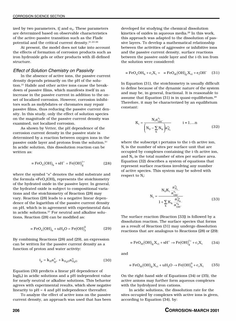
the model, corrosion rates were calculated for carbonsteel in aerated water in the presence of severalinhibitors. Figure 1 shows the dependence of thecalculated corrosion rate on the concentration ofthree inhibitors (monobasic phosphate, silicate, andchromate ions). In all cases, a fairly sharp transition

to passive behavior was observed as the concentra-tion of the inhibitor exceeded a certain thresholdvalue. This threshold value was very low for chro-mates and substantially higher for monobasic phos-phates and silicates. It is noteworthy that the modelrepresents the experimental corrosion rates with verygood accuracy.37

To examine how this behavior is reproduced bythe model, Figure 2 shows the calculated currentdensity vs potential relationships for three concen-trations of silicate ions (0, 0.0014, and 0.008 m).Figure 2 includes the partial cathodic and anodicprocesses that were taken into account for the analy-sis. The dominant cathodic process was the reduc-tion of oxygen. This process, denoted by “B” in thefigure, proceeded under mass-transfer control asshown by the vertical portion of the oxygen reductionline. The iron oxidation process exhibited an active-passive transition, which was strongly influencedby the presence of inhibitors. Without silicate ions(Figure 2[a]), the oxygen reduction line intersectedthe iron oxidation line in the range of active dissolu-tion of iron. Correspondingly, the corrosion potentialwas low and the corrosion rate was substantial. Witha substantial concentration of silicate ions (Figure2[c]), the passive current density and critical currentdensity were substantially reduced. Subsequently,the oxygen reduction line intersected the iron oxida-tion line within the passive range. The corrosion po-tential increased substantially and the corrosion ratewas reduced. For intermediate concentrations of sili-cate ions (Figure 2[b]), the shape of the predicted ironoxidation line was such that three mixed potentialswere possible. This resulted in multiple steadystates, and the system oscillated between corrosionin the active and passive states. This is reflected inFigure 1 by several vertical portions of the calculatedline, which correspond to the range of predicted cor-rosion rates for given conditions. Although this be-havior cannot be unequivocally corroborated, it isconsistent with experimental data in the intermedi-ate concentration range that corresponds to theactive-passive transition.

After verifying the predictions for inhibitors inpure aerated water, the model was applied to morecomplex systems. Figure 3 shows the dependence ofthe corrosion rate of carbon steel in simulated cool-ing water as a function of pH and the amount ofadded nitrate ions. Simulated cooling water containssmall, but not negligible, concentrations of chlorideand sulfate ions, which contribute to the breakdownof passive films. Thus, the chloride and sulfate ionscounteract the effect of the inhibitor ions. The com-peting effect of various ions is taken into account byEquation (39) for the passive current density. Asshown in Figure 3, the corrosion rate is stronglyaffected by pH. This was caused by the effect of pHon the passive current density (Equation [39]) and

(a)

(b)

(c)FIGURE 1. Effect of monobasic phosphate, silicate, and chromateions on the corrosion rate of carbon steel in aerated water at 25°C.The lines were calculated from the model, and the symbols denotethe data of Pryor and Cohen.38



the contribution of the proton reduction reaction(Equation [9]), which becomes significant at lowerpH values. As shown in Figure 3, the effect of pHand nitrite concentration is accurately reproducedby the model.

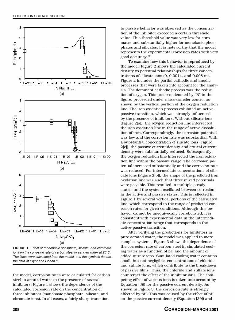
The electrochemical model is particularly suit-able for studying the effects of mixtures of inhibitors.This is shown in Figure 4 for the corrosion rate ofcarbon steel in simulated cooling water in the pres-ence of a mixed molybdate + nitrite inhibitor. Param-eters of the electrochemical model were adjustedbased on limited experimental data for systems witha single inhibitor.37-38 With such parameters, themodel can be used to make predictions for mixedsystems. As shown in Figure 4, the model correctlypredicted the pH dependence of corrosion rates inthe mixed-inhibitor system.

It is particularly interesting to apply the modelto study the synergism of inhibitors with dissolvedoxygen. Figure 5 shows results of calculations forcarbon steel in simulated cooling water inhibitedwith a mixture of sodium nitrite (NaNO2) and sodiummolybdate (Na2MoO4) with varying composition.The total amount of inhibitor (NaNO2 + Na2MoO4) is500 mg/L, and the amount of dissolved oxygen is1, 2.5, or 5 mg/L. The corrosion rate for the systeminhibited with only NaNO2 (i.e., for 0 mg MoO4) didnot depend on the concentration of oxygen. This wascaused by the fact that nitrate ions have oxidizingproperties (Equation [22]) and contribute to increas-ing the corrosion potential. However, molybdate ionsare not oxidizing and their effect is limited to reduc-ing the passive current density (Equation [39]). How-ever, the reduction of the passive current density wasnot sufficient, in this case, to achieve passive behav-ior. Therefore, the corrosion rate of the system inhib-

FIGURE 2. Predicted current density-potential relationships, includingpartial anodic and cathodic processes, for carbon steel in aeratedwater with: (a) no Na2SiO3, (b) 0.0014 m Na2SiO3, and (c) 0.008 mNa2SiO3. The partial processes are denoted by A through D, whereA: H2O = 0.5 H2 + OH– – e–, B: O2 + 4H+ = 2H2O – 4e–, C: Fe = Fe2+ +2e–, and D: 2H2O = O2 + 4H+ + 4e–.

FIGURE 3. Corrosion rates of carbon steel in simulated cooling water(7 × 10–3 m NaCl, 5.4 × 10–3 m Na2SO4, 6.25 × 10–4 CaCO3, and6.25 × 10–4 m MgCO3) as a function of pH and the concentration ofadded nitrite ions. The lines were obtained from the model, and thesymbols denote the data of Mustafa and Dulal.39

(a)

(b)

(c)



ited with only molybdate ions (i.e., for 500 mg MoO4)depends on the concentration of dissolved oxygen.Dissolved oxygen increased the corrosion potentialso that the passive range was reached. Thus, thecorrosion rate in the presence of molybdate ions wasreduced when the concentration of oxygen was suffi-ciently high. Figure 5 also illustrates the synergybetween molybdate and nitrite ions for the inhibition

of corrosion of carbon steel. Even with small concen-trations of dissolved oxygen, the combination ofnitrites and molybdates was sufficient to reduce thecorrosion rate. Experimental data for this systemshow substantial scattering.39 However, the predictedtrends are in agreement with the data.

CONCLUSIONS

❖ A mechanistic model was developed for simulatingthe rates of general corrosion of selected metals inaqueous solutions. The model consists of athermophysical module that provides comprehensivespeciation calculations and an electrochemical mod-ule that predicts the partial reduction and oxidationprocesses on the surface of the metal. The electro-chemical module is capable of reproducing theactive-passive transition and the effect of solutionspecies on passivity. The model was incorporatedinto a program that can be used to study theeffect of conditions such as temperature, pressure,pH, solution composition, or flow velocity on corro-sion rates.❖ Model predictions were verified for a number ofsystems that included corrosion inhibitors. Also,the model was validated in previous papers forCO2/H2S corrosion and systems containing concen-trated brines.12-13 In all cases, good agreement withexperimental data was obtained. Thus, the modelcan be used to predict corrosion rates in multicom-ponent systems for which experimental data arenot available.

REFERENCES

1. C. de Waard, D.E. Milliams, Corrosion 31 (1975): p. 177-181.2. C. de Waard, U. Lotz, D.E. Milliams, Corrosion 47 (1991): p.

976.3. S. Nesic, J. Postlethwaite, S. Olsen, Corrosion 52 (1996): p.

280-294.4. R. Zhang, M. Gopal, W.P. Jepson, “Development of a Mechanis-

tic Model for Predicting Corrosion Rate in Multiphase Oil/Water/Gas Flows,” CORROSION/97, paper no. 601 (Houston,TX: NACE International, 1997).

5. L.K. Gatzky, R.H. Hausler, “A Novel Correlation of TubingCorrosion Rates and Gas Production Rates,” in Advances inCO2 Corrosion, eds. R.H. Hausler, H.P. Godard, vol. 1 (Houston,TX: NACE, 1984), p. 87.

6. M.R. Bonis, J.L. Crolet, “Basics of the Prediction of the Risksfor CO2 Corrosion in Oil and Gas Wells,” CORROSION/89,paper no. 466 (Houston, TX: NACE, 1989).

7. J.D. Garber, F.H. Walters, R.R. Alapati, C.D. Adams, “DownholeParameters to Predict Tubing Life and Mist Flow in GasCondensate Wells,” CORROSION/94, paper no. 25 (Houston,TX: NACE, 1994).

8. S. Srinivasan, R.D. Kane, “Prediction of Corrosivity of CO2/H2SProduction Environments,” CORROSION/96, paper no. 11(Houston, TX: NACE, 1996).

9. A. Dugstad, L. Lunde, K. Videm, “Parametric Study of CO2

Corrosion of Carbon Steel,” CORROSION/94, paper no. 14(Houston, TX: NACE, 1994).

10. E. Dayalan, F.D. de Moraes, J.R. Shadley, S.A. Shirazi, E.F.Rybicki, “CO2 Corrosion Prediction in Pipe Flow Under FeCO3

Scale-Forming Conditions,” CORROSION/98, paper no. 51(Houston, TX: NACE, 1998).

11. D.D. Macdonald, M. Urquidi-Macdonald, Corrosion 46 (1990):p. 380-390.

FIGURE 4. Corrosion rates of carbon steel in simulated cooling water(7 × 10–3 m NaCl, 5.4 × 10–3 m Na2SO4, 6.25 × 10–4 CaCO3, and 6.25× 10–4 m MgCO3) as a function of pH in the presence of 400 ppm ofmolybdate ions and 400 ppm of nitrite ions. The lines were obtainedfrom the model, and symbols denote the data of Mustafa and Dulal.39

FIGURE 5. Corrosion rates in simulated cooling water (7 × 10–3 mNaCl, 5.4 × 10–3 m Na2SO4, 6.25 × 10–4 CaCO3, and 6.25 × 10–4 mMgCO3) at 60°C inhibited with a mixture of NaNO2 and N2MoO4 withvarying composition. The total amount of dissolved inhibitor is500 mg/L, and the amount of dissolved oxygen is 1, 2.5 ,or 5 mg/L.The lines were obtained from the model, and the symbols denotethe data of Weber, et al.40 Vertical portions of the lines denote therange between the highest and lowest rate predicted for a givencomposition.



12. A. Anderko, R.D. Young, “Simulation of CO2/H2S CorrosionUsing Thermodynamic and Electrochemical Models,” CORRO-SION/99, paper no. 31 (Houston, TX: NACE, 1999).

13. A. Anderko, R.D. Young, “Computer Modeling of Corrosion inAbsorption Cooling Cycles,” CORROSION/99, paper no. 243(Houston, TX: NACE, 1999).

14. J.F. Zemaitis, Jr., D.M. Clark, M. Rafal, N.C. Scrivner,Handbook of Aqueous Electrolyte Thermodynamics (New York,NY: AIChE, 1986), p. 852.

15. M. Rafal, J.W. Berthold, N.C. Scrivner, S.L. Grise, “Models forElectrolyte Solutions,” in Models for Thermodynamic and PhaseEquilibria Calculations, ed. S.I. Sandler (New York, NY: M.Dekker, 1995), p. 601-670.

16. D.M. Drazic, “Iron and Its Electrochemistry in an Active State,”in Modern Aspects of Electrochemistry, eds. B.E. Conway,J.O’M. Bockris, R.E. White, no. 19 (New York, NY: PlenumPress, 1989), p. 69-192.

17. J.O’M. Bockris, D. Drazic, A.R. Despic, Electrochim. Acta 4(1961): p. 325-361.

18. N.G. Smart, J.O’M. Bockris, Corrosion 48 (1992): p. 277-280.19. J.M. West, Electrodeposition and Corrosion Processes (New

York, NY: Van Nostrand, 1964), p. 36.20. M. Keddam, “Anodic Dissolution,” in Corrosion Mechanisms in

Theory and Practice, eds. P. Marcus, J. Oudar (New York, NY:M. Dekker, 1995), p. 55-122.

21. K.J. Vetter, Electrochemical Kinetics (New York, NY: AcademicPress, 1967), pp. 516, 755.

22. U. Ebersbach, K. Schwabe, K. Ritter, Electrochim. Acta 12(1967): p. 927-938.

23. N. Sato, T. Noda, K. Kudo, Electrochim. Acta 19 (1974): p.471-475.

24. P. Lorbeer, W.J. Lorenz, Corros. Sci. 21 (1981): p. 79.25. P. Lorbeer, K. Juttner, W.J. Lorenz, Werkst. Korros. 34 (1983):

p. 290.26. K.E. Heusler, K.G. Weil, K.F. Bonhoeffer, Z. Physik. Chem. Neue

Folge 15 (1958): p. 149.27. K.J. Vetter, Z. Elektrochem. 59 (1955): p. 67.28. M.A. Blesa, P.J. Morando, A.E. Regazzoni, Chemical Dissolution

of Metal Oxides (Boca Raton, FL: CRC Press, 1994), p. 172.29. K.J. Vetter, F. Gorn, Electrochim. Acta 18 (1973): p. 321.30. K.E. Heusler, Corros. Sci. 29 (1989): p. 131.31. J.O’M. Bockris, M.A. Genshaw, V. Brusic, H. Wroblowa,

Electrochim. Acta 16 (1971): p. 1,859.32. K.E. Heusler, B. Kusian, D. McPhail, Ber. Bunsenges. Phys.

Chem. 94 (1990): p. 1,443.33. B.D. Craig, D.S. Anderson, eds., Handbook of Corrosion Data

(Materials Park, OH: ASM International, 1995), p. 1-998.34. P.B. Mathur, T. Vasudevan, Corrosion 38 (1982): p. 171-178.35. M.A. Stranick, Corrosion 40 (1984): p. 296-302.36. E.A. Lizlovs, Corrosion 32 (1976): p. 263.37. M.J. Pryor, M. Cohen, J. Electrochem. Soc. 100 (1953): p.

203-215.38. C.M. Mustafa, S.M. Shahinoor Islam Dulal, Corrosion 52

(1996): p. 16.39. T.R. Weber, M.A. Stranick, M.S. Vukasovich, Corrosion 42

(1986): p. 542.40. H.C. Helgeson, D.H. Kirkham, G.C. Flowers, Amer. J. Sci. 281

(1981): p. 1,249-1,516.41. J.C. Tanger, H.C. Helgeson, Amer. J. Sci. 288 (1988): p. 19-98.42. E.L. Shock, H.C. Helgeson, Geochim. Cosmochim. Acta 52

(1988): p. 2,009-2,036.43. E.L. Shock, H.C. Helgeson, Geochim. Cosmochim. Acta 54

(1990): p. 915-943.44. D.A. Sverjensky, Rev. Mineral. 17 (1987): p. 177-209.45. L.A. Bromley, AIChE J. 19 (1973): p. 313-320.46. K.S. Pitzer, J. Phys. Chem. 77 (1973): p. 268-277.47. G. Soave, Chem. Eng. Sci. 27 (1972): p. 1,197-1,203.48. H.P. Meissner, “Thermodynamics of Aqueous Systems with

Industrial Applications,” S.A. Newman, ed., American ChemicalSociety (ACS) Symp. Ser. 133 (Washington, DC: ACS, 1980),p. 495-511.

49. V.G. Levich, Physicochemical Hydrodynamics (Englewood Cliffs,NJ: Prentice-Hall, 1962), p. 700.

50. A. Anderko, M.M. Lencka, Ind. Eng. Chem. Res. 37 (1998): p.2,878-2,888.

51. M.M. Lencka, A. Anderko, S.J. Sanders, R.D. Young, Int. J.Thermophysics 19 (1998): p. 367-378.

52. F.P. Berger, K.-F.F.L. Hau, Int. J. Heat Mass Trans. 20 (1977):p. 1,185-1,194.

53. M. Eisenberg, C.W. Tobias, C.R. Wilke, J. Electrochem. Soc.101 (1954): p. 306-319.

APPENDIX A—THERMODYNAMIC FRAMEWORK

In a multicomponent system, the partial molalGibbs energy of the i-th species is related to themolality (mi) by:

G G RT mi io

i i= + ln γ (A-1)

where G—

i0 is the standard-state partial Gibbs energy

and �i is the activity coefficient. Thus, the thermo-dynamic properties of the system can be calculatedif the standard-state Gibbs energies are availablefor all species as functions of temperature and pres-sure (i.e., G

—i0 [T,P]), and the activity coefficients are

known as functions of the composition vector (m)and temperature (i.e., �i[m,T]). From basic thermo-dynamics, the standard-state Gibbs energy offormation G

—i0 (T,P) can be calculated as a function

of temperature and pressure if the following dataare available:

—Gibbs energy of formation at a referencetemperature and pressure (usually, Tr = 298.15 Kand Pr = 1 bar);

—Enthalpy of formation at Tr and Pr;—Entropy at Tr and Pr;—Heat capacity as a function of temperature

and pressure; and—Volume as a function of temperature and

pressure.The key to representing the standard-state prop-

erties over substantial temperature and pressureranges is the accurate knowledge of the heat capacityand volume. For this purpose, the Helgeson-Kirkham-Flowers-Tanger (HKFT) equation of state isused.40-41 This equation accurately represents thestandard-state thermodynamic functions for aque-ous, ionic, or neutral species as functions of tem-perature and pressure. In its revised form,42 theHKFT equation is capable of reproducing the stan-dard-state properties up to 1,000°C and 5 kbar.

The HKFT equation is based on the solvationtheory and expresses the standard-state thermody-namic functions as sums of structural and solvationcontributions, the latter being dependent on theproperties of the solvent (i.e., water). The standardpartial molal volume (V

—0) and heat capacity (C—

p0) are

given by:

V aa

Pa

aP

TQ

P T

0 12

34

1 11

= ++

+ ++

−

− + −

∂∂

Ψ Ψ

Θω

εω (A-2)



C cc

T

T

T

a P P aPP

TX

TYT

TT

p

rr

p p

01

22 3

3 4

2

2

2

21

1

= +−( )

−−( )

−( ) + ++

+

+ ∂∂

− −

∂∂

Θ Θ

ΨΨ

ln ω

ωε

ω

(A-3)

where a1, a2, a3, a4, c1, and c2 represent species-dependent nonsolvation parameters; Tr is the refer-ence temperature of 298.15 K; Pr is the referencepressure of 1 bar; Ψ and Θ refer to solvent param-eters equal to 2,600 bars and 228 K, respectively;and Q, X, and Y denote the Born functions given by:

QP T

= ∂∂

1ε

εln (A-4)

XT T

P p

= ∂∂

− ∂∂

1 2

2

2

εε εln ln

(A-5)

YT p

= ∂∂

1ε

εln (A-6)

where ε is the dielectric constant of water and ωstands for the Born coefficient, which is defined forthe j-th aqueous species by:

ω ω ωj jabs

j HabsZ≡ − + (A-7)

In Equation (A-7), Zj is the charge on the j-th aque-ous species, ωH+

abs refers to the absolute Born coeffi-cient of the hydrogen ion, and ω j

abs designates theabsolute Born coefficient of the j-th species given by:

ω jabs j

e j

N e Z

r

0 2 2

2 , (A-8)

where N0 is the Avogadro number, e is the electroncharge, and re,j denotes the effective electrostaticradius of the j-th species, which is related to thecrystallographic radius rx,j by:

r r z k ge j x j j z, ,= + +( ) (A-9)

where kz represents a charge-dependent constantequal to 0.0 for anions and 0.94 for cations, andg denotes a generalized function of temperature anddensity. Thus, the HKFT equation expresses the heatcapacity and volume as functions of pure water prop-erties and seven empirical parameters, which havebeen tabulated for large numbers of ions, complexes,

and neutral inorganic and organic molecules. Theremaining thermodynamic properties are obtained bythermodynamic integration using the values of theGibbs energy, enthalpy, and entropy at referencetemperature and pressure as integration constants.

If the HKFT equation parameters are not avail-able from the regression of experimental data, theycan be estimated. For this purpose, Shock andHelgeson presented correlations for most solutionspecies except complexes.42-43 Sverjensky developedan estimation method for several classes of com-plexes.44 In addition to the HKFT equation param-eters, these methods make it possible to predict thereference-state enthalpy and entropy if the reference-state Gibbs energy is known. These and other esti-mation techniques have been reviewed in detail byRafal, et al.15

The activity coefficient model used for represent-ing the solution nonideality is an extended form of anexpression developed by Bromley.45 The Bromleyequation is a combination of the Debye-Hückel termfor long-range electrostatic interactions and a semi-empirical expression for short-range interactionsbetween cations and anions. In a multicomponentsystem, the activity coefficient of an ion i is given by:

log

. .

.

/

/γ ii i j

j

NO

ij i j

i j

ij ij ij j

Az II

z z

B z z

z zI

B C I D I m

= −+

++

+( )+

+ + +

∑2 1 2

1 2

2

22

1 2

0 06 0 6

11 5

(A-10)

where A is the Debye-Hückel coefficient that dependson temperature and solvent properties, zi is the num-ber of charges on ion i, I is the ionic strength (i.e.,I = 0.5 Σ zi

2mi), NO is the number of ions with chargesopposite to that of ion i, and Bij, Cij, and Dij are em-pirical, temperature-dependent cation-anion interac-tion parameters. Bromley’s original formulationcontains only one interaction parameter, Bij, which issufficient for systems with moderate ionic strength.45

For concentrated systems, the two additional coeffi-cients Cij and Dij usually become necessary. Thethree-parameter form of the Bromley model is ca-pable of reproducing activity coefficients in solutionswith ionic strength up to 30 mol/kg. The tempera-ture dependence of the Bij, Cij, and Dij parameters isusually expressed using a simple quadratic function.

The Bromley model is restricted to interactionsbetween cations and anions. For ion-molecule andmolecule-molecule interactions, the well-knownPitzer model is used.46 To calculate the fugacities ofcomponents in the gas phase, the Redlich-Kwong-



Soave equation of state is used.47 In the absence ofsufficient experimental data, reasonable predictionscan be made using a method proposed by Meissner,48

which makes it possible to extrapolate the activitycoefficients to higher ionic strengths based on onlya single, experimental, or predicted data point.

APPENDIX B—CALCULATIONOF THE MASS-TRANSFER COEFFICIENT

The mass-transfer coefficient km (Equations [13]and [20]) can be calculated once the flow geometry isassumed. For example, for a rotating disk, the equa-tion of Levich holds:49

k Dm = −0 62 2 3 1 6 1 2. / / /ν ω (B-1)

where D is the diffusion coefficient of the species thatundergoes the electrode reaction, � is the kinematicviscosity, and ω is the rotation velocity. The diffusioncoefficient and viscosity are calculated as functionsof temperature and concentration using the methodsdeveloped by Anderko and Lencka50 and Lencka,et al.,51 respectively.

For straight pipe and rotating cylinder geometry,the mass-transfer coefficient can be expressed interms of the dimensionless Reynolds (Re) andSchmidt (Sc) numbers. These numbers are definedby:

Re = ννd

(B-2)

ScD

= ν (B-3)

where ν is the linear velocity and d is the diameter.For single-phase flow in a straight pipe, the correla-tion of Berger and Hau can be used:52

k dD

Scm = 0 0165 0 86 0 33. Re . . (B-4)

For a rotating cylinder, the correlation of Eisenberg,et al., applies:53

k dD

Scm = 0 0791 0 70 0 356. Re . . (B-5)

computation of rates of general corrosion using ...computation of rates of general corrosion using...

Documents